<pubnumber>842B94003</pubnumber>
<title>CWA Section 403: Procedural and Monitoring Guidance</title>
<pages>352</pages>
<pubyear>1994</pubyear>
<provider>NEPIS</provider>
<access>online</access>
<operator>BO</operator>
<scandate>04/15/97</scandate>
<origin>hardcopy</origin>
<type>single page tiff</type>
<keyword>monitoring marine methods discharge water environmental usepa sampling species section fish sediment biological data sample samples analysis quality considerations benthic</keyword>
<author> Tetra Tech, Inc., Arlington, VA.;Environmental Protection Agency, Washington, DC. Office of Wetlands, Oceans and Watersheds. United States. Environmental Protection Agency. Office of Water. Office of Wetlands, Oceans and Watersheds. ; Tetra Tech, Inc.</author>
<publisher>U.S. Environmental Protection Agency, Office of Water ,</publisher>
<subject>Water pollution monitoring; Ocean waste disposal; Aquatic ecology; Permits; Water pollution control; Marine biology; Biological accumulation; Environmental impacts; Environmental protection; Estuaries; Benthos; Water chemistry; Clean Water Act; Water pollution standards; Pollution regulations; Discharge(Water); Section 403; NPDES(National Pollutant Discharge Elimination System) Marine pollution--Sampling--Handbooks, manuals, etc ; Water--Pollution--Handbooks, manuals, etc</subject>
<abstract>The purpose of the document is to provide the Regions and NPDES-authorized States with a framework for the decision-making process to be followed in making a section 403 determination and to provide them with guidance for identifying the type and level of monitoring that should be required as part of a permit issued under the no irreparable harm provisions of section 403. Chapter 2 of the document presents an explanation of, and procedural guidance for, the overall process to be followed when issuing an NPDES permit in compliance with section 403 of the Clean Water Act. Chapter 3 discusses options for monitoring under the basis of no irreparable harm. Chapter 4 presents a summary of monitoring methods with potential applications to 403 discharges. </abstract>
United States
Environmental Protection
Agency
Office of Water
(4504F)
EPA 842-B-94-003
March 1994
CWA Section 403:
Procedural and Monitoring
Guidance
Recycled/Recyclable
Printed with Soy/Canola Ink on paper that
contains at least 50% post-consumer recycled fiber
image:
 image:
 CWA SECTION 403: PROCEDURAL AND
MONITORING GUIDANCE
March 1994
United States Environmental Protection Agency
Office of Wetlands, Oceans and Watersheds
Oceans and Coastal Protection Division
Washington, DC
image:
CWA SECTION 403: PROCEDURAL AND
MONITORING GUIDANCE
March 1994
United States Environmental Protection Agency
Office of Wetlands, Oceans and Watersheds
Oceans and Coastal Protection Division
Washington, DC
image:
 DISCLAIMER
This document has been reviewed in accordance with U.S. Environmental Protection
Agency policy and approved for publication. Mention of trade names or commercial
products does not constitute endorsement or recommendation for use.
image:
DISCLAIMER
This document has been reviewed in accordance with U.S. Environmental Protection
Agency policy and approved for publication. Mention of trade names or commercial
products does not constitute endorsement or recommendation for use.
image:
 CONTENTS
Page
TABLES .... ;. .v: ....... ix
FIGURES. xi
ACKNOWLEDGMENTS xiii
ABBREVIATIONS xv
GLOSSARY xvii
EXECUTIVE SUMMARY xxv
1. INTRODUCTION 1
1.1 THE OCEAN DISCHARGE CRITERIA 2
1.2 PURPOSE OF: THIS DOCUMENT 3
1.3 DOCUMENT FORMAT 3
2. SECTION 403 PROCEDURE 5
2.1 BACKGROUND 5
2.1.1 The Role of the Ocean Discharge Criteria
in NPDES Permit Issuance 5
2.1.2 Applicability of Section 403 5
2.1.3 Individual or General Permit 7
2.2 GENERAL PROCEDURE 8
2.2.1 Request for Issuance/Reissuance of a
Section 402 Permit 8
2.2.2 Determination of Information Requirements 10
2.2.3 Determination of No Unreasonable Degradation 11
2.2.4 Decision to Issue/Reissue or Deny a Permit 14
.2.2.5 Insufficient Information 14
image:
CONTENTS
Page
TABLES .... ;. .v: ....... ix
FIGURES. xi
ACKNOWLEDGMENTS xiii
ABBREVIATIONS xv
GLOSSARY xvii
EXECUTIVE SUMMARY xxv
1. INTRODUCTION 1
1.1 THE OCEAN DISCHARGE CRITERIA 2
1.2 PURPOSE OF: THIS DOCUMENT 3
1.3 DOCUMENT FORMAT 3
2. SECTION 403 PROCEDURE 5
2.1 BACKGROUND 5
2.1.1 The Role of the Ocean Discharge Criteria
in NPDES Permit Issuance 5
2.1.2 Applicability of Section 403 5
2.1.3 Individual or General Permit 7
2.2 GENERAL PROCEDURE 8
2.2.1 Request for Issuance/Reissuance of a
Section 402 Permit 8
2.2.2 Determination of Information Requirements 10
2.2.3 Determination of No Unreasonable Degradation 11
2.2.4 Decision to Issue/Reissue or Deny a Permit 14
.2.2.5 Insufficient Information 14
image:
 CONTENTS (continued)
OPTIONS FOR MONITORING UNDER THE BASIS OF "NO
IRREPARABLE HARM"
17
3.1 BACKGROUND 17
3.2 CRITERIA FOR EVALUATING THE POTENTIAL
FOR ENVIRONMENTAL IMPACT 18
3.2.1 Major/Minor Discharges ... 18
3.2.2 Discharges to Stressed Waters 20
3.2.3 Discharges to Sensitive Biological Areas 21
3.2.4 Presence of Other Discharges in the Area 25
3.3 MONITORING REQUIREMENTS BASED ON PERCEIVED
POTENTIAL ENVIRONMENTAL THREAT 25
3.3.1 Minimal Potential Threat 25
3.3.2 Moderate Potential Threat 27
3.3.3 High Potential Threat 29
3.4 SUMMARY 30
4. SUMMARY OF MONITORING METHODS 31
4.1 PHYSICAL CHARACTERISTICS 40
4.1.1 Rationale 40
4.1.2 Monitoring Design Considerations 40
4.1.3 Analytical Methods Considerations 42
4.1.4 QA/QC Considerations 48
4.1.5 Statistical Design Considerations 51
4.1.6 Use of Data 52
4.1.7 Summary and Recommendations 52
4.2 WATER CHEMISTRY 56
4.2.1 Rationale 56
4.2.2 Monitoring Design Considerations 56
4.2.3 Analytical Methods Considerations 58
4.2.4 QA/QC Considerations 63
4.2.5 Statistical Design Considerations 66
4.2.6 Use of Data 67
4.2.7 Summary and Recommendations 68
Iv
image:
CONTENTS (continued)
OPTIONS FOR MONITORING UNDER THE BASIS OF "NO
IRREPARABLE HARM"
17
3.1 BACKGROUND 17
3.2 CRITERIA FOR EVALUATING THE POTENTIAL
FOR ENVIRONMENTAL IMPACT 18
3.2.1 Major/Minor Discharges ... 18
3.2.2 Discharges to Stressed Waters 20
3.2.3 Discharges to Sensitive Biological Areas 21
3.2.4 Presence of Other Discharges in the Area 25
3.3 MONITORING REQUIREMENTS BASED ON PERCEIVED
POTENTIAL ENVIRONMENTAL THREAT 25
3.3.1 Minimal Potential Threat 25
3.3.2 Moderate Potential Threat 27
3.3.3 High Potential Threat 29
3.4 SUMMARY 30
4. SUMMARY OF MONITORING METHODS 31
4.1 PHYSICAL CHARACTERISTICS 40
4.1.1 Rationale 40
4.1.2 Monitoring Design Considerations 40
4.1.3 Analytical Methods Considerations 42
4.1.4 QA/QC Considerations 48
4.1.5 Statistical Design Considerations 51
4.1.6 Use of Data 52
4.1.7 Summary and Recommendations 52
4.2 WATER CHEMISTRY 56
4.2.1 Rationale 56
4.2.2 Monitoring Design Considerations 56
4.2.3 Analytical Methods Considerations 58
4.2.4 QA/QC Considerations 63
4.2.5 Statistical Design Considerations 66
4.2.6 Use of Data 67
4.2.7 Summary and Recommendations 68
Iv
image:
 Section 403 Procedural and Monitoring Guidance
CONTENTS (continued)
4.3 SEDIMENT CHEMISTRY 71
4.3.1 Rationale 71
4.3.2 Monitoring Design Considerations 71
4.3.3 Analytical Methods Considerations 79
4.3.4 QA/QC Considerations 83
4.3.5 Statistical Design Considerations 88
4.3.6 Use of Data 89
4.3.7 Summary and Recommendations 90
4.4 SEDIMENT GRAIN SIZE 93
4.4.1 Rationale 93
4.4.2 Monitoring Design Considerations 93
4.4.3 Analytical Methods Considerations 98
4.4.4 QA/QC Considerations 100
4.4.5 Statistical Design Considerations 101
4.4.6 Use of Data 102
4.4.7 Summary and Recommendations 102
4.5 BENTHIC COMMUNITY STRUCTURE 105
4.5.1 Rationale 105
4.5.2 Monitoring Design Considerations 106
4.5.3 Analytical Methods Considerations 114
4.5.4 QA/QC Considerations 121
4.5.5 Statistical Design Considerations 123
4.5.6 Use of Data 124
4.5.7 Summary and Recommendations 124
4.6 FISH AND SHELLFISH PATHOBIOLOGY 127
4.6.1 Rationale 127
4.6.2 Monitoring Design Considerations 129
4.6.3 Analytical Methods Considerations 130
4.6.4 QA/QC Considerations 135
4.6.5 Statistical Design Considerations 135
4.6.6 Use of Data 136
4.6.7 Summary and Recommendations 139
4.7 FISH POPULATIONS 143
4.7.1 Rationale 143
4.7.2 Monitoring Design Considerations 144
4.7.3 Analytical Methods Considerations 146
4.7.4 QA/QC Considerations 150
image:
Section 403 Procedural and Monitoring Guidance
CONTENTS (continued)
4.3 SEDIMENT CHEMISTRY 71
4.3.1 Rationale 71
4.3.2 Monitoring Design Considerations 71
4.3.3 Analytical Methods Considerations 79
4.3.4 QA/QC Considerations 83
4.3.5 Statistical Design Considerations 88
4.3.6 Use of Data 89
4.3.7 Summary and Recommendations 90
4.4 SEDIMENT GRAIN SIZE 93
4.4.1 Rationale 93
4.4.2 Monitoring Design Considerations 93
4.4.3 Analytical Methods Considerations 98
4.4.4 QA/QC Considerations 100
4.4.5 Statistical Design Considerations 101
4.4.6 Use of Data 102
4.4.7 Summary and Recommendations 102
4.5 BENTHIC COMMUNITY STRUCTURE 105
4.5.1 Rationale 105
4.5.2 Monitoring Design Considerations 106
4.5.3 Analytical Methods Considerations 114
4.5.4 QA/QC Considerations 121
4.5.5 Statistical Design Considerations 123
4.5.6 Use of Data 124
4.5.7 Summary and Recommendations 124
4.6 FISH AND SHELLFISH PATHOBIOLOGY 127
4.6.1 Rationale 127
4.6.2 Monitoring Design Considerations 129
4.6.3 Analytical Methods Considerations 130
4.6.4 QA/QC Considerations 135
4.6.5 Statistical Design Considerations 135
4.6.6 Use of Data 136
4.6.7 Summary and Recommendations 139
4.7 FISH POPULATIONS 143
4.7.1 Rationale 143
4.7.2 Monitoring Design Considerations 144
4.7.3 Analytical Methods Considerations 146
4.7.4 QA/QC Considerations 150
image:
 CONTENTS (continued)
4.7.5 Statistical Design Considerations 150
4.7.6 Use of Data 151
4.7.7 Summary and Recommendations 152
4.8 PLANKTON: BIOMASS, PRODUCTIVITY, AND COMMUNITY
STRUCTURE/FUNCTION 154
4.8.1 Rationale 154
4.8.2 Monitoring Design Considerations 155
4.8.3 Analytical Methods Considerations 157
4.8.4 QA/QC Considerations 160
4.8.5 Statistical Design Considerations 161
4.8.6 Use of Data 161
4.8.7 Summary and Recommendations 162
4.9 HABITAT IDENTIFICATION METHODS 165
4.9.1 Rationale 165
4.9.2 Monitoring Design Considerations 166
4.9.3 Analytical Methods Considerations 167
4.9.4 QA/QC Considerations 171
4.9.5 Statistical Design Considerations 171
4.9.6 Use of Data 172
4.9.7 Summary and Recommendations 172
4.10 BIOACCUMULATION 175
4.10.1 Rationale 175
4.10.2 Monitoring Design Considerations 176
4.10.3 Analytical Methods Considerations 184
4.10.4 QA/QC Considerations 187
4.10.5 Statistical Design Considerations 188
4.10.6 Use of Data 189
4.10.7 Summary and Recommendations 189
4.11 PATHOGENS 192
4.11.1 Rationale 192
4.11.2 Monitoring Design Considerations 193
4.11.3 Analytical Methods Considerations 194
4.11.4 QA/QC Considerations 200
4.11.5 Statistical Design Considerations 201
4.11.6 Use of Data 201
4.11.7 Summary and Recommendations 201
vi
image:
CONTENTS (continued)
4.7.5 Statistical Design Considerations 150
4.7.6 Use of Data 151
4.7.7 Summary and Recommendations 152
4.8 PLANKTON: BIOMASS, PRODUCTIVITY, AND COMMUNITY
STRUCTURE/FUNCTION 154
4.8.1 Rationale 154
4.8.2 Monitoring Design Considerations 155
4.8.3 Analytical Methods Considerations 157
4.8.4 QA/QC Considerations 160
4.8.5 Statistical Design Considerations 161
4.8.6 Use of Data 161
4.8.7 Summary and Recommendations 162
4.9 HABITAT IDENTIFICATION METHODS 165
4.9.1 Rationale 165
4.9.2 Monitoring Design Considerations 166
4.9.3 Analytical Methods Considerations 167
4.9.4 QA/QC Considerations 171
4.9.5 Statistical Design Considerations 171
4.9.6 Use of Data 172
4.9.7 Summary and Recommendations 172
4.10 BIOACCUMULATION 175
4.10.1 Rationale 175
4.10.2 Monitoring Design Considerations 176
4.10.3 Analytical Methods Considerations 184
4.10.4 QA/QC Considerations 187
4.10.5 Statistical Design Considerations 188
4.10.6 Use of Data 189
4.10.7 Summary and Recommendations 189
4.11 PATHOGENS 192
4.11.1 Rationale 192
4.11.2 Monitoring Design Considerations 193
4.11.3 Analytical Methods Considerations 194
4.11.4 QA/QC Considerations 200
4.11.5 Statistical Design Considerations 201
4.11.6 Use of Data 201
4.11.7 Summary and Recommendations 201
vi
image:
 Section 403 Procedural and Monitoring Guidance
CONTENTS (continued)
4.12 EFFLUENT CHARACTERIZATION 204
4.12.1 Rationale 204
4.12.2 Monitoring Design Considerations ;. 206
4.12.3 Analytical Methods Considerations 206
4.12.4 QA/QC Considerations 208
4.12.5 Statistical Design Considerations 209
4.12.6 Use of Data 209
4.12.7 Summary and Recommendations 210
4.13 MESOCOSMS AND MICROCOSMS : 212
4.13.1 Rationale 212
4.13.2 Monitoring Design Considerations 213
4.13.3 Analytical Methods Considerations 213
4.13.4 QA/QC Considerations 214
4.13.5 Statistical Design Considerations 215
4.13.6 Use of Data 215
4.13.7 Summary and Recommendations 216
5.
LITERATURE CITED 219
APPENDIX A: MONITORING METHODS REFERENCES A-1
APPENDIX B: OCEAN DISCHARGE CRITERIA B-1
vii
image:
Section 403 Procedural and Monitoring Guidance
CONTENTS (continued)
4.12 EFFLUENT CHARACTERIZATION 204
4.12.1 Rationale 204
4.12.2 Monitoring Design Considerations ;. 206
4.12.3 Analytical Methods Considerations 206
4.12.4 QA/QC Considerations 208
4.12.5 Statistical Design Considerations 209
4.12.6 Use of Data 209
4.12.7 Summary and Recommendations 210
4.13 MESOCOSMS AND MICROCOSMS : 212
4.13.1 Rationale 212
4.13.2 Monitoring Design Considerations 213
4.13.3 Analytical Methods Considerations 213
4.13.4 QA/QC Considerations 214
4.13.5 Statistical Design Considerations 215
4.13.6 Use of Data 215
4.13.7 Summary and Recommendations 216
5.
LITERATURE CITED 219
APPENDIX A: MONITORING METHODS REFERENCES A-1
APPENDIX B: OCEAN DISCHARGE CRITERIA B-1
vii
image:
 image:
 TABLES
Table
Page
2-1. Ocean Discharge Guidelines 6
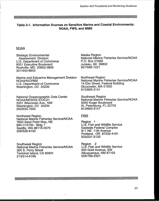
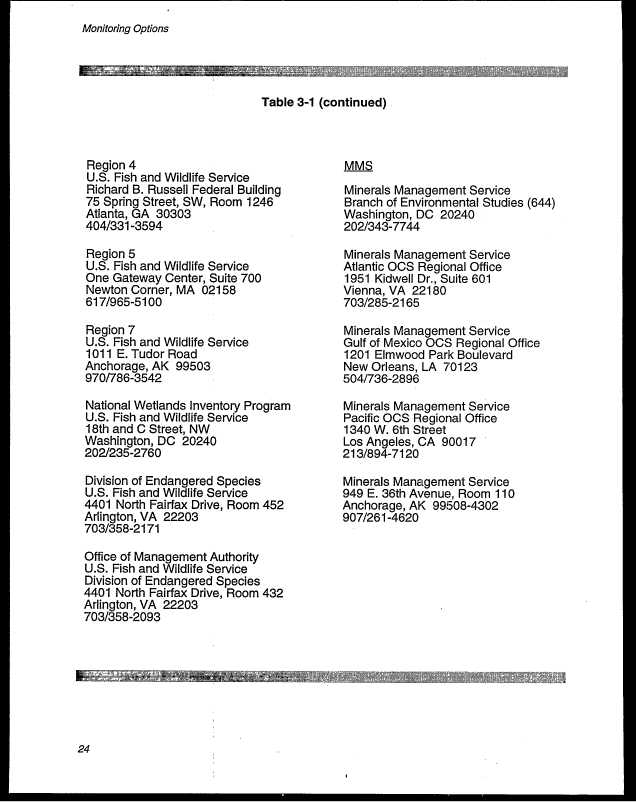
3-1. Information Sources on Sensitive Marine and Coastal Environments:
NOAA, FWS, and MMS 23
3-2. Characterization of Section 403 Discharges Based on the Potential for
Causing Environmental Impacts 26
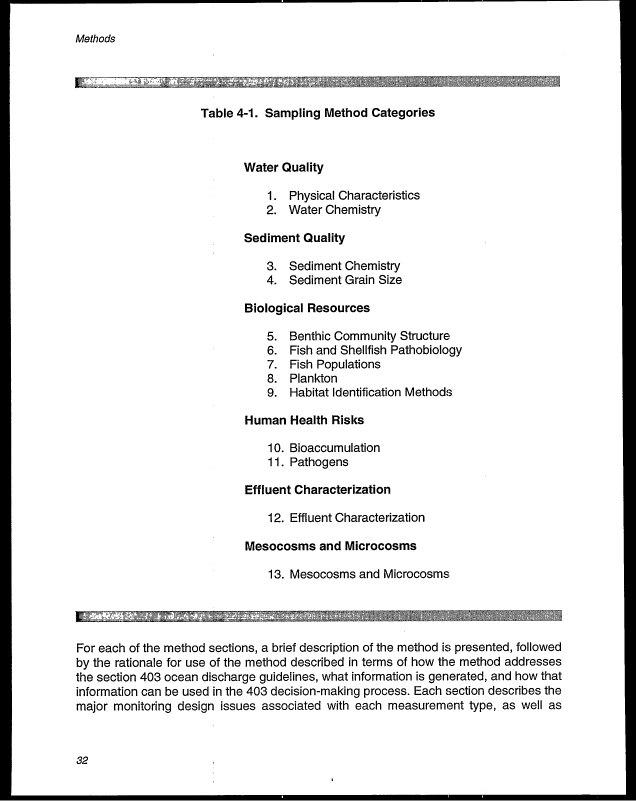
4-1. Sampling Method Categories 32
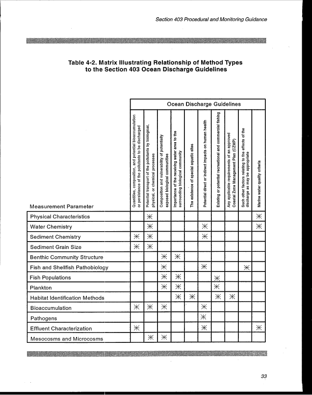
4-2. Matrix Illustrating Relationship of Method Types to the
Section 403 Ocean Discharge Guidelines 33
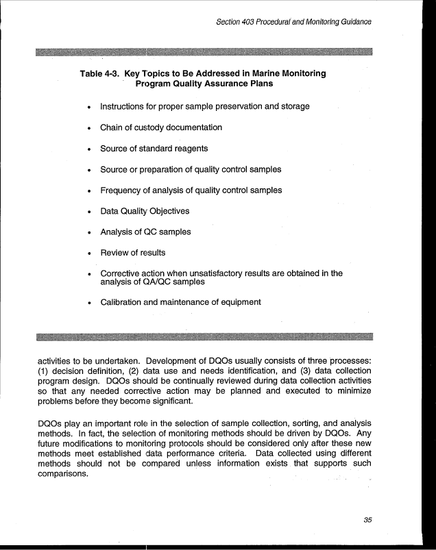
4-3. Key Topics to Be Addressed in Marine Monitoring
Quality Assurance Plans 35
4-4. QC Sample Types 36
4-5. List of Methods and Equipment 43
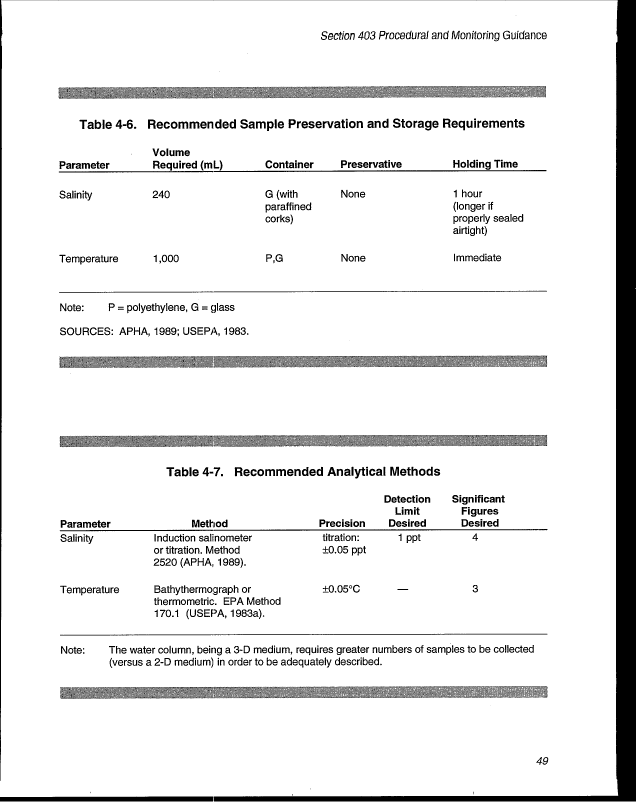
4-6. Recommended Sample Preservation and Storage Requirements 49
4-7. Recommended Analytical Methods 49
4-8. List of Analytical Techniques 60
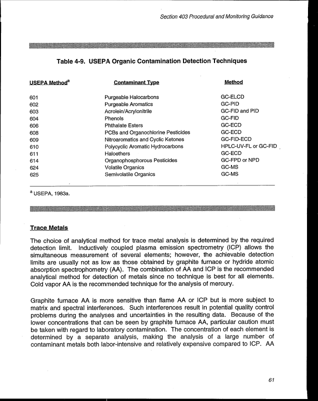
4-9. USEPA Organic Contamination Detection Techniques 61
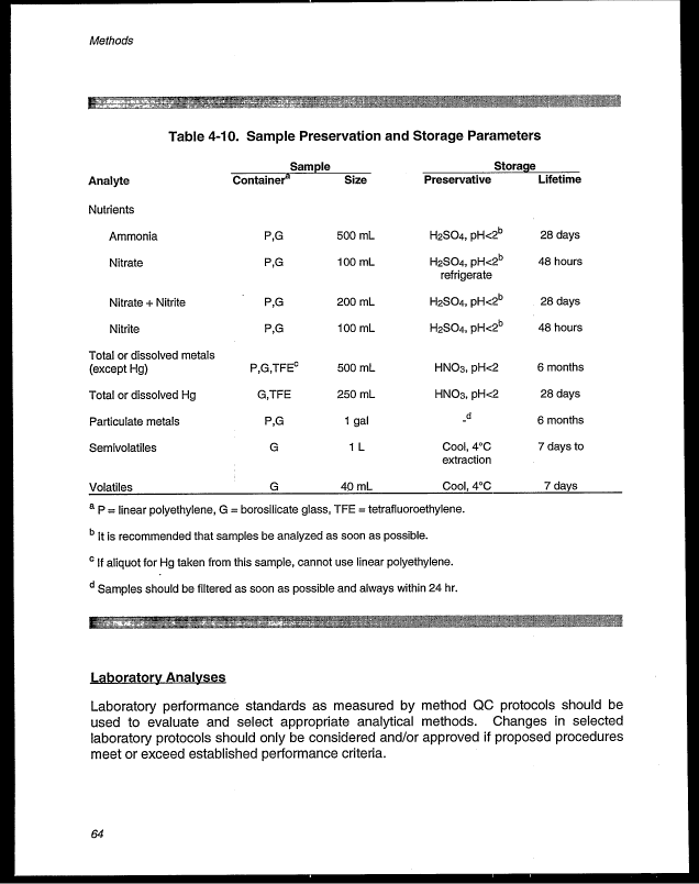
4-10. Sample Preservation and Storage Parameters 64
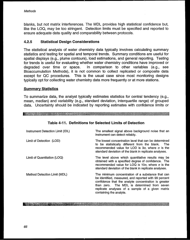
4-11. Definitions for Selected Limits of Detection 66
4-12. Sampling Containers, Preservation Requirements, and Holding
Times for Sediment Samples 73
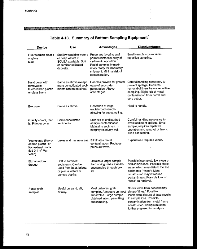
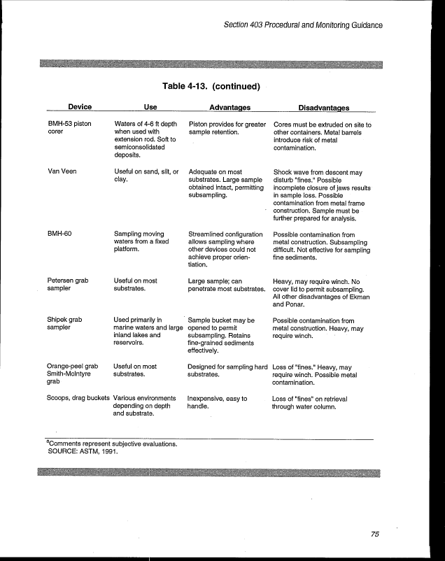
4-13. Summary of Bottom Sampling Equipment 74
IX
image:
TABLES
Table
Page
2-1. Ocean Discharge Guidelines 6
3-1. Information Sources on Sensitive Marine and Coastal Environments:
NOAA, FWS, and MMS 23
3-2. Characterization of Section 403 Discharges Based on the Potential for
Causing Environmental Impacts 26
4-1. Sampling Method Categories 32
4-2. Matrix Illustrating Relationship of Method Types to the
Section 403 Ocean Discharge Guidelines 33
4-3. Key Topics to Be Addressed in Marine Monitoring
Quality Assurance Plans 35
4-4. QC Sample Types 36
4-5. List of Methods and Equipment 43
4-6. Recommended Sample Preservation and Storage Requirements 49
4-7. Recommended Analytical Methods 49
4-8. List of Analytical Techniques 60
4-9. USEPA Organic Contamination Detection Techniques 61
4-10. Sample Preservation and Storage Parameters 64
4-11. Definitions for Selected Limits of Detection 66
4-12. Sampling Containers, Preservation Requirements, and Holding
Times for Sediment Samples 73
4-13. Summary of Bottom Sampling Equipment 74
IX
image:
 TABLES (continued)
Table page
4-14. List of Analytical Techniques 80
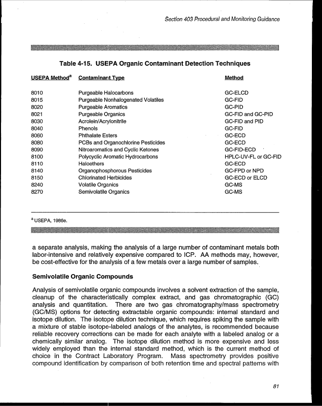
4-15. USEPA Organic Contaminant Detection Techniques 81
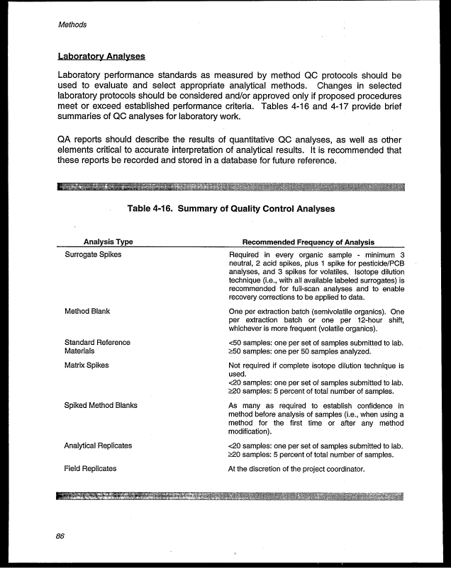
4-16. Summary of Quality Control Analyses 86
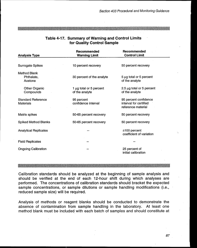
4-17. Summary of Warning and Control Limits for Quality Control Sample 87
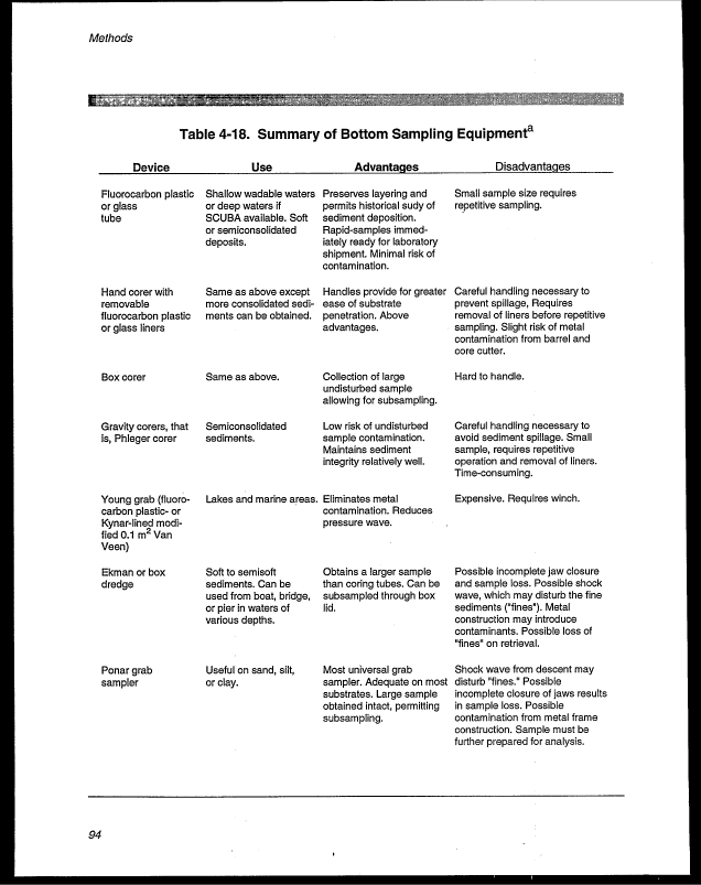
4-18. Summary of Bottom Sampling Equipment 94
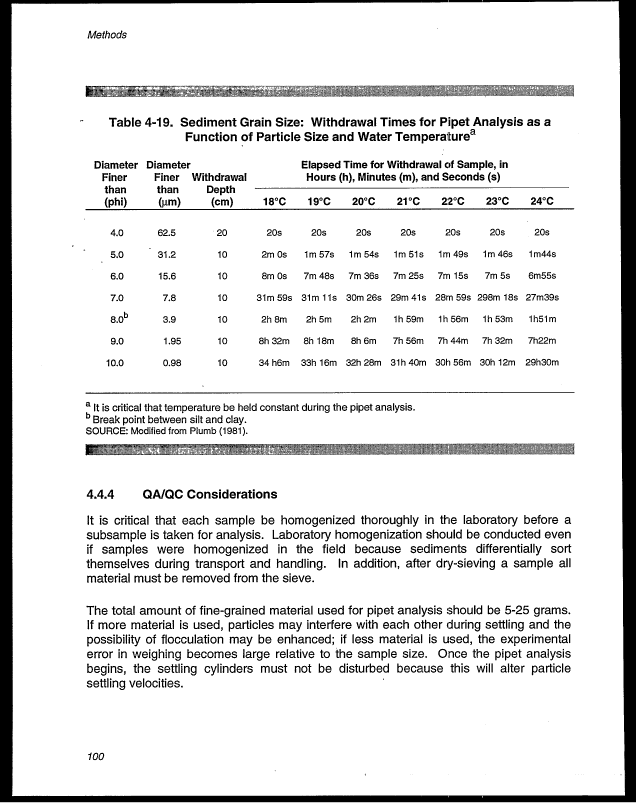
4-19. Sediment Grain Size: Withdrawal Times for Pipet Analysis as a
Function of Particle Size and Water Temperature 100
4-20. Biological Indices 115
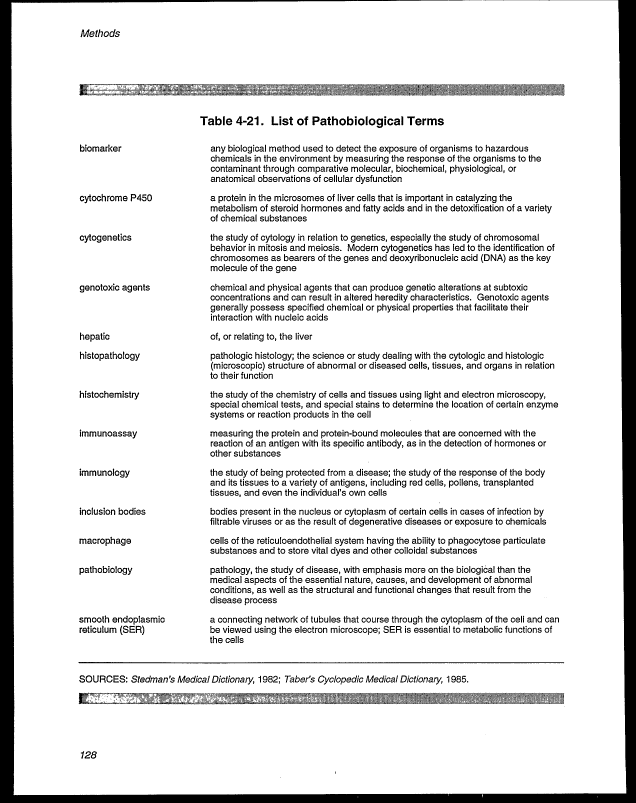
4-21. List of Pathobiological Terms 128
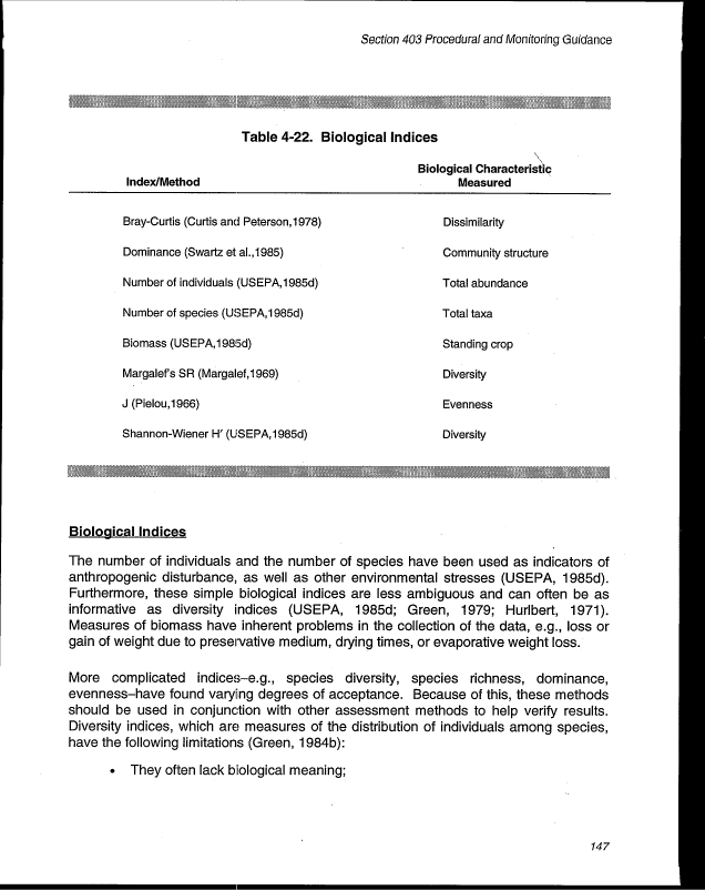
4-22. Biological Indices 147
4-23. List of Analytical Methods 167
4-24. List of Terms „ 175
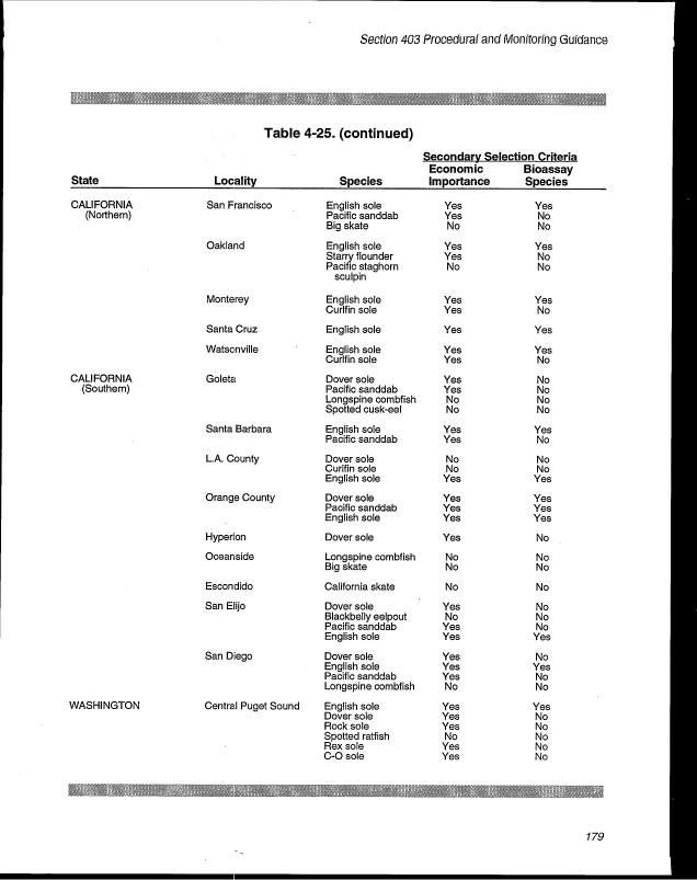
4-25. Highest-Ranking Candidate Fish for Use as Bioaccumulation
Monitoring Species 178
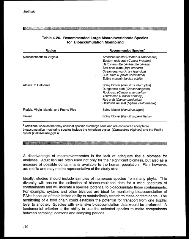
4-26. Recommended Large Macroinvertebrate Species for
Bioaccumulation Monitoring 180
4-27. List of Analytical Techniques 185
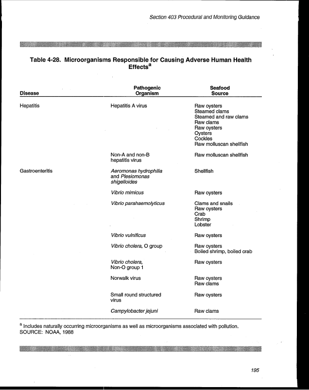
4-28. Microorganisms Responsible for Causing Adverse
Human Health Efffects 195
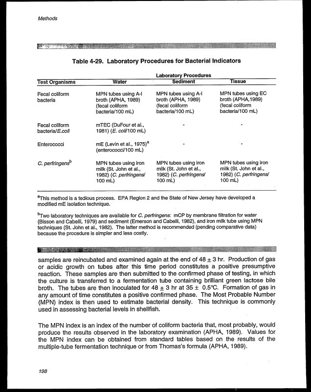
4-29. Laboratory Procedures for Bacterial Indicators 198
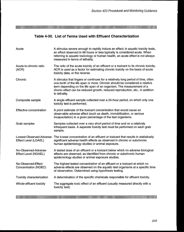
4-30. List of Terms Used with Effluent Characterization 205
image:
TABLES (continued)
Table page
4-14. List of Analytical Techniques 80
4-15. USEPA Organic Contaminant Detection Techniques 81
4-16. Summary of Quality Control Analyses 86
4-17. Summary of Warning and Control Limits for Quality Control Sample 87
4-18. Summary of Bottom Sampling Equipment 94
4-19. Sediment Grain Size: Withdrawal Times for Pipet Analysis as a
Function of Particle Size and Water Temperature 100
4-20. Biological Indices 115
4-21. List of Pathobiological Terms 128
4-22. Biological Indices 147
4-23. List of Analytical Methods 167
4-24. List of Terms „ 175
4-25. Highest-Ranking Candidate Fish for Use as Bioaccumulation
Monitoring Species 178
4-26. Recommended Large Macroinvertebrate Species for
Bioaccumulation Monitoring 180
4-27. List of Analytical Techniques 185
4-28. Microorganisms Responsible for Causing Adverse
Human Health Efffects 195
4-29. Laboratory Procedures for Bacterial Indicators 198
4-30. List of Terms Used with Effluent Characterization 205
image:
 FIGURES
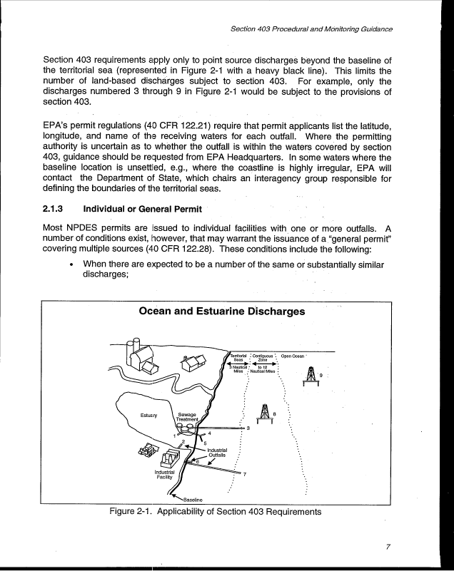
2-1. Applicability of Section 403 Requirements 7
2-2. Section 403 Decision Process 9
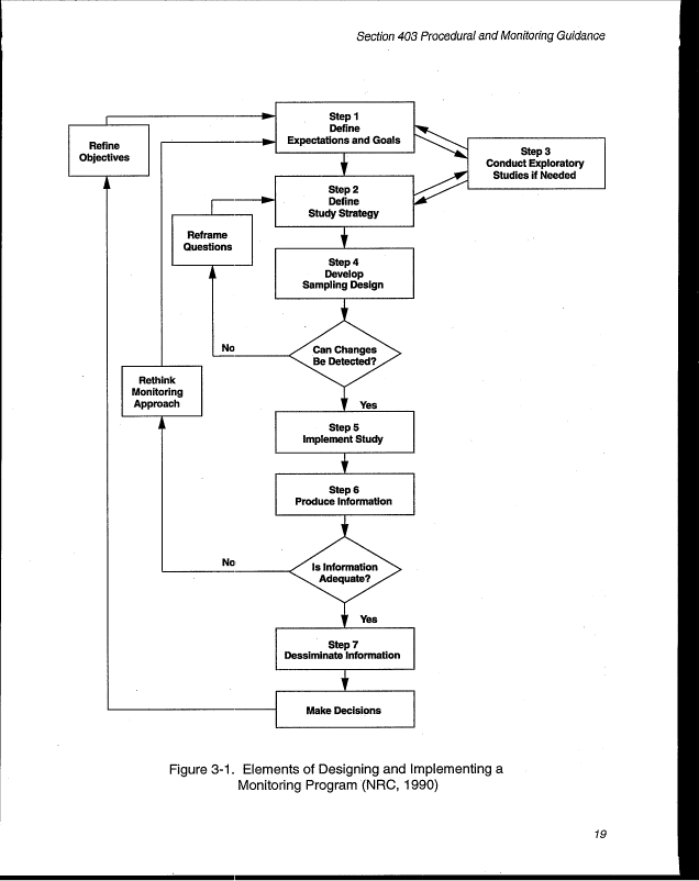
3-1. Elements of Designing and Implementing a Monitoring Program 19
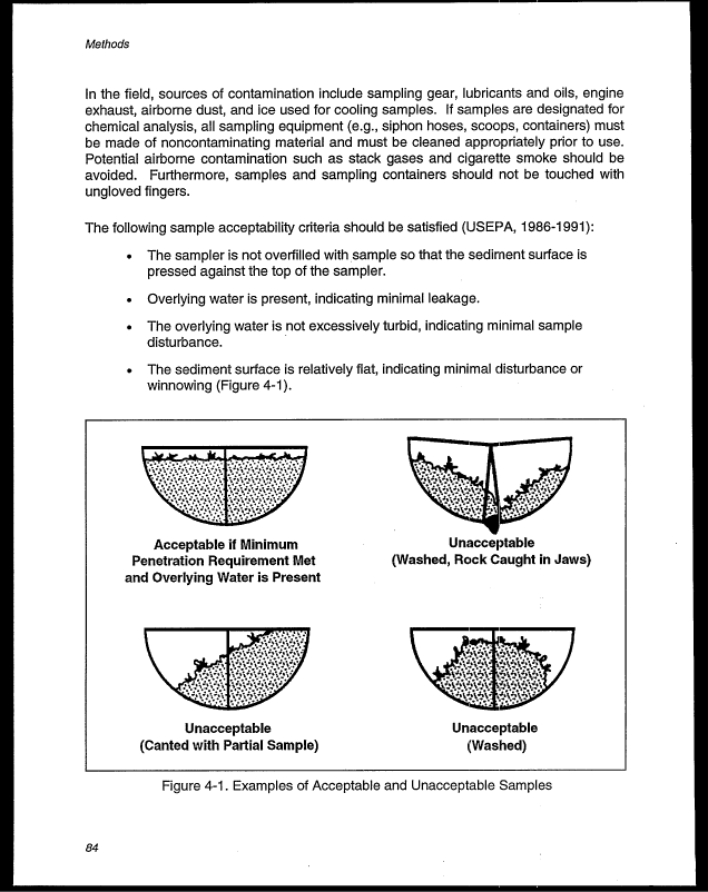
4-1. Examples of Acceptable and Unacceptable Samples 84
4-2. Generalized SAB Diagram of Changes Along a Gradient
of Organic Enrichment 117
4-3. Diagram of Changes in Fauna and Sediment Structure Along a
Gradient of Organic Enrichment 119
4-4. Examples of Acceptable and Unacceptable Samples 122
XI
image:
FIGURES
2-1. Applicability of Section 403 Requirements 7
2-2. Section 403 Decision Process 9
3-1. Elements of Designing and Implementing a Monitoring Program 19
4-1. Examples of Acceptable and Unacceptable Samples 84
4-2. Generalized SAB Diagram of Changes Along a Gradient
of Organic Enrichment 117
4-3. Diagram of Changes in Fauna and Sediment Structure Along a
Gradient of Organic Enrichment 119
4-4. Examples of Acceptable and Unacceptable Samples 122
XI
image:
 image:
 ACKNOWLEDGMENTS
This work was completed through the efforts of Brigitte Farren, National 403 Program
Coordinator; Deborah Lebow, Chief, OCPD's Marine Discharge Section; Barry Burgan,
EPA's Assessment and Watershed Protection Division; and the 403 Regional Ocean
Discharge Coordinators. For their help in the development and review of this document,
special thanks are extended to staff from EPA's Office of Research and Development,
Office of Science and Technology, and Office of Wastewater Enforcement and
Compliance. This document was prepared by Tetra Tech, Inc., under EPA Contract
Number 68-C7-0008.
XIII
image:
ACKNOWLEDGMENTS
This work was completed through the efforts of Brigitte Farren, National 403 Program
Coordinator; Deborah Lebow, Chief, OCPD's Marine Discharge Section; Barry Burgan,
EPA's Assessment and Watershed Protection Division; and the 403 Regional Ocean
Discharge Coordinators. For their help in the development and review of this document,
special thanks are extended to staff from EPA's Office of Research and Development,
Office of Science and Technology, and Office of Wastewater Enforcement and
Compliance. This document was prepared by Tetra Tech, Inc., under EPA Contract
Number 68-C7-0008.
XIII
image:
 image:
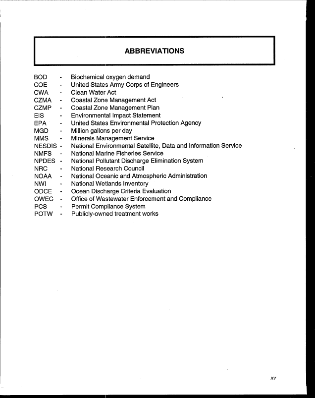
 ABBREVIATIONS
BOD - Biochemical oxygen demand
COE - United States Army Corps of Engineers
CWA - Clean Water Act
CZMA - Coastal Zone Management Act
CZMP - Coastal Zone Management Plan
EIS - Environmental Impact Statement
EPA - United States Environmental Protection Agency
MGD - Million gallons per day
MMS - Minerals Management Service
NESDIS - National Environmental Satellite, Data and Information Service
NMFS - National Marine Fisheries Service
NPDES - National Pollutant Discharge Elimination System
NRC - National Research Council
NOAA - National Oceanic and Atmospheric Administration
NWI - National Wetlands Inventory
ODCE - Ocean Discharge Criteria Evaluation
OWEC - Office of Wastewater Enforcement and Compliance
PCS - Permit Compliance System
POTW - Publicly-owned treatment works
XV
image:
ABBREVIATIONS
BOD - Biochemical oxygen demand
COE - United States Army Corps of Engineers
CWA - Clean Water Act
CZMA - Coastal Zone Management Act
CZMP - Coastal Zone Management Plan
EIS - Environmental Impact Statement
EPA - United States Environmental Protection Agency
MGD - Million gallons per day
MMS - Minerals Management Service
NESDIS - National Environmental Satellite, Data and Information Service
NMFS - National Marine Fisheries Service
NPDES - National Pollutant Discharge Elimination System
NRC - National Research Council
NOAA - National Oceanic and Atmospheric Administration
NWI - National Wetlands Inventory
ODCE - Ocean Discharge Criteria Evaluation
OWEC - Office of Wastewater Enforcement and Compliance
PCS - Permit Compliance System
POTW - Publicly-owned treatment works
XV
image:
 image:
 GLOSSARY
Acute - A stimulus severe enough to rapidly induce an effect; in aquatic toxicity tests,
an effect observed in 96 hours or less typically is considered acute. When
referring to aquatic toxicology or human health, an acute effect is not always
measured in terms of lethality.
Acute-to-chronic ratio (ACR) - The ratio of the acute toxicity of an effluent or a
toxicant to its chronic toxicity. ACR is used as a factor for estimating chronip
toxicity on the basis of acute toxicity data, or for estimating acute toxicity on the
basis of chronic toxicity data.
Alternatives assessment - An assessment of the relative impacts (economic, social,
and environmental) of on-site effluent discharge versus discharge to an
alternative site, land disposal, or another waste disposal alternative.
Ambient - Of or relating to a condition of the environment, such as temperature or
pressure, that surrounds a body or object.
Anadromous fish - Fish that spend their adult life in the sea but swim upriver to
freshwater spawning grounds to reproduce.
Analyte - The substance being identified and measured in an analysis.
Anoxic - Lack of oxygen.
Anthropogenic - Caused or influenced by the activities of humans.
Baseline - Defines the landward boundary of the territorial seas.
Benthic - Of, relating to, or occurring at the bottom of a waterbody.
Benthic biota - A form of aquatic plant or animal life that is found on or near the
bottom of a body of water.
Bioaccumulation - Process by which a compound is taken up by an aquatic
organism, both from water and through food.
XVII
image:
GLOSSARY
Acute - A stimulus severe enough to rapidly induce an effect; in aquatic toxicity tests,
an effect observed in 96 hours or less typically is considered acute. When
referring to aquatic toxicology or human health, an acute effect is not always
measured in terms of lethality.
Acute-to-chronic ratio (ACR) - The ratio of the acute toxicity of an effluent or a
toxicant to its chronic toxicity. ACR is used as a factor for estimating chronip
toxicity on the basis of acute toxicity data, or for estimating acute toxicity on the
basis of chronic toxicity data.
Alternatives assessment - An assessment of the relative impacts (economic, social,
and environmental) of on-site effluent discharge versus discharge to an
alternative site, land disposal, or another waste disposal alternative.
Ambient - Of or relating to a condition of the environment, such as temperature or
pressure, that surrounds a body or object.
Anadromous fish - Fish that spend their adult life in the sea but swim upriver to
freshwater spawning grounds to reproduce.
Analyte - The substance being identified and measured in an analysis.
Anoxic - Lack of oxygen.
Anthropogenic - Caused or influenced by the activities of humans.
Baseline - Defines the landward boundary of the territorial seas.
Benthic - Of, relating to, or occurring at the bottom of a waterbody.
Benthic biota - A form of aquatic plant or animal life that is found on or near the
bottom of a body of water.
Bioaccumulation - Process by which a compound is taken up by an aquatic
organism, both from water and through food.
XVII
image:
 Glossary
Bioassay - A test used to evaluate the relative potency of a chemical or a mixture of
chemicals by comparing its effect on a living organism with the effect of a
standard preparation on the same type of organism.
Biocriteria - Narrative expressions or numeric values of the biological characteristics
of aquatic communities based on appropriate reference conditions.
Biochemical oxygen demand (BOD) - A measure of the amount of oxygen
consumed in the biological processes that break down organic matter in water.
The greater the BOD, the greater the degree of pollution.
Biogeographical - The geographical distribution of animals and plants.
Biomass - A quantitative estimate of the entire assemblage of living organisms
considered collectively and measured in terms of mass volume or energy in
calories.
Calibration - The determination of any equipment deviation from a standard source
so as to ascertain the proper correction factors.
i
Chronic - A stimulus that lingers or continues for a relatively long period of time, often
one-tenth of the life span or more. Chronic should be considered a relative term
depending on the life span of an organism. The measurement of a chronic effect
can be reduced growth, reduced reproduction, etc., in addition to lethality.
Coastal zone - Lands and waters adjacent to the coast that exert an influence on the
uses of the sea and its ecology or, inversely, whose uses and ecology are
affected by the sea.
Compensation depth - The depth at which there is just enough light to allow the
amount of oxygen produced by phytoplankton through photosynthesis to balance
the amount consumed by their respiration.
Composite sample - A single effluent sample collected over a 24-hour period, on
which only one toxicity test is performed.
Contiguous zone - Defined in section 502(9) of the Clean Water Act to be "the entire
zone established or to be established by the United States under Article 24 of the
Convention of the Territorial Sea and the Contiguous Zone."
xvlii
image:
Glossary
Bioassay - A test used to evaluate the relative potency of a chemical or a mixture of
chemicals by comparing its effect on a living organism with the effect of a
standard preparation on the same type of organism.
Biocriteria - Narrative expressions or numeric values of the biological characteristics
of aquatic communities based on appropriate reference conditions.
Biochemical oxygen demand (BOD) - A measure of the amount of oxygen
consumed in the biological processes that break down organic matter in water.
The greater the BOD, the greater the degree of pollution.
Biogeographical - The geographical distribution of animals and plants.
Biomass - A quantitative estimate of the entire assemblage of living organisms
considered collectively and measured in terms of mass volume or energy in
calories.
Calibration - The determination of any equipment deviation from a standard source
so as to ascertain the proper correction factors.
i
Chronic - A stimulus that lingers or continues for a relatively long period of time, often
one-tenth of the life span or more. Chronic should be considered a relative term
depending on the life span of an organism. The measurement of a chronic effect
can be reduced growth, reduced reproduction, etc., in addition to lethality.
Coastal zone - Lands and waters adjacent to the coast that exert an influence on the
uses of the sea and its ecology or, inversely, whose uses and ecology are
affected by the sea.
Compensation depth - The depth at which there is just enough light to allow the
amount of oxygen produced by phytoplankton through photosynthesis to balance
the amount consumed by their respiration.
Composite sample - A single effluent sample collected over a 24-hour period, on
which only one toxicity test is performed.
Contiguous zone - Defined in section 502(9) of the Clean Water Act to be "the entire
zone established or to be established by the United States under Article 24 of the
Convention of the Territorial Sea and the Contiguous Zone."
xvlii
image:
 Section 403 Procedural and Monitoring Guidance
CTD instruments - Sampling instruments that measure conductivity, temperature,
and depth.
Cytogenetic - Referring to chromosomal aberrations.
Data Quality Objectives - Specific, integrated statements and goals developed for
each data or information collection activity to ensure that the data are of the
required quantity and quality.
Drogue - A small object attached to a surface buoy to measure currents.
Effect concentration - A point estimate of the toxicant concentration that would
cause an observable adverse effect (such as death, immobilization, or serious
incapacitation) in a given percentage of the test organisms.
Effluent - Wastewater—treated or untreated—that flows out of a treatment plant,
sewer, or industrial outfall. Generally refers to wastes discharged into surface
waters.
Effluent limitation - Any restriction on quantities, rates, or concentrations of chemical,
physical, biological, and other constituents that are discharged from point sources
into waters of the United States, including navigable waters of the contiguous
zone or the ocean.
Epifaunal - Living in the surface of the sediment.
Euphotic zone - The upper layers of a lake or ocean into which sufficient sunlight
penetrates for photosynthesis (usually down to about 80 meters).
Fecal coliform bacteria - Bacteria found in the intestinal tracts of animals. They are
an indicator of possible pathogenic contamination.
Grab samples - Samples collected over a very short period of time and on a relatively
infrequent basis. A separate toxicity test must be performed on each grab
sample.
Habitat - The place where a population lives and its surroundings, both living and
nonliving.
Section 403 Procedural and Monitoring Guidance
CTD instruments - Sampling instruments that measure conductivity, temperature,
and depth.
Cytogenetic - Referring to chromosomal aberrations.
Data Quality Objectives - Specific, integrated statements and goals developed for
each data or information collection activity to ensure that the data are of the
required quantity and quality.
Drogue - A small object attached to a surface buoy to measure currents.
Effect concentration - A point estimate of the toxicant concentration that would
cause an observable adverse effect (such as death, immobilization, or serious
incapacitation) in a given percentage of the test organisms.
Effluent - Wastewater—treated or untreated—that flows out of a treatment plant,
sewer, or industrial outfall. Generally refers to wastes discharged into surface
waters.
Effluent limitation - Any restriction on quantities, rates, or concentrations of chemical,
physical, biological, and other constituents that are discharged from point sources
into waters of the United States, including navigable waters of the contiguous
zone or the ocean.
Epifaunal - Living in the surface of the sediment.
Euphotic zone - The upper layers of a lake or ocean into which sufficient sunlight
penetrates for photosynthesis (usually down to about 80 meters).
Fecal coliform bacteria - Bacteria found in the intestinal tracts of animals. They are
an indicator of possible pathogenic contamination.
Grab samples - Samples collected over a very short period of time and on a relatively
infrequent basis. A separate toxicity test must be performed on each grab
sample.
Habitat - The place where a population lives and its surroundings, both living and
nonliving.
 Hard-bottom
 habitats - Those benthic habitats such as coral reefs, rocky subtidal
areas, and "live bottom" sponge/gorgonian habitats.
XIX
image:
habitats - Those benthic habitats such as coral reefs, rocky subtidal
areas, and "live bottom" sponge/gorgonian habitats.
XIX
image:
 Glossary
Hermatypic coral - Reef-building coral.
Hypoxic conditions - A deficiency of oxygen.
Indicator species - A species whose characteristics show the presence of specific
environmental conditions.
Indigenous species - A species native to or occurring naturally in a particular region
or environment.
Industrial source - For the purpose of this report, a nonmunicipal source of
wastewater discharges.
Infaunal - Living in the sediment.
Irreparable harm - Significant undesirable effects occurring after the date of permit
issuance that will not be reversed after cessation or modification of the discharge.
(40CFR125.121(a))
In situ - In the normal or natural position.
Lipids - Fats or fat-like substances that contain aliphatic hydrocarbons, are water
insoluble, and are easily stored in the body for use as fuel.
Lowest-Observed-Adverse-Effect Level (LOAEL) - The lowest concentration of an
effluent or toxicant that results in statistically significant adverse health effects as
observed in chronic or subchronic human epidemiology studies or animal
exposure.
Marine waters - Territorial seas, the contiguous zone, and the oceans.
Mixing zone - An area where an effluent discharge undergoes initial dilution and is
extended to cover the secondary mixing in the ambient waterbody. A mixing
zone is an allocated impact zone where water quality criteria can be exceeded as
long as a number of provisions are maintained.
Municipal source - A public source of wastewater discharges.
XX
image:
Glossary
Hermatypic coral - Reef-building coral.
Hypoxic conditions - A deficiency of oxygen.
Indicator species - A species whose characteristics show the presence of specific
environmental conditions.
Indigenous species - A species native to or occurring naturally in a particular region
or environment.
Industrial source - For the purpose of this report, a nonmunicipal source of
wastewater discharges.
Infaunal - Living in the sediment.
Irreparable harm - Significant undesirable effects occurring after the date of permit
issuance that will not be reversed after cessation or modification of the discharge.
(40CFR125.121(a))
In situ - In the normal or natural position.
Lipids - Fats or fat-like substances that contain aliphatic hydrocarbons, are water
insoluble, and are easily stored in the body for use as fuel.
Lowest-Observed-Adverse-Effect Level (LOAEL) - The lowest concentration of an
effluent or toxicant that results in statistically significant adverse health effects as
observed in chronic or subchronic human epidemiology studies or animal
exposure.
Marine waters - Territorial seas, the contiguous zone, and the oceans.
Mixing zone - An area where an effluent discharge undergoes initial dilution and is
extended to cover the secondary mixing in the ambient waterbody. A mixing
zone is an allocated impact zone where water quality criteria can be exceeded as
long as a number of provisions are maintained.
Municipal source - A public source of wastewater discharges.
XX
image:
 Section 403 Procedural and Monitoring Guidance
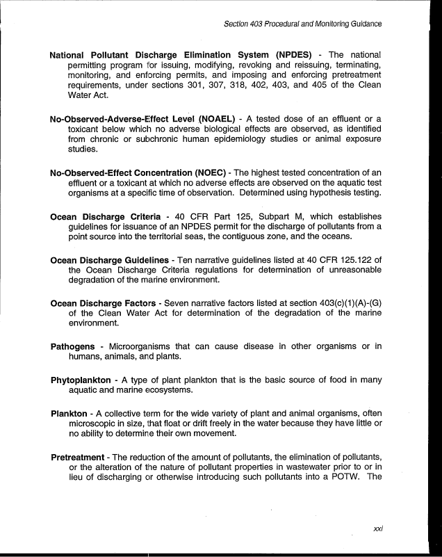
National Pollutant Discharge Elimination System (NPDES) - The national
permitting program for issuing, modifying, revoking and reissuing, terminating,
monitoring, and enforcing permits, and imposing and enforcing pretreatment
requirements, under sections 301, 307, 318, 402, 403, and 405 of the Clean
Water Act.
No-Observed-Adverse-E-ffect Level (NOAEL) - A tested dose of an effluent or a
toxicant below which no adverse biological effects are observed, as identified
from chronic or subchronic human epidemiology studies or animal exposure
studies.
No-Observed-Effect Concentration (NOEC) - The highest tested concentration of an
effluent or a toxicant at which no adverse effects are observed on the aquatic test
organisms at a specific time of observation. Determined using hypothesis testing.
Ocean Discharge Criteria - 40 CFR Part 125, Subpart M, which establishes
guidelines for issuance of an NPDES permit for the discharge of pollutants from a
point source into the territorial seas, the contiguous zone, and the oceans.
Ocean Discharge Guidelines - Ten narrative guidelines listed at 40 CFR 125.122 of
the Ocean Discharge Criteria regulations for determination of unreasonable
degradation of the marine environment.
Ocean Discharge Factors - Seven narrative factors listed at section 403(c)(1)(A)-(G)
of the Clean Water Act for determination of the degradation of the marine
environment.
Pathogens - Microorganisms that can cause disease in other organisms or in
humans, animals, and plants.
Phytoplankton - A type of plant plankton that is the basic source of food in many
aquatic and marine ecosystems.
Plankton - A collective term for the wide variety of plant and animal organisms, often
microscopic in size, that float or drift freely in the water because they have little or
no ability to determine their own movement.
Pretreatment - The reduction of the amount of pollutants, the elimination of pollutants,
or the alteration of the nature of pollutant properties in wastewater prior to or in
lieu of discharging or otherwise introducing such pollutants into a POTW. The
XXI
image:
Section 403 Procedural and Monitoring Guidance
National Pollutant Discharge Elimination System (NPDES) - The national
permitting program for issuing, modifying, revoking and reissuing, terminating,
monitoring, and enforcing permits, and imposing and enforcing pretreatment
requirements, under sections 301, 307, 318, 402, 403, and 405 of the Clean
Water Act.
No-Observed-Adverse-E-ffect Level (NOAEL) - A tested dose of an effluent or a
toxicant below which no adverse biological effects are observed, as identified
from chronic or subchronic human epidemiology studies or animal exposure
studies.
No-Observed-Effect Concentration (NOEC) - The highest tested concentration of an
effluent or a toxicant at which no adverse effects are observed on the aquatic test
organisms at a specific time of observation. Determined using hypothesis testing.
Ocean Discharge Criteria - 40 CFR Part 125, Subpart M, which establishes
guidelines for issuance of an NPDES permit for the discharge of pollutants from a
point source into the territorial seas, the contiguous zone, and the oceans.
Ocean Discharge Guidelines - Ten narrative guidelines listed at 40 CFR 125.122 of
the Ocean Discharge Criteria regulations for determination of unreasonable
degradation of the marine environment.
Ocean Discharge Factors - Seven narrative factors listed at section 403(c)(1)(A)-(G)
of the Clean Water Act for determination of the degradation of the marine
environment.
Pathogens - Microorganisms that can cause disease in other organisms or in
humans, animals, and plants.
Phytoplankton - A type of plant plankton that is the basic source of food in many
aquatic and marine ecosystems.
Plankton - A collective term for the wide variety of plant and animal organisms, often
microscopic in size, that float or drift freely in the water because they have little or
no ability to determine their own movement.
Pretreatment - The reduction of the amount of pollutants, the elimination of pollutants,
or the alteration of the nature of pollutant properties in wastewater prior to or in
lieu of discharging or otherwise introducing such pollutants into a POTW. The
XXI
image:
 Glossary
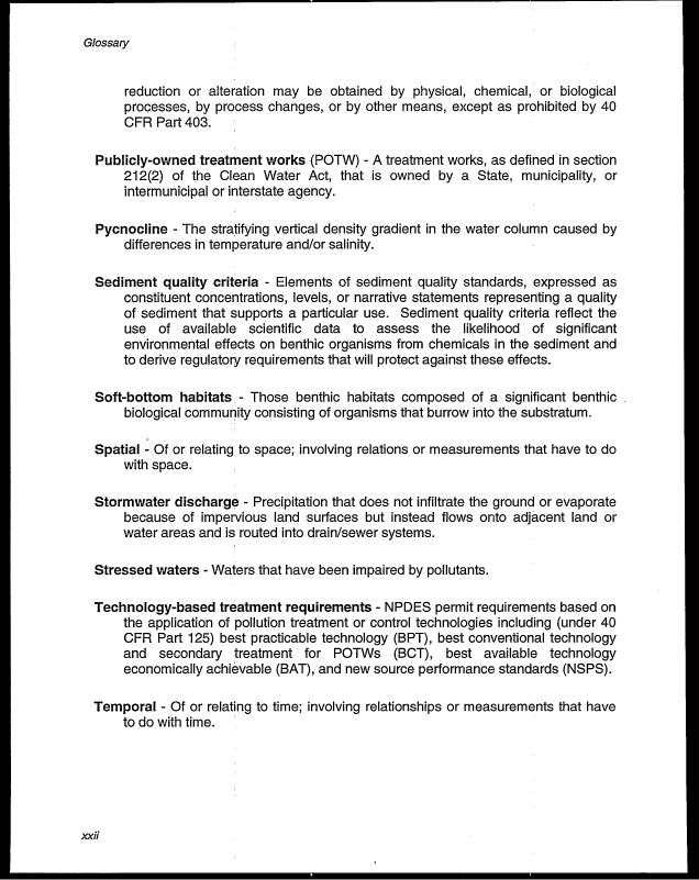
reduction or alteration may be obtained by physical, chemical, or biological
processes, by process changes, or by other means, except as prohibited by 40
CFR Part 403.
Publicly-owned treatment works (POTW) - A treatment works, as defined in section
212(2) of the Clean Water Act, that is owned by a State, municipality, or
intermunicipal or interstate agency.
Pycnocline - The stratifying vertical density gradient in the water column caused by
differences in temperature and/or salinity.
Sediment quality criteria - Elements of sediment quality standards, expressed as
constituent concentrations, levels, or narrative statements representing a quality
of sediment that supports a particular use. Sediment quality criteria reflect the
use of available scientific data to assess the likelihood of significant
environmental effects on benthic organisms from chemicals in the sediment and
to derive regulatory requirements that will protect against these effects.
Soft-bottom habitats - Those benthic habitats composed of a significant benthic
biological community consisting of organisms that burrow into the substratum.
Spatial - Of or relating to space; involving relations or measurements that have to do
with space.
Stormwater discharge - Precipitation that does not infiltrate the ground or evaporate
because of impervious land surfaces but instead flows onto adjacent land or
water areas and is routed into drain/sewer systems.
Stressed waters - Waters that have been impaired by pollutants.
Technology-based treatment requirements - NPDES permit requirements based on
the application of pollution treatment or control technologies including (under 40
CFR Part 125) best practicable technology (BPT), best conventional technology
and secondary treatment for POTWs (BCT), best available technology
economically achievable (BAT), and new source performance standards (NSPS).
Temporal - Of or relating to time; involving relationships or measurements that have
to do with time.
XXII
image:
Glossary
reduction or alteration may be obtained by physical, chemical, or biological
processes, by process changes, or by other means, except as prohibited by 40
CFR Part 403.
Publicly-owned treatment works (POTW) - A treatment works, as defined in section
212(2) of the Clean Water Act, that is owned by a State, municipality, or
intermunicipal or interstate agency.
Pycnocline - The stratifying vertical density gradient in the water column caused by
differences in temperature and/or salinity.
Sediment quality criteria - Elements of sediment quality standards, expressed as
constituent concentrations, levels, or narrative statements representing a quality
of sediment that supports a particular use. Sediment quality criteria reflect the
use of available scientific data to assess the likelihood of significant
environmental effects on benthic organisms from chemicals in the sediment and
to derive regulatory requirements that will protect against these effects.
Soft-bottom habitats - Those benthic habitats composed of a significant benthic
biological community consisting of organisms that burrow into the substratum.
Spatial - Of or relating to space; involving relations or measurements that have to do
with space.
Stormwater discharge - Precipitation that does not infiltrate the ground or evaporate
because of impervious land surfaces but instead flows onto adjacent land or
water areas and is routed into drain/sewer systems.
Stressed waters - Waters that have been impaired by pollutants.
Technology-based treatment requirements - NPDES permit requirements based on
the application of pollution treatment or control technologies including (under 40
CFR Part 125) best practicable technology (BPT), best conventional technology
and secondary treatment for POTWs (BCT), best available technology
economically achievable (BAT), and new source performance standards (NSPS).
Temporal - Of or relating to time; involving relationships or measurements that have
to do with time.
XXII
image:
 Section 403 Procedural and Monitoring Guidance
Territorial seas - Defined in section 502(8) of the Clean Water Act to be the belt of
the seas measured from the line of ordinary low water along that portion of the
coast which is in direct contact with the open sea and the line marking the
seaward limit of inland waters, and extending seaward a distance of 3 miles.
Toxic - Harmful to living organisms.
Toxicity characterization - A determination of the specific chemicals responsible for
effluent toxicity.
Toxicity test - A procedure to determine the toxicity of a chemical or an effluent using
living organisms. A toxicity test measures the degree of effect on exposed test
organisms of a specific chemical or effluent.
Unreasonable degradation - Significant adverse changes in ecosystem diversity,
productivity, and stability of the biological community within the area of discharge
and surrounding biological communities; threat to human health through direct
exposure to pollutants or through consumption of exposed aquatic organisms;
loss of aesthetic, recreational, scientific, or economic value that is unreasonable
in relation to the benefit derived from the discharge. (40 CFR 125.121 (e))
Volatile organic compounds (VOCs) - Any organic compound that participates in
atmospheric photochemical reactions.
Water quality-based toxics control - An integrated strategy used in NPDES
permitting to assess and control the discharge of toxic pollutants to surface
waters: the whole-effluent approach involving the use of toxicity tests to measure
discharge toxicity and the chemical-specific approach involving the use of water
quality criteria or State standards to limit specific toxic pollutants directly.
Water quality criteria - Elements of State water quality standards, expressed as
constituent concentrations, levels, or narrative statements, representing a quality
of water that supports a particular use. When criteria are met, water quality will
generally protect the designated use.
Water quality standards - Provisions of State or Federal law that consist of a
designated use or uses for the waters of the United States and water quality
criteria for such waters based on such uses. Water quality standards are to
protect the public health or welfare, enhance the quality of water, and serve the
purposes of the Clean Water Act.
xxm
image:
Section 403 Procedural and Monitoring Guidance
Territorial seas - Defined in section 502(8) of the Clean Water Act to be the belt of
the seas measured from the line of ordinary low water along that portion of the
coast which is in direct contact with the open sea and the line marking the
seaward limit of inland waters, and extending seaward a distance of 3 miles.
Toxic - Harmful to living organisms.
Toxicity characterization - A determination of the specific chemicals responsible for
effluent toxicity.
Toxicity test - A procedure to determine the toxicity of a chemical or an effluent using
living organisms. A toxicity test measures the degree of effect on exposed test
organisms of a specific chemical or effluent.
Unreasonable degradation - Significant adverse changes in ecosystem diversity,
productivity, and stability of the biological community within the area of discharge
and surrounding biological communities; threat to human health through direct
exposure to pollutants or through consumption of exposed aquatic organisms;
loss of aesthetic, recreational, scientific, or economic value that is unreasonable
in relation to the benefit derived from the discharge. (40 CFR 125.121 (e))
Volatile organic compounds (VOCs) - Any organic compound that participates in
atmospheric photochemical reactions.
Water quality-based toxics control - An integrated strategy used in NPDES
permitting to assess and control the discharge of toxic pollutants to surface
waters: the whole-effluent approach involving the use of toxicity tests to measure
discharge toxicity and the chemical-specific approach involving the use of water
quality criteria or State standards to limit specific toxic pollutants directly.
Water quality criteria - Elements of State water quality standards, expressed as
constituent concentrations, levels, or narrative statements, representing a quality
of water that supports a particular use. When criteria are met, water quality will
generally protect the designated use.
Water quality standards - Provisions of State or Federal law that consist of a
designated use or uses for the waters of the United States and water quality
criteria for such waters based on such uses. Water quality standards are to
protect the public health or welfare, enhance the quality of water, and serve the
purposes of the Clean Water Act.
xxm
image:
 Glossary
Whole-effluent toxicity - The aggregate toxic effect of an effluent measured directly
by a toxicity test.
Zone of initial dilution (ZID) - The region of initial mixing surrounding or adjacent to
the end of an outfall pipe or diffuser ports.
Zooplankton - A type of animal plankton.
XXIV
image:
Glossary
Whole-effluent toxicity - The aggregate toxic effect of an effluent measured directly
by a toxicity test.
Zone of initial dilution (ZID) - The region of initial mixing surrounding or adjacent to
the end of an outfall pipe or diffuser ports.
Zooplankton - A type of animal plankton.
XXIV
image:
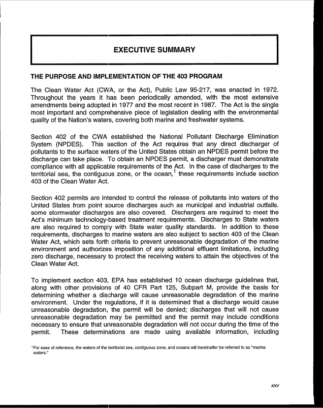
 EXECUTIVE SUMMARY
THE PURPOSE AND IMPLEMENTATION OF THE 403 PROGRAM
The Clean Water Act (CWA, or the Act), Public Law 95-217, was enacted in 1972.
Throughout the years it has been periodically amended, with the most extensive
amendments being adopted in 1977 and the most recent in 1987. The Act is the single
most important and comprehensive piece of legislation dealing with the environmental
quality of the Nation's waters, covering both marine and freshwater systems.
Section 402 of the CWA established the National Pollutant Discharge Elimination
System (NPDES). This section of the Act requires that any direct discharger of
pollutants to the surface waters of the United States obtain an NPDES permit before the
discharge can take place. To obtain an NPDES permit, a discharger must demonstrate
compliance with all applicable requirements of the Act. In the case of discharges to the
territorial sea, the contiguous zone, or the ocean,1 these requirements include section
403 of the Clean Water Act.
Section 402 permits are intended to control the release of pollutants into waters of the
United States from point source discharges such as municipal and industrial outfalls.
some stormwater discharges are also covered. Dischargers are required to meet the
Act's minimum technology-based treatment requirements. Discharges to State waters
are also required to comply with State water quality standards. In addition to these
requirements, discharges to marine waters are also subject to section 403 of the Clean
Water Act, which sets forth criteria to prevent unreasonable degradation of the marine
environment and authorizes imposition of any additional effluent limitations, including
zero discharge, necessary to protect the receiving waters to attain the objectives of the
Clean Water Act.
To implement section 403, EPA has established 10 ocean discharge guidelines that,
along with other provisions of 40 CFR Part 125, Subpart M, provide the basis for
determining whether a discharge will cause unreasonable degradation of the marine
environment. Under the regulations, if it is determined that a discharge would cause
unreasonable degradation, the permit will be denied; discharges that will not cause
unreasonable degradation may be permitted and the permit may include conditions
necessary to ensure that unreasonable degradation will not occur during the time of the
permit. These determinations are made using available information, including
1 For ease of reference, the waters of the territorial sea, contiguous zone, and oceans will hereinafter be referred to as "marine
waters."
XXV
image:
EXECUTIVE SUMMARY
THE PURPOSE AND IMPLEMENTATION OF THE 403 PROGRAM
The Clean Water Act (CWA, or the Act), Public Law 95-217, was enacted in 1972.
Throughout the years it has been periodically amended, with the most extensive
amendments being adopted in 1977 and the most recent in 1987. The Act is the single
most important and comprehensive piece of legislation dealing with the environmental
quality of the Nation's waters, covering both marine and freshwater systems.
Section 402 of the CWA established the National Pollutant Discharge Elimination
System (NPDES). This section of the Act requires that any direct discharger of
pollutants to the surface waters of the United States obtain an NPDES permit before the
discharge can take place. To obtain an NPDES permit, a discharger must demonstrate
compliance with all applicable requirements of the Act. In the case of discharges to the
territorial sea, the contiguous zone, or the ocean,1 these requirements include section
403 of the Clean Water Act.
Section 402 permits are intended to control the release of pollutants into waters of the
United States from point source discharges such as municipal and industrial outfalls.
some stormwater discharges are also covered. Dischargers are required to meet the
Act's minimum technology-based treatment requirements. Discharges to State waters
are also required to comply with State water quality standards. In addition to these
requirements, discharges to marine waters are also subject to section 403 of the Clean
Water Act, which sets forth criteria to prevent unreasonable degradation of the marine
environment and authorizes imposition of any additional effluent limitations, including
zero discharge, necessary to protect the receiving waters to attain the objectives of the
Clean Water Act.
To implement section 403, EPA has established 10 ocean discharge guidelines that,
along with other provisions of 40 CFR Part 125, Subpart M, provide the basis for
determining whether a discharge will cause unreasonable degradation of the marine
environment. Under the regulations, if it is determined that a discharge would cause
unreasonable degradation, the permit will be denied; discharges that will not cause
unreasonable degradation may be permitted and the permit may include conditions
necessary to ensure that unreasonable degradation will not occur during the time of the
permit. These determinations are made using available information, including
1 For ease of reference, the waters of the territorial sea, contiguous zone, and oceans will hereinafter be referred to as "marine
waters."
XXV
image:
 Executive Summary
information provided by the permit applicant, relevant environmental impact statements,
section 301 (h) or other variance applications, existing technical and environmental field
studies, and EPA industrial and municipal waste surveys.
In those cases where there is insufficient information to determine whether
unreasonable degradation will occur, under 40 CFR 125.123(a) and (b), a permit will not
be issued unless (1) it can be determined that no irreparable harm will result from the
discharge, (2) there are no reasonable alternatives to the discharge, and (3) the
discharge will comply with certain permit conditions specified in the regulations. These
conditions include bioassay-based discharge limitations and monitoring to assist in
determining whether and to what extent further limitations are necessary to ensure that
the discharge does not cause unreasonable degradation.
Because of the case-specific nature of permit decision making, the review and extent of
required monitoring associated with NPDES permits issued under the provisions of
section 403 are variable. This is due to the wide range of receiving environments and
the variability of the discharge. This document provides guidance on determining the
nature and extent of monitoring studies needed to assess the impact of the discharges
on the marine environment.
USE OF THIS DOCUMENT
This document is designed to provide the EPA Regions and NPDES-authorized States
with a framework for the decision-making process for section 403 evaluations and to
provide guidance on the type and level of monitoring that should be required as part of
permit issuance under the "no irreparable harm" provisions of section 403. (Generally,
ambient monitoring is not required if a determination of "no unreasonable degradation"
is made.) The decision-making aspects of the program, such as determination of
information requirements and sufficiency of information, determination of no
unreasonable degradation, and the decision to issue/reissue or deny a permit, are
described. Options for monitoring under the basis of no irreparable harm, including
criteria for evaluating perceived potential impact and establishing monitoring
requirements to assess actual impacts, are discussed. Finally, summaries of monitoring
methods for evaluating the following parameters are provided:
• Physical characteristics, such as temperature, salinity, density, depth,
turbidity, and current velocity and direction, to characterize the water column,
to verify hydrodynamic models, and to indicate spatial and temporal
variations;
• Water chemistry to evaluate the quality of receiving waters;
• Sediment chemistry to determine pollutant levels in sediments; '.
• Sediment grain size to describe spatial and temporal changes in the benthic
community;
xxvt
image:
Executive Summary
information provided by the permit applicant, relevant environmental impact statements,
section 301 (h) or other variance applications, existing technical and environmental field
studies, and EPA industrial and municipal waste surveys.
In those cases where there is insufficient information to determine whether
unreasonable degradation will occur, under 40 CFR 125.123(a) and (b), a permit will not
be issued unless (1) it can be determined that no irreparable harm will result from the
discharge, (2) there are no reasonable alternatives to the discharge, and (3) the
discharge will comply with certain permit conditions specified in the regulations. These
conditions include bioassay-based discharge limitations and monitoring to assist in
determining whether and to what extent further limitations are necessary to ensure that
the discharge does not cause unreasonable degradation.
Because of the case-specific nature of permit decision making, the review and extent of
required monitoring associated with NPDES permits issued under the provisions of
section 403 are variable. This is due to the wide range of receiving environments and
the variability of the discharge. This document provides guidance on determining the
nature and extent of monitoring studies needed to assess the impact of the discharges
on the marine environment.
USE OF THIS DOCUMENT
This document is designed to provide the EPA Regions and NPDES-authorized States
with a framework for the decision-making process for section 403 evaluations and to
provide guidance on the type and level of monitoring that should be required as part of
permit issuance under the "no irreparable harm" provisions of section 403. (Generally,
ambient monitoring is not required if a determination of "no unreasonable degradation"
is made.) The decision-making aspects of the program, such as determination of
information requirements and sufficiency of information, determination of no
unreasonable degradation, and the decision to issue/reissue or deny a permit, are
described. Options for monitoring under the basis of no irreparable harm, including
criteria for evaluating perceived potential impact and establishing monitoring
requirements to assess actual impacts, are discussed. Finally, summaries of monitoring
methods for evaluating the following parameters are provided:
• Physical characteristics, such as temperature, salinity, density, depth,
turbidity, and current velocity and direction, to characterize the water column,
to verify hydrodynamic models, and to indicate spatial and temporal
variations;
• Water chemistry to evaluate the quality of receiving waters;
• Sediment chemistry to determine pollutant levels in sediments; '.
• Sediment grain size to describe spatial and temporal changes in the benthic
community;
xxvt
image:
 Section 403 Procedural and Monitoring Quittance
• Benthic community structure to detect and describe spatial and temporal
changes in community structure and function;
• Fish and shellfish pathobiology to provide information regarding damage or
alteration to organ systems of fish and shellfish;
• Fish and shellfish populations to detect and describe spatial and temporal
changes in the abundance, structure, and function of fish and shellfish
communities;
• Plankton characteristics including biomass, productivity, and community
structure and function, to identify the dominant species, detect short- and
long-term spatial and temporal trends, and examine the relationship between
water quality conditions and community characteristics;
• Habitat identification to determine whether pollutant-related damage will
cause long-lasting harm to sensitive marine habitats;
• Bioaccumulation to provide the link between pollutant exposure and effects;
• Pathogens to assess water conditions in the vicinity of discharges and
surrounding areas and to assess relative pathogen contributions from
permitted effluent discharges;
• Effluent characterization to predict biological impacts of an effluent prior to
discharge; and
• Mesocosms and microcosms to assess ecological impacts from marine
discharges.
Each method section contains an explanation of why the measurement of the parameter
of concern might be included as part of a 403 monitoring program, and a discussion of
monitoring design considerations, analytical methods, statistical design considerations,
the use of data generated, and quality assurance/quality control considerations.
XXVII
image:
Section 403 Procedural and Monitoring Quittance
• Benthic community structure to detect and describe spatial and temporal
changes in community structure and function;
• Fish and shellfish pathobiology to provide information regarding damage or
alteration to organ systems of fish and shellfish;
• Fish and shellfish populations to detect and describe spatial and temporal
changes in the abundance, structure, and function of fish and shellfish
communities;
• Plankton characteristics including biomass, productivity, and community
structure and function, to identify the dominant species, detect short- and
long-term spatial and temporal trends, and examine the relationship between
water quality conditions and community characteristics;
• Habitat identification to determine whether pollutant-related damage will
cause long-lasting harm to sensitive marine habitats;
• Bioaccumulation to provide the link between pollutant exposure and effects;
• Pathogens to assess water conditions in the vicinity of discharges and
surrounding areas and to assess relative pathogen contributions from
permitted effluent discharges;
• Effluent characterization to predict biological impacts of an effluent prior to
discharge; and
• Mesocosms and microcosms to assess ecological impacts from marine
discharges.
Each method section contains an explanation of why the measurement of the parameter
of concern might be included as part of a 403 monitoring program, and a discussion of
monitoring design considerations, analytical methods, statistical design considerations,
the use of data generated, and quality assurance/quality control considerations.
XXVII
image:
 image:
 1. INTRODUCTION
The Clean Water Act (CWA, or the Act), Public Law 95-217, was enacted in 1972.
Throughout the years it has been periodically amended, with the most extensive
amendments being adopted in 1977 and the most recent in 1987. The Act is the single
most important and comprehensive piece of legislation dealing with the environmental
quality of the Nation's waters, covering both marine and freshwater systems.
Section 402 of the CWA established the National Pollutant Discharge Elimination
System (NPDES). This section of the Act requires that any direct discharger of
pollutants to the surface waters of the United States obtain an NPDES permit before the
discharge can take place. To obtain an NPDES permit, a discharger must demonstrate
compliance with all applicable requirements of the Act, including section 403 (for marine
discharges). Section 402 permits are intended to control the release of pollutants into
the navigable waters of the United States from all point sources, including municipal,
industrial, and some stormwater discharges.
The regulatory framework established under section 402 provides a two-pronged
approach for controlling point source discharges. The first, reliance on
"technology-based" standards, consists of national minimum treatment requirements
based on an assessment of the achievability of control technologies by individual
categories of dischargers. The second, a "water quality-based" approach, stresses
water quality criteria, water quality standards, and the setting of pollutant effluent
limitations intended to maintain receiving surface water quality at a level sufficient to
protect classified designated uses of the receiving waterbody (e.g., fishable/swimmable).
Discharges to marine waters are subject to additional regulatory requirements
established under section 403 of the CWA. Section 403 applies to marine discharges
under NPDES permits and allows for more stringent controls when necessary to protect
the environment. It is not restricted by engineering attainability, nor is it limited by
rigorous cost or economic restrictions when determining permit conditions. It includes
consideration of sediment as well as water column effects. It not only protects aquatic
species but also places special emphasis on unique, sensitive, or ecologically critical
species. Under section 403, EPA or an NPDES-authorized State can impose discharge
limitations or other conditions needed to attain compliance with section 403.
The Ocean Discharge Criteria implementing section 403 are intended to prevent
unreasonable degradation of the marine environment and to authorize imposition of
effluent limitations, if necessary, to achieve this goal. The Ocean Discharge Criteria
were promulgated on October 3, 1980, 45 FR 65942 (see Appendix B). The Ocean
image:
1. INTRODUCTION
The Clean Water Act (CWA, or the Act), Public Law 95-217, was enacted in 1972.
Throughout the years it has been periodically amended, with the most extensive
amendments being adopted in 1977 and the most recent in 1987. The Act is the single
most important and comprehensive piece of legislation dealing with the environmental
quality of the Nation's waters, covering both marine and freshwater systems.
Section 402 of the CWA established the National Pollutant Discharge Elimination
System (NPDES). This section of the Act requires that any direct discharger of
pollutants to the surface waters of the United States obtain an NPDES permit before the
discharge can take place. To obtain an NPDES permit, a discharger must demonstrate
compliance with all applicable requirements of the Act, including section 403 (for marine
discharges). Section 402 permits are intended to control the release of pollutants into
the navigable waters of the United States from all point sources, including municipal,
industrial, and some stormwater discharges.
The regulatory framework established under section 402 provides a two-pronged
approach for controlling point source discharges. The first, reliance on
"technology-based" standards, consists of national minimum treatment requirements
based on an assessment of the achievability of control technologies by individual
categories of dischargers. The second, a "water quality-based" approach, stresses
water quality criteria, water quality standards, and the setting of pollutant effluent
limitations intended to maintain receiving surface water quality at a level sufficient to
protect classified designated uses of the receiving waterbody (e.g., fishable/swimmable).
Discharges to marine waters are subject to additional regulatory requirements
established under section 403 of the CWA. Section 403 applies to marine discharges
under NPDES permits and allows for more stringent controls when necessary to protect
the environment. It is not restricted by engineering attainability, nor is it limited by
rigorous cost or economic restrictions when determining permit conditions. It includes
consideration of sediment as well as water column effects. It not only protects aquatic
species but also places special emphasis on unique, sensitive, or ecologically critical
species. Under section 403, EPA or an NPDES-authorized State can impose discharge
limitations or other conditions needed to attain compliance with section 403.
The Ocean Discharge Criteria implementing section 403 are intended to prevent
unreasonable degradation of the marine environment and to authorize imposition of
effluent limitations, if necessary, to achieve this goal. The Ocean Discharge Criteria
were promulgated on October 3, 1980, 45 FR 65942 (see Appendix B). The Ocean
image:
 Monitoring Options
Discharge Criteria provide flexibility for permit writers to customize permit application
requirements, effluent limitations, and reporting requirements to the specific conditions
of each individual discharger's situation in order to ensure compliance with section 403.
The criteria also ensure consistency by imposing minimum requirements in situations
where the long-term impacts of the discharge are not fully understood.
1.1
THE OCEAN DISCHARGE CRITERIA
Section 403(c)(1) of the Clean Water Act specifies seven factors that are to be included
in guidelines for determining the potential for degradation of marine waters. These
seven factors are the foundation for the 10 ocean discharge guidelines contained in the
EPA regulations and discussed in Section 2.2.3 of this document. Under these 10
guidelines and the other provisions of the Ocean Discharge Criteria, no NPDES permit
may be issued that will cause unreasonable degradation of the marine environment.
Prior to permit issuance; the director (defined as the EPA Regional Administrator or the
State Director where there is an NPDES-authorized State program, or an authorized
representative) is required to evaluate whether a proposed discharge will cause such
degradation. To make this determination, the director considers the provisions specified
in 40 CFR 125.122(a) and (b).
In cases where sufficient information is available for the director to make a determination
whether unreasonable degradation of the marine environment will occur, the director is
governed by 40 CFR ^25.123(3) and (b). Discharges that cause unreasonable
degradation are prohibited; other discharges may be permitted under conditions
necessary to ensure that unreasonable degradation will not occur during the term of the
permit.
In cases where the director is unable to determine whether unreasonable degradation
will occur, 40 CFR 125.i23(c) applies. Under this provision no discharge will be allowed
unless the director can determine that:
• No irreparable harm will result from the discharge;
• There are no reasonable alternatives to the discharge; and
• The discharge will comply with certain permit conditions, including
bioassay-based discharge limitations and monitoring requirements. These
conditions will assist in determining whether and to what extent further
limitations are necessary to ensure that the discharge does not cause
unreasonable degradaton. Pursuant to 40 CFR 125.123(d)(4), if on the basis
of new data the director determines that continued discharges may cause
unreasonable degradation of the marine environment, the permit must be
modified or revoked.
The Ocean Discharge Criteria encourage the use of any available information, in
addition to information supplied by the permit applicant, in determining the degradation
of marine waters as a result of a discharge. Therefore, the director may make a
image:
Monitoring Options
Discharge Criteria provide flexibility for permit writers to customize permit application
requirements, effluent limitations, and reporting requirements to the specific conditions
of each individual discharger's situation in order to ensure compliance with section 403.
The criteria also ensure consistency by imposing minimum requirements in situations
where the long-term impacts of the discharge are not fully understood.
1.1
THE OCEAN DISCHARGE CRITERIA
Section 403(c)(1) of the Clean Water Act specifies seven factors that are to be included
in guidelines for determining the potential for degradation of marine waters. These
seven factors are the foundation for the 10 ocean discharge guidelines contained in the
EPA regulations and discussed in Section 2.2.3 of this document. Under these 10
guidelines and the other provisions of the Ocean Discharge Criteria, no NPDES permit
may be issued that will cause unreasonable degradation of the marine environment.
Prior to permit issuance; the director (defined as the EPA Regional Administrator or the
State Director where there is an NPDES-authorized State program, or an authorized
representative) is required to evaluate whether a proposed discharge will cause such
degradation. To make this determination, the director considers the provisions specified
in 40 CFR 125.122(a) and (b).
In cases where sufficient information is available for the director to make a determination
whether unreasonable degradation of the marine environment will occur, the director is
governed by 40 CFR ^25.123(3) and (b). Discharges that cause unreasonable
degradation are prohibited; other discharges may be permitted under conditions
necessary to ensure that unreasonable degradation will not occur during the term of the
permit.
In cases where the director is unable to determine whether unreasonable degradation
will occur, 40 CFR 125.i23(c) applies. Under this provision no discharge will be allowed
unless the director can determine that:
• No irreparable harm will result from the discharge;
• There are no reasonable alternatives to the discharge; and
• The discharge will comply with certain permit conditions, including
bioassay-based discharge limitations and monitoring requirements. These
conditions will assist in determining whether and to what extent further
limitations are necessary to ensure that the discharge does not cause
unreasonable degradaton. Pursuant to 40 CFR 125.123(d)(4), if on the basis
of new data the director determines that continued discharges may cause
unreasonable degradation of the marine environment, the permit must be
modified or revoked.
The Ocean Discharge Criteria encourage the use of any available information, in
addition to information supplied by the permit applicant, in determining the degradation
of marine waters as a result of a discharge. Therefore, the director may make a
image:
 Section 403 Procedural and Monitoring Guidance
determination using information contained in relevant environmental impact statements,
section 301 (h) or other variance applications, existing technical and environmental field
studies, or EPA industrial and municipal waste surveys.
1.2
PURPOSE OF THIS DOCUMENT
Because of the difficulty and uncertainty inherent in predicting the precise impacts of
discharges on marine waters, ocean discharge permits may be issued/reissued under
the "no irreparable harm" provisions of 40 CFR 125.123(c) and, as a result, will require
monitoring studies to more precisely assess the impact of these discharges on the
marine environment. The purpose of this document is to provide the Regions and
NPDES-authorized States with a framework for the decision-making process to be
followed in making a section 403 determination and to provide them with guidance for
identifying the type and level of monitoring that should be required as part of a permit
issued under the "no irreparable harm" provisions of section 403.
1.3
DOCUMENT FORMAT
Chapter 2 of this document presents an explanation of, and procedural guidance for, the
overall process to be followed when issuing an NPDES permit in compliance with
section 403 of the Clean Waiter Act. Chapter 3 discusses options for monitoring under
the basis of "no irreparable harm." Chapter 4 presents a summary of monitoring
methods with potential applications to 403 discharges.
image:
Section 403 Procedural and Monitoring Guidance
determination using information contained in relevant environmental impact statements,
section 301 (h) or other variance applications, existing technical and environmental field
studies, or EPA industrial and municipal waste surveys.
1.2
PURPOSE OF THIS DOCUMENT
Because of the difficulty and uncertainty inherent in predicting the precise impacts of
discharges on marine waters, ocean discharge permits may be issued/reissued under
the "no irreparable harm" provisions of 40 CFR 125.123(c) and, as a result, will require
monitoring studies to more precisely assess the impact of these discharges on the
marine environment. The purpose of this document is to provide the Regions and
NPDES-authorized States with a framework for the decision-making process to be
followed in making a section 403 determination and to provide them with guidance for
identifying the type and level of monitoring that should be required as part of a permit
issued under the "no irreparable harm" provisions of section 403.
1.3
DOCUMENT FORMAT
Chapter 2 of this document presents an explanation of, and procedural guidance for, the
overall process to be followed when issuing an NPDES permit in compliance with
section 403 of the Clean Waiter Act. Chapter 3 discusses options for monitoring under
the basis of "no irreparable harm." Chapter 4 presents a summary of monitoring
methods with potential applications to 403 discharges.
image:
 image:
 2. SECTION 403 PROCEDURE
2.1
BACKGROUND
2.1.1 The Role of the Ocean Discharge Criteria in NPDES Permit issuance
The Ocean Discharge Criteria (40 CFR Part 125, Subpart M) are used in the
development of NPDES permits for the discharge of pollutants into marine waters. The
criteria are designed to protect marine resources from the impact of wastewater
discharges and to prevent unreasonable degradation of the marine environment.
Although referred to as the Ocean Discharge Criteria, they are promulgated regulations
that establish minimum requirements on discharges to marine waters. The 10
guidelines presented in the Ocean Discharge Criteria that must be considered when
reviewing a permit request under section 403 are presented in Table 2-1.
The regulations promulgated pursuant to section 403 are not a substitute for other
authorities of the Clean Water Act, but are a component of section 402 NPDES permits
and apply in addition to other applicable Clean Water Act requirements. Permittees
subject to section 403 must still comply with all other provisions of the Act including
sections 301 (technology-based effluent limitations), 303 (water quality standards), 306
(national standards of performance), and 307 (pretreatment). Permittees also may be
subject to section 311 (oil and hazardous substances) and section 312 (marine
sanitation devices).
The NPDES program is administered by EPA's Office of Wastewater Enforcement and
Compliance (OWEC); the section 403 program is administered by the Office of
Wetlands, Oceans and Watersheds (OWOW). OWOW is responsible for developing the
criteria and guidelines for ocean discharges that are subject to section 403. OWEC is
responsible for administering the NPDES permitting program. The actual NPDES
permits are issued by EPA Regional offices or, in States that have been granted NPDES
permitting authority, by the designated State environmental agency.
2.1.2 Applicability of Section 403
Point source discharges to waters of the United States are subject to the requirement to
obtain a section 402 NPDES permit. Permits for discharges seaward of the baseline of
the territorial seas must comply with the requirements of section 403. The "baseline"
typically follows the line of ordinary low water along the portion of the coast that is in
direct contact with the open sea although closing lines may be drawn straight across the
mouths of bays, in certain cases.
image:
2. SECTION 403 PROCEDURE
2.1
BACKGROUND
2.1.1 The Role of the Ocean Discharge Criteria in NPDES Permit issuance
The Ocean Discharge Criteria (40 CFR Part 125, Subpart M) are used in the
development of NPDES permits for the discharge of pollutants into marine waters. The
criteria are designed to protect marine resources from the impact of wastewater
discharges and to prevent unreasonable degradation of the marine environment.
Although referred to as the Ocean Discharge Criteria, they are promulgated regulations
that establish minimum requirements on discharges to marine waters. The 10
guidelines presented in the Ocean Discharge Criteria that must be considered when
reviewing a permit request under section 403 are presented in Table 2-1.
The regulations promulgated pursuant to section 403 are not a substitute for other
authorities of the Clean Water Act, but are a component of section 402 NPDES permits
and apply in addition to other applicable Clean Water Act requirements. Permittees
subject to section 403 must still comply with all other provisions of the Act including
sections 301 (technology-based effluent limitations), 303 (water quality standards), 306
(national standards of performance), and 307 (pretreatment). Permittees also may be
subject to section 311 (oil and hazardous substances) and section 312 (marine
sanitation devices).
The NPDES program is administered by EPA's Office of Wastewater Enforcement and
Compliance (OWEC); the section 403 program is administered by the Office of
Wetlands, Oceans and Watersheds (OWOW). OWOW is responsible for developing the
criteria and guidelines for ocean discharges that are subject to section 403. OWEC is
responsible for administering the NPDES permitting program. The actual NPDES
permits are issued by EPA Regional offices or, in States that have been granted NPDES
permitting authority, by the designated State environmental agency.
2.1.2 Applicability of Section 403
Point source discharges to waters of the United States are subject to the requirement to
obtain a section 402 NPDES permit. Permits for discharges seaward of the baseline of
the territorial seas must comply with the requirements of section 403. The "baseline"
typically follows the line of ordinary low water along the portion of the coast that is in
direct contact with the open sea although closing lines may be drawn straight across the
mouths of bays, in certain cases.
image:
 Monitoring Options
Table 2-1. Ocean Discharge Guidelines
(1) Quantities, composition, and potential bioaccumulation or persistence of
the pollutants to be discharged;
Potential transport of the pollutants by biological, physical, or chemical
processes;
(2)
(3)
Composition and vulnerability of potentially exposed biological
communities, including
- unique species or communities,
- endangered or threatened species, and
- species critical to the structure or function of the ecosystem;
(4) Importance of the receiving water area to the surrounding biological
community, e.g.,
- spawning sites,
- nursery/forage areas,
- migratory pathways, and
- areas necessary for critical life stages/functions of an organism;
(5) The existence of special aquatic sites, including (but not limited to)
- marine santuaries/refuges,
- parks,
- monuments,
- national seashores,
- wilderness areas, and
- coral reefs/seagrass beds;
Potential direct or indirect impacts on human health;
(6)
(7)
(8)
(9)
(10)
Existing or potential recreational and commercial fishing;
Any applicable requirements of an approved Coastal Zone Management
Plan (CZMP);
Such other factors relating to the effects of the discharge as may be
appropriate; and
Marine water quality criteria.
image:
Monitoring Options
Table 2-1. Ocean Discharge Guidelines
(1) Quantities, composition, and potential bioaccumulation or persistence of
the pollutants to be discharged;
Potential transport of the pollutants by biological, physical, or chemical
processes;
(2)
(3)
Composition and vulnerability of potentially exposed biological
communities, including
- unique species or communities,
- endangered or threatened species, and
- species critical to the structure or function of the ecosystem;
(4) Importance of the receiving water area to the surrounding biological
community, e.g.,
- spawning sites,
- nursery/forage areas,
- migratory pathways, and
- areas necessary for critical life stages/functions of an organism;
(5) The existence of special aquatic sites, including (but not limited to)
- marine santuaries/refuges,
- parks,
- monuments,
- national seashores,
- wilderness areas, and
- coral reefs/seagrass beds;
Potential direct or indirect impacts on human health;
(6)
(7)
(8)
(9)
(10)
Existing or potential recreational and commercial fishing;
Any applicable requirements of an approved Coastal Zone Management
Plan (CZMP);
Such other factors relating to the effects of the discharge as may be
appropriate; and
Marine water quality criteria.
image:
 Section 403 Procedural and Monitoring Guidance
Section 403 requirements apply only to point source discharges beyond the baseline of
the territorial sea (represented in Figure 2-1 with a heavy black line). This limits the
number of land-based discharges subject to section 403. For example, only the
discharges numbered 3 through 9 in Figure 2-1 would be subject to the provisions of
section 403.
EPA's permit regulations (40 CFR 122.21) require that permit applicants list the latitude,
longitude, and name of the receiving waters for each outfall. Where the permitting
authority is uncertain as to whether the outfall is within the waters covered by section
403, guidance should be requested from EPA Headquarters. In some waters where the
baseline location is unsettled, e.g., where the coastline is highly irregular, EPA will
contact the Department of State, which chairs an interagency group responsible for
defining the boundaries of the territorial seas.
2.1.3
Individual or General Permit
Most NPDES permits are issued to individual facilities with one or more outfalls. A
number of conditions exist, however, that may warrant the issuance of a "general permit"
covering multiple sources (40 CFR 122.28). These conditions include the following:
• When there are expected to be a number of the same or substantially similar
discharges;
Ocean and Estuarine Discharges
Estuary V Sewage
Treatment
jrritoria! .' Contiguous '. Open Ocean '
Seas ; Zone
Nautical to 12
Miles • Nautical Miles •
Baseline
Figure 2-1. Applicability of Section 403 Requirements
7
image:
Section 403 Procedural and Monitoring Guidance
Section 403 requirements apply only to point source discharges beyond the baseline of
the territorial sea (represented in Figure 2-1 with a heavy black line). This limits the
number of land-based discharges subject to section 403. For example, only the
discharges numbered 3 through 9 in Figure 2-1 would be subject to the provisions of
section 403.
EPA's permit regulations (40 CFR 122.21) require that permit applicants list the latitude,
longitude, and name of the receiving waters for each outfall. Where the permitting
authority is uncertain as to whether the outfall is within the waters covered by section
403, guidance should be requested from EPA Headquarters. In some waters where the
baseline location is unsettled, e.g., where the coastline is highly irregular, EPA will
contact the Department of State, which chairs an interagency group responsible for
defining the boundaries of the territorial seas.
2.1.3
Individual or General Permit
Most NPDES permits are issued to individual facilities with one or more outfalls. A
number of conditions exist, however, that may warrant the issuance of a "general permit"
covering multiple sources (40 CFR 122.28). These conditions include the following:
• When there are expected to be a number of the same or substantially similar
discharges;
Ocean and Estuarine Discharges
Estuary V Sewage
Treatment
jrritoria! .' Contiguous '. Open Ocean '
Seas ; Zone
Nautical to 12
Miles • Nautical Miles •
Baseline
Figure 2-1. Applicability of Section 403 Requirements
7
image:
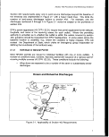 Monitoring Options
• When such discharges are expected to have the same effluent limitation
requirements; and
• When, in the opinion of the director, the discharges would be more
appropriately controlled by a general permit.
General permits may be written only if the area receiving the effluent is of a
homogenous nature; if it is circumscribed by the same geographical or political
boundary; if the uses of the receiving waters are of similar value; and if the area is not
significantly distorted by oceanographic anomalies. Examples of discharges covered
under a general permit include offshore oil and gas operations and seafood processing
operations. Exceptions to provisions of a general permit can be controlled as
subcategories within the permit as long as distinguishing features of the subcategory are
easily identified (e.g., water depth, lease block numbers).
Dischargers requesting coverage under a general permit must only notify EPA of their
intent to be covered and provide the necessary information to establish similarity to the
permitted discharges. In writing a general permit, however, EPA is the permit applicant
and must fulfill all the necessary data requirements.
2.2
GENERAL PROCEDURE
The discussion that follows presents guidance on the procedure to be followed by permit
writers when reviewing an NPDES permit request under section 403 and deciding
whether to issue such a permit and under what conditions. Once a determination has
been made that section 403 applies to a particular discharge, a general progression of
decisions is required to complete an Ocean Discharge Criteria Evaluation (ODCE).
Figure 2-2 presents the decision process that is undertaken in the review of a section
402 permit request involving ocean discharges. The discussion that follows describes
each of the steps in this process. Much of this discussion is also presented in the
preamble to the section 403 regulations (45 FR 65942, October 3,1980).
2.2.1 Request for Issuance/Reissuance of a Section 402 Permit
Any point source discharger to the navigable waters of the United States that meets the
criteria defined in section 402 of the Clean Water Act must obtain a section 402 NPDES
permit prior to discharging. In addition, any permit issued under section 402 for
discharges to marine waters must also comply with the requirements of section 403. A
permit application is submitted to the State in which the discharge occurs if the State
has been granted NPDES permitting authority by EPA. EPA processes the permit
application if the State in which the discharge occurs is not authorized or if the discharge
occurs in Federal waters (waters beyond the territorial seas).
8
image:
Monitoring Options
• When such discharges are expected to have the same effluent limitation
requirements; and
• When, in the opinion of the director, the discharges would be more
appropriately controlled by a general permit.
General permits may be written only if the area receiving the effluent is of a
homogenous nature; if it is circumscribed by the same geographical or political
boundary; if the uses of the receiving waters are of similar value; and if the area is not
significantly distorted by oceanographic anomalies. Examples of discharges covered
under a general permit include offshore oil and gas operations and seafood processing
operations. Exceptions to provisions of a general permit can be controlled as
subcategories within the permit as long as distinguishing features of the subcategory are
easily identified (e.g., water depth, lease block numbers).
Dischargers requesting coverage under a general permit must only notify EPA of their
intent to be covered and provide the necessary information to establish similarity to the
permitted discharges. In writing a general permit, however, EPA is the permit applicant
and must fulfill all the necessary data requirements.
2.2
GENERAL PROCEDURE
The discussion that follows presents guidance on the procedure to be followed by permit
writers when reviewing an NPDES permit request under section 403 and deciding
whether to issue such a permit and under what conditions. Once a determination has
been made that section 403 applies to a particular discharge, a general progression of
decisions is required to complete an Ocean Discharge Criteria Evaluation (ODCE).
Figure 2-2 presents the decision process that is undertaken in the review of a section
402 permit request involving ocean discharges. The discussion that follows describes
each of the steps in this process. Much of this discussion is also presented in the
preamble to the section 403 regulations (45 FR 65942, October 3,1980).
2.2.1 Request for Issuance/Reissuance of a Section 402 Permit
Any point source discharger to the navigable waters of the United States that meets the
criteria defined in section 402 of the Clean Water Act must obtain a section 402 NPDES
permit prior to discharging. In addition, any permit issued under section 402 for
discharges to marine waters must also comply with the requirements of section 403. A
permit application is submitted to the State in which the discharge occurs if the State
has been granted NPDES permitting authority by EPA. EPA processes the permit
application if the State in which the discharge occurs is not authorized or if the discharge
occurs in Federal waters (waters beyond the territorial seas).
8
image:
 Section 403 Procedural and Monitoring Guidance
Applicant submits request for issuance/
reissuance of permit and Information
necessary to evaluate potential Impacts
of discharge on the marine environment
40 CFR 125.124
Evaluation to determine unreasonable
degradation based on 40 CFR 125.122
Issue/Reissue Permit
May Require
- Effluent Limits
- Effluent Monitoring
- Environmental Monitoring
- Bioassays
- Best Management Practices
- Special Conditions
Issue/Reissue Permit
Must Require
- Effluent Limits
- Effluent Monitoring
- Environmental Monitoring
- Bioassays
- Best Management Practices
- Special Conditions
Permit Expiration
1 Unreasonable Degradation is:
(1) Significant adverse changes in ecosystem diversity, productivity and stability of the biological community within the area
of discharge and surrounding biological communities.
(2) Threat to human health through direct exposure to pollutants or through consumption of exposed aquatic organisms; or
(3) Loss of aesthetic, recreational, scientific, or economic values which is unreasonable in relation to benefit derived
from the discharge.
2 Irreparable harm is significant undesirable effects which will not be reversed after cessation or modification of the discharge.
3 Assuming other applicable requirements are met.
Figure 2-2. Section 403 Decision Process
9
image:
Section 403 Procedural and Monitoring Guidance
Applicant submits request for issuance/
reissuance of permit and Information
necessary to evaluate potential Impacts
of discharge on the marine environment
40 CFR 125.124
Evaluation to determine unreasonable
degradation based on 40 CFR 125.122
Issue/Reissue Permit
May Require
- Effluent Limits
- Effluent Monitoring
- Environmental Monitoring
- Bioassays
- Best Management Practices
- Special Conditions
Issue/Reissue Permit
Must Require
- Effluent Limits
- Effluent Monitoring
- Environmental Monitoring
- Bioassays
- Best Management Practices
- Special Conditions
Permit Expiration
1 Unreasonable Degradation is:
(1) Significant adverse changes in ecosystem diversity, productivity and stability of the biological community within the area
of discharge and surrounding biological communities.
(2) Threat to human health through direct exposure to pollutants or through consumption of exposed aquatic organisms; or
(3) Loss of aesthetic, recreational, scientific, or economic values which is unreasonable in relation to benefit derived
from the discharge.
2 Irreparable harm is significant undesirable effects which will not be reversed after cessation or modification of the discharge.
3 Assuming other applicable requirements are met.
Figure 2-2. Section 403 Decision Process
9
image:
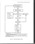 Monitoring Options
2.2.2 Determination of Information Requirements
Prior to the issuance of an NPDES permit for a discharge subject to section 403, the
director must determine that "no unreasonable degradation" of the marine environment
will occur as a result of the discharge. Such a determination is to be made after
consideration of the effects of pollutant discharge on human health and welfare, marine
life, and aesthetic, recreational, and commercial values; the persistence and
permanence of these effects; the effects of varying disposal rates; the alternative
disposal or recycling options available; and the effect on alternative uses of the ocean.
Before any decision regarding the degradation of the marine environment can be made,
the director must first determine what information is necessary to evaluate the effects of
the discharge based on the guidelines presented in the Ocean Discharge Criteria. The
director should survey the currently available information about the discharge and the
area in which the discharge would occur. This information would include the data
contained in the permit application form, as well as data available from other Agency
reports and studies.
Following a survey of currently available information, the director should determine what
additional information might be required from the applicant for the ODCE under 40 CFR
125.124. The permitting authority can require the discharger to supply information
necessary to make a determination of "no unreasonable degradation," including the
following:
• Analysis of chemical constituents of the discharge;
• Bioassays necessary to determine limiting permissible concentrations for the
discharge;
• Analysis of initial dilution;
• Process modifications that will reduce the quantities of pollutants that will be
discharged;
• Analysis of the locations where pollutants are sought to be discharged,
including biological communities, and physical description of the discharge
facility; and ;
• Evaluation of available alternatives to the discharge of pollutants, such as
land-based disposal.
The applicant is responsible for collecting the additional information and submitting it to
the director for review.
10
image:
Monitoring Options
2.2.2 Determination of Information Requirements
Prior to the issuance of an NPDES permit for a discharge subject to section 403, the
director must determine that "no unreasonable degradation" of the marine environment
will occur as a result of the discharge. Such a determination is to be made after
consideration of the effects of pollutant discharge on human health and welfare, marine
life, and aesthetic, recreational, and commercial values; the persistence and
permanence of these effects; the effects of varying disposal rates; the alternative
disposal or recycling options available; and the effect on alternative uses of the ocean.
Before any decision regarding the degradation of the marine environment can be made,
the director must first determine what information is necessary to evaluate the effects of
the discharge based on the guidelines presented in the Ocean Discharge Criteria. The
director should survey the currently available information about the discharge and the
area in which the discharge would occur. This information would include the data
contained in the permit application form, as well as data available from other Agency
reports and studies.
Following a survey of currently available information, the director should determine what
additional information might be required from the applicant for the ODCE under 40 CFR
125.124. The permitting authority can require the discharger to supply information
necessary to make a determination of "no unreasonable degradation," including the
following:
• Analysis of chemical constituents of the discharge;
• Bioassays necessary to determine limiting permissible concentrations for the
discharge;
• Analysis of initial dilution;
• Process modifications that will reduce the quantities of pollutants that will be
discharged;
• Analysis of the locations where pollutants are sought to be discharged,
including biological communities, and physical description of the discharge
facility; and ;
• Evaluation of available alternatives to the discharge of pollutants, such as
land-based disposal.
The applicant is responsible for collecting the additional information and submitting it to
the director for review.
10
image:
 Section 403 Procedural and Monitoring Guidance
2.2.3 Determination of No Unreasonable Degradation
The section 403 regulations define unreasonable degradation as
... significant adverse changes in ecosystem diversity, productivity and
stability of the biological community within the area of discharge and
surrounding biological communities, threat to human health through direct
exposure to pollutants or through consumption of exposed aquatic
organisms, or loss of aesthetic, recreational, scientific or economic values
which is unreasonable in relation to the benefit derived from the discharge.
The determination of no unreasonable degradation is to be made based on a
consideration of the 10 guidelines in 40 CFR 125.122. Discussion of these guidelines
also appears in the preamble to the section 403 regulations (45 FR 65942, October 3,
1980). The following discussion is intended to provide basic technical guidance that
might be used in determining compliance with the section 403 criteria.
(1) Quantities, composition, and potential bioaccumulation or persistence
of pollutants to be discharged. An assessment of the potential effects
of a discharge on the marine environment should carefully consider the
potential presence of persistent or toxic pollutants, especially when
present in significant quantities relative to marine water quality criteria
developed pursuant to CWA section 304(a). The potential for
bioaccumulation or persistence of pollutants in the environment is of
particular importance. In areas that do not contain sensitive species or
unusual biological communities or are not important for surrounding
biological communities, discharges containing primarily conventional
pollutants may be of lesser concern if data indicate that there will be
significant mixing with the receiving waters based on the flow of the
discharge and the physical characteristics of the discharge site, such
as water depth, density gradient, and turbulence (USEPA, 1980). An
assessment of the effluent characteristics should include the types,
sources, amounts, and temporal characteristics of the effluent, as well
as its physical, chemical, and toxicological properties and known or
demonstrated environmental impacts.
(2) Potential transport of the pollutants by biological, physical, or chemical
processes. An assessment of receiving water characteristics important
to the transport and fate of pollutants should include an evaluation of
the physical, chemical, hydrodynamic, and sedimentologic features of
the waterbody. An assessment of the biological processes that may
impact the fate and transport of contaminants and their daughter
products also may be necessary and would include consideration of
degradation through physicochemical processes, metabolic processes,
bioturbation, and potential for transport through the food chain.
11
image:
Section 403 Procedural and Monitoring Guidance
2.2.3 Determination of No Unreasonable Degradation
The section 403 regulations define unreasonable degradation as
... significant adverse changes in ecosystem diversity, productivity and
stability of the biological community within the area of discharge and
surrounding biological communities, threat to human health through direct
exposure to pollutants or through consumption of exposed aquatic
organisms, or loss of aesthetic, recreational, scientific or economic values
which is unreasonable in relation to the benefit derived from the discharge.
The determination of no unreasonable degradation is to be made based on a
consideration of the 10 guidelines in 40 CFR 125.122. Discussion of these guidelines
also appears in the preamble to the section 403 regulations (45 FR 65942, October 3,
1980). The following discussion is intended to provide basic technical guidance that
might be used in determining compliance with the section 403 criteria.
(1) Quantities, composition, and potential bioaccumulation or persistence
of pollutants to be discharged. An assessment of the potential effects
of a discharge on the marine environment should carefully consider the
potential presence of persistent or toxic pollutants, especially when
present in significant quantities relative to marine water quality criteria
developed pursuant to CWA section 304(a). The potential for
bioaccumulation or persistence of pollutants in the environment is of
particular importance. In areas that do not contain sensitive species or
unusual biological communities or are not important for surrounding
biological communities, discharges containing primarily conventional
pollutants may be of lesser concern if data indicate that there will be
significant mixing with the receiving waters based on the flow of the
discharge and the physical characteristics of the discharge site, such
as water depth, density gradient, and turbulence (USEPA, 1980). An
assessment of the effluent characteristics should include the types,
sources, amounts, and temporal characteristics of the effluent, as well
as its physical, chemical, and toxicological properties and known or
demonstrated environmental impacts.
(2) Potential transport of the pollutants by biological, physical, or chemical
processes. An assessment of receiving water characteristics important
to the transport and fate of pollutants should include an evaluation of
the physical, chemical, hydrodynamic, and sedimentologic features of
the waterbody. An assessment of the biological processes that may
impact the fate and transport of contaminants and their daughter
products also may be necessary and would include consideration of
degradation through physicochemical processes, metabolic processes,
bioturbation, and potential for transport through the food chain.
11
image:
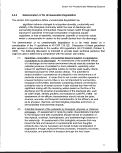 Monitoring Options
(3) Composition and vulnerability of potentially exposed biological
communities. An assessment should be made of the presence of, and
potential for, effects of a discharge on the species and biological
communities that might be impacted by the discharge. Particular
attention should be given to the possible presence of species identified
as endangered or threatened pursuant to the Endangered Species Act,
and species critical to the structure or function of the ecosystem, such
as species in food chain relationships.
(4) Importance of the receiving water area to the surrounding biological
community. The permitting authority should consider the vulnerability
of the area of discharge and its role in the larger biological community.
Environmentally significant or sensitive areas such as spawning sites,
nursery or forage areas, migratory pathways or areas necessary for
other functions or critical stages in the life cycles of organisms, areas of
high productivity, or areas under stress due to biological or climatic
conditions or discharges from other sources would be of most concern.
(5) Existence of special aquatic site. The potential for impacts on special
aquatic sites near or adjacent to the discharge should be considered.
Special aquatic sites include both those of special biological
significance and those of aesthetic or recreational importance.
Examples presented in the Ocean Discharge Criteria include:
• Marine sanctuaries,
• Refuges,
• Parks,
• National and historic monuments,
• National seashores,
• Wilderness areas, and
i
• Coral reefs.
(6) Potential direct or indirect impacts on human health. Under the 403
criteria, the permitting authority is to consider the potential impacts of
the discharge on human health, either directly through physical contact
or indirectly through the food chain. The location of the discharge, the
type and volume of the discharge's effluent, and the nature of the
surrounding biological communities should all be considered in
performing this assessment.
(7) Existing or potential recreational and commercial fishing. In
determining whether unreasonable degradation will occur, the 403
crtieria call for consideration of potential impacts on recreational and
12
image:
Monitoring Options
(3) Composition and vulnerability of potentially exposed biological
communities. An assessment should be made of the presence of, and
potential for, effects of a discharge on the species and biological
communities that might be impacted by the discharge. Particular
attention should be given to the possible presence of species identified
as endangered or threatened pursuant to the Endangered Species Act,
and species critical to the structure or function of the ecosystem, such
as species in food chain relationships.
(4) Importance of the receiving water area to the surrounding biological
community. The permitting authority should consider the vulnerability
of the area of discharge and its role in the larger biological community.
Environmentally significant or sensitive areas such as spawning sites,
nursery or forage areas, migratory pathways or areas necessary for
other functions or critical stages in the life cycles of organisms, areas of
high productivity, or areas under stress due to biological or climatic
conditions or discharges from other sources would be of most concern.
(5) Existence of special aquatic site. The potential for impacts on special
aquatic sites near or adjacent to the discharge should be considered.
Special aquatic sites include both those of special biological
significance and those of aesthetic or recreational importance.
Examples presented in the Ocean Discharge Criteria include:
• Marine sanctuaries,
• Refuges,
• Parks,
• National and historic monuments,
• National seashores,
• Wilderness areas, and
i
• Coral reefs.
(6) Potential direct or indirect impacts on human health. Under the 403
criteria, the permitting authority is to consider the potential impacts of
the discharge on human health, either directly through physical contact
or indirectly through the food chain. The location of the discharge, the
type and volume of the discharge's effluent, and the nature of the
surrounding biological communities should all be considered in
performing this assessment.
(7) Existing or potential recreational and commercial fishing. In
determining whether unreasonable degradation will occur, the 403
crtieria call for consideration of potential impacts on recreational and
12
image:
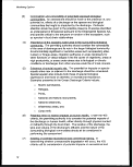 Section 403 Procedural and Monitoring Guidance
commercial fishing. This will involve identification of existing and
potential fishery resources that might be adversely affected by the
discharge and consideration of the nature and extent of these effects.
(8) Any applicable requirements of an approved Coastal Zone
Management Plan (CZMPt. The Ocean Discharge Criteria specifically
identify the need to assess the applicable requirements of an approved
State Coastal Zone Management Plan. Once a State has an approved
Coastal Zone Management Plan, the Federal consistency provisions of
section 307(c)(3) of the Coastal Zone Management Act (CZMA)
generally require that applicants for Federal licenses or permits obtain
a certification from the State as to consistency with the approved plan.
This obligation applies to NPDES permits (see 40 CFR 122.49(d)).
(9) Such other factors relating to the effects of the discharge as may be
appropriate. Permitting authorities are given the prerogative to
evaluate factors other than those specifically defined in the Ocean
Discharge Criteria when making a determination of "no unreasonable
degradation." These factors could include other statutory
requirements, impacts on other uses of the ocean such as navigation
or resource exploitation, or potential biological impacts not previously
described. The permitting authority should determine what additional
information is appropriate under given discharge circumstances and
request such information from the applicant.
(10) Marine water quality criteria. Discharges to the territorial seas are
subject to and must comply with any applicable State water quality
standards. In the absence of such State standards, or in waters
beyond a State's jurisdiction, EPA marine water quality standards
developed under section 304(a) of the CWA should be considered
when evaluating discharges. Although not binding like State water
quality standards under section 303, the EPA section 304 marine water
quality standards provide important technical information that should be
considered in performing an ODCE.
Following a review of existing information related to the 10 guidelines described above,
the permitting authority prepares an ODCE to compile and explain the information base,
conclusions, and regulator/ determinations and requirements related to a section 403
review. The ODCE should specifically address each of the 10 guidelines set out in 40
CFR 125.122 and, in general, may be organized under five broad categories of
information:
(1) Characterization of the effluent and receiving water
- discharge,
- receiving water,
- fate and transport;
13
image:
Section 403 Procedural and Monitoring Guidance
commercial fishing. This will involve identification of existing and
potential fishery resources that might be adversely affected by the
discharge and consideration of the nature and extent of these effects.
(8) Any applicable requirements of an approved Coastal Zone
Management Plan (CZMPt. The Ocean Discharge Criteria specifically
identify the need to assess the applicable requirements of an approved
State Coastal Zone Management Plan. Once a State has an approved
Coastal Zone Management Plan, the Federal consistency provisions of
section 307(c)(3) of the Coastal Zone Management Act (CZMA)
generally require that applicants for Federal licenses or permits obtain
a certification from the State as to consistency with the approved plan.
This obligation applies to NPDES permits (see 40 CFR 122.49(d)).
(9) Such other factors relating to the effects of the discharge as may be
appropriate. Permitting authorities are given the prerogative to
evaluate factors other than those specifically defined in the Ocean
Discharge Criteria when making a determination of "no unreasonable
degradation." These factors could include other statutory
requirements, impacts on other uses of the ocean such as navigation
or resource exploitation, or potential biological impacts not previously
described. The permitting authority should determine what additional
information is appropriate under given discharge circumstances and
request such information from the applicant.
(10) Marine water quality criteria. Discharges to the territorial seas are
subject to and must comply with any applicable State water quality
standards. In the absence of such State standards, or in waters
beyond a State's jurisdiction, EPA marine water quality standards
developed under section 304(a) of the CWA should be considered
when evaluating discharges. Although not binding like State water
quality standards under section 303, the EPA section 304 marine water
quality standards provide important technical information that should be
considered in performing an ODCE.
Following a review of existing information related to the 10 guidelines described above,
the permitting authority prepares an ODCE to compile and explain the information base,
conclusions, and regulator/ determinations and requirements related to a section 403
review. The ODCE should specifically address each of the 10 guidelines set out in 40
CFR 125.122 and, in general, may be organized under five broad categories of
information:
(1) Characterization of the effluent and receiving water
- discharge,
- receiving water,
- fate and transport;
13
image:
 Monitoring Options
(2) Potential effects
- aquatic life,
- human health,
- socio-economic;
(3) Other statutory/regulatory factors
- CZMA,
- Endangered Species Act,
- others (State regulations, treaties, administrative directives, etc.);
(4) Findings/Conclusions; and
(5) Regulatory outcome or actions.
A copy of the ODCE should be made available to NPDES permitting staff for inclusion as
part of the Administrative Record for the associated NPDES permit. One of three
determinations is possible after an evaluation of a discharge based on a review and
assessment of the Ocean Discharge Criteria as presented in an ODCE: (1) unreasonable
degradation will not occur; (2) unreasonable degradation will occur; or (3) insufficient
information is available to make a determination.
2.2.4 Decision to Issue/Reissue or Deny a Permit
A determination of "no unreasonable degradation" during the permit application review
process will allow the permit development and issuance process to proceed. The permit
may or may not impose further data-gathering requirements (i.e., monitoring), discharge
limitations, or other special conditions deemed necessary to prevent any future
unreasonable degradation of the marine environment. It may also include a reopener
clause. In practice, virtually all permits subject to section 403 have included reopener
clauses. If during the permit application review process a determination is made that
unreasonable degradation of the marine environment will occur, the permit will be
denied (40 CFR 125.122(b)).
2.2.5
Insufficient Information
In those cases where there is insufficient information to make a determination of "no
unreasonable degradation," under 40 CFR 125.123(c) the discharge cannot be
permitted unless three criteria are met:
(1) No irreparable harm will result from the discharge;
(2) There are no reasonable alternatives to onsite disposal; and
(3) The discharge will comply with certain mandatory permit conditions
necessary to ensure that unreasonable degradation will not occur.
14
image:
Monitoring Options
(2) Potential effects
- aquatic life,
- human health,
- socio-economic;
(3) Other statutory/regulatory factors
- CZMA,
- Endangered Species Act,
- others (State regulations, treaties, administrative directives, etc.);
(4) Findings/Conclusions; and
(5) Regulatory outcome or actions.
A copy of the ODCE should be made available to NPDES permitting staff for inclusion as
part of the Administrative Record for the associated NPDES permit. One of three
determinations is possible after an evaluation of a discharge based on a review and
assessment of the Ocean Discharge Criteria as presented in an ODCE: (1) unreasonable
degradation will not occur; (2) unreasonable degradation will occur; or (3) insufficient
information is available to make a determination.
2.2.4 Decision to Issue/Reissue or Deny a Permit
A determination of "no unreasonable degradation" during the permit application review
process will allow the permit development and issuance process to proceed. The permit
may or may not impose further data-gathering requirements (i.e., monitoring), discharge
limitations, or other special conditions deemed necessary to prevent any future
unreasonable degradation of the marine environment. It may also include a reopener
clause. In practice, virtually all permits subject to section 403 have included reopener
clauses. If during the permit application review process a determination is made that
unreasonable degradation of the marine environment will occur, the permit will be
denied (40 CFR 125.122(b)).
2.2.5
Insufficient Information
In those cases where there is insufficient information to make a determination of "no
unreasonable degradation," under 40 CFR 125.123(c) the discharge cannot be
permitted unless three criteria are met:
(1) No irreparable harm will result from the discharge;
(2) There are no reasonable alternatives to onsite disposal; and
(3) The discharge will comply with certain mandatory permit conditions
necessary to ensure that unreasonable degradation will not occur.
14
image:
 Section 403 Procedural and Monitoring Guidance
No Irreparable Harm
The first determination that must be made following a decision of "insufficient
information" is that the discharge will not cause irreparable harm to the marine
environment during the period for which the discharge will be permitted.
The Ocean Discharge Criteria define irreparable harm as "significant undesirable effects
occurring after the date of permit issuance which will not be reversed after cessation or
modification of the discharge." In evaluating the potential for irreparable harm, the
permitting authority will need to make a determination of whether the discharger,
operating pursuant to its permit conditions, will not cause permanent and significant
harm to the environment during the period in which further data on the effects of the
discharge are collected. Certain factors are particularly significant in assessing the
likelihood of irreparable harm, including the quantity of pollutants expected to be
discharged and their potential for persistence in the marine environment. An additional
factor is the sensitivity of the area into which the discharge is proposed. For example, a
discharge could cause irreparable harm to unusual and interdependent communities,
such as coral reefs and associated communities. Data on the effects of similar
discharges in similar areas are directly relevant to the determination of irreparable harm.
Information demonstrating the timely recovery of the environment after the cessation of
discharges from similar facilities would be a strong indication that irreparable harm is not
likely to occur (USEPA, 1980). In addition to considering the permanence of the
impacts, consideration must also be given to the significance of the anticipated impacts.
This would involve consideration of such factors as the areal extent of impacts, the
ecological or economic significance of affected resources, and potential impacts on
human health.
Reasonable Alternatives
If it is determined that no irreparable harm will occur as a result of a discharge, then the
second determination that inust be made prior to permitting the discharge is that there
are no reasonable alternatives (as defined in 40 CFR 125.121 (d)) to on-site disposal.
Such alternative sites would include disposal facilities located on land and discharge
points within internal waters. In determining whether a site is a reasonable alternative
to on-site disposal, the permitting authority should consider its distance from the location
of the proposed discharge and whether its use would cause unwarranted economic
impact on the discharger. The amount of material requiring disposal should also be
considered along with the availability of existing land-based disposal sites within a
reasonable distance from the point of discharge and the estimated uncommitted
capacity of such sites. A second basis for evaluating the feasibility of alternative sites is
the relative environmental harm of disposal associated with each alternative.
Alternative sites are not considered "reasonable alternatives" if on-site disposal is
judged to be environmentally preferable.
15
image:
Section 403 Procedural and Monitoring Guidance
No Irreparable Harm
The first determination that must be made following a decision of "insufficient
information" is that the discharge will not cause irreparable harm to the marine
environment during the period for which the discharge will be permitted.
The Ocean Discharge Criteria define irreparable harm as "significant undesirable effects
occurring after the date of permit issuance which will not be reversed after cessation or
modification of the discharge." In evaluating the potential for irreparable harm, the
permitting authority will need to make a determination of whether the discharger,
operating pursuant to its permit conditions, will not cause permanent and significant
harm to the environment during the period in which further data on the effects of the
discharge are collected. Certain factors are particularly significant in assessing the
likelihood of irreparable harm, including the quantity of pollutants expected to be
discharged and their potential for persistence in the marine environment. An additional
factor is the sensitivity of the area into which the discharge is proposed. For example, a
discharge could cause irreparable harm to unusual and interdependent communities,
such as coral reefs and associated communities. Data on the effects of similar
discharges in similar areas are directly relevant to the determination of irreparable harm.
Information demonstrating the timely recovery of the environment after the cessation of
discharges from similar facilities would be a strong indication that irreparable harm is not
likely to occur (USEPA, 1980). In addition to considering the permanence of the
impacts, consideration must also be given to the significance of the anticipated impacts.
This would involve consideration of such factors as the areal extent of impacts, the
ecological or economic significance of affected resources, and potential impacts on
human health.
Reasonable Alternatives
If it is determined that no irreparable harm will occur as a result of a discharge, then the
second determination that inust be made prior to permitting the discharge is that there
are no reasonable alternatives (as defined in 40 CFR 125.121 (d)) to on-site disposal.
Such alternative sites would include disposal facilities located on land and discharge
points within internal waters. In determining whether a site is a reasonable alternative
to on-site disposal, the permitting authority should consider its distance from the location
of the proposed discharge and whether its use would cause unwarranted economic
impact on the discharger. The amount of material requiring disposal should also be
considered along with the availability of existing land-based disposal sites within a
reasonable distance from the point of discharge and the estimated uncommitted
capacity of such sites. A second basis for evaluating the feasibility of alternative sites is
the relative environmental harm of disposal associated with each alternative.
Alternative sites are not considered "reasonable alternatives" if on-site disposal is
judged to be environmentally preferable.
15
image:
 Methods
Other Mandatory Permit Conditions
The final criterion for authorizing discharges for which there is insufficient information to
make a determination of "no unreasonable degradation" is that the discharge be in
compliance with all permit conditions established pursuant to §125.123(d) of the
regulations, including a bioassay-based discharge limitation {similar to those of EPA's
ocean dumping regulations, 40 CFR Part 227) and monitoring requirements. These
permit conditions are specified to assist in determining whether and to what extent
further limitations are necessary to ensure that the discharge does not cause
unreasonable degradation (USEPA, 1980).
Monitoring is required as part of a permit issued under the "no irreparable harm"
provisions of section 403. One of the principal purposes of the monitoring program is to
collect sufficient information to determine whether unreasonable degradation will occur
as a result of the discharge. Such information is then used to make a decision whether
to reissue the permit during the next round of permitting. In addition, it is vital that the
monitoring program should also be designed to ensure that no irreparable harm to the
marine environment will occur during the life of the current permit. In order to do this,
the monitoring program that is put in place must be sufficient to assess the impact of the
discharge on water, sediment, and biological quality and should include, where
appropriate, analysis of the bioaccumulative and/or persistent impact on aquatic life.
This monitoring program may include effluent analysis, bioassay analysis, and field
studies (USEPA, 1980).
It is not possible to make an a priori determination as to what constitutes an acceptable
and cost-effective monitoring program. Site-specific conditions such as the volume of
waste discharged, the types of pollutants discharged, and the location of the discharge
will play a role in determining what monitoring will be required of a discharger. These
considerations are discussed further in Chapter 3 of this document.
In addition to bioassay and monitoring requirements, the permitting authority may also
specify other permit conditions under 40 CFR 125.123(d). Seasonal restrictions on the
volume of wastes discharged can be required where such restrictions are needed to
ensure protection of the marine environment. Bioaccumulation testing of the liquid
and/or suspended particulate phase of the discharge can be required where the
potential for bioaccumulation exists, based on the nature of the pollutants discharged.
Process modifications, such as the substitution of less hazardous chemicals for those
that are potentially harmful, can be required, as can process changes that would favor
the recycling and reuse of potentially harmful pollutants.
If the data gathered pursuant to 40 CFR 125.123(d), in particular the monitoring data,
indicate that continued discharge may cause unreasonable degradation of the marine
environment, under 40 CFR 125.123(d) the permit will be revoked or modified to include
additional limitations as necessary.
16
image:
Methods
Other Mandatory Permit Conditions
The final criterion for authorizing discharges for which there is insufficient information to
make a determination of "no unreasonable degradation" is that the discharge be in
compliance with all permit conditions established pursuant to §125.123(d) of the
regulations, including a bioassay-based discharge limitation {similar to those of EPA's
ocean dumping regulations, 40 CFR Part 227) and monitoring requirements. These
permit conditions are specified to assist in determining whether and to what extent
further limitations are necessary to ensure that the discharge does not cause
unreasonable degradation (USEPA, 1980).
Monitoring is required as part of a permit issued under the "no irreparable harm"
provisions of section 403. One of the principal purposes of the monitoring program is to
collect sufficient information to determine whether unreasonable degradation will occur
as a result of the discharge. Such information is then used to make a decision whether
to reissue the permit during the next round of permitting. In addition, it is vital that the
monitoring program should also be designed to ensure that no irreparable harm to the
marine environment will occur during the life of the current permit. In order to do this,
the monitoring program that is put in place must be sufficient to assess the impact of the
discharge on water, sediment, and biological quality and should include, where
appropriate, analysis of the bioaccumulative and/or persistent impact on aquatic life.
This monitoring program may include effluent analysis, bioassay analysis, and field
studies (USEPA, 1980).
It is not possible to make an a priori determination as to what constitutes an acceptable
and cost-effective monitoring program. Site-specific conditions such as the volume of
waste discharged, the types of pollutants discharged, and the location of the discharge
will play a role in determining what monitoring will be required of a discharger. These
considerations are discussed further in Chapter 3 of this document.
In addition to bioassay and monitoring requirements, the permitting authority may also
specify other permit conditions under 40 CFR 125.123(d). Seasonal restrictions on the
volume of wastes discharged can be required where such restrictions are needed to
ensure protection of the marine environment. Bioaccumulation testing of the liquid
and/or suspended particulate phase of the discharge can be required where the
potential for bioaccumulation exists, based on the nature of the pollutants discharged.
Process modifications, such as the substitution of less hazardous chemicals for those
that are potentially harmful, can be required, as can process changes that would favor
the recycling and reuse of potentially harmful pollutants.
If the data gathered pursuant to 40 CFR 125.123(d), in particular the monitoring data,
indicate that continued discharge may cause unreasonable degradation of the marine
environment, under 40 CFR 125.123(d) the permit will be revoked or modified to include
additional limitations as necessary.
16
image:
 3. OPTIONS FOR MONITORING UNDER THE BASIS OF
"NO IRREPARABLE HARM"
3.1
BACKGROUND
The purpose of this chapter is to provide guidance to the EPA Regions and
NPDES-authorized States for determining the general types and level of monitoring that
should be required as part of a 402 permit issued or reissued under the section 403
provisions of "no irreparable harm." The guidance presented in this chapter is intended
to be used as a general assessment tool. The determination of the specific monitoring
requirements needed for a. particular discharge involves a case-by-case determination
based on the potential environmental threats posed by the particular discharge and
consideration of existing information concerning site-specific conditions. Particular
consideration should be given to the proximity of a discharge to sensitive ecological
zones, the existence of known observed biological stress based on available baseline
data for the area, discharges that have high mass emission rates and/or concentrations
of priority pollutants and other toxic substances, and the presence of other discharges in
the vicinity of the discharge in question.
A summary of methods available for conducting monitoring programs for various
environmental parameters is presented in Chapter 4. This methods summary is
presented as a guide for determining what methods are available or are being
developed. The discussion that follows in this chapter identifies only the general types
of monitoring that might be appropriate as part of a permit issued under the "no
irreparable harm" provisions of section 403. The actual monitoring requirements
specified in a 402 permit should be determined based on site-specific environmental and
discharge conditions. The references cited in Appendix A, as well as other sources,
should be referred to in the actual development and implementation of monitoring
programs.
As pointed out by the National Research Council (NRC, 1990), despite the considerable
efforts and expenditures associated with environmental monitoring, most programs fail
to provide the information needed to understand the condition of the marine environment
or to assess the effects of human activity on it. In its report Managing Troubled Waters,
the NRC (1990) identified several factors critical to the design and implementation of an
effective monitoring program. EPA suggests that the recommendations made by the
NRC be incorporated into any monitoring program required under section 403. These
recommendations include the following:
• The goals and objectives of the monitoring program need to be clearly
articulated in terms that pose questions that are meaningful to the public and
that provide the basis for scientific investigation.
17
image:
3. OPTIONS FOR MONITORING UNDER THE BASIS OF
"NO IRREPARABLE HARM"
3.1
BACKGROUND
The purpose of this chapter is to provide guidance to the EPA Regions and
NPDES-authorized States for determining the general types and level of monitoring that
should be required as part of a 402 permit issued or reissued under the section 403
provisions of "no irreparable harm." The guidance presented in this chapter is intended
to be used as a general assessment tool. The determination of the specific monitoring
requirements needed for a. particular discharge involves a case-by-case determination
based on the potential environmental threats posed by the particular discharge and
consideration of existing information concerning site-specific conditions. Particular
consideration should be given to the proximity of a discharge to sensitive ecological
zones, the existence of known observed biological stress based on available baseline
data for the area, discharges that have high mass emission rates and/or concentrations
of priority pollutants and other toxic substances, and the presence of other discharges in
the vicinity of the discharge in question.
A summary of methods available for conducting monitoring programs for various
environmental parameters is presented in Chapter 4. This methods summary is
presented as a guide for determining what methods are available or are being
developed. The discussion that follows in this chapter identifies only the general types
of monitoring that might be appropriate as part of a permit issued under the "no
irreparable harm" provisions of section 403. The actual monitoring requirements
specified in a 402 permit should be determined based on site-specific environmental and
discharge conditions. The references cited in Appendix A, as well as other sources,
should be referred to in the actual development and implementation of monitoring
programs.
As pointed out by the National Research Council (NRC, 1990), despite the considerable
efforts and expenditures associated with environmental monitoring, most programs fail
to provide the information needed to understand the condition of the marine environment
or to assess the effects of human activity on it. In its report Managing Troubled Waters,
the NRC (1990) identified several factors critical to the design and implementation of an
effective monitoring program. EPA suggests that the recommendations made by the
NRC be incorporated into any monitoring program required under section 403. These
recommendations include the following:
• The goals and objectives of the monitoring program need to be clearly
articulated in terms that pose questions that are meaningful to the public and
that provide the basis for scientific investigation.
17
image:
 Monitoring Options
• Not only must data be gathered, but attention must also be paid to their
management, synthesis, interpretation, and analysis.
• Procedures for quality assurance are needed, including scientific peer review.
• Because a well-designed monitoring program results in unanswered
questions about environmental processes or human impacts, supportive
research should be provided.
• Adequate resources are needed not only for data collection but also for
detailed analysis and evaluation over the long term.
• Programs should be sufficiently flexible to allow for their modification where
changes in conditions or new information suggests the need.
• Provision should be made to ensure that monitoring information is made
available to all interested parties in a form that is useful to them.
The central elements involved in designing and implementing an effective monitoring
program, as presented in the NRC's report (1990), are illustrated in Figure 3-1.
3.2 CRITERIA FOR EVALUATING THE POTENTIAL FOR
ENVIRONMENTAL IMPACT
To assess the potential impact posed by a discharge and thus the types and level of
monitoring that might be necessary as part of a permit issued under the "no irreparable
harm" provisions of section 403, the following site-specific determinations should be
made:
• Is the discharge in question a "major" or a "minor" discharge?
• Does the discharge occur in stressed waters?
• Does the discharge occur in the vicinity of sensitive biological areas?
• What are the number and types of other discharges in the vicinity of the
discharge in question?
3.2.1 Major/Minor Discharges
It is recommended that the Office of Wastewater Enforcement and Compliance's
(OWEC) classification of major/minor discharges be used for according such status to
discharges of concern. OWEC classifies industrial discharges as "major" or "minor"
based on an evaluation of the potential for toxic pollutant discharge, traditional pollutants
in the effluent, potential human health impacts, flow rate of effluent, and various water
quality factors. Municipal discharges are classified as "major" if ownership is public, the
facility is active, the flow rate is 1 million or more gallons per day or a population of
10,000 is served, or the discharge causes significant water quality impacts. In addition,
each EPA Region, in consultation with the environmental agency of an
NPDES-authorized State, is allowed to designate a certain percentage of its total
18
image:
Monitoring Options
• Not only must data be gathered, but attention must also be paid to their
management, synthesis, interpretation, and analysis.
• Procedures for quality assurance are needed, including scientific peer review.
• Because a well-designed monitoring program results in unanswered
questions about environmental processes or human impacts, supportive
research should be provided.
• Adequate resources are needed not only for data collection but also for
detailed analysis and evaluation over the long term.
• Programs should be sufficiently flexible to allow for their modification where
changes in conditions or new information suggests the need.
• Provision should be made to ensure that monitoring information is made
available to all interested parties in a form that is useful to them.
The central elements involved in designing and implementing an effective monitoring
program, as presented in the NRC's report (1990), are illustrated in Figure 3-1.
3.2 CRITERIA FOR EVALUATING THE POTENTIAL FOR
ENVIRONMENTAL IMPACT
To assess the potential impact posed by a discharge and thus the types and level of
monitoring that might be necessary as part of a permit issued under the "no irreparable
harm" provisions of section 403, the following site-specific determinations should be
made:
• Is the discharge in question a "major" or a "minor" discharge?
• Does the discharge occur in stressed waters?
• Does the discharge occur in the vicinity of sensitive biological areas?
• What are the number and types of other discharges in the vicinity of the
discharge in question?
3.2.1 Major/Minor Discharges
It is recommended that the Office of Wastewater Enforcement and Compliance's
(OWEC) classification of major/minor discharges be used for according such status to
discharges of concern. OWEC classifies industrial discharges as "major" or "minor"
based on an evaluation of the potential for toxic pollutant discharge, traditional pollutants
in the effluent, potential human health impacts, flow rate of effluent, and various water
quality factors. Municipal discharges are classified as "major" if ownership is public, the
facility is active, the flow rate is 1 million or more gallons per day or a population of
10,000 is served, or the discharge causes significant water quality impacts. In addition,
each EPA Region, in consultation with the environmental agency of an
NPDES-authorized State, is allowed to designate a certain percentage of its total
18
image:
 Section 403 Procedural and Monitoring Guidance
No
Step"!
Define
Expectations and Goals
Step 2
Define
Study Strategy
I
Step 4
Develop
Sampling Design
Can Changes
Be Detected?
Steps
Implement Study
I
Steps
Produce Information
Is Information
Adequate?
Yes
Step?
Dessiminate Information
I
Make Decisions
StepS
Conduct Exploratory
Studies if Needed
Figure 3-1. Elements of Designing and Implementing a
Monitoring Program (NRC, 1990)
19
image:
Section 403 Procedural and Monitoring Guidance
No
Step"!
Define
Expectations and Goals
Step 2
Define
Study Strategy
I
Step 4
Develop
Sampling Design
Can Changes
Be Detected?
Steps
Implement Study
I
Steps
Produce Information
Is Information
Adequate?
Yes
Step?
Dessiminate Information
I
Make Decisions
StepS
Conduct Exploratory
Studies if Needed
Figure 3-1. Elements of Designing and Implementing a
Monitoring Program (NRC, 1990)
19
image:
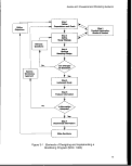 Monitoring Options
permits as "discretionary addition" major permits. This classification has been created
for those permits that the Region or State believes should be accorded major status, but
for some reason were not classified as such by OWEC.
OWEC's Permit Compliance System (PCS) is a data base management system that
tracks individual facility permit conditions. The PCS Permit Facility Data File includes
the major/minor classification for NPDES discharges.
3.2.2 Discharges to Stressed Waters
As part of the permit development process, a determination of whether a discharge
occurs in or near stressed waters should be made, and the presence of stressed waters
should be considered when determining the type and level of ambient monitoring that
should be required of a discharger. Such ambient monitoring should be designed to
determine whether and to what extent the permitted discharge is contributing to stressed
conditions and whether permit limitations are helping to alleviate such stress.
Two sources of information can be used to assess whether a discharge of concern is
occurring in stressed waters: State 305(b) reports and 304(1) lists.
Section 305(b) of the Clean Water Act requires States to report to EPA on the extent to
which their surface waters are meeting the goals of the Act and to recommend how the
goals can be achieved. Each State, territory, and Interstate Commission develops a
program to monitor the quality of its surface water and groundwater and to report the
current status of water quality to EPA in biennial Water Quality Assessment reports.
Among other things, these 305(b) reports allow EPA to:
• Determine the status of water quality;
• Identify water quality problems and trends;
• Evaluate the causes of poor water quality and the relative contributions of
pollution sources; and
• Determine the effectiveness of control programs.
In 1990, 11 States and two territories reported on the degree to which their coastal
waters support the uses for which they have been designated. This represented 4,230
coastal miles or only 22 percent of the Nation's estimated 19,200 miles of coastline.
Efforts are being made, however, to improve the 305(b) reporting process. These
improvements hopefully will result in a higher percentage of States reporting on their
coastal water quality conditions.
20
image:
Monitoring Options
permits as "discretionary addition" major permits. This classification has been created
for those permits that the Region or State believes should be accorded major status, but
for some reason were not classified as such by OWEC.
OWEC's Permit Compliance System (PCS) is a data base management system that
tracks individual facility permit conditions. The PCS Permit Facility Data File includes
the major/minor classification for NPDES discharges.
3.2.2 Discharges to Stressed Waters
As part of the permit development process, a determination of whether a discharge
occurs in or near stressed waters should be made, and the presence of stressed waters
should be considered when determining the type and level of ambient monitoring that
should be required of a discharger. Such ambient monitoring should be designed to
determine whether and to what extent the permitted discharge is contributing to stressed
conditions and whether permit limitations are helping to alleviate such stress.
Two sources of information can be used to assess whether a discharge of concern is
occurring in stressed waters: State 305(b) reports and 304(1) lists.
Section 305(b) of the Clean Water Act requires States to report to EPA on the extent to
which their surface waters are meeting the goals of the Act and to recommend how the
goals can be achieved. Each State, territory, and Interstate Commission develops a
program to monitor the quality of its surface water and groundwater and to report the
current status of water quality to EPA in biennial Water Quality Assessment reports.
Among other things, these 305(b) reports allow EPA to:
• Determine the status of water quality;
• Identify water quality problems and trends;
• Evaluate the causes of poor water quality and the relative contributions of
pollution sources; and
• Determine the effectiveness of control programs.
In 1990, 11 States and two territories reported on the degree to which their coastal
waters support the uses for which they have been designated. This represented 4,230
coastal miles or only 22 percent of the Nation's estimated 19,200 miles of coastline.
Efforts are being made, however, to improve the 305(b) reporting process. These
improvements hopefully will result in a higher percentage of States reporting on their
coastal water quality conditions.
20
image:
 Section 403 Procedural and Monitoring Guidance
Another source of information on stressed coastal waters is the State 304(1) "long list."
This is a comprehensive list of waters of the State that are impaired by point or nonpoint
source discharges of toxic, conventional, and nonconventional pollutants. Although
section 304(1) of the Clean Water Act was identified as a one-time listing of waters,
States are encouraged to maintain updated information on the status of their near
coastal waters. Unfortunately, as was the case with 305(b) reports, not all coastal
States have assessed the condition of their offshore waters.
For those coastal waters that have not been assessed by the States, a determination of
whether a discharge occurs in stressed waters should be made based on the best
professional judgment of the permitting authority using other sources of existing
information. Sources of additional information on potentially stressed waters include
EPA's 301 (h) and National Estuary programs, the Environmental Monitoring and
Assessment Program (EMAP), and the National Oceanic and Atmospheric
Administration's (NOAA) Strategic Assessment Program, as well as other
biological/ecological assessments conducted by the Federal Government (e.g., Minerals
Management Service (MMS) and U.S. Geological Survey (USGS) of the U.S.
Department of the Interior, and the U.S. Army Corps of Engineers (COE)) and State
governments.
3.2.3 Discharges to Sensitive Biological Areas
The determination of what constitutes a sensitive biological area is subject to the
discretion of the permitting authority, but at a minimum should include the following:
• Spawning sites,
• Nursery areas,
• Migratory pathways,
• Marine sanctuaries/refuges,
• Coral reefs/seagrass beds, and
• Other areas necessary for critical life stages/functions of important marine
organisms.
Numerous sources of information concerning the location of sensitive marine
environments are available. These include previous surveys conducted by State or
Federal environmental agencies. In addition to specific State environmental agencies,
major Federal sources of such information include NOAA and the U.S. Fish and Wildlife
Service (FWS) and MMS of the U.S. Department of the Interior. As part of the
information-gathering effort for an ODCE conducted for a 403 review, the discharger
should be required to investigate the existence of applicable information on sensitive
21
image:
Section 403 Procedural and Monitoring Guidance
Another source of information on stressed coastal waters is the State 304(1) "long list."
This is a comprehensive list of waters of the State that are impaired by point or nonpoint
source discharges of toxic, conventional, and nonconventional pollutants. Although
section 304(1) of the Clean Water Act was identified as a one-time listing of waters,
States are encouraged to maintain updated information on the status of their near
coastal waters. Unfortunately, as was the case with 305(b) reports, not all coastal
States have assessed the condition of their offshore waters.
For those coastal waters that have not been assessed by the States, a determination of
whether a discharge occurs in stressed waters should be made based on the best
professional judgment of the permitting authority using other sources of existing
information. Sources of additional information on potentially stressed waters include
EPA's 301 (h) and National Estuary programs, the Environmental Monitoring and
Assessment Program (EMAP), and the National Oceanic and Atmospheric
Administration's (NOAA) Strategic Assessment Program, as well as other
biological/ecological assessments conducted by the Federal Government (e.g., Minerals
Management Service (MMS) and U.S. Geological Survey (USGS) of the U.S.
Department of the Interior, and the U.S. Army Corps of Engineers (COE)) and State
governments.
3.2.3 Discharges to Sensitive Biological Areas
The determination of what constitutes a sensitive biological area is subject to the
discretion of the permitting authority, but at a minimum should include the following:
• Spawning sites,
• Nursery areas,
• Migratory pathways,
• Marine sanctuaries/refuges,
• Coral reefs/seagrass beds, and
• Other areas necessary for critical life stages/functions of important marine
organisms.
Numerous sources of information concerning the location of sensitive marine
environments are available. These include previous surveys conducted by State or
Federal environmental agencies. In addition to specific State environmental agencies,
major Federal sources of such information include NOAA and the U.S. Fish and Wildlife
Service (FWS) and MMS of the U.S. Department of the Interior. As part of the
information-gathering effort for an ODCE conducted for a 403 review, the discharger
should be required to investigate the existence of applicable information on sensitive
21
image:
 Monitoring Options
marine environments developed by these and other sources. Table 3-1 lists various
sources in NOAA, FWS, and MMS for information regarding sensitive marine
environments.
Several programs within NOAA compile information on important and sensitive marine
habitats. NOAA's National Environmental Satellite, Data and Information Service
(NESDIS) maintains an archive of worldwide data on the physical and chemical
properties of the ocean. Over the past decade, NESDIS has received large amounts
of physical, chemical, and biological data collected within the U.S. Exclusive Economic
Zone. These data derive primarily from programs organized to study the effects of
offshore oil development, ocean dumping, and other human activities on marine
ecosystems. NOAA's National Marine Sanctuary program has the responsibility of
preserving and restoring the conservation, recreational, ecological, or aesthetic values
of designated marine sanctuaries. The program presently manages seven national
marine sanctuary sites. The National Marine Fisheries Service (NMFS) of NOAA can
provide information concerning the presence of spawning and nursery sites for
important commercial and recreational fisheries, as well as information on catch of
particular species in State and Federal offshore waters. NMFS also has
responsibility for the management of some marine mammals under the Marine
Mammal Protection Act of 1972; the FWS has management responsibility for others,
including endangered species. Together, these two agencies have compiled
considerable information on marine mammal populations, life cycles, and habitat
requirements.
The FWS collects and interprets diverse information on fish and wildlife species,
populations, and habitats. Included under the management responsibility of the FWS
are anadromous fish species and endangered species, as well as some marine
mammals. The FWS publishes ecological characterization studies and species profiles
for numerous marine/estuarine fishery species. The FWS is also responsible for
producing detailed wetland maps for the contiguous United States. The mapping of
coastal wetlands has been an ongoing effort of the National Wetlands Inventory (NWI)
program at FWS. Other habitat types, including submerged aquatic vegetation, rocky
shores, reefs, and intertidal softbottoms, are also depicted on NWI maps although they
are not covered as completely as the wetlands.
As part of its offshore oil and gas leasing program, the MMS has conducted numerous
environmental impact studies and other special studies to assess the environment and
potential impact of offshore oil and gas activities on marine resources in leasing areas.
These studies include in-depth evaluations of the lease area, the affected environment,
and the potential environmental consequences of offshore oil and gas activities.
22
image:
Monitoring Options
marine environments developed by these and other sources. Table 3-1 lists various
sources in NOAA, FWS, and MMS for information regarding sensitive marine
environments.
Several programs within NOAA compile information on important and sensitive marine
habitats. NOAA's National Environmental Satellite, Data and Information Service
(NESDIS) maintains an archive of worldwide data on the physical and chemical
properties of the ocean. Over the past decade, NESDIS has received large amounts
of physical, chemical, and biological data collected within the U.S. Exclusive Economic
Zone. These data derive primarily from programs organized to study the effects of
offshore oil development, ocean dumping, and other human activities on marine
ecosystems. NOAA's National Marine Sanctuary program has the responsibility of
preserving and restoring the conservation, recreational, ecological, or aesthetic values
of designated marine sanctuaries. The program presently manages seven national
marine sanctuary sites. The National Marine Fisheries Service (NMFS) of NOAA can
provide information concerning the presence of spawning and nursery sites for
important commercial and recreational fisheries, as well as information on catch of
particular species in State and Federal offshore waters. NMFS also has
responsibility for the management of some marine mammals under the Marine
Mammal Protection Act of 1972; the FWS has management responsibility for others,
including endangered species. Together, these two agencies have compiled
considerable information on marine mammal populations, life cycles, and habitat
requirements.
The FWS collects and interprets diverse information on fish and wildlife species,
populations, and habitats. Included under the management responsibility of the FWS
are anadromous fish species and endangered species, as well as some marine
mammals. The FWS publishes ecological characterization studies and species profiles
for numerous marine/estuarine fishery species. The FWS is also responsible for
producing detailed wetland maps for the contiguous United States. The mapping of
coastal wetlands has been an ongoing effort of the National Wetlands Inventory (NWI)
program at FWS. Other habitat types, including submerged aquatic vegetation, rocky
shores, reefs, and intertidal softbottoms, are also depicted on NWI maps although they
are not covered as completely as the wetlands.
As part of its offshore oil and gas leasing program, the MMS has conducted numerous
environmental impact studies and other special studies to assess the environment and
potential impact of offshore oil and gas activities on marine resources in leasing areas.
These studies include in-depth evaluations of the lease area, the affected environment,
and the potential environmental consequences of offshore oil and gas activities.
22
image:
 Section 403 Procedural and Monitoring Guidance
Table 3-1. Information Sources on Sensitive Marine and Coastal Environments:
NOAA, FWS, and MMS
NQAA
Strategic Environmental
Assessment Division
U.S. Department of Commerce
6001 Executive Boulevard
Rockville, MD 20852-3806
301/443-8843
Alaska Region
National Marine Fisheries Service/NOAA
P.O. Box21668
Juneau, AK 99802
907/586-7221
Marine and Estuarine Management Division
NOAA/N/ORM2
U.S. Department of Commerce
Washington, DC 20235
Northeast Region
National Marine Fisheries Service/NOAA
14 Elm Street, Federal Building
Gloucester, MA 01930
813/893-3141
National Oceanographic Data Center
NOAA/NESDIS E/OC21
2001 Wisconsin Ave., NW
Washington, DC 20235
202/634-7500
Northwest Region
National Marine Fisheries Service/NOAA
7600 Sand Point Way, NE
BIN C15700-Bldgl
Seattle, WA 98115-0070
206/526-6150
Southeast Region
National Marine Fisheries Service/NOAA
9450 Koger Boulevard
St. Petersburg, FL 22703
813/893-3141
FWS
Region 1
U.S. Fish and Wildlife Service
Eastside Federal Complex
911 NE 11th Avenue
Portland, OR 97232-4181
503/231-2122
Southwest Region
National Marine Fisheries Service/NOAA
300 S. Perry Street
Terminal Island, CA 90931
213/514-6196
Region 2
U.S. Fish and Wildlife Service
500 Gold Avenue, SW
Albuquerque, NM 87103
505/766-2321
23
image:
Section 403 Procedural and Monitoring Guidance
Table 3-1. Information Sources on Sensitive Marine and Coastal Environments:
NOAA, FWS, and MMS
NQAA
Strategic Environmental
Assessment Division
U.S. Department of Commerce
6001 Executive Boulevard
Rockville, MD 20852-3806
301/443-8843
Alaska Region
National Marine Fisheries Service/NOAA
P.O. Box21668
Juneau, AK 99802
907/586-7221
Marine and Estuarine Management Division
NOAA/N/ORM2
U.S. Department of Commerce
Washington, DC 20235
Northeast Region
National Marine Fisheries Service/NOAA
14 Elm Street, Federal Building
Gloucester, MA 01930
813/893-3141
National Oceanographic Data Center
NOAA/NESDIS E/OC21
2001 Wisconsin Ave., NW
Washington, DC 20235
202/634-7500
Northwest Region
National Marine Fisheries Service/NOAA
7600 Sand Point Way, NE
BIN C15700-Bldgl
Seattle, WA 98115-0070
206/526-6150
Southeast Region
National Marine Fisheries Service/NOAA
9450 Koger Boulevard
St. Petersburg, FL 22703
813/893-3141
FWS
Region 1
U.S. Fish and Wildlife Service
Eastside Federal Complex
911 NE 11th Avenue
Portland, OR 97232-4181
503/231-2122
Southwest Region
National Marine Fisheries Service/NOAA
300 S. Perry Street
Terminal Island, CA 90931
213/514-6196
Region 2
U.S. Fish and Wildlife Service
500 Gold Avenue, SW
Albuquerque, NM 87103
505/766-2321
23
image:
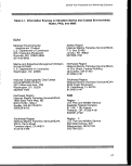 Monitoring Options
Table 3-1 (continued)
Region 4
U.S. Fish and Wildlife Service
Richard B. Russell Federal Building
75 Spring Street, SW, Room 1246
Atlanta, GA 30303
404/331-3594
Minerals Management Service
Branch of Environmental Studies (644)
Washington, DC 20240
202/343-7744
Region 5
U.S. Fish and Wildlife Service
One Gateway Center, Suite 700
Newton Corner, MA 02158
617/965-5100
Minerals Management Service
Atlantic OCS Regional Office
1951 Kidwell Dr., Suite 601
Vienna, VA 22180
703/285-2165
Region 7
U.S. Fish and Wildlife Service
1011 E.Tudor Road
Anchorage, AK 99503
970/786-3542
Minerals Management Service
Gulf of Mexico OCS Regional Office
1201 Elmwood Park Boulevard
New Orleans, LA 70123
504/736-2896
National Wetlands Inventory Program
U.S. Fish and Wildlife Service
18th and C Street, NW
Washington, DC 20240
202/235-2760
Minerals Management Service
Pacific OCS Regional Office
1340 W. 6th Street
Los Angeles, CA 90017
213/894-7120
Division of Endangered Species
U.S. Fish and Wildlife Service
4401 North Fairfax Drive, Room 452
Arlington, VA 22203
703/358-2171
Minerals Management Service
949 E. 36th Avenue, Room 110
Anchorage, AK 99508-4302
907/261-4620
Office of Management Authority
U.S. Fish and Wildlife Service
Division of Endangered Species
4401 North Fairfax Drive, Room 432
Arlington, VA 22203
703/358-2093
24
image:
Monitoring Options
Table 3-1 (continued)
Region 4
U.S. Fish and Wildlife Service
Richard B. Russell Federal Building
75 Spring Street, SW, Room 1246
Atlanta, GA 30303
404/331-3594
Minerals Management Service
Branch of Environmental Studies (644)
Washington, DC 20240
202/343-7744
Region 5
U.S. Fish and Wildlife Service
One Gateway Center, Suite 700
Newton Corner, MA 02158
617/965-5100
Minerals Management Service
Atlantic OCS Regional Office
1951 Kidwell Dr., Suite 601
Vienna, VA 22180
703/285-2165
Region 7
U.S. Fish and Wildlife Service
1011 E.Tudor Road
Anchorage, AK 99503
970/786-3542
Minerals Management Service
Gulf of Mexico OCS Regional Office
1201 Elmwood Park Boulevard
New Orleans, LA 70123
504/736-2896
National Wetlands Inventory Program
U.S. Fish and Wildlife Service
18th and C Street, NW
Washington, DC 20240
202/235-2760
Minerals Management Service
Pacific OCS Regional Office
1340 W. 6th Street
Los Angeles, CA 90017
213/894-7120
Division of Endangered Species
U.S. Fish and Wildlife Service
4401 North Fairfax Drive, Room 452
Arlington, VA 22203
703/358-2171
Minerals Management Service
949 E. 36th Avenue, Room 110
Anchorage, AK 99508-4302
907/261-4620
Office of Management Authority
U.S. Fish and Wildlife Service
Division of Endangered Species
4401 North Fairfax Drive, Room 432
Arlington, VA 22203
703/358-2093
24
image:
 Section 403 Procedural and Monitoring Guidance
3.2.4 Presence of Other Discharges in the Area
The permitting authority must determine whether the presence of other discharges in the
vicinity of the discharge of concern is likely to increase the potential for environmental
impact and thus provide justification for additional monitoring requirements. This
determination will depend on the number of other discharges in the area, their effluent
flow, and the concentration of contaminants being discharged. Although individually the
discharges in the area may not pose a significant threat to the marine environment, the
cumulative effect of numerous discharges to the same receiving waterbody could result
in a potentially significant impact on the marine environment in the vicinity of the
discharges. Consideration of the presence of other discharges occurring in the vicinity
of the discharge in question is particularly important in light of EPA's current emphasis
on watershed management.
3.3 MONITORING REQUIREMENTS BASED ON PERCEIVED POTENTIAL
ENVIRONMENTAL THREAT
Based on an evaluation of the criteria presented above, discharges can be placed into
one of three categories based on their perceived potential for causing environmental
impacts (Table 3-2):
• Minimal potential for causing environmental impacts,
• Moderate potential for causing environmental impacts, or
• High potential for causing environmental impacts.
The level and type of environmental monitoring required of a discharger will depend on
its potential for causing environmental impacts. If sufficient information is not available
to place a discharge into one of these general categories, a potential worst-case
scenario should be assumed (i.e., the discharge poses a high potential '
environmental impacts).
for
3.3.1
Minimal Potential Threat
Dischargers perceived to pose a minimal potential threat to the marine environment are
those "minor" dischargers that do not discharge to stressed waters or sensitive biological
areas and also do not discharge in the vicinity of other discharges where the combined
effects of effluents could potentially cause unacceptable cumulative impacts. The
permitting authority will have to determine the potential for cumulative impacts from
multiple discharges on a case-by-case basis.
It is recommended that discharges perceived to be of minimal potential environmental
concern be required to conduct effluent chemical characterizations, including
whole-effluent toxicity testing, and to meet aquatic life and human health water quality
criteria or standards. In addition, sediment contamination, which can involve deposition
of toxicants over long periods of time, is responsible for water quality impacts in many
25
image:
Section 403 Procedural and Monitoring Guidance
3.2.4 Presence of Other Discharges in the Area
The permitting authority must determine whether the presence of other discharges in the
vicinity of the discharge of concern is likely to increase the potential for environmental
impact and thus provide justification for additional monitoring requirements. This
determination will depend on the number of other discharges in the area, their effluent
flow, and the concentration of contaminants being discharged. Although individually the
discharges in the area may not pose a significant threat to the marine environment, the
cumulative effect of numerous discharges to the same receiving waterbody could result
in a potentially significant impact on the marine environment in the vicinity of the
discharges. Consideration of the presence of other discharges occurring in the vicinity
of the discharge in question is particularly important in light of EPA's current emphasis
on watershed management.
3.3 MONITORING REQUIREMENTS BASED ON PERCEIVED POTENTIAL
ENVIRONMENTAL THREAT
Based on an evaluation of the criteria presented above, discharges can be placed into
one of three categories based on their perceived potential for causing environmental
impacts (Table 3-2):
• Minimal potential for causing environmental impacts,
• Moderate potential for causing environmental impacts, or
• High potential for causing environmental impacts.
The level and type of environmental monitoring required of a discharger will depend on
its potential for causing environmental impacts. If sufficient information is not available
to place a discharge into one of these general categories, a potential worst-case
scenario should be assumed (i.e., the discharge poses a high potential '
environmental impacts).
for
3.3.1
Minimal Potential Threat
Dischargers perceived to pose a minimal potential threat to the marine environment are
those "minor" dischargers that do not discharge to stressed waters or sensitive biological
areas and also do not discharge in the vicinity of other discharges where the combined
effects of effluents could potentially cause unacceptable cumulative impacts. The
permitting authority will have to determine the potential for cumulative impacts from
multiple discharges on a case-by-case basis.
It is recommended that discharges perceived to be of minimal potential environmental
concern be required to conduct effluent chemical characterizations, including
whole-effluent toxicity testing, and to meet aquatic life and human health water quality
criteria or standards. In addition, sediment contamination, which can involve deposition
of toxicants over long periods of time, is responsible for water quality impacts in many
25
image:
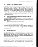 Monitoring Options
Table 3-2. Characterization of Section 403 Discharges Based on the
Potential for Causing Environmental Impacts
Potential for Causing
Environmental Impacts
Major/Minor
Discharge
Location
Rationale
Minimal
Minor
Does not occur in stressed
waters;
Does not occur in the vicinity
of sensitive habitats;
AND3
Does not occur in the vicinity
of other discharges where
the potential for cumulative
impacts exists.
Excludes high-volume and/or highly toxic
discharges.
Unreasonable degradation does not
currently appear to be a problem.
Small likelihood of impacts to recreational,
commercially, economically, or ecologically
important species.
Small likelihood of contributing to
cumulative impacts.
Moderate
Minor
Major
Occurs in stressed waters or
in the vicinity
of sensitive habitats
ORb
Occurs in the vicinity of other
discharges where the
potenital for cumulative
impacts exists.
Excludes high-volume and/or highly toxic
discharges.
In spite of low-volume and relatively nontoxic
nature of the discharge, it may be contributing
to currently stressed conditions.
May impact habitats of recreationally,
commercially, economically, or ecologically
important species that occur in the vicinity of
the discharge. !
May be contributing to cumulative impacts.
- Does not occur in stressed
waters;
- Does not occur in the vicinity
of sensitive habitats;
AND3
- Does not occur in the vicinity
of other discharges where
the potential for cumulative
impacts exists.
May include high-volume and/or highly toxic
discharges.
Unreasonable degradation does not appear
to be occurring although because of the
volume and nature of the discharge, the
potential exists.
Depending on the volume, fate, and transport
of the discharge and the toxicity and
persistence of contaminants in the effluent,
the potential exists for far-field impacts to
recreationally, commercially, economically, or
ecologically important species.
Small likelihood of contributing to cumulative
impacts.
High
Major
- Occurs in stressed waters or
in the vicinity of sensitive
habitats
ORb
- Occurs in the vicinity of other
discharges where the
potential for cumulative
impacts exists.
May include high-volume and/or highly toxic
discharges.
May be contributing to the unreasonable
degradation (i.e., stressed conditions) of the
environment.
May be contributing to cumulative impacts.
1 All conditions must be true.
' Either one or the other condition must be true.
26
image:
Monitoring Options
Table 3-2. Characterization of Section 403 Discharges Based on the
Potential for Causing Environmental Impacts
Potential for Causing
Environmental Impacts
Major/Minor
Discharge
Location
Rationale
Minimal
Minor
Does not occur in stressed
waters;
Does not occur in the vicinity
of sensitive habitats;
AND3
Does not occur in the vicinity
of other discharges where
the potential for cumulative
impacts exists.
Excludes high-volume and/or highly toxic
discharges.
Unreasonable degradation does not
currently appear to be a problem.
Small likelihood of impacts to recreational,
commercially, economically, or ecologically
important species.
Small likelihood of contributing to
cumulative impacts.
Moderate
Minor
Major
Occurs in stressed waters or
in the vicinity
of sensitive habitats
ORb
Occurs in the vicinity of other
discharges where the
potenital for cumulative
impacts exists.
Excludes high-volume and/or highly toxic
discharges.
In spite of low-volume and relatively nontoxic
nature of the discharge, it may be contributing
to currently stressed conditions.
May impact habitats of recreationally,
commercially, economically, or ecologically
important species that occur in the vicinity of
the discharge. !
May be contributing to cumulative impacts.
- Does not occur in stressed
waters;
- Does not occur in the vicinity
of sensitive habitats;
AND3
- Does not occur in the vicinity
of other discharges where
the potential for cumulative
impacts exists.
May include high-volume and/or highly toxic
discharges.
Unreasonable degradation does not appear
to be occurring although because of the
volume and nature of the discharge, the
potential exists.
Depending on the volume, fate, and transport
of the discharge and the toxicity and
persistence of contaminants in the effluent,
the potential exists for far-field impacts to
recreationally, commercially, economically, or
ecologically important species.
Small likelihood of contributing to cumulative
impacts.
High
Major
- Occurs in stressed waters or
in the vicinity of sensitive
habitats
ORb
- Occurs in the vicinity of other
discharges where the
potential for cumulative
impacts exists.
May include high-volume and/or highly toxic
discharges.
May be contributing to the unreasonable
degradation (i.e., stressed conditions) of the
environment.
May be contributing to cumulative impacts.
1 All conditions must be true.
' Either one or the other condition must be true.
26
image:
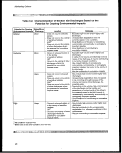 Section 403 Procedural and Monitoring Guidance
areas. Therefore, for discharges posing a minimal potential threat to the marine
environment, it is recommended that near-field sediment contamination monitoring, in
the form of sediment toxicity tests, be a requirement for 402 permits issued with 403
provisions or conditions.
3.3.2
Moderate Potential Threat
Both major and minor discharges can be considered to pose moderate potential threats
to the marine environment. Minor discharges that are discharged to stressed waters or
in the vicinity of sensitive biological areas or are discharged in the vicinity of other
discharges where the combined effects of effluents could potentially cause unacceptable
cumulative impacts should be considered to pose moderate threats to the marine
environment. Major facilities that do not discharge to stressed waters or sensitive
biological areas and that also do not discharge in the vicinity of other discharges where
the potential for cumulative Impacts exists should also be considered to pose moderate
threats to the marine environment.
For discharges posing a moderate potential threat, field monitoring (in addition to
sediment toxicity and effluent chemical characterization requirements for discharges
presumed to cause minimal environmental impacts) should be a conditional part of 402
permits issued with section 403 provisions for "no irreparable harm." Such monitoring
efforts should include physical transport studies as well as near-field measurements of
contaminant concentrations in the water column, sediment, and benthic biota.
Biosurveys and bioassessments should also be used to directly evaluate the overall
biological integrity (structure and/or functional characteristics) of the aquatic community.
Current measurements and dye studies are recommended for tracking oceanic
wastewater plumes. The purpose of such studies is to estimate the distance from the
outfall that contaminated particles may travel before accumulating on the bottom and to
evaluate the movement and spatial extent of the plume, the likelihood that the plume will
reach the shoreline or other nearby areas, and the recirculation potential under
short-term influences for existing discharges as well as the general circulation patterns
in the vicinity of discharge sites. Seasonal current measurements and dye studies
should be conducted to detect changes in current strength and direction (particularly
wind-driven currents). The effects of a storm event on transport should also be
investigated. Results of such studies can be used to identify areas potentially impacted
by the discharge and to identify existing and potential problem areas for fish and
sensitive life stages of marine organisms. Data from physical transport studies can also
be used to calibrate and validate dispersion plume models.
Near-field monitoring of chemical concentrations can provide a spatial and temporal
record of contamination in the water column. Water quality chemistry measurements
should be made as part of a monitoring program to assess the effectiveness of permit
27
image:
Section 403 Procedural and Monitoring Guidance
areas. Therefore, for discharges posing a minimal potential threat to the marine
environment, it is recommended that near-field sediment contamination monitoring, in
the form of sediment toxicity tests, be a requirement for 402 permits issued with 403
provisions or conditions.
3.3.2
Moderate Potential Threat
Both major and minor discharges can be considered to pose moderate potential threats
to the marine environment. Minor discharges that are discharged to stressed waters or
in the vicinity of sensitive biological areas or are discharged in the vicinity of other
discharges where the combined effects of effluents could potentially cause unacceptable
cumulative impacts should be considered to pose moderate threats to the marine
environment. Major facilities that do not discharge to stressed waters or sensitive
biological areas and that also do not discharge in the vicinity of other discharges where
the potential for cumulative Impacts exists should also be considered to pose moderate
threats to the marine environment.
For discharges posing a moderate potential threat, field monitoring (in addition to
sediment toxicity and effluent chemical characterization requirements for discharges
presumed to cause minimal environmental impacts) should be a conditional part of 402
permits issued with section 403 provisions for "no irreparable harm." Such monitoring
efforts should include physical transport studies as well as near-field measurements of
contaminant concentrations in the water column, sediment, and benthic biota.
Biosurveys and bioassessments should also be used to directly evaluate the overall
biological integrity (structure and/or functional characteristics) of the aquatic community.
Current measurements and dye studies are recommended for tracking oceanic
wastewater plumes. The purpose of such studies is to estimate the distance from the
outfall that contaminated particles may travel before accumulating on the bottom and to
evaluate the movement and spatial extent of the plume, the likelihood that the plume will
reach the shoreline or other nearby areas, and the recirculation potential under
short-term influences for existing discharges as well as the general circulation patterns
in the vicinity of discharge sites. Seasonal current measurements and dye studies
should be conducted to detect changes in current strength and direction (particularly
wind-driven currents). The effects of a storm event on transport should also be
investigated. Results of such studies can be used to identify areas potentially impacted
by the discharge and to identify existing and potential problem areas for fish and
sensitive life stages of marine organisms. Data from physical transport studies can also
be used to calibrate and validate dispersion plume models.
Near-field monitoring of chemical concentrations can provide a spatial and temporal
record of contamination in the water column. Water quality chemistry measurements
should be made as part of a monitoring program to assess the effectiveness of permit
27
image:
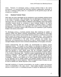 Monitoring Options
limitations in meeting water quality standards and to identify discharges that may not be
in compliance with those standards. Water quality data can also be used to calibrate
and verify mathematical models.
As discussed in the revised Technical Support Document for Water Quality-based
Toxics Control (USEPA, 1991c), EPA encourages States to develop and adopt
biological criteria in their water quality standards to fully protect aquatic habitats and
provide more comprehensive assessments to determine the nonattainment of aquatic
life uses. Biocriteria are numerical measures or narrative descriptions of the biological
integrity of unimpaired natural systems. The biological communities in these waters
become a reference and represent the best attainable conditions. The reference site
then becomes the basis for developing biocriteria for major surface water types (in this
case, coastal or marine waters). An assessment of biological integrity should include a
measure of the structure and function of a community or species within a specific
habitat. The specific definition of biological integrity selected by a State will form the
basis for comparing impacted sites to an established reference condition.
For those discharges that pose a potential moderate threat to the marine environment,
near-field biosurveys should be conducted and the results compared to reference
conditions. Such biosurveys will provide a useful monitoring of both aggregate
ecological impact and overall temporal trends in the condition of an aquatic system.
Biosurveys can detect aquatic life impacts that other available assessment methods
may miss, such as impacts caused by pollutants that are difficult to identify chemically or
characterize toxicologically and impacts from multiple or unexpected exposures.
Biological surveys should be used together with toxicity testing and chemical-specific
analyses to assess the potential for nonattainment of designated aquatic life uses.
Some acceptable protocols are currently available for developing biocriteria and
conducting biosurveys for streams and rivers (Plafkin et al., 1989). EPA is planning to
publish guidelines for developing biological criteria for wetlands and near coastal waters.
These and other techniques developed by EPA's Office of Water and several States can
be used as guidance to support biosurveys and bioassessments (Karr et al., 1986; Ohio
EPA, 1987; Lenat, 1988; Schackleford, 1988; Maine DEP, 1987; Weber, 1973; USEPA,
1991 a, b).
EPA has recommended in its Technical Support Document for Water Quality-based
Toxics Control (USEPA, 1991c) that sediment criteria be adopted by States in their
water quality standards. EPA has developed draft sediment criteria for five nonionic
contaminants that are currently under Science Advisory Board review, and more criteria
are being developed. For a discharge posing a moderate potential threat to the marine
environment, it is recommended that near-field (i.e., within the zone of deposition)
sediment chemical characterization (together with sediment toxicity testing) be a
requirement for 402 permits issued with section 403 provisions for "no irreparable harm."
Comparison of field measurements to sediment criteria could then be a reliable method
for providing early warning of a potential problem. Such an early warning would offer an
28
image:
Monitoring Options
limitations in meeting water quality standards and to identify discharges that may not be
in compliance with those standards. Water quality data can also be used to calibrate
and verify mathematical models.
As discussed in the revised Technical Support Document for Water Quality-based
Toxics Control (USEPA, 1991c), EPA encourages States to develop and adopt
biological criteria in their water quality standards to fully protect aquatic habitats and
provide more comprehensive assessments to determine the nonattainment of aquatic
life uses. Biocriteria are numerical measures or narrative descriptions of the biological
integrity of unimpaired natural systems. The biological communities in these waters
become a reference and represent the best attainable conditions. The reference site
then becomes the basis for developing biocriteria for major surface water types (in this
case, coastal or marine waters). An assessment of biological integrity should include a
measure of the structure and function of a community or species within a specific
habitat. The specific definition of biological integrity selected by a State will form the
basis for comparing impacted sites to an established reference condition.
For those discharges that pose a potential moderate threat to the marine environment,
near-field biosurveys should be conducted and the results compared to reference
conditions. Such biosurveys will provide a useful monitoring of both aggregate
ecological impact and overall temporal trends in the condition of an aquatic system.
Biosurveys can detect aquatic life impacts that other available assessment methods
may miss, such as impacts caused by pollutants that are difficult to identify chemically or
characterize toxicologically and impacts from multiple or unexpected exposures.
Biological surveys should be used together with toxicity testing and chemical-specific
analyses to assess the potential for nonattainment of designated aquatic life uses.
Some acceptable protocols are currently available for developing biocriteria and
conducting biosurveys for streams and rivers (Plafkin et al., 1989). EPA is planning to
publish guidelines for developing biological criteria for wetlands and near coastal waters.
These and other techniques developed by EPA's Office of Water and several States can
be used as guidance to support biosurveys and bioassessments (Karr et al., 1986; Ohio
EPA, 1987; Lenat, 1988; Schackleford, 1988; Maine DEP, 1987; Weber, 1973; USEPA,
1991 a, b).
EPA has recommended in its Technical Support Document for Water Quality-based
Toxics Control (USEPA, 1991c) that sediment criteria be adopted by States in their
water quality standards. EPA has developed draft sediment criteria for five nonionic
contaminants that are currently under Science Advisory Board review, and more criteria
are being developed. For a discharge posing a moderate potential threat to the marine
environment, it is recommended that near-field (i.e., within the zone of deposition)
sediment chemical characterization (together with sediment toxicity testing) be a
requirement for 402 permits issued with section 403 provisions for "no irreparable harm."
Comparison of field measurements to sediment criteria could then be a reliable method
for providing early warning of a potential problem. Such an early warning would offer an
28
image:
 Section 403 Procedural and Monitoring Guidance
opportunity to take corrective action before adverse impacts occur. For those numerous
chemicals for which sediment criteria have not been developed, sediment chemistry
monitoring can still be used to detect the presence of unsuspected "hot spots" and to
assess the need for remedial action.
3.3.3 High Potential Threat
Discharges that may pose a high potential threat to the marine environment are "major"
discharges that occur in stressed waters or near sensitive biological areas or that occur
in the vicinity of other discharges where the potential for unacceptable cumulative
impacts exists. It is recommended that, in addition to effluent and near-field monitoring,
far-field monitoring studies be required for such discharges. The specific type of
monitoring required will be dependent on site-specific circumstances.
Plume tracking studies should be conducted to estimate environmental concentrations
of discharged contaminants and to determine potential exposure pathways and locations
of field monitoring stations. Such studies may include measurements of effluent
constituents in the receiving water, tracer studies, aerial surveys, measurement of
sediment accumulation, or even indirect measures such as those provided by drogue or
current-meter studies. These studies should be conducted on a seasonal basis to
accurately assess changes that may occur in current strength and direction. In addition,
a plume-tracking system using a new state-of-the-art technique, acoustical tracking, has
been used in southeast Florida to indicate plume dynamics and to quantify mixing
characteristics. The results of plume tracking should be used both directly and in
combination with transport and fate modeling results to select far-field monitoring station
locations. Such studies should also be used to assist in identifying the relative
contribution of the discharge of interest to observed effects in near- and far-field
environments.
Both near-field and far-field biosurveys, sediment chemistry monitoring, and sediment
toxicity testing should be required. The location of monitoring stations should be based
in part on the results of plume-tracking studies. When sensitive biological areas are
present in the vicinity of the discharge, however, biological and sediment quality
measurements should be conducted in these areas regardless of whether
plume-tracking and modeling studies indicate a potential threat to these environments.
The specific type of monitoring required will be dependent on the resources at risk as
well as the chemical characteristics of the effluent. For stressed waters, the type of
monitoring required will also be dependent on the type of stress observed (high levels of
contaminants in fish tissues, hypoxic or anoxic conditions, coral bleaching, etc.).
29
image:
Section 403 Procedural and Monitoring Guidance
opportunity to take corrective action before adverse impacts occur. For those numerous
chemicals for which sediment criteria have not been developed, sediment chemistry
monitoring can still be used to detect the presence of unsuspected "hot spots" and to
assess the need for remedial action.
3.3.3 High Potential Threat
Discharges that may pose a high potential threat to the marine environment are "major"
discharges that occur in stressed waters or near sensitive biological areas or that occur
in the vicinity of other discharges where the potential for unacceptable cumulative
impacts exists. It is recommended that, in addition to effluent and near-field monitoring,
far-field monitoring studies be required for such discharges. The specific type of
monitoring required will be dependent on site-specific circumstances.
Plume tracking studies should be conducted to estimate environmental concentrations
of discharged contaminants and to determine potential exposure pathways and locations
of field monitoring stations. Such studies may include measurements of effluent
constituents in the receiving water, tracer studies, aerial surveys, measurement of
sediment accumulation, or even indirect measures such as those provided by drogue or
current-meter studies. These studies should be conducted on a seasonal basis to
accurately assess changes that may occur in current strength and direction. In addition,
a plume-tracking system using a new state-of-the-art technique, acoustical tracking, has
been used in southeast Florida to indicate plume dynamics and to quantify mixing
characteristics. The results of plume tracking should be used both directly and in
combination with transport and fate modeling results to select far-field monitoring station
locations. Such studies should also be used to assist in identifying the relative
contribution of the discharge of interest to observed effects in near- and far-field
environments.
Both near-field and far-field biosurveys, sediment chemistry monitoring, and sediment
toxicity testing should be required. The location of monitoring stations should be based
in part on the results of plume-tracking studies. When sensitive biological areas are
present in the vicinity of the discharge, however, biological and sediment quality
measurements should be conducted in these areas regardless of whether
plume-tracking and modeling studies indicate a potential threat to these environments.
The specific type of monitoring required will be dependent on the resources at risk as
well as the chemical characteristics of the effluent. For stressed waters, the type of
monitoring required will also be dependent on the type of stress observed (high levels of
contaminants in fish tissues, hypoxic or anoxic conditions, coral bleaching, etc.).
29
image:
 Monitoring Options
3.4
SUMMARY
The preceding discussion has presented an overall approach for evaluating the level
and general type of monitoring activities required as part of a permit issued to a
discharger subject to 403 monitoring requirements. This approach relies on the best
professional judgment of the permitting authority in making some of the determinations
required in establishing monitoring requirements; for example, whether a discharge
contributes to cumulative impacts resulting from multiple discharges. EPA will modify
and expand upon the guidance presented here as improved tools for making these
determinations are developed.
It should be noted that this guidance is designed to be applied as a tiered approach.
That is, if initial monitoring results indicate that the potential environmental threat posed
by a discharge may be greater than that originally suspected, then additional monitoring
requirements may be required of the discharger. The discharger would be subject to the
requirements of 40 CFR 122.62 or 122.63, whichever is applicable. For!example, as a
result of sediment toxicity tests, the monitoring requirements of a. discharger originally
thought to pose a minimal potential environmental threat may be increased to require
monitoring activities defined for a discharger posing a moderate potential threat. As
specified in 40 CFR 125.123(d)(4) of the Ocean Discharge Criteria, a permit may be
modified (or revoked) at any time if the permitting authority determines that a discharge
may cause unreasonable degradation of the marine environment. Therefore, the
permitting authority can add monitoring requirements to a permit if the permitting
authority deems it necessary to ensure that unreasonable degradation is not occurring,
or will not occur, as a result of the discharge.
30
image:
Monitoring Options
3.4
SUMMARY
The preceding discussion has presented an overall approach for evaluating the level
and general type of monitoring activities required as part of a permit issued to a
discharger subject to 403 monitoring requirements. This approach relies on the best
professional judgment of the permitting authority in making some of the determinations
required in establishing monitoring requirements; for example, whether a discharge
contributes to cumulative impacts resulting from multiple discharges. EPA will modify
and expand upon the guidance presented here as improved tools for making these
determinations are developed.
It should be noted that this guidance is designed to be applied as a tiered approach.
That is, if initial monitoring results indicate that the potential environmental threat posed
by a discharge may be greater than that originally suspected, then additional monitoring
requirements may be required of the discharger. The discharger would be subject to the
requirements of 40 CFR 122.62 or 122.63, whichever is applicable. For!example, as a
result of sediment toxicity tests, the monitoring requirements of a. discharger originally
thought to pose a minimal potential environmental threat may be increased to require
monitoring activities defined for a discharger posing a moderate potential threat. As
specified in 40 CFR 125.123(d)(4) of the Ocean Discharge Criteria, a permit may be
modified (or revoked) at any time if the permitting authority determines that a discharge
may cause unreasonable degradation of the marine environment. Therefore, the
permitting authority can add monitoring requirements to a permit if the permitting
authority deems it necessary to ensure that unreasonable degradation is not occurring,
or will not occur, as a result of the discharge.
30
image:
 4. SUMMARY OF MONITORING METHODS
This chapter presents a review and evaluation of a number of monitoring and analytical
methods that are available for use as part of CWA section 403 environmental
assessments. Some of these methods are commonly used in monitoring and analytical
programs, while others have not been widely used or may even be in the
developmental/evaluation stage. The purpose of this effort is to provide EPA program
managers and permit writers in the Regions and States with a basic understanding of
methods available for use in 403 environmental assessments, as well as an
understanding of the potential benefits and limitations of these methods. The
information presented in this document is designed to assist program managers and
permit writers in selecting monitoring and analytical program components appropriate for
use in environmental assessment programs. The appropriateness of a particular
method as part of a monitoring program will depend in part on the level of detailed
information required, which will vary with the perceived threat of a discharge to the
marine environment.
The most important component of a well-designed monitoring program is having
competent, knowledgeable personnel conducting the collection and analysis of samples
and data. This document is designed to provide only general guidance for
environmental assessments, and not specific monitoring techniques or ecological
information for each unique situation. This information can be provided only by technical
personnel who are knowledgeable of monitoring and analytical techniques as applied to
the discharge area they are charged with monitoring.
Numerous sources of information were accessed in the preparation of this methods
evaluation. Sources contacted included EPA's Office of Research and Development,
the 301 (h) and National EEstuary programs, the National Oceanic and Atmospheric
Administration, the U.S. Fish and Wildlife Service, and university research laboratories.
The methods described in this document can be grouped into six categories: water
quality, sediment quality, biological resources, human health risks, effluent
characterization, and microcosms/mesocosms (Table 4-1). The relationship of each
method to the section 403 ocean discharge guidelines is presented in Table 4-2.
31
image:
4. SUMMARY OF MONITORING METHODS
This chapter presents a review and evaluation of a number of monitoring and analytical
methods that are available for use as part of CWA section 403 environmental
assessments. Some of these methods are commonly used in monitoring and analytical
programs, while others have not been widely used or may even be in the
developmental/evaluation stage. The purpose of this effort is to provide EPA program
managers and permit writers in the Regions and States with a basic understanding of
methods available for use in 403 environmental assessments, as well as an
understanding of the potential benefits and limitations of these methods. The
information presented in this document is designed to assist program managers and
permit writers in selecting monitoring and analytical program components appropriate for
use in environmental assessment programs. The appropriateness of a particular
method as part of a monitoring program will depend in part on the level of detailed
information required, which will vary with the perceived threat of a discharge to the
marine environment.
The most important component of a well-designed monitoring program is having
competent, knowledgeable personnel conducting the collection and analysis of samples
and data. This document is designed to provide only general guidance for
environmental assessments, and not specific monitoring techniques or ecological
information for each unique situation. This information can be provided only by technical
personnel who are knowledgeable of monitoring and analytical techniques as applied to
the discharge area they are charged with monitoring.
Numerous sources of information were accessed in the preparation of this methods
evaluation. Sources contacted included EPA's Office of Research and Development,
the 301 (h) and National EEstuary programs, the National Oceanic and Atmospheric
Administration, the U.S. Fish and Wildlife Service, and university research laboratories.
The methods described in this document can be grouped into six categories: water
quality, sediment quality, biological resources, human health risks, effluent
characterization, and microcosms/mesocosms (Table 4-1). The relationship of each
method to the section 403 ocean discharge guidelines is presented in Table 4-2.
31
image:
 Methods
Table 4-1. Sampling Method Categories
Water Quality
1. Physical Characteristics
2. Water Chemistry
Sediment Quality
3. Sediment Chemistry
4. Sediment Grain Size
Biological Resources
5. Benthic Community Structure
6. Fish and Shellfish Pathobiology
7. Fish Populations
8. Plankton
9. Habitat Identification Methods
Human Health Risks
10. Bioaccumulation
11. Pathogens
Effluent Characterization
12. Effluent Characterization
Mesocosms and Microcosms
13. Mesocosms and Microcosms
For each of the method sections, a brief description of the method is presented, followed
by the rationale for use of the method described in terms of how the method addresses
the section 403 ocean discharge guidelines, what information is generated, and how that
information can be used in the 403 decision-making process. Each section describes the
major monitoring design issues associated with each measurement type, as well as
32
image:
Methods
Table 4-1. Sampling Method Categories
Water Quality
1. Physical Characteristics
2. Water Chemistry
Sediment Quality
3. Sediment Chemistry
4. Sediment Grain Size
Biological Resources
5. Benthic Community Structure
6. Fish and Shellfish Pathobiology
7. Fish Populations
8. Plankton
9. Habitat Identification Methods
Human Health Risks
10. Bioaccumulation
11. Pathogens
Effluent Characterization
12. Effluent Characterization
Mesocosms and Microcosms
13. Mesocosms and Microcosms
For each of the method sections, a brief description of the method is presented, followed
by the rationale for use of the method described in terms of how the method addresses
the section 403 ocean discharge guidelines, what information is generated, and how that
information can be used in the 403 decision-making process. Each section describes the
major monitoring design issues associated with each measurement type, as well as
32
image:
 Section 403 Procedural and Monitoring Guidance
Table 4-2. Matrix Illustrating Relationship of Method Types
to the Section 403 Ocean Discharge Guidelines
Measurement Parameter
Physical Characteristics
Water Chemistry
Sediment Chemistry
Sediment Grain Size
Benthic Community Structure
Fish and Shellfish Pathobiology
Fish Populations
Plankton
Habitat Identification Methods
Bioaccumulation
Pathogens
Effluent Characterization
Mesocosms and Microcosms
Ocean Discharge Guidelines
C
o
33
CO
3 _
£ o
0 !=
O 0
•a
CO m
•*= .a
CD o
a. J2
•<* a
c £
§ 8.
*f- o
w J=
O *"*
i" °
88
co" £
.£ CO
S OT
a o
>K
^
>K
>K
.
CO
O
o
o
3
.2
CO to
=J "
— to
"5 <"
2- 8
CD O
£ Q.
o E
rt fll
co .£=
c o
2«_
*- 0
c £
o S.
a. Q.
*
>^
^
>^
>^
*
^
|5
"o
Q.
0 §
- 1
co E
% 1
i 8
£ S
to o
= "5
•2 3
to T3
O CD
a. to
E 2
O o
>K
>K
>K
>K
^
>K
£
o
a
£
• CO
M
i"E
"> °
o "co
® o
S 0
o
8 .£
C T3
•£ 3
S 2
- w
^
^
^
>K
to
o
CO
CO
0
CD
Q.
CO
CD
. o
CO
X
CD
i-
^
•£•
CO
<D
x:
CO
E
c
o
£X
£
o
^
t-
o
CD
"O
CO
"c
CD
a
)K
^<
)X
^
*
^K
o>
r^
—
£
CD
S
O
•a
c
CO
c
S
CO
o
"c
CD
•5
a.
_c
(O
LJJ
X
^
MX
CD
1 sr
°- -s
n
" =
0 «
= c
1 °
•— CO
3 CO
f£ co
I c
o c>
8-3
>. CO
< O
*
tD
£
S
0
CD CD
3S,
o>2
c a.
£ 0)
^3
1 to
O <n
£ P
° B
"o 'o
CO TJ
^
"C
S
o
"to
u.
0
CO
5
<D
"C
S
^
^
^K
image:
Section 403 Procedural and Monitoring Guidance
Table 4-2. Matrix Illustrating Relationship of Method Types
to the Section 403 Ocean Discharge Guidelines
Measurement Parameter
Physical Characteristics
Water Chemistry
Sediment Chemistry
Sediment Grain Size
Benthic Community Structure
Fish and Shellfish Pathobiology
Fish Populations
Plankton
Habitat Identification Methods
Bioaccumulation
Pathogens
Effluent Characterization
Mesocosms and Microcosms
Ocean Discharge Guidelines
C
o
33
CO
3 _
£ o
0 !=
O 0
•a
CO m
•*= .a
CD o
a. J2
•<* a
c £
§ 8.
*f- o
w J=
O *"*
i" °
88
co" £
.£ CO
S OT
a o
>K
^
>K
>K
.
CO
O
o
o
3
.2
CO to
=J "
— to
"5 <"
2- 8
CD O
£ Q.
o E
rt fll
co .£=
c o
2«_
*- 0
c £
o S.
a. Q.
*
>^
^
>^
>^
*
^
|5
"o
Q.
0 §
- 1
co E
% 1
i 8
£ S
to o
= "5
•2 3
to T3
O CD
a. to
E 2
O o
>K
>K
>K
>K
^
>K
£
o
a
£
• CO
M
i"E
"> °
o "co
® o
S 0
o
8 .£
C T3
•£ 3
S 2
- w
^
^
^
>K
to
o
CO
CO
0
CD
Q.
CO
CD
. o
CO
X
CD
i-
^
•£•
CO
<D
x:
CO
E
c
o
£X
£
o
^
t-
o
CD
"O
CO
"c
CD
a
)K
^<
)X
^
*
^K
o>
r^
—
£
CD
S
O
•a
c
CO
c
S
CO
o
"c
CD
•5
a.
_c
(O
LJJ
X
^
MX
CD
1 sr
°- -s
n
" =
0 «
= c
1 °
•— CO
3 CO
f£ co
I c
o c>
8-3
>. CO
< O
*
tD
£
S
0
CD CD
3S,
o>2
c a.
£ 0)
^3
1 to
O <n
£ P
° B
"o 'o
CO TJ
^
"C
S
o
"to
u.
0
CO
5
<D
"C
S
^
^
^K
image:
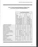 Methods
available laboratory and data analysis methods. The essential elements of appropriate,
method-specific quality assurance and quality control programs and statistical design
considerations are described, and an assessment of how the data generated can be
used in a 403 assessment is provided. All of the information presented for each
monitoring program component is summarized at the end of the section. Numerous
references are also presented in Appendix A to provide the reader with additional
sources of more detailed information concerning the use of the various methods.
This methods chapter is also intended to provide a summary of available information
and to address the most important issues associated with the design and
implementation of the monitoring program. Issues common to all monitoring methods
include quality assurance/quality control (QA/QC) and statistical design.
Quality Assurance/Quality Control Considerations - A QA/QC plan should be
developed to ensure the reliability and compatibility of data collected during the
monitoring program. Quality assurance (QA), implemented at the management level,
focuses on guidelines and procedures, such as delegation of authority and
responsibility, to ensure data quality. Quality control (QC) centers on the technical
activities, such as calibration or interlaboratory studies, needed to achieve specific data
quality. QA is a discipline that begins with effective and conscientious work planning
and ends with a carefully constructed set of checks and balances designed to ensure
that uncertainties have;been reduced to a known practical minimum (USEPA 1987c).
QA is achieved by adopting specific guidelines and procedures to be followed during
sample collection, sample analysis, data handling, and data analysis. These guidelines
and procedures provide program quality control. QC includes the use of blanks and
replicate samples to check field and laboratory sampling and handling techniques and to
examine natural variability in contaminant concentrations. ;
Establishment of data quality standards is fundamental to the selection of monitoring
methods and ensures comparability among data collected. A quality assurance plan
should be developed by each monitoring program to standardize fundamental aspects of
data collection and handling. Although the topics to be considered in a quality
assurance plan will vary somewhat among programs, examples of some key
considerations are provided in Table 4-3.
Data Quality Objectives - A major part of the QA effort is the establishment of Data
Quality Objectives (DQOs). DQOs are specific, integrated statements and goals
developed for each data or information collection activity to ensure that the data are of
the required quantity and quality. DQOs should specify the desired sensitivity of
sampling methods, timing of sampling, and numbers of samples to be collected. One
function of establishing DQOs is to ensure that monitoring/data collection studies yield
data adequate to meet their intended uses. DQOs (or data performance criteria) are
also used to delineate QA/QC programs specifically geared to the data collection
34
image:
Methods
available laboratory and data analysis methods. The essential elements of appropriate,
method-specific quality assurance and quality control programs and statistical design
considerations are described, and an assessment of how the data generated can be
used in a 403 assessment is provided. All of the information presented for each
monitoring program component is summarized at the end of the section. Numerous
references are also presented in Appendix A to provide the reader with additional
sources of more detailed information concerning the use of the various methods.
This methods chapter is also intended to provide a summary of available information
and to address the most important issues associated with the design and
implementation of the monitoring program. Issues common to all monitoring methods
include quality assurance/quality control (QA/QC) and statistical design.
Quality Assurance/Quality Control Considerations - A QA/QC plan should be
developed to ensure the reliability and compatibility of data collected during the
monitoring program. Quality assurance (QA), implemented at the management level,
focuses on guidelines and procedures, such as delegation of authority and
responsibility, to ensure data quality. Quality control (QC) centers on the technical
activities, such as calibration or interlaboratory studies, needed to achieve specific data
quality. QA is a discipline that begins with effective and conscientious work planning
and ends with a carefully constructed set of checks and balances designed to ensure
that uncertainties have;been reduced to a known practical minimum (USEPA 1987c).
QA is achieved by adopting specific guidelines and procedures to be followed during
sample collection, sample analysis, data handling, and data analysis. These guidelines
and procedures provide program quality control. QC includes the use of blanks and
replicate samples to check field and laboratory sampling and handling techniques and to
examine natural variability in contaminant concentrations. ;
Establishment of data quality standards is fundamental to the selection of monitoring
methods and ensures comparability among data collected. A quality assurance plan
should be developed by each monitoring program to standardize fundamental aspects of
data collection and handling. Although the topics to be considered in a quality
assurance plan will vary somewhat among programs, examples of some key
considerations are provided in Table 4-3.
Data Quality Objectives - A major part of the QA effort is the establishment of Data
Quality Objectives (DQOs). DQOs are specific, integrated statements and goals
developed for each data or information collection activity to ensure that the data are of
the required quantity and quality. DQOs should specify the desired sensitivity of
sampling methods, timing of sampling, and numbers of samples to be collected. One
function of establishing DQOs is to ensure that monitoring/data collection studies yield
data adequate to meet their intended uses. DQOs (or data performance criteria) are
also used to delineate QA/QC programs specifically geared to the data collection
34
image:
 Section 403 Procedural and Monitoring Guidance
Table 4-3. Key Topics to Be Addressed in Marine Monitoring
Program Quality Assurance Plans
• Instructions for proper sample preservation and storage
• Chain of custody documentation
• Source of standard reagents
• Source or preparation of quality control samples
• Frequency of analysis of quality control samples
• Data Quality Objectives
• Analysis of QC samples
• Review of results
• Corrective action when unsatisfactory results are obtained in the
analysis of QA/QC samples
• Calibration and maintenance of equipment
activities to be undertaken. Development of DQOs usually consists of three processes:
(1) decision definition, (2) data use and needs identification, and (3) data collection
program design. DQOs should be continually reviewed during data collection activities
so that any needed corrective action may be planned and executed to minimize
problems before they become significant.
DQOs play an important role in the selection of sample collection, sorting, and analysis
methods. In fact, the selection of monitoring methods should be driven by DQOs. Any
future modifications to monitoring protocols should be considered only after these new
methods meet established data performance criteria. Data collected using different
methods should not be compared unless information exists that supports such
comparisons.
35
image:
Section 403 Procedural and Monitoring Guidance
Table 4-3. Key Topics to Be Addressed in Marine Monitoring
Program Quality Assurance Plans
• Instructions for proper sample preservation and storage
• Chain of custody documentation
• Source of standard reagents
• Source or preparation of quality control samples
• Frequency of analysis of quality control samples
• Data Quality Objectives
• Analysis of QC samples
• Review of results
• Corrective action when unsatisfactory results are obtained in the
analysis of QA/QC samples
• Calibration and maintenance of equipment
activities to be undertaken. Development of DQOs usually consists of three processes:
(1) decision definition, (2) data use and needs identification, and (3) data collection
program design. DQOs should be continually reviewed during data collection activities
so that any needed corrective action may be planned and executed to minimize
problems before they become significant.
DQOs play an important role in the selection of sample collection, sorting, and analysis
methods. In fact, the selection of monitoring methods should be driven by DQOs. Any
future modifications to monitoring protocols should be considered only after these new
methods meet established data performance criteria. Data collected using different
methods should not be compared unless information exists that supports such
comparisons.
35
image:
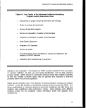 Methods
The methods sections that follow provide a discussion of existing monitoring methods.
These methods provide a starting point for considering monitoring methodologies. New,
cost-effective methods are sure to be developed for certain disciplines in the coming
years. A key consideration when determining whether new methods are to be
incorporated into the monitoring program is whether they meet the performance criteria
of the QA/QC program. QA/QC considerations in the methods sections focus primarily
on sample collection, processing, storage, and analysis.
QC Samples - Additional samples, either collected in the field or prepared from
standard reference materials, are used to check for field or laboratory contamination,
test laboratory accuracy, test field or laboratory reproducibility, and assess natural
variability. Four basic types of QC samples should be submitted with each set of
sediment or water quality samples (Table 4-4). Although the frequency with which these
samples are collected will vary among programs, each should be collected at least once
for every 20 samples or sampling event, whichever is more frequent.
Data from other existing monitoring programs will often be used in a monitoring
program. Therefore, data will frequently be collected by a number of agencies following
different sampling and analytical strategies. Under such conditions data comparability
becomes a major QA/QC consideration. Data comparability must be evaluated based
on both field and laboratory sources of variability. Individual programs will need to
address this aspect of QA on a case-by-case basis.
Table 4-4. QC Sample Types
Travel (trip) Blank
Rinsate Blank
Method Blank
Field Split
Assess cross-contamination during handling
and transport
Assess contamination due to incomplete
cleaning of sample equipment
Assess sample contamination due to
reagents/sample handling in the laboratory
Assess variability in sampling technique and/or
laboratory handling
36
image:
Methods
The methods sections that follow provide a discussion of existing monitoring methods.
These methods provide a starting point for considering monitoring methodologies. New,
cost-effective methods are sure to be developed for certain disciplines in the coming
years. A key consideration when determining whether new methods are to be
incorporated into the monitoring program is whether they meet the performance criteria
of the QA/QC program. QA/QC considerations in the methods sections focus primarily
on sample collection, processing, storage, and analysis.
QC Samples - Additional samples, either collected in the field or prepared from
standard reference materials, are used to check for field or laboratory contamination,
test laboratory accuracy, test field or laboratory reproducibility, and assess natural
variability. Four basic types of QC samples should be submitted with each set of
sediment or water quality samples (Table 4-4). Although the frequency with which these
samples are collected will vary among programs, each should be collected at least once
for every 20 samples or sampling event, whichever is more frequent.
Data from other existing monitoring programs will often be used in a monitoring
program. Therefore, data will frequently be collected by a number of agencies following
different sampling and analytical strategies. Under such conditions data comparability
becomes a major QA/QC consideration. Data comparability must be evaluated based
on both field and laboratory sources of variability. Individual programs will need to
address this aspect of QA on a case-by-case basis.
Table 4-4. QC Sample Types
Travel (trip) Blank
Rinsate Blank
Method Blank
Field Split
Assess cross-contamination during handling
and transport
Assess contamination due to incomplete
cleaning of sample equipment
Assess sample contamination due to
reagents/sample handling in the laboratory
Assess variability in sampling technique and/or
laboratory handling
36
image:
 Section 403 Procedural and Mon/foring Guidance
Statistical Design Considerations - Prior to the collection of data, how the data will be
used to generate pertinent information essential to making sound decisions should be
specified. It is further recommended that analytical performance criteria (e.g., minimally
acceptable Type I and Type II error) be defined to establish quantitative expectations for
the monitoring program. The link between data, performance, and decision-making
should be specified a priori to ensure that appropriate data are obtained and that spatial
and temporal variations are addressed by the monitoring plan.
Selection of the number of replicates is an important component of program design.
The use of power analyses, examining alternative sampling and compositing strategies,
will lead to an effective monitoring design strategy. These statistical techniques may
mitigate the high costs of collecting and processing samples. As a general
recommendation, samples of equal size should be collected whenever possible to
simplify statistical analyses.
Composite Sampling - Composite sampling consists of mixing two or more replicates
and/or samples. The chemical analysis of a composite sample provides an estimate of
an average contaminant concentration for locations and/or times composing the
composite sample (see space and time bulking below). Advantages of the composite
sampling strategy are that it provides a cost-effective strategy when individual chemical
analyses are expensive and it results in a more efficient estimate of the mean at
specified sampling locations.
Because of the reduced sample variance, composite sampling may result in a
considerable increase in statistical power. If the primary objective of a monitoring
program is to determine differences in contaminant concentrations among sampling
locations, composite sampling is an appropriate strategy.
Space-bulking consists of sampling from several locations and combining samples into
one or more composite samples. Time-bulking involves taking multiple samples over
time from a single location and compositing these samples. The use of space- and/or
time-bulking strategies should be considered with the awareness that significant
information concerning spatial and temporal heterogeneity may be lost.
Compositing of tissues provides a means to analyze bioaccumulation when the tissue
mass of an individual is insufficient for the analytical protocol.- If mixing species, tissue
composites are likely to be composed of different proportions of species and different
numbers, ages, and sexes of individuals. These differences among composites tend to
confound the question of whether patterns of tissue residue concentrations are due to
differences in locations or interspecific differences in bioaccumulation. Mixing of species
is not recommended because of these confounding effects.
37
image:
Section 403 Procedural and Mon/foring Guidance
Statistical Design Considerations - Prior to the collection of data, how the data will be
used to generate pertinent information essential to making sound decisions should be
specified. It is further recommended that analytical performance criteria (e.g., minimally
acceptable Type I and Type II error) be defined to establish quantitative expectations for
the monitoring program. The link between data, performance, and decision-making
should be specified a priori to ensure that appropriate data are obtained and that spatial
and temporal variations are addressed by the monitoring plan.
Selection of the number of replicates is an important component of program design.
The use of power analyses, examining alternative sampling and compositing strategies,
will lead to an effective monitoring design strategy. These statistical techniques may
mitigate the high costs of collecting and processing samples. As a general
recommendation, samples of equal size should be collected whenever possible to
simplify statistical analyses.
Composite Sampling - Composite sampling consists of mixing two or more replicates
and/or samples. The chemical analysis of a composite sample provides an estimate of
an average contaminant concentration for locations and/or times composing the
composite sample (see space and time bulking below). Advantages of the composite
sampling strategy are that it provides a cost-effective strategy when individual chemical
analyses are expensive and it results in a more efficient estimate of the mean at
specified sampling locations.
Because of the reduced sample variance, composite sampling may result in a
considerable increase in statistical power. If the primary objective of a monitoring
program is to determine differences in contaminant concentrations among sampling
locations, composite sampling is an appropriate strategy.
Space-bulking consists of sampling from several locations and combining samples into
one or more composite samples. Time-bulking involves taking multiple samples over
time from a single location and compositing these samples. The use of space- and/or
time-bulking strategies should be considered with the awareness that significant
information concerning spatial and temporal heterogeneity may be lost.
Compositing of tissues provides a means to analyze bioaccumulation when the tissue
mass of an individual is insufficient for the analytical protocol.- If mixing species, tissue
composites are likely to be composed of different proportions of species and different
numbers, ages, and sexes of individuals. These differences among composites tend to
confound the question of whether patterns of tissue residue concentrations are due to
differences in locations or interspecific differences in bioaccumulation. Mixing of species
is not recommended because of these confounding effects.
37
image:
 Methods
Composite sampling is not recommended if the objective of the monitoring program is to
determine compliance with specified sediment contaminant concentration limits since
this sampling method does not detect the true range of sediment contaminant
concentrations in the environment. The adoption of composite strategies will depend on
the objectives of individual monitoring programs.
Statistical Power - The large degree of temporal and spatial variability observed for
many ecosystem state and rate variables requires collection of sufficient replicate
samples to ensure an accurate description of the measure of interest. However,
increases in replication increase sample processing costs. Power analyses assist in the
allocation of sampling resources (stations, replication, and frequency) with regard to
program finances and design (Sokal and Rohlf, 1981).
Power analyses may be applied to determine the appropriate number of sample
replicates and/or subsamples in a replicate composite required to detect a specified
difference (USEPA, 1987d). Statistical power increases with the increase of sample
replicates. However, there is a point of diminishing return of statistical power with the
addition of successive sample replicates (USEPA, 1987d). The number of replications
required to detect a specified minimum difference is a function of the statistical power
and the variance in the data. Power analyses require a priori knowledge of the
variability in the data. A best guess or, preferably, variation observed in historical data is
often used initially in the design of the monitoring program.
For composite samples, statistical power increases with an increase in the number of
subsamples in each replicate composite sample (USEPA, 1987a); however, with the
addition of successive subsamples to each composite, a diminished return of statistical
power exists. For composites of greater than 10 replications, the increase of power is
negligible given typical levels of data variability.
To improve the power of a statistical test while keeping the significant level constant, the
sample size should be increased; however, because of constraints in cost and time, this
option may not be available. Power analyses have shown that, for a fixed level of
sampling effort, a monitoring program's power is generally increased by collecting more
replicates at fewer locations. The number and distribution of sampling locations
required to evaluate the effectiveness of the monitoring program will depend on the size
and complexity of the site under investigation.
Power-Cost Analyses - The relative power of one design with respect to another is
more meaningful when the relative costs of implementing alternative designs are taken
into consideration. Power-cost analyses are fundamental in selecting appropriate
sample/replicate number, sample location, and sampling frequency (Bros and Cowell,
1987; Cuff and Coleman, 1979; Ferraro etal., 1989; Millard and Lettenmaier, 1986).
38
image:
Methods
Composite sampling is not recommended if the objective of the monitoring program is to
determine compliance with specified sediment contaminant concentration limits since
this sampling method does not detect the true range of sediment contaminant
concentrations in the environment. The adoption of composite strategies will depend on
the objectives of individual monitoring programs.
Statistical Power - The large degree of temporal and spatial variability observed for
many ecosystem state and rate variables requires collection of sufficient replicate
samples to ensure an accurate description of the measure of interest. However,
increases in replication increase sample processing costs. Power analyses assist in the
allocation of sampling resources (stations, replication, and frequency) with regard to
program finances and design (Sokal and Rohlf, 1981).
Power analyses may be applied to determine the appropriate number of sample
replicates and/or subsamples in a replicate composite required to detect a specified
difference (USEPA, 1987d). Statistical power increases with the increase of sample
replicates. However, there is a point of diminishing return of statistical power with the
addition of successive sample replicates (USEPA, 1987d). The number of replications
required to detect a specified minimum difference is a function of the statistical power
and the variance in the data. Power analyses require a priori knowledge of the
variability in the data. A best guess or, preferably, variation observed in historical data is
often used initially in the design of the monitoring program.
For composite samples, statistical power increases with an increase in the number of
subsamples in each replicate composite sample (USEPA, 1987a); however, with the
addition of successive subsamples to each composite, a diminished return of statistical
power exists. For composites of greater than 10 replications, the increase of power is
negligible given typical levels of data variability.
To improve the power of a statistical test while keeping the significant level constant, the
sample size should be increased; however, because of constraints in cost and time, this
option may not be available. Power analyses have shown that, for a fixed level of
sampling effort, a monitoring program's power is generally increased by collecting more
replicates at fewer locations. The number and distribution of sampling locations
required to evaluate the effectiveness of the monitoring program will depend on the size
and complexity of the site under investigation.
Power-Cost Analyses - The relative power of one design with respect to another is
more meaningful when the relative costs of implementing alternative designs are taken
into consideration. Power-cost analyses are fundamental in selecting appropriate
sample/replicate number, sample location, and sampling frequency (Bros and Cowell,
1987; Cuff and Coleman, 1979; Ferraro etal., 1989; Millard and Lettenmaier, 1986).
38
image:
 Section 403 Procedural and Monitoring Guidance
A cost function that describes the cost per replicate sample is required. Power-cost
formulations for parametric statistical analyses are of the form:
Power-cost j = (1 - p j) / (Ci x ni)
where i is a replicate sample collection and analysis scheme, c is the cost per replicate
sample, n is the number of replicate samples, and p is the Type II error. Costs will
depend on sample collection, sorting, analysis equipment, and protocols. Type II error
(p) is a function of the number of replicate samples and the variance detected by a
sampling and analysis scheme. The measured variance may be influenced by the
sampling equipment used and the unit replicate sample size (e.g., as the unit replicate
area approaches patch size, variance increases).
Since total costs are usually fixed, iterations of power-cost formulations for various
sample processing scenarios (e.g., sample collection, sorting, and analysis schemes)
and their comparisons will result in the selection of the appropriate monitoring
methodology. Sokal and Rohlf (1981) provide a series of formulas for calculating the
most efficient sampling design for a given cost.
39
image:
Section 403 Procedural and Monitoring Guidance
A cost function that describes the cost per replicate sample is required. Power-cost
formulations for parametric statistical analyses are of the form:
Power-cost j = (1 - p j) / (Ci x ni)
where i is a replicate sample collection and analysis scheme, c is the cost per replicate
sample, n is the number of replicate samples, and p is the Type II error. Costs will
depend on sample collection, sorting, analysis equipment, and protocols. Type II error
(p) is a function of the number of replicate samples and the variance detected by a
sampling and analysis scheme. The measured variance may be influenced by the
sampling equipment used and the unit replicate sample size (e.g., as the unit replicate
area approaches patch size, variance increases).
Since total costs are usually fixed, iterations of power-cost formulations for various
sample processing scenarios (e.g., sample collection, sorting, and analysis schemes)
and their comparisons will result in the selection of the appropriate monitoring
methodology. Sokal and Rohlf (1981) provide a series of formulas for calculating the
most efficient sampling design for a given cost.
39
image:
 Methods
4.1 PHYSICAL CHARACTERISTICS
Physical characteristics are typically measured in situ and include temperature, salinity,
density, depth, turbidity, and current velocity and direction. Physical data are used to
characterize the water column, verify hydrodynamic models, and indicate spatial and
temporal variations.
4.1.1
Rationale
Of the 10 guidelines used to determine unreasonable degradation or irreparable harm,
the following can be assessed by evaluating physical characteristics:
. Potential transport of the pollutants by biological, physical, or chemical
processes and
• Marine water quality criteria.
Most chemical and biological processes in the marine environment are affected, either
directly or indirectly, by physical characteristics of the marine environment (Thomann
and Mueller, 1987). Consequently, physical characteristics are used to determine plume
and sediment movement (hydrodynamics and fate and transport modeling) and to
provide ancillary information to interpret other water chemistry variables. In addition, to
ensure protection of the characteristic indigenous marine community, national
temperature criteria have been established in the "Gold Book" (USEEPA, 1986d).
All biological monitoring should include consistent physical habitat variable
measurements and physical habitat matches between sampling sites and reference
sites or identified conditions in order to accurately assess the condition of biological
resources in the area of sampling. Physical measurement data such as grain size,
depth, salinity, temperature, dissolved oxygen, and vegetative cover should be
measured along with biological variable measurements.
4.1.2 Monitoring Design Considerations
The main uses of physical data are to characterize the area in the vicinity of the
discharge site and to serve as ancillary information for other variables. As a result,
temperature, salinity, density, turbidity, and depth (depth of sample and depth to bottom)
should be collected at every station location. The cost of the various methods is
controlled by the level of automation and, in comparison, physical data collection is
relatively inexpensive. In many instances, the sampling location and frequency will be
controlled by other more expensively collected variables. The number and location of
current measurements should be based on the complexity of the circulation patterns and
effluent characteristics.
40
image:
Methods
4.1 PHYSICAL CHARACTERISTICS
Physical characteristics are typically measured in situ and include temperature, salinity,
density, depth, turbidity, and current velocity and direction. Physical data are used to
characterize the water column, verify hydrodynamic models, and indicate spatial and
temporal variations.
4.1.1
Rationale
Of the 10 guidelines used to determine unreasonable degradation or irreparable harm,
the following can be assessed by evaluating physical characteristics:
. Potential transport of the pollutants by biological, physical, or chemical
processes and
• Marine water quality criteria.
Most chemical and biological processes in the marine environment are affected, either
directly or indirectly, by physical characteristics of the marine environment (Thomann
and Mueller, 1987). Consequently, physical characteristics are used to determine plume
and sediment movement (hydrodynamics and fate and transport modeling) and to
provide ancillary information to interpret other water chemistry variables. In addition, to
ensure protection of the characteristic indigenous marine community, national
temperature criteria have been established in the "Gold Book" (USEEPA, 1986d).
All biological monitoring should include consistent physical habitat variable
measurements and physical habitat matches between sampling sites and reference
sites or identified conditions in order to accurately assess the condition of biological
resources in the area of sampling. Physical measurement data such as grain size,
depth, salinity, temperature, dissolved oxygen, and vegetative cover should be
measured along with biological variable measurements.
4.1.2 Monitoring Design Considerations
The main uses of physical data are to characterize the area in the vicinity of the
discharge site and to serve as ancillary information for other variables. As a result,
temperature, salinity, density, turbidity, and depth (depth of sample and depth to bottom)
should be collected at every station location. The cost of the various methods is
controlled by the level of automation and, in comparison, physical data collection is
relatively inexpensive. In many instances, the sampling location and frequency will be
controlled by other more expensively collected variables. The number and location of
current measurements should be based on the complexity of the circulation patterns and
effluent characteristics.
40
image:
 Section 403 Procedural and Monitoring Guidance
If a mathematical model will be used to assess the effects of ambient physical
characteristics and the fate and transport of the discharged effluent, the monitoring
program should be designed to provide the model with the required forcing boundary
condition data. It may also be necessary to collect meteorological data (e.g., wind
speed and direction, temperature, pressure) for modeling efforts since plumes can be
affected by wind effects.
General recommendations for sampling locations include the following:
• To predict potential transport of the pollutants by biological, physical, or
chemical processes, sampling stations need to be located in the vicinity of the
zone of initial dilution (ZID) boundary, at control sites, and in impacted areas
to allow adequate correlations to be made between water quality,
oceanographic measurements, toxic substances, and biological data
(USEPA, 1982a). Other locations may include the shoreline in swimming and
shellfishery areas and within the ZID (Koh, 1988).
• Additional monitoring stations should be located near other pollutant sources,
as applicable, to allow the effects of the subject discharge to be distinguished
from these sources.
• Several samples should be taken at various depths across the waste field as
the plume crosses the ZID boundary.
• Sampling depths are generally acceptable if taken at standard depths (Pond
and Pickard, 1983); however, features of water masses observed in profiling
for salinity, temperature, and turbidity should take precedence in establishing
sample depths. When using in situ methods (e.g., CTD), temperature and
salinity measurements should be taken at 1-meter intervals over the entire
depth profile (to within 1 meter of the surface and bottom). In areas of high
stratification, a smaller interval would be appropriate.
• As a practical minimum when using bottle sampling techniques, samples for
temperature, salinity, and turbidity should be taken at four depths in the
vertical profile: (1) 1 meter below the surface, (2) 1 meter above the bottom,
(3) 1 meter above the pycnocline, and (4) 1 meter below the pycnocline. If
the waters are too shallow or no stratification occurs, it would be appropriate
to take the latter two samples at evenly spaced distances between the top
and bottom samples. In many cases, these depths will coincide with
variables described in other sections.
General recommendations for sampling frequency include the following:
• Sampling frequency should be high enough to differentiate between
high-frequency natural events (e.g., tides, storms) and mean conditions.
41
image:
Section 403 Procedural and Monitoring Guidance
If a mathematical model will be used to assess the effects of ambient physical
characteristics and the fate and transport of the discharged effluent, the monitoring
program should be designed to provide the model with the required forcing boundary
condition data. It may also be necessary to collect meteorological data (e.g., wind
speed and direction, temperature, pressure) for modeling efforts since plumes can be
affected by wind effects.
General recommendations for sampling locations include the following:
• To predict potential transport of the pollutants by biological, physical, or
chemical processes, sampling stations need to be located in the vicinity of the
zone of initial dilution (ZID) boundary, at control sites, and in impacted areas
to allow adequate correlations to be made between water quality,
oceanographic measurements, toxic substances, and biological data
(USEPA, 1982a). Other locations may include the shoreline in swimming and
shellfishery areas and within the ZID (Koh, 1988).
• Additional monitoring stations should be located near other pollutant sources,
as applicable, to allow the effects of the subject discharge to be distinguished
from these sources.
• Several samples should be taken at various depths across the waste field as
the plume crosses the ZID boundary.
• Sampling depths are generally acceptable if taken at standard depths (Pond
and Pickard, 1983); however, features of water masses observed in profiling
for salinity, temperature, and turbidity should take precedence in establishing
sample depths. When using in situ methods (e.g., CTD), temperature and
salinity measurements should be taken at 1-meter intervals over the entire
depth profile (to within 1 meter of the surface and bottom). In areas of high
stratification, a smaller interval would be appropriate.
• As a practical minimum when using bottle sampling techniques, samples for
temperature, salinity, and turbidity should be taken at four depths in the
vertical profile: (1) 1 meter below the surface, (2) 1 meter above the bottom,
(3) 1 meter above the pycnocline, and (4) 1 meter below the pycnocline. If
the waters are too shallow or no stratification occurs, it would be appropriate
to take the latter two samples at evenly spaced distances between the top
and bottom samples. In many cases, these depths will coincide with
variables described in other sections.
General recommendations for sampling frequency include the following:
• Sampling frequency should be high enough to differentiate between
high-frequency natural events (e.g., tides, storms) and mean conditions.
41
image:
 Methods
• To establish meaningful estimates of the plume behavior, it is essential that
the monitoring program encompass the range of conditions that might occur.
In particular, to obtain seasonal variations, measurements should extend for
at least 2 years.
• Sampling frequency of temperature and salinity should be selected to provide
data for critical periods (e.g., time of seasonal maximum and minimum
stratification, low net circulation, time and duration of coastal upwelling, and
exceptional biological activity).
• In monitoring the other physical characteristics of the receiving water,
sampling events and frequencies should be timed to provide information
during critical environmental periods.
• More frequent sampling in fish and shellfish harvesting areas, and in other
biologically sensitive areas, may be required.
Moored instrument arrays provide a cost-effective method of continual sampling over
long periods of time (from days to months) for many physical characteristics. More
commonly used at remote offshore locations, subsurface arrays can provide unattended
long-term data collection in estuarine environments for both physical and chemical
parameters. Water depth, velocity (speed and direction), temperature, and conductivity
or salinity are the most commonly measured characteristics. Estimates of total
suspended solids and chlorophyll can be recorded also, using turbidometers,
transmissometers, or fluorometers. Dissolved oxygen concentrations can also be
measured. Sensors capable of in situ measurements of nutrient and trace contaminant
concentrations are under development.
Moored arrays have the potential to provide synoptic coverage at predetermined
intervals, which can range from minutes to days. The longer the interval between data
recordings, the longer the array can function without replacing the power supply (usually
batteries) or the recording medium (cassette tape or computer memory chips).
Real-time telemetry of data to a shore station is possible with the more sophisticated
(and more expensive) instrumentation packages. More commonly, the instrument array
is retrieved at regular intervals and the collected data post-processed. Moored arrays
that are deployed for long periods of time are susceptible to many types of interference.
4.1.3 Analytical Methods Considerations
Methods available for measuring physical characteristics include instruments that range
from simple mercury-filled thermometers that provide one observation of temperature to
state-of-the-art CTD (conductivity-temperature-depth) meters that provide vertical
profiles of salinity and temperature. Methods and/or equipment discussed in this section
are listed in Table 4-5.
42
image:
Methods
• To establish meaningful estimates of the plume behavior, it is essential that
the monitoring program encompass the range of conditions that might occur.
In particular, to obtain seasonal variations, measurements should extend for
at least 2 years.
• Sampling frequency of temperature and salinity should be selected to provide
data for critical periods (e.g., time of seasonal maximum and minimum
stratification, low net circulation, time and duration of coastal upwelling, and
exceptional biological activity).
• In monitoring the other physical characteristics of the receiving water,
sampling events and frequencies should be timed to provide information
during critical environmental periods.
• More frequent sampling in fish and shellfish harvesting areas, and in other
biologically sensitive areas, may be required.
Moored instrument arrays provide a cost-effective method of continual sampling over
long periods of time (from days to months) for many physical characteristics. More
commonly used at remote offshore locations, subsurface arrays can provide unattended
long-term data collection in estuarine environments for both physical and chemical
parameters. Water depth, velocity (speed and direction), temperature, and conductivity
or salinity are the most commonly measured characteristics. Estimates of total
suspended solids and chlorophyll can be recorded also, using turbidometers,
transmissometers, or fluorometers. Dissolved oxygen concentrations can also be
measured. Sensors capable of in situ measurements of nutrient and trace contaminant
concentrations are under development.
Moored arrays have the potential to provide synoptic coverage at predetermined
intervals, which can range from minutes to days. The longer the interval between data
recordings, the longer the array can function without replacing the power supply (usually
batteries) or the recording medium (cassette tape or computer memory chips).
Real-time telemetry of data to a shore station is possible with the more sophisticated
(and more expensive) instrumentation packages. More commonly, the instrument array
is retrieved at regular intervals and the collected data post-processed. Moored arrays
that are deployed for long periods of time are susceptible to many types of interference.
4.1.3 Analytical Methods Considerations
Methods available for measuring physical characteristics include instruments that range
from simple mercury-filled thermometers that provide one observation of temperature to
state-of-the-art CTD (conductivity-temperature-depth) meters that provide vertical
profiles of salinity and temperature. Methods and/or equipment discussed in this section
are listed in Table 4-5.
42
image:
 Section 403 Procedural ancf Monitoring Guidance
Table 4-5. List of Methods and Equipment
Temperature
Turbidity
Salinity
Density
Depth
mercury-filled or dial-type
centigrade thermometer
thermistor
reverse thermometer
bathythermograph
CTD
Knudsen titration
conductivity cells (CTD instruments)
direct (hydrometers, pycnometers,
magnetic float densimeters)
indirect (function of salinity,
temperature, and pressure)
fathometer
meter wheel
hydrostatic pressure
bourdon tube
strain gauge
light transmissometer
Secchi disc
nephelometer
turbidimeter
Current Measurements
Eulerian Method (speed and
direction)
mechanical
electromagnetic
acoustic
Lagrangian Method
drogues
surface drifters
seabed drifters
Dye Studies
fluorometer
43
image:
Section 403 Procedural ancf Monitoring Guidance
Table 4-5. List of Methods and Equipment
Temperature
Turbidity
Salinity
Density
Depth
mercury-filled or dial-type
centigrade thermometer
thermistor
reverse thermometer
bathythermograph
CTD
Knudsen titration
conductivity cells (CTD instruments)
direct (hydrometers, pycnometers,
magnetic float densimeters)
indirect (function of salinity,
temperature, and pressure)
fathometer
meter wheel
hydrostatic pressure
bourdon tube
strain gauge
light transmissometer
Secchi disc
nephelometer
turbidimeter
Current Measurements
Eulerian Method (speed and
direction)
mechanical
electromagnetic
acoustic
Lagrangian Method
drogues
surface drifters
seabed drifters
Dye Studies
fluorometer
43
image:
 Methods
Temperature
Temperature measurements may be made with any good grade of mercury-filled or
dial-type centigrade thermometer, or a thermistor (USEPA, 1983a, Standard Method
170.1). Surface temperatures (from bucket samples) may be taken using an ordinary
mercury thermometer, taking care not to expose the bucket to the sun (heating) or to the
evaporating influence of the wind (cooling).
For measuring subsurface temperatures, the basic instrument is the "protected reversing
thermometer," a mercury-in-glass thermometer that is attached to the water sampling
bottle. When the sample bottle is closed, the thermometer is inverted. The mercury
"breaks" at a particular point and runs to the other end of the capillary, thereby recording
the temperature of the water at the depth where the sample was taken (UNESCO,
1988).
A bathythermograph (BT) consists of a thermistor and an electronic pressure
transducer. Wire extending from the BT to the vessel relays measures of temperature
and pressure. BTs may be operated from stationary or slow-moving (<4 knots) vessels.
Expendable bathythermographs (XBTs) are based on tracking an expendable,
free-fa||jng temperature sensor. The system is designed to operate from a stationary or
moving vessel (<15 to 20 knots) typically in deep waters. Wires extending from the
free-falling transducer to the vessel relay temperature and depth recordings. The wires
are cut when the probe reaches its maximum depth. BTs and XBTs do not record
measures of salinity. If it has been determined that density is not related to salinity,
bathythermographs may be a cost-effective tool. Monitoring of temperature and
pressure using XBTs is higher in cost since the probe is lost after each vertical profile.
Conductivity-temperature-depth meters (CTDs) are the tool of choice since density
measures are typically dependent on salinity, temperature, and depth (see Density
below). Measures of density are important in identifying and tracking the movements of
waterbodies and in determining the depth at which a water mass will settle at
equilibrium. CTDs coupled with a computer can continuously integrate temperature and
conductivity measurements with depth. The CTD/computer combination provides
real-time readouts that allow immediate modifications in CTD position and ensures
comprehensive water column coverage during the survey.
Salinity
The Knudsen titration method determines chlorinity by titration with a standard silver
nitrate solution, and salinity is then computed from a standard formula (Pond and
Pickard, 1983). This titration method is practical but not convenient to use on board a
ship (APHA, 1989).
44
image:
Methods
Temperature
Temperature measurements may be made with any good grade of mercury-filled or
dial-type centigrade thermometer, or a thermistor (USEPA, 1983a, Standard Method
170.1). Surface temperatures (from bucket samples) may be taken using an ordinary
mercury thermometer, taking care not to expose the bucket to the sun (heating) or to the
evaporating influence of the wind (cooling).
For measuring subsurface temperatures, the basic instrument is the "protected reversing
thermometer," a mercury-in-glass thermometer that is attached to the water sampling
bottle. When the sample bottle is closed, the thermometer is inverted. The mercury
"breaks" at a particular point and runs to the other end of the capillary, thereby recording
the temperature of the water at the depth where the sample was taken (UNESCO,
1988).
A bathythermograph (BT) consists of a thermistor and an electronic pressure
transducer. Wire extending from the BT to the vessel relays measures of temperature
and pressure. BTs may be operated from stationary or slow-moving (<4 knots) vessels.
Expendable bathythermographs (XBTs) are based on tracking an expendable,
free-fa||jng temperature sensor. The system is designed to operate from a stationary or
moving vessel (<15 to 20 knots) typically in deep waters. Wires extending from the
free-falling transducer to the vessel relay temperature and depth recordings. The wires
are cut when the probe reaches its maximum depth. BTs and XBTs do not record
measures of salinity. If it has been determined that density is not related to salinity,
bathythermographs may be a cost-effective tool. Monitoring of temperature and
pressure using XBTs is higher in cost since the probe is lost after each vertical profile.
Conductivity-temperature-depth meters (CTDs) are the tool of choice since density
measures are typically dependent on salinity, temperature, and depth (see Density
below). Measures of density are important in identifying and tracking the movements of
waterbodies and in determining the depth at which a water mass will settle at
equilibrium. CTDs coupled with a computer can continuously integrate temperature and
conductivity measurements with depth. The CTD/computer combination provides
real-time readouts that allow immediate modifications in CTD position and ensures
comprehensive water column coverage during the survey.
Salinity
The Knudsen titration method determines chlorinity by titration with a standard silver
nitrate solution, and salinity is then computed from a standard formula (Pond and
Pickard, 1983). This titration method is practical but not convenient to use on board a
ship (APHA, 1989).
44
image:
 Section 403 Procedural and Monitoring Guidance
Conductive cells are used for in situ measurements, and a variety of such instruments
are now available from several manufacturers (Pond and Pickard, 1983). A CTD unit
consisting of conductivity, temperature, and depth sensors is lowered through the water
on the end of an electrical conductor cable, which transmits the information to recording
units on board ship (UNESCO, 1988).
Density
Direct measurement of density is generally not accurate enough for most oceanographic
considerations (Pond and Pickard, 1983). Nevertheless, devices such as hydrometers,
pycnometers, and magnetic float densimeters are sometimes used when great accuracy
is not required.
In the absence of adequate means to measure seawater density accurately and quickly,
it is common practice to determine density indirectly from salinity, temperature, and
pressure. The density (or the specific gravity) of seawater depends on the temperature,
salinity, and (as a result of the slight compressibility of water) pressure. In practice,
temperature, salinity, and pressure are measured and the density is read from tables
that have been prepared from laboratory determinations (e.g., Eugene, 1966).
Algorithms for automated data processing have been developed by UNESCO and are
applicable for salinities as low as 2 ppt (Fofonoff and Millard, 1983). For lower salinities,
see Hill etal. (1986).
The simplest method to determine depth is to pass the wire that is attached to the
instrument over a meter wheel with a known circumference and a counter. In calm
conditions and negligible currents, the length of wire used will be the actual depth.
Depth may also be estimated using a bourdon tube. The tube moves either the slider of
an electrical potentiometer or a strain-gauge pressure transducer, and the resulting
current corresponds to the depth of the instrument.
The total water depth at a particular station is typically determined with acoustic
transponders, which are widely available, are relatively inexpensive, and are accurate to
within 0.3 to 0.7 foot (Clausner et al., 1986).
Turbidity
To determine the transmission of visible light through the water, the simplest device is
the Secchi disc, a black-and-white plate about 30 cm in diameter. The Secchi disc is
lowered into the sea, and the depth at which it is lost to sight is recorded (Pond and
Pickard, 1983). Measurements of Secchi disc depth are probably the most widely used
means of estimating light penetration, and they can be used to estimate the attenuation
45
image:
Section 403 Procedural and Monitoring Guidance
Conductive cells are used for in situ measurements, and a variety of such instruments
are now available from several manufacturers (Pond and Pickard, 1983). A CTD unit
consisting of conductivity, temperature, and depth sensors is lowered through the water
on the end of an electrical conductor cable, which transmits the information to recording
units on board ship (UNESCO, 1988).
Density
Direct measurement of density is generally not accurate enough for most oceanographic
considerations (Pond and Pickard, 1983). Nevertheless, devices such as hydrometers,
pycnometers, and magnetic float densimeters are sometimes used when great accuracy
is not required.
In the absence of adequate means to measure seawater density accurately and quickly,
it is common practice to determine density indirectly from salinity, temperature, and
pressure. The density (or the specific gravity) of seawater depends on the temperature,
salinity, and (as a result of the slight compressibility of water) pressure. In practice,
temperature, salinity, and pressure are measured and the density is read from tables
that have been prepared from laboratory determinations (e.g., Eugene, 1966).
Algorithms for automated data processing have been developed by UNESCO and are
applicable for salinities as low as 2 ppt (Fofonoff and Millard, 1983). For lower salinities,
see Hill etal. (1986).
The simplest method to determine depth is to pass the wire that is attached to the
instrument over a meter wheel with a known circumference and a counter. In calm
conditions and negligible currents, the length of wire used will be the actual depth.
Depth may also be estimated using a bourdon tube. The tube moves either the slider of
an electrical potentiometer or a strain-gauge pressure transducer, and the resulting
current corresponds to the depth of the instrument.
The total water depth at a particular station is typically determined with acoustic
transponders, which are widely available, are relatively inexpensive, and are accurate to
within 0.3 to 0.7 foot (Clausner et al., 1986).
Turbidity
To determine the transmission of visible light through the water, the simplest device is
the Secchi disc, a black-and-white plate about 30 cm in diameter. The Secchi disc is
lowered into the sea, and the depth at which it is lost to sight is recorded (Pond and
Pickard, 1983). Measurements of Secchi disc depth are probably the most widely used
means of estimating light penetration, and they can be used to estimate the attenuation
45
image:
 Methods
coefficients for collimated and diffuse light. As a result, the depth of the euphotic zone
may be estimated. Secchi disc readings vary with the observer because of
interpersonal differences in visual ability; therefore, caution must be exercised when
comparing Secchi disc readings taken by a variety of observers.
Turbidity is the measure of particulate matter (plankton and suspended sediments) in
the water column. Measurements, either in situ or remote, are made by
spectrophotometric methods. This involves passing a light of known intensity and
wavelength through a water sample of precise length. The amount of light received by a
receptor is the percentage of light that has not been absorbed or reflected within the
path length. In remote measurements, water samples are obtained from discrete depths
and then analyzed on deck. This method of sampling is quick and accurate, but it is
labor-intensive and is restricted to sampling only at those depths where water samples
were taken. In situ sampling involves passing a light transmissometer (usually as part of
a CTD system) through the water column. This provides for much higher sampling rates
and less labor. To correlate data taken from different instruments, all values should be
expressed as a percent transmittance for a standard path length.
Current Measurements
The two basic ways to describe fluid flow are the Eulerian method, in which the velocity
and direction are stated at every point in the fluid, and the Lagrangian method, in which
the path followed by each fluid particle is stated as a function of time.
Eulerian Method
Mechanical meters include Savonious rotors, ducted impellers, drag inclinometers, and
propeller-type meters. Savonious rotor current meters use a unidirectional rotor on a
vertical axis of rotation and a vane that senses the horizontal direction of flow. Although
these meters have been used for many years in oceanographic work, they are not suited
for operation in shallows-water environments, which are exposed to wave and swell
activity. Ducted impeller current meters have been designed to reduce the problems
associated with current measurements in the presence of waves (Brainard and Lukens,
1975). Davis-Wellar propeller-type meters are also designed to operate in the presence
of waves.
Electromagnetic current meters measure the instantaneous horizontal and vertical
velocity components at a flow sensor that contains a wire coil and two orthogonal pairs
of electrodes. The coil produces a magnetic field, and the electrodes measure the
voltage gradient across the coil, which is induced by the water as it flows through the
field. The characteristics of these meters make them suitable for use in the presence of
waves and shallow water (McCullough, 1977). The most recent electromagnetic current
meters are equipped with several probes to measure other physical characteristics of
the receiving water as well.
46
image:
Methods
coefficients for collimated and diffuse light. As a result, the depth of the euphotic zone
may be estimated. Secchi disc readings vary with the observer because of
interpersonal differences in visual ability; therefore, caution must be exercised when
comparing Secchi disc readings taken by a variety of observers.
Turbidity is the measure of particulate matter (plankton and suspended sediments) in
the water column. Measurements, either in situ or remote, are made by
spectrophotometric methods. This involves passing a light of known intensity and
wavelength through a water sample of precise length. The amount of light received by a
receptor is the percentage of light that has not been absorbed or reflected within the
path length. In remote measurements, water samples are obtained from discrete depths
and then analyzed on deck. This method of sampling is quick and accurate, but it is
labor-intensive and is restricted to sampling only at those depths where water samples
were taken. In situ sampling involves passing a light transmissometer (usually as part of
a CTD system) through the water column. This provides for much higher sampling rates
and less labor. To correlate data taken from different instruments, all values should be
expressed as a percent transmittance for a standard path length.
Current Measurements
The two basic ways to describe fluid flow are the Eulerian method, in which the velocity
and direction are stated at every point in the fluid, and the Lagrangian method, in which
the path followed by each fluid particle is stated as a function of time.
Eulerian Method
Mechanical meters include Savonious rotors, ducted impellers, drag inclinometers, and
propeller-type meters. Savonious rotor current meters use a unidirectional rotor on a
vertical axis of rotation and a vane that senses the horizontal direction of flow. Although
these meters have been used for many years in oceanographic work, they are not suited
for operation in shallows-water environments, which are exposed to wave and swell
activity. Ducted impeller current meters have been designed to reduce the problems
associated with current measurements in the presence of waves (Brainard and Lukens,
1975). Davis-Wellar propeller-type meters are also designed to operate in the presence
of waves.
Electromagnetic current meters measure the instantaneous horizontal and vertical
velocity components at a flow sensor that contains a wire coil and two orthogonal pairs
of electrodes. The coil produces a magnetic field, and the electrodes measure the
voltage gradient across the coil, which is induced by the water as it flows through the
field. The characteristics of these meters make them suitable for use in the presence of
waves and shallow water (McCullough, 1977). The most recent electromagnetic current
meters are equipped with several probes to measure other physical characteristics of
the receiving water as well.
46
image:
 Section 405 Procedural and Monitoring Guidance
Acoustic current meters determine the current velocity by emitting a short acoustic pulse
and measuring the Doppler frequency shift of the backscattered signal. Small particles
in the water column (i.e., plankton and suspended sediments) that float passively with
the current act as reflectors of the acoustic signal. If the particles are moving toward the
sound source, the frequency is shifted higher, whereas it is shifted lower if the particles
are moving away. The frequency shift is proportional to the relative velocity between the
source and the reflectors. By range gating, return signal velocity measurements at
discrete depths can be made. This lets one instrument take remote samples throughout
the water column from a depth of 3 meters to over 1,000 meters. Another advantage of
this technology is that the current meter can be placed on a ship and sampling can be
conducted while the ship is under way. This allows for a synoptic measurement of the
current field over a large area with the use of only one instrument. Acoustic current
meters are suitable for use in the presence of waves, but the accuracy of the
measurements decreases close to the sea surface. These instruments are also
expensive and require highly trained technicians to maintain them.
Another technology employs the use of land-based radar systems that send out
electromagnetic waves and measure the reflected energy from the surface waves
(Appell and Curtin, 1990; Appell and Woodward, 1986). Since this system is set up on
the shore, it works out to only a few dozen kilometers offshore and measures only the
current velocity in the top meter of the water column. This system does have the
advantage that a ship is not needed to deploy or retrieve the instrument.
Lagrangian Method
Most drogues are drogue-buoy systems consisting of a small marker buoy that is
tracked at the surface and a larger submerged drogue portion that is set at the desired
depth by a connecting line between the two portions (USEPA, 1982a). The drogue
portion must be weighted and ballasted so that the drogue assembly has sufficient
negative buoyancy to keep both the drogue and connecting line in their intended vertical
orientation and to keep the buoy mast upright. Drogues are intended to passively drift
with the currents at a specified depth. In reality, some error is introduced in the drogue
trajectories by wind drag on the exposed portion of the marker buoy; by the relative
surface current drag on the submerged portion of the surface buoy; and, for deep
drogues with long lines, by the relative current drag on the connecting line. If possible, it
is best to avoid drogue studies under high-wind conditions, especially when measuring
lower current speeds in deeper waters. Drogues can be used for periods ranging from a
couple of days to many months and can be tracked by satellite.
Most drogues can be classified into one of the following four categories: (1) parachute
drogues, (2) cruciform drogues, (3) window shade drogues, and (4) cylindrical drogues.
Of these types, parachute and cruciform drogues are the most widely used (USEPA,
•1982a).
47
image:
Section 405 Procedural and Monitoring Guidance
Acoustic current meters determine the current velocity by emitting a short acoustic pulse
and measuring the Doppler frequency shift of the backscattered signal. Small particles
in the water column (i.e., plankton and suspended sediments) that float passively with
the current act as reflectors of the acoustic signal. If the particles are moving toward the
sound source, the frequency is shifted higher, whereas it is shifted lower if the particles
are moving away. The frequency shift is proportional to the relative velocity between the
source and the reflectors. By range gating, return signal velocity measurements at
discrete depths can be made. This lets one instrument take remote samples throughout
the water column from a depth of 3 meters to over 1,000 meters. Another advantage of
this technology is that the current meter can be placed on a ship and sampling can be
conducted while the ship is under way. This allows for a synoptic measurement of the
current field over a large area with the use of only one instrument. Acoustic current
meters are suitable for use in the presence of waves, but the accuracy of the
measurements decreases close to the sea surface. These instruments are also
expensive and require highly trained technicians to maintain them.
Another technology employs the use of land-based radar systems that send out
electromagnetic waves and measure the reflected energy from the surface waves
(Appell and Curtin, 1990; Appell and Woodward, 1986). Since this system is set up on
the shore, it works out to only a few dozen kilometers offshore and measures only the
current velocity in the top meter of the water column. This system does have the
advantage that a ship is not needed to deploy or retrieve the instrument.
Lagrangian Method
Most drogues are drogue-buoy systems consisting of a small marker buoy that is
tracked at the surface and a larger submerged drogue portion that is set at the desired
depth by a connecting line between the two portions (USEPA, 1982a). The drogue
portion must be weighted and ballasted so that the drogue assembly has sufficient
negative buoyancy to keep both the drogue and connecting line in their intended vertical
orientation and to keep the buoy mast upright. Drogues are intended to passively drift
with the currents at a specified depth. In reality, some error is introduced in the drogue
trajectories by wind drag on the exposed portion of the marker buoy; by the relative
surface current drag on the submerged portion of the surface buoy; and, for deep
drogues with long lines, by the relative current drag on the connecting line. If possible, it
is best to avoid drogue studies under high-wind conditions, especially when measuring
lower current speeds in deeper waters. Drogues can be used for periods ranging from a
couple of days to many months and can be tracked by satellite.
Most drogues can be classified into one of the following four categories: (1) parachute
drogues, (2) cruciform drogues, (3) window shade drogues, and (4) cylindrical drogues.
Of these types, parachute and cruciform drogues are the most widely used (USEPA,
•1982a).
47
image:
 Methods
Surface drifters are used to measure the average path of currents at the surface. Drift
bottles and drift cards are the types most commonly used. Vertical drift bottles and drift
cards are useful for evaluating the movement of effluent that reaches the surface.
Horizontal drift cards, which float on the surface, may be used to determine the potential
movement of surface slicks due to oils or other floatables that form a surface film.
Because these movements are influenced largely by the wind, horizontal drift cards
should be released under several different conditions (Grace, 1978).
Seabed drifters measure the average path of currents near the sea floor. They are
useful for determining the fate of waste materials subject to transport by bottom
currents. This includes settleable solids and any portion of the effluent that remains
near the bottom. The drifters provide information on the net movement of a waste field
along the bottom, including where the waste field may reach the shoreline, and a rough
estimate of how long it may take. If a sufficient number of drifters are recovered, they
may indicate areas of possible shoreline contamination (Grace, 1978).
Dye Studies
Dye studies involve the continuous or plug injection of a tracer (rhodamine WT or
rhodamine B) into a waste stream before it is discharged. Fluorometers are used to
estimate the concentration of the sample containing a fluorescent substance. The
intensity of the fluorescent light is compared with readings for samples with known
concentrations (standards) under the same conditions (Wilson, 1986). The advantages
of dye tracing are (1) low detection and measurement limits and (2) simplicity and accuracy
in measuring dye tracer concentration techniques.
Acoustic technology is currently being tested to characterize and track oceanic
wastewater plumes. Results from several tests conducted off the coast of Florida and
dye release experiments have been published (Demmann et al., in press).
4.1.4 QA/QC Considerations
All environmental monitoring programs should have a written and approved quality
assurance project plan (USEPA, 1987c). .Tables 4-6 and 4-7 list sample preservation
and storage requirements and recommended analytical methods for salinity and
temperature. When several methods are available, the selection should be made by
comparing the accuracy and precision of the candidate methods for the parameter range
expected at the site. All monitoring programs should follow manufacturers'
recommended calibration procedures. In addition to these general considerations, the
following specific recommendations should be adopted as appropriate:
• Each temperature-measuring instrument should be calibrated against a
precision thermometer, certified by the National Bureau of Standards, at least
every week (USEPA, 1987c). It is recommended that calibration be calculated
daily when temperature violation is suspected. Temperature probes may, at
48
image:
Methods
Surface drifters are used to measure the average path of currents at the surface. Drift
bottles and drift cards are the types most commonly used. Vertical drift bottles and drift
cards are useful for evaluating the movement of effluent that reaches the surface.
Horizontal drift cards, which float on the surface, may be used to determine the potential
movement of surface slicks due to oils or other floatables that form a surface film.
Because these movements are influenced largely by the wind, horizontal drift cards
should be released under several different conditions (Grace, 1978).
Seabed drifters measure the average path of currents near the sea floor. They are
useful for determining the fate of waste materials subject to transport by bottom
currents. This includes settleable solids and any portion of the effluent that remains
near the bottom. The drifters provide information on the net movement of a waste field
along the bottom, including where the waste field may reach the shoreline, and a rough
estimate of how long it may take. If a sufficient number of drifters are recovered, they
may indicate areas of possible shoreline contamination (Grace, 1978).
Dye Studies
Dye studies involve the continuous or plug injection of a tracer (rhodamine WT or
rhodamine B) into a waste stream before it is discharged. Fluorometers are used to
estimate the concentration of the sample containing a fluorescent substance. The
intensity of the fluorescent light is compared with readings for samples with known
concentrations (standards) under the same conditions (Wilson, 1986). The advantages
of dye tracing are (1) low detection and measurement limits and (2) simplicity and accuracy
in measuring dye tracer concentration techniques.
Acoustic technology is currently being tested to characterize and track oceanic
wastewater plumes. Results from several tests conducted off the coast of Florida and
dye release experiments have been published (Demmann et al., in press).
4.1.4 QA/QC Considerations
All environmental monitoring programs should have a written and approved quality
assurance project plan (USEPA, 1987c). .Tables 4-6 and 4-7 list sample preservation
and storage requirements and recommended analytical methods for salinity and
temperature. When several methods are available, the selection should be made by
comparing the accuracy and precision of the candidate methods for the parameter range
expected at the site. All monitoring programs should follow manufacturers'
recommended calibration procedures. In addition to these general considerations, the
following specific recommendations should be adopted as appropriate:
• Each temperature-measuring instrument should be calibrated against a
precision thermometer, certified by the National Bureau of Standards, at least
every week (USEPA, 1987c). It is recommended that calibration be calculated
daily when temperature violation is suspected. Temperature probes may, at
48
image:
 Section 403 Procecfura/ and Monitoring Guidance
Table 4-6. Recommended Sample Preservation and Storage Requirements
Holding Time
Parameter
Volume
Required (ml_)
Container Preservative
Salinity
240
Temperature
1,000
G (with
paraffined
corks)
P,G
None
None
1 hour
(longer if
properly sealed
airtight)
Immediate
Note: P = polyethylene, G = glass
SOURCES: APHA, 1989; USEPA, 1983.
Table 4-7. Recommended Analytical Methods
Parameter
Salinity
Temperature
Method
Induction salinometer
or titration. Method
2520 (APHA, 1989).
Bathythermograph or
thermometric. EPA Method
170.1 (USEPA, 1983a).
Precision
titration:
±0.05 ppt
±0.05°C
Detection
Limit
Desired
1ppt
Significant
Figures
Desired
4
3
Note: The water column, being a 3-D medium, requires greater numbers of samples to be collected
(versus a 2-D medium) in order to be adequately described.
49
image:
Section 403 Procecfura/ and Monitoring Guidance
Table 4-6. Recommended Sample Preservation and Storage Requirements
Holding Time
Parameter
Volume
Required (ml_)
Container Preservative
Salinity
240
Temperature
1,000
G (with
paraffined
corks)
P,G
None
None
1 hour
(longer if
properly sealed
airtight)
Immediate
Note: P = polyethylene, G = glass
SOURCES: APHA, 1989; USEPA, 1983.
Table 4-7. Recommended Analytical Methods
Parameter
Salinity
Temperature
Method
Induction salinometer
or titration. Method
2520 (APHA, 1989).
Bathythermograph or
thermometric. EPA Method
170.1 (USEPA, 1983a).
Precision
titration:
±0.05 ppt
±0.05°C
Detection
Limit
Desired
1ppt
Significant
Figures
Desired
4
3
Note: The water column, being a 3-D medium, requires greater numbers of samples to be collected
(versus a 2-D medium) in order to be adequately described.
49
image:
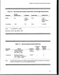 Methods
best, be accurate to within one-tenth of a degree Celsius. Temperature
probe systems are rarely linear over large temperature ranges and must be
checked against research-grade laboratory thermometers (APHA, 1989).
Salinity probe systems offer moderate accuracy but should be cross-checked
by discrete water samples analyzed by induction-type laboratory
salinometers (APHA, 1989). Two standard determinations should be made
before the start of each series of samples. In addition, one standard sample
should be analyzed to monitor instrument drift. It is recommended that
duplicate determinations be made for at least 10 percent of the samples
analyzed.
Many multiprobe in situ measurement systems incorporate depth
measurements by use of pressure transducers. The accuracy and precision
of such systems must be periodically checked. A pressure calibration can be
done in a laboratory pressure chamber. Daily calibration may be done in
calm waters of a known depth (e.g., inside a lagoon or a marina). Precision
is determined by multiple measurements at the same depth. Accuracy is
evaluated by comparison to measurements made with a heavily weighted line.
Instruments that measure turbidity require regular calibration. In situ
instruments are most accurately calibrated by the use of primary standards,
usually a carefully prepared suspension of Formalin or other approved
standard. Transmissometer-type instruments can be calibrated by
comparison to solutions of known total suspended solids. These solutions
should approximate the turbidity of the water that is to be sampled. For other
instruments, including those nephelometers or turbidity meters that measure
discrete samples, either on deck or in the laboratory, calibration using an
approved primary standard suspension is recommended (APHA, 1989).
Calibration in all cases should be conducted at the start of each series of
analyses and after each group of 10 successive samples. Duplicate
analyses should be conducted on at least 10 percent of the total number of
samples (U.S. EPA, 1987c).
Transmissometers can be calibrated in air and must be strictly cleaned.
A standard suspension of Formalin, prepared under closely defined
conditions, is used to calibrate the nephelometer (USEPA, 1983a, Method
180.1). The nephelometer should be calibrated at the start of each series of
analyses and after each group of 10 successive samples. Duplicate
analyses should be conducted on at least 10 percent of the total number of
samples (USEPA, 1987c).
Current meters should be calibrated before and after each major deployment
of instruments.
UNESCO (1988) presents details on the calibration of CTD instruments.
so
image:
Methods
best, be accurate to within one-tenth of a degree Celsius. Temperature
probe systems are rarely linear over large temperature ranges and must be
checked against research-grade laboratory thermometers (APHA, 1989).
Salinity probe systems offer moderate accuracy but should be cross-checked
by discrete water samples analyzed by induction-type laboratory
salinometers (APHA, 1989). Two standard determinations should be made
before the start of each series of samples. In addition, one standard sample
should be analyzed to monitor instrument drift. It is recommended that
duplicate determinations be made for at least 10 percent of the samples
analyzed.
Many multiprobe in situ measurement systems incorporate depth
measurements by use of pressure transducers. The accuracy and precision
of such systems must be periodically checked. A pressure calibration can be
done in a laboratory pressure chamber. Daily calibration may be done in
calm waters of a known depth (e.g., inside a lagoon or a marina). Precision
is determined by multiple measurements at the same depth. Accuracy is
evaluated by comparison to measurements made with a heavily weighted line.
Instruments that measure turbidity require regular calibration. In situ
instruments are most accurately calibrated by the use of primary standards,
usually a carefully prepared suspension of Formalin or other approved
standard. Transmissometer-type instruments can be calibrated by
comparison to solutions of known total suspended solids. These solutions
should approximate the turbidity of the water that is to be sampled. For other
instruments, including those nephelometers or turbidity meters that measure
discrete samples, either on deck or in the laboratory, calibration using an
approved primary standard suspension is recommended (APHA, 1989).
Calibration in all cases should be conducted at the start of each series of
analyses and after each group of 10 successive samples. Duplicate
analyses should be conducted on at least 10 percent of the total number of
samples (U.S. EPA, 1987c).
Transmissometers can be calibrated in air and must be strictly cleaned.
A standard suspension of Formalin, prepared under closely defined
conditions, is used to calibrate the nephelometer (USEPA, 1983a, Method
180.1). The nephelometer should be calibrated at the start of each series of
analyses and after each group of 10 successive samples. Duplicate
analyses should be conducted on at least 10 percent of the total number of
samples (USEPA, 1987c).
Current meters should be calibrated before and after each major deployment
of instruments.
UNESCO (1988) presents details on the calibration of CTD instruments.
so
image:
 Section 403 Procedural and Monitoring Guidance
• Fluorometer calibration performed prior to use with a series of prepared
concentrations, blanks, and spikes is recommended as a quality control
check (Wilson, 1986).
4.1.5 Statistical Design Considerations
Temporal Analyses
In general, one would expect to find temporal and spatial patterns in physical
characteristics. As a result, the primary purpose of measuring physical characteristics is
to describe what these patterns are (e.g., range, seasonal variations) and to determine
the primary physical mechanisms affecting the monitored area. As a result, statistical
comparisons between sampling locations and sampling periods are not common except
for turbidity. In this instance, the reader is referred to Section 4.2, Water Chemistry, for
analysis approaches that would be appropriate. All raw data should have error limits
associated with them to indicate the level of confidence in the data.
Tidal and seasonal variability in the distribution and magnitude of water column physical
characteristics is typically observed (Day et al., 1989). Time series analyses (e.g.,
temporal autocorrelation and spectral analyses) may be necessary to examine the
effects of the cyclical influences and/or filter out these cyclic forcing functions in order to
examine long-term temporal trends.
Graphical Representation
The physical characteristics data described in this section are typically summarized in
graphical form. The most common summary graphs include temperature-depth profiles,
salinity-depth profiles, and temperature-salinity plots. Physical oceanographers typically
analyze characteristic diagrams of water properties. The most common curve is a
temperature-salinity (T-S) plot.
Alternatively, horizontal sections (e.g., contour maps) of properties are useful for
displaying geographical distributions. Multiple physical characteristics may be displayed
by displacing one graph above the other. More details about analyzing characteristic
diagrams can be found in Pickard and Emery (1982).
Current data can be displayed in numerous fashions including stick plots, a time series
of rectangular components, and horizontal maps (Pickard and Emery, 1982). These
figures are typically plotted after periodic components have been removed through
spectral analysis, leaving only the residual nonperiodic components.
51
image:
Section 403 Procedural and Monitoring Guidance
• Fluorometer calibration performed prior to use with a series of prepared
concentrations, blanks, and spikes is recommended as a quality control
check (Wilson, 1986).
4.1.5 Statistical Design Considerations
Temporal Analyses
In general, one would expect to find temporal and spatial patterns in physical
characteristics. As a result, the primary purpose of measuring physical characteristics is
to describe what these patterns are (e.g., range, seasonal variations) and to determine
the primary physical mechanisms affecting the monitored area. As a result, statistical
comparisons between sampling locations and sampling periods are not common except
for turbidity. In this instance, the reader is referred to Section 4.2, Water Chemistry, for
analysis approaches that would be appropriate. All raw data should have error limits
associated with them to indicate the level of confidence in the data.
Tidal and seasonal variability in the distribution and magnitude of water column physical
characteristics is typically observed (Day et al., 1989). Time series analyses (e.g.,
temporal autocorrelation and spectral analyses) may be necessary to examine the
effects of the cyclical influences and/or filter out these cyclic forcing functions in order to
examine long-term temporal trends.
Graphical Representation
The physical characteristics data described in this section are typically summarized in
graphical form. The most common summary graphs include temperature-depth profiles,
salinity-depth profiles, and temperature-salinity plots. Physical oceanographers typically
analyze characteristic diagrams of water properties. The most common curve is a
temperature-salinity (T-S) plot.
Alternatively, horizontal sections (e.g., contour maps) of properties are useful for
displaying geographical distributions. Multiple physical characteristics may be displayed
by displacing one graph above the other. More details about analyzing characteristic
diagrams can be found in Pickard and Emery (1982).
Current data can be displayed in numerous fashions including stick plots, a time series
of rectangular components, and horizontal maps (Pickard and Emery, 1982). These
figures are typically plotted after periodic components have been removed through
spectral analysis, leaving only the residual nonperiodic components.
51
image:
 Methods
4.1.6
Use of Data
Data describing the physical parameters can be used to determine water column
stability, characterize oceanographic conditions in the discharge area, determine initial
dilution, assist in the prediction of plume behavior, identify the area impacted by the
discharge, and identify existing and potential problem areas for fish and sensitive life
stages of marine organisms (e.g., upwelling areas).
Salinity and temperature can be used, together with current speed and direction, to aid
in describing mass movement of diluted waste plumes to far-field sites where impacts
must be assessed (Wright, 1988). Furthermore, salinity, temperature, and currents are
used to assist in evaluating the results of benthic and other biological responses.
Current-speed data may be used to determine the distance from the outfall that the
sediment will travel before accumulating on the bottom.
Dye studies are particularly useful to evaluate the movement of the plume, the likelihood
that the plume will reach the shoreline or nearby biologically sensitive areas, the
potential for re-entrainment of previously discharged effluent, and the recirculation
potential under short-term influences for existing discharges, as well as the general
circulation patterns in the vicinity of discharge sites (USEPA, 1982a).
Physical characteristics data are used to calibrate and validate hydrodynamic and
dispersion plume models (Davis, 1988; Leighton et al., 1988; USEPA, 1982a). For
relocated or proposed discharges, numerical circulation and transport models are the
most useful methods for assessing the effects of ambient currents and stratification on
dispersion and transport of the waste field and for estimating the potential for
recirculation of previously discharged effluent. Statistical analysis can be performed to
forecast plume direction under varying physical conditions.
Turbidity data can be used to estimate the reduction in light transmittance. Reduction of
the depth to which sunlight penetrates, due to an increase in turbidity, will cause a
decrease in the compensation depth of phytoplankton, resulting in reduced biological
growth (Thomann and Mueller, 1987).
4.1.7 Summary and Recommendations
Rationale
Most chemical and biological processes in the marine environment are
affected, either directly or indirectly, by the physical characteristics of the
marine environment.
52
image:
Methods
4.1.6
Use of Data
Data describing the physical parameters can be used to determine water column
stability, characterize oceanographic conditions in the discharge area, determine initial
dilution, assist in the prediction of plume behavior, identify the area impacted by the
discharge, and identify existing and potential problem areas for fish and sensitive life
stages of marine organisms (e.g., upwelling areas).
Salinity and temperature can be used, together with current speed and direction, to aid
in describing mass movement of diluted waste plumes to far-field sites where impacts
must be assessed (Wright, 1988). Furthermore, salinity, temperature, and currents are
used to assist in evaluating the results of benthic and other biological responses.
Current-speed data may be used to determine the distance from the outfall that the
sediment will travel before accumulating on the bottom.
Dye studies are particularly useful to evaluate the movement of the plume, the likelihood
that the plume will reach the shoreline or nearby biologically sensitive areas, the
potential for re-entrainment of previously discharged effluent, and the recirculation
potential under short-term influences for existing discharges, as well as the general
circulation patterns in the vicinity of discharge sites (USEPA, 1982a).
Physical characteristics data are used to calibrate and validate hydrodynamic and
dispersion plume models (Davis, 1988; Leighton et al., 1988; USEPA, 1982a). For
relocated or proposed discharges, numerical circulation and transport models are the
most useful methods for assessing the effects of ambient currents and stratification on
dispersion and transport of the waste field and for estimating the potential for
recirculation of previously discharged effluent. Statistical analysis can be performed to
forecast plume direction under varying physical conditions.
Turbidity data can be used to estimate the reduction in light transmittance. Reduction of
the depth to which sunlight penetrates, due to an increase in turbidity, will cause a
decrease in the compensation depth of phytoplankton, resulting in reduced biological
growth (Thomann and Mueller, 1987).
4.1.7 Summary and Recommendations
Rationale
Most chemical and biological processes in the marine environment are
affected, either directly or indirectly, by the physical characteristics of the
marine environment.
52
image:
 Section 403 Procedural and Monitoring Guidance
• Physical data can be used to determine plume and sediment movement
(hydrodynamics and fate and transport modeling) and to provide ancillary
information to interpret other water chemistry variables.
• National temperature criteria to ensure protection of the characteristic
indigenous marine community have been established in the "Gold Book" for
temperature (USEPA, 1986d).
Monitoring Design Considerations
• In general, data on temperature, salinity, density, turbidity, and depth (depth
of sample and depth to bottom) should be collected at every station location.
Sufficient data should be collected in the vertical profile for temperature and
salinity. Common practice is to collect one data point per meter of depth.
• The number and location of current measurements should be based on the
complexity of the circulation patterns and the effluent characteristics.
Stations should be located in the vicinity of the zone of initial dilution (ZID)
boundary, at control sites, and in impacted areas.
• If a mathematical model will be used to assess the effects of ambient physical
characteristics and the fate and transport of the discharged effluent, the
monitoring program should be designed to provide the model with the
required forcing boundary data.
• Data should be collected at a frequency sufficient to characterize seasonal
patterns and critical periods (e.g., time of seasonal maximum and minimum
stratification, low net circulation, time and duration of coastal upwelling, and
exceptional biological activity).
• Estimates of the error should be made with each variable.
Analytical Methods Considerations
• Temperature measurements may be made with:
- Mercury-filled or dial-type centigrade thermometer
- Thermistor
- Reverse thermometer
- Bathythermograph
- CTD instrumentation
• Salinity measurements are preferably made with:
- Conductivity cells (CTD instruments)
53
image:
Section 403 Procedural and Monitoring Guidance
• Physical data can be used to determine plume and sediment movement
(hydrodynamics and fate and transport modeling) and to provide ancillary
information to interpret other water chemistry variables.
• National temperature criteria to ensure protection of the characteristic
indigenous marine community have been established in the "Gold Book" for
temperature (USEPA, 1986d).
Monitoring Design Considerations
• In general, data on temperature, salinity, density, turbidity, and depth (depth
of sample and depth to bottom) should be collected at every station location.
Sufficient data should be collected in the vertical profile for temperature and
salinity. Common practice is to collect one data point per meter of depth.
• The number and location of current measurements should be based on the
complexity of the circulation patterns and the effluent characteristics.
Stations should be located in the vicinity of the zone of initial dilution (ZID)
boundary, at control sites, and in impacted areas.
• If a mathematical model will be used to assess the effects of ambient physical
characteristics and the fate and transport of the discharged effluent, the
monitoring program should be designed to provide the model with the
required forcing boundary data.
• Data should be collected at a frequency sufficient to characterize seasonal
patterns and critical periods (e.g., time of seasonal maximum and minimum
stratification, low net circulation, time and duration of coastal upwelling, and
exceptional biological activity).
• Estimates of the error should be made with each variable.
Analytical Methods Considerations
• Temperature measurements may be made with:
- Mercury-filled or dial-type centigrade thermometer
- Thermistor
- Reverse thermometer
- Bathythermograph
- CTD instrumentation
• Salinity measurements are preferably made with:
- Conductivity cells (CTD instruments)
53
image:
 Methods
• Density measurements are preferably made with:
- Indirect methods (function of salinity, temperature, and pressure)
• Depth measurements are preferably made with:
- Hydrostatic pressure techniques
• Turbidity measurements may be made with:
- Light transmissometer
- Secchi disc
• Current measurements may be made with:
- Eulerian methods - propeller-type meters, electromagnetic meters,
acoustic-doppler meters, etc.
- Lagrangian methods - drogues, surface drifters, etc.
• Plume studies may be performed with:
- Fluorescent dyes injected into the waste stream
- Emerging acoustic technologies
QA/QC Considerations
• A multistep QA/QC program must be implemented to verify that all
calibrations were conducted and properly applied to data and, where
possible, to ensure historical verification.
• All equipment must be calibrated regularly.
• Blank, spike recovery, and replicate analyses are recommended quality
control checks for those parameters to which they can be applied.
• For replicates, a minimum of three repetitions is required for statistical
significance.
Statistical Design Considerations
• The primary purpose is to describe the patterns of physical characteristics
(e.g., range, seasonal variations) and to determine the primary physical
mechanisms affecting the monitored area. As a result, statistical
comparisons between sampling locations and sampling periods are not
common except for turbidity.
• Common graphical summaries include:
54
image:
Methods
• Density measurements are preferably made with:
- Indirect methods (function of salinity, temperature, and pressure)
• Depth measurements are preferably made with:
- Hydrostatic pressure techniques
• Turbidity measurements may be made with:
- Light transmissometer
- Secchi disc
• Current measurements may be made with:
- Eulerian methods - propeller-type meters, electromagnetic meters,
acoustic-doppler meters, etc.
- Lagrangian methods - drogues, surface drifters, etc.
• Plume studies may be performed with:
- Fluorescent dyes injected into the waste stream
- Emerging acoustic technologies
QA/QC Considerations
• A multistep QA/QC program must be implemented to verify that all
calibrations were conducted and properly applied to data and, where
possible, to ensure historical verification.
• All equipment must be calibrated regularly.
• Blank, spike recovery, and replicate analyses are recommended quality
control checks for those parameters to which they can be applied.
• For replicates, a minimum of three repetitions is required for statistical
significance.
Statistical Design Considerations
• The primary purpose is to describe the patterns of physical characteristics
(e.g., range, seasonal variations) and to determine the primary physical
mechanisms affecting the monitored area. As a result, statistical
comparisons between sampling locations and sampling periods are not
common except for turbidity.
• Common graphical summaries include:
54
image:
 Section 403 Procedural and Monitoring Guidance
Temperature-depth profiles, salinity-depth profiles, and
temperature-salinity plots.
Horizontal sections (i.e., contour maps) of properties.
Time series data, which are often displayed as a function of time with
multiple physical characteristics displayed by placing one graph above the
other.
Current data, which can be displayed with stick plots, a time series of
rectangular components, and horizontal maps.
Use of Data
Physical characteristics are used to determine water column stability, to
characterize oceanographic conditions in the discharge area, to determine
initial dilution, to assist in the prediction of plume behavior, to identify the area
impacted by the discharge, and to identify existing and potential problem
areas for fish and sensitive life stages of marine organisms (e.g., upwelling
areas).
Statistical studies can be performed to forecast plume direction under varying
physical conditions.
Dye studies are particularly useful to evaluate the movement of the plume,
the likelihood that the plume will reach the shoreline or nearby biologically
sensitive areas, the potential for re-entrainment of previously discharged
effluent, and the recirculation potential under short-term influences for
existing discharges, as well as the general circulation patterns in the vicinity
of discharge sites.
Physical characteristics data are used to calibrate and validate hydrodynamic
and dispersion plume models.
Turbidity can be used to estimate the reduction of light transmittance.
Reduction of the depth to which sunlight penetrates, due to an increase in
turbidity, can reduce biological community growth.
55
image:
Section 403 Procedural and Monitoring Guidance
Temperature-depth profiles, salinity-depth profiles, and
temperature-salinity plots.
Horizontal sections (i.e., contour maps) of properties.
Time series data, which are often displayed as a function of time with
multiple physical characteristics displayed by placing one graph above the
other.
Current data, which can be displayed with stick plots, a time series of
rectangular components, and horizontal maps.
Use of Data
Physical characteristics are used to determine water column stability, to
characterize oceanographic conditions in the discharge area, to determine
initial dilution, to assist in the prediction of plume behavior, to identify the area
impacted by the discharge, and to identify existing and potential problem
areas for fish and sensitive life stages of marine organisms (e.g., upwelling
areas).
Statistical studies can be performed to forecast plume direction under varying
physical conditions.
Dye studies are particularly useful to evaluate the movement of the plume,
the likelihood that the plume will reach the shoreline or nearby biologically
sensitive areas, the potential for re-entrainment of previously discharged
effluent, and the recirculation potential under short-term influences for
existing discharges, as well as the general circulation patterns in the vicinity
of discharge sites.
Physical characteristics data are used to calibrate and validate hydrodynamic
and dispersion plume models.
Turbidity can be used to estimate the reduction of light transmittance.
Reduction of the depth to which sunlight penetrates, due to an increase in
turbidity, can reduce biological community growth.
55
image:
 Methods
4.2
WATER CHEMISTRY
Monitoring of water chemistry parameters is conducted to evaluate the quality of
receiving waters. Commonly employed EPA methods were intended for use in the
detection of pollutants at high concentrations relative to those usually found in natural
waters. Much attention has been devoted recently to the need for the development of
more appropriate methods, but evaluation and validation of these methods have not
been conducted on a wide scale. Until these and other QA measures are developed,
the traditional EPA methods are generally the methods of choice for the analysis of
water quality. Recommended Protocols for Measuring Selected Environmental
Variables in Puget Sound (USEPA, 1986-1991) contains discussions of QA/QC
concerns, sampling considerations, and recommended instrumental methods. The
Compendium of Methods for Marine and Estuarine Environmental Studies (USEPA,
1990b) includes a number of method variations for nitrogen species, phosphorus, and
chlorophyll.
4.2.1
Rationale
Of the 10 guidelines used to determine unreasonable degradation or irreparable harm,
the following can be assessed by evaluating the water chemistry:
• Potential transport of the pollutants by biological, physical, or chemical
processes;
• Potential direct or indirect impacts on human health; and
• Marine water quality criteria.
The presence of toxic material in marine waters due to point source discharges can
have adverse ecological and human health effects. Near-field monitoring of chemical
concentrations can provide a spatial and temporal record of contamination in the water
column. Water quality chemistry measurements should be made as part of a monitoring
program to assess the effectiveness of the permit guidelines in preventing unreasonable
degradation of or irreparable harm to the marine environment.
4.2.2 Monitoring Design Considerations
SelectiorLof Analytes
The chemicals that should be included in the monitoring program are those chemicals
known or suspected to be in the discharge, as well as possible by-products. Even
though potentially toxic compounds in the discharge may not be fully known, the
objectives of the program must be clearly defined. It may be necessary at the beginning
of the program to conduct an analysis for all chemicals on the EPA-defined Priority
Pollutant, Hazardous Substance, or Target Compound/Analyte Lists to determine which
are present; however, detection in the environment does not always correlate with
image:
Methods
4.2
WATER CHEMISTRY
Monitoring of water chemistry parameters is conducted to evaluate the quality of
receiving waters. Commonly employed EPA methods were intended for use in the
detection of pollutants at high concentrations relative to those usually found in natural
waters. Much attention has been devoted recently to the need for the development of
more appropriate methods, but evaluation and validation of these methods have not
been conducted on a wide scale. Until these and other QA measures are developed,
the traditional EPA methods are generally the methods of choice for the analysis of
water quality. Recommended Protocols for Measuring Selected Environmental
Variables in Puget Sound (USEPA, 1986-1991) contains discussions of QA/QC
concerns, sampling considerations, and recommended instrumental methods. The
Compendium of Methods for Marine and Estuarine Environmental Studies (USEPA,
1990b) includes a number of method variations for nitrogen species, phosphorus, and
chlorophyll.
4.2.1
Rationale
Of the 10 guidelines used to determine unreasonable degradation or irreparable harm,
the following can be assessed by evaluating the water chemistry:
• Potential transport of the pollutants by biological, physical, or chemical
processes;
• Potential direct or indirect impacts on human health; and
• Marine water quality criteria.
The presence of toxic material in marine waters due to point source discharges can
have adverse ecological and human health effects. Near-field monitoring of chemical
concentrations can provide a spatial and temporal record of contamination in the water
column. Water quality chemistry measurements should be made as part of a monitoring
program to assess the effectiveness of the permit guidelines in preventing unreasonable
degradation of or irreparable harm to the marine environment.
4.2.2 Monitoring Design Considerations
SelectiorLof Analytes
The chemicals that should be included in the monitoring program are those chemicals
known or suspected to be in the discharge, as well as possible by-products. Even
though potentially toxic compounds in the discharge may not be fully known, the
objectives of the program must be clearly defined. It may be necessary at the beginning
of the program to conduct an analysis for all chemicals on the EPA-defined Priority
Pollutant, Hazardous Substance, or Target Compound/Analyte Lists to determine which
are present; however, detection in the environment does not always correlate with
image:
 Section 403 Procedural and Monitoring Guidance
biological risks and effects. Furthermore, many of the chemicals that pose risks to
marine systems are hydrophobia Water column monitoring for hydrophobic chemicals
may indicate concentrations that are several orders of magnitude below concentrations
in sediments and biota. Unless compelling site-specific conditions warrant otherwise,
water column monitoring for hydrophobic chemicals is not recommended. Limitations in
analytical methodology, modeling techniques, and toxicological data restrict the
usefulness of the resulting data. In some cases, levels of contaminants that are of
concern to the health of organisms are below the lowest limit of detection of the best
available analytical methodology.
Sampling Considerations
Selection of sampling locations and choice of sampling techniques are crucial decisions
to be made before the sampling effort is initiated. Recommended Protocols for
Measuring Selected Environmental Variables in Puget Sound (USEPA, 1986-1991)
contains discussions of quality assurance requirements and sampling considerations
that are applicable to water quality monitoring. Sampling must incorporate sites within
the zone of initial dilution, extending out to areas of low contaminant concentration and
farther to unaffected areas to address the complete spatial variability.
Water column sampling design must consider not only the horizontal location of the
sampling stations, but also the vertical location within the water column and the time of
sample collection. Because the majority of chemical analyses are performed, by
necessity, on discrete samples, consideration should be given to the number of depths
at which samples are collected. Obviously, such decisions will be based on site-specific
characteristics, such as water depth, contaminants of concern, suspected sources, and
the sensitivity or importance of local biota. Costs related to the laboratory analyses
should also be weighed against the number of samples desired.
Water Column Sampling Equipment
Water column samples are frequently collected using bottle samplers. These are simple
devices, usually consisting of cylindrical tubes with stoppers at each end and a closing
device that is activated by an electrical signal. Each bottle samples a discrete parcel of
water at a designated depth. Multiple samplers are fixed on a rosette frame in order that
several depths may be sampled during one cast and/or that replicate samples may be
collected at a particular depth. The most commonly used bottle samplers include the
Kemmerer, Van Dorn, Niskin, and Nansen samplers (USEPA, 1987c). Alternatively, a
pump may be used to sample the water column (USEPA, 1987c).
Depending on the depth of the water at the sampling site, samples should be taken at a
minimum of four depths in the vertical profile: (1) 1 meter below the surface, (2) 1 meter
above the bottom, (3) 1 meter above the pycnocline, and (4) 1 meter below the
57
image:
Section 403 Procedural and Monitoring Guidance
biological risks and effects. Furthermore, many of the chemicals that pose risks to
marine systems are hydrophobia Water column monitoring for hydrophobic chemicals
may indicate concentrations that are several orders of magnitude below concentrations
in sediments and biota. Unless compelling site-specific conditions warrant otherwise,
water column monitoring for hydrophobic chemicals is not recommended. Limitations in
analytical methodology, modeling techniques, and toxicological data restrict the
usefulness of the resulting data. In some cases, levels of contaminants that are of
concern to the health of organisms are below the lowest limit of detection of the best
available analytical methodology.
Sampling Considerations
Selection of sampling locations and choice of sampling techniques are crucial decisions
to be made before the sampling effort is initiated. Recommended Protocols for
Measuring Selected Environmental Variables in Puget Sound (USEPA, 1986-1991)
contains discussions of quality assurance requirements and sampling considerations
that are applicable to water quality monitoring. Sampling must incorporate sites within
the zone of initial dilution, extending out to areas of low contaminant concentration and
farther to unaffected areas to address the complete spatial variability.
Water column sampling design must consider not only the horizontal location of the
sampling stations, but also the vertical location within the water column and the time of
sample collection. Because the majority of chemical analyses are performed, by
necessity, on discrete samples, consideration should be given to the number of depths
at which samples are collected. Obviously, such decisions will be based on site-specific
characteristics, such as water depth, contaminants of concern, suspected sources, and
the sensitivity or importance of local biota. Costs related to the laboratory analyses
should also be weighed against the number of samples desired.
Water Column Sampling Equipment
Water column samples are frequently collected using bottle samplers. These are simple
devices, usually consisting of cylindrical tubes with stoppers at each end and a closing
device that is activated by an electrical signal. Each bottle samples a discrete parcel of
water at a designated depth. Multiple samplers are fixed on a rosette frame in order that
several depths may be sampled during one cast and/or that replicate samples may be
collected at a particular depth. The most commonly used bottle samplers include the
Kemmerer, Van Dorn, Niskin, and Nansen samplers (USEPA, 1987c). Alternatively, a
pump may be used to sample the water column (USEPA, 1987c).
Depending on the depth of the water at the sampling site, samples should be taken at a
minimum of four depths in the vertical profile: (1) 1 meter below the surface, (2) 1 meter
above the bottom, (3) 1 meter above the pycnocline, and (4) 1 meter below the
57
image:
 Methods
pycnocline. If the waters are too shallow or no stratification occurs, it would be
appropriate to take the latter two samples at evenly spaced distances between the top
and bottom samples.
Caged Organisms
The California Mussel Watch Program and the National Oceanic and Atmospheric
Administration (NOAA) Status and Trends Program have employed the use of caged
transplanted mussels to monitor bioaccumulation of toxic chemicals over space and time
(Ladd et al., 1984; Goldberg et al., 1978). Caged sentinel species offer several
advantages:
• They concentrate contaminants (up to 102-105 fold vs. ambient waters),
facilitating laboratory analyses of contaminant concentrations.
• They provide a means of temporally integrating water quality conditions.
• They provide an assessment of biological availability of water column
contaminants.
• They may be deployed and maintained in a number of diverse locales.
However, the disadvantages of caged organisms include the cost of transplanting
organisms, the possibility of loss of the cage/buoy system, and the possibility of
introducing a "nuisance" species. Species have different bioaccumulation potentials for
various contaminants. It is recommended that multiple sentinel species be deployed to
ensure that a number of contaminants are sufficiently evaluated and a comprehensive
characterization of water contaminants is conducted. Unfortunately, formulations that
would allow comparisons of bioaccumulation data between different species and/or
different tissues types have not yet been developed and comparison of tissue burdens
among the species is not acceptable. Thus, it is essential that monitoring design
elements be standardized to allow for comparisons among studies.
4.2.3 Analytical Methods Considerations
Questions to be considered during the choice of an appropriate analytical method
include the parameters of interest, desired detection limits, sample size requirements or
restrictions, methods of preservation, technical and practical holding times, and matrix
interferences (especially from saline water). D'Elia et al. (1989) discuss the common
analytical problems encountered during monitoring analyses of water samples.
Selection of appropriate methods should be based on a compromise between full-scan
analyses, which are economical but cannot provide optimal sensitivity for all
compounds, and alternative methods that are more sensitive for specific compounds but
58
image:
Methods
pycnocline. If the waters are too shallow or no stratification occurs, it would be
appropriate to take the latter two samples at evenly spaced distances between the top
and bottom samples.
Caged Organisms
The California Mussel Watch Program and the National Oceanic and Atmospheric
Administration (NOAA) Status and Trends Program have employed the use of caged
transplanted mussels to monitor bioaccumulation of toxic chemicals over space and time
(Ladd et al., 1984; Goldberg et al., 1978). Caged sentinel species offer several
advantages:
• They concentrate contaminants (up to 102-105 fold vs. ambient waters),
facilitating laboratory analyses of contaminant concentrations.
• They provide a means of temporally integrating water quality conditions.
• They provide an assessment of biological availability of water column
contaminants.
• They may be deployed and maintained in a number of diverse locales.
However, the disadvantages of caged organisms include the cost of transplanting
organisms, the possibility of loss of the cage/buoy system, and the possibility of
introducing a "nuisance" species. Species have different bioaccumulation potentials for
various contaminants. It is recommended that multiple sentinel species be deployed to
ensure that a number of contaminants are sufficiently evaluated and a comprehensive
characterization of water contaminants is conducted. Unfortunately, formulations that
would allow comparisons of bioaccumulation data between different species and/or
different tissues types have not yet been developed and comparison of tissue burdens
among the species is not acceptable. Thus, it is essential that monitoring design
elements be standardized to allow for comparisons among studies.
4.2.3 Analytical Methods Considerations
Questions to be considered during the choice of an appropriate analytical method
include the parameters of interest, desired detection limits, sample size requirements or
restrictions, methods of preservation, technical and practical holding times, and matrix
interferences (especially from saline water). D'Elia et al. (1989) discuss the common
analytical problems encountered during monitoring analyses of water samples.
Selection of appropriate methods should be based on a compromise between full-scan
analyses, which are economical but cannot provide optimal sensitivity for all
compounds, and alternative methods that are more sensitive for specific compounds but
58
image:
 Section 403 Procedural and Monitoring Guidance
can result in higher analytical costs. A list of analytical techniques is presented in Table
4-8. Table 4-9 shows which technique is appropriate for detecting a specific organic
contaminant.
Dissolved Oxygen
The titrimetric, or Winkler, method is the first method of choice for the measurement of
dissolved oxygen (USEPA, 1983a). The membrane electrode method (360.1) is
recommended for samples containing interferents such as sulfur compounds, chlorine,
free iodine, color, turbidity, or biological floes, and also when continuous monitoring is
planned (USEPA, 1983a).
Nutrients
Nutrients such as ammonia nitrogen, total Kjeldahl nitrogen, nitrate-nitrite nitrogen, and
phosphorus are determined by spectrophotometric measurements using a segmented
continuous flow analyzer, where samples and reagents are continuously added in
sequence separated by air bubbles and pumped through glass tubing (USEPA, 1983a).
Successive analyses can be accomplished in less time than would be required by
manual methods because each analysis is not carried to completion, but is brought to
the same stage of development and exposure by the timing of the stream flow through
the system. Possible interferences include suspended solids, metal ions, and residual
chlorine.
Ammonia nitrogen is determined by treating the samples with alkaline phenol and
hypochlorite to produce indophenol blue, which is intensified with sodium nitroprusside.
Standard solutions should be made up using substitute sea water to approximate the
matrix of the samples (USEPA, 1983a). Total Kjeldahl nitrogen is defined as the sum of
free ammonia and organic nitrogen compounds, which are converted to ammonium
sulfate under the conditions of digestion (USEPA, 1983a). Sulfates react with nitrogen
compounds of biological origin, but may not convert nitrogenous compounds of some
industrial wastes. For the determination of nitrate-nitrite nitrogen, a filtered sample is
passed through a granulated copper-cadmium column to reduce any nitrate to nitrite
(USEPA, 1983a). The nitrite is then transformed to a highly colored azo dye, which is
measured spectrophotometrically.
Total phosphorus is determined by heating the samples in the presence of sulfates, then
cooling and measuring spectrophotometrically (USEPA, 1983a).
The fluorometric method for chlorophyll a is more sensitive than the spectrophotometric
method. The sample is subjected to an excitation wavelength, and the fluorescence is
measured at a second emission wavelength (APHA, 1989). The greatest uncertainty in
the method is the choice of reference standard. High performance liquid
59
image:
Section 403 Procedural and Monitoring Guidance
can result in higher analytical costs. A list of analytical techniques is presented in Table
4-8. Table 4-9 shows which technique is appropriate for detecting a specific organic
contaminant.
Dissolved Oxygen
The titrimetric, or Winkler, method is the first method of choice for the measurement of
dissolved oxygen (USEPA, 1983a). The membrane electrode method (360.1) is
recommended for samples containing interferents such as sulfur compounds, chlorine,
free iodine, color, turbidity, or biological floes, and also when continuous monitoring is
planned (USEPA, 1983a).
Nutrients
Nutrients such as ammonia nitrogen, total Kjeldahl nitrogen, nitrate-nitrite nitrogen, and
phosphorus are determined by spectrophotometric measurements using a segmented
continuous flow analyzer, where samples and reagents are continuously added in
sequence separated by air bubbles and pumped through glass tubing (USEPA, 1983a).
Successive analyses can be accomplished in less time than would be required by
manual methods because each analysis is not carried to completion, but is brought to
the same stage of development and exposure by the timing of the stream flow through
the system. Possible interferences include suspended solids, metal ions, and residual
chlorine.
Ammonia nitrogen is determined by treating the samples with alkaline phenol and
hypochlorite to produce indophenol blue, which is intensified with sodium nitroprusside.
Standard solutions should be made up using substitute sea water to approximate the
matrix of the samples (USEPA, 1983a). Total Kjeldahl nitrogen is defined as the sum of
free ammonia and organic nitrogen compounds, which are converted to ammonium
sulfate under the conditions of digestion (USEPA, 1983a). Sulfates react with nitrogen
compounds of biological origin, but may not convert nitrogenous compounds of some
industrial wastes. For the determination of nitrate-nitrite nitrogen, a filtered sample is
passed through a granulated copper-cadmium column to reduce any nitrate to nitrite
(USEPA, 1983a). The nitrite is then transformed to a highly colored azo dye, which is
measured spectrophotometrically.
Total phosphorus is determined by heating the samples in the presence of sulfates, then
cooling and measuring spectrophotometrically (USEPA, 1983a).
The fluorometric method for chlorophyll a is more sensitive than the spectrophotometric
method. The sample is subjected to an excitation wavelength, and the fluorescence is
measured at a second emission wavelength (APHA, 1989). The greatest uncertainty in
the method is the choice of reference standard. High performance liquid
59
image:
 Methods
jUjtiJilL..* *~t t v
Table 4-8. List of Analytical Techniques
DISSOLVED OXYGEN
• Winkler Titration
• Membrane Electrode
NUTRIENTS
• Continuous Flow Spectrophotometry
- Ammonia Nitrogen
- Total Kjeldahl Nitrogen
- Nitrate-Nitrite Nitrogen
- Total Phosphorus
• Fluorescence Spectrometry
- Chlorophyll a
• High Performance Liquid Chromatography (HPLC)
TRACE METALS
• Atomic Absorption Spectrophotometry (AAS)
- flame
- graphite furnace (GFAAS)
- cold vapor
- gaseous hydride (HYDAAS)
• Inductively Coupled Plasma Emission
Spectrometry (ICP)
ORGANICS
• Gas Chromatography
- with electron capture detection (GC/ECD)
- with mass Spectrometry (GC/MS)
• Liquid Chromatography
- with mass Spectrometry (LC/MS)
USEPA method 360.2
USEPA method 360.1
USEPA method 350.1
USEPA method 351.2
USEPA method 353.2
USEPA method 365.4
Standard Method 10200
USEPA 200 series methods
USEPA method 200.7
USEPA 500/600 series methods
Chromatography (HPLC) is the most accurate of the methods used for the analysis of
chlorophyll (since all forms can be separately quantitated); however, it is also the most
expensive.
60
image:
Methods
jUjtiJilL..* *~t t v
Table 4-8. List of Analytical Techniques
DISSOLVED OXYGEN
• Winkler Titration
• Membrane Electrode
NUTRIENTS
• Continuous Flow Spectrophotometry
- Ammonia Nitrogen
- Total Kjeldahl Nitrogen
- Nitrate-Nitrite Nitrogen
- Total Phosphorus
• Fluorescence Spectrometry
- Chlorophyll a
• High Performance Liquid Chromatography (HPLC)
TRACE METALS
• Atomic Absorption Spectrophotometry (AAS)
- flame
- graphite furnace (GFAAS)
- cold vapor
- gaseous hydride (HYDAAS)
• Inductively Coupled Plasma Emission
Spectrometry (ICP)
ORGANICS
• Gas Chromatography
- with electron capture detection (GC/ECD)
- with mass Spectrometry (GC/MS)
• Liquid Chromatography
- with mass Spectrometry (LC/MS)
USEPA method 360.2
USEPA method 360.1
USEPA method 350.1
USEPA method 351.2
USEPA method 353.2
USEPA method 365.4
Standard Method 10200
USEPA 200 series methods
USEPA method 200.7
USEPA 500/600 series methods
Chromatography (HPLC) is the most accurate of the methods used for the analysis of
chlorophyll (since all forms can be separately quantitated); however, it is also the most
expensive.
60
image:
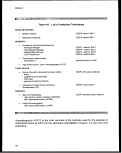 Section 403 Procedural and Monitoring Guidance
Table 4-9. USEPA Organic Contamination Detection Techniques
USEPA Method3
Contaminant Type
Method
601
602
603
604
606
608
609
610
611
614
624
625
F'urgeable Halocarbons
F'urgeable Aromatics
Acrolein/Acrylonitrile
F'henols
F'hthalate Esters
F'CBs and Organochlorine Pesticides
Nitroaromatics and Cyclic Ketones
Polycyclic Aromatic Hydrocarbons
Haloethers
Organophosphorous Pesticides
Volatile Organics
Semivolatile Organics
GC-ELCD
GC-PID
GC-FIDandPID
GC-FID
GC-ECD
GC-ECD
GC-FID-ECD
HPLC-UV-FL or GC-FID
GC-ECD
GC-FPD or NPD
GC-MS
GC-MS
1 USEPA, 1983a.
Trace Metals
The choice of analytical method for trace metal analysis is determined by the required
detection limit. Inductively coupled plasma emission spectrometry (ICP) allows the
simultaneous measurement of several elements; however, the achievable detection
limits are usually not as low as those obtained by graphite furnace or hydride atomic
absorption spectrophometry (AA). The combination of AA and ICP is the recommended
analytical method for detection of metals since no technique is best for all elements.
Cold vapor AA is the recommended technique for the analysis of mercury.
Graphite furnace AA is more sensitive than flame AA or ICP but is more subject to
matrix and spectral interferences. Such interferences result in potential quality control
problems during the analyses and uncertainties in the resulting data. Because of the
lower concentrations that can be seen by graphite furnace AA, particular caution must
be taken with regard to laboratory contamination. The concentration of each element is
determined by a separate analysis, making the analysis of a large number of
contaminant metals both labor-intensive and relatively expensive compared to ICP. AA
61
image:
Section 403 Procedural and Monitoring Guidance
Table 4-9. USEPA Organic Contamination Detection Techniques
USEPA Method3
Contaminant Type
Method
601
602
603
604
606
608
609
610
611
614
624
625
F'urgeable Halocarbons
F'urgeable Aromatics
Acrolein/Acrylonitrile
F'henols
F'hthalate Esters
F'CBs and Organochlorine Pesticides
Nitroaromatics and Cyclic Ketones
Polycyclic Aromatic Hydrocarbons
Haloethers
Organophosphorous Pesticides
Volatile Organics
Semivolatile Organics
GC-ELCD
GC-PID
GC-FIDandPID
GC-FID
GC-ECD
GC-ECD
GC-FID-ECD
HPLC-UV-FL or GC-FID
GC-ECD
GC-FPD or NPD
GC-MS
GC-MS
1 USEPA, 1983a.
Trace Metals
The choice of analytical method for trace metal analysis is determined by the required
detection limit. Inductively coupled plasma emission spectrometry (ICP) allows the
simultaneous measurement of several elements; however, the achievable detection
limits are usually not as low as those obtained by graphite furnace or hydride atomic
absorption spectrophometry (AA). The combination of AA and ICP is the recommended
analytical method for detection of metals since no technique is best for all elements.
Cold vapor AA is the recommended technique for the analysis of mercury.
Graphite furnace AA is more sensitive than flame AA or ICP but is more subject to
matrix and spectral interferences. Such interferences result in potential quality control
problems during the analyses and uncertainties in the resulting data. Because of the
lower concentrations that can be seen by graphite furnace AA, particular caution must
be taken with regard to laboratory contamination. The concentration of each element is
determined by a separate analysis, making the analysis of a large number of
contaminant metals both labor-intensive and relatively expensive compared to ICP. AA
61
image:
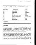 Methods
methods may, however, be cost-effective for the analysis of a few metals over a large
number of samples. It should be noted that "ultraclean" sampling and analytical
techniques should be used for trace metal samples in open ocean waters.
Semivolatile Organic Compounds
Analysis of semivolatile organic compounds involves a solvent extraction of the sample,
cleanup of the extract, gas chromatographic (GC) separation, and quantitation. There
are two gas chromatography/mass spectrometry (GC/MS) options for detecting
extractable organic compounds: internal standard and isotope dilution. The isotope
dilution technique, which requires spiking the sample with a mixture of stable
isotope-labeled analogs of the analytes, is recommended because reliable recovery
corrections can be made for each analyte with a labeled analog or a chemically similar
analog. This method is more expensive and less widely employed than the internal
standard method, which is the current method of choice in EPA's Contract Laboratory
Program. Mass spectrometry provides positive compound identification by comparison
of both retention time and spectral patterns with standard compounds.
Many organic compounds can be identified by gas chromatography/electron capture
detection (GC/ECD) analysis. GC/ECD provides greater sensitivity (lower detection
limits) relative to GC/MS; however, GC/ECD does not provide positive compound
identification. Since the identity of a compound is determined solely by matching
retention time with that of a standard, confirmation of the initial identity of the compound
on a second GC column is required for confidence in the reliability of the qualitative
identification of the compound. When a compound is present at a high enough
concentration, its identity should be confirmed by the use of GC/MS. GD/ECD is the
method of choice for pesticides and PCBs. Glass capillary GC achieves a much higher
degree of resolution in the analysis of the PCB congeners than the standard packed
column methods; however, few labs regularly employ this specialized technique. The
liquid chromatography/mass spectrometry (LC/MS) method is being developed for the
detection and quantitation of nonvolatile organic compounds.
Volatile Organic Compounds
The purge-and-trap GC/MS technique is commonly employed for detecting volatile
organic compounds in water. As in the case of semivolatiles, GC/ECD may be used to
achieve lower detection limits, although this introduces a level of uncertainty to the
qualitative identification of compounds. The isotope dilution technique is recommended
if the Data Quality Objectives (DQOs) of the monitoring program require accurate
quantitation of each compound. This technique, however, carries additional analytical
time and expense.
62
image:
Methods
methods may, however, be cost-effective for the analysis of a few metals over a large
number of samples. It should be noted that "ultraclean" sampling and analytical
techniques should be used for trace metal samples in open ocean waters.
Semivolatile Organic Compounds
Analysis of semivolatile organic compounds involves a solvent extraction of the sample,
cleanup of the extract, gas chromatographic (GC) separation, and quantitation. There
are two gas chromatography/mass spectrometry (GC/MS) options for detecting
extractable organic compounds: internal standard and isotope dilution. The isotope
dilution technique, which requires spiking the sample with a mixture of stable
isotope-labeled analogs of the analytes, is recommended because reliable recovery
corrections can be made for each analyte with a labeled analog or a chemically similar
analog. This method is more expensive and less widely employed than the internal
standard method, which is the current method of choice in EPA's Contract Laboratory
Program. Mass spectrometry provides positive compound identification by comparison
of both retention time and spectral patterns with standard compounds.
Many organic compounds can be identified by gas chromatography/electron capture
detection (GC/ECD) analysis. GC/ECD provides greater sensitivity (lower detection
limits) relative to GC/MS; however, GC/ECD does not provide positive compound
identification. Since the identity of a compound is determined solely by matching
retention time with that of a standard, confirmation of the initial identity of the compound
on a second GC column is required for confidence in the reliability of the qualitative
identification of the compound. When a compound is present at a high enough
concentration, its identity should be confirmed by the use of GC/MS. GD/ECD is the
method of choice for pesticides and PCBs. Glass capillary GC achieves a much higher
degree of resolution in the analysis of the PCB congeners than the standard packed
column methods; however, few labs regularly employ this specialized technique. The
liquid chromatography/mass spectrometry (LC/MS) method is being developed for the
detection and quantitation of nonvolatile organic compounds.
Volatile Organic Compounds
The purge-and-trap GC/MS technique is commonly employed for detecting volatile
organic compounds in water. As in the case of semivolatiles, GC/ECD may be used to
achieve lower detection limits, although this introduces a level of uncertainty to the
qualitative identification of compounds. The isotope dilution technique is recommended
if the Data Quality Objectives (DQOs) of the monitoring program require accurate
quantitation of each compound. This technique, however, carries additional analytical
time and expense.
62
image:
 Section 403 Procedural and Monitoring Guidance
4.2.4
QA/QC Considerations
Measurement data are no better than the planning that goes into setting data quality
objectives, choosing appropriate sampling and analysis methodologies, and setting
quality control criteria. An expert chemist and the references cited in this document
should be used to develop a comprehensive QA plan.
Sample Collection
The primary criterion for an adequate sampling device is that it consistently collect
undisturbed and uncontaminated samples. Water column sampling devices should be
inspected for wear and tear leading to sample leakage upon ascent. It is prudent to
have a backup sampler on board the survey vessel in case the primary sampler is found
to be unsuitable during the cruise.
In the field, sources of contamination include sampling gear, lubricants and oils, engine
exhaust, airborne dust, and ice used for cooling samples. If samples are designated for
chemical analysis, all sampling equipment (e.g., siphon hoses, scoops, containers) must
be made of noncontaminating material and must be cleaned appropriately prior to use.
Potential airborne contamination such as stack gases and cigarette smoke should be
avoided. Furthermore, samples and sampling containers should not be touched with
ungloved fingers. Sampling containers and preservatives are summarized in Table
4-10.
Splitting water samples for ultraclean chemical analysis (for open ocean
samples—especially for metals) and the analyses themselves should be conducted with
noncontaminating tools under "clean room" conditions. Recommended container
materials, sample sizes, preservation techniques, and analytical holding times should be
determined before the sampling effort is undertaken.
Various types of blanks can be prepared and analyzed to identify possible sources of
sample contamination. Field blanks are aqueous samples manipulated in the field.
Rinsate blanks are aqueous samples that are poured over the sampling equipment and
collected. Filtration blanks are aqueous samples drawn through the filtration apparatus.
Trip blanks are packed in the sample coolers to detect cross-contamination of volatile
organic compounds.
Blind duplicates, treated and identified as separate samples, may be sent to the same
laboratory for analysis, or one of the pair may be sent to a "reference" laboratory for
comparison. Standard reference material may be prepared and sent as a performance
check to the laboratory. Depending on how these types of samples are handled, they
may be used as a check for accuracy and/or precision.
63
image:
Section 403 Procedural and Monitoring Guidance
4.2.4
QA/QC Considerations
Measurement data are no better than the planning that goes into setting data quality
objectives, choosing appropriate sampling and analysis methodologies, and setting
quality control criteria. An expert chemist and the references cited in this document
should be used to develop a comprehensive QA plan.
Sample Collection
The primary criterion for an adequate sampling device is that it consistently collect
undisturbed and uncontaminated samples. Water column sampling devices should be
inspected for wear and tear leading to sample leakage upon ascent. It is prudent to
have a backup sampler on board the survey vessel in case the primary sampler is found
to be unsuitable during the cruise.
In the field, sources of contamination include sampling gear, lubricants and oils, engine
exhaust, airborne dust, and ice used for cooling samples. If samples are designated for
chemical analysis, all sampling equipment (e.g., siphon hoses, scoops, containers) must
be made of noncontaminating material and must be cleaned appropriately prior to use.
Potential airborne contamination such as stack gases and cigarette smoke should be
avoided. Furthermore, samples and sampling containers should not be touched with
ungloved fingers. Sampling containers and preservatives are summarized in Table
4-10.
Splitting water samples for ultraclean chemical analysis (for open ocean
samples—especially for metals) and the analyses themselves should be conducted with
noncontaminating tools under "clean room" conditions. Recommended container
materials, sample sizes, preservation techniques, and analytical holding times should be
determined before the sampling effort is undertaken.
Various types of blanks can be prepared and analyzed to identify possible sources of
sample contamination. Field blanks are aqueous samples manipulated in the field.
Rinsate blanks are aqueous samples that are poured over the sampling equipment and
collected. Filtration blanks are aqueous samples drawn through the filtration apparatus.
Trip blanks are packed in the sample coolers to detect cross-contamination of volatile
organic compounds.
Blind duplicates, treated and identified as separate samples, may be sent to the same
laboratory for analysis, or one of the pair may be sent to a "reference" laboratory for
comparison. Standard reference material may be prepared and sent as a performance
check to the laboratory. Depending on how these types of samples are handled, they
may be used as a check for accuracy and/or precision.
63
image:
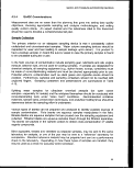 Methods
Table 4-10. Sample Preservation and Storage Parameters
Sample
Analyte
Nutrients
Ammonia
Nitrate
Nitrate + Nitrite
Nitrite
Total or dissolved metals
(except Hg)
Total or dissolved Hg
Particulate metals
Semivolatiles
Volatiles
Container3
P,G
P,G
P,G
P,G
P,G,TFEC
G.TFE
P,G
G
G
Size
500 mL
100mL
200 mL
100ml_
500mL
250 mL
1 gal
1 L
40 mL
Storage
Preservative
H2SO4, pH<2b
HaSCH, pH<2b
refrigerate
H2SO4, pH<2b
H2SO4, pH<2b
HNOs, pH<2
HNOs, pH<2
_d
Cool, 4°C
extraction
Cool, 4°C
Lifetime
28 days
48 hours
28 days
48 hours
6 months
28 days
6 months
7 days to
7 days
a P = linear polyethylene, G = borosilicate glass, TFE = tetrafluoroethylene.
b It is recommended that samples be analyzed as soon as possible.
0 If aliquot for Hg taken from this sample, cannot use linear polyethylene.
d Samples should be filtered as soon as possible and always within 24 hr.
Laboratory Analyses
Laboratory performance standards as measured by method QC protocols should be
used to evaluate and select appropriate analytical methods. Changes in selected
laboratory protocols should only be considered and/or approved if proposed procedures
meet or exceed established performance criteria.
64
image:
Methods
Table 4-10. Sample Preservation and Storage Parameters
Sample
Analyte
Nutrients
Ammonia
Nitrate
Nitrate + Nitrite
Nitrite
Total or dissolved metals
(except Hg)
Total or dissolved Hg
Particulate metals
Semivolatiles
Volatiles
Container3
P,G
P,G
P,G
P,G
P,G,TFEC
G.TFE
P,G
G
G
Size
500 mL
100mL
200 mL
100ml_
500mL
250 mL
1 gal
1 L
40 mL
Storage
Preservative
H2SO4, pH<2b
HaSCH, pH<2b
refrigerate
H2SO4, pH<2b
H2SO4, pH<2b
HNOs, pH<2
HNOs, pH<2
_d
Cool, 4°C
extraction
Cool, 4°C
Lifetime
28 days
48 hours
28 days
48 hours
6 months
28 days
6 months
7 days to
7 days
a P = linear polyethylene, G = borosilicate glass, TFE = tetrafluoroethylene.
b It is recommended that samples be analyzed as soon as possible.
0 If aliquot for Hg taken from this sample, cannot use linear polyethylene.
d Samples should be filtered as soon as possible and always within 24 hr.
Laboratory Analyses
Laboratory performance standards as measured by method QC protocols should be
used to evaluate and select appropriate analytical methods. Changes in selected
laboratory protocols should only be considered and/or approved if proposed procedures
meet or exceed established performance criteria.
64
image:
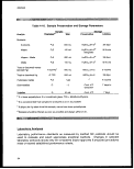 Section 403 Procedural and Monitoring Guidance
QA reports should describe the results of quantitative QC analyses, as well as other
elements critical to accurate interpretation of analytical results. It is recommended that
these reports be recorded and stored in a data base for future reference.
Trip blanks indicate whether any contamination occurred in the field or during shipping
of samples. Rinsate blanks are used to check for contamination due to inadequate
cleaning of field equipment.
Field splits, treated and identified as separate samples, may be sent to the same
laboratory for analysis or one sample may be sent to a "reference" laboratory for
comparison. Standard reference material may be placed in a sample container at the
time of collection and sent "blind" to the laboratory.
Calibration standards should be analyzed at the beginning of sample analysis and
should be verified at the end of each 12-hr shift during which analyses are performed..
The concentrations of calibration standards should bracket the expected sample
concentrations, or sample dilutions or sample handling modifications (i.e., reduced
sample size) will be required.
Analysis of method or reagent blanks should be conducted to demonstrate the absence
of contamination from sample handling in the laboratory. At least one method blank
must be included with each batch of samples and should constitute at least 5 percent of
all samples analyzed. All blanks should be free of detectable concentrations of the
target compounds, or steps should be taken to remove the source of contamination
before sample analysis proceeds.
Spike recovery analyses are required to assess method performance for the particular
sample matrix. Spike recoveries serve as an indication of analytical accuracy, whereas
analysis of standard reference materials (SRMs) can measure extraction efficiency.
Commonly recommended control limits include 75-125 percent recovery for spikes and
80-120 percent recovery for the analysis of SRMs.
Replicates must be analy2:ed to monitor the precision of laboratory analyses. A
minimum of 5 percent of the analyses should be laboratory replicates. Field duplicates
should also be collected where practical. Common control limits are ±20 relative
percent difference between duplicates.
Currently, no universally accepted convention for reporting detection limits of analytical
procedures exists. Table 4-11 lists definitions of various detection limits used by the
American Chemical Society's Committee on Environmental Improvement (CEI). The
IDL does not address possible blank contaminants or matrix interferences and is not a
good standard for complex environmental matrices. The LOD and LOQ account for
65
image:
Section 403 Procedural and Monitoring Guidance
QA reports should describe the results of quantitative QC analyses, as well as other
elements critical to accurate interpretation of analytical results. It is recommended that
these reports be recorded and stored in a data base for future reference.
Trip blanks indicate whether any contamination occurred in the field or during shipping
of samples. Rinsate blanks are used to check for contamination due to inadequate
cleaning of field equipment.
Field splits, treated and identified as separate samples, may be sent to the same
laboratory for analysis or one sample may be sent to a "reference" laboratory for
comparison. Standard reference material may be placed in a sample container at the
time of collection and sent "blind" to the laboratory.
Calibration standards should be analyzed at the beginning of sample analysis and
should be verified at the end of each 12-hr shift during which analyses are performed..
The concentrations of calibration standards should bracket the expected sample
concentrations, or sample dilutions or sample handling modifications (i.e., reduced
sample size) will be required.
Analysis of method or reagent blanks should be conducted to demonstrate the absence
of contamination from sample handling in the laboratory. At least one method blank
must be included with each batch of samples and should constitute at least 5 percent of
all samples analyzed. All blanks should be free of detectable concentrations of the
target compounds, or steps should be taken to remove the source of contamination
before sample analysis proceeds.
Spike recovery analyses are required to assess method performance for the particular
sample matrix. Spike recoveries serve as an indication of analytical accuracy, whereas
analysis of standard reference materials (SRMs) can measure extraction efficiency.
Commonly recommended control limits include 75-125 percent recovery for spikes and
80-120 percent recovery for the analysis of SRMs.
Replicates must be analy2:ed to monitor the precision of laboratory analyses. A
minimum of 5 percent of the analyses should be laboratory replicates. Field duplicates
should also be collected where practical. Common control limits are ±20 relative
percent difference between duplicates.
Currently, no universally accepted convention for reporting detection limits of analytical
procedures exists. Table 4-11 lists definitions of various detection limits used by the
American Chemical Society's Committee on Environmental Improvement (CEI). The
IDL does not address possible blank contaminants or matrix interferences and is not a
good standard for complex environmental matrices. The LOD and LOQ account for
65
image:
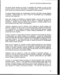 Methods
blanks, but not matrix interferences. The MDL provides high statistical confidence but,
like the LOQ, may be too stringent. Detection limits must be specified and reported to
ensure adequate data quality and comparability between protocols.
4.2.5 Statistical Design Considerations
The statistical analysis of water chemistry data typically involves calculating summary
statistics and testing for spatial and temporal trends. Summary conditions are useful for
spatial displays (e.g., plume contours), load estimations, and general reporting. Testing
for trends is useful for evaluating whether water chemistry conditions have improved or
degraded over time or space. In comparison to other variables (e.g., see
Bioaccumulation Methods), it is not common to collect replicated or composite data
except for QC procedures. This is the usual case since most monitoring designs
typically opt for collecting water chemistry data more frequently or at more stations.
Summary Statistics
To summarize data, the analyst typically estimates statistics for central tendency (e.g.,
mean, median) and variability (e.g., standard deviation, interquartile range) of grouped
data. Uncertainty should be indicated by reporting estimates with confidence limits or
Table 4-11. Definitions for Selected Limits of Detection
Instrument Detection Limit (IDL)
Limit of Detection (LOD)
Limit of Quantitation (LOQ)
Method Detection Limit (MDL)
The smallest signal above background noise that an
instrument can detect reliably.
The lowest concentration level that can be determined
to be statistically different from the blank. The
recommended value for LOD is 3a, where a is the
standard deviation of the blank in replicate analyses.
The level above which quantitative results may be
obtained with a specified degree of confidence. The
recommended value for LOQ is 10a, where a is the
standard deviation of the blank in replicate analyses.
The minimum concentration of a substance that can
be identified, measured, and reported with 99 percent
confidence that the analyte concentration is greater
than zero. The MDL is determined from seven
replicate analyses of a sample of a given matrix
containing the analyte.
66
image:
Methods
blanks, but not matrix interferences. The MDL provides high statistical confidence but,
like the LOQ, may be too stringent. Detection limits must be specified and reported to
ensure adequate data quality and comparability between protocols.
4.2.5 Statistical Design Considerations
The statistical analysis of water chemistry data typically involves calculating summary
statistics and testing for spatial and temporal trends. Summary conditions are useful for
spatial displays (e.g., plume contours), load estimations, and general reporting. Testing
for trends is useful for evaluating whether water chemistry conditions have improved or
degraded over time or space. In comparison to other variables (e.g., see
Bioaccumulation Methods), it is not common to collect replicated or composite data
except for QC procedures. This is the usual case since most monitoring designs
typically opt for collecting water chemistry data more frequently or at more stations.
Summary Statistics
To summarize data, the analyst typically estimates statistics for central tendency (e.g.,
mean, median) and variability (e.g., standard deviation, interquartile range) of grouped
data. Uncertainty should be indicated by reporting estimates with confidence limits or
Table 4-11. Definitions for Selected Limits of Detection
Instrument Detection Limit (IDL)
Limit of Detection (LOD)
Limit of Quantitation (LOQ)
Method Detection Limit (MDL)
The smallest signal above background noise that an
instrument can detect reliably.
The lowest concentration level that can be determined
to be statistically different from the blank. The
recommended value for LOD is 3a, where a is the
standard deviation of the blank in replicate analyses.
The level above which quantitative results may be
obtained with a specified degree of confidence. The
recommended value for LOQ is 10a, where a is the
standard deviation of the blank in replicate analyses.
The minimum concentration of a substance that can
be identified, measured, and reported with 99 percent
confidence that the analyte concentration is greater
than zero. The MDL is determined from seven
replicate analyses of a sample of a given matrix
containing the analyte.
66
image:
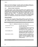 Section 403 Procedural and Monitoring Guidance
percentiles (Ward and Loftis, 1986). Alternatively, data may be summarized graphically
with plots (e.g., box and whisker plots, time series plots, scatter plots, contours, profiles,
etc.).
When developing summary statistics, it is important to use comparable data. It is
recommended that data collected or analyzed with different methods not be combined
unless a study comparing the different methods has been performed. An appropriate
study would establish the level of comparability between methods.
For the purposes of estimating summary statistics, it is generally recommended that
statistics not be used on left-censored data (i.e., data less than or equal to the detection
limit). Porter et al. (1988) and Gilliom and Helsel (1986) provide a discussion on the
implications of analyzing left-censored data and alternative procedures for estimating
summary statistics when the data are censored.
Trend Detection
Prior to the collection of data, the statistical test (and significance level) used to analyze
the data should be specified. By specifying the test to be used a priori, the monitoring
plan can be designed to ensure that the correct type of data (e.g., spatial versus
temporal coverage) is collected.
Monitoring programs can be evaluated using power analysis. The relative power of a
sampling is more meaningful when the relative costs of implementing alternative designs
are taken into consideration. Power-cost analyses are fundamental in selecting
appropriate sample/replicate number, sample location, and sampling frequency (Ferraro
etal.,1989).
For allocating samples and resources, Hirsch (1988) provides an approach for
evaluating alternative sampling strategies for two-sample designs. This approach would
be appropriate when comparing concentrations of a water chemistry variable from two
different locations (e.g., an impaired and control area) or two different time periods (e.g.,
two different cruises) at the same location. As a general recommendation, equal
resources (e.g., equal number of samples) should be allocated for each sampling period
for two-sample designs (Hirsch, 1988).
4.2.6
Use of Data
Results of the chemical analyses can be used to monitor levels of pollutants both in the
zone of initial dilution and in areas only minimally affected by the discharge. Sampling in
this manner establishes spatial trends in the accumulation and transport of discharged
pollutants.
67
image:
Section 403 Procedural and Monitoring Guidance
percentiles (Ward and Loftis, 1986). Alternatively, data may be summarized graphically
with plots (e.g., box and whisker plots, time series plots, scatter plots, contours, profiles,
etc.).
When developing summary statistics, it is important to use comparable data. It is
recommended that data collected or analyzed with different methods not be combined
unless a study comparing the different methods has been performed. An appropriate
study would establish the level of comparability between methods.
For the purposes of estimating summary statistics, it is generally recommended that
statistics not be used on left-censored data (i.e., data less than or equal to the detection
limit). Porter et al. (1988) and Gilliom and Helsel (1986) provide a discussion on the
implications of analyzing left-censored data and alternative procedures for estimating
summary statistics when the data are censored.
Trend Detection
Prior to the collection of data, the statistical test (and significance level) used to analyze
the data should be specified. By specifying the test to be used a priori, the monitoring
plan can be designed to ensure that the correct type of data (e.g., spatial versus
temporal coverage) is collected.
Monitoring programs can be evaluated using power analysis. The relative power of a
sampling is more meaningful when the relative costs of implementing alternative designs
are taken into consideration. Power-cost analyses are fundamental in selecting
appropriate sample/replicate number, sample location, and sampling frequency (Ferraro
etal.,1989).
For allocating samples and resources, Hirsch (1988) provides an approach for
evaluating alternative sampling strategies for two-sample designs. This approach would
be appropriate when comparing concentrations of a water chemistry variable from two
different locations (e.g., an impaired and control area) or two different time periods (e.g.,
two different cruises) at the same location. As a general recommendation, equal
resources (e.g., equal number of samples) should be allocated for each sampling period
for two-sample designs (Hirsch, 1988).
4.2.6
Use of Data
Results of the chemical analyses can be used to monitor levels of pollutants both in the
zone of initial dilution and in areas only minimally affected by the discharge. Sampling in
this manner establishes spatial trends in the accumulation and transport of discharged
pollutants.
67
image:
 Methods
The data can also be used as boundary and initial conditions for modeling work that may
be used to map the transport and fate of various chemicals throughout the ecosystem
under varying discharge scenarios. The modeling can lead to developing water quality
standards and discharge guidelines. During the monitoring program, water chemistry
data can be used to identify discharges that are not in compliance and to ensure that
water quality standards are being maintained.
Monitoring of pollutant levels in the water column is a widely-accepted means of
measuring the condition of the aquatic habitat. However, the singular use of pollutant
loading data to assess the condition of the water column or to guide the decision-making
process is not recommended. Data acquired from monitoring water contaminant levels,
in conjunction with the water's physical properties, may be used to assess the health
risks to human populations and the ecological risks to individuals, populations, and
communities living in the water column. Monitoring of water column chemistry remains
a powerful tool in the evaluation of spatial and temporal effects of anthropogenic and
natural disturbance.
4.2.7 Summary and Recommendations
Rationale
• Monitoring water quality parameters will provide information on ambient water
conditions and the potential for transport and persistence of contaminants
from permitted discharges.
Monitoring Design Considerations
• The analytical methods must show appropriate selectivity, specificity, and
sensitivity for the contaminants of concern.
• Sampling and sample-handling procedures should be well-defined and
consistent so as not to compromise the integrity and representativeness of
the samples.
• Sampling numbers and locations should be appropriate to the level of
information required.
Analytical Methods Considerations
• The Winkler (titrimetric) method is the first method of choice for the
measurement of dissolved oxygen unless the samples contain interferents
such as sulfur compounds, chlorine, free iodine, color, turbidity, or biological
floes, or when continuous monitoring is planned. In those instances, a
membrane electrode should be used.
68
image:
Methods
The data can also be used as boundary and initial conditions for modeling work that may
be used to map the transport and fate of various chemicals throughout the ecosystem
under varying discharge scenarios. The modeling can lead to developing water quality
standards and discharge guidelines. During the monitoring program, water chemistry
data can be used to identify discharges that are not in compliance and to ensure that
water quality standards are being maintained.
Monitoring of pollutant levels in the water column is a widely-accepted means of
measuring the condition of the aquatic habitat. However, the singular use of pollutant
loading data to assess the condition of the water column or to guide the decision-making
process is not recommended. Data acquired from monitoring water contaminant levels,
in conjunction with the water's physical properties, may be used to assess the health
risks to human populations and the ecological risks to individuals, populations, and
communities living in the water column. Monitoring of water column chemistry remains
a powerful tool in the evaluation of spatial and temporal effects of anthropogenic and
natural disturbance.
4.2.7 Summary and Recommendations
Rationale
• Monitoring water quality parameters will provide information on ambient water
conditions and the potential for transport and persistence of contaminants
from permitted discharges.
Monitoring Design Considerations
• The analytical methods must show appropriate selectivity, specificity, and
sensitivity for the contaminants of concern.
• Sampling and sample-handling procedures should be well-defined and
consistent so as not to compromise the integrity and representativeness of
the samples.
• Sampling numbers and locations should be appropriate to the level of
information required.
Analytical Methods Considerations
• The Winkler (titrimetric) method is the first method of choice for the
measurement of dissolved oxygen unless the samples contain interferents
such as sulfur compounds, chlorine, free iodine, color, turbidity, or biological
floes, or when continuous monitoring is planned. In those instances, a
membrane electrode should be used.
68
image:
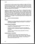 Section 403 Procedural and Monitoring Quittance
• Nutrients such as ammonia nitrogen, total Kjeldahl nitrogen, nitrate-nitrite
nitrogen, and phosphorus are determined by spectrophotometric
measurements using a segmented continuous flow analyzer.
• The usual method for chlorophyll determination is fluorometric; however, the
choice of method is determined by the need to separate the different forms.
HPLC is the most accurate method, but it is also the most expensive.
• A combination of AA spectroscopy and ICP spectrometry is the
recommended method for the detection of metals.
• Cold vapor AA spectroscopy is the recommended protocol for the detection of
mercury.
• For monitoring programs where the most accurate quantitation is important,
the isotope dilution GC/MS method is recommended for volatile and
semivolatile organic compounds. GC/ECD is the method of choice for many
organic chemicals (e.g., pesticides and RGBs).
QA/QC Considerations
• Calibration standards and blank, matrix spike, and replicate analyses are
recommended quality control checks.
• A report describing the objectives of the analytical effort; methods of sample
collection, handling, and preservation; details of the analytical method;
problems encountered during the analytical process; any necessary
modifications to the written procedures; and results of the QC analyses
should be included with the quantitative data.
Statistical Design Considerations
• The analyst typically estimates statistics for central tendency (e.g., mean,
median) and variability (e.g., standard deviation, interquartile range) of
grouped data. Uncertainty should be indicated by reporting estimates with
confidence limits or percehtiles.
• When developing summary statistics, it is important to use comparable data.
It is recommended that data collected or analyzed with different methods not
be combined unless a study comparing the different methods has been
performed.
• For the purpose of estimating summary statistics, it is generally
recommended that statistics not be performed on left-censored data.
• Prior to the collection of data, the statistical test (and significance level) used
to analyze the data should be specified.
69
image:
Section 403 Procedural and Monitoring Quittance
• Nutrients such as ammonia nitrogen, total Kjeldahl nitrogen, nitrate-nitrite
nitrogen, and phosphorus are determined by spectrophotometric
measurements using a segmented continuous flow analyzer.
• The usual method for chlorophyll determination is fluorometric; however, the
choice of method is determined by the need to separate the different forms.
HPLC is the most accurate method, but it is also the most expensive.
• A combination of AA spectroscopy and ICP spectrometry is the
recommended method for the detection of metals.
• Cold vapor AA spectroscopy is the recommended protocol for the detection of
mercury.
• For monitoring programs where the most accurate quantitation is important,
the isotope dilution GC/MS method is recommended for volatile and
semivolatile organic compounds. GC/ECD is the method of choice for many
organic chemicals (e.g., pesticides and RGBs).
QA/QC Considerations
• Calibration standards and blank, matrix spike, and replicate analyses are
recommended quality control checks.
• A report describing the objectives of the analytical effort; methods of sample
collection, handling, and preservation; details of the analytical method;
problems encountered during the analytical process; any necessary
modifications to the written procedures; and results of the QC analyses
should be included with the quantitative data.
Statistical Design Considerations
• The analyst typically estimates statistics for central tendency (e.g., mean,
median) and variability (e.g., standard deviation, interquartile range) of
grouped data. Uncertainty should be indicated by reporting estimates with
confidence limits or percehtiles.
• When developing summary statistics, it is important to use comparable data.
It is recommended that data collected or analyzed with different methods not
be combined unless a study comparing the different methods has been
performed.
• For the purpose of estimating summary statistics, it is generally
recommended that statistics not be performed on left-censored data.
• Prior to the collection of data, the statistical test (and significance level) used
to analyze the data should be specified.
69
image:
 Methods
• Monitoring programs can be evaluated using power analysis for detecting
long-term (monotonic) trends in nutrient data. In general, the approach
described there can be applied for other variables and statistical tests (e.g.,
monotonic or step-trend test).
Use of Data
• Monitor ambient levels of pollutants in the environment.
• Establish spatial and temporal trends in the accumulation and transport of
pollutants discharged into ambient waters.
• Calibrate and verify mathematical models.
• Develop water quality standards for receiving waters.
• Identify noncompliant discharges.
70
image:
Methods
• Monitoring programs can be evaluated using power analysis for detecting
long-term (monotonic) trends in nutrient data. In general, the approach
described there can be applied for other variables and statistical tests (e.g.,
monotonic or step-trend test).
Use of Data
• Monitor ambient levels of pollutants in the environment.
• Establish spatial and temporal trends in the accumulation and transport of
pollutants discharged into ambient waters.
• Calibrate and verify mathematical models.
• Develop water quality standards for receiving waters.
• Identify noncompliant discharges.
70
image:
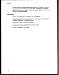 Section 403 Procedural and Monitoring Guidance
4.3
SEDIMENT CHEMISTRY
Monitoring of pollutant levels in sediments is a widely-accepted means of measuring the
condition of the benthic habitat and is a powerful tool in the evaluation of spatial and
temporal effects of anthropogenic and natural disturbance. Sediment pollutant loading
data should be used, however, in conjunction with other tools to assess the condition of
the benthic habitat or to guide the decision-making process.
4.3.1
Rationale
Of the 10 guidelines used to determine unreasonable degradation or irreparable harm,
the following can be assessed by evaluating sediment chemistry:
• Quantities, composition, and potential bioaccumulation or persistence of the
pollutants to be discharged;
• Potential transport of the pollutants by biological, physical, or chemical
processes; and
• Potential direct or indirect impacts on human health.
The sediments represent a potential sink for many chemical contaminants in the marine
environment (USEPA, 1989e). The objective of monitoring bulk sediment chemistry is to
detect sediment toxicity and to describe spatial and temporal changes in sediment
pollutants. The results may be used to monitor rates of change following discharge
initialization, to evaluate the condition of benthic habitats, and to provide early warnings
of potential impacts to the marine ecosystem.
4.3.2 Monitoring Design Considerations
Selection of Analytes
The chemicals that should be included in the monitoring program are those chemicals
known or suspected to be in the discharge, as well as possible by-products. Although
potentially toxic compounds in the discharge may not be fully known, the objectives of
the program must be clearly defined. It may be necessary at the beginning of the
program to conduct an analysis for all chemicals on the EPA-defined Priority Pollutant,
Hazardous Substance, or Target Compound/Analyte Lists to determine which are
present; however, detection in the environment does not always correlate with biological
risks and effects. Limitations in analytical methodology, modeling techniques, and
toxicological data restrict the usefulness of the resulting data. In some cases, levels of
contaminants that are of concern to the health of organisms are below the lowest limit of
detection of the best available analytical methodology.
71
image:
Section 403 Procedural and Monitoring Guidance
4.3
SEDIMENT CHEMISTRY
Monitoring of pollutant levels in sediments is a widely-accepted means of measuring the
condition of the benthic habitat and is a powerful tool in the evaluation of spatial and
temporal effects of anthropogenic and natural disturbance. Sediment pollutant loading
data should be used, however, in conjunction with other tools to assess the condition of
the benthic habitat or to guide the decision-making process.
4.3.1
Rationale
Of the 10 guidelines used to determine unreasonable degradation or irreparable harm,
the following can be assessed by evaluating sediment chemistry:
• Quantities, composition, and potential bioaccumulation or persistence of the
pollutants to be discharged;
• Potential transport of the pollutants by biological, physical, or chemical
processes; and
• Potential direct or indirect impacts on human health.
The sediments represent a potential sink for many chemical contaminants in the marine
environment (USEPA, 1989e). The objective of monitoring bulk sediment chemistry is to
detect sediment toxicity and to describe spatial and temporal changes in sediment
pollutants. The results may be used to monitor rates of change following discharge
initialization, to evaluate the condition of benthic habitats, and to provide early warnings
of potential impacts to the marine ecosystem.
4.3.2 Monitoring Design Considerations
Selection of Analytes
The chemicals that should be included in the monitoring program are those chemicals
known or suspected to be in the discharge, as well as possible by-products. Although
potentially toxic compounds in the discharge may not be fully known, the objectives of
the program must be clearly defined. It may be necessary at the beginning of the
program to conduct an analysis for all chemicals on the EPA-defined Priority Pollutant,
Hazardous Substance, or Target Compound/Analyte Lists to determine which are
present; however, detection in the environment does not always correlate with biological
risks and effects. Limitations in analytical methodology, modeling techniques, and
toxicological data restrict the usefulness of the resulting data. In some cases, levels of
contaminants that are of concern to the health of organisms are below the lowest limit of
detection of the best available analytical methodology.
71
image:
 Methods
Sampling Considerations
Selection of sampling locations and choice of sampling techniques are crucial decisions
to be made before the sampling effort is initiated. Recommended Protocols for
Measuring Selected Environmental Variables in Puget Sound (USEPA, 1986-1991)
contains discussions of quality assurance requirements and sampling considerations
that are applicable to sediment quality monitoring. Sampling must incorporate sites
within the zone of initial dilution, extending out to areas of low contaminant concentration
and further to unaffected areas to obtain the complete spatial variability. A summary of
sample containers and handling guidelines is presented in Table 4-12.
Sediment Sampling Devices
The protocols required to collect an acceptable surficial sediment sample for subsequent
measurement of chemical variables have generally been neglected. In fact, sampling
crews have been given wide latitude in how samples are collected. Because sample
collection protocols influence all subsequent laboratory and data analysis, however, it is
essential that sediment samples be collected using acceptable and standardized
techniques. Sediment sampling devices are the same regardless of whether the
samples are collected for chemistry, grain size, or benthic infauna analyses.
Consequently, enough sediment may be collected in the same grab or core for all three
analyses. Equipment selection depends in large part on the use of the sample
collected. Consideration should also be given to water depth, currents, ocean bottom
characteristics, and degree of homogeneity and representativeness of sampling.
Collection of undisturbed sediment requires that the sampler:
• Create a minimal bow wake when descending;
• Form a leakproof seal when the sediment sample is taken;
• Prevent winnowing and excessive sample disturbance when ascending; and
• Allow easy access to the sample surface in order that undisturbed
subsamples may be taken (ASTM, 1991).
Penetration well below the desired sampling depth is preferred to prevent sample
disturbance as the device closes. It is best to use a sampler with a weight adjustment to
enable the modification of penetration depths.
Several types of devices can be used to collect sediment samples: dredges, grabs, and
box corers (Mclntyre et al., 1984). There are many variations to these types of sampling
device. Many of these devices sample the benthic habitat in a unique manner (Table
4-13). Accordingly, conducting comparisons between data collected using different
devices is inadvisable.
72
image:
Methods
Sampling Considerations
Selection of sampling locations and choice of sampling techniques are crucial decisions
to be made before the sampling effort is initiated. Recommended Protocols for
Measuring Selected Environmental Variables in Puget Sound (USEPA, 1986-1991)
contains discussions of quality assurance requirements and sampling considerations
that are applicable to sediment quality monitoring. Sampling must incorporate sites
within the zone of initial dilution, extending out to areas of low contaminant concentration
and further to unaffected areas to obtain the complete spatial variability. A summary of
sample containers and handling guidelines is presented in Table 4-12.
Sediment Sampling Devices
The protocols required to collect an acceptable surficial sediment sample for subsequent
measurement of chemical variables have generally been neglected. In fact, sampling
crews have been given wide latitude in how samples are collected. Because sample
collection protocols influence all subsequent laboratory and data analysis, however, it is
essential that sediment samples be collected using acceptable and standardized
techniques. Sediment sampling devices are the same regardless of whether the
samples are collected for chemistry, grain size, or benthic infauna analyses.
Consequently, enough sediment may be collected in the same grab or core for all three
analyses. Equipment selection depends in large part on the use of the sample
collected. Consideration should also be given to water depth, currents, ocean bottom
characteristics, and degree of homogeneity and representativeness of sampling.
Collection of undisturbed sediment requires that the sampler:
• Create a minimal bow wake when descending;
• Form a leakproof seal when the sediment sample is taken;
• Prevent winnowing and excessive sample disturbance when ascending; and
• Allow easy access to the sample surface in order that undisturbed
subsamples may be taken (ASTM, 1991).
Penetration well below the desired sampling depth is preferred to prevent sample
disturbance as the device closes. It is best to use a sampler with a weight adjustment to
enable the modification of penetration depths.
Several types of devices can be used to collect sediment samples: dredges, grabs, and
box corers (Mclntyre et al., 1984). There are many variations to these types of sampling
device. Many of these devices sample the benthic habitat in a unique manner (Table
4-13). Accordingly, conducting comparisons between data collected using different
devices is inadvisable.
72
image:
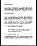 Section 403 Procedural and Monitoring Guidance
Table 4-12. Sampling Containers, Preservation Requirements, and Holding
Times for Sediment Samples
Container3
Contaminant
Acidity
Alkalinity
Ammonia
Sulfate
Sulfide
Sulfite
Nitrate
Nitrate-nitrite
Nitrite
Oil and grease
Organic carbon
Metals
Chromium VI
Mercury
Metals, except above
Organic Compounds
Extractables (including phthalates, G, Teflon-lined cap
nitrosamines, organochlorine pesticides,
PCBs, nitroaromatics, isophorone,
polynuclear aromatic hydrocarbons,
haloethers, chlorinated hydrocarbons,
and TCDD)
Extractables (phenols)
Purgeables (halocarbons and aromatics)
Purgeables (arolein and acrylonitrite)
Orthophosphate
Pesticides
Phenols
Phosphorus (elemental)
Phosphorus, total
Chlorinated organic compounds
G, teflon-lined cap
G, Teflon-lined
septum
G, Teflon-lined
septum
P,G
G, Teflon-lined cap
P,G
G
P,G
G, Teflon-lined cap
Preservation Holding Time
P,G
P,G
P,G
P,G
P,G
P,G
P,G
P.G
P,G
G
P,G
P,G
P,G
P,G
Cool, 4°C
Cool, 4°C
Cool, 4°C
Cool, 4°C
Cool, 4°C
Cool, 4°C
Cool, 4°C
Cool, 4°C
Cool, 4°C
Cool, 4°C
Cool, 4°C
Cool, 4°C
14 days
14 days
28 days
28 days
28 days
48 hours
48 hours
28 days
48 hours
28 days
28 days
48 hours
28 days
180 days
Cool, 4°C
7 days (until extraction)
40 days (after extraction)
Cool, 4°C
Cool, 4°C
Cool, 4°C
Cool, 4°C
Cool, 4°C
Cool, 4°C
Cool, 4°C
Cool, 4°C
Cool, 4°C
7 days (until extraction)
40 days (after extraction)
7 days
3 days
48 hours
7 days (until extraction)
40 days (after extraction)
28 days
48 hours
28 days
7 days (until extraction)
30 days (after extraction)
aPolyethylene (P) or glass (G)
SOURCE: ASTM, 1991.
73
image:
Section 403 Procedural and Monitoring Guidance
Table 4-12. Sampling Containers, Preservation Requirements, and Holding
Times for Sediment Samples
Container3
Contaminant
Acidity
Alkalinity
Ammonia
Sulfate
Sulfide
Sulfite
Nitrate
Nitrate-nitrite
Nitrite
Oil and grease
Organic carbon
Metals
Chromium VI
Mercury
Metals, except above
Organic Compounds
Extractables (including phthalates, G, Teflon-lined cap
nitrosamines, organochlorine pesticides,
PCBs, nitroaromatics, isophorone,
polynuclear aromatic hydrocarbons,
haloethers, chlorinated hydrocarbons,
and TCDD)
Extractables (phenols)
Purgeables (halocarbons and aromatics)
Purgeables (arolein and acrylonitrite)
Orthophosphate
Pesticides
Phenols
Phosphorus (elemental)
Phosphorus, total
Chlorinated organic compounds
G, teflon-lined cap
G, Teflon-lined
septum
G, Teflon-lined
septum
P,G
G, Teflon-lined cap
P,G
G
P,G
G, Teflon-lined cap
Preservation Holding Time
P,G
P,G
P,G
P,G
P,G
P,G
P,G
P.G
P,G
G
P,G
P,G
P,G
P,G
Cool, 4°C
Cool, 4°C
Cool, 4°C
Cool, 4°C
Cool, 4°C
Cool, 4°C
Cool, 4°C
Cool, 4°C
Cool, 4°C
Cool, 4°C
Cool, 4°C
Cool, 4°C
14 days
14 days
28 days
28 days
28 days
48 hours
48 hours
28 days
48 hours
28 days
28 days
48 hours
28 days
180 days
Cool, 4°C
7 days (until extraction)
40 days (after extraction)
Cool, 4°C
Cool, 4°C
Cool, 4°C
Cool, 4°C
Cool, 4°C
Cool, 4°C
Cool, 4°C
Cool, 4°C
Cool, 4°C
7 days (until extraction)
40 days (after extraction)
7 days
3 days
48 hours
7 days (until extraction)
40 days (after extraction)
28 days
48 hours
28 days
7 days (until extraction)
30 days (after extraction)
aPolyethylene (P) or glass (G)
SOURCE: ASTM, 1991.
73
image:
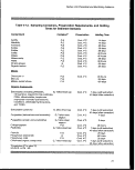 Methods
Table 4-13. Summary of Bottom Sampling Equipment8
Device
Use
Advantages
Disadvantages
Fluorocarfaon plastic
or glass
tubs
Shallow wadable waters
or deep waters if
SCUBA available. Soft
or semiconsolidated
deposits.
Preserves layering and
permits historical sudy of
sediment deposition.
Rapid-samples immed-
iately ready for laboratory
shipment. Minimal risk of
contamination.
Small sample size requires
repetitive sampling.
Hand oorer with
removable
fluorocarbon plastic
or glass liners
Same as above except
more consolidated sedi-
ments can be obtained.
Handles provide for greater
ease of substrate
penetration. Above
advantages.
Careful handling necessary to
prevent spillage, Requires
removal of liners before repetitive
sampling. Slight risk of metal
contamination from barrel and
core cutter.
Box corer
Gravity corers, that
is, Phleger corer
Young grab (fluoro-
carbon plastic- or
Kynar-lined modi-
fied 0.1m2 Van
Veen)
Ekman or box
dredge
Same as above.
Semiconsolidated
sediments.
Collection of large
undisturbed sample
allowing for subsampling.
Low risk of undisturbed
sample contamination.
Maintains sediment •
integrity relatively well.
Lakes and marine areas. Eliminates metal
contamination. Reduces
pressure wave.
Soft to semisoft
sediments. Can be
used from boat, bridge,
or pier in waters of
various depths.
Obtains a larger sample
than coring tubes. Can be
subsampled through box
lid.
Hard to handle.
Careful handling necessary to
avoid sediment spillage. Small
sample, requires repetitive
operation and removal of liners.
Time-consuming.
Expensive. Requires winch.
Possible incomplete jaw closure
and sample loss. Possible shock
wave, which may disturb the fine
sediments ("fines"). Metal
construction may introduce
contaminants. Possible loss of
"fines" on retrieval.
Ponar grab
sampler
Useful on sand, silt,
or clay.
Most universal grab
sampler. Adequate on most
substrates. Large sample
obtained intact, permitting
subsampling.
Shock wave from descent may
disturb "fines." Possible
incomplete closure of jaws results
in sample loss. Possible
contamination from metal frame
construction. Sample must be
further prepared for analysis.
74
image:
Methods
Table 4-13. Summary of Bottom Sampling Equipment8
Device
Use
Advantages
Disadvantages
Fluorocarfaon plastic
or glass
tubs
Shallow wadable waters
or deep waters if
SCUBA available. Soft
or semiconsolidated
deposits.
Preserves layering and
permits historical sudy of
sediment deposition.
Rapid-samples immed-
iately ready for laboratory
shipment. Minimal risk of
contamination.
Small sample size requires
repetitive sampling.
Hand oorer with
removable
fluorocarbon plastic
or glass liners
Same as above except
more consolidated sedi-
ments can be obtained.
Handles provide for greater
ease of substrate
penetration. Above
advantages.
Careful handling necessary to
prevent spillage, Requires
removal of liners before repetitive
sampling. Slight risk of metal
contamination from barrel and
core cutter.
Box corer
Gravity corers, that
is, Phleger corer
Young grab (fluoro-
carbon plastic- or
Kynar-lined modi-
fied 0.1m2 Van
Veen)
Ekman or box
dredge
Same as above.
Semiconsolidated
sediments.
Collection of large
undisturbed sample
allowing for subsampling.
Low risk of undisturbed
sample contamination.
Maintains sediment •
integrity relatively well.
Lakes and marine areas. Eliminates metal
contamination. Reduces
pressure wave.
Soft to semisoft
sediments. Can be
used from boat, bridge,
or pier in waters of
various depths.
Obtains a larger sample
than coring tubes. Can be
subsampled through box
lid.
Hard to handle.
Careful handling necessary to
avoid sediment spillage. Small
sample, requires repetitive
operation and removal of liners.
Time-consuming.
Expensive. Requires winch.
Possible incomplete jaw closure
and sample loss. Possible shock
wave, which may disturb the fine
sediments ("fines"). Metal
construction may introduce
contaminants. Possible loss of
"fines" on retrieval.
Ponar grab
sampler
Useful on sand, silt,
or clay.
Most universal grab
sampler. Adequate on most
substrates. Large sample
obtained intact, permitting
subsampling.
Shock wave from descent may
disturb "fines." Possible
incomplete closure of jaws results
in sample loss. Possible
contamination from metal frame
construction. Sample must be
further prepared for analysis.
74
image:
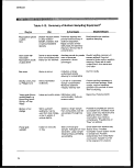 Section 403 Procedural and Monitoring Guidance
Table 4-13. (continued)
Device
Use
Advantages
Disadvantages
BMH-53 piston
corer
Waters of 4-6 ft depth
when used with
extension rod. Soft to
semiconsolidated
deposits.
Piston provides for greater
sample retention.
Cores must be extruded on site to
other containers. Metal barrels
introduce risk of metal
contamination.
Van Veen
BMH-60
Useful on sand, silt, or
clay.
Sampling moving
waters from a fixed
platform.
Adequate on most
substrates. Large sample
obtained intact, permitting
subsampling.
Streamlined configuration
allows sampling where
other devices could not
achieve proper orien-
tiation.
Shock wave from descent may
disturb "fines." Possible
incomplete closure of jaws results
in sample loss. Possible
contamination from metal frame
construction. Sample must be
further prepared for analysis.
Possible contamination from
metal construction. Subsampling
difficult. Not effective for sampling
fine sediments.
Petersen grab
sampler
Shipek grab
sampler
Orange-peel grab
Smith-Mclntyre
grab
Useful on most
substrates.
Used primarily in
marine waters and large
inland lakes and
reservoirs.
Useful on most
substrates.
Scoops, drag buckets Various environments
depending on depth
and substrate.
Large sample; can
penetrate most substrates.
Sample bucket may be
opened to permit
subsampling. Retains
fine-grained sediments
effectively.
Designed for sampling hard
substrates.
Heavy, may require winch. No
cover lid to permit subsampling.
All other disadvantages of Ekman
and Ponar.
Possible contamination from
metal construction. Heavy, may
require winch.
Inexpensive, easy to
handle.
Loss of "fines." Heavy, may
require winch. Possible metal
contamination.
Loss of "fines" on retrieval
through water column.
aComments represent subjective evaluations.
SOURCE: ASTM, 1991.
75
image:
Section 403 Procedural and Monitoring Guidance
Table 4-13. (continued)
Device
Use
Advantages
Disadvantages
BMH-53 piston
corer
Waters of 4-6 ft depth
when used with
extension rod. Soft to
semiconsolidated
deposits.
Piston provides for greater
sample retention.
Cores must be extruded on site to
other containers. Metal barrels
introduce risk of metal
contamination.
Van Veen
BMH-60
Useful on sand, silt, or
clay.
Sampling moving
waters from a fixed
platform.
Adequate on most
substrates. Large sample
obtained intact, permitting
subsampling.
Streamlined configuration
allows sampling where
other devices could not
achieve proper orien-
tiation.
Shock wave from descent may
disturb "fines." Possible
incomplete closure of jaws results
in sample loss. Possible
contamination from metal frame
construction. Sample must be
further prepared for analysis.
Possible contamination from
metal construction. Subsampling
difficult. Not effective for sampling
fine sediments.
Petersen grab
sampler
Shipek grab
sampler
Orange-peel grab
Smith-Mclntyre
grab
Useful on most
substrates.
Used primarily in
marine waters and large
inland lakes and
reservoirs.
Useful on most
substrates.
Scoops, drag buckets Various environments
depending on depth
and substrate.
Large sample; can
penetrate most substrates.
Sample bucket may be
opened to permit
subsampling. Retains
fine-grained sediments
effectively.
Designed for sampling hard
substrates.
Heavy, may require winch. No
cover lid to permit subsampling.
All other disadvantages of Ekman
and Ponar.
Possible contamination from
metal construction. Heavy, may
require winch.
Inexpensive, easy to
handle.
Loss of "fines." Heavy, may
require winch. Possible metal
contamination.
Loss of "fines" on retrieval
through water column.
aComments represent subjective evaluations.
SOURCE: ASTM, 1991.
75
image:
 Methods
Grab samplers
Grabs are capable of consistent sampling of bottom habitats. Depending on the size of
the device, areas from 0.02 to 0.5 m2 and depths ranging from 5 to 15 cm may be
sampled. Limitations of grab samplers include :
• Variability among samples in penetration depth depending on sediment
properties;
• Oblique angles of penetration, which result in varying penetration depths
within a sample; and
• Folding of the sample, which results in the inability to section the sample and
the loss of information concerning the vertical structure in the sediments.
The careful use of these devices, however, will provide quantitative data. Grab
samplers are the tools of choice for a number of marine monitoring programs (Fredette
etal., 1989; USEPA, 1986-1991).
Core samplers
Box corers use a surrounding frame to ensure vertical entry; therefore, vertical
sectioning of the sample is possible (USEPA, 1986-1991). These devices are capable
of maximum penetration depths of 15 cm and may collect volumes 5 to 10 times those
of grab samplers. Limitations of box corers include :
• Large size and weight, which require the use of cranes or winches and a
large vessel for deployment;
• Higher construction expenses; and
• Lack of calibration studies to permit comparisons to grab samples.
The Hessler-Sandia box corer uses dividers to section the core into subsections,
facilitating subsampling of the core. Box corers are recognized as the tools of choice for
maximum accuracy and precision when sampling soft-bottom habitats.
Collection of sediments and collection of benthic organisms should be done concurrently
to mitigate the costs of field sampling and to permit sound correlation, regression, and
multivariate analyses. Therefore, it is recommended that the sampling device also be
suitable for benthic sampling. Grab and core sampling devices permit adequate
sampling of both sediment and benthic infaunal communities with one sampling device.
76
image:
Methods
Grab samplers
Grabs are capable of consistent sampling of bottom habitats. Depending on the size of
the device, areas from 0.02 to 0.5 m2 and depths ranging from 5 to 15 cm may be
sampled. Limitations of grab samplers include :
• Variability among samples in penetration depth depending on sediment
properties;
• Oblique angles of penetration, which result in varying penetration depths
within a sample; and
• Folding of the sample, which results in the inability to section the sample and
the loss of information concerning the vertical structure in the sediments.
The careful use of these devices, however, will provide quantitative data. Grab
samplers are the tools of choice for a number of marine monitoring programs (Fredette
etal., 1989; USEPA, 1986-1991).
Core samplers
Box corers use a surrounding frame to ensure vertical entry; therefore, vertical
sectioning of the sample is possible (USEPA, 1986-1991). These devices are capable
of maximum penetration depths of 15 cm and may collect volumes 5 to 10 times those
of grab samplers. Limitations of box corers include :
• Large size and weight, which require the use of cranes or winches and a
large vessel for deployment;
• Higher construction expenses; and
• Lack of calibration studies to permit comparisons to grab samples.
The Hessler-Sandia box corer uses dividers to section the core into subsections,
facilitating subsampling of the core. Box corers are recognized as the tools of choice for
maximum accuracy and precision when sampling soft-bottom habitats.
Collection of sediments and collection of benthic organisms should be done concurrently
to mitigate the costs of field sampling and to permit sound correlation, regression, and
multivariate analyses. Therefore, it is recommended that the sampling device also be
suitable for benthic sampling. Grab and core sampling devices permit adequate
sampling of both sediment and benthic infaunal communities with one sampling device.
76
image:
 Section 403 Procedural and Monitoring Guidance
Sample Depth
It is recommended that the upper 2 cm of the sediment column be examined to
characterize surficial sediments. Although the 2 cm specification is arbitrary, it does
ensure that relatively recent sediments are sampled, that adequate volumes of
sediments are readily obtained for laboratory analyses, and that data from different
studies can be compared.
Sampling of depths other than 2 cm or vertical stratification of deeper sediment cores
may be appropriate, depending on the objectives of the monitoring program and the rate
of sediment accumulation. For example, if information concerning only the most recent
sediment contamination is required, examination of the upper 1 cm may be appropriate.
Stratification of deeper cores will provide historical data of sediment contaminant levels
and depositional events. Comparison of data from studies analyzing different sediment
depths is not advised. If the potential for bioaccumulation of contaminants in infaunal
organisms is a concern, sampling to the depth of the anoxic layer is desirable.
Penetration well below the desired sampling depth is preferred to prevent sample
disturbance as the device closes.
Total Organic Carbon and Acid Volatile Sulfides Normalization
Total organic carbon (TOG) and acid volatile sulfides (AVS) are considered by many to
be the most important parameters in defining organic and metal concentrations in
sediments. Toxic hydrophobic contaminant concentrations have been found to be
related to the TOG content of the sediment (Karickhoff et al., 1979). Likewise, toxic
metals concentrations have been found to be related to the AVS concentration of the
sediment (DiToro et al., in press a, b). The AVS pool is available to bind metals, thereby
reducing their bioavailability.
Normalizations of sediment contaminant concentrations to TOG and AVS have been
conducted to estimate the bioavailability of inorganic and organic contaminants.
Furthermore, these normalizations have been made to account for some of the
variability found in bioaccumulation rates and biological assemblages. TOC/lipid
normalized accumulation factors (AF) have also been used to predict tissue residue
concentrations (Ferraro et al., 1990; Lake et al., 1987). AVS will be used in a similar
manner to assist in the development of accumulation factors for metals.
Normalization based on AVS concentrations is considered a potentially useful tool for
assessing the bioavailability of certain divalent metals (e.g., Cd and Ni). However, only
a few laboratories can perform these analyses at present and the procedure has not
undergone any round robin verification. In addition, sampling for AVS is very subject to
error because contact with air can greatly affect results. Although AVS normalizations
represent a promising tool for evaluation of sediment metals data, general use in
estuarine monitoring programs may not yet be practical.
77
image:
Section 403 Procedural and Monitoring Guidance
Sample Depth
It is recommended that the upper 2 cm of the sediment column be examined to
characterize surficial sediments. Although the 2 cm specification is arbitrary, it does
ensure that relatively recent sediments are sampled, that adequate volumes of
sediments are readily obtained for laboratory analyses, and that data from different
studies can be compared.
Sampling of depths other than 2 cm or vertical stratification of deeper sediment cores
may be appropriate, depending on the objectives of the monitoring program and the rate
of sediment accumulation. For example, if information concerning only the most recent
sediment contamination is required, examination of the upper 1 cm may be appropriate.
Stratification of deeper cores will provide historical data of sediment contaminant levels
and depositional events. Comparison of data from studies analyzing different sediment
depths is not advised. If the potential for bioaccumulation of contaminants in infaunal
organisms is a concern, sampling to the depth of the anoxic layer is desirable.
Penetration well below the desired sampling depth is preferred to prevent sample
disturbance as the device closes.
Total Organic Carbon and Acid Volatile Sulfides Normalization
Total organic carbon (TOG) and acid volatile sulfides (AVS) are considered by many to
be the most important parameters in defining organic and metal concentrations in
sediments. Toxic hydrophobic contaminant concentrations have been found to be
related to the TOG content of the sediment (Karickhoff et al., 1979). Likewise, toxic
metals concentrations have been found to be related to the AVS concentration of the
sediment (DiToro et al., in press a, b). The AVS pool is available to bind metals, thereby
reducing their bioavailability.
Normalizations of sediment contaminant concentrations to TOG and AVS have been
conducted to estimate the bioavailability of inorganic and organic contaminants.
Furthermore, these normalizations have been made to account for some of the
variability found in bioaccumulation rates and biological assemblages. TOC/lipid
normalized accumulation factors (AF) have also been used to predict tissue residue
concentrations (Ferraro et al., 1990; Lake et al., 1987). AVS will be used in a similar
manner to assist in the development of accumulation factors for metals.
Normalization based on AVS concentrations is considered a potentially useful tool for
assessing the bioavailability of certain divalent metals (e.g., Cd and Ni). However, only
a few laboratories can perform these analyses at present and the procedure has not
undergone any round robin verification. In addition, sampling for AVS is very subject to
error because contact with air can greatly affect results. Although AVS normalizations
represent a promising tool for evaluation of sediment metals data, general use in
estuarine monitoring programs may not yet be practical.
77
image:
 Methods
These normalizations assume the following:
• Organic contaminants partition predominantly to sediment organic carbon;
metal contaminants partition predominantly to sediment AVS.
• Rapid steady-state kinetics of contaminants.
Development of standardized methods for measuring TOC and AVS in the laboratory
are required before normalized contaminant concentrations may be compared among
studies.
The decision to normalize for TOC and AVS will depend on monitoring program
objectives. For example, if the objective is to identify the "footprint" of a discharge,
normalization may not be appropriate; if the monitoring objective is to identify "hot
spots"—i.e., those areas where bioavailable contaminants represent a risk to human
and ecological health—normalization may be justified.
Selection of Sampling Period
Sediment transport processes can vary on a seasonal scale, while ocean discharges
are generally constant over time. Therefore, sediment contaminant levels may display a
seasonal pattern in accumulation rates. Sediment processes are associated with
seasonal patterns of benthic turbulent mixing and sediment transport phenomena. The
frequency of sampling should take into account the expected rate of change in sediment
contaminant concentration.
Because of seasonal variations, it is recommended that direct comparisons between
samples collected during different times of the year be avoided. Studies investigating
interannual variation in the concentrations of sediment contaminants should be
conducted during the same season (preferably the same month) each year.
Furthermore, it is recommended that sediments be sampled when contaminant
concentrations are expected to be at their highest levels in order to evaluate worst-case
scenarios.
Seasonal comparisons within stations, however, can be valid and useful because
(1) seasonal water column changes can affect sediment chemistry (e.g., anoxia can
affect AVS and metal bioavailability); (2) seasonal fluctuations in the presence,
abundance, and activity of infauna can lead to changes in bioturbation and thereby the
chemistry of surficial sediments; and (3) seasonal changes in discharge activity can
lead to changes in sediment loadings (e.g., in Alaskan waters, where ice might
preclude discharge during winters, one might expect chemical concentrations in
sediments to be low in spring and higher in fall).
78
image:
Methods
These normalizations assume the following:
• Organic contaminants partition predominantly to sediment organic carbon;
metal contaminants partition predominantly to sediment AVS.
• Rapid steady-state kinetics of contaminants.
Development of standardized methods for measuring TOC and AVS in the laboratory
are required before normalized contaminant concentrations may be compared among
studies.
The decision to normalize for TOC and AVS will depend on monitoring program
objectives. For example, if the objective is to identify the "footprint" of a discharge,
normalization may not be appropriate; if the monitoring objective is to identify "hot
spots"—i.e., those areas where bioavailable contaminants represent a risk to human
and ecological health—normalization may be justified.
Selection of Sampling Period
Sediment transport processes can vary on a seasonal scale, while ocean discharges
are generally constant over time. Therefore, sediment contaminant levels may display a
seasonal pattern in accumulation rates. Sediment processes are associated with
seasonal patterns of benthic turbulent mixing and sediment transport phenomena. The
frequency of sampling should take into account the expected rate of change in sediment
contaminant concentration.
Because of seasonal variations, it is recommended that direct comparisons between
samples collected during different times of the year be avoided. Studies investigating
interannual variation in the concentrations of sediment contaminants should be
conducted during the same season (preferably the same month) each year.
Furthermore, it is recommended that sediments be sampled when contaminant
concentrations are expected to be at their highest levels in order to evaluate worst-case
scenarios.
Seasonal comparisons within stations, however, can be valid and useful because
(1) seasonal water column changes can affect sediment chemistry (e.g., anoxia can
affect AVS and metal bioavailability); (2) seasonal fluctuations in the presence,
abundance, and activity of infauna can lead to changes in bioturbation and thereby the
chemistry of surficial sediments; and (3) seasonal changes in discharge activity can
lead to changes in sediment loadings (e.g., in Alaskan waters, where ice might
preclude discharge during winters, one might expect chemical concentrations in
sediments to be low in spring and higher in fall).
78
image:
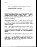 Serf/on 403 Procedural and Monitoring Guidance
4.3.3 Analytical Methods Considerations
Questions to be considered during the choice of an appropriate analytical method include
the parameters of interest, desired detection limits, sample size requirements or restrictions,
methods of preservation, technical and practical holding times, and matrix interferences.
Several USEPA documents (e.g., 1986a and 1986-1991) discuss the common analytical
problems encountered during monitoring analyses of sediment samples. It will frequently be
necessary to use methods other than those currently approved by EPA to achieve a desired
sensitivity in a marine environment. However, alternative methods should be considered
only when they have been demonstrated to provide a level of precision and accuracy
equivalent to or exceeding that of the EPA-approved method. Any proposed changes in
analytical methods should be reviewed by analysts with experience in marine waters.
Chemical Residue Analyses
Several factors determine achievable detection limits for a specific contaminant,
regardless of analytical procedure. These factors include:
• Sample size; 50-100 g (wet weight) with a minimum final dilution volume of
0.5 ml_ is considered adequate (USEPA, 1986-1991).
• Presence of interfering substances.
• Range of pollutants to be analyzed; an optimal method may be developed
without regard to potential effects on other parameters.
• Level of confirmation — qualitative (e.g., presence or absence) or quantitative
(e.g., residue concentrations) analyses.
• Level of pollutant found in the field and in analytical blanks.
A list of analytical procedures and USEPA method numbers is given in Table 4-14.
Selection of appropriate methods should be based on a trade-off between full-scan
analyses, which are economical but cannot provide optimal sensitivity for some
compounds, and alternative methods that are more sensitive for specific compounds but
can result in higher analytical costs. Table 4-15 lists which technique is appropriate for
detecting a specific contaminant.
Metals and Metalloids
Trace element analyses by inductively coupled plasma emission spectrometry (ICP)
allow for several elements to be measured simultaneously. Detection limits of ICP for
most metals are generally comparable to those achieved by graphite furnace atomic
absorption spectrophotometry (GFAA); however, detection limits for several metals (e.g.,
arsenic, selenium, and mercury) are significantly lower using atomic absorption
spectrophotometry (AA).
79
image:
Serf/on 403 Procedural and Monitoring Guidance
4.3.3 Analytical Methods Considerations
Questions to be considered during the choice of an appropriate analytical method include
the parameters of interest, desired detection limits, sample size requirements or restrictions,
methods of preservation, technical and practical holding times, and matrix interferences.
Several USEPA documents (e.g., 1986a and 1986-1991) discuss the common analytical
problems encountered during monitoring analyses of sediment samples. It will frequently be
necessary to use methods other than those currently approved by EPA to achieve a desired
sensitivity in a marine environment. However, alternative methods should be considered
only when they have been demonstrated to provide a level of precision and accuracy
equivalent to or exceeding that of the EPA-approved method. Any proposed changes in
analytical methods should be reviewed by analysts with experience in marine waters.
Chemical Residue Analyses
Several factors determine achievable detection limits for a specific contaminant,
regardless of analytical procedure. These factors include:
• Sample size; 50-100 g (wet weight) with a minimum final dilution volume of
0.5 ml_ is considered adequate (USEPA, 1986-1991).
• Presence of interfering substances.
• Range of pollutants to be analyzed; an optimal method may be developed
without regard to potential effects on other parameters.
• Level of confirmation — qualitative (e.g., presence or absence) or quantitative
(e.g., residue concentrations) analyses.
• Level of pollutant found in the field and in analytical blanks.
A list of analytical procedures and USEPA method numbers is given in Table 4-14.
Selection of appropriate methods should be based on a trade-off between full-scan
analyses, which are economical but cannot provide optimal sensitivity for some
compounds, and alternative methods that are more sensitive for specific compounds but
can result in higher analytical costs. Table 4-15 lists which technique is appropriate for
detecting a specific contaminant.
Metals and Metalloids
Trace element analyses by inductively coupled plasma emission spectrometry (ICP)
allow for several elements to be measured simultaneously. Detection limits of ICP for
most metals are generally comparable to those achieved by graphite furnace atomic
absorption spectrophotometry (GFAA); however, detection limits for several metals (e.g.,
arsenic, selenium, and mercury) are significantly lower using atomic absorption
spectrophotometry (AA).
79
image:
 Methods
Table 4-14. List of Analytical Techniques
(USEPA, 1986a)
METALS/METALLOIDS
• Atomic Absorption Spectrophotometry (AA)
- flame
graphite furnace (GFAA)
cold vapor
gaseous hydride (HYDAA)
• Inductively Coupled Plasma Emission
Spectrometry (ICP)
ORGANICS
• Gas Chromatography (GC)
- with electron capture detection (GC/ECD)
- with mass spectrometry (GC/MS)
USEPA method 7000 series
USEPA method 7470
USEPA methods 7060 and 7740
USEPA method 6010
USEPA method 8080
USEPA methods 8240 and 8270
Pollutants Tested for by Following Techniques:
ICP
Al, Sb, As, Ba, Be, B, Cd, Ca, Cr, Co, Cu, Fe,
Pb, Mg, Mn, Mo, Ni, K, Se, Si, Ag, Na, Tl, V, and
Zn
Al, Sb, As, Ba, Be, Cd, Cr, Co, Cu, Fe, Pb, Mn,
Hg, Mo, Ni, Se, Ag, Tl, Sn, V, and Zn
SOURCE: USEPA, 1986a.
The combination of AA and ICP is the recommended analytical method for detection of
metals and metalloids since no technique is best for all elements (USEPA, 1986a). Cold
vapor AA analysis is the recommended technique for mercury (USEPA, 1986a).
Digestion methods for sediment samples are reviewed by Plumb (1981). The EPA
Contract Laboratory Program requires the use of nitric acid and hydrogen peroxide
(USEPA, 19901).
GFAA is more sensitive (i.e., lower detection limits) than flame AA or ICP, but it is more
subject to matrix and spectral interferences. GFAA requires particular caution with
regard to laboratory contamination. The concentration of each element is determined by
80
image:
Methods
Table 4-14. List of Analytical Techniques
(USEPA, 1986a)
METALS/METALLOIDS
• Atomic Absorption Spectrophotometry (AA)
- flame
graphite furnace (GFAA)
cold vapor
gaseous hydride (HYDAA)
• Inductively Coupled Plasma Emission
Spectrometry (ICP)
ORGANICS
• Gas Chromatography (GC)
- with electron capture detection (GC/ECD)
- with mass spectrometry (GC/MS)
USEPA method 7000 series
USEPA method 7470
USEPA methods 7060 and 7740
USEPA method 6010
USEPA method 8080
USEPA methods 8240 and 8270
Pollutants Tested for by Following Techniques:
ICP
Al, Sb, As, Ba, Be, B, Cd, Ca, Cr, Co, Cu, Fe,
Pb, Mg, Mn, Mo, Ni, K, Se, Si, Ag, Na, Tl, V, and
Zn
Al, Sb, As, Ba, Be, Cd, Cr, Co, Cu, Fe, Pb, Mn,
Hg, Mo, Ni, Se, Ag, Tl, Sn, V, and Zn
SOURCE: USEPA, 1986a.
The combination of AA and ICP is the recommended analytical method for detection of
metals and metalloids since no technique is best for all elements (USEPA, 1986a). Cold
vapor AA analysis is the recommended technique for mercury (USEPA, 1986a).
Digestion methods for sediment samples are reviewed by Plumb (1981). The EPA
Contract Laboratory Program requires the use of nitric acid and hydrogen peroxide
(USEPA, 19901).
GFAA is more sensitive (i.e., lower detection limits) than flame AA or ICP, but it is more
subject to matrix and spectral interferences. GFAA requires particular caution with
regard to laboratory contamination. The concentration of each element is determined by
80
image:
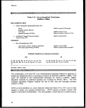 Section 405 Procedural and Monitoring Guidance
Table 4-15. USEPA Organic Contaminant Detection Techniques
USEPA Method3 Contaminant Type Method
8010
8015
8020
8021
8030
8040
8060
8080
8090
8100
8110
8140
8150
8240
8270
Purgeable Halocarbons
Purgeable Nonhalogenated Volatiles
Purgeable Aromatics
Purgeable Organics
Acrolein/Acrylonitrile
Phenols
Phthalate Esters
PCBs and Organochlorine Pesticides
Nitroaromatics and Cyclic Ketones
Polycyclic Aromatic Hydrocarbons
Haloethers
Organophosphorous Pesticides
Chlorinated Herbicides
Volatile Organics
Semivolatile Organics
GC-ELCD
GC-FID
GC-PID
GC-FID and GC-PID
GC-FID and PID
GC-FID
GC-ECD
GC-ECD
GC-FID-ECD '
HPLC-UV-FL or GC-FID
GC-ECD
GC-FPD or NPD
GC-ECD or ELCD
GC-MS
GC-MS
'USEPA, 1986e.
a separate analysis, making the analysis of a large number of contaminant metals both
labor-intensive and relatively expensive compared to ICP. AA methods may, however,
be cost-effective for the analysis of a few metals over a large number of samples.
Semivolatile Organic Compounds
Analysis of Semivolatile organic compounds involves a solvent extraction of the sample,
cleanup of the characteristically complex extract, and gas chromatographic (GC)
analysis and quantitation. There are two gas ehromatography/mass spectrometry
(GC/MS) options for detecting extractable organic compounds: internal standard and
isotope dilution. The isotope dilution technique, which requires spiking the sample with
a mixture of stable isotope-labeled analogs of the analytes, is recommended because
reliable recovery corrections can be made for each analyte with a labeled analog or a
chemically similar analog. The isotope dilution method is more expensive and less
widely employed than the internal standard method, which is the current method of
choice in the Contract Laboratory Program. Mass spectrometry provides positive
compound identification by comparison of both retention time and spectral patterns with
81
image:
Section 405 Procedural and Monitoring Guidance
Table 4-15. USEPA Organic Contaminant Detection Techniques
USEPA Method3 Contaminant Type Method
8010
8015
8020
8021
8030
8040
8060
8080
8090
8100
8110
8140
8150
8240
8270
Purgeable Halocarbons
Purgeable Nonhalogenated Volatiles
Purgeable Aromatics
Purgeable Organics
Acrolein/Acrylonitrile
Phenols
Phthalate Esters
PCBs and Organochlorine Pesticides
Nitroaromatics and Cyclic Ketones
Polycyclic Aromatic Hydrocarbons
Haloethers
Organophosphorous Pesticides
Chlorinated Herbicides
Volatile Organics
Semivolatile Organics
GC-ELCD
GC-FID
GC-PID
GC-FID and GC-PID
GC-FID and PID
GC-FID
GC-ECD
GC-ECD
GC-FID-ECD '
HPLC-UV-FL or GC-FID
GC-ECD
GC-FPD or NPD
GC-ECD or ELCD
GC-MS
GC-MS
'USEPA, 1986e.
a separate analysis, making the analysis of a large number of contaminant metals both
labor-intensive and relatively expensive compared to ICP. AA methods may, however,
be cost-effective for the analysis of a few metals over a large number of samples.
Semivolatile Organic Compounds
Analysis of Semivolatile organic compounds involves a solvent extraction of the sample,
cleanup of the characteristically complex extract, and gas chromatographic (GC)
analysis and quantitation. There are two gas ehromatography/mass spectrometry
(GC/MS) options for detecting extractable organic compounds: internal standard and
isotope dilution. The isotope dilution technique, which requires spiking the sample with
a mixture of stable isotope-labeled analogs of the analytes, is recommended because
reliable recovery corrections can be made for each analyte with a labeled analog or a
chemically similar analog. The isotope dilution method is more expensive and less
widely employed than the internal standard method, which is the current method of
choice in the Contract Laboratory Program. Mass spectrometry provides positive
compound identification by comparison of both retention time and spectral patterns with
81
image:
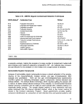 Methods
standard compounds. This technique, however, lacks the sensitivity to detect levels of
most trace contaminants in marine systems. Alternative methods providing greater
sensitivity are available but are compound-specific and, therefore, more expensive.
The identification of many organic compounds can be made by gas chromatography/
electron capture detection (GC/ECD) analysis. GC/ECD provides greater sensitivity
(lower detection limits) relative to GC/MS; however, GC/ECD does not provide positive
compound identification. Since the identity of a compound is determined solely by
matching retention time with that of a standard, confirmation of the initial identity of the
compound on a second GC column is required for confidence in the reliability of the
qualitative identification of the compound. When a compound is present at a high
enough concentration, its identity should be confirmed by the use of GC/MS. GC/ECD
is the method of choice for pesticides and RGBs. Glass capillary GC achieves a much
higher degree of resolution in the analysis of PCB congeners than the standard packed
column methods; however, few laboratories regularly employ this specialized technique.
The detection and concentration of PCBs can be more accurately determined using
comparison mixtures other than the standard industrial Aroclor mixtures. Evaluations of
PCB assemblages in environmental samples by quantification as Aroclors or total PCBs
are of limited accuracy due to environmental degradation and differential affinities of
PCB congeners for different environmental compartments. A more meaningful
evaluation can be accomplished by quantification by PCB isomer groupings (dependent
on the number of chlorine atoms per molecules). This has the advantage of indicating
the relative concentrations of the groups containing the most toxic and bioaccumulating
congeners (McFarland et al., 1986). An alternative method of analysis is to test for the
individual PCB congeners. Using congener-specific methods instead of Aroclor
standard mixtures provides more accurate identification and quantification and
eliminates the necessity of subjective decisions on the part of the analyst (Eganhouse,
1990). However, beside being more expensive and time-consuming, the compatibility of
these enhanced detection methods with the standard Aroclor method is an important
consideration for monitoring programs with existing historical data. All other organic
compound groups are recommended for analysis by GC/MS (USEPA, 1986a).
Volatile Organic Compounds
The purge-and-trap GC/MS technique is employed for detecting volatile organic
compounds in water. A successful variation for detection of volatile organic residues in
sediments involves a device that vaporizes volatile organic compounds from the
sediment sample under vacuum and then condenses the volatiles in a super-cooled trap
(Hiatt, 1981). The trap is then transferred to a purge-and-trap device, where it is treated
as a water sample. The heated purge-and-trap technique, employed in the Contract
Laboratory Program, involves the addition of a weighed amount of sediment to a known
volume of water. As the chamber is heated, inert gas is bubbled through the suspension
to sweep volatile organics out of the sediment. The isotope dilution option is
82
image:
Methods
standard compounds. This technique, however, lacks the sensitivity to detect levels of
most trace contaminants in marine systems. Alternative methods providing greater
sensitivity are available but are compound-specific and, therefore, more expensive.
The identification of many organic compounds can be made by gas chromatography/
electron capture detection (GC/ECD) analysis. GC/ECD provides greater sensitivity
(lower detection limits) relative to GC/MS; however, GC/ECD does not provide positive
compound identification. Since the identity of a compound is determined solely by
matching retention time with that of a standard, confirmation of the initial identity of the
compound on a second GC column is required for confidence in the reliability of the
qualitative identification of the compound. When a compound is present at a high
enough concentration, its identity should be confirmed by the use of GC/MS. GC/ECD
is the method of choice for pesticides and RGBs. Glass capillary GC achieves a much
higher degree of resolution in the analysis of PCB congeners than the standard packed
column methods; however, few laboratories regularly employ this specialized technique.
The detection and concentration of PCBs can be more accurately determined using
comparison mixtures other than the standard industrial Aroclor mixtures. Evaluations of
PCB assemblages in environmental samples by quantification as Aroclors or total PCBs
are of limited accuracy due to environmental degradation and differential affinities of
PCB congeners for different environmental compartments. A more meaningful
evaluation can be accomplished by quantification by PCB isomer groupings (dependent
on the number of chlorine atoms per molecules). This has the advantage of indicating
the relative concentrations of the groups containing the most toxic and bioaccumulating
congeners (McFarland et al., 1986). An alternative method of analysis is to test for the
individual PCB congeners. Using congener-specific methods instead of Aroclor
standard mixtures provides more accurate identification and quantification and
eliminates the necessity of subjective decisions on the part of the analyst (Eganhouse,
1990). However, beside being more expensive and time-consuming, the compatibility of
these enhanced detection methods with the standard Aroclor method is an important
consideration for monitoring programs with existing historical data. All other organic
compound groups are recommended for analysis by GC/MS (USEPA, 1986a).
Volatile Organic Compounds
The purge-and-trap GC/MS technique is employed for detecting volatile organic
compounds in water. A successful variation for detection of volatile organic residues in
sediments involves a device that vaporizes volatile organic compounds from the
sediment sample under vacuum and then condenses the volatiles in a super-cooled trap
(Hiatt, 1981). The trap is then transferred to a purge-and-trap device, where it is treated
as a water sample. The heated purge-and-trap technique, employed in the Contract
Laboratory Program, involves the addition of a weighed amount of sediment to a known
volume of water. As the chamber is heated, inert gas is bubbled through the suspension
to sweep volatile organics out of the sediment. The isotope dilution option is
82
image:
 Section 403 Procedural and Monitoring Guidance
recommended if the data quality objectives (DQOs) of the monitoring program require
accurate quantitation of each compound. This option involves additional analysis time
and expense.
Sediment Toxicity Tests
Toxicity tests may be necessary if the sediment contains contaminants that could result
in an adverse impact on the benthic environment and/or the water column. Tests with
whole sediment are used to determine effects on benthic organisms. Tests with
suspensions of the sediment are used to determine effects on water-column organisms.
Test organisms should be representative of sensitive organisms existing in the vicinity of
the actual site. Mortality of a certain percent of the organisms in the laboratory test does
not imply that the population of the species around the site would decline by the same
percent; however, results can be compared with reference-sediment results to
determine whether the site sediment has higher toxicity (EA and Battelle, 1990).
An introductory guide to toxicity testing is presented in Part 8000 of APHA (1989). Most
of the procedures currently used for sediment toxicity testing are based on USEPA/COE
(1977). Additional discussion and procedures can be found in the draft testing manual
for dredged material (EA and Battelle, 1990) and in USEPA (1986-1991) and Swartz et
al. (1982, 1985).
Acute toxicity tests are conducted to determine the immediate effects of short-term
exposures under specific conditions, providing little information about possible delayed
effects. It can be difficult to apply laboratory results to field situations because of the
fact that motile organisms might avoid exposure when possible and toxicity to benthic
organisms is dependent on field-specific sediment characteristics, the dynamics of
equilibrium partitioning, and routes of exposure. ASTM (1990) proposes standard
guidelines for conducting 10-day static toxicity tests.
4.3.4
QA/QC Considerations
Measurement data are no better than the planning that goes into setting data quality
objectives, choosing appropriate sampling and analysis methodologies, and setting
quality control criteria. An expert chemist and the references cited in this document
should be used to develop a comprehensive QA plan.
Sample Collection
The primary criterion for an adequate sampler is that it consistently collect undisturbed
and uncontaminated samples. The sampling device should be inspected for wear and
tear leading to sample leakage during ascent. It is recommended that a backup sampler
be available on board the survey vessel in case the primary sampler is lost or becomes
inoperable during the cruise.
83
image:
Section 403 Procedural and Monitoring Guidance
recommended if the data quality objectives (DQOs) of the monitoring program require
accurate quantitation of each compound. This option involves additional analysis time
and expense.
Sediment Toxicity Tests
Toxicity tests may be necessary if the sediment contains contaminants that could result
in an adverse impact on the benthic environment and/or the water column. Tests with
whole sediment are used to determine effects on benthic organisms. Tests with
suspensions of the sediment are used to determine effects on water-column organisms.
Test organisms should be representative of sensitive organisms existing in the vicinity of
the actual site. Mortality of a certain percent of the organisms in the laboratory test does
not imply that the population of the species around the site would decline by the same
percent; however, results can be compared with reference-sediment results to
determine whether the site sediment has higher toxicity (EA and Battelle, 1990).
An introductory guide to toxicity testing is presented in Part 8000 of APHA (1989). Most
of the procedures currently used for sediment toxicity testing are based on USEPA/COE
(1977). Additional discussion and procedures can be found in the draft testing manual
for dredged material (EA and Battelle, 1990) and in USEPA (1986-1991) and Swartz et
al. (1982, 1985).
Acute toxicity tests are conducted to determine the immediate effects of short-term
exposures under specific conditions, providing little information about possible delayed
effects. It can be difficult to apply laboratory results to field situations because of the
fact that motile organisms might avoid exposure when possible and toxicity to benthic
organisms is dependent on field-specific sediment characteristics, the dynamics of
equilibrium partitioning, and routes of exposure. ASTM (1990) proposes standard
guidelines for conducting 10-day static toxicity tests.
4.3.4
QA/QC Considerations
Measurement data are no better than the planning that goes into setting data quality
objectives, choosing appropriate sampling and analysis methodologies, and setting
quality control criteria. An expert chemist and the references cited in this document
should be used to develop a comprehensive QA plan.
Sample Collection
The primary criterion for an adequate sampler is that it consistently collect undisturbed
and uncontaminated samples. The sampling device should be inspected for wear and
tear leading to sample leakage during ascent. It is recommended that a backup sampler
be available on board the survey vessel in case the primary sampler is lost or becomes
inoperable during the cruise.
83
image:
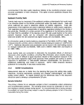 Methods
In the field, sources of contamination include sampling gear, lubricants and oils, engine
exhaust, airborne dust, and ice used for cooling samples. If samples are designated for
chemical analysis, all sampling equipment (e.g., siphon hoses, scoops, containers) must
be made of noncontaminating material and must be cleaned appropriately prior to use.
Potential airborne contamination such as stack gases and cigarette smoke should be
avoided. Furthermore, samples and sampling containers should not be touched with
ungloved fingers.
The following sample acceptability criteria should be satisfied (USEF3A, 1986-1991):
• The sampler is not overfilled with sample so that the sediment surface is
pressed against the top of the sampler.
• Overlying water is present, indicating minimal leakage.
• The overlying water is not excessively turbid, indicating minimal sample
disturbance.
• The sediment surface is relatively flat, indicating minimal disturbance or
winnowing (Figure 4-1).
Acceptable if Minimum
Penetration Requirement Met
and Overlying Water is Present
Unacceptable
(Washed, Rock Caught in Jaws)
Unacceptable
(Canted with Partial Sample)
Unacceptable
(Washed)
Figure 4-1. Examples of Acceptable and Unacceptable Samples
84
image:
Methods
In the field, sources of contamination include sampling gear, lubricants and oils, engine
exhaust, airborne dust, and ice used for cooling samples. If samples are designated for
chemical analysis, all sampling equipment (e.g., siphon hoses, scoops, containers) must
be made of noncontaminating material and must be cleaned appropriately prior to use.
Potential airborne contamination such as stack gases and cigarette smoke should be
avoided. Furthermore, samples and sampling containers should not be touched with
ungloved fingers.
The following sample acceptability criteria should be satisfied (USEF3A, 1986-1991):
• The sampler is not overfilled with sample so that the sediment surface is
pressed against the top of the sampler.
• Overlying water is present, indicating minimal leakage.
• The overlying water is not excessively turbid, indicating minimal sample
disturbance.
• The sediment surface is relatively flat, indicating minimal disturbance or
winnowing (Figure 4-1).
Acceptable if Minimum
Penetration Requirement Met
and Overlying Water is Present
Unacceptable
(Washed, Rock Caught in Jaws)
Unacceptable
(Canted with Partial Sample)
Unacceptable
(Washed)
Figure 4-1. Examples of Acceptable and Unacceptable Samples
84
image:
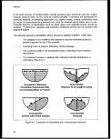 Section 403 Procedural and Monitoring Guidance
• The desired penetration depth is achieved.
If the sample does not meet ail the criteria, it should be rejected.
Splitting of sediment samples for chemical analyses should only be conducted with
noncontaminating tools under "clean room" conditions. Recommended container
materials, sample sizes, preservation techniques, and analytical holding times should be
determined before the sampling effort is undertaken.
For analyses of metals, samples should be frozen and kept at -20°C. Although specific
holding times have not been recommended by EPA, a maximum of 6 months (28 days
for mercury) would be consistent with those for aqueous samples (Table 4-12).
For analyses of volatile compounds, samples should be stored in the dark at 4°C
(USEPA, 1986-1991; USEPA, 1987c). Analyses of volatile compounds should be
performed within 7 days of collection as recommended by EPA. If extractions of
semivolatile compounds will not be performed within 7 days, freezing of the samples at
-20°C is advised. EPA has not established holding times for frozen samples. A general
guideline of a maximum of 6 months would be consistent with that for water samples
(USEPA, 1986-1991).
Samples for determination of TOC or AVS should be analyzed as soon as possible. If
not analyzed immediately, TOC samples should be refrigerated and their pH brought
below 2 by addition of H?_SO4. Acid volatile sulfides should be stored in airtight
containers under an inert atmosphere and analyzed as soon as possible.
Various types of blanks can be prepared and analyzed to identify possible sources of
sample contamination. Field blanks are aqueous samples manipulated in the field.
Rinsate blanks are aqueous samples that are poured over the sampling equipment and
collected. Trip blanks are packed in the sample coolers to detect cross-contamination of
volatile organic compounds.
Blind duplicates, treated and identified as separate samples, may be sent to the same
laboratory for analysis, or one of the pair may be sent to a "reference" laboratory for
comparison. Standard reference material may be prepared and sent as a performance
check to the laboratory. Depending on how these types of samples are handled, they
may be used as a check for accuracy and/or precision.
85
image:
Section 403 Procedural and Monitoring Guidance
• The desired penetration depth is achieved.
If the sample does not meet ail the criteria, it should be rejected.
Splitting of sediment samples for chemical analyses should only be conducted with
noncontaminating tools under "clean room" conditions. Recommended container
materials, sample sizes, preservation techniques, and analytical holding times should be
determined before the sampling effort is undertaken.
For analyses of metals, samples should be frozen and kept at -20°C. Although specific
holding times have not been recommended by EPA, a maximum of 6 months (28 days
for mercury) would be consistent with those for aqueous samples (Table 4-12).
For analyses of volatile compounds, samples should be stored in the dark at 4°C
(USEPA, 1986-1991; USEPA, 1987c). Analyses of volatile compounds should be
performed within 7 days of collection as recommended by EPA. If extractions of
semivolatile compounds will not be performed within 7 days, freezing of the samples at
-20°C is advised. EPA has not established holding times for frozen samples. A general
guideline of a maximum of 6 months would be consistent with that for water samples
(USEPA, 1986-1991).
Samples for determination of TOC or AVS should be analyzed as soon as possible. If
not analyzed immediately, TOC samples should be refrigerated and their pH brought
below 2 by addition of H?_SO4. Acid volatile sulfides should be stored in airtight
containers under an inert atmosphere and analyzed as soon as possible.
Various types of blanks can be prepared and analyzed to identify possible sources of
sample contamination. Field blanks are aqueous samples manipulated in the field.
Rinsate blanks are aqueous samples that are poured over the sampling equipment and
collected. Trip blanks are packed in the sample coolers to detect cross-contamination of
volatile organic compounds.
Blind duplicates, treated and identified as separate samples, may be sent to the same
laboratory for analysis, or one of the pair may be sent to a "reference" laboratory for
comparison. Standard reference material may be prepared and sent as a performance
check to the laboratory. Depending on how these types of samples are handled, they
may be used as a check for accuracy and/or precision.
85
image:
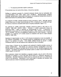 Methods
Laboratory Analyses
Laboratory performance standards as measured by method QC protocols should be
used to evaluate and select appropriate analytical methods. Changes in selected
laboratory protocols should be considered and/or approved only if proposed procedures
meet or exceed established performance criteria. Tables 4-16 and 4-17 provide brief
summaries of QC analyses for laboratory work.
QA reports should describe the results of quantitative QC analyses, as well as other
elements critical to accurate interpretation of analytical results. It is recommended that
these reports be recorded and stored in a database for future reference.
Table 4-16. Summary of Quality Control Analyses
Analysis Type
Recommended Frequency of Analysis
Surrogate Spikes
Method Blank
Standard Reference
Materials
Matrix Spikes
Spiked Method Blanks
Analytical Replicates
Field Replicates
Required in every organic sample - minimum 3
neutral, 2 acid spikes, plus 1 spike for pesticide/PCB
analyses, and 3 spikes for volatiles. Isotope dilution
technique (i.e., with all available labeled surrogates) is
recommended for full-scan analyses and to enable
recovery corrections to be applied to data.
One per extraction batch (semivolatile organics). One
per extraction batch or one per 12-hour shift,
whichever is more frequent (volatile organics).
<50 samples: one per set of samples submitted to lab.
>50 samples: one per 50 samples analyzed.
Not required if complete isotope dilution technique is
used.
<20 samples: one per set of samples submitted to lab.
>20 samples: 5 percent of total number of samples.
As many as required to establish confidence in
method before analysis of samples (i.e., when using a
method for the first time or after any method
modification).
<20 samples: one per set of samples submitted to lab.
>20 samples: 5 percent of total number of samples.
At the discretion of the project coordinator.
toi
.«. fa.
86
image:
Methods
Laboratory Analyses
Laboratory performance standards as measured by method QC protocols should be
used to evaluate and select appropriate analytical methods. Changes in selected
laboratory protocols should be considered and/or approved only if proposed procedures
meet or exceed established performance criteria. Tables 4-16 and 4-17 provide brief
summaries of QC analyses for laboratory work.
QA reports should describe the results of quantitative QC analyses, as well as other
elements critical to accurate interpretation of analytical results. It is recommended that
these reports be recorded and stored in a database for future reference.
Table 4-16. Summary of Quality Control Analyses
Analysis Type
Recommended Frequency of Analysis
Surrogate Spikes
Method Blank
Standard Reference
Materials
Matrix Spikes
Spiked Method Blanks
Analytical Replicates
Field Replicates
Required in every organic sample - minimum 3
neutral, 2 acid spikes, plus 1 spike for pesticide/PCB
analyses, and 3 spikes for volatiles. Isotope dilution
technique (i.e., with all available labeled surrogates) is
recommended for full-scan analyses and to enable
recovery corrections to be applied to data.
One per extraction batch (semivolatile organics). One
per extraction batch or one per 12-hour shift,
whichever is more frequent (volatile organics).
<50 samples: one per set of samples submitted to lab.
>50 samples: one per 50 samples analyzed.
Not required if complete isotope dilution technique is
used.
<20 samples: one per set of samples submitted to lab.
>20 samples: 5 percent of total number of samples.
As many as required to establish confidence in
method before analysis of samples (i.e., when using a
method for the first time or after any method
modification).
<20 samples: one per set of samples submitted to lab.
>20 samples: 5 percent of total number of samples.
At the discretion of the project coordinator.
toi
.«. fa.
86
image:
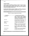 Section 403 Procedural and Monitoring Guidance
Table 4-17. Summary of Warning and Control Limits
for Quality Control Sample
Analysis Type
Recommended
Warning Limit
Recommended
Control Limit
Surrogate Spikes
Method Blank
Phthalate,
Acetone
Other Organic
Compounds
Standard Reference
Materials
Matrix spikes
Spiked Method Blanks
Analytical Replicates
Field Replicates
Ongoing Calibration
10 percent recovery
30 percent of the analyte
1 u.g total or 5 percent
of the analyte
95 percent
confidence interval
50-65 percent recovery
50-65 percent recovery
50 percent recovery
5 u,g total or 5 percent
of the analyte
2.5 (j.g total or 5 percent
of the analyte
95 percent confidence
interval for certified
reference material
50 percent recovery
50 percent recovery
±100 percent
coefficient of variation
25 percent of
initial calibration
Calibration standards should be analyzed at the beginning of sample analysis and
should be verified at the end of each 12-hour shift during which analyses are
performed. The concentrations of calibration standards should bracket the expected
sample concentrations, or sample dilutions or sample handling modifications (i.e.,
reduced sample size) will be required.
Analysis of methods or reagent blanks should be conducted to demonstrate the
absence of contamination from sample handling in the laboratory. At least one
method blank must be included with each batch of samples and should constitute at
87
image:
Section 403 Procedural and Monitoring Guidance
Table 4-17. Summary of Warning and Control Limits
for Quality Control Sample
Analysis Type
Recommended
Warning Limit
Recommended
Control Limit
Surrogate Spikes
Method Blank
Phthalate,
Acetone
Other Organic
Compounds
Standard Reference
Materials
Matrix spikes
Spiked Method Blanks
Analytical Replicates
Field Replicates
Ongoing Calibration
10 percent recovery
30 percent of the analyte
1 u.g total or 5 percent
of the analyte
95 percent
confidence interval
50-65 percent recovery
50-65 percent recovery
50 percent recovery
5 u,g total or 5 percent
of the analyte
2.5 (j.g total or 5 percent
of the analyte
95 percent confidence
interval for certified
reference material
50 percent recovery
50 percent recovery
±100 percent
coefficient of variation
25 percent of
initial calibration
Calibration standards should be analyzed at the beginning of sample analysis and
should be verified at the end of each 12-hour shift during which analyses are
performed. The concentrations of calibration standards should bracket the expected
sample concentrations, or sample dilutions or sample handling modifications (i.e.,
reduced sample size) will be required.
Analysis of methods or reagent blanks should be conducted to demonstrate the
absence of contamination from sample handling in the laboratory. At least one
method blank must be included with each batch of samples and should constitute at
87
image:
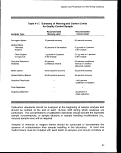 Methods
least 5 percent of all samples analyzed. All blanks should be free of detectable
concentrations of the target compounds, or steps should be taken to remove the source
of contamination before sample analysis proceeds.
Spike recovery analyses are required to assess method performance for the particular
sample matrix. Spike recoveries serve as an indication of analytical accuracy, whereas
analysis of standard reference materials (SRMs) can measure extraction efficiency.
Commonly recommended control limits include 75-125 percent recovery for spikes and
80-120 percent recovery for the analysis of SRMs.
Replicates must be analyzed to monitor the precision of laboratory analyses. A
minimum of 5 percent of the analyses should be laboratory replicates. Field duplicates
should also be collected where practical. Common control limits are ±20 relative
percent difference between duplicates.
Currently, no universally accepted convention for reporting detection limits of analytical
procedures exists. Table 4-11 in the preceding section lists definitions of various
detection limits used by the American Chemical Society's Committee on Environmental
Improvement (CEI). The IDL does not address possible blank contaminants or matrix
interferences and is not a good standard for complex environmental matrices. The LOD
and LOQ account for blanks, but not matrix interferences. The MDL provides high
statistical confidence but, like the LOQ, may be too stringent. Detection limits must be
specified and reported to ensure adequate data quality and comparability between
protocols.
4.3.5 Statistical Design Considerations
Statistical strategies may mitigate the high costs of collecting sufficient samples of
sediment. Power analyses can affect the strategy of compositing samples and can often
lead to a cost-effective monitoring design strategy.
Composite Sampling
Composite sediment sampling consists of mixing samples from two or more replications
collected at a particular location over time or collected at several locations at the same
time. The analysis of a composite sample provides an estimate of an average
contaminant concentration for the locations composing the composite sample.
Advantages of the composite sampling strategy are:
• It provides a cost-effective strategy when individual chemical analyses are
expensive.
• It results in a more efficient estimate of the mean at specified sampling
locations.
88
image:
Methods
least 5 percent of all samples analyzed. All blanks should be free of detectable
concentrations of the target compounds, or steps should be taken to remove the source
of contamination before sample analysis proceeds.
Spike recovery analyses are required to assess method performance for the particular
sample matrix. Spike recoveries serve as an indication of analytical accuracy, whereas
analysis of standard reference materials (SRMs) can measure extraction efficiency.
Commonly recommended control limits include 75-125 percent recovery for spikes and
80-120 percent recovery for the analysis of SRMs.
Replicates must be analyzed to monitor the precision of laboratory analyses. A
minimum of 5 percent of the analyses should be laboratory replicates. Field duplicates
should also be collected where practical. Common control limits are ±20 relative
percent difference between duplicates.
Currently, no universally accepted convention for reporting detection limits of analytical
procedures exists. Table 4-11 in the preceding section lists definitions of various
detection limits used by the American Chemical Society's Committee on Environmental
Improvement (CEI). The IDL does not address possible blank contaminants or matrix
interferences and is not a good standard for complex environmental matrices. The LOD
and LOQ account for blanks, but not matrix interferences. The MDL provides high
statistical confidence but, like the LOQ, may be too stringent. Detection limits must be
specified and reported to ensure adequate data quality and comparability between
protocols.
4.3.5 Statistical Design Considerations
Statistical strategies may mitigate the high costs of collecting sufficient samples of
sediment. Power analyses can affect the strategy of compositing samples and can often
lead to a cost-effective monitoring design strategy.
Composite Sampling
Composite sediment sampling consists of mixing samples from two or more replications
collected at a particular location over time or collected at several locations at the same
time. The analysis of a composite sample provides an estimate of an average
contaminant concentration for the locations composing the composite sample.
Advantages of the composite sampling strategy are:
• It provides a cost-effective strategy when individual chemical analyses are
expensive.
• It results in a more efficient estimate of the mean at specified sampling
locations.
88
image:
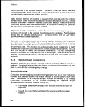 Section 403 Procedural and Monitoring Guidance
Because of the reduced sample variance, composite sampling results in a considerable
increase in statistical power. If the primary objective of a monitoring program is to
determine differences in sediment contaminant concentrations among sampling
locations, composite sampling is an applicable strategy.
Space-bulking consists of sampling from several locations and combining sediment
samples into one or more composite samples. Time-bulking involves taking multiple
samples over time from a single location and compositing these samples. Space- and
time-bulking strategies should be used judiciously since significant information
concerning spatial and temporal heterogeneity may be lost.
Composite sampling is not recommended if the objective of the monitoring program is
based on water quality-based criteria with specified sediment contaminant concentration
limits since this sampling method does not detect the true range of sediment
contaminant concentrations in the environment. The adoption of composite strategies
will depend on the objectives of individual monitoring programs.
Statistical Power
Statistical power increases with an increase in the number of sediment subsamples in
each replicate composite sample. However, with the addition of successive subsamples
to each composite, a diminished return of statistical power exists. For composites of
greater than 10 replications, the increase of power is negligible given typical levels of
data variability.
To improve the power of a statistical test, while keeping the significance level constant,
the sample size should be increased. Because of constraints in cost and time imposed
by the monitoring program, however, this option may not be available. Power analyses
have shown that for a fixed level of sampling effort, a monitoring program's power is
generally increased by collecting more replicates at fewer locations. The number and
distribution of sampling locations required to evaluate the effectiveness of the monitoring
program will be depend on the size and complexity of the discharge.
4.3.6
Use of Data
The results may be used to monitor and evaluate the condition of benthic habitats and to
provide early warnings of potential impacts to the ecosystem. The data generated from
monitoring of the pollutant levels in estuarine sediments should be used in conjunction
with those collected from other physical and biological monitoring. Subsequent
analyses of health risks to human populations and ecological risks to benthic individuals,
populations, and communities may be performed.
89
image:
Section 403 Procedural and Monitoring Guidance
Because of the reduced sample variance, composite sampling results in a considerable
increase in statistical power. If the primary objective of a monitoring program is to
determine differences in sediment contaminant concentrations among sampling
locations, composite sampling is an applicable strategy.
Space-bulking consists of sampling from several locations and combining sediment
samples into one or more composite samples. Time-bulking involves taking multiple
samples over time from a single location and compositing these samples. Space- and
time-bulking strategies should be used judiciously since significant information
concerning spatial and temporal heterogeneity may be lost.
Composite sampling is not recommended if the objective of the monitoring program is
based on water quality-based criteria with specified sediment contaminant concentration
limits since this sampling method does not detect the true range of sediment
contaminant concentrations in the environment. The adoption of composite strategies
will depend on the objectives of individual monitoring programs.
Statistical Power
Statistical power increases with an increase in the number of sediment subsamples in
each replicate composite sample. However, with the addition of successive subsamples
to each composite, a diminished return of statistical power exists. For composites of
greater than 10 replications, the increase of power is negligible given typical levels of
data variability.
To improve the power of a statistical test, while keeping the significance level constant,
the sample size should be increased. Because of constraints in cost and time imposed
by the monitoring program, however, this option may not be available. Power analyses
have shown that for a fixed level of sampling effort, a monitoring program's power is
generally increased by collecting more replicates at fewer locations. The number and
distribution of sampling locations required to evaluate the effectiveness of the monitoring
program will be depend on the size and complexity of the discharge.
4.3.6
Use of Data
The results may be used to monitor and evaluate the condition of benthic habitats and to
provide early warnings of potential impacts to the ecosystem. The data generated from
monitoring of the pollutant levels in estuarine sediments should be used in conjunction
with those collected from other physical and biological monitoring. Subsequent
analyses of health risks to human populations and ecological risks to benthic individuals,
populations, and communities may be performed.
89
image:
 Methods
Sediment pollutant loading data should be used in combination with other monitoring
methods to assess the condition of the benthic habitat or to guide the decision-making
process. Data acquired from monitoring sediment contaminant levels, in conjunction
with the sediment's physical properties, may be used to assess the bioavailability of
these pollutants. Subsequent analysis of this information along with biological data may
be used to assess the impacts and risks of sediment pollutants to human populations,
benthic populations/communities, and the ecosystem.
Monitoring of pollutant levels in sediments is a widely-accepted means of measuring the
condition of the benthic habitat and is a powerful tool in the evaluation of spatial and
temporal effects of anthropogenic and natural disturbance. However, for sediment
chemistry data to be useful in interpreting toxicological response or in predicting
environmental risks from sediment exposure, sediment criteria are needed. The
Washington State Department of Ecology (1991) has adopted sediment criteria, and
EPA has recently published a sediment compendium (USEPA, 1992). Both of these
documents may provide useful guidance. The ability to extrapolate from sediment
chemistry data to predictions of ecological or human health risks is, however, greatly
limited by a limited understanding of causal relationships between exposure and
response.
4.3.7 Summary and Recommendations
Rationale
• The sediments represent the ultimate sink for many chemical contaminants
from offshore discharges.
• The objective of monitoring bulk sediment chemistry is to detect and describe
spatial and temporal changes of these sediment pollutants.
Monitoring Design Considerations
• It is recommended that types of sampling gear and location and timing of
sample collection be consistent to allow for comparisons among studies.
• Collection of undisturbed sediment requires that the sampler:
- create a minimal bow wake when descending;
- form a leakproof seal when the sediment sample is taken;
- prevent winnowing and excessive sample disturbance when ascending; and
- allow easy access to the sample surface in order that undisturbed
subsamples may be taken.
• In general, analysis of the upper 2 cm is advised to examine recent sediment
contamination events; however, site-specific conditions and program
objectives should be considered when a sampling depth is selected.
90
image:
Methods
Sediment pollutant loading data should be used in combination with other monitoring
methods to assess the condition of the benthic habitat or to guide the decision-making
process. Data acquired from monitoring sediment contaminant levels, in conjunction
with the sediment's physical properties, may be used to assess the bioavailability of
these pollutants. Subsequent analysis of this information along with biological data may
be used to assess the impacts and risks of sediment pollutants to human populations,
benthic populations/communities, and the ecosystem.
Monitoring of pollutant levels in sediments is a widely-accepted means of measuring the
condition of the benthic habitat and is a powerful tool in the evaluation of spatial and
temporal effects of anthropogenic and natural disturbance. However, for sediment
chemistry data to be useful in interpreting toxicological response or in predicting
environmental risks from sediment exposure, sediment criteria are needed. The
Washington State Department of Ecology (1991) has adopted sediment criteria, and
EPA has recently published a sediment compendium (USEPA, 1992). Both of these
documents may provide useful guidance. The ability to extrapolate from sediment
chemistry data to predictions of ecological or human health risks is, however, greatly
limited by a limited understanding of causal relationships between exposure and
response.
4.3.7 Summary and Recommendations
Rationale
• The sediments represent the ultimate sink for many chemical contaminants
from offshore discharges.
• The objective of monitoring bulk sediment chemistry is to detect and describe
spatial and temporal changes of these sediment pollutants.
Monitoring Design Considerations
• It is recommended that types of sampling gear and location and timing of
sample collection be consistent to allow for comparisons among studies.
• Collection of undisturbed sediment requires that the sampler:
- create a minimal bow wake when descending;
- form a leakproof seal when the sediment sample is taken;
- prevent winnowing and excessive sample disturbance when ascending; and
- allow easy access to the sample surface in order that undisturbed
subsamples may be taken.
• In general, analysis of the upper 2 cm is advised to examine recent sediment
contamination events; however, site-specific conditions and program
objectives should be considered when a sampling depth is selected.
90
image:
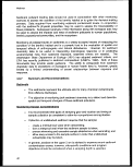 Section 403 Procedural and Monitoring Guidance
• Penetration well below the desired sampling depth is preferred to prevent
sample disturbance as the device closes.
• Total organic carbon and acid volatile sulfide normalizations are
recommended to allow comparisons of chemical residue concentrations
between locations. Normalizing the data will depend on the objectives of the
individual monitoring program.
• It is recommended that sediments be sampled when contamination
concentrations are expected to be at their highest levels.
Analytical Methods Considerations
• It is recommended that consistent analytical protocols be implemented to
allow for comparisons between studies.
• Laboratories should perform acceptably on standard reference materials and
intercalibration exercises before performing routine analyses.
• Periodic full-scan analyses should be undertaken to identify any new
pollutants that should be monitored.
• Metals/Metalloids
- The combination of GFAA and ICP is the recommended method for the
detection of metals and metalloids.
- Cold vapor AA is the recommended protocol for mercury detection.
• Organics
- GC/MS in conjunction with isotope dilution is recommended for the
detection of semivolatile and volatile organic compounds because it
provides reliable recovery data for each analyte.
- A vacuum super-cooled trap in conjunction with a purge-and-trap device
is recommended for the detection of volatile organics.
• Sediment Toxicity Tests
- May be necessary if the sediment contains contaminants that could result
in an adverse impact on the benthic environment and/or the water column.
- Results can be compared with reference-sediment test results to
determine whether the site sediment has higher toxicity.
QA/QC Considerations
• The primary criterion for acceptable field sampling equipment and protocols is
the collection of undisturbed and uncontaminated environmental samples.
91
image:
Section 403 Procedural and Monitoring Guidance
• Penetration well below the desired sampling depth is preferred to prevent
sample disturbance as the device closes.
• Total organic carbon and acid volatile sulfide normalizations are
recommended to allow comparisons of chemical residue concentrations
between locations. Normalizing the data will depend on the objectives of the
individual monitoring program.
• It is recommended that sediments be sampled when contamination
concentrations are expected to be at their highest levels.
Analytical Methods Considerations
• It is recommended that consistent analytical protocols be implemented to
allow for comparisons between studies.
• Laboratories should perform acceptably on standard reference materials and
intercalibration exercises before performing routine analyses.
• Periodic full-scan analyses should be undertaken to identify any new
pollutants that should be monitored.
• Metals/Metalloids
- The combination of GFAA and ICP is the recommended method for the
detection of metals and metalloids.
- Cold vapor AA is the recommended protocol for mercury detection.
• Organics
- GC/MS in conjunction with isotope dilution is recommended for the
detection of semivolatile and volatile organic compounds because it
provides reliable recovery data for each analyte.
- A vacuum super-cooled trap in conjunction with a purge-and-trap device
is recommended for the detection of volatile organics.
• Sediment Toxicity Tests
- May be necessary if the sediment contains contaminants that could result
in an adverse impact on the benthic environment and/or the water column.
- Results can be compared with reference-sediment test results to
determine whether the site sediment has higher toxicity.
QA/QC Considerations
• The primary criterion for acceptable field sampling equipment and protocols is
the collection of undisturbed and uncontaminated environmental samples.
91
image:
 Methods
• Adequate sampling containers and preservation techniques must be used
and appropriate holding times followed to ensure the integrity of samples and
their analyses.
• Blank, spike, and replicate analyses are recommended quality control checks.
• A report describing the objectives of the analytical effort; methods of sample
collection, handling, and preservation; details of the analytical methods;
problems encountered during the analytical process; any necessary
modifications to the written procedures; and results of the QC analyses
should be included with the analytical data.
Statistical Design Considerations
• Compositing of sediments consists of mixing two or more samples collected
at a particular location and/or time period.
• Space-bulking (combining composites from several locations) and
time-bulking (combining several composites over time from one location)
should be used judiciously since information concerning spatial or temporal
heterogeneity may be lost.
• Power analyses have shown that for a fixed level of sampling effort, a
monitoring program's power is generally increased by collecting more
replicates at fewer locations.
Use of Data
• The data gathered from monitoring of the pollutant levels in marine sediments
should be used in conjunction with those collected from other physical and
biological monitoring to monitor rates of recovery following environmental
interventions, to evaluate the condition of benthic habitats, and to provide
early warnings of potential impacts to the estuarine ecosystem.
• Sediment pollutant loading data should be used in combination with other
monitoring methods to assess the condition of the benthic habitat or to guide
the decision-making process.
92
image:
Methods
• Adequate sampling containers and preservation techniques must be used
and appropriate holding times followed to ensure the integrity of samples and
their analyses.
• Blank, spike, and replicate analyses are recommended quality control checks.
• A report describing the objectives of the analytical effort; methods of sample
collection, handling, and preservation; details of the analytical methods;
problems encountered during the analytical process; any necessary
modifications to the written procedures; and results of the QC analyses
should be included with the analytical data.
Statistical Design Considerations
• Compositing of sediments consists of mixing two or more samples collected
at a particular location and/or time period.
• Space-bulking (combining composites from several locations) and
time-bulking (combining several composites over time from one location)
should be used judiciously since information concerning spatial or temporal
heterogeneity may be lost.
• Power analyses have shown that for a fixed level of sampling effort, a
monitoring program's power is generally increased by collecting more
replicates at fewer locations.
Use of Data
• The data gathered from monitoring of the pollutant levels in marine sediments
should be used in conjunction with those collected from other physical and
biological monitoring to monitor rates of recovery following environmental
interventions, to evaluate the condition of benthic habitats, and to provide
early warnings of potential impacts to the estuarine ecosystem.
• Sediment pollutant loading data should be used in combination with other
monitoring methods to assess the condition of the benthic habitat or to guide
the decision-making process.
92
image:
 Section 403 Procedural and Monitoring Guidance
4.4
SEDIMENT GRAIN SIZE
The objective of monitoring sediment grain size composition is to help describe spatial
and temporal changes in the benthic community habitat. Grain size analysis measures
the frequency distribution of particle size ranges composing the sediment. The size
categories (in descending order) are gravel, sand, silt, and clay (Folk, 1980; Plumb,
1981). Sediment contaminants adsorb to small grain surfaces, and the availability of
sediment contaminants may be correlated with the grain size composition of the benthic
sediments.
4.4.1
Rationale
Of the 10 guidelines used to determine unreasonable degradation or irreparable harm,
the following can be assessed by evaluating sediment grain size:
• Quantities, composition, and potential bioaccumulation or persistence of the
pollutants to be discharged and
• Potential transport of the pollutants by biological, physical, or chemical
processes.
Results from sediment chemical monitoring can be normalized according to sediment
characteristics to account for some of the variability found in bioaccumulation rates.
Also, grain size information may be used to aid in the analysis of the temporal and
spatial variability of benthic assemblages since the ability of infaunal organisms to build
tubes, burrow, capture food, and escape predation is affected by grain size. The results
may be used to monitor rates of recovery following an event, to evaluate the condition of
benthic habitats, and to assist in providing early warnings of potential impacts to the
marine environment.
4.4.2 Monitoring Design Considerations
Sediment Sampling Devices
Sampling for sediment grain size is usually undertaken in conjunction with sediment
chemistry and benthic infauna measurements. Thus, the sampling devices and
techniques are similar for all three. In the past, sediment samples have been collected
using a wide range of methods and samplers. Since sample collection protocols
influence all subsequent laboratory and data analysis, it is essential that sediment
samples be collected using acceptable and standardized techniques (USEPA,
1986-1991).
A variety of devices can be used to collect sediment samples, and these fall under two
main categories: grab samplers and core samplers (Mclntyre et al., 1984; ASTM, 1991).
Each device samples the benthic habitat in a different manner (Table 4-18); therefore,
comparisons among dat%collected using different devices is not recommended.
93
image:
Section 403 Procedural and Monitoring Guidance
4.4
SEDIMENT GRAIN SIZE
The objective of monitoring sediment grain size composition is to help describe spatial
and temporal changes in the benthic community habitat. Grain size analysis measures
the frequency distribution of particle size ranges composing the sediment. The size
categories (in descending order) are gravel, sand, silt, and clay (Folk, 1980; Plumb,
1981). Sediment contaminants adsorb to small grain surfaces, and the availability of
sediment contaminants may be correlated with the grain size composition of the benthic
sediments.
4.4.1
Rationale
Of the 10 guidelines used to determine unreasonable degradation or irreparable harm,
the following can be assessed by evaluating sediment grain size:
• Quantities, composition, and potential bioaccumulation or persistence of the
pollutants to be discharged and
• Potential transport of the pollutants by biological, physical, or chemical
processes.
Results from sediment chemical monitoring can be normalized according to sediment
characteristics to account for some of the variability found in bioaccumulation rates.
Also, grain size information may be used to aid in the analysis of the temporal and
spatial variability of benthic assemblages since the ability of infaunal organisms to build
tubes, burrow, capture food, and escape predation is affected by grain size. The results
may be used to monitor rates of recovery following an event, to evaluate the condition of
benthic habitats, and to assist in providing early warnings of potential impacts to the
marine environment.
4.4.2 Monitoring Design Considerations
Sediment Sampling Devices
Sampling for sediment grain size is usually undertaken in conjunction with sediment
chemistry and benthic infauna measurements. Thus, the sampling devices and
techniques are similar for all three. In the past, sediment samples have been collected
using a wide range of methods and samplers. Since sample collection protocols
influence all subsequent laboratory and data analysis, it is essential that sediment
samples be collected using acceptable and standardized techniques (USEPA,
1986-1991).
A variety of devices can be used to collect sediment samples, and these fall under two
main categories: grab samplers and core samplers (Mclntyre et al., 1984; ASTM, 1991).
Each device samples the benthic habitat in a different manner (Table 4-18); therefore,
comparisons among dat%collected using different devices is not recommended.
93
image:
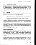 Methods
Table 4-18. Summary of Bottom Sampling Equipment3
Device
Use
Advantages
Disadvantages
Fluorocarbon plastic
or glass
tube
Shallow wadable waters
or deep waters if
SCUBA available. Soft
or semiconsolidated
deposits.
Preserves layering and
permits historical sudy of
sediment deposition.
Rapid-samples immed-
iately ready for laboratory
shipment. Minimal risk of
contamination.
Small sample size requires
repetitive sampling.
Hand corer with
removable
fluorocarbon plastic
or glass liners
Same as above except
more consolidated sedi-
ments can be obtained.
Handles provide for greater
ease of substrate
penetration. Above
advantages.
Careful handling necessary to
prevent spillage, Requires
removal of liners before repetitive
sampling. Slight risk of metal
contamination from barrel and
core cutter.
Box corer
Gravity corers, that
is, Phleger corer
Young grab (fluoro-
carbon plastic- or
Kynar-lined modi-
fied 0.1 m2 Van
Veen)
Ekman or box
dredge
Same as above.
Semiconsolidated
sediments.
Collection of large
undisturbed sample
allowing for subsampling.
Low risk of undisturbed
sample contamination.
Maintains sediment
integrity relatively well.
Lakes and marine areas. Eliminates metal
contamination. Reduces
pressure wave.
Soft to semisoft
sediments. Can be
used from boat, bridge,
or pier in waters of
various depths.
Obtains a larger sample
than coring tubes. Can be
subsampled through box
lid.
Hard to handle.
Careful handling necessary to
avoid sediment spillage. Small
sample, requires repetitive
operation and removal of liners.
Tirne-consuming.
Expensive. Requires winch.
Possible incomplete jaw closure
and sample loss. Possible shock
wave, which may disturb the fine
sediments ("fines"). Metal
construction may introduce
contaminants. Possible loss of
"fines" on retrieval.
Ponar grab
sampler
Useful on sand, silt,
or clay.
Most universal grab
sampler. Adequate on most
substrates. Large sample
obtained intact, permitting
subsampling.
Shock wave from descent may
disturb "fines." Possible
incomplete closure of jaws results
in sample loss. Possible
contamination from metal frame
construction. Sample must be
further prepared for analysis.
94
image:
Methods
Table 4-18. Summary of Bottom Sampling Equipment3
Device
Use
Advantages
Disadvantages
Fluorocarbon plastic
or glass
tube
Shallow wadable waters
or deep waters if
SCUBA available. Soft
or semiconsolidated
deposits.
Preserves layering and
permits historical sudy of
sediment deposition.
Rapid-samples immed-
iately ready for laboratory
shipment. Minimal risk of
contamination.
Small sample size requires
repetitive sampling.
Hand corer with
removable
fluorocarbon plastic
or glass liners
Same as above except
more consolidated sedi-
ments can be obtained.
Handles provide for greater
ease of substrate
penetration. Above
advantages.
Careful handling necessary to
prevent spillage, Requires
removal of liners before repetitive
sampling. Slight risk of metal
contamination from barrel and
core cutter.
Box corer
Gravity corers, that
is, Phleger corer
Young grab (fluoro-
carbon plastic- or
Kynar-lined modi-
fied 0.1 m2 Van
Veen)
Ekman or box
dredge
Same as above.
Semiconsolidated
sediments.
Collection of large
undisturbed sample
allowing for subsampling.
Low risk of undisturbed
sample contamination.
Maintains sediment
integrity relatively well.
Lakes and marine areas. Eliminates metal
contamination. Reduces
pressure wave.
Soft to semisoft
sediments. Can be
used from boat, bridge,
or pier in waters of
various depths.
Obtains a larger sample
than coring tubes. Can be
subsampled through box
lid.
Hard to handle.
Careful handling necessary to
avoid sediment spillage. Small
sample, requires repetitive
operation and removal of liners.
Tirne-consuming.
Expensive. Requires winch.
Possible incomplete jaw closure
and sample loss. Possible shock
wave, which may disturb the fine
sediments ("fines"). Metal
construction may introduce
contaminants. Possible loss of
"fines" on retrieval.
Ponar grab
sampler
Useful on sand, silt,
or clay.
Most universal grab
sampler. Adequate on most
substrates. Large sample
obtained intact, permitting
subsampling.
Shock wave from descent may
disturb "fines." Possible
incomplete closure of jaws results
in sample loss. Possible
contamination from metal frame
construction. Sample must be
further prepared for analysis.
94
image:
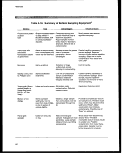 Section 403 Procedural and Monitoring Guidance
Table 4-18. (continued)
Device
Use
Advantages
Disadvantages
BMH-53 piston
corer
Waters of 4-6 ft depth
when used with
extension rod. Soft to
semiconsolidated
deposits.
Piston provides for greater
sample retention.
Cores must be extruded on site to
other containers. Metal barrels
introduce risk of metal
contamination.
Van Veen
BMH-60
Useful on sand, silt, or
clay.
Sampling moving
waters from a fixed
platform.
Adequate on most
substrates. Large sample
obtained intact, permitting
subsampling.
Streamlined configuration
allows sampling where
other devices could not
achieve proper orien-
tiation.
Shock wave from descent may
disturb "fines." Possible
incomplete closure of jaws results
in sample loss. Possible
contamination from metal frame
construction. Sample must be •
further prepared for analysis.
Possible contamination from
metal construction. Subsampling
difficult. Not effective for sampling
fine sediments.
Petersen grab
sampler
Useful on most
substrates.
Large sample; can
penetrate most substrates.
Heavy, may require winch. No
cover lid to permit subsampling.
All other disadvantages of Ekman
and Ponar.
Shipek grab
sampler
Used primarily in
marine waters and large
inland lakes and
reservoirs.
Sample bucket may be
opened to permit
subsampling. Retains
fine-grained sediments
effectively.
Possible contamination from
metal construction. Heavy, may
require winch. Tends to roll over
sample.
Orange-peel grab
Smith-Mclntyre
grab
Useful on most
substrates.
Designed for sampling hard
substrates.
Loss of "fines." Heavy, may
require winch. Possible metal
contamination.
Scoops, drag buckets Various environments
depending on depth
and substrate.
Inexpensive, easy to
handle.
Loss offines" on retrieval
through water column.
Vibratory Corer
Used primarily for
sandy unconsolidated
sediments
Operational at all depths.
Easily transported by truck
and ship. Can penetrate
deeper than conventional
corers.
Has rarely been used for the
study of environmental pollution.
aComments represent subjective evaluations.
SOURCE: ASTM, 1991.
95
image:
Section 403 Procedural and Monitoring Guidance
Table 4-18. (continued)
Device
Use
Advantages
Disadvantages
BMH-53 piston
corer
Waters of 4-6 ft depth
when used with
extension rod. Soft to
semiconsolidated
deposits.
Piston provides for greater
sample retention.
Cores must be extruded on site to
other containers. Metal barrels
introduce risk of metal
contamination.
Van Veen
BMH-60
Useful on sand, silt, or
clay.
Sampling moving
waters from a fixed
platform.
Adequate on most
substrates. Large sample
obtained intact, permitting
subsampling.
Streamlined configuration
allows sampling where
other devices could not
achieve proper orien-
tiation.
Shock wave from descent may
disturb "fines." Possible
incomplete closure of jaws results
in sample loss. Possible
contamination from metal frame
construction. Sample must be •
further prepared for analysis.
Possible contamination from
metal construction. Subsampling
difficult. Not effective for sampling
fine sediments.
Petersen grab
sampler
Useful on most
substrates.
Large sample; can
penetrate most substrates.
Heavy, may require winch. No
cover lid to permit subsampling.
All other disadvantages of Ekman
and Ponar.
Shipek grab
sampler
Used primarily in
marine waters and large
inland lakes and
reservoirs.
Sample bucket may be
opened to permit
subsampling. Retains
fine-grained sediments
effectively.
Possible contamination from
metal construction. Heavy, may
require winch. Tends to roll over
sample.
Orange-peel grab
Smith-Mclntyre
grab
Useful on most
substrates.
Designed for sampling hard
substrates.
Loss of "fines." Heavy, may
require winch. Possible metal
contamination.
Scoops, drag buckets Various environments
depending on depth
and substrate.
Inexpensive, easy to
handle.
Loss offines" on retrieval
through water column.
Vibratory Corer
Used primarily for
sandy unconsolidated
sediments
Operational at all depths.
Easily transported by truck
and ship. Can penetrate
deeper than conventional
corers.
Has rarely been used for the
study of environmental pollution.
aComments represent subjective evaluations.
SOURCE: ASTM, 1991.
95
image:
 Methods
The collection of undisturbed sediment requires that the sampler:
• Create a minimal bow wake when descending;
• Form a leakproof seal when the sediment sample is taken;
• Prevent winnowing and excessive sample disturbance when ascending; and
• Allow easy access to the sample surface so undisturbed samples may be
taken.
Penetration well below the desired sampling depth is preferred to prevent sample
disturbance as the device closes. It is best to use a sampler with a weight adjustment to
enable the modification of penetration depths.
Grab Samplers
Grabs are capable of consistent sampling of bottom habitats. Depending on the size of
the device, areas from 0.02 to 0.5 m2 and depths ranging from 5 to 15 cm may be
sampled. Limitations of grab samplers include :
• Variability in penetration depth among samples depending on sediment
properties;
• Oblique angles of penetration, which result in varying penetration depths
within a sample; and
• Folding of the sample, which results in the inability to section the sample and
the loss of information concerning the vertical structure in the sediments.
The careful use of these devices, however, will provide quantitative data. Grab
samplers are the tools of choice for a number of marine monitoring programs (Fredette
etal., 1989; USEPA, 1986-1991).
Core Samplers
Box corers use a surrounding frame to ensure vertical entry and, therefore, vertical
sectioning of the sample (USEPA, 1986-1991). These devices are capable of maximum
penetration depths of 15 cm and may collect volumes 5 to 10 times those of grab
samplers. Limitations of box corers include :
• Large size and weight, which require the use of cranes or winches and a
large vessel for deployment;
• Higher construction expenses; and
• Lack of calibration studies to permit comparisons to grab samples.
96
image:
Methods
The collection of undisturbed sediment requires that the sampler:
• Create a minimal bow wake when descending;
• Form a leakproof seal when the sediment sample is taken;
• Prevent winnowing and excessive sample disturbance when ascending; and
• Allow easy access to the sample surface so undisturbed samples may be
taken.
Penetration well below the desired sampling depth is preferred to prevent sample
disturbance as the device closes. It is best to use a sampler with a weight adjustment to
enable the modification of penetration depths.
Grab Samplers
Grabs are capable of consistent sampling of bottom habitats. Depending on the size of
the device, areas from 0.02 to 0.5 m2 and depths ranging from 5 to 15 cm may be
sampled. Limitations of grab samplers include :
• Variability in penetration depth among samples depending on sediment
properties;
• Oblique angles of penetration, which result in varying penetration depths
within a sample; and
• Folding of the sample, which results in the inability to section the sample and
the loss of information concerning the vertical structure in the sediments.
The careful use of these devices, however, will provide quantitative data. Grab
samplers are the tools of choice for a number of marine monitoring programs (Fredette
etal., 1989; USEPA, 1986-1991).
Core Samplers
Box corers use a surrounding frame to ensure vertical entry and, therefore, vertical
sectioning of the sample (USEPA, 1986-1991). These devices are capable of maximum
penetration depths of 15 cm and may collect volumes 5 to 10 times those of grab
samplers. Limitations of box corers include :
• Large size and weight, which require the use of cranes or winches and a
large vessel for deployment;
• Higher construction expenses; and
• Lack of calibration studies to permit comparisons to grab samples.
96
image:
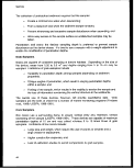 Section 403 Procedural and Monitoring Guidance
The Hessler-Sandia box corer uses dividers to section the core into subsections,
facilitating subsampling of the core. Box corers are recognized as the tools of choice for
maximum accuracy and precision when sampling soft-bottom habitats.
Sediment Profiling Camera
The sediment profiling camera allows vertical in situ imaging of the water-sediment
interface, from which grain size determinations may be conducted. Sediment grain size
determinations may be made at a maximum depth of 18 cm; however, penetration depth
of the viewing prism may be limited because of the physical characteristics of the
sediment (i.e., penetration depths are greater in silt than in sand).
Distinctions between finer silts and clays are not possible. Furthermore, it is
recommended that quantitative calculations of sediment grain size from the image be
ground-truthed (verified) by the results of laboratory analysis of collected sediment
samples.
Although the singular use of the sediment profiling camera is not recommended, the
camera may be effective as a reconnaissance tool. Delineation of habitats with similar
physical characteristics may aid in the selection of appropriate sampling stations.
Recommendations
Collection of sediments and collection of benthic organisms should be done concurrently
to mitigate the costs of field sampling and to permit sound correlation, regression, and
multivariate analyses (see Section 4.5, Benthic Community Structure). Therefore, it is
recommended that the sampling device also be suitable for benthic sampling. Grab and
core sampling devices permit adequate sampling of both sediment and benthic infaunal
communities with one sampling device.
Sample Depth
For characterizing surficial sediments, it is recommended that the upper 2 cm of the
sediment column be evaluated; however, a minimum penetration depth of 4-5 cm should
be achieved. Although the 2 cm specification is arbitrary, it does ensure that relatively
recent sediments are sampled, that adequate volumes of sediment can be obtained
using readily available samplers, and that data from different studies can be compared.
Penetration depth is a function of sediment type and is greatest in fine sediments and
least in coarse sediments. Sampling devices generally rely on either gravity or a piston
mechanism to penetrate sediments. Ideally, the penetration depth can be varied by
adding or subtracting weight from the sampler, but if the sampler cannot be made to
consistently achieve the desired depth, an alternative device should be used (USEPA,
1986-1991).
97
image:
Section 403 Procedural and Monitoring Guidance
The Hessler-Sandia box corer uses dividers to section the core into subsections,
facilitating subsampling of the core. Box corers are recognized as the tools of choice for
maximum accuracy and precision when sampling soft-bottom habitats.
Sediment Profiling Camera
The sediment profiling camera allows vertical in situ imaging of the water-sediment
interface, from which grain size determinations may be conducted. Sediment grain size
determinations may be made at a maximum depth of 18 cm; however, penetration depth
of the viewing prism may be limited because of the physical characteristics of the
sediment (i.e., penetration depths are greater in silt than in sand).
Distinctions between finer silts and clays are not possible. Furthermore, it is
recommended that quantitative calculations of sediment grain size from the image be
ground-truthed (verified) by the results of laboratory analysis of collected sediment
samples.
Although the singular use of the sediment profiling camera is not recommended, the
camera may be effective as a reconnaissance tool. Delineation of habitats with similar
physical characteristics may aid in the selection of appropriate sampling stations.
Recommendations
Collection of sediments and collection of benthic organisms should be done concurrently
to mitigate the costs of field sampling and to permit sound correlation, regression, and
multivariate analyses (see Section 4.5, Benthic Community Structure). Therefore, it is
recommended that the sampling device also be suitable for benthic sampling. Grab and
core sampling devices permit adequate sampling of both sediment and benthic infaunal
communities with one sampling device.
Sample Depth
For characterizing surficial sediments, it is recommended that the upper 2 cm of the
sediment column be evaluated; however, a minimum penetration depth of 4-5 cm should
be achieved. Although the 2 cm specification is arbitrary, it does ensure that relatively
recent sediments are sampled, that adequate volumes of sediment can be obtained
using readily available samplers, and that data from different studies can be compared.
Penetration depth is a function of sediment type and is greatest in fine sediments and
least in coarse sediments. Sampling devices generally rely on either gravity or a piston
mechanism to penetrate sediments. Ideally, the penetration depth can be varied by
adding or subtracting weight from the sampler, but if the sampler cannot be made to
consistently achieve the desired depth, an alternative device should be used (USEPA,
1986-1991).
97
image:
 Methods
Sampling of depths other than 2 cm or vertical stratification of deeper sediment cores
may be appropriate, depending on the objectives of the monitoring program and the rate
of sediment accumulation. For example, if information concerning only the most recent
sedimentation events is required, examination of the upper 1 cm may be appropriate.
Stratification of deeper cores will provide historical data of sediment grain size and
depositional events. If the potential for bioaccumulation of contaminants in infaunal
organisms is a concern, sampling to the depth of the anoxic layer is desirable.
Comparison of data from studies analyzing different sediment depths is not advised.
Sampler penetration well below the desired sampling depth is preferred to prevent
sample disturbance as the device closes.
Selection of Time of Sampling
Sediment grain size compositions are often temporally stable, although some slight
seasonal variability may be present. Changes are usually associated with seasonal
patterns of benthic turbulent mixing and sediment transport phenomena. The frequency
of sampling should be related to the expected rate of change in grain size compositions.
A consistent sampling period is recommended in order that spatial and temporal
comparisons may be made.
If seasonal variations are exhibited, it is recommended that direct comparisons between
samples collected during different seasons be avoided. Studies investigating
interannual variation in the percent composition of grain sizes should be conducted
during the same season (preferably the same month) each year. Furthermore, it is
recommended that grain size be sampled under all discharge conditions so that
changes in the sediment composition due to discharge loading can be tracked.
4.4.3 Analytical Methods Considerations
Sediment grain size may be expressed in either millimeters (mm) or phi (<&) units.
These scales are related according to the equation: <I> = -Iog2 (mm). Data should be
converted to phi units before calculation of grain size parameters. Sediments are
broadly classified into three size classes: silts and clays are less than 0.064 mm (4 <&)
in diameter, sands range from 0.064 mm (4 O) to 1 mm (0 <&) in diameter, and gravels
are larger than 1 mm (Shepard, 1954; Folk, 1974). Grain size is normally reported as
the mean (Mz), although the median grain size (Md-) is sometimes used. Sorting is a
measure of the spread of the grain size distribution. Buller and McManus (1979) provide
a good review of the methodological and statistical analysis of sediment samples.
Particle size determination can either include or exclude organic material. If organic
material is removed prior to analysis, the "true" particle size distribution is determined. If
organic material is included in the analysis, the "apparent1 particle size distribution is
ascertained. Most organic material is in the silt/clay size range and can be removed
from the sediment either by acid washing or ashing. If organic material is left in the
98
image:
Methods
Sampling of depths other than 2 cm or vertical stratification of deeper sediment cores
may be appropriate, depending on the objectives of the monitoring program and the rate
of sediment accumulation. For example, if information concerning only the most recent
sedimentation events is required, examination of the upper 1 cm may be appropriate.
Stratification of deeper cores will provide historical data of sediment grain size and
depositional events. If the potential for bioaccumulation of contaminants in infaunal
organisms is a concern, sampling to the depth of the anoxic layer is desirable.
Comparison of data from studies analyzing different sediment depths is not advised.
Sampler penetration well below the desired sampling depth is preferred to prevent
sample disturbance as the device closes.
Selection of Time of Sampling
Sediment grain size compositions are often temporally stable, although some slight
seasonal variability may be present. Changes are usually associated with seasonal
patterns of benthic turbulent mixing and sediment transport phenomena. The frequency
of sampling should be related to the expected rate of change in grain size compositions.
A consistent sampling period is recommended in order that spatial and temporal
comparisons may be made.
If seasonal variations are exhibited, it is recommended that direct comparisons between
samples collected during different seasons be avoided. Studies investigating
interannual variation in the percent composition of grain sizes should be conducted
during the same season (preferably the same month) each year. Furthermore, it is
recommended that grain size be sampled under all discharge conditions so that
changes in the sediment composition due to discharge loading can be tracked.
4.4.3 Analytical Methods Considerations
Sediment grain size may be expressed in either millimeters (mm) or phi (<&) units.
These scales are related according to the equation: <I> = -Iog2 (mm). Data should be
converted to phi units before calculation of grain size parameters. Sediments are
broadly classified into three size classes: silts and clays are less than 0.064 mm (4 <&)
in diameter, sands range from 0.064 mm (4 O) to 1 mm (0 <&) in diameter, and gravels
are larger than 1 mm (Shepard, 1954; Folk, 1974). Grain size is normally reported as
the mean (Mz), although the median grain size (Md-) is sometimes used. Sorting is a
measure of the spread of the grain size distribution. Buller and McManus (1979) provide
a good review of the methodological and statistical analysis of sediment samples.
Particle size determination can either include or exclude organic material. If organic
material is removed prior to analysis, the "true" particle size distribution is determined. If
organic material is included in the analysis, the "apparent1 particle size distribution is
ascertained. Most organic material is in the silt/clay size range and can be removed
from the sediment either by acid washing or ashing. If organic material is left in the
98
image:
 Section 403 Procedural and Monitoring Guidance
sediments, it will tend to bias the results toward a smaller mean size. Because true and
apparent distributions differ, detailed comparisons between samples analyzed by these
different methods are questionable. It is therefore desirable that all samples within each
study and among different studies be analyzed using one of these two methods, but all
samples must be analyzed consistently. A standardized grain size analysis will allow all
comparisons between samples within each study and between different studies.
Samples can be collected in glass or plastic containers. A minimum sample size of
100-150 grams is recommended. All samples should be stored at 4°C and can be held
for up to 6 months before analysis. Samples cannot be frozen or dried prior to analysis
since this may change the particle size distribution.
Before the sample is analyzed, it should be mechanically homogenized. The sample
should be well-mixed during homogenization but should not be ground. If the organic
fraction is to be removed, removal should be done by the addition of 10 percent
hydrogen peroxide and subsequent boiling. The next step is to wet-sieve the sample to
separate the sand and gravel fraction (greater than 62.5 (im) and the silt and clay
fraction (less than 62.5 |im). The gravel-sand fraction can be subdivided by
mechanically dry-sieving it through a graded series of screens. At minimum, the coarse
subsample can be divided into the gravel fraction (greater than 2 mm) and the sand
fraction (less than 2 mm) using a single filter with a 2-mm mesh size. A larger number
of sieves can be used to subdivide these samples, with the number being determined by
the needs of the monitoring program.
The silt-clay fraction is subdivided using a pipet technique that depends on the
differential settling rates of particles of varying size. The sample is suspended in a
1-liter beaker of distilled water, and subsamples are removed at precise times
(dependent on temperature) from a constant depth, as shown in Table 4-19 (USEPA,
1986-1991). The subsample is then dried and weighed to measure the mass of each
size fraction. At a minimum, clay particles (less than 3.9 fim) should be separated from
the silts (greater than 3.9 (im but less than 62.5 jim), but the number of fractions
depends on the requirements of the monitoring program (USEPA, 1986-1991).
An alternative method for the determination of grain size for the sand fraction of the
sediment is the use of a settling tube. This technique is based on Stake's Law, which
describes the sinking rate of a particle relative to its diameter. This technique requires a
much smaller sample size (0.5-1.0 gm) as compared to the 100-gm sample required for
dry sieving. Furthermore, settling tube analysis is relatively rapid, and automated
settling tubes that input the data directly to a personal computer are available.
It is important that sieving techniques and the desired number of subfractions be
specified and standardized to allow for comparisons between samples.
99
image:
Section 403 Procedural and Monitoring Guidance
sediments, it will tend to bias the results toward a smaller mean size. Because true and
apparent distributions differ, detailed comparisons between samples analyzed by these
different methods are questionable. It is therefore desirable that all samples within each
study and among different studies be analyzed using one of these two methods, but all
samples must be analyzed consistently. A standardized grain size analysis will allow all
comparisons between samples within each study and between different studies.
Samples can be collected in glass or plastic containers. A minimum sample size of
100-150 grams is recommended. All samples should be stored at 4°C and can be held
for up to 6 months before analysis. Samples cannot be frozen or dried prior to analysis
since this may change the particle size distribution.
Before the sample is analyzed, it should be mechanically homogenized. The sample
should be well-mixed during homogenization but should not be ground. If the organic
fraction is to be removed, removal should be done by the addition of 10 percent
hydrogen peroxide and subsequent boiling. The next step is to wet-sieve the sample to
separate the sand and gravel fraction (greater than 62.5 (im) and the silt and clay
fraction (less than 62.5 |im). The gravel-sand fraction can be subdivided by
mechanically dry-sieving it through a graded series of screens. At minimum, the coarse
subsample can be divided into the gravel fraction (greater than 2 mm) and the sand
fraction (less than 2 mm) using a single filter with a 2-mm mesh size. A larger number
of sieves can be used to subdivide these samples, with the number being determined by
the needs of the monitoring program.
The silt-clay fraction is subdivided using a pipet technique that depends on the
differential settling rates of particles of varying size. The sample is suspended in a
1-liter beaker of distilled water, and subsamples are removed at precise times
(dependent on temperature) from a constant depth, as shown in Table 4-19 (USEPA,
1986-1991). The subsample is then dried and weighed to measure the mass of each
size fraction. At a minimum, clay particles (less than 3.9 fim) should be separated from
the silts (greater than 3.9 (im but less than 62.5 jim), but the number of fractions
depends on the requirements of the monitoring program (USEPA, 1986-1991).
An alternative method for the determination of grain size for the sand fraction of the
sediment is the use of a settling tube. This technique is based on Stake's Law, which
describes the sinking rate of a particle relative to its diameter. This technique requires a
much smaller sample size (0.5-1.0 gm) as compared to the 100-gm sample required for
dry sieving. Furthermore, settling tube analysis is relatively rapid, and automated
settling tubes that input the data directly to a personal computer are available.
It is important that sieving techniques and the desired number of subfractions be
specified and standardized to allow for comparisons between samples.
99
image:
 Methods
Table 4-19. Sediment Grain Size: Withdrawal Times for Pipet Analysis as a
Function of Particle Size and Water Temperature8
Diameter Diameter
Finer Finer Withdrawal
Elapsed Time for Withdrawal of Sample, in
Hours (h), Minutes (m), and Seconds (s)
man
(Phi)
4.0
5.0
6.0
7.0
8.0b
9.0
10.0
man
(um)
62.5
31
15
7
3
1
0
.2
.6
.8
.9
.95
.98
uepin
(cm)
20
10
10
10
10
10
10
18°C
20s
2m Os
8m Os
31m 59s
2h8m
8h32m
34h6m
19°C
20s
1m 57s
7m 48s
31m 11s
2h5m
8h18m
33h 16m
20°C
20s
1m 54s
7m 36s
30m 26s
2h2m
8h 6m
32h 28m
21 °C
20s
1m
7m
51s
25s
29m 41s
1h
7h
31h
59m
56m
40m
22°C
20s
1m 49s
7m 15s
28rn 59s
1h56m
7h44m
30h 56m
23°C
20s
1m 46s
7m 5s
298m 18s
1h53m
7h32m
30h 12m
24°C
20s
1m44s
6m55s
27m39s
1h51m
7h22m
29h30m
a It is critical that temperature be held constant during the pipet analysis.
b Break point between silt and clay.
SOURCE: Modified from Plumb (1981).
4.4.4 QA/QC Considerations
It is critical that each sample be homogenized thoroughly in the laboratory before a
subsample is taken for analysis. Laboratory homogenization should be conducted even
if samples were homogenized in the field because sediments differentially sort
themselves during transport and handling. In addition, after dry-sieving a sample all
material must be removed from the sieve.
The total amount of fine-grained material used for pipet analysis should be 5-25 grams.
If more material is used, particles may interfere with each other during settling and the
possibility of flocculation may be enhanced; if less material is used, the experimental
error in weighing becomes large relative to the sample size. Once the pipet analysis
begins, the settling cylinders must not be disturbed because this will alter particle
settling velocities.
wo
image:
Methods
Table 4-19. Sediment Grain Size: Withdrawal Times for Pipet Analysis as a
Function of Particle Size and Water Temperature8
Diameter Diameter
Finer Finer Withdrawal
Elapsed Time for Withdrawal of Sample, in
Hours (h), Minutes (m), and Seconds (s)
man
(Phi)
4.0
5.0
6.0
7.0
8.0b
9.0
10.0
man
(um)
62.5
31
15
7
3
1
0
.2
.6
.8
.9
.95
.98
uepin
(cm)
20
10
10
10
10
10
10
18°C
20s
2m Os
8m Os
31m 59s
2h8m
8h32m
34h6m
19°C
20s
1m 57s
7m 48s
31m 11s
2h5m
8h18m
33h 16m
20°C
20s
1m 54s
7m 36s
30m 26s
2h2m
8h 6m
32h 28m
21 °C
20s
1m
7m
51s
25s
29m 41s
1h
7h
31h
59m
56m
40m
22°C
20s
1m 49s
7m 15s
28rn 59s
1h56m
7h44m
30h 56m
23°C
20s
1m 46s
7m 5s
298m 18s
1h53m
7h32m
30h 12m
24°C
20s
1m44s
6m55s
27m39s
1h51m
7h22m
29h30m
a It is critical that temperature be held constant during the pipet analysis.
b Break point between silt and clay.
SOURCE: Modified from Plumb (1981).
4.4.4 QA/QC Considerations
It is critical that each sample be homogenized thoroughly in the laboratory before a
subsample is taken for analysis. Laboratory homogenization should be conducted even
if samples were homogenized in the field because sediments differentially sort
themselves during transport and handling. In addition, after dry-sieving a sample all
material must be removed from the sieve.
The total amount of fine-grained material used for pipet analysis should be 5-25 grams.
If more material is used, particles may interfere with each other during settling and the
possibility of flocculation may be enhanced; if less material is used, the experimental
error in weighing becomes large relative to the sample size. Once the pipet analysis
begins, the settling cylinders must not be disturbed because this will alter particle
settling velocities.
wo
image:
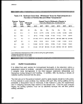 Section 403 Procedural and Monitoring Guidance
It is recommended that triplicate analyses be conducted on 1 of every 20 samples, or on
1 sample per batch if fewer than 20 samples are analyzed. It is recommended that the
analytical balance, drying oven, and temperature bath be inspected daily and calibrated
at least once per week.
4.4.5 Statistical Design Considerations
Statistical strategies may mitigate the high costs of collecting sufficient quantities of
sediment. Power analyses considering the strategy of compositing samples can often
lead to a cost-effective monitoring design strategy.
Composite Sampling
Composite sediment sampling consists of mixing samples from two or more replications
collected at a particular location at different times or at different locations at the same
time. The analysis of a composite sample provides an estimate of.an average
contaminant concentration for the locations composing the composite sample.
Advantages of the composite sampling strategy are:
• It provides a cost-effective strategy when individual analyses are expensive.
• It results in a more efficient estimate of the mean at specified sampling
locations.
Because of the reduced sample variance, composite sampling results in a considerable
increase in statistical power. If the primary objective of a monitoring program is to
determine differences in grain size between sampling locations, composite sampling is
an appropriate strategy.
Space-bulking consists of sampling from several locations and combining sediment
samples into one or more composite samples. Time-bulking involves taking multiple
samples over time from a single location and compositing these samples. Space- and
time-bulking strategies should be used judiciously since significant information
concerning spatial and temporal heterogeneity may be lost. The adoption of composite
strategies will depend on the objectives of individual monitoring programs.
Statistical Power
Statistical power increases with an increase in the number of sediment subsamples in
each replicate composite sample (USEPA, 1987d). However, with the addition of
successive subsamples to each composite, a diminished return of statistical power
exists. For composites of greater than 10 replications, the increase of power is
negligible given typical levels of data variability.
101
image:
Section 403 Procedural and Monitoring Guidance
It is recommended that triplicate analyses be conducted on 1 of every 20 samples, or on
1 sample per batch if fewer than 20 samples are analyzed. It is recommended that the
analytical balance, drying oven, and temperature bath be inspected daily and calibrated
at least once per week.
4.4.5 Statistical Design Considerations
Statistical strategies may mitigate the high costs of collecting sufficient quantities of
sediment. Power analyses considering the strategy of compositing samples can often
lead to a cost-effective monitoring design strategy.
Composite Sampling
Composite sediment sampling consists of mixing samples from two or more replications
collected at a particular location at different times or at different locations at the same
time. The analysis of a composite sample provides an estimate of.an average
contaminant concentration for the locations composing the composite sample.
Advantages of the composite sampling strategy are:
• It provides a cost-effective strategy when individual analyses are expensive.
• It results in a more efficient estimate of the mean at specified sampling
locations.
Because of the reduced sample variance, composite sampling results in a considerable
increase in statistical power. If the primary objective of a monitoring program is to
determine differences in grain size between sampling locations, composite sampling is
an appropriate strategy.
Space-bulking consists of sampling from several locations and combining sediment
samples into one or more composite samples. Time-bulking involves taking multiple
samples over time from a single location and compositing these samples. Space- and
time-bulking strategies should be used judiciously since significant information
concerning spatial and temporal heterogeneity may be lost. The adoption of composite
strategies will depend on the objectives of individual monitoring programs.
Statistical Power
Statistical power increases with an increase in the number of sediment subsamples in
each replicate composite sample (USEPA, 1987d). However, with the addition of
successive subsamples to each composite, a diminished return of statistical power
exists. For composites of greater than 10 replications, the increase of power is
negligible given typical levels of data variability.
101
image:
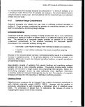 Methods
To improve the power of a statistical test, while keeping the significance level constant,
the sample size should be increased. Because of constraints in cost and time imposed
by the monitoring program, however, this option may not be available. Power analyses
have shown that for a fixed level of sampling effort, a monitoring program's power is
generally increased by collecting more replicates at fewer locations. The number and
distribution of sampling locations required to evaluate the effectiveness of the monitoring
program will depend on the size and complexity of the discharge and the surrounding
environment.
4.4.6
Use of Data
Results from sediment chemical monitoring can be normalized according to sediment
characteristics to account for some of the variability found in bioaccumulation rates.
Likewise, grain size information may explain the temporal and spatial variability in
biological assemblages. These results may be used to monitor rates of change
following the beginning of discharge, to evaluate the condition of benthic habitats, and to
assist in providing early warnings of potential impacts on the marine ecosystem.
The singular use of sediment grain size to assess the condition of the benthic habitat or
to guide the decision-making process is not recommended. The data collected from
monitoring the physical characteristics of sediments should be used in conjunction with
those collected from chemical and biological monitoring. Subsequent analyses of health
risks to human populations and ecological risks to benthic individuals, populations, and
communities may be performed. Sediment grain size provides evidence essential in the
evaluation of spatial and temporal effects of ocean discharges.
4.4.7 Summary and Recommendations
Rationale
• The objective of monitoring the physical characteristics of sediments is to
detect and describe spatial and temporal changes in sediment grain size.
• Results may be used to monitor rates of recovery following environmental
interventions, to evaluate the condition of benthic habitats, and to assist in
providing early warnings of discharge impacts to the surrounding ecosystem.
Monitoring Design Considerations
• It is recommended that the types of sampling gear and the location and
timing of sample collection be consistent to allow for comparisons among
studies.
• Collection of undisturbed sediment requires that the sampler:
- create a minimal bow wake when descending;
102
image:
Methods
To improve the power of a statistical test, while keeping the significance level constant,
the sample size should be increased. Because of constraints in cost and time imposed
by the monitoring program, however, this option may not be available. Power analyses
have shown that for a fixed level of sampling effort, a monitoring program's power is
generally increased by collecting more replicates at fewer locations. The number and
distribution of sampling locations required to evaluate the effectiveness of the monitoring
program will depend on the size and complexity of the discharge and the surrounding
environment.
4.4.6
Use of Data
Results from sediment chemical monitoring can be normalized according to sediment
characteristics to account for some of the variability found in bioaccumulation rates.
Likewise, grain size information may explain the temporal and spatial variability in
biological assemblages. These results may be used to monitor rates of change
following the beginning of discharge, to evaluate the condition of benthic habitats, and to
assist in providing early warnings of potential impacts on the marine ecosystem.
The singular use of sediment grain size to assess the condition of the benthic habitat or
to guide the decision-making process is not recommended. The data collected from
monitoring the physical characteristics of sediments should be used in conjunction with
those collected from chemical and biological monitoring. Subsequent analyses of health
risks to human populations and ecological risks to benthic individuals, populations, and
communities may be performed. Sediment grain size provides evidence essential in the
evaluation of spatial and temporal effects of ocean discharges.
4.4.7 Summary and Recommendations
Rationale
• The objective of monitoring the physical characteristics of sediments is to
detect and describe spatial and temporal changes in sediment grain size.
• Results may be used to monitor rates of recovery following environmental
interventions, to evaluate the condition of benthic habitats, and to assist in
providing early warnings of discharge impacts to the surrounding ecosystem.
Monitoring Design Considerations
• It is recommended that the types of sampling gear and the location and
timing of sample collection be consistent to allow for comparisons among
studies.
• Collection of undisturbed sediment requires that the sampler:
- create a minimal bow wake when descending;
102
image:
 Section 403 Procedural and Monitoring Guidance
- form a leakproof seal when the sediment sample is taken;
- prevent winnowing and excessive sample disturbance when ascending; and
- allow easy access to the sample surface in order that undisturbed
subsamples may be taken.
• Analysis of the upper 2 cm is advised in order to examine recent depositional
events.
• Penetration well below the desired sampling depth is preferred to prevent
sample disturbance as the device closes.
Analytical Methods Considerations
• Because true and apparent distributions differ, detailed comparisons between
samples analyzed by different methods are questionable. It is therefore
desirable that all samples within each study and among different studies in
the study area be analyzed using only one method.
QA/QC Considerations
• Laboratory homogenization should be conducted even if samples were
homogenized in the field.
• It is recommended that triplicate analyses be conducted on 1 of every 20
samples, or on 1 sample per batch if fewer than 20 samples are analyzed.
• It is recommended that the analytical balance, drying oven, and temperature
bath be inspected daily and calibrated at least once per week.
Statistical Design Considerations
• Compositing sediment sampling consists of mixing samples from two or more
replications collected at a particular location and time period.
• Space-bulking (combining composites from several locations) and
time-bulking (combining several composites over time from one location)
strategies should be used judiciously since information concerning spatial
and temporal heterogeneity may be lost.
• Power analyses have shown that for a fixed level of sampling effort, the
power of a monitoring program is generally increased by collecting more
replicates at fewer locations.
103
image:
Section 403 Procedural and Monitoring Guidance
- form a leakproof seal when the sediment sample is taken;
- prevent winnowing and excessive sample disturbance when ascending; and
- allow easy access to the sample surface in order that undisturbed
subsamples may be taken.
• Analysis of the upper 2 cm is advised in order to examine recent depositional
events.
• Penetration well below the desired sampling depth is preferred to prevent
sample disturbance as the device closes.
Analytical Methods Considerations
• Because true and apparent distributions differ, detailed comparisons between
samples analyzed by different methods are questionable. It is therefore
desirable that all samples within each study and among different studies in
the study area be analyzed using only one method.
QA/QC Considerations
• Laboratory homogenization should be conducted even if samples were
homogenized in the field.
• It is recommended that triplicate analyses be conducted on 1 of every 20
samples, or on 1 sample per batch if fewer than 20 samples are analyzed.
• It is recommended that the analytical balance, drying oven, and temperature
bath be inspected daily and calibrated at least once per week.
Statistical Design Considerations
• Compositing sediment sampling consists of mixing samples from two or more
replications collected at a particular location and time period.
• Space-bulking (combining composites from several locations) and
time-bulking (combining several composites over time from one location)
strategies should be used judiciously since information concerning spatial
and temporal heterogeneity may be lost.
• Power analyses have shown that for a fixed level of sampling effort, the
power of a monitoring program is generally increased by collecting more
replicates at fewer locations.
103
image:
 Methods
Use ofJData
The singular use of sediment grain size monitoring to assess the condition of
the benthic habitat or to guide the decision-making process is not
recommended; data collected from monitoring the physical characteristics of
sediments should be used in conjunction with those collected from chemical
and biological monitoring.
Results from sediment grain size monitoring can be used to normalize
sediment pollutant results to account for some of the variability found in
bioaccumulation rates.
Grain size information may explain the temporal and spatial variability in
biological assemblages.
104
image:
Methods
Use ofJData
The singular use of sediment grain size monitoring to assess the condition of
the benthic habitat or to guide the decision-making process is not
recommended; data collected from monitoring the physical characteristics of
sediments should be used in conjunction with those collected from chemical
and biological monitoring.
Results from sediment grain size monitoring can be used to normalize
sediment pollutant results to account for some of the variability found in
bioaccumulation rates.
Grain size information may explain the temporal and spatial variability in
biological assemblages.
104
image:
 Section 403 Procedural and Monitoring Quittance
4.5
BENTHIC COMMUNITY STRUCTURE
The objective of benthic monitoring is the detection and description of spatial and
temporal changes in community structure and function. The results can assess the
condition or "health" of berithic habitats and monitor the rates of recovery following
environmental or human disturbances. Benthic fauna also represent a significant food
source for many marine organisms, thereby providing an early warning of potential
impacts on the marine ecosystem.
Benthic habitats may be broadly divided into hard- and soft-bottom substrates. Those
habitats with soft-bottom substrates (e.g., sand, silt, mud) are composed of a significant
benthic biological community known as infauna. This community consists of organisms
that burrow into the substratum itself. The communities found over hard-bottom
substrata such as coral reefs, rocky subtidal areas, and "live bottom" sponge/gorgonian
habitats are referred to as epifauna. There are numerous species of polychaete worms,
pelecypod molluscs, and sponges capable of penetrating the substratum; however, the
majority of the community is found on top of the substratum. The latter hard-bottom or
"live bottom" communities of dense sessile epifauna are valuable because they attract
commercially and ecologically important species of fish (Darcy and Gutherz, 1984).
4.5.1
Rationale
Of the 10 guidelines used to determine unreasonable degradation and no irreparable
harm, the following can be assessed by evaluating the benthic community structure:
• Composition and vulnerability of potentially exposed biological communities and
• Importance of the receiving water area to the surrounding biological
community.
Monitoring the abundance of individual benthic organisms is a widely-accepted means
of measuring the condition off the benthic habitat (Bilyard, 1987). Benthic organisms are
exceptional indicators of benfhic conditions since:
• They are usually sedentary; consequently, observed effects are in response
to local environmental conditions, and their relative longevity of up to a year
or more provides a level of consistency to data gathered.
• They are sensitive to habitat disturbance; communities undergo dramatic
changes in species composition and abundance in response to
environmental perturbations.
• They often mediate the transfer of nutrients and toxic substances in the
ecosystem (via bioturbation and as important prey organisms).
105
image:
Section 403 Procedural and Monitoring Quittance
4.5
BENTHIC COMMUNITY STRUCTURE
The objective of benthic monitoring is the detection and description of spatial and
temporal changes in community structure and function. The results can assess the
condition or "health" of berithic habitats and monitor the rates of recovery following
environmental or human disturbances. Benthic fauna also represent a significant food
source for many marine organisms, thereby providing an early warning of potential
impacts on the marine ecosystem.
Benthic habitats may be broadly divided into hard- and soft-bottom substrates. Those
habitats with soft-bottom substrates (e.g., sand, silt, mud) are composed of a significant
benthic biological community known as infauna. This community consists of organisms
that burrow into the substratum itself. The communities found over hard-bottom
substrata such as coral reefs, rocky subtidal areas, and "live bottom" sponge/gorgonian
habitats are referred to as epifauna. There are numerous species of polychaete worms,
pelecypod molluscs, and sponges capable of penetrating the substratum; however, the
majority of the community is found on top of the substratum. The latter hard-bottom or
"live bottom" communities of dense sessile epifauna are valuable because they attract
commercially and ecologically important species of fish (Darcy and Gutherz, 1984).
4.5.1
Rationale
Of the 10 guidelines used to determine unreasonable degradation and no irreparable
harm, the following can be assessed by evaluating the benthic community structure:
• Composition and vulnerability of potentially exposed biological communities and
• Importance of the receiving water area to the surrounding biological
community.
Monitoring the abundance of individual benthic organisms is a widely-accepted means
of measuring the condition off the benthic habitat (Bilyard, 1987). Benthic organisms are
exceptional indicators of benfhic conditions since:
• They are usually sedentary; consequently, observed effects are in response
to local environmental conditions, and their relative longevity of up to a year
or more provides a level of consistency to data gathered.
• They are sensitive to habitat disturbance; communities undergo dramatic
changes in species composition and abundance in response to
environmental perturbations.
• They often mediate the transfer of nutrients and toxic substances in the
ecosystem (via bioturbation and as important prey organisms).
105
image:
 Methods
Furthermore, monitoring benthic organisms is one of a handful of methods that provide
in situ measures of biotic health and habitat quality. The assessment of benthic infaunal
and epifaunal community structure is a powerful tool in the evaluation of spatial and
temporal effects of anthropogenic and natural disturbance.
4.5.2 Monitoring Design Considerations
The level of effort required to assess benthic community structure is relatively high. A
field survey is required to record and/or collect organisms, and sorting, identifying, and
enumerating specimens require labor-intensive and generally expensive processes.
Evaluations of benthic community structure and function may also be costly and
time-consuming.
The results of benthic monitoring programs can vary substantially depending on the
objectives and corresponding design specifications. The characteristics that are
primarily responsible for the variability in the results are :
• Type of surveying and/or sampling gear;
• Sample sorting and/or data analysis protocols;
• Level of taxonomy; and
• Location and timing of sample collection.
The object is to standardize the measurement techniques at all stages of the 403
monitoring program to ensure that the data can be intercompared. Efforts should be
made to try to match new monitoring data with historical data, but differences in
techniques and sampling gear should be avoided. Historical data may be used only to
note trends in the benthic fauna and, in particular, to follow any succession occurring as
a result of increases in pollution.
Analyses of power-cost efficiencies are essential in selecting the appropriate survey
technique and/or sampling gear and sample/data processing protocols. Ferraro et al.
(1989) provide an example of power-cost analysis.
Different techniques are available for surveying and sampling organisms in hard- or
soft-bottom habitats. Since these protocols will influence all subsequent laboratory and
data analyses, it is essential that benthic samples be collected using acceptable and
standardized techniques. Furthermore, samples of sediments and benthic organisms
should be collected concurrently to mitigate the costs of field sampling and to permit
sound correlation and multivariate analyses (see Sediment Chemistry). Therefore, it is
recommended that soft-bottom sampling devices also be suitable for sampling the
sediment (Table 4-18).
106
image:
Methods
Furthermore, monitoring benthic organisms is one of a handful of methods that provide
in situ measures of biotic health and habitat quality. The assessment of benthic infaunal
and epifaunal community structure is a powerful tool in the evaluation of spatial and
temporal effects of anthropogenic and natural disturbance.
4.5.2 Monitoring Design Considerations
The level of effort required to assess benthic community structure is relatively high. A
field survey is required to record and/or collect organisms, and sorting, identifying, and
enumerating specimens require labor-intensive and generally expensive processes.
Evaluations of benthic community structure and function may also be costly and
time-consuming.
The results of benthic monitoring programs can vary substantially depending on the
objectives and corresponding design specifications. The characteristics that are
primarily responsible for the variability in the results are :
• Type of surveying and/or sampling gear;
• Sample sorting and/or data analysis protocols;
• Level of taxonomy; and
• Location and timing of sample collection.
The object is to standardize the measurement techniques at all stages of the 403
monitoring program to ensure that the data can be intercompared. Efforts should be
made to try to match new monitoring data with historical data, but differences in
techniques and sampling gear should be avoided. Historical data may be used only to
note trends in the benthic fauna and, in particular, to follow any succession occurring as
a result of increases in pollution.
Analyses of power-cost efficiencies are essential in selecting the appropriate survey
technique and/or sampling gear and sample/data processing protocols. Ferraro et al.
(1989) provide an example of power-cost analysis.
Different techniques are available for surveying and sampling organisms in hard- or
soft-bottom habitats. Since these protocols will influence all subsequent laboratory and
data analyses, it is essential that benthic samples be collected using acceptable and
standardized techniques. Furthermore, samples of sediments and benthic organisms
should be collected concurrently to mitigate the costs of field sampling and to permit
sound correlation and multivariate analyses (see Sediment Chemistry). Therefore, it is
recommended that soft-bottom sampling devices also be suitable for sampling the
sediment (Table 4-18).
106
image:
 Section 403 Procedural and Monitoring Guidance
Hard-Bottom Habitat Surveys
In hard-bottom habitats, benthic surveys are used to document the relative cover of
sessile organisms on the substratum and species distributions. Depending on weather
and water conditions, these surveys can be performed by divers, or remotely operated
vehicles (ROVs) or submarines can be used (Gamble, 1984; Holme, 1984). Specimens
and sediment samples can then be directly collected by the diver or submarine to
provide vouchers for positive taxa identification and for pathobiological or chemical
analyses.
Types of Surveys
Numerous methods and techniques have been examined and compared to quantify
hard-bottom community structure, particularly on coral reefs. These include simple line
transects, quadrats, and plotless distance or nearest neighbor techniques. The data
collected on species and organism coverage of the substratum allow calculations of
species diversity, abundances, richness, and percent live tissue. Both randomly placed
and "permanent" sites (marked by pins cemented into the substratum to allow accurate
monitoring of the same site over time) have been used; each suffers from its own biases
for statistical analyses. Each technique also presents problems in quantification and
interpretation of data (see Loya, 1978; Gamble, 1984; Brown, 1988). Results of
comparative studies indicate that:
• Although line transects are popular, they are not really very helpful unless
multiple, closely-spaced 10-meter transects along same-depth contours are
evaluated (Dustan and Halas, 1987).
• The linear point intercept method appears to be quite efficient and yields
species abundance estimates similar to the true habitat (Ohlhorst et al., 1988).
• One-meter-square mapped quadrats provide good data for colony counts and
estimates of percent coverage (Weinberg, 1981), but 4-meter-square
quadrats are better for detecting rarer species.
• Photographed belt quadrats (1x10 meters-square) may provide the most
information, although clear water conditions and long analysis time are
necessary (Dodge et al., 1982).
Examples of line transects include a straight weighted line stretched over the
substratum, with the species and lengths of live tissue underlying the line measured by
tape, or the modification by Porter (1972), in which a chain of uniform links is placed
over the corals and the number of links is counted and converted to area of live tissue
cover. Rogers et al. (1983) used the ratio of the straight line to the length of chain
required to cover the same distance as an estimate of the topographic relief of the
substratum. Photogrammetry, in which still photographs are made of continuous areas
under the transect line, provides a permanent record that can be quantified by computer
107
image:
Section 403 Procedural and Monitoring Guidance
Hard-Bottom Habitat Surveys
In hard-bottom habitats, benthic surveys are used to document the relative cover of
sessile organisms on the substratum and species distributions. Depending on weather
and water conditions, these surveys can be performed by divers, or remotely operated
vehicles (ROVs) or submarines can be used (Gamble, 1984; Holme, 1984). Specimens
and sediment samples can then be directly collected by the diver or submarine to
provide vouchers for positive taxa identification and for pathobiological or chemical
analyses.
Types of Surveys
Numerous methods and techniques have been examined and compared to quantify
hard-bottom community structure, particularly on coral reefs. These include simple line
transects, quadrats, and plotless distance or nearest neighbor techniques. The data
collected on species and organism coverage of the substratum allow calculations of
species diversity, abundances, richness, and percent live tissue. Both randomly placed
and "permanent" sites (marked by pins cemented into the substratum to allow accurate
monitoring of the same site over time) have been used; each suffers from its own biases
for statistical analyses. Each technique also presents problems in quantification and
interpretation of data (see Loya, 1978; Gamble, 1984; Brown, 1988). Results of
comparative studies indicate that:
• Although line transects are popular, they are not really very helpful unless
multiple, closely-spaced 10-meter transects along same-depth contours are
evaluated (Dustan and Halas, 1987).
• The linear point intercept method appears to be quite efficient and yields
species abundance estimates similar to the true habitat (Ohlhorst et al., 1988).
• One-meter-square mapped quadrats provide good data for colony counts and
estimates of percent coverage (Weinberg, 1981), but 4-meter-square
quadrats are better for detecting rarer species.
• Photographed belt quadrats (1x10 meters-square) may provide the most
information, although clear water conditions and long analysis time are
necessary (Dodge et al., 1982).
Examples of line transects include a straight weighted line stretched over the
substratum, with the species and lengths of live tissue underlying the line measured by
tape, or the modification by Porter (1972), in which a chain of uniform links is placed
over the corals and the number of links is counted and converted to area of live tissue
cover. Rogers et al. (1983) used the ratio of the straight line to the length of chain
required to cover the same distance as an estimate of the topographic relief of the
substratum. Photogrammetry, in which still photographs are made of continuous areas
under the transect line, provides a permanent record that can be quantified by computer
107
image:
 Methods
digitizing techniques (Bohnsack, 1979; Dodge et al., 1982; White and Porter, 1985).
Further developments in this area include computer automation for analyses and using
underwater video to record along transects. Although the latter technique is faster and
easier to perform either by divers or ROVs, problems with quantifying the observations
have not been worked out. However, video does provide an important visual record for
assessing changes overtime (Holme, 1984; Rogers, 1988).
For all of these methods, a number of trade-offs must be considered. Since most of this
work must be performed by divers, diver safety is of the utmost importance, including
the amount of bottom time available, the skill levels of the divers, and the type and
degree of pollution that may be encountered. The types and amounts of information
required for each species, as well as the length of time of the survey, will also affect the
study design and techniques to be used. For many hard-bottom areas, there may not
be one "best" method for monitoring and sampling the epifauna. Thus, two or more
methods may be required to provide an adequate assessment of benthic community
structure over time (see, for example, Dodge et al., 1982; Holme and Mclntyre, 1984;
Dayton, 1985; Witman, 1985; Rogers, 1988; Phillips etal., 1990).
Soft-Bottom Sampling Devices
In soft-bottom habitats, several types of devices can be used to collect benthic
macroinvertebrate samples from the sediment: trawls, dredges, grabs, and box corers
(Mclntyre et al., 1984). The organisms collected in each sample are then identified and
species distributions determined. Most of these devices sample the benthos in a unique
manner. Accordingly, conducting comparisons between data collected using different
devices is inadvisable. The same area and volume of sediment should be sampled
since different species of benthic infaunal macroinvertebrates exhibit different horizontal
and vertical distributions (Elliot, 1971).
Collection of an acceptable sediment sample for infaunal analyses requires that the
sampler:
• Create a minimal bow wake when descending;
• Form a leakproof seal when the sediment sample is taken;
• Prevent winnowing and excessive sample disturbance when ascending; and
• Allow easy access to the sample surface in order that undisturbed
subsamples may be taken.
Penetration well below the desired sampling depth is preferred to prevent sample
disturbance as the device closes. It is optimal to use a sampler that has a means of
weight adjustment to allow modification of penetration depths.
108
image:
Methods
digitizing techniques (Bohnsack, 1979; Dodge et al., 1982; White and Porter, 1985).
Further developments in this area include computer automation for analyses and using
underwater video to record along transects. Although the latter technique is faster and
easier to perform either by divers or ROVs, problems with quantifying the observations
have not been worked out. However, video does provide an important visual record for
assessing changes overtime (Holme, 1984; Rogers, 1988).
For all of these methods, a number of trade-offs must be considered. Since most of this
work must be performed by divers, diver safety is of the utmost importance, including
the amount of bottom time available, the skill levels of the divers, and the type and
degree of pollution that may be encountered. The types and amounts of information
required for each species, as well as the length of time of the survey, will also affect the
study design and techniques to be used. For many hard-bottom areas, there may not
be one "best" method for monitoring and sampling the epifauna. Thus, two or more
methods may be required to provide an adequate assessment of benthic community
structure over time (see, for example, Dodge et al., 1982; Holme and Mclntyre, 1984;
Dayton, 1985; Witman, 1985; Rogers, 1988; Phillips etal., 1990).
Soft-Bottom Sampling Devices
In soft-bottom habitats, several types of devices can be used to collect benthic
macroinvertebrate samples from the sediment: trawls, dredges, grabs, and box corers
(Mclntyre et al., 1984). The organisms collected in each sample are then identified and
species distributions determined. Most of these devices sample the benthos in a unique
manner. Accordingly, conducting comparisons between data collected using different
devices is inadvisable. The same area and volume of sediment should be sampled
since different species of benthic infaunal macroinvertebrates exhibit different horizontal
and vertical distributions (Elliot, 1971).
Collection of an acceptable sediment sample for infaunal analyses requires that the
sampler:
• Create a minimal bow wake when descending;
• Form a leakproof seal when the sediment sample is taken;
• Prevent winnowing and excessive sample disturbance when ascending; and
• Allow easy access to the sample surface in order that undisturbed
subsamples may be taken.
Penetration well below the desired sampling depth is preferred to prevent sample
disturbance as the device closes. It is optimal to use a sampler that has a means of
weight adjustment to allow modification of penetration depths.
108
image:
 Section 403 Procedural and Monitoring Guidance
Trawls and Dredges
Trawls and dredges usually collect organisms over a variable and relatively large area
(USEPA, 1986-1991; Fredette et al.( 1989). The data collected using these devices are
qualitative since consistent and reproducible sampling of a consistent benthic area is not
possible. Their design and use preclude the collection of infaunal organisms at
sediment depths greater than a few centimeters. Although trawls and dredges may be
used to collect samples of either infaunal or epifaunal specimens for
chemical/pathobiological studies, the specimens can be damaged by physical scrapes
or breakage during this type of collection and adherent sand or silt particles could
interfere with these analyses. However, these devices are suitable for reconnaissance
of potential sampling sites.
Grab Samplers
Grab samplers are capable of consistent sampling of bottom habitats; depending on the
size of the device, areas from 0.02 to 0.5 m2 and depths ranging from 5 to 15 cm may
be sampled. Limitations of grab samplers include:
• Variability among samples in penetration depth, depending on sediment
properties;
• Oblique angles of penetration, which result in varying penetration depths
within a sample; and
• Folding of the sample, which results in the inability to section the sample and
the loss of information concerning the vertical structure in the sediments.
However, the careful use of these devices will provide quantitative data. Grab samplers
are the tools of choice for a number of marine monitoring programs because of their
ability to provide quantitative data at a relatively low cost. (Fredette et al., 1989;
USEPA, 1986-1991).
Core Samplers
Core samplers use a surrounding frame to ensure vertical entry; vertical sectioning of
the sample is possible (USEEPA, 1986-1991). These devices are capable of maximum
penetration depths of 15 cm and may collect volumes 5 to 10 times that of grab
samplers. Limitations of box corers include :
• Large size and weight, which require the use of cranes or winches and a
large vessel for deployment;
• Higher construction expenses; and
• Lack of calibration studies to permit comparisons to grab samples.
109
image:
Section 403 Procedural and Monitoring Guidance
Trawls and Dredges
Trawls and dredges usually collect organisms over a variable and relatively large area
(USEPA, 1986-1991; Fredette et al.( 1989). The data collected using these devices are
qualitative since consistent and reproducible sampling of a consistent benthic area is not
possible. Their design and use preclude the collection of infaunal organisms at
sediment depths greater than a few centimeters. Although trawls and dredges may be
used to collect samples of either infaunal or epifaunal specimens for
chemical/pathobiological studies, the specimens can be damaged by physical scrapes
or breakage during this type of collection and adherent sand or silt particles could
interfere with these analyses. However, these devices are suitable for reconnaissance
of potential sampling sites.
Grab Samplers
Grab samplers are capable of consistent sampling of bottom habitats; depending on the
size of the device, areas from 0.02 to 0.5 m2 and depths ranging from 5 to 15 cm may
be sampled. Limitations of grab samplers include:
• Variability among samples in penetration depth, depending on sediment
properties;
• Oblique angles of penetration, which result in varying penetration depths
within a sample; and
• Folding of the sample, which results in the inability to section the sample and
the loss of information concerning the vertical structure in the sediments.
However, the careful use of these devices will provide quantitative data. Grab samplers
are the tools of choice for a number of marine monitoring programs because of their
ability to provide quantitative data at a relatively low cost. (Fredette et al., 1989;
USEPA, 1986-1991).
Core Samplers
Core samplers use a surrounding frame to ensure vertical entry; vertical sectioning of
the sample is possible (USEEPA, 1986-1991). These devices are capable of maximum
penetration depths of 15 cm and may collect volumes 5 to 10 times that of grab
samplers. Limitations of box corers include :
• Large size and weight, which require the use of cranes or winches and a
large vessel for deployment;
• Higher construction expenses; and
• Lack of calibration studies to permit comparisons to grab samples.
109
image:
 Methods
The Hessler-Sandia box corer uses dividers to section the core into subsections,
facilitating subsampling of the core.
Box corers are recognized as the tools of choice for maximum accuracy and precision
when sampling soft-bottom habitats. Smaller corers may also be handled by divers.
Suction Samplers
In situ suction devices use the flow of water to collect sediments and benthic organisms
(Eleftheriou and Holme, 1984). An open-ended suction tube draws sediments and
organisms into the flow of water, and the organisms are trapped in a sieve or mesh bag
at the end of the tube. Limitations of suction devices include :
• Little control of the volume of sediment collected;
• Collection of animals from surrounding sediments, therefore inflating
abundances; and
• Abrading organisms during collection, making identification even more
difficult.
Fleishack et al. (1985) propose modifications to suction samplers that overcome some
of these limitations. Although samplers can be operated remotely, most must be
controlled by divers. Diver-operated collections are restricted to scuba depths and
conditions that permit safe diving (e.g., relatively calm waters, reasonable visibility).
This restriction limits their use in monitoring programs.
Sediment Profiling Camera
The sediment profiling camera is a unique tool that allows vertical, in situ imaging of the
water-sediment interface. Photographs of biological activity may be made at a
maximum depth of 18 cm; however, the penetration depth of the viewing prism may be
limited because of the physical characteristics of the sediment (i.e., penetration depths
are greater in silt than in sand).
The sediment profiling camera system can give measurements of organism tube
density, thickness of the pelletal layer, and infauna present in the image area (Rhoads
and Germano, 1982). Although this tool provides qualitative information concerning
benthos activity, the sediment profiling camera system cannot provide quantitative
information on species diversity, abundance, and biomass. Information concerning
species composition cannot be gained using this tool. Consequently, characterizations
of the benthic community structure cannot be made from the data taken from these
images.
110
image:
Methods
The Hessler-Sandia box corer uses dividers to section the core into subsections,
facilitating subsampling of the core.
Box corers are recognized as the tools of choice for maximum accuracy and precision
when sampling soft-bottom habitats. Smaller corers may also be handled by divers.
Suction Samplers
In situ suction devices use the flow of water to collect sediments and benthic organisms
(Eleftheriou and Holme, 1984). An open-ended suction tube draws sediments and
organisms into the flow of water, and the organisms are trapped in a sieve or mesh bag
at the end of the tube. Limitations of suction devices include :
• Little control of the volume of sediment collected;
• Collection of animals from surrounding sediments, therefore inflating
abundances; and
• Abrading organisms during collection, making identification even more
difficult.
Fleishack et al. (1985) propose modifications to suction samplers that overcome some
of these limitations. Although samplers can be operated remotely, most must be
controlled by divers. Diver-operated collections are restricted to scuba depths and
conditions that permit safe diving (e.g., relatively calm waters, reasonable visibility).
This restriction limits their use in monitoring programs.
Sediment Profiling Camera
The sediment profiling camera is a unique tool that allows vertical, in situ imaging of the
water-sediment interface. Photographs of biological activity may be made at a
maximum depth of 18 cm; however, the penetration depth of the viewing prism may be
limited because of the physical characteristics of the sediment (i.e., penetration depths
are greater in silt than in sand).
The sediment profiling camera system can give measurements of organism tube
density, thickness of the pelletal layer, and infauna present in the image area (Rhoads
and Germano, 1982). Although this tool provides qualitative information concerning
benthos activity, the sediment profiling camera system cannot provide quantitative
information on species diversity, abundance, and biomass. Information concerning
species composition cannot be gained using this tool. Consequently, characterizations
of the benthic community structure cannot be made from the data taken from these
images.
110
image:
 Section 403 Procedural and Monitoring Guidance
The sediment profiling camera is not recommended for the collection of benthic
community structure data; however, it is an effective reconnaissance tool. Delineation of
physically similar sampling sites may be determined through the use of this tool, aiding
in the selection of sampling stations. Ground-truthing of these images by means of
laboratory analyses of collected material is highly recommended.
If quantitative analyses of infaunal benthic community structure are required, a grab or
core sampler is recommended. Either of these sampling devices permits adequate
sampling of both sediment and benthic infaunal communities with one sampling device.
Sampling Area
The numerous species of benthic macroinvertebrates have varying scales of spatial
distribution both horizontally and vertically (Elliot, 1971; Livingston et at., 1976; Loya,
1978; Downing, 1979). Field and laboratory costs increase with increasing sample size;
therefore, the determination of the optimal sample size must consider spatial and
temporal scales, as well as statistical power. Preliminary community surveys should be
undertaken to determine the most appropriate technique for the site(s) and the optimal
balance between the types of information and/or samples needed and the time available
for each survey/sampling session and subsequent analyses. In particular, the limitations
and requirements of the biological indices used in the data analyses to determine
community structure must be carefully considered to set the optimal sampling area.
Selection of Sampling Period
Benthic infauna assemblages are dynamic; the most common temporal patterns
observed in benthic communities are those associated with seasonal changes.
Seasonal variation in benthic assemblages may be due to changes in physical,
chemical, and/or biological parameters, e.g., temperature, light transmissivity, dissolved
oxygen, predation, recruitment, etc.
Given the seasonal variation characteristic of benthic assemblages in general, it is
recommended that direct comparisons between samples collected during different
seasons be avoided. Studies investigating interannual variation in the characteristics of
benthic communities should be conducted during the same season (preferably the same
month) each year.
Data Collection Protocols
For both hard and soft bottoms, the species present and numbers of individuals need to
be determined to characterize the benthic community structure. During hard-bottom
surveys, this information may be collected by the diver (recording the data on an
underwater slate or waterproof paper, on which the format for either transect or quadrat
information has been preprinted to facilitate data recording), or it may be derived from
photographs (examined by light microscopy or computer scanning techniques) at a later
111
image:
Section 403 Procedural and Monitoring Guidance
The sediment profiling camera is not recommended for the collection of benthic
community structure data; however, it is an effective reconnaissance tool. Delineation of
physically similar sampling sites may be determined through the use of this tool, aiding
in the selection of sampling stations. Ground-truthing of these images by means of
laboratory analyses of collected material is highly recommended.
If quantitative analyses of infaunal benthic community structure are required, a grab or
core sampler is recommended. Either of these sampling devices permits adequate
sampling of both sediment and benthic infaunal communities with one sampling device.
Sampling Area
The numerous species of benthic macroinvertebrates have varying scales of spatial
distribution both horizontally and vertically (Elliot, 1971; Livingston et at., 1976; Loya,
1978; Downing, 1979). Field and laboratory costs increase with increasing sample size;
therefore, the determination of the optimal sample size must consider spatial and
temporal scales, as well as statistical power. Preliminary community surveys should be
undertaken to determine the most appropriate technique for the site(s) and the optimal
balance between the types of information and/or samples needed and the time available
for each survey/sampling session and subsequent analyses. In particular, the limitations
and requirements of the biological indices used in the data analyses to determine
community structure must be carefully considered to set the optimal sampling area.
Selection of Sampling Period
Benthic infauna assemblages are dynamic; the most common temporal patterns
observed in benthic communities are those associated with seasonal changes.
Seasonal variation in benthic assemblages may be due to changes in physical,
chemical, and/or biological parameters, e.g., temperature, light transmissivity, dissolved
oxygen, predation, recruitment, etc.
Given the seasonal variation characteristic of benthic assemblages in general, it is
recommended that direct comparisons between samples collected during different
seasons be avoided. Studies investigating interannual variation in the characteristics of
benthic communities should be conducted during the same season (preferably the same
month) each year.
Data Collection Protocols
For both hard and soft bottoms, the species present and numbers of individuals need to
be determined to characterize the benthic community structure. During hard-bottom
surveys, this information may be collected by the diver (recording the data on an
underwater slate or waterproof paper, on which the format for either transect or quadrat
information has been preprinted to facilitate data recording), or it may be derived from
photographs (examined by light microscopy or computer scanning techniques) at a later
111
image:
 Methods
date. The organisms collected by grab or corer devices from soft bottoms must be
rinsed from the sediments, preserved, and sorted for identification and enumeration.
Several options must be considered when designing sorting protocols. To ensure
comparability between studies, a consistent set of sorting procedures is highly
recommended.
Sieving: Mesh Size and Location
The use of different sieve mesh sizes limits the comparability of results between marine
monitoring studies (Reish, 1959; Rees, 1984). The major advantage of using a smaller
mesh size is the retention of both juvenile and adult organisms as well as large- and
small-bodied taxa. The major disadvantage is the concomitant increased cost of sample
processing. For example, using a 0.5-mm mesh over a 1.00-mm mesh could increase
retention of total microfaunal organisms by 130-180 percent; however, costs for
processing the samples may increase as much as 200 percent (USEPA, 1986-1991).
It is recommended that a standard mesh size be selected for all monitoring studies. The
1.0-mm mesh size is commonly used in impact assessments, and the 0.5-mm mesh
size is sometimes used in recruitment studies. The issue of data comparability was
resolved by recommending sequential screening and analysis procedures (Becker and
Armstrong, 1988). By screening samples through both the 1.0- and 0.5-mm sieves, the
1.0-mm fraction could be analyzed separately and the data compared with other impact
studies. The data for the 0.5-mm fraction of the samples could then be combined to
yield information on the complete sample for comparison with other recruitment data.
Sieving can be done either aboard the survey vessel or on shore after the cruise.
Sieving occurs prior to fixation (sample preservation) aboard the vessel, whereas
waiting until after the cruise requires fixation prior to sieving. If inadequate
concentrations of fixative are added and deterioration or decomposition of organisms
occurs, there may be a significant detrimental modification of the sample. If large
numbers of samples are to be collected, field sieving reduces the sample volume
required for storage, as well as the modification/loss of data.
Use of Relaxants
The use of relaxants prior to sieving and fixation reduces the tendency of organisms to
distort their shape or autotomize, and consequently facilitates taxonomic identifications
and morphometric measurements (USEPA, 1986-1991). Complete organisms, having a
"natural" appearance, are easier to identify to a lower taxonomic group than are
distorted or fragmented specimens.
112
image:
Methods
date. The organisms collected by grab or corer devices from soft bottoms must be
rinsed from the sediments, preserved, and sorted for identification and enumeration.
Several options must be considered when designing sorting protocols. To ensure
comparability between studies, a consistent set of sorting procedures is highly
recommended.
Sieving: Mesh Size and Location
The use of different sieve mesh sizes limits the comparability of results between marine
monitoring studies (Reish, 1959; Rees, 1984). The major advantage of using a smaller
mesh size is the retention of both juvenile and adult organisms as well as large- and
small-bodied taxa. The major disadvantage is the concomitant increased cost of sample
processing. For example, using a 0.5-mm mesh over a 1.00-mm mesh could increase
retention of total microfaunal organisms by 130-180 percent; however, costs for
processing the samples may increase as much as 200 percent (USEPA, 1986-1991).
It is recommended that a standard mesh size be selected for all monitoring studies. The
1.0-mm mesh size is commonly used in impact assessments, and the 0.5-mm mesh
size is sometimes used in recruitment studies. The issue of data comparability was
resolved by recommending sequential screening and analysis procedures (Becker and
Armstrong, 1988). By screening samples through both the 1.0- and 0.5-mm sieves, the
1.0-mm fraction could be analyzed separately and the data compared with other impact
studies. The data for the 0.5-mm fraction of the samples could then be combined to
yield information on the complete sample for comparison with other recruitment data.
Sieving can be done either aboard the survey vessel or on shore after the cruise.
Sieving occurs prior to fixation (sample preservation) aboard the vessel, whereas
waiting until after the cruise requires fixation prior to sieving. If inadequate
concentrations of fixative are added and deterioration or decomposition of organisms
occurs, there may be a significant detrimental modification of the sample. If large
numbers of samples are to be collected, field sieving reduces the sample volume
required for storage, as well as the modification/loss of data.
Use of Relaxants
The use of relaxants prior to sieving and fixation reduces the tendency of organisms to
distort their shape or autotomize, and consequently facilitates taxonomic identifications
and morphometric measurements (USEPA, 1986-1991). Complete organisms, having a
"natural" appearance, are easier to identify to a lower taxonomic group than are
distorted or fragmented specimens.
112
image:
 Section 403 Procedural and Monitoring Guidance
The magnitude to which relaxants can influence taxonomic identification, thereby limiting
comparisons between monitoring studies, is unknown. It is not recommended that
comparisons be conducted between studies in which relaxants were used and those in
which they were not used.
Use of Stains
Vital stains—primarily rose bengal—are added to samples to facilitate sorting. The stain
colors most infauna, enhancing their contrast with background debris. Not all taxa stain
adequately, and some taxonomists have found that staining interferes with the
identification of certain taxa. Although staining may aid the sorting process, a proper
quality control program should ensure that sorting efficiency is maintained whether or
not a stain is used.
Level of Taxonomy
The necessity to identify organisms to the level of species has recently been questioned
(Warwick, 1986). The liabilities of identifying organisms to the species level include :
• Identifications may be inaccurate and imprecise (Ellis, 1985).
• Identifications are time-consuming and costly; costs can be reduced as much
as 30-50 percent by limiting identification of samples to higher taxonomic
groups (USEPA, 1986-1991).
Identifications to higher taxonomic groups can provide gross characterizations of benthic
assemblages and may be sufficient to meet program objectives concerning detection of
community responses to anthropogenic disturbance. Warwick (1986) contends that
detection of anthropogenic disturbances would be facilitated since these perturbations
affect community structure at taxonomic levels higher than the species level. Natural
disturbances, which generally affect community structure by species replacement, would
have little influence on analyses at higher taxonomic levels.
However, identification to higher taxonomic levels may sacrifice the potential wealth of
information available using species-level identification such as analyses of population
dynamics and productivity. Furthermore, it is generally regarded that species is the
taxon most susceptible to environmental stress; individuals tend to be replaced by
another species within the same genus before the genus is replaced (USEPA,
1986-1991).
The level of taxonomic identification will depend on monitoring program objectives,
sample size, study sites, analytical measure, and availability of trained taxonomists.
Data based on lower taxonomic levels can be grouped for future comparisons with
higher level taxa. It is strongly recommended that all samples identified only to higher
taxonomic levels be properly archived, since comparisons of lower taxonomic data may
113
image:
Section 403 Procedural and Monitoring Guidance
The magnitude to which relaxants can influence taxonomic identification, thereby limiting
comparisons between monitoring studies, is unknown. It is not recommended that
comparisons be conducted between studies in which relaxants were used and those in
which they were not used.
Use of Stains
Vital stains—primarily rose bengal—are added to samples to facilitate sorting. The stain
colors most infauna, enhancing their contrast with background debris. Not all taxa stain
adequately, and some taxonomists have found that staining interferes with the
identification of certain taxa. Although staining may aid the sorting process, a proper
quality control program should ensure that sorting efficiency is maintained whether or
not a stain is used.
Level of Taxonomy
The necessity to identify organisms to the level of species has recently been questioned
(Warwick, 1986). The liabilities of identifying organisms to the species level include :
• Identifications may be inaccurate and imprecise (Ellis, 1985).
• Identifications are time-consuming and costly; costs can be reduced as much
as 30-50 percent by limiting identification of samples to higher taxonomic
groups (USEPA, 1986-1991).
Identifications to higher taxonomic groups can provide gross characterizations of benthic
assemblages and may be sufficient to meet program objectives concerning detection of
community responses to anthropogenic disturbance. Warwick (1986) contends that
detection of anthropogenic disturbances would be facilitated since these perturbations
affect community structure at taxonomic levels higher than the species level. Natural
disturbances, which generally affect community structure by species replacement, would
have little influence on analyses at higher taxonomic levels.
However, identification to higher taxonomic levels may sacrifice the potential wealth of
information available using species-level identification such as analyses of population
dynamics and productivity. Furthermore, it is generally regarded that species is the
taxon most susceptible to environmental stress; individuals tend to be replaced by
another species within the same genus before the genus is replaced (USEPA,
1986-1991).
The level of taxonomic identification will depend on monitoring program objectives,
sample size, study sites, analytical measure, and availability of trained taxonomists.
Data based on lower taxonomic levels can be grouped for future comparisons with
higher level taxa. It is strongly recommended that all samples identified only to higher
taxonomic levels be properly archived, since comparisons of lower taxonomic data may
113
image:
 Methods
be required later. For in situ hard-bottom surveys, divers must have adequate training to
recognize the species being examined. When in doubt, or for species that are difficult to
identify in the field (e.g., soft corals, sponges), voucher specimens must be collected,
properly labeled, and submitted to specialists for identification.
4.5.3 Analytical Methods Considerations
A variety of approaches are available to assess the effects of discharges on benthic
soft- or hard-bottom communities. Many assessment approaches are derived from
modifications of Connell's (1978) Intermediate Disturbance Hypothesis. Some
researchers have proposed that selected community structure measures (e.g., species
composition, abundance) are predictable along a gradient of environmental disturbance
(Pearson and Rosenberg, 1978; Gray and Mirza, 1979; Warwick, 1986). A corollary to
this supposition is that indicator species whose responses would epitomize community
responses to habitat perturbations can be identified.
These assessment approaches may be grouped into three categories:
• Biological indices,
• Indicator species, and
• Multivariate analyses.
However, there has been little consensus among biologists regarding the suitability of
various techniques for describing community characteristics and/or for assessing
impacts due to discharges. A critical evaluation of the use of biological indices to detect
environmental change is presented in USEPA, 1985d (Table 4-20). In addition to
measures of change in the abundances of pollution-sensitive, pollution-tolerant, and
opportunistic species, the indices shown in Table 4-20 are evaluated on the basis of the
following criteria:
• Biological meaning,
• Ease of interpretation, and
• Sensitivity to community changes due to anthropogenic sources.
The results of these evaluations and additional information on other analytical methods
are summarized below.
Biological Indices
The numbers of individuals and the numbers of species have been found to be good
indicators of anthropogenic disturbance, as well as of other environmental stresses
(Table 4-20; Pearson and Rosenberg, 1978; Warwick, 1985). Furthermore, these
simple biological indices are less ambiguous and are often as informative as diversity
114
image:
Methods
be required later. For in situ hard-bottom surveys, divers must have adequate training to
recognize the species being examined. When in doubt, or for species that are difficult to
identify in the field (e.g., soft corals, sponges), voucher specimens must be collected,
properly labeled, and submitted to specialists for identification.
4.5.3 Analytical Methods Considerations
A variety of approaches are available to assess the effects of discharges on benthic
soft- or hard-bottom communities. Many assessment approaches are derived from
modifications of Connell's (1978) Intermediate Disturbance Hypothesis. Some
researchers have proposed that selected community structure measures (e.g., species
composition, abundance) are predictable along a gradient of environmental disturbance
(Pearson and Rosenberg, 1978; Gray and Mirza, 1979; Warwick, 1986). A corollary to
this supposition is that indicator species whose responses would epitomize community
responses to habitat perturbations can be identified.
These assessment approaches may be grouped into three categories:
• Biological indices,
• Indicator species, and
• Multivariate analyses.
However, there has been little consensus among biologists regarding the suitability of
various techniques for describing community characteristics and/or for assessing
impacts due to discharges. A critical evaluation of the use of biological indices to detect
environmental change is presented in USEPA, 1985d (Table 4-20). In addition to
measures of change in the abundances of pollution-sensitive, pollution-tolerant, and
opportunistic species, the indices shown in Table 4-20 are evaluated on the basis of the
following criteria:
• Biological meaning,
• Ease of interpretation, and
• Sensitivity to community changes due to anthropogenic sources.
The results of these evaluations and additional information on other analytical methods
are summarized below.
Biological Indices
The numbers of individuals and the numbers of species have been found to be good
indicators of anthropogenic disturbance, as well as of other environmental stresses
(Table 4-20; Pearson and Rosenberg, 1978; Warwick, 1985). Furthermore, these
simple biological indices are less ambiguous and are often as informative as diversity
114
image:
 Section 403 Procedural and Monitoring
Index/Method
Biological integrity
Bray-Curtis
Dominance6
Infaunal index
Number of individuals
Number of species
Opportunistic and
pollution-tolerant species
Pollution-sensitive
species
Cover
Biomass
Margalef's SR
J
Shannon-Weiner H'
Table 4-20. Biological Indices
Biological
Characteristic Measured
Community structure
Dissimilarity
Community structure
Community structure
Total abundance
Total taxa
Community structure
Community structure
Living tissue
Standing crop
Diversity
Evenness
Diversity
Guidance
mm
Recommended
for Monitoring3
B
P,B
P,B
Bc
P,B
P,B
P,B
P,B
B
P,B
P,B
P,B
P,B
aP(plankton), and B(benthos) indicate those biological groups to which a given
index may be applied.
bDefined as the minimum number of species required to account for 75 percent
of the individuals in a sample (see Swartz et al., 1985).
°Where developed.
115
image:
Section 403 Procedural and Monitoring
Index/Method
Biological integrity
Bray-Curtis
Dominance6
Infaunal index
Number of individuals
Number of species
Opportunistic and
pollution-tolerant species
Pollution-sensitive
species
Cover
Biomass
Margalef's SR
J
Shannon-Weiner H'
Table 4-20. Biological Indices
Biological
Characteristic Measured
Community structure
Dissimilarity
Community structure
Community structure
Total abundance
Total taxa
Community structure
Community structure
Living tissue
Standing crop
Diversity
Evenness
Diversity
Guidance
mm
Recommended
for Monitoring3
B
P,B
P,B
Bc
P,B
P,B
P,B
P,B
B
P,B
P,B
P,B
P,B
aP(plankton), and B(benthos) indicate those biological groups to which a given
index may be applied.
bDefined as the minimum number of species required to account for 75 percent
of the individuals in a sample (see Swartz et al., 1985).
°Where developed.
115
image:
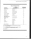 Methods
indices (USEPA, 1985d; Green, 1979; Hurlbert, 1971). Measures of biomass have
inherent problems in the collection of the data, e.g., loss or gain of weight due to
preservative medium, drying times, and evaporative weight loss. However, biomass,
used in conjunction with species composition and abundance data, may demonstrate
the relative effects of enrichment on benthic communities (Pearson and Rosenberg,
1978).
More complicated indices—e.g., species diversity, species richness, dominance,
evenness—have found varying degrees of acceptance. Diversity indices, measures of
the distribution of individuals among species, have the following limitations (Green,
1979):
• Often lack biological meaning;
• Are not robust empirical indicators of ecosystem "health";
• Do not incorporate information on form and function of resident species; and
• Are susceptible to biases associated with well-described taxa.
However, species diversity indices are a widely used measure of community structure
and provide a consistent level of data reduction for large-scale comparisons.
The dominance index is a measure of the degree to which one or a few species
dominate the community. The dominance index, herein defined as the minimum
number of species required to account for 75 percent of the total number of individuals,
has been useful in describing community structure (Swartz et al., 1985). It is easily
calculated, does not assume an underlying distribution of individuals among species,
and is statistically testable.
Several graphical analyses of these simple biological indices have been developed
although most require further study before their effectiveness is known. For example,
the use of Gray and Mirza's (1979) lognormal distribution of individuals per species and
Warwick's (1985) abundance-biomass comparison (ABC) methods, though useful for
some habitats, have been found to be unpredictable for other habitats and other locales
(USEPA, 1989e; Beukema, 1988). However, Pearson and Rosenberg's (1978)
species-abundance-biomass (SAB) model appears to be applicable to several forms of
environmental disturbance and may be used in conjunction with other analyses to
assess spatial and temporal impacts due to disturbance (Figure 4-2). The SAB model
provides a means to assess the condition of the habitat based on species numbers, total
abundance, and total biomass. Severely polluted areas are identified by the lack of
organisms, low species numbers, total abundance, and biomass. Highly polluted areas
are identified by a few, highly abundant populations of small-bodied, pollution-tolerant,
opportunistic species (e.g., Capitella capitata); total abundance is high, although
biomass and species numbers remain low. Less polluted areas (e.g., farther from a
116
image:
Methods
indices (USEPA, 1985d; Green, 1979; Hurlbert, 1971). Measures of biomass have
inherent problems in the collection of the data, e.g., loss or gain of weight due to
preservative medium, drying times, and evaporative weight loss. However, biomass,
used in conjunction with species composition and abundance data, may demonstrate
the relative effects of enrichment on benthic communities (Pearson and Rosenberg,
1978).
More complicated indices—e.g., species diversity, species richness, dominance,
evenness—have found varying degrees of acceptance. Diversity indices, measures of
the distribution of individuals among species, have the following limitations (Green,
1979):
• Often lack biological meaning;
• Are not robust empirical indicators of ecosystem "health";
• Do not incorporate information on form and function of resident species; and
• Are susceptible to biases associated with well-described taxa.
However, species diversity indices are a widely used measure of community structure
and provide a consistent level of data reduction for large-scale comparisons.
The dominance index is a measure of the degree to which one or a few species
dominate the community. The dominance index, herein defined as the minimum
number of species required to account for 75 percent of the total number of individuals,
has been useful in describing community structure (Swartz et al., 1985). It is easily
calculated, does not assume an underlying distribution of individuals among species,
and is statistically testable.
Several graphical analyses of these simple biological indices have been developed
although most require further study before their effectiveness is known. For example,
the use of Gray and Mirza's (1979) lognormal distribution of individuals per species and
Warwick's (1985) abundance-biomass comparison (ABC) methods, though useful for
some habitats, have been found to be unpredictable for other habitats and other locales
(USEPA, 1989e; Beukema, 1988). However, Pearson and Rosenberg's (1978)
species-abundance-biomass (SAB) model appears to be applicable to several forms of
environmental disturbance and may be used in conjunction with other analyses to
assess spatial and temporal impacts due to disturbance (Figure 4-2). The SAB model
provides a means to assess the condition of the habitat based on species numbers, total
abundance, and total biomass. Severely polluted areas are identified by the lack of
organisms, low species numbers, total abundance, and biomass. Highly polluted areas
are identified by a few, highly abundant populations of small-bodied, pollution-tolerant,
opportunistic species (e.g., Capitella capitata); total abundance is high, although
biomass and species numbers remain low. Less polluted areas (e.g., farther from a
116
image:
 Section 403 Procedural and Monitoring Guidance
B
Increasing organic input
PO = peak of opportunists
E = ecotone point
TR = transition zone
S = species numbers
B = total biomass
A = total abundance
Figure 4-2. Generalized SAB Diagram of Changes Along a Gradient of Organic
Enrichment (from Pearson and Rosenberg, 1978)
point source, or over time following the cessation of organic input) may be identified by
high species numbers and biomass, as more competitive, larger-bodied species are
able to tolerate sediment conditions. More pristine areas are characterized by a number
of small populations of competitively dominant species; species numbers remain
elevated, although biomass and total abundance are low. This approach, however,
requires the comparison of two or more sites along the pollution gradient.
For hard-bottom communities, some of the methods used successfully for detection of
pollutant impacts in soft-bottom communities (Warwick, 1986) appear to have little direct
application (Brown, 1988). For example, the sensitivity of diversity indices to describe
change in coral communities may be less than that of other parameters such as coral
cover, colony size, and abundance, suggesting that each parameter requires careful
analysis based on the previous environmental history of the site, the nature of the
impact, and the community structure of the reef. Grigg and Dollar (1990) have proposed
a stress index that measures net mortality of the organisms over time, partitioning the
mortality due to natural causes (N) and that due to man-made influence (I), thus allowing
these contributions to be compared. In terms of survival then:
117
image:
Section 403 Procedural and Monitoring Guidance
B
Increasing organic input
PO = peak of opportunists
E = ecotone point
TR = transition zone
S = species numbers
B = total biomass
A = total abundance
Figure 4-2. Generalized SAB Diagram of Changes Along a Gradient of Organic
Enrichment (from Pearson and Rosenberg, 1978)
point source, or over time following the cessation of organic input) may be identified by
high species numbers and biomass, as more competitive, larger-bodied species are
able to tolerate sediment conditions. More pristine areas are characterized by a number
of small populations of competitively dominant species; species numbers remain
elevated, although biomass and total abundance are low. This approach, however,
requires the comparison of two or more sites along the pollution gradient.
For hard-bottom communities, some of the methods used successfully for detection of
pollutant impacts in soft-bottom communities (Warwick, 1986) appear to have little direct
application (Brown, 1988). For example, the sensitivity of diversity indices to describe
change in coral communities may be less than that of other parameters such as coral
cover, colony size, and abundance, suggesting that each parameter requires careful
analysis based on the previous environmental history of the site, the nature of the
impact, and the community structure of the reef. Grigg and Dollar (1990) have proposed
a stress index that measures net mortality of the organisms over time, partitioning the
mortality due to natural causes (N) and that due to man-made influence (I), thus allowing
these contributions to be compared. In terms of survival then:
117
image:
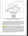 Methods
Stress Index = 1.0-(N + I),
where N +1 varies from 1 (total destruction) to 0 (zero mortality).
Although there are problems in applying this index in the field, development of a
quantitative index of stress would assist in the assessment of natural versus
anthropogenic contributions in hard-bottom benthic communities (Brown, 1988).
Indicator Species
Examination of abundances of individual indicator species are generally informative and
may reduce the cost of the analysis. The absence of pollution-sensitive species and the
enhancement of opportunistic and pollution-tolerant species may assist in defining the
spatial and temporal extent and magnitude of impacts. However, indicator variables
must possess the following characteristics (Green, 1979):
• Must provide a sufficiently precise and accurate appraisal of:
- species of concern,
- anthropogenic disturbances to benthic communities, and
- presence/absence or magnitude of anthropogenic perturbation to the
ecosystem.
• Must provide a cost-effective and statistically reliable alternative to monitoring
all critical benthic community measures of habitat perturbation.
• Must be appropriate for the spatial and temporal scale demanded by the
study objectives.
Pearson and Rosenberg (1978) demonstrated that along a gradient of organic
enrichment, a predictable community of benthic infauna could be observed (Figure 4-3).
Communities consist of opportunistic, tolerant species in areas of severe pollution,
giving way to less tolerant and more competitively dominant species further from
severely polluted areas (Figure 4-3). This model of indicator species composition and
distribution has been found to be useful in assessing both natural and anthropogenic
disturbances.
Several indices, derived from the distributions of pollution-sensitive species and
opportunistic disturbance-tolerant species, have been developed to evaluate impacts to
infaunal benthic community structures: copepod/nematode ratio (Raffaelli and Mason,
1981), infaunal trophic index (Word, 1978), and organism-sediment index (Rhoads and
Germane, 1986). The infaunal index, which was initially developed for the Southern
California Bight, uses the abundances of four functional groupings to describe
community structure. Low values of the infaunal index indicate communities dominated
118
image:
Methods
Stress Index = 1.0-(N + I),
where N +1 varies from 1 (total destruction) to 0 (zero mortality).
Although there are problems in applying this index in the field, development of a
quantitative index of stress would assist in the assessment of natural versus
anthropogenic contributions in hard-bottom benthic communities (Brown, 1988).
Indicator Species
Examination of abundances of individual indicator species are generally informative and
may reduce the cost of the analysis. The absence of pollution-sensitive species and the
enhancement of opportunistic and pollution-tolerant species may assist in defining the
spatial and temporal extent and magnitude of impacts. However, indicator variables
must possess the following characteristics (Green, 1979):
• Must provide a sufficiently precise and accurate appraisal of:
- species of concern,
- anthropogenic disturbances to benthic communities, and
- presence/absence or magnitude of anthropogenic perturbation to the
ecosystem.
• Must provide a cost-effective and statistically reliable alternative to monitoring
all critical benthic community measures of habitat perturbation.
• Must be appropriate for the spatial and temporal scale demanded by the
study objectives.
Pearson and Rosenberg (1978) demonstrated that along a gradient of organic
enrichment, a predictable community of benthic infauna could be observed (Figure 4-3).
Communities consist of opportunistic, tolerant species in areas of severe pollution,
giving way to less tolerant and more competitively dominant species further from
severely polluted areas (Figure 4-3). This model of indicator species composition and
distribution has been found to be useful in assessing both natural and anthropogenic
disturbances.
Several indices, derived from the distributions of pollution-sensitive species and
opportunistic disturbance-tolerant species, have been developed to evaluate impacts to
infaunal benthic community structures: copepod/nematode ratio (Raffaelli and Mason,
1981), infaunal trophic index (Word, 1978), and organism-sediment index (Rhoads and
Germane, 1986). The infaunal index, which was initially developed for the Southern
California Bight, uses the abundances of four functional groupings to describe
community structure. Low values of the infaunal index indicate communities dominated
118
image:
 Section 403 Procedural and Monitoring Quittance
Figure 4-3. Diagram of Changes in Fauna and Sediment Structure Along a Gradient of
Organic Enrichment (from Pearson and Rosenberg, 1978)
by deposit-feeding organisms that are considered to be more impacted than
communities dominated by suspension feeders (high infaunal index values)(Word,
1978).
Polluted or disturbed conditions may be indicated by:
• High rates of the nematode/copepod ratio;
• Low values (A) of the infaunal index; and
• Low values (7) of the organism-sediment index.
However, further studies of the response patterns of infaunal species subjected to
anthropogenic perturbations are required in order to select appropriate indicators of
benthic community impact. Again for hard-bottom communities, the use of epifaunal
indicator species and other indices requires further research (Brown, 1988).
It is recommended that multiple pollution-tolerant and pollution-sensitive indicator
species be selected by clearly defined criteria. Multiple indicator species often provide a
more complete representation of environmental conditions.
119
image:
Section 403 Procedural and Monitoring Quittance
Figure 4-3. Diagram of Changes in Fauna and Sediment Structure Along a Gradient of
Organic Enrichment (from Pearson and Rosenberg, 1978)
by deposit-feeding organisms that are considered to be more impacted than
communities dominated by suspension feeders (high infaunal index values)(Word,
1978).
Polluted or disturbed conditions may be indicated by:
• High rates of the nematode/copepod ratio;
• Low values (A) of the infaunal index; and
• Low values (7) of the organism-sediment index.
However, further studies of the response patterns of infaunal species subjected to
anthropogenic perturbations are required in order to select appropriate indicators of
benthic community impact. Again for hard-bottom communities, the use of epifaunal
indicator species and other indices requires further research (Brown, 1988).
It is recommended that multiple pollution-tolerant and pollution-sensitive indicator
species be selected by clearly defined criteria. Multiple indicator species often provide a
more complete representation of environmental conditions.
119
image:
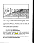 Methods
Multivariate Analyses
Numerical classification encompasses a wide variety of techniques that have been used in
the analysis of benthic data to distinguish groups of entities (e.g., sample locations)
according to similarity of attributes (e.g., species). These techniques differ from most
multivariate methods in that no assumptions are made concerning the underlying
distributions of the variables. Detailed descriptions of numerical classification analysis can
be found in Pielou (1984), Romesburg (1984), Clifford and Stephenson (1975), Boesch
(1977), Sneath and Sokal (1973), and Anderberg (1973). Boesch (1977) is particularly
valuable as an introduction and guide to the use of numerical classification analysis in
marine environmental studies. Guidance on the interpretation of classification results is
provided in an EPA Technical Support Document (USEPA, 1988d).
Ordination analyses have also been used to reduce the dimensionality of the data set while
maintaining the relationship among similar and dissimilar entities. At present, no single
ordination technique has been shown to be clearly superior for the analysis of biological data
(USEPA, 1985d).
Multivariate analyses are effective heuristic tools. They generate visual representations
that often indicate where further analyses ought to be conducted.
Analytical Approach Recommendations
Some of the most informative measures of community structure are the simplest (Table
4-20):
• Number of individuals,
• Number of species,
• Dominance,
• Infaunal index,
• Abundances of pollution-sensitive species, and
• Abundance of opportunistic and pollution-tolerant species.
These indices have proved to be useful over various habitats and regions in assessing
changes to benthic community structures (USEPA, 1985d). Values of these indices may
be determined from the list of species abundances generated during the taxonomic
identifications of collected specimens. Furthermore, the values of these six variables may
be easily tested statistically using parametric or nonparametric techniques. It is
recommended that no single index or analytical method be used to assess impacts;
instead, the assessment of impacts should incorporate information that each variable
and method contributes concerning benthic community structure.
120
image:
Methods
Multivariate Analyses
Numerical classification encompasses a wide variety of techniques that have been used in
the analysis of benthic data to distinguish groups of entities (e.g., sample locations)
according to similarity of attributes (e.g., species). These techniques differ from most
multivariate methods in that no assumptions are made concerning the underlying
distributions of the variables. Detailed descriptions of numerical classification analysis can
be found in Pielou (1984), Romesburg (1984), Clifford and Stephenson (1975), Boesch
(1977), Sneath and Sokal (1973), and Anderberg (1973). Boesch (1977) is particularly
valuable as an introduction and guide to the use of numerical classification analysis in
marine environmental studies. Guidance on the interpretation of classification results is
provided in an EPA Technical Support Document (USEPA, 1988d).
Ordination analyses have also been used to reduce the dimensionality of the data set while
maintaining the relationship among similar and dissimilar entities. At present, no single
ordination technique has been shown to be clearly superior for the analysis of biological data
(USEPA, 1985d).
Multivariate analyses are effective heuristic tools. They generate visual representations
that often indicate where further analyses ought to be conducted.
Analytical Approach Recommendations
Some of the most informative measures of community structure are the simplest (Table
4-20):
• Number of individuals,
• Number of species,
• Dominance,
• Infaunal index,
• Abundances of pollution-sensitive species, and
• Abundance of opportunistic and pollution-tolerant species.
These indices have proved to be useful over various habitats and regions in assessing
changes to benthic community structures (USEPA, 1985d). Values of these indices may
be determined from the list of species abundances generated during the taxonomic
identifications of collected specimens. Furthermore, the values of these six variables may
be easily tested statistically using parametric or nonparametric techniques. It is
recommended that no single index or analytical method be used to assess impacts;
instead, the assessment of impacts should incorporate information that each variable
and method contributes concerning benthic community structure.
120
image:
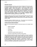 Section 403 Procedural and Monitoring Guidance
Selection of reference sites is key to the evaluation of environmental impact
assessment. Results of analyses using reference measures provide the means of
comparison by which anthropogenic impacts are detected. It is essential that selected
reference sites exhibit at least similar:
• Sediment characteristics (i.e., grain size or substratum type),
• Water depths,
• Flow characteristics,
• Salinity,
• Dissolved oxygen, and
• Temperature
compared to monitoring program sampling sites. Several reference sites may be
required to meet these criteria.
4.5.4 QA/QC Considerations
Sample Collection
Surveying and sampling equipment should be inspected for wear and tear to avoid loss
of data or sample leakage and loss upon ascent. It is recommended that backup survey
and sampling equipment be available on board the vessel in case the primary
equipment breaks down or is lost during the cruise.
The following infauna sample acceptability criteria should be satisfied (USEPA,
1986-1991):
• Sediment is not extruded from the upper face of the sampler such that
organisms may have been lost.
• Overlying water is present, indicating minimal leakage.
• The sediment surface is relatively flat, indicating minimal disturbance or
winnowing (Figure 4-4).
• The entire surface of the sample is included in the sampler.
• The desired penetration depth is achieved.
If the sample does not meet all the criteria, it should be rejected.
121
image:
Section 403 Procedural and Monitoring Guidance
Selection of reference sites is key to the evaluation of environmental impact
assessment. Results of analyses using reference measures provide the means of
comparison by which anthropogenic impacts are detected. It is essential that selected
reference sites exhibit at least similar:
• Sediment characteristics (i.e., grain size or substratum type),
• Water depths,
• Flow characteristics,
• Salinity,
• Dissolved oxygen, and
• Temperature
compared to monitoring program sampling sites. Several reference sites may be
required to meet these criteria.
4.5.4 QA/QC Considerations
Sample Collection
Surveying and sampling equipment should be inspected for wear and tear to avoid loss
of data or sample leakage and loss upon ascent. It is recommended that backup survey
and sampling equipment be available on board the vessel in case the primary
equipment breaks down or is lost during the cruise.
The following infauna sample acceptability criteria should be satisfied (USEPA,
1986-1991):
• Sediment is not extruded from the upper face of the sampler such that
organisms may have been lost.
• Overlying water is present, indicating minimal leakage.
• The sediment surface is relatively flat, indicating minimal disturbance or
winnowing (Figure 4-4).
• The entire surface of the sample is included in the sampler.
• The desired penetration depth is achieved.
If the sample does not meet all the criteria, it should be rejected.
121
image:
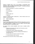 Methods
Acceptable if Minimum
Penetration Requirement Met
and Overlying Water is Present
Unacceptable-
(Canted with Partial Sample)
Unacceptable
(Washed, Rock Caught in Jaws)
Unacceptable
(Washed)
Figure 4-4. Examples of Acceptable and Unacceptable Samples (USEPA, 1987c)
Appropriate QA/QC protocols for assessing the validity of hard-bottom surveys (e.g.,
multiple transects, resurveying one or more transects or quadrats by different divers)
should also be followed.
Taxonomic Identification
A key QA/QC issue is taxonomic standardization. Consistent taxonomic identifications
are achieved through interaction among taxonomists working on each major group.
Participation of the laboratory staff in regional taxonomic standardization programs is
recommended to ensure regional consistency and accuracy of identifications.
Five percent of all samples identified by one taxonomist should be reidentified by
another taxonomist who is also qualified to identify organisms in that major group.
It is advisable that at least three individuals of each taxon should be sent for verification
to recognized experts. These verified specimens should then be placed in a permanent
reference collection. All specimens in the reference collection should be stored in
labeled vials that are segregated by species and sample. Reference specimens should
be archived alphabetically within major taxonomic groups.
122
image:
Methods
Acceptable if Minimum
Penetration Requirement Met
and Overlying Water is Present
Unacceptable-
(Canted with Partial Sample)
Unacceptable
(Washed, Rock Caught in Jaws)
Unacceptable
(Washed)
Figure 4-4. Examples of Acceptable and Unacceptable Samples (USEPA, 1987c)
Appropriate QA/QC protocols for assessing the validity of hard-bottom surveys (e.g.,
multiple transects, resurveying one or more transects or quadrats by different divers)
should also be followed.
Taxonomic Identification
A key QA/QC issue is taxonomic standardization. Consistent taxonomic identifications
are achieved through interaction among taxonomists working on each major group.
Participation of the laboratory staff in regional taxonomic standardization programs is
recommended to ensure regional consistency and accuracy of identifications.
Five percent of all samples identified by one taxonomist should be reidentified by
another taxonomist who is also qualified to identify organisms in that major group.
It is advisable that at least three individuals of each taxon should be sent for verification
to recognized experts. These verified specimens should then be placed in a permanent
reference collection. All specimens in the reference collection should be stored in
labeled vials that are segregated by species and sample. Reference specimens should
be archived alphabetically within major taxonomic groups.
122
image:
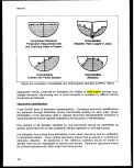 Section 403 Procedural and Monitoring Guidance
It is also recommended that at least 20 percent of each sample be re-sorted for QA/QC
purposes. Re-sorting is the examination of a sample or subsample that has been sorted
once and is considered free of organisms. Re-sorting should be done by someone other
than the one who sorted the original sample. If a sample is found that does not meet the
recommended 95 percent removal criterion, the entire sample should be re-sorted. For
epifaunal surveys, a portion of the photographed quadrats should be reanalyzed for
comparisons.
4.5.5 Statistical Design Considerations
Consideration of statistical strategies will mitigate the high costs of collecting and
processing samples.
Temporal Stratification of the Data
The time of the year should be controlled or stratified in the design; the use of annual
averages is seldom a good practice. Temporal stratification of the data should not be
attempted until sufficient knowledge of long-term natural cycles is attained. Initially,
simple regression analyses may be conducted on seasonally stratified data to identify
monotonic temporal trends. Further examinations of whether conditions are improving
or degrading over time may be performed using various statistical time series analyses.
Statistical Power
Selection of the number of replicates is an important component of program design.
The inherent patchiness of benthic communities requires collection of sufficient replicate
samples to ensure an accurate description of the benthos. However, increases in
replication increase sample processing costs. Power analyses assist in the allocation of
sampling resources (stations, replication, and frequency) with regard to program
finances and design.
Power analyses may be applied to determine the appropriate number of sample
replicates required to detect a specified difference (USEPA, 1987d). The number of
replications required to detect a specified minimum difference is a function of the
statistical power and the variance in the data. Power analyses require a priori
knowledge of the variability in the data. A best guess or, preferably, variation observed
in historical data is often used initially in the design of the monitoring program.
To improve the power of a statistical test, while keeping the significance level constant,
the sample size (area sampled, number of replicates of grabs, quadrats, or transects)
should be increased. Because of constraints in cost and time, however, this option may
not be available. Power analysis has shown that for a fixed level of sampling effort, a
monitoring program's power is generally increased by collecting more replicates at fewer
locations. Sampling should be conducted in a radiating pattern from the zone of initial
discharge out to the distance where there will be no effects.
123
image:
Section 403 Procedural and Monitoring Guidance
It is also recommended that at least 20 percent of each sample be re-sorted for QA/QC
purposes. Re-sorting is the examination of a sample or subsample that has been sorted
once and is considered free of organisms. Re-sorting should be done by someone other
than the one who sorted the original sample. If a sample is found that does not meet the
recommended 95 percent removal criterion, the entire sample should be re-sorted. For
epifaunal surveys, a portion of the photographed quadrats should be reanalyzed for
comparisons.
4.5.5 Statistical Design Considerations
Consideration of statistical strategies will mitigate the high costs of collecting and
processing samples.
Temporal Stratification of the Data
The time of the year should be controlled or stratified in the design; the use of annual
averages is seldom a good practice. Temporal stratification of the data should not be
attempted until sufficient knowledge of long-term natural cycles is attained. Initially,
simple regression analyses may be conducted on seasonally stratified data to identify
monotonic temporal trends. Further examinations of whether conditions are improving
or degrading over time may be performed using various statistical time series analyses.
Statistical Power
Selection of the number of replicates is an important component of program design.
The inherent patchiness of benthic communities requires collection of sufficient replicate
samples to ensure an accurate description of the benthos. However, increases in
replication increase sample processing costs. Power analyses assist in the allocation of
sampling resources (stations, replication, and frequency) with regard to program
finances and design.
Power analyses may be applied to determine the appropriate number of sample
replicates required to detect a specified difference (USEPA, 1987d). The number of
replications required to detect a specified minimum difference is a function of the
statistical power and the variance in the data. Power analyses require a priori
knowledge of the variability in the data. A best guess or, preferably, variation observed
in historical data is often used initially in the design of the monitoring program.
To improve the power of a statistical test, while keeping the significance level constant,
the sample size (area sampled, number of replicates of grabs, quadrats, or transects)
should be increased. Because of constraints in cost and time, however, this option may
not be available. Power analysis has shown that for a fixed level of sampling effort, a
monitoring program's power is generally increased by collecting more replicates at fewer
locations. Sampling should be conducted in a radiating pattern from the zone of initial
discharge out to the distance where there will be no effects.
123
image:
 Methods
4.5.6
Use of Data
Monitoring of benthic community structure provides in situ measures of the benthic
habitat and is a powerful tool in the evaluation of spatial and temporal effects of
anthropogenic and natural disturbance. The presence or absence of certain organisms
is useful in indicating the previous condition of the environment (Bilyard, 1987; Tomascik
and Saunder, 1987). Monitoring of benthic infaunal communities also provides data
required in the design and validation of benthic community dynamics models (Pearson
and Rosenberg, 1978; Brown, 1988) and the selection of biological indicators (Word,
1978).
In addition, monitoring of benthic communities directly provides accurate information
essential in assessing the effectiveness of discharge reductions (Bilyard, 1987). For
example, benthic infauna monitoring provided information used to assess the
effectiveness of pollution abatement plans in the recovery of Southern California waters
(Reish, 1986; SCCWRP, 1988). These studies indicate that analyses of benthic
communities may be effectively used to monitor the long-term health of the receiving
environment (Reish, 1986).
i
Currently, benthic communities have not proved useful for identifying specific chemicals
or classes of chemicals present in the environment. Further information concerning
specific responses to specific contaminants is required before infaunal community
structure becomes useful in identifying specific contaminants (USEPA, 1989e). In
addition, caution is recommended in the use of benthic community structure to predict
specific effects on potential predators. Information on trophic relationships, competition,
and predation is often not available. The capability to predict the effects of altered prey
communities on predators may improve with research on these topics. Factors such as
prey quality, distribution of prey, and interactions among species will be important
components of this research.
However, benthic invertebrates do serve as effective indicators of environmental
condition, delineating the magnitude, spatial extent, and temporal trends of
anthropogenic and natural perturbations to the ecosystem (Reish, 1986; Bilyard, 1987).
Monitoring of benthic infauna and epifauna will provide relevant accurate data
fundamental to achieving the objectives of most monitoring programs.
4.5.7 Summary and Recommendations
Rationale
The objective is to detect and describe spatial and temporal changes in the
structure and function of benthic communities.
124
image:
Methods
4.5.6
Use of Data
Monitoring of benthic community structure provides in situ measures of the benthic
habitat and is a powerful tool in the evaluation of spatial and temporal effects of
anthropogenic and natural disturbance. The presence or absence of certain organisms
is useful in indicating the previous condition of the environment (Bilyard, 1987; Tomascik
and Saunder, 1987). Monitoring of benthic infaunal communities also provides data
required in the design and validation of benthic community dynamics models (Pearson
and Rosenberg, 1978; Brown, 1988) and the selection of biological indicators (Word,
1978).
In addition, monitoring of benthic communities directly provides accurate information
essential in assessing the effectiveness of discharge reductions (Bilyard, 1987). For
example, benthic infauna monitoring provided information used to assess the
effectiveness of pollution abatement plans in the recovery of Southern California waters
(Reish, 1986; SCCWRP, 1988). These studies indicate that analyses of benthic
communities may be effectively used to monitor the long-term health of the receiving
environment (Reish, 1986).
i
Currently, benthic communities have not proved useful for identifying specific chemicals
or classes of chemicals present in the environment. Further information concerning
specific responses to specific contaminants is required before infaunal community
structure becomes useful in identifying specific contaminants (USEPA, 1989e). In
addition, caution is recommended in the use of benthic community structure to predict
specific effects on potential predators. Information on trophic relationships, competition,
and predation is often not available. The capability to predict the effects of altered prey
communities on predators may improve with research on these topics. Factors such as
prey quality, distribution of prey, and interactions among species will be important
components of this research.
However, benthic invertebrates do serve as effective indicators of environmental
condition, delineating the magnitude, spatial extent, and temporal trends of
anthropogenic and natural perturbations to the ecosystem (Reish, 1986; Bilyard, 1987).
Monitoring of benthic infauna and epifauna will provide relevant accurate data
fundamental to achieving the objectives of most monitoring programs.
4.5.7 Summary and Recommendations
Rationale
The objective is to detect and describe spatial and temporal changes in the
structure and function of benthic communities.
124
image:
 Section 403 Procedural and Monitoring Guidance
• Benthic monitoring provides in situ measures of habitat quality and is a
powerful tool in assessing environmental impact.
Monitoring Design Considerations
• It is recommended that consistent types of surveying and sampling gear, data
collection and sample sorting protocols, level of taxonomy, and location and
timing of sample collection be implemented to allow for comparisons between
studies.
• To reduce the variation due to seasonal differences, sampling should be
conducted during the same season—preferably the same month—each year.
• Voucher specimens should be collected for in situ epifaunal surveys.
• For epifaunal surveys, data are collected on species and organism coverage
of the substratum by diver, ROV, or submarine from specified transects or
quadrats.
• For infaunal sampling, collection of undisturbed sediment requires that the
sampler:
- create a minimal bow wake when descending;
- form a leakproof seal when the sediment sample is taken;
- prevent winnowing and excessive sample disturbance when ascending; and
- allow easy access to the sample surface in order that undisturbed
subsamples may be taken.
• Penetration well below the desired sampling depth is preferred to prevent
soft-bottom disturbance as the device closes.
• Grab samplers and box corers are recognized as the tools of choice for
maximum accuracy and precision when sampling soft-bottom habitats.
• Sorting through a standard sieve mesh size (i.e., 0.5 mm) is recommended.
Further sorting through other mesh sizes may be conducted in addition to
sorting through this standard mesh size.
• Relaxants facilitate identification and morphometric measurements; however,
standard procedures must be implemented to ensure valid comparisons
among studies.
• Vital stains may facilitate sorting; however, a proper QA program should
ensure that sorting efficiency is maintained.
• Identifications to higher taxonomic levels may be sufficient to meet program
objectives; however, it is recommended that all samples be archived if
comparisons to lower taxonomic levels will be required at a later date.
125
image:
Section 403 Procedural and Monitoring Guidance
• Benthic monitoring provides in situ measures of habitat quality and is a
powerful tool in assessing environmental impact.
Monitoring Design Considerations
• It is recommended that consistent types of surveying and sampling gear, data
collection and sample sorting protocols, level of taxonomy, and location and
timing of sample collection be implemented to allow for comparisons between
studies.
• To reduce the variation due to seasonal differences, sampling should be
conducted during the same season—preferably the same month—each year.
• Voucher specimens should be collected for in situ epifaunal surveys.
• For epifaunal surveys, data are collected on species and organism coverage
of the substratum by diver, ROV, or submarine from specified transects or
quadrats.
• For infaunal sampling, collection of undisturbed sediment requires that the
sampler:
- create a minimal bow wake when descending;
- form a leakproof seal when the sediment sample is taken;
- prevent winnowing and excessive sample disturbance when ascending; and
- allow easy access to the sample surface in order that undisturbed
subsamples may be taken.
• Penetration well below the desired sampling depth is preferred to prevent
soft-bottom disturbance as the device closes.
• Grab samplers and box corers are recognized as the tools of choice for
maximum accuracy and precision when sampling soft-bottom habitats.
• Sorting through a standard sieve mesh size (i.e., 0.5 mm) is recommended.
Further sorting through other mesh sizes may be conducted in addition to
sorting through this standard mesh size.
• Relaxants facilitate identification and morphometric measurements; however,
standard procedures must be implemented to ensure valid comparisons
among studies.
• Vital stains may facilitate sorting; however, a proper QA program should
ensure that sorting efficiency is maintained.
• Identifications to higher taxonomic levels may be sufficient to meet program
objectives; however, it is recommended that all samples be archived if
comparisons to lower taxonomic levels will be required at a later date.
125
image:
 Methods
Analytical Methods Considerations
• It is recommended that simple measures of community structure be used to
assess the condition of the benthos: number of individuals, number of
species, dominance, infaunal index, abundance of pollution-sensitive
species, abundance of pollution-tolerant species, and percent cover for
hard-bottom indicator groups.
• Selected biological indices should retain biological meaning, be robust
indicators of ecosystem "health," and incorporate species form and function.
• Indicator species should possess the following characteristics:
- sensitive to benthic perturbations of concern;
- cost-effective and statistically reliable alternative to measuring all species
in a monitoring program;
- statistically reliable indicative measures of habitat perturbations; and
- appropriate for the spatial and temporal scale demanded by the study
objectives.
• Selection of reference sites is key to the evaluation of environmental impact
due to anthropogenic impacts; several reference sites may be required.
QA/QC Considerations
• Taxonomic standardization is essential to the analysis of community
structure. Recommended protocols include consistent interactions among
taxonomists, reidentification of selected samples, use of a reference
collection, and re-sorting and analysis of selected samples or subsamples.
Statistical Design Considerations
• Power analyses may be applied to determine the appropriate number of
sample replicates required to detect a specified difference, thereby optimizing
the high costs of collecting and processing samples.
Use of Data
• Data provide essential information in order to assess impacts due to
anthropogenic perturbation, monitor recovery of the receiving environment,
and validate community and population models.
126
image:
Methods
Analytical Methods Considerations
• It is recommended that simple measures of community structure be used to
assess the condition of the benthos: number of individuals, number of
species, dominance, infaunal index, abundance of pollution-sensitive
species, abundance of pollution-tolerant species, and percent cover for
hard-bottom indicator groups.
• Selected biological indices should retain biological meaning, be robust
indicators of ecosystem "health," and incorporate species form and function.
• Indicator species should possess the following characteristics:
- sensitive to benthic perturbations of concern;
- cost-effective and statistically reliable alternative to measuring all species
in a monitoring program;
- statistically reliable indicative measures of habitat perturbations; and
- appropriate for the spatial and temporal scale demanded by the study
objectives.
• Selection of reference sites is key to the evaluation of environmental impact
due to anthropogenic impacts; several reference sites may be required.
QA/QC Considerations
• Taxonomic standardization is essential to the analysis of community
structure. Recommended protocols include consistent interactions among
taxonomists, reidentification of selected samples, use of a reference
collection, and re-sorting and analysis of selected samples or subsamples.
Statistical Design Considerations
• Power analyses may be applied to determine the appropriate number of
sample replicates required to detect a specified difference, thereby optimizing
the high costs of collecting and processing samples.
Use of Data
• Data provide essential information in order to assess impacts due to
anthropogenic perturbation, monitor recovery of the receiving environment,
and validate community and population models.
126
image:
 Section 403 Procedural and Monitoring Guidance
4.6
FISH AND SHELLFISH PATHOBIOLOGY
Pathobiological methods provide information concerning damage to organ systems of
fish and shellfish through an evaluation of their structure, activity, and function.
Anatomic pathology methods can give an indication of the nature of an altered state, for
example, by identifying the specific type of tumor present in an animal. Reproductive
developmental studies examine the reproductive capacity of animals and can provide
information to aid in estimating and predicting population abundance and recruitment.
Biochemical/enzymological studies seek to detect differences in enzymatic activity as a
measure of biological condition. Immunological methods can demonstrate altered
immune response, an indicator of changes in bodily defense mechanisms and increased
susceptibility to disease.
Pathobiological methods should be used in concert to investigate cause-and-effect
relationships as a result of contaminant exposure. Anatomic pathology can serve as a
vital link between observed effects on populations and communities in an estuary and
the changes in activity and function observed by other methods.
4.6.1
Rationale
Pathobiological methods can be used to examine adverse effects of pollutants on fish
and shellfish. The presence of toxics in water and sediments may not immediately
result in visible changes in these organisms. Biomarkers offer a more sensitive and
reliable assessment of exposure risks than ambient water or sediment quality
monitoring. Monitoring of pathobiological effects provides information necessary to
make determinations of the existence of adverse effects in animals (e.g., tumors),
population productivity and stability (affected by reproduction and disease states), and
the loss of organisms deemed valuable for ecological, aesthetic, recreational, scientific,
or economic reasons. Table 4-21 outlines some of the terms used to describe
pathobiological methods.
Although the value of these methods for establishing cause-and-effect links has been
established during laboratory toxicity studies, some questions remain regarding their ability
to establish such links for field-collected organisms that are exposed to a variety of natural
environmental stresses and combinations of contaminants (Hinton and Couch, 1984; Couch
and Harshbarger, 1985; Mix, 1986; Sindermann, 1990). However, properly conducted
multidisciplinary monitoring studies using these methods can provide regulatory agencies
with evidence of impaired health status in animals exposed to contaminants in estuarine
ecosystems. This information can then be used to direct laboratory confirmation of the
cause, if necessary (see, for example, Buckley etal., 1985; Gardner et al., 1991). Continued
monitoring with these methods can be used to detect changes in a population's health
during and following environmental intervention. Because changes at the organismal
level precede changes in population and community characteristics, pathobiological
studies can provide an early indication of the effectiveness of management actions.
127
image:
Section 403 Procedural and Monitoring Guidance
4.6
FISH AND SHELLFISH PATHOBIOLOGY
Pathobiological methods provide information concerning damage to organ systems of
fish and shellfish through an evaluation of their structure, activity, and function.
Anatomic pathology methods can give an indication of the nature of an altered state, for
example, by identifying the specific type of tumor present in an animal. Reproductive
developmental studies examine the reproductive capacity of animals and can provide
information to aid in estimating and predicting population abundance and recruitment.
Biochemical/enzymological studies seek to detect differences in enzymatic activity as a
measure of biological condition. Immunological methods can demonstrate altered
immune response, an indicator of changes in bodily defense mechanisms and increased
susceptibility to disease.
Pathobiological methods should be used in concert to investigate cause-and-effect
relationships as a result of contaminant exposure. Anatomic pathology can serve as a
vital link between observed effects on populations and communities in an estuary and
the changes in activity and function observed by other methods.
4.6.1
Rationale
Pathobiological methods can be used to examine adverse effects of pollutants on fish
and shellfish. The presence of toxics in water and sediments may not immediately
result in visible changes in these organisms. Biomarkers offer a more sensitive and
reliable assessment of exposure risks than ambient water or sediment quality
monitoring. Monitoring of pathobiological effects provides information necessary to
make determinations of the existence of adverse effects in animals (e.g., tumors),
population productivity and stability (affected by reproduction and disease states), and
the loss of organisms deemed valuable for ecological, aesthetic, recreational, scientific,
or economic reasons. Table 4-21 outlines some of the terms used to describe
pathobiological methods.
Although the value of these methods for establishing cause-and-effect links has been
established during laboratory toxicity studies, some questions remain regarding their ability
to establish such links for field-collected organisms that are exposed to a variety of natural
environmental stresses and combinations of contaminants (Hinton and Couch, 1984; Couch
and Harshbarger, 1985; Mix, 1986; Sindermann, 1990). However, properly conducted
multidisciplinary monitoring studies using these methods can provide regulatory agencies
with evidence of impaired health status in animals exposed to contaminants in estuarine
ecosystems. This information can then be used to direct laboratory confirmation of the
cause, if necessary (see, for example, Buckley etal., 1985; Gardner et al., 1991). Continued
monitoring with these methods can be used to detect changes in a population's health
during and following environmental intervention. Because changes at the organismal
level precede changes in population and community characteristics, pathobiological
studies can provide an early indication of the effectiveness of management actions.
127
image:
 Methods
biomarker
cytochrome P450
cytogenetics
genotoxic agents
hepatic
histopathology
hfstochemistry
immunoassay
immunology
inclusion bodies
macrophage
pathobiology
smooth endoplasmic
reticulum (SER)
Table 4-21. List of Pathobiological Terms
any biological method used to detect the exposure of organisms to hazardous
chemicals in the environment by measuring the response of the organisms to the
contaminant through comparative molecular, biochemical, physiological, or
anatomical observations of cellular dysfunction
a protein in the microsomes of liver cells that is important in catalyzing the
metabolism of steroid hormones and fatty acids and in the detoxification of a variety
of chemical substances
the study of cytology in relation to genetics, especially the study of chromosomal
behavior in mitosis and meiosis. Modern cytogenetics has led to the identification of
chromosomes as bearers of the genes and deoxyribonucleic acid (DMA) as the key
molecule of the gene
chemical and physical agents that can produce genetic alterations at subtoxic
concentrations and can result in altered heredity characteristics. Genotoxic agents
generally possess specified chemical or physical properties that facilitate their
interaction with nucleic acids
of, or relating to, the liver
pathologic histology; the science or study dealing with the cytologic and histologic
(microscopic) structure of abnormal or diseased cells, tissues, and organs in relation
to their function
the study of the chemistry of cells and tissues using light and electron microscopy,
special chemical tests, and special stains to determine the location of certain enzyme
systems or reaction products in the cell
measuring the protein and protein-bound molecules that are concerned with the
reaction of an antigen with its specific antibody, as in the detection of hormones or
other substances
the study of being protected from a disease; the study of the response of the body
and its tissues to a variety of antigens, including red cells, pollens, transplanted
tissues, and even the individual's own cells
bodies present in the nucleus or cytoplasm of certain cells in cases of infection by
filtrable viruses or as the result of degenerative diseases or exposure to chemicals
cells of the reticuloendothelial system having the ability to phagocytose particulate
substances and to store vital dyes and other colloidal substances
pathology, the study of disease, with emphasis more on the biological than the
medical aspects of the essential nature, causes, and development of abnormal
conditions, as well as the structural and functional changes that result from the
disease process
a connecting network of tubules that course through the cytoplasm of the cell and can
be viewed using the electron microscope; SER is essential to metabolic functions of
the cells
SOURCES: Stedman's Medical Dictionary, 1982; Taber"s Cyclopedic Medical Dictionary, 1985.
EL'
.<
mSA
•:ir
128
image:
Methods
biomarker
cytochrome P450
cytogenetics
genotoxic agents
hepatic
histopathology
hfstochemistry
immunoassay
immunology
inclusion bodies
macrophage
pathobiology
smooth endoplasmic
reticulum (SER)
Table 4-21. List of Pathobiological Terms
any biological method used to detect the exposure of organisms to hazardous
chemicals in the environment by measuring the response of the organisms to the
contaminant through comparative molecular, biochemical, physiological, or
anatomical observations of cellular dysfunction
a protein in the microsomes of liver cells that is important in catalyzing the
metabolism of steroid hormones and fatty acids and in the detoxification of a variety
of chemical substances
the study of cytology in relation to genetics, especially the study of chromosomal
behavior in mitosis and meiosis. Modern cytogenetics has led to the identification of
chromosomes as bearers of the genes and deoxyribonucleic acid (DMA) as the key
molecule of the gene
chemical and physical agents that can produce genetic alterations at subtoxic
concentrations and can result in altered heredity characteristics. Genotoxic agents
generally possess specified chemical or physical properties that facilitate their
interaction with nucleic acids
of, or relating to, the liver
pathologic histology; the science or study dealing with the cytologic and histologic
(microscopic) structure of abnormal or diseased cells, tissues, and organs in relation
to their function
the study of the chemistry of cells and tissues using light and electron microscopy,
special chemical tests, and special stains to determine the location of certain enzyme
systems or reaction products in the cell
measuring the protein and protein-bound molecules that are concerned with the
reaction of an antigen with its specific antibody, as in the detection of hormones or
other substances
the study of being protected from a disease; the study of the response of the body
and its tissues to a variety of antigens, including red cells, pollens, transplanted
tissues, and even the individual's own cells
bodies present in the nucleus or cytoplasm of certain cells in cases of infection by
filtrable viruses or as the result of degenerative diseases or exposure to chemicals
cells of the reticuloendothelial system having the ability to phagocytose particulate
substances and to store vital dyes and other colloidal substances
pathology, the study of disease, with emphasis more on the biological than the
medical aspects of the essential nature, causes, and development of abnormal
conditions, as well as the structural and functional changes that result from the
disease process
a connecting network of tubules that course through the cytoplasm of the cell and can
be viewed using the electron microscope; SER is essential to metabolic functions of
the cells
SOURCES: Stedman's Medical Dictionary, 1982; Taber"s Cyclopedic Medical Dictionary, 1985.
EL'
.<
mSA
•:ir
128
image:
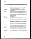 Section 403 Procedural and Monitoring Guidance
4.6.2 Monitoring Design Considerations
A field survey to collect target organisms and tissue samples may be required for
pathobiological monitoring (Hargis et al., 1984; U.S. EPA, 1987b). In certain instances,
a large sample size may be needed to establish statistical significance because of
normal variation from animal to animal, species and generic differences, and migratory
habits of fish. For these reasons, and the labor-intensive nature of pathobiological
methods, the availability and allocation of funds, time, equipment, and trained personnel
must be considered when planning to include pathobiological methods in monitoring
programs.
Selection of Target (Indicator) Species
A key component of any pathobiological monitoring program is the selection of target
species. The fundamental criterion is the ability to use the selected species to make
comparisons between sampling locations and sampling periods. It is recommended that
the target species possess the following characteristics:
• Abundant enough, temporally and spatially, to allow for adequate sampling;
• Large enough to provide adequate amounts of tissue for analysis;
• Sedentary (nonmigratory) in nature to ensure that pathobiological
abnormalities are representative of the study area; and
• Easily collected.
It is also recommended that an existing database documenting exposures and
sensitivities of the target organism specific to contaminants of concern is available.
Fish provide sufficient tissue for analyses and may indicate potential threats to human
populations. However, fish are motile and pathobiological abnormalities detected may
not be representative of the study area (see Vogelbein et al., 1990).
Bivalve molluscs, either attached to the substratum or burrowing in sediments, have
been sampled extensively to examine the condition of these commercially important
estuarine species (e.g., Mussel Watch, National Status and Trends program). The most
common target species have been oysters (Crassostrea virginica) and mussels (Mytilus
spp.), although pathobiological and bioassay studies have also been performed on other
species, such as crabs and penaeid shrimp.
Secondary considerations, based on economic importance and status as a bioassay
organism, may be applied to further winnow the list of candidate target species to a
practical number of species to be analyzed.
129
image:
Section 403 Procedural and Monitoring Guidance
4.6.2 Monitoring Design Considerations
A field survey to collect target organisms and tissue samples may be required for
pathobiological monitoring (Hargis et al., 1984; U.S. EPA, 1987b). In certain instances,
a large sample size may be needed to establish statistical significance because of
normal variation from animal to animal, species and generic differences, and migratory
habits of fish. For these reasons, and the labor-intensive nature of pathobiological
methods, the availability and allocation of funds, time, equipment, and trained personnel
must be considered when planning to include pathobiological methods in monitoring
programs.
Selection of Target (Indicator) Species
A key component of any pathobiological monitoring program is the selection of target
species. The fundamental criterion is the ability to use the selected species to make
comparisons between sampling locations and sampling periods. It is recommended that
the target species possess the following characteristics:
• Abundant enough, temporally and spatially, to allow for adequate sampling;
• Large enough to provide adequate amounts of tissue for analysis;
• Sedentary (nonmigratory) in nature to ensure that pathobiological
abnormalities are representative of the study area; and
• Easily collected.
It is also recommended that an existing database documenting exposures and
sensitivities of the target organism specific to contaminants of concern is available.
Fish provide sufficient tissue for analyses and may indicate potential threats to human
populations. However, fish are motile and pathobiological abnormalities detected may
not be representative of the study area (see Vogelbein et al., 1990).
Bivalve molluscs, either attached to the substratum or burrowing in sediments, have
been sampled extensively to examine the condition of these commercially important
estuarine species (e.g., Mussel Watch, National Status and Trends program). The most
common target species have been oysters (Crassostrea virginica) and mussels (Mytilus
spp.), although pathobiological and bioassay studies have also been performed on other
species, such as crabs and penaeid shrimp.
Secondary considerations, based on economic importance and status as a bioassay
organism, may be applied to further winnow the list of candidate target species to a
practical number of species to be analyzed.
129
image:
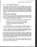 Methods
Sampling Location
Appropriate locations of sampling stations depend on the objectives of the study. For
example, to evaluate whether there is a statistically significant increase in lesions,
stations should be located to collect specimens from contaminated and uncontaminated
(background or control) areas for statistical comparison. It is also important to
demonstrate a dose-response relationship between the pollutant concentration and
incidence of tumors or other lesions by locating sample stations along a contamination
gradient (i.e., from highly contaminated to moderately contaminated to uncontaminated).
It is recommended that stations be located in areas where the geographic area of
contamination is large enough that sampled fish could reasonably be expected to have
spent a considerable amount of time within the influence of the pollutant (U.S. EPA,
1987b). Nielsen and Johnson (1984) and Cailliet et al. (1986) may be consulted for
further fish sampling methodologies. Information on sampling bivalves and other
invertebrates is contained in Couch (1978), Yevich and Barszcz (1983), Turgeon et al.
(1991), and other sources.
4.6.3 Analytical Methods Considerations
Anatomic Pathology Methods
Anatomic pathology methods examine tissues with the naked eye (gross anatomic
pathology), the aid of a light microscope (LM methods), or the electron microscope (EM
methods). Gross anatomic methods are concerned with obvious adverse changes in
tissue that can be observed in the field (Hunn, 1988; Hargis et al., 1984). The
advantage of gross methods is that large numbers of specimens can be examined
rapidly. However, the methods are generally nonspecific (i.e., it is not possible to
determine that a specific pollutant led to a specific disease). An exception to this is
cataracts in fish, which have been linked with polynuclear aromatic hydrocarbon
pollution in the field (Hargis and Zwerner, 1988).
A disadvantage of anatomic pathology methods is that they require specialized
personnel and laboratories. The methods are, however, generally standardized, routine,
and operational in existing Federal, State, university, veterinary, and private diagnostic
laboratories that specialize in aquatic animal pathology. Current activities are aimed at
developing a field-to-laboratory response-diagnostic scenario in which adverse effects
are found in the field, diagnosis is made in the laboratory, and experimental studies are
initiated to verify results. Refer to Yevich and Barszcz (1980), Howard and Smith
(1983), Johnson and Bergman (1984), Klontz (1985), Meyers and Hendricks (1985), and
U.S. EPA (1987b) for more information on these methods and techniques.
130
image:
Methods
Sampling Location
Appropriate locations of sampling stations depend on the objectives of the study. For
example, to evaluate whether there is a statistically significant increase in lesions,
stations should be located to collect specimens from contaminated and uncontaminated
(background or control) areas for statistical comparison. It is also important to
demonstrate a dose-response relationship between the pollutant concentration and
incidence of tumors or other lesions by locating sample stations along a contamination
gradient (i.e., from highly contaminated to moderately contaminated to uncontaminated).
It is recommended that stations be located in areas where the geographic area of
contamination is large enough that sampled fish could reasonably be expected to have
spent a considerable amount of time within the influence of the pollutant (U.S. EPA,
1987b). Nielsen and Johnson (1984) and Cailliet et al. (1986) may be consulted for
further fish sampling methodologies. Information on sampling bivalves and other
invertebrates is contained in Couch (1978), Yevich and Barszcz (1983), Turgeon et al.
(1991), and other sources.
4.6.3 Analytical Methods Considerations
Anatomic Pathology Methods
Anatomic pathology methods examine tissues with the naked eye (gross anatomic
pathology), the aid of a light microscope (LM methods), or the electron microscope (EM
methods). Gross anatomic methods are concerned with obvious adverse changes in
tissue that can be observed in the field (Hunn, 1988; Hargis et al., 1984). The
advantage of gross methods is that large numbers of specimens can be examined
rapidly. However, the methods are generally nonspecific (i.e., it is not possible to
determine that a specific pollutant led to a specific disease). An exception to this is
cataracts in fish, which have been linked with polynuclear aromatic hydrocarbon
pollution in the field (Hargis and Zwerner, 1988).
A disadvantage of anatomic pathology methods is that they require specialized
personnel and laboratories. The methods are, however, generally standardized, routine,
and operational in existing Federal, State, university, veterinary, and private diagnostic
laboratories that specialize in aquatic animal pathology. Current activities are aimed at
developing a field-to-laboratory response-diagnostic scenario in which adverse effects
are found in the field, diagnosis is made in the laboratory, and experimental studies are
initiated to verify results. Refer to Yevich and Barszcz (1980), Howard and Smith
(1983), Johnson and Bergman (1984), Klontz (1985), Meyers and Hendricks (1985), and
U.S. EPA (1987b) for more information on these methods and techniques.
130
image:
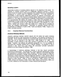 Section 403 Procedural and Monitoring Guidance
Light Microscopy Methods
LM (histologic) methods use the light microscope to view cells and tissues. These
methods can detect changes such as inflammatory responses, alterations in the
appearance of cells, cancerous/precancerous lesions, and damage due to parasites
(USEPA, 1986c). The advantages of LM methods are that they are organ-specific (i.e.,
the lesion can be localized to a specific organ) and can detect microscopic and subtle
cellular alterations that are not evident on visual inspection. However, LM methods are
more expensive (approximately $30/sample) and slower than gross methods.
Electron Microscopy Methods
EM methods use the electron microscope to detect changes in tissue at cellular and
subcellular levels, such as the identification of the nature of inclusion bodies or changes
in the amount of smooth endoplasmic reticulum. An advantage of EM methods is that
they can be highly specific because the pollutant can be localized within certain parts of
the cell. These inclusions may contain the causative chemical agent; lead, gold, iron,
bismuth, uranium, beryllium, mercury, copper, and arsenic are a few of the metals that
can be deposited intracellularly (Sorenson and Smith, 1981). Additionally, EM methods
can be used to investigate subcellular mechanisms of pollutant action. The major
disadvantage of EM methods is that they are very expensive (minimum $400/fish) and
very slow, requiring highly skilled technical expertise.
Histochemical Methods
Histochemical methods use the microscope in conjunction with special chemical tests
and stains to localize specific enzyme systems or reaction products in the cell. For
instance, histochemical assays have been used on liver tissue during and after tumor
formation to yield important information on the biochemistry of specific lesions (Hinton et
al., 1988; Prophet et al., 1992; Sumner, 1988). Histochemical methods are reliable and
can be highly specific for certain classes of organic compounds and metals. However,
highly skilled technical expertise is required to carry out the methods in the laboratory.
In Vitro Tests
In vitro tests are generally more sensitive than whole animal systems, less expensive to
carry out, and of shorter duration. However, in in vitro tests, defense mechanisms found
in the intact animal are missing. In vitro systems offer the greatest flexibility for the
testing and study of environmental contaminants. They can be designed to be relevant
to the species of interest in a given area, and multiple types of measurements can be
taken from a single test system (e.g., metabolic products, mitotic activity, cytotoxicity
and genetic damage). However, comparative in vitro and in vivo studies are needed to
correlate and relate changes that occur in each system (Landolt and Kocan, 1983).
131
image:
Section 403 Procedural and Monitoring Guidance
Light Microscopy Methods
LM (histologic) methods use the light microscope to view cells and tissues. These
methods can detect changes such as inflammatory responses, alterations in the
appearance of cells, cancerous/precancerous lesions, and damage due to parasites
(USEPA, 1986c). The advantages of LM methods are that they are organ-specific (i.e.,
the lesion can be localized to a specific organ) and can detect microscopic and subtle
cellular alterations that are not evident on visual inspection. However, LM methods are
more expensive (approximately $30/sample) and slower than gross methods.
Electron Microscopy Methods
EM methods use the electron microscope to detect changes in tissue at cellular and
subcellular levels, such as the identification of the nature of inclusion bodies or changes
in the amount of smooth endoplasmic reticulum. An advantage of EM methods is that
they can be highly specific because the pollutant can be localized within certain parts of
the cell. These inclusions may contain the causative chemical agent; lead, gold, iron,
bismuth, uranium, beryllium, mercury, copper, and arsenic are a few of the metals that
can be deposited intracellularly (Sorenson and Smith, 1981). Additionally, EM methods
can be used to investigate subcellular mechanisms of pollutant action. The major
disadvantage of EM methods is that they are very expensive (minimum $400/fish) and
very slow, requiring highly skilled technical expertise.
Histochemical Methods
Histochemical methods use the microscope in conjunction with special chemical tests
and stains to localize specific enzyme systems or reaction products in the cell. For
instance, histochemical assays have been used on liver tissue during and after tumor
formation to yield important information on the biochemistry of specific lesions (Hinton et
al., 1988; Prophet et al., 1992; Sumner, 1988). Histochemical methods are reliable and
can be highly specific for certain classes of organic compounds and metals. However,
highly skilled technical expertise is required to carry out the methods in the laboratory.
In Vitro Tests
In vitro tests are generally more sensitive than whole animal systems, less expensive to
carry out, and of shorter duration. However, in in vitro tests, defense mechanisms found
in the intact animal are missing. In vitro systems offer the greatest flexibility for the
testing and study of environmental contaminants. They can be designed to be relevant
to the species of interest in a given area, and multiple types of measurements can be
taken from a single test system (e.g., metabolic products, mitotic activity, cytotoxicity
and genetic damage). However, comparative in vitro and in vivo studies are needed to
correlate and relate changes that occur in each system (Landolt and Kocan, 1983).
131
image:
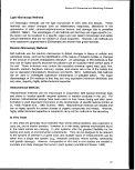 Methods
Reproductive/Developmental Methods
Reproduction studies are designed to examine a number of parameters in the
reproductive process: gross examination of the egg and numbers of eggs, embryo
viability, the proportion of fertilized eggs (i.e., fertilization success), and larval
development and viability (USEPA, 1986c). Studies that examine the egg itself
incorporate microscopic methods that are time-consuming and expensive (West, 1990),
but serve as a direct measure of reproductive success. Some methods deal with the
egg at the molecular level and analyze the action of chemical and physical agents
whose toxicity is directed toward genetic (DNA) components of the egg.
Different cytogenotoxic tests can be used to measure a diverse array of effects including
gene mutation, chromosome damage (sister chromatid exchange), primary DNA
damage, or oncogenesis (i.e., tumor formation and development) (Brusick, 1980;
Landolt and Kocan, 1983; Klingerman, 1982; Shugart, 1990). Another area that is
currently being investigated as a suitable, sublethal assay for toxicity of certain wastes in
the marine environment is the fin regeneration test (Weis et al., 1990). The information
collected using these methods can be used to assess the effects of pollutants on the
reproductive capacity of animals. An understanding of these effects can be useful in
evaluating observed population and community-level changes relative to the occurrence
of specific pollutants.
Gonadotropic and steroidogenic hormones regulate the reproductive capacity of an
organism. The level of these hormones has been used to assess how pollutants affect
the reproductive capacity of fish (V. Varanasi, 1990, National Marine Fisheries Service,
NOAA, personal communication). The analysis is a sensitive indicator of exposure
affecting major biological processes that impact the whole population. However,
relatively detailed information about the normal reproductive cycle of the animals is
necessary to apply these methods in the field (V. Varanasi, 1990, National Marine
Fisheries Service, NOAA, personal communication).
Biochemical Methods
Biochemical methods have been used in field studies to measure various indicators of
environmental contamination. These methods are inherently sensitive and may provide
basic information about early changes in response to environmental contamination at
the cellular level. The development of a suite of indicators having both specific and
nonspecific responses can provide information on the type of stressors, mechanisms of
action, extent of physiological dysfunction, and potential long-term population
consequences (Thomas, 1990).
Fish can respond to generalized stress, contaminants being one type of stress, through
induction (increased synthesis) of stress proteins (Pickering, 1981; Sanders, 1990).
Stress proteins are currently being investigated for use as generalized biochemical
132
image:
Methods
Reproductive/Developmental Methods
Reproduction studies are designed to examine a number of parameters in the
reproductive process: gross examination of the egg and numbers of eggs, embryo
viability, the proportion of fertilized eggs (i.e., fertilization success), and larval
development and viability (USEPA, 1986c). Studies that examine the egg itself
incorporate microscopic methods that are time-consuming and expensive (West, 1990),
but serve as a direct measure of reproductive success. Some methods deal with the
egg at the molecular level and analyze the action of chemical and physical agents
whose toxicity is directed toward genetic (DNA) components of the egg.
Different cytogenotoxic tests can be used to measure a diverse array of effects including
gene mutation, chromosome damage (sister chromatid exchange), primary DNA
damage, or oncogenesis (i.e., tumor formation and development) (Brusick, 1980;
Landolt and Kocan, 1983; Klingerman, 1982; Shugart, 1990). Another area that is
currently being investigated as a suitable, sublethal assay for toxicity of certain wastes in
the marine environment is the fin regeneration test (Weis et al., 1990). The information
collected using these methods can be used to assess the effects of pollutants on the
reproductive capacity of animals. An understanding of these effects can be useful in
evaluating observed population and community-level changes relative to the occurrence
of specific pollutants.
Gonadotropic and steroidogenic hormones regulate the reproductive capacity of an
organism. The level of these hormones has been used to assess how pollutants affect
the reproductive capacity of fish (V. Varanasi, 1990, National Marine Fisheries Service,
NOAA, personal communication). The analysis is a sensitive indicator of exposure
affecting major biological processes that impact the whole population. However,
relatively detailed information about the normal reproductive cycle of the animals is
necessary to apply these methods in the field (V. Varanasi, 1990, National Marine
Fisheries Service, NOAA, personal communication).
Biochemical Methods
Biochemical methods have been used in field studies to measure various indicators of
environmental contamination. These methods are inherently sensitive and may provide
basic information about early changes in response to environmental contamination at
the cellular level. The development of a suite of indicators having both specific and
nonspecific responses can provide information on the type of stressors, mechanisms of
action, extent of physiological dysfunction, and potential long-term population
consequences (Thomas, 1990).
Fish can respond to generalized stress, contaminants being one type of stress, through
induction (increased synthesis) of stress proteins (Pickering, 1981; Sanders, 1990).
Stress proteins are currently being investigated for use as generalized biochemical
132
image:
 Section 403 Procedural and Monitoring Guidance
indicators of stress in fish, chemical-class pollutant indicators, and mode of action
indicators. The methods for detecting stress proteins involve radioisotopic and
immunologic methods that measure the amount of stress protein present after a stress
(i.e., exposure to a pollutant) occurs. At present, cDNA probes are being used
experimentally to measure the correlation between stress and induction of stress
proteins. These methods potentially afford a high degree of sensitivity.
It has been suggested that induction of the fish hepatic microsomal mono-oxygenase
(MO) enzyme could serve as a sensitive biological indicator for certain classes of
chemicals in water (Payne et al., 1987; Kleinow et al., 1987; Lech et al., 1982; Jimenez
et al., 1990; Haux and Forlin, 1988). Metallothioneins (MT) have been under
consideration for use as a monitoring tool for trace environmental metal pollution due to
their induction as a result of exposure to certain metals (Engel and Roesijadi, 1987;
Garvey, 1990; Haux and Forlin, 1988). However, additional scientific research is
required to understand the basic biology of fish before the exact significance of field
studies using these techniques can be ascertained.
A concern when measuring biochemical variables in fish to detect environmental
pollutants is that their exact biological significance is rarely understood. In addition, for
most of the biochemical variables studied, the normal range for a particular fish
population and the factors influencing these variables are often unknown (Neff, 1985).
Even with these limitations, biochemical methods hold considerable promise as
sensitive early indices of exposure to environmental stressors (Thomas, 1990).
However, additional research is needed so that simplified, more cost-effective field
methodologies can be developed.
Immunoloaical Methods
Immunological biomarkers are simple, sensitive, reproducible, and workable in the field
(Weeks et al., 1990; D. Anderson, 1990; R.S. Anderson, 1990). These indicators
provide supportive evidence for linkage between a stressor (toxicant, etc.) and disease
outbreaks in fish and shellfish. The immune response can be used to monitor a specific
antigen or microorganism responsible for pathological conditions in fish. Biologists can
perform quick and sensitive assays in the field or in their own diagnostic laboratories
because many immune assays are becoming available in kits (Rowley, 1990; Matthews
et al., 1990). Many immunological assays do not require sacrifice of the animal. Blood
samples can be taken periodically to follow the kinetics of the effects of stress in a single
animal; however, the effects of handling stress on aquatic species must also be
considered in this case. The immune response is physiologically similar among most
vertebrates and similar equipment and materials can be used to test all species of fish
as well as shellfish (see Anderson, 1987). There is a rapidly growing body of literature
on immunotoxicology from veterinary and aquatic animal sciences.
133
image:
Section 403 Procedural and Monitoring Guidance
indicators of stress in fish, chemical-class pollutant indicators, and mode of action
indicators. The methods for detecting stress proteins involve radioisotopic and
immunologic methods that measure the amount of stress protein present after a stress
(i.e., exposure to a pollutant) occurs. At present, cDNA probes are being used
experimentally to measure the correlation between stress and induction of stress
proteins. These methods potentially afford a high degree of sensitivity.
It has been suggested that induction of the fish hepatic microsomal mono-oxygenase
(MO) enzyme could serve as a sensitive biological indicator for certain classes of
chemicals in water (Payne et al., 1987; Kleinow et al., 1987; Lech et al., 1982; Jimenez
et al., 1990; Haux and Forlin, 1988). Metallothioneins (MT) have been under
consideration for use as a monitoring tool for trace environmental metal pollution due to
their induction as a result of exposure to certain metals (Engel and Roesijadi, 1987;
Garvey, 1990; Haux and Forlin, 1988). However, additional scientific research is
required to understand the basic biology of fish before the exact significance of field
studies using these techniques can be ascertained.
A concern when measuring biochemical variables in fish to detect environmental
pollutants is that their exact biological significance is rarely understood. In addition, for
most of the biochemical variables studied, the normal range for a particular fish
population and the factors influencing these variables are often unknown (Neff, 1985).
Even with these limitations, biochemical methods hold considerable promise as
sensitive early indices of exposure to environmental stressors (Thomas, 1990).
However, additional research is needed so that simplified, more cost-effective field
methodologies can be developed.
Immunoloaical Methods
Immunological biomarkers are simple, sensitive, reproducible, and workable in the field
(Weeks et al., 1990; D. Anderson, 1990; R.S. Anderson, 1990). These indicators
provide supportive evidence for linkage between a stressor (toxicant, etc.) and disease
outbreaks in fish and shellfish. The immune response can be used to monitor a specific
antigen or microorganism responsible for pathological conditions in fish. Biologists can
perform quick and sensitive assays in the field or in their own diagnostic laboratories
because many immune assays are becoming available in kits (Rowley, 1990; Matthews
et al., 1990). Many immunological assays do not require sacrifice of the animal. Blood
samples can be taken periodically to follow the kinetics of the effects of stress in a single
animal; however, the effects of handling stress on aquatic species must also be
considered in this case. The immune response is physiologically similar among most
vertebrates and similar equipment and materials can be used to test all species of fish
as well as shellfish (see Anderson, 1987). There is a rapidly growing body of literature
on immunotoxicology from veterinary and aquatic animal sciences.
133
image:
 Methods
The selection of immune system indicators for the study of stress effects depends on
many factors, including specific study objectives, available equipment, training,
personnel, and length and number of assays. The most sophisticated and sensitive
assays are costly and require highly trained personnel, whereas simple assays can be
performed by field biologists with only basic laboratory supplies.
A major limitation of immune indicators is that the response is sometimes too broad to
provide conclusive evidence that the observed reaction is actually due to a specific
complex to be considered. Cross-reactions and heightened responses to nonspecific
factors may prevent the interpretation of assays with absolute certainty. The immune
response in fish or shellfish will be distinctive for a specific antigen or disease-causing
agent. This will frequently make it difficult to know which immune indicator is most
affected and which immunological assay to apply. Expensive materials and laboratory
equipment are needed for sophisticated immunological assays. Confirmatory assays
are advisable to be sure that a particular stressor is the only cause of a particular effect.
Many animals should be sampled because of natural variability among individuals.
Physiological Methods
Hematological methods have been used by biologists for many years to assess the
general health of fish in hatcheries and research laboratories. The procedures are
well-standardized (Blaxhall and Daisley, 1973; Wedemeyer and Yasutake, 1977) and
are easy to carry out, even in the field. Hematological measures may be affected by the
stress of capture, but are far less influenced than some other measurements, such as
blood glucose (Larson et al., 1985). Hematologic methods have been successfully
implemented in the field and have been rated as the best physiologic method for
evaluation of pollutants (U.S. EPA, 1986c). For the measurement of hematological
factors in fish, techniques similar to those used in human and veterinary clinical
laboratories are generally used with minor modifications (Heath, 1987; Bouck 1984).
Blaxhall and Daisley (1973), Wedemeyer and Yasutake (1977), and Ellis (1977) provide
practical guides to the adaptation of these methods for use on fish blood.
The hematocrii/erythrocyte determination may not be as sensitive to pollution as is the
leucocyte count, at least as far as its response to metals is concerned (Larson et al.,
1985). It remains to be determined how sensitive the procedure is to subtle
environmental changes. In general, chemical and physical stressors cause a decrease
in the leucocrit, whereas infections produce the opposite response. However, it is also
possible to obtain elevations in granulocytes concomitant with a decrease in
lymphocytes, thereby yielding an unchanged leucocrit (Peters et al., 1980). Thus, the
method has limitations for the detection of chronic stress (Wedemeyer et al., 1983).
t
Several obstacles, such as capture stress, limit the potential usefulness of physiological
tests in field work. Capture stress precludes the use of sensitive, early indicators of
environmental stress. The use of physiological responses of wild fish to assess
134
image:
Methods
The selection of immune system indicators for the study of stress effects depends on
many factors, including specific study objectives, available equipment, training,
personnel, and length and number of assays. The most sophisticated and sensitive
assays are costly and require highly trained personnel, whereas simple assays can be
performed by field biologists with only basic laboratory supplies.
A major limitation of immune indicators is that the response is sometimes too broad to
provide conclusive evidence that the observed reaction is actually due to a specific
complex to be considered. Cross-reactions and heightened responses to nonspecific
factors may prevent the interpretation of assays with absolute certainty. The immune
response in fish or shellfish will be distinctive for a specific antigen or disease-causing
agent. This will frequently make it difficult to know which immune indicator is most
affected and which immunological assay to apply. Expensive materials and laboratory
equipment are needed for sophisticated immunological assays. Confirmatory assays
are advisable to be sure that a particular stressor is the only cause of a particular effect.
Many animals should be sampled because of natural variability among individuals.
Physiological Methods
Hematological methods have been used by biologists for many years to assess the
general health of fish in hatcheries and research laboratories. The procedures are
well-standardized (Blaxhall and Daisley, 1973; Wedemeyer and Yasutake, 1977) and
are easy to carry out, even in the field. Hematological measures may be affected by the
stress of capture, but are far less influenced than some other measurements, such as
blood glucose (Larson et al., 1985). Hematologic methods have been successfully
implemented in the field and have been rated as the best physiologic method for
evaluation of pollutants (U.S. EPA, 1986c). For the measurement of hematological
factors in fish, techniques similar to those used in human and veterinary clinical
laboratories are generally used with minor modifications (Heath, 1987; Bouck 1984).
Blaxhall and Daisley (1973), Wedemeyer and Yasutake (1977), and Ellis (1977) provide
practical guides to the adaptation of these methods for use on fish blood.
The hematocrii/erythrocyte determination may not be as sensitive to pollution as is the
leucocyte count, at least as far as its response to metals is concerned (Larson et al.,
1985). It remains to be determined how sensitive the procedure is to subtle
environmental changes. In general, chemical and physical stressors cause a decrease
in the leucocrit, whereas infections produce the opposite response. However, it is also
possible to obtain elevations in granulocytes concomitant with a decrease in
lymphocytes, thereby yielding an unchanged leucocrit (Peters et al., 1980). Thus, the
method has limitations for the detection of chronic stress (Wedemeyer et al., 1983).
t
Several obstacles, such as capture stress, limit the potential usefulness of physiological
tests in field work. Capture stress precludes the use of sensitive, early indicators of
environmental stress. The use of physiological responses of wild fish to assess
134
image:
 Section 403 Procedural and Monitoring Guidance
environmental quality is difficult because responses due to toxicants often cannot be
distinguished from those induced during handling of the wild fish (Bouck, 1984; Folmar,
1993).
4.6.4 QA/QC Considerations
Pathobiological methods have a wide range of sensitivities and response times (i.e.,
when a response can be detected). For instance, certain immunologic, electron
microscopic, and biochemical methods can detect early changes in cells and are very
sensitive. Gross anatomic pathology methods, on the other hand, can detect cellular
changes only after lesions can be seen and, therefore, are less sensitive.
General considerations for QA/QC procedures have been covered earlier in this
document. With regard to pathobiological methods, it should be noted that careful and
consistent handling of aquatic specimens is required to minimize trauma and
confounding effects, such as exposure to air. Organisms should be held in the
laboratory under conditions as near to those found at the site of collection as possible
and for as short a time as practicable before performing assays. Fish and shellfish
collected for histopathological examination must be properly fixed (e.g., immersed in a
formaldehyde or glutaraldehyde solution) to stop metabolic activity. This may require
opening or sectioning the organisms to allow the fixative to rapidly penetrate all tissues
and preserve the cellular structure in its existing condition. The organisms must still be
active or moribund, but not dead, before being fixed. Failure to follow proper fixation
procedures will interfere with the interpretation of lesions in anatomic pathology studies.
As with other monitoring methods, samples must be accurately labeled at the time of
collection and routine QA/QC procedures should be instituted, including tracking
samples, carefully recording methods used, using fresh solutions, and treating both
control and exposed samples equally. Whenever possible, organisms for each group to
be tested should be of the same species, age, and sex. Sections of tissues and organs,
or for small organisms, the whole animal, should also be prepared as uniformly as
possible with respect to homogeneity and orientation so that microscopic observations
can be made on the same organs and areas for each specimen. Subsamples of
sections should be examined (blind) by another pathologist to confirm the diagnoses.
See USEPA (1987b) for additional information on QA/QC procedures for
histopathological examinations.
4.6.5 Statistical Design Considerations
Statistical strategies may mitigate the high costs of pathobiological monitoring methods.
As discussed earlier, power analyses considering the strategy of compositing samples
can often lead to a cost-effective monitoring design strategy. Power-cost analyses are
necessary in selecting the appropriate sample/replicate number, sample location, and
sampling frequency. If the primary objective of a monitoring program is to determine
135
image:
Section 403 Procedural and Monitoring Guidance
environmental quality is difficult because responses due to toxicants often cannot be
distinguished from those induced during handling of the wild fish (Bouck, 1984; Folmar,
1993).
4.6.4 QA/QC Considerations
Pathobiological methods have a wide range of sensitivities and response times (i.e.,
when a response can be detected). For instance, certain immunologic, electron
microscopic, and biochemical methods can detect early changes in cells and are very
sensitive. Gross anatomic pathology methods, on the other hand, can detect cellular
changes only after lesions can be seen and, therefore, are less sensitive.
General considerations for QA/QC procedures have been covered earlier in this
document. With regard to pathobiological methods, it should be noted that careful and
consistent handling of aquatic specimens is required to minimize trauma and
confounding effects, such as exposure to air. Organisms should be held in the
laboratory under conditions as near to those found at the site of collection as possible
and for as short a time as practicable before performing assays. Fish and shellfish
collected for histopathological examination must be properly fixed (e.g., immersed in a
formaldehyde or glutaraldehyde solution) to stop metabolic activity. This may require
opening or sectioning the organisms to allow the fixative to rapidly penetrate all tissues
and preserve the cellular structure in its existing condition. The organisms must still be
active or moribund, but not dead, before being fixed. Failure to follow proper fixation
procedures will interfere with the interpretation of lesions in anatomic pathology studies.
As with other monitoring methods, samples must be accurately labeled at the time of
collection and routine QA/QC procedures should be instituted, including tracking
samples, carefully recording methods used, using fresh solutions, and treating both
control and exposed samples equally. Whenever possible, organisms for each group to
be tested should be of the same species, age, and sex. Sections of tissues and organs,
or for small organisms, the whole animal, should also be prepared as uniformly as
possible with respect to homogeneity and orientation so that microscopic observations
can be made on the same organs and areas for each specimen. Subsamples of
sections should be examined (blind) by another pathologist to confirm the diagnoses.
See USEPA (1987b) for additional information on QA/QC procedures for
histopathological examinations.
4.6.5 Statistical Design Considerations
Statistical strategies may mitigate the high costs of pathobiological monitoring methods.
As discussed earlier, power analyses considering the strategy of compositing samples
can often lead to a cost-effective monitoring design strategy. Power-cost analyses are
necessary in selecting the appropriate sample/replicate number, sample location, and
sampling frequency. If the primary objective of a monitoring program is to determine
135
image:
 Methods
pathobiological differences between sampling locations, composite sampling may be an
appropriate strategy. However, a limitation of composite sampling is the inability to
directly estimate the range and variance of the population of individual samples.
Similarly, the use of space- or time-bulking strategies will severely limit a monitoring
program's ability to assess spatial and temporal heterogeneity of the samples.
Given that the monitoring program must accommodate a fixed level of sampling cost,
the best strategy for pathobiological monitoring is to collect more replicates at fewer
locations. For histopathology, from 25 to 100 animals per species may need to be
surveyed to detect low incidences of disease. The selection of appropriate statistical
analyses must be made with these limitations in mind, as well as the specific types of
statistical analyses that can be performed on different types of data. For example,
quantitative information from measurements of enzyme levels or computerized image
analysis/morphometric programs may be effectively analyzed by parametric statistics (if
the data fit the conditions for normal distributions, limitations of assumptions, etc.), but
histopathological observations may need to be rated on presence/absence or
categorized qualitative scales that will require nonparametric techniques. USEPA
(1987b) provides additional information on the types of sampling designs and statistical
tests that may be appropriate for these data.
4.6.6
Use of Data
Data Interpretation
Data interpretation for pathobiological methods may be limited because there are
relatively few trained personnel, facilities and equipment may be expensive, and
references for newly emerging techniques may be scarce. However, because of the
recent interest in developing biomarkers for monitoring the effects of natural and
anthropogenic environmental stresses on aquatic organisms, many research programs
are under way at Federal, State, and academic facilities to develop, standardize, and
validate the most promising biomarkers for sentinel species that will establish
cause-and-effect links for pollutant exposure. Basic laboratory research and
experimental studies must be conducted in conjunction with field work to elucidate the
relationships between contaminant levels, structural, biochemical, or functional
pathologies, and population health (Johnson and Bergman, 1984; McCarthy, 1990). A
critical concern is the coordination of efforts and creation of a multidisciplinary approach.
It is important to establish baseline data on selected species, as well as to demonstrate
the alterations in the health of those species due to contaminant exposures. Methods
and techniques, terminology, and interpretation of lesions and effects must be
standardized. In addition to a rapidly expanding body of literature on baseline measures
of health, histological atlases for several species of fish and shellfish, and courses,
workshops, meetings, and special symposia (e.g., Responses of Marine Organisms to
Pollutants/Woods Hole, MA, and Plymouth, England; Annual Aquatic Toxicology
136
image:
Methods
pathobiological differences between sampling locations, composite sampling may be an
appropriate strategy. However, a limitation of composite sampling is the inability to
directly estimate the range and variance of the population of individual samples.
Similarly, the use of space- or time-bulking strategies will severely limit a monitoring
program's ability to assess spatial and temporal heterogeneity of the samples.
Given that the monitoring program must accommodate a fixed level of sampling cost,
the best strategy for pathobiological monitoring is to collect more replicates at fewer
locations. For histopathology, from 25 to 100 animals per species may need to be
surveyed to detect low incidences of disease. The selection of appropriate statistical
analyses must be made with these limitations in mind, as well as the specific types of
statistical analyses that can be performed on different types of data. For example,
quantitative information from measurements of enzyme levels or computerized image
analysis/morphometric programs may be effectively analyzed by parametric statistics (if
the data fit the conditions for normal distributions, limitations of assumptions, etc.), but
histopathological observations may need to be rated on presence/absence or
categorized qualitative scales that will require nonparametric techniques. USEPA
(1987b) provides additional information on the types of sampling designs and statistical
tests that may be appropriate for these data.
4.6.6
Use of Data
Data Interpretation
Data interpretation for pathobiological methods may be limited because there are
relatively few trained personnel, facilities and equipment may be expensive, and
references for newly emerging techniques may be scarce. However, because of the
recent interest in developing biomarkers for monitoring the effects of natural and
anthropogenic environmental stresses on aquatic organisms, many research programs
are under way at Federal, State, and academic facilities to develop, standardize, and
validate the most promising biomarkers for sentinel species that will establish
cause-and-effect links for pollutant exposure. Basic laboratory research and
experimental studies must be conducted in conjunction with field work to elucidate the
relationships between contaminant levels, structural, biochemical, or functional
pathologies, and population health (Johnson and Bergman, 1984; McCarthy, 1990). A
critical concern is the coordination of efforts and creation of a multidisciplinary approach.
It is important to establish baseline data on selected species, as well as to demonstrate
the alterations in the health of those species due to contaminant exposures. Methods
and techniques, terminology, and interpretation of lesions and effects must be
standardized. In addition to a rapidly expanding body of literature on baseline measures
of health, histological atlases for several species of fish and shellfish, and courses,
workshops, meetings, and special symposia (e.g., Responses of Marine Organisms to
Pollutants/Woods Hole, MA, and Plymouth, England; Annual Aquatic Toxicology
136
image:
 Section 403 Procedural and Monitoring Guidance
Workshop, Canada), several professional societies (e.g., Society for Invertebrate
Pathology, American Fisheries Society/Fish Health Section) are facilitating training in
techniques and communication among investigators and laboratories. Diseases of fish
and shellfish have been reviewed by several authors (e.g., Sparks, 1985; Ferguson,
1989; Roberts, 1989; Sindermann, 1990; Couch and Fournie, 1993). For
histopathological studies of tumors in fish, standardization of nomenclature will be
available in Dawe et al. (in press).
As for any monitoring program, long-term studies of health and disease in aquatic
organisms will aid in identifying and interpreting observed pathobiological effects.
Furthermore, it will be important to archive data so that they will be available for future
comparisons. The Registry of Tumors in Lower Animals at the National Museum of
Natural History, Smithsonian Institution, Washington, DC, houses over 3,500 cases of
neoplastic and nonneoplastic lesions representing a wide variety of host aquatic
species, pathogens, and environmental stresses from field and laboratory studies
conducted around the world. The Registry also contains the Registry of Marine
Pathology, originally developed by the National Marine Fisheries Service (NMFS), and
the collection of crustacean histopathological material researched by Dr. Phyllis T.
Johnson, NMFS. Although primarily serving as a clearinghouse for information on
neoplastic diseases and research, the Registry is also able to direct inquiries for
information on nonneoplastic diseases, and the materials archived there are available
for study by qualified investigators. Data collected from the long-term monitoring efforts
of NOAA's National Status and Trends Program (NS&T) and EPA's Environmental
Monitoring and Assessment Program (EMAP) will also provide useful information for the
interpretation of the various pathobiological methods that are being employed in these
studies.
Data Integration
Measuring or evaluating the effects of stressors on fish and shellfish by pathobiological
indicators is difficult primarily because of the large number of variables that can
influence biological response. Variables including water temperature, nutritional status,
species, sex, reproductive and developmental stages, and physiological functions can
render tests difficult to compare and evaluate.
Anderson (1990) outlined a plan including four levels of study in a tiered approach to
investigate the effects of stress on the immune system and to quantify the possible
contribution of these environmental and physiological variables on the stress response.
The plan, generally speaking, appears to be applicable to all pathobiological methods
and may be adapted to them using the following four levels: (1) observations of fish and
shellfish populations in the field; (2) studies of caged fish or shellfish in the field; (3) in
vivo exposures in the laboratory; and (4) in vitro assays in the laboratory.
137
image:
Section 403 Procedural and Monitoring Guidance
Workshop, Canada), several professional societies (e.g., Society for Invertebrate
Pathology, American Fisheries Society/Fish Health Section) are facilitating training in
techniques and communication among investigators and laboratories. Diseases of fish
and shellfish have been reviewed by several authors (e.g., Sparks, 1985; Ferguson,
1989; Roberts, 1989; Sindermann, 1990; Couch and Fournie, 1993). For
histopathological studies of tumors in fish, standardization of nomenclature will be
available in Dawe et al. (in press).
As for any monitoring program, long-term studies of health and disease in aquatic
organisms will aid in identifying and interpreting observed pathobiological effects.
Furthermore, it will be important to archive data so that they will be available for future
comparisons. The Registry of Tumors in Lower Animals at the National Museum of
Natural History, Smithsonian Institution, Washington, DC, houses over 3,500 cases of
neoplastic and nonneoplastic lesions representing a wide variety of host aquatic
species, pathogens, and environmental stresses from field and laboratory studies
conducted around the world. The Registry also contains the Registry of Marine
Pathology, originally developed by the National Marine Fisheries Service (NMFS), and
the collection of crustacean histopathological material researched by Dr. Phyllis T.
Johnson, NMFS. Although primarily serving as a clearinghouse for information on
neoplastic diseases and research, the Registry is also able to direct inquiries for
information on nonneoplastic diseases, and the materials archived there are available
for study by qualified investigators. Data collected from the long-term monitoring efforts
of NOAA's National Status and Trends Program (NS&T) and EPA's Environmental
Monitoring and Assessment Program (EMAP) will also provide useful information for the
interpretation of the various pathobiological methods that are being employed in these
studies.
Data Integration
Measuring or evaluating the effects of stressors on fish and shellfish by pathobiological
indicators is difficult primarily because of the large number of variables that can
influence biological response. Variables including water temperature, nutritional status,
species, sex, reproductive and developmental stages, and physiological functions can
render tests difficult to compare and evaluate.
Anderson (1990) outlined a plan including four levels of study in a tiered approach to
investigate the effects of stress on the immune system and to quantify the possible
contribution of these environmental and physiological variables on the stress response.
The plan, generally speaking, appears to be applicable to all pathobiological methods
and may be adapted to them using the following four levels: (1) observations of fish and
shellfish populations in the field; (2) studies of caged fish or shellfish in the field; (3) in
vivo exposures in the laboratory; and (4) in vitro assays in the laboratory.
137
image:
 Methods
The first level of study includes the collection of information from field observations on
relative abundance, reduction in sport-fish catches, or decline in commercial harvests.
Reduced yields reported by anglers in previously productive fishing grounds may be
correlated with environmental stressors or pollutants occurring at these sites. If sick or
moribund fish or shellfish are called to the attention of local biologists by anglers, gross
morphological descriptions might be made and isolation of the disease agent attempted.
The second level of investigation involves the use of caged fish or shellfish placed in the
field to test for the presence or action of environmental stressors. Groups of fish or
shellfish can be placed in pens or cages at suspected sites and their responses (signs of
disease, acute mortality) can be compared with those of control fish or shellfish caged in
unstressful areas. Organisms from the cages can be sampled at various intervals and
the intensity of various immune responses quantified as a function of the time the fish or
shellfish were exposed. Levels of immune responses can be compared by injecting
specific disease agents into both control and test organisms, and recording disease and
death rates.
The third level of assay is in vivo laboratory tests, by which immune response can be
evaluated in experiments with calibrated dilutions of specific contaminants and kinetic
measurements of the immune response at each dilution. Challenges with disease
agents can be more easily controlled in the laboratory to provide information on how the
stressor makes the fish or shellfish more susceptible to specific pathogens.
A fourth level of investigation is the recently developed method for testing the effects of
chemicals, drugs, and other stressors in vitro. Spleens and other immunopoietic organs
can be removed from fish and placed in tissue culture media and their reactions to
pollutants tested using the passive hemolytic plaque assay (Anderson et al., 1986). Use
of this method to measure the effects of stressors allows maximal control of the levels of
pollutants. Because the immune response is monitored under defined laboratory and
environmental conditions, important information is obtained about how specific stressors
affect the immune response. In vitro methods require fewer fish than in vivo methods
because tissue and organ samples can be divided into many sections, which also
reduces the variability of responses.
McCarthy (1990) presented a research strategy to validate biomarkers and provide the
scientific understanding necessary to interpret biomarker responses. An evolving
monitoring program was proposed that focused broadly on evaluation of contamination
in an array of ecosystem types. The challenges and obstacles to be addressed in such
a program include the following:
• The quantitative and qualitative relationships between chemical exposure,
biomarker response, and adverse effects must be established.
138
image:
Methods
The first level of study includes the collection of information from field observations on
relative abundance, reduction in sport-fish catches, or decline in commercial harvests.
Reduced yields reported by anglers in previously productive fishing grounds may be
correlated with environmental stressors or pollutants occurring at these sites. If sick or
moribund fish or shellfish are called to the attention of local biologists by anglers, gross
morphological descriptions might be made and isolation of the disease agent attempted.
The second level of investigation involves the use of caged fish or shellfish placed in the
field to test for the presence or action of environmental stressors. Groups of fish or
shellfish can be placed in pens or cages at suspected sites and their responses (signs of
disease, acute mortality) can be compared with those of control fish or shellfish caged in
unstressful areas. Organisms from the cages can be sampled at various intervals and
the intensity of various immune responses quantified as a function of the time the fish or
shellfish were exposed. Levels of immune responses can be compared by injecting
specific disease agents into both control and test organisms, and recording disease and
death rates.
The third level of assay is in vivo laboratory tests, by which immune response can be
evaluated in experiments with calibrated dilutions of specific contaminants and kinetic
measurements of the immune response at each dilution. Challenges with disease
agents can be more easily controlled in the laboratory to provide information on how the
stressor makes the fish or shellfish more susceptible to specific pathogens.
A fourth level of investigation is the recently developed method for testing the effects of
chemicals, drugs, and other stressors in vitro. Spleens and other immunopoietic organs
can be removed from fish and placed in tissue culture media and their reactions to
pollutants tested using the passive hemolytic plaque assay (Anderson et al., 1986). Use
of this method to measure the effects of stressors allows maximal control of the levels of
pollutants. Because the immune response is monitored under defined laboratory and
environmental conditions, important information is obtained about how specific stressors
affect the immune response. In vitro methods require fewer fish than in vivo methods
because tissue and organ samples can be divided into many sections, which also
reduces the variability of responses.
McCarthy (1990) presented a research strategy to validate biomarkers and provide the
scientific understanding necessary to interpret biomarker responses. An evolving
monitoring program was proposed that focused broadly on evaluation of contamination
in an array of ecosystem types. The challenges and obstacles to be addressed in such
a program include the following:
• The quantitative and qualitative relationships between chemical exposure,
biomarker response, and adverse effects must be established.
138
image:
 Section 403 Procedural and Monitoring Guidance
• Responses due to chemical exposure must be distinguishable from natural
sources of variability (e.g., ecological and physiological variables,
species-specific differences, and individual variability) if biomarkers are to be
useful in evaluating contamination.
• The validity of extrapolating between biomarker responses measured in
individual organisms and some higher-level effect at a population or
community level must be established.
• The use of exposure biomarkers in animal surrogates to evaluate the
potential for human exposure should be explored.
The plan is an ambitious multiyear research and development program involving the
formulation of a long-term, interagency, interdisciplinary activity such as the
Environmental Monitoring and Assessment Program (EMAP) by EPA in cooperation with
other Federal agencies.
4.6.7 Summary and Recommendations
Rationale
• Pathobiological methods provide information concerning biological organ
systems that, through an evaluation of organ structure, activity, and function,
can be used to determine adverse effects of pollutants in the environment.
• Pathobiological methods should be used in concert so that cause-and-effect
relationships can be evaluated.
Monitoring Design Considerations
• Sampling stations should be located along a contamination gradient (i.e.,
from highly contaminated to uncontaminated). This type of sampling strategy
will allow dose-response relationships to be evaluated.
• Fish pathobiological monitoring should be conducted only if the target
species could reasonably be expected to have spent a considerable amount
of time within the area of contamination.
• Large sample sizes will frequently be required for fish pathobiological
monitoring due to natural variability among individuals and taxa.
Existing Analytical Methods
Anatomic Pathology Methods
• Tissues are examined with the naked eye or the aid of a microscope
139
image:
Section 403 Procedural and Monitoring Guidance
• Responses due to chemical exposure must be distinguishable from natural
sources of variability (e.g., ecological and physiological variables,
species-specific differences, and individual variability) if biomarkers are to be
useful in evaluating contamination.
• The validity of extrapolating between biomarker responses measured in
individual organisms and some higher-level effect at a population or
community level must be established.
• The use of exposure biomarkers in animal surrogates to evaluate the
potential for human exposure should be explored.
The plan is an ambitious multiyear research and development program involving the
formulation of a long-term, interagency, interdisciplinary activity such as the
Environmental Monitoring and Assessment Program (EMAP) by EPA in cooperation with
other Federal agencies.
4.6.7 Summary and Recommendations
Rationale
• Pathobiological methods provide information concerning biological organ
systems that, through an evaluation of organ structure, activity, and function,
can be used to determine adverse effects of pollutants in the environment.
• Pathobiological methods should be used in concert so that cause-and-effect
relationships can be evaluated.
Monitoring Design Considerations
• Sampling stations should be located along a contamination gradient (i.e.,
from highly contaminated to uncontaminated). This type of sampling strategy
will allow dose-response relationships to be evaluated.
• Fish pathobiological monitoring should be conducted only if the target
species could reasonably be expected to have spent a considerable amount
of time within the area of contamination.
• Large sample sizes will frequently be required for fish pathobiological
monitoring due to natural variability among individuals and taxa.
Existing Analytical Methods
Anatomic Pathology Methods
• Tissues are examined with the naked eye or the aid of a microscope
139
image:
 Methods
• Light microscopic (LM) methods
- detect changes at the cellular level
- organ and time-series specific
• Electron microscopic (EM) methods
- detect subcellular changes
- specific as to area of cell or site of pollutant action
• Histochemical methods
- detect enzyme systems or reaction products in the cell
- specific to chemical class
Reproduction/Development Methods
• Reproductive capacity is reflected in population recruitment and abundance
. Methods that examine the egg itself provide a direct measure of reproductive
effects from pollutants
• Cytogenetic (DNA) tests
- in vitro tests offer greatest flexibility in terms of sensitivity, expense, and
time required and are frequently conducted for convenience and
availability.
- sister-chromatid exchange (SCE) assays are DNA damage tests used as
a screening tool and are dose-responsive and sensitive to low
concentrations of pollutants.
- the aneuploidy technique is simple and easy to use but is inaccurate for
sublethal effects.
Biochemical Methods
• Several methods are specific for a certain compound class.
• Use a suite of indicators for environmental monitoring.
• Microsomal mono-oxygenase (MO) assays could serve as sensitive
biological indicators for certain chemical classes.
• Metallothionein (MT) assays are nonspecific for metal exposure, but can
provide information on the likelihood of a particular metal pool producing a
pathological effect.
• Stress proteins are not pollutant-specific, but could result from generalized
stress.
140
image:
Methods
• Light microscopic (LM) methods
- detect changes at the cellular level
- organ and time-series specific
• Electron microscopic (EM) methods
- detect subcellular changes
- specific as to area of cell or site of pollutant action
• Histochemical methods
- detect enzyme systems or reaction products in the cell
- specific to chemical class
Reproduction/Development Methods
• Reproductive capacity is reflected in population recruitment and abundance
. Methods that examine the egg itself provide a direct measure of reproductive
effects from pollutants
• Cytogenetic (DNA) tests
- in vitro tests offer greatest flexibility in terms of sensitivity, expense, and
time required and are frequently conducted for convenience and
availability.
- sister-chromatid exchange (SCE) assays are DNA damage tests used as
a screening tool and are dose-responsive and sensitive to low
concentrations of pollutants.
- the aneuploidy technique is simple and easy to use but is inaccurate for
sublethal effects.
Biochemical Methods
• Several methods are specific for a certain compound class.
• Use a suite of indicators for environmental monitoring.
• Microsomal mono-oxygenase (MO) assays could serve as sensitive
biological indicators for certain chemical classes.
• Metallothionein (MT) assays are nonspecific for metal exposure, but can
provide information on the likelihood of a particular metal pool producing a
pathological effect.
• Stress proteins are not pollutant-specific, but could result from generalized
stress.
140
image:
 Section 403 Procedural and Monitoring Guttfance
Immunologic Methods
• Immunologic assays can provide information on pollutant-induced stress
effects; however, they may require confirmatory assays.
• Many animals should be sampled because of natural variability among
animals.
Physiologic Methods
• Serious "interferences" can be caused by stress induced during collection
and may limit the potential usefulness of physiological tests because effects
of toxicants cannot be distinguished from those induced during handling of
the wild organisms.
• Hematologic methods for fish, such as measurements of hematocrit (packed
cell volume), hemoglobin concentration, erythrocyte count, and leucocyte
count (or volume), can be successfully used. Although the fish are not
immune to stress of capture, hematologic methods are influenced far less
than some other measurements such as blood glucose.
• The leucocrit can be a more sensitive measure of metal pollution than the
hematocrit.
QA/QC Considerations
• Pathobiological methods have a wide range of sensitivities.
• Organisms must be carefully handled and properly prepared for each method.
• The main areas of concern with regard to analytical QA/QC are precision,
accuracy, representativeness, completeness, and comparability.
Statistical Design Considerations
• Composite tissue sampling consists of mixing tissue samples from two or
more individuals collected at a particular location and time.
• Space-bulking (combining composites from several locations) and/or
time-bulking (combining several composites over time from one location)
strategies should be used judiciously since information concerning spatial
and temporal heterogeneity may be lost.
• Power analyses have shown that for a fixed level of sampling effort, a
monitoring program's power is generally increased by collecting more
replicates at fewer locations.
141
image:
Section 403 Procedural and Monitoring Guttfance
Immunologic Methods
• Immunologic assays can provide information on pollutant-induced stress
effects; however, they may require confirmatory assays.
• Many animals should be sampled because of natural variability among
animals.
Physiologic Methods
• Serious "interferences" can be caused by stress induced during collection
and may limit the potential usefulness of physiological tests because effects
of toxicants cannot be distinguished from those induced during handling of
the wild organisms.
• Hematologic methods for fish, such as measurements of hematocrit (packed
cell volume), hemoglobin concentration, erythrocyte count, and leucocyte
count (or volume), can be successfully used. Although the fish are not
immune to stress of capture, hematologic methods are influenced far less
than some other measurements such as blood glucose.
• The leucocrit can be a more sensitive measure of metal pollution than the
hematocrit.
QA/QC Considerations
• Pathobiological methods have a wide range of sensitivities.
• Organisms must be carefully handled and properly prepared for each method.
• The main areas of concern with regard to analytical QA/QC are precision,
accuracy, representativeness, completeness, and comparability.
Statistical Design Considerations
• Composite tissue sampling consists of mixing tissue samples from two or
more individuals collected at a particular location and time.
• Space-bulking (combining composites from several locations) and/or
time-bulking (combining several composites over time from one location)
strategies should be used judiciously since information concerning spatial
and temporal heterogeneity may be lost.
• Power analyses have shown that for a fixed level of sampling effort, a
monitoring program's power is generally increased by collecting more
replicates at fewer locations.
141
image:
 Methods
The appropriate statistical tests must be performed and may vary depending
on the type of data generated.
Use of Data
Data use and interpretation may be limited by relatively few trained personnel
and expensive equipment, but many research and training programs are now
under way at Federal, State, and academic facilities to improve biomarker
methods in sentinel species.
Basic laboratory research must be conducted and biological methods must
be tested in the field.
Information communication
- need to coordinate efforts, communicate, and create a multidisciplinary
approach to relate lab and field studies and establish cause-and-effect
relationships.
Data integration
- long-range research strategies should be followed to validate biomarkers
and provide scientific understanding necessary to interpret biomarker
responses.
142
image:
Methods
The appropriate statistical tests must be performed and may vary depending
on the type of data generated.
Use of Data
Data use and interpretation may be limited by relatively few trained personnel
and expensive equipment, but many research and training programs are now
under way at Federal, State, and academic facilities to improve biomarker
methods in sentinel species.
Basic laboratory research must be conducted and biological methods must
be tested in the field.
Information communication
- need to coordinate efforts, communicate, and create a multidisciplinary
approach to relate lab and field studies and establish cause-and-effect
relationships.
Data integration
- long-range research strategies should be followed to validate biomarkers
and provide scientific understanding necessary to interpret biomarker
responses.
142
image:
 Section 403 Procedural and Monitoring Guidance
4.7
FISH POPULATIONS
The objective of monitoring fish populations is to detect and describe spatial and
temporal changes in the abundance, structure, and function of fish communities. To
attempt to protect and preserve healthy fish from the possible effects of pollutant
discharges, estimates of fish population abundance and detailed knowledge of fish life
histories are required.
Except in the most severe cases, it is usually impossible to directly link pollutant
loadings to stock levels (i.e., there is a poorly established cause-and-effect relationship
between pollution and fish population responses). Natural population fluctuations in
fishery stocks will usually be much greater than effects due to pollution. The effects of
discharges are obvious when fish are killed outright by high concentrations of toxic
substances (Rothschild, 1986). However, these instances are rare compared to the
prevalent situation, in which fish are exposed to lower pollutant levels that may not be
lethal but are thought to be harmful in some sense. Sublethal pollutant loadings can be
expressed in terms of increased body burden of toxicants or greater incidence of various
lesions. The effects of sublethal concentrations on growth, mortality, and reproduction
are not known (Rothschild, 1986) As a result of these limitations, fish population
measurement methodologies require further refinement and field validation before they
can be promoted for regular use in 403 monitoring or permit decisions.
4.7.1
Rationale
Under section 403 of the Clean Water Act, permitters must use 10 guidelines in
determining whether a discharge results in unreasonable degradation or irreparable
harm to the marine environment. Fish population studies have generally not been used
to directly link a source of pollution to observed responses. However, some recent
studies have indicated that selection of resident bottom fish as indicators of pollution can
support other data linking sources of pollution to environmental effects, especially if such
studies are conducted in conjunction with benthic studies and parallels can be drawn
between the two. In addition, such methodologies do address the following three 403
guidelines:
• Composition and vulnerability of potentially exposed biological communities;
• Importance of the receiving water area to the surrounding biological
community; and
• Existing or potential recreational and commercial fishing.
Population effects can include those caused by changed reproductive rates or changed
distribution and migration patterns. Effects of suppressed reproductive rates on
population density have been clearly demonstrated in the diminishing populations of the
striped bass in San Francisco Bay. The suppressed reproductive rates have been
shown to correlate with toxic concentrations in the bay (Whipple et al., 1984). Several
143
image:
Section 403 Procedural and Monitoring Guidance
4.7
FISH POPULATIONS
The objective of monitoring fish populations is to detect and describe spatial and
temporal changes in the abundance, structure, and function of fish communities. To
attempt to protect and preserve healthy fish from the possible effects of pollutant
discharges, estimates of fish population abundance and detailed knowledge of fish life
histories are required.
Except in the most severe cases, it is usually impossible to directly link pollutant
loadings to stock levels (i.e., there is a poorly established cause-and-effect relationship
between pollution and fish population responses). Natural population fluctuations in
fishery stocks will usually be much greater than effects due to pollution. The effects of
discharges are obvious when fish are killed outright by high concentrations of toxic
substances (Rothschild, 1986). However, these instances are rare compared to the
prevalent situation, in which fish are exposed to lower pollutant levels that may not be
lethal but are thought to be harmful in some sense. Sublethal pollutant loadings can be
expressed in terms of increased body burden of toxicants or greater incidence of various
lesions. The effects of sublethal concentrations on growth, mortality, and reproduction
are not known (Rothschild, 1986) As a result of these limitations, fish population
measurement methodologies require further refinement and field validation before they
can be promoted for regular use in 403 monitoring or permit decisions.
4.7.1
Rationale
Under section 403 of the Clean Water Act, permitters must use 10 guidelines in
determining whether a discharge results in unreasonable degradation or irreparable
harm to the marine environment. Fish population studies have generally not been used
to directly link a source of pollution to observed responses. However, some recent
studies have indicated that selection of resident bottom fish as indicators of pollution can
support other data linking sources of pollution to environmental effects, especially if such
studies are conducted in conjunction with benthic studies and parallels can be drawn
between the two. In addition, such methodologies do address the following three 403
guidelines:
• Composition and vulnerability of potentially exposed biological communities;
• Importance of the receiving water area to the surrounding biological
community; and
• Existing or potential recreational and commercial fishing.
Population effects can include those caused by changed reproductive rates or changed
distribution and migration patterns. Effects of suppressed reproductive rates on
population density have been clearly demonstrated in the diminishing populations of the
striped bass in San Francisco Bay. The suppressed reproductive rates have been
shown to correlate with toxic concentrations in the bay (Whipple et al., 1984). Several
143
image:
 Methods
laboratory studies have demonstrated that certain fish can avoid toxics, including DDT,
endrin, and Duroban. There is, however, no proof that fish avoid toxicants in the field. If
they do, "hotspots" would be avoided by such species and the population would suffer
less exposure to toxic effects.
One of the greatest problems in analyzing effects of toxics on populations is separating
direct toxic effects from natural or non-pollution-related variations including climatic
changes and overfishing. Results of population studies must be evaluated together with
measurements of other environmental parameters before any cause-and-effect
relationship can be established.
4.7.2 Monitoring Design Considerations
Specimen collection, analysis, and evaluation of fish community structure and function
are typically time-consuming, labor-intensive, and expensive tasks. A survey vessel
manned by an experienced crew and specially equipped with gear to collect organisms
is required. Expert taxonomists are needed to identify and enumerate collected fish
specimens.
The results of fish monitoring programs can vary substantially depending on the
objectives and corresponding design specifications. The characteristics primarily
responsible for the variability in the results are the following:
• Type of sampling gear,
• Volume sampled, and
• Location and timing of sample collection.
It is essential to understand the effects of these monitoring design characteristics on the
results and to standardize them as much as possible to ensure the comparability of
sampled data. Analyses of power-cost efficiencies are useful in selecting the
appropriate sampling gear and sample processing protocols. Ferraro et al. (1989)
provide an example of power-cost analyses.
Sampling Devices
Sample collection protocols influence all subsequent laboratory and data analysis; it is
key that fish population samples be collected using acceptable and standardized
techniques. Several types of devices can be used to collect fish samples: traps and
cages, passive nets, trawls (active nets), and photographic surveys (Fredette et al.,
1989). Many of these devices selectively sample specific types of fish. Accordingly,
conducting comparisons between data collected using different devices and even
different nets of the same type is inadvisable.
144
image:
Methods
laboratory studies have demonstrated that certain fish can avoid toxics, including DDT,
endrin, and Duroban. There is, however, no proof that fish avoid toxicants in the field. If
they do, "hotspots" would be avoided by such species and the population would suffer
less exposure to toxic effects.
One of the greatest problems in analyzing effects of toxics on populations is separating
direct toxic effects from natural or non-pollution-related variations including climatic
changes and overfishing. Results of population studies must be evaluated together with
measurements of other environmental parameters before any cause-and-effect
relationship can be established.
4.7.2 Monitoring Design Considerations
Specimen collection, analysis, and evaluation of fish community structure and function
are typically time-consuming, labor-intensive, and expensive tasks. A survey vessel
manned by an experienced crew and specially equipped with gear to collect organisms
is required. Expert taxonomists are needed to identify and enumerate collected fish
specimens.
The results of fish monitoring programs can vary substantially depending on the
objectives and corresponding design specifications. The characteristics primarily
responsible for the variability in the results are the following:
• Type of sampling gear,
• Volume sampled, and
• Location and timing of sample collection.
It is essential to understand the effects of these monitoring design characteristics on the
results and to standardize them as much as possible to ensure the comparability of
sampled data. Analyses of power-cost efficiencies are useful in selecting the
appropriate sampling gear and sample processing protocols. Ferraro et al. (1989)
provide an example of power-cost analyses.
Sampling Devices
Sample collection protocols influence all subsequent laboratory and data analysis; it is
key that fish population samples be collected using acceptable and standardized
techniques. Several types of devices can be used to collect fish samples: traps and
cages, passive nets, trawls (active nets), and photographic surveys (Fredette et al.,
1989). Many of these devices selectively sample specific types of fish. Accordingly,
conducting comparisons between data collected using different devices and even
different nets of the same type is inadvisable.
144
image:
 Section 403 Procedural and Monitoring Guidance
Traps and Cages
Traps and cages are usually designed to attract and capture specific organisms. They
are useful in studies examining the activities of a particular target organism in a given
area. Traps and cages provide only qualitative measures of organisms in a particular
area.
Passive Nets and Trawls
Nets vary in their selectivity of the species that are captured and in the efficiency of
retaining captured specimens. The size of the net, its configuration and orientation, and
the avoidance behavior of the target species should be considered when using any net.
The mesh size affects the speed at which the net can be towed, as well as the size of
fish caught. The slower the towing speed, the more likely that some organisms will
either avoid or escape the net. It is highly recommended that the mesh size, net
opening, and duration, direction, and speed of towing be set in order to compare trawls.
In any monitoring program, otter trawl net size must be kept constant to ensure
intercomparison of sampling results.
Passive nets (e.g., gill nets) are deployed at a fixed position; organisms become
entangled or trapped within the netted area. Passive nets are used to collect selected
target species and to provide a qualitative means of sampling fish populations.
Limitations associated with passive nets include: .
• Nets, ordinarily, must remain in place for an extended period of time.
• Deployment and recovery of nets are typically time-consuming processes.
Trawls (active nets) are drawn through the water, and results are more immediate than
those obtained through the use of passive nets. Trawls are typically used to collect
large quantities of fish at various depths (Fredette et al., 1989).
Photographic Surveys
Photographic surveys are effective when the bottom topography is uneven or trawling is
not possible. The utility of photographic surveys is limited by water clarity, difficulties in
identifying species, and fish avoidance of the camera system. In addition, further
studies comparing photographic surveys to trawls are required before comparisons may
be made. This method is also limited by the qualitative nature of the data (Fredette et
al.,1989).
Volume Sampled
Different species of fish have different scales of horizontal and vertical spatial
distribution (Gushing, 1975; Bond, 1979). Costs of laboratory analysis of the sample
increase with increased volume sampled. Analyses of spatial and temporal scale,
145
image:
Section 403 Procedural and Monitoring Guidance
Traps and Cages
Traps and cages are usually designed to attract and capture specific organisms. They
are useful in studies examining the activities of a particular target organism in a given
area. Traps and cages provide only qualitative measures of organisms in a particular
area.
Passive Nets and Trawls
Nets vary in their selectivity of the species that are captured and in the efficiency of
retaining captured specimens. The size of the net, its configuration and orientation, and
the avoidance behavior of the target species should be considered when using any net.
The mesh size affects the speed at which the net can be towed, as well as the size of
fish caught. The slower the towing speed, the more likely that some organisms will
either avoid or escape the net. It is highly recommended that the mesh size, net
opening, and duration, direction, and speed of towing be set in order to compare trawls.
In any monitoring program, otter trawl net size must be kept constant to ensure
intercomparison of sampling results.
Passive nets (e.g., gill nets) are deployed at a fixed position; organisms become
entangled or trapped within the netted area. Passive nets are used to collect selected
target species and to provide a qualitative means of sampling fish populations.
Limitations associated with passive nets include: .
• Nets, ordinarily, must remain in place for an extended period of time.
• Deployment and recovery of nets are typically time-consuming processes.
Trawls (active nets) are drawn through the water, and results are more immediate than
those obtained through the use of passive nets. Trawls are typically used to collect
large quantities of fish at various depths (Fredette et al., 1989).
Photographic Surveys
Photographic surveys are effective when the bottom topography is uneven or trawling is
not possible. The utility of photographic surveys is limited by water clarity, difficulties in
identifying species, and fish avoidance of the camera system. In addition, further
studies comparing photographic surveys to trawls are required before comparisons may
be made. This method is also limited by the qualitative nature of the data (Fredette et
al.,1989).
Volume Sampled
Different species of fish have different scales of horizontal and vertical spatial
distribution (Gushing, 1975; Bond, 1979). Costs of laboratory analysis of the sample
increase with increased volume sampled. Analyses of spatial and temporal scale,
145
image:
 Methods
statistical power, and costs will assist in determining optimal sample volume. It is highly
recommended that a standard sample volume (same tow duration, tow speed, and net
opening area) be analyzed to ensure data comparability (Green, 1979).
Selection of Sampling Period
Fish assemblages are dynamic; the most common temporal patterns observed in fish
communities are those associated with daily activity patterns (diurnal), seasonal
changes, and life history strategies. To minimize energy expenditure, most fishes mimic
the diurnal activities of their prey. These diurnal fluctuations typically occur in the
vertical scale and should be considered to ensure collection of representative samples.
Seasonal variation in fish assemblages may be due to changes in physical, chemical,
and/or biological parameters: i.e., temperature, light transmissivity, dissolved oxygen,
predation, reproductive stage, recruitment, etc.
Given the seasonal variation characteristic of fish assemblages in general, it is
recommended that direct comparisons between samples collected during different
seasons be avoided. Studies investigating interannual variation in the characteristics of
fish communities should be conducted during the same season (preferably the same
month) each year.
4.7.3 Analytical Methods Considerations
There are a variety of approaches to assess the effects of anthropogenic perturbance on
fish communities of the marine environment. These assessment approaches may be
grouped into three categories :
• Biological indices,
• Indicator species, and
• Multivariate analyses.
There has been little consensus among biologists regarding the suitability of various
techniques for describing community characteristics and/or for assessing impacts. A
critical evaluation of the use of biological indices to detect environmental change is
presented in an EPA Technical Support Document (USEPA, 1985d). The indices,
shown in Table 4-22, are evaluated on the basis of the following criteria :
• Biological meaning,
• Ease of interpretation, and
• Sensitivity to community changes due to anthropogenic sources.
The results of these evaluations and additional information on other analytical methods
are summarized below.
146
image:
Methods
statistical power, and costs will assist in determining optimal sample volume. It is highly
recommended that a standard sample volume (same tow duration, tow speed, and net
opening area) be analyzed to ensure data comparability (Green, 1979).
Selection of Sampling Period
Fish assemblages are dynamic; the most common temporal patterns observed in fish
communities are those associated with daily activity patterns (diurnal), seasonal
changes, and life history strategies. To minimize energy expenditure, most fishes mimic
the diurnal activities of their prey. These diurnal fluctuations typically occur in the
vertical scale and should be considered to ensure collection of representative samples.
Seasonal variation in fish assemblages may be due to changes in physical, chemical,
and/or biological parameters: i.e., temperature, light transmissivity, dissolved oxygen,
predation, reproductive stage, recruitment, etc.
Given the seasonal variation characteristic of fish assemblages in general, it is
recommended that direct comparisons between samples collected during different
seasons be avoided. Studies investigating interannual variation in the characteristics of
fish communities should be conducted during the same season (preferably the same
month) each year.
4.7.3 Analytical Methods Considerations
There are a variety of approaches to assess the effects of anthropogenic perturbance on
fish communities of the marine environment. These assessment approaches may be
grouped into three categories :
• Biological indices,
• Indicator species, and
• Multivariate analyses.
There has been little consensus among biologists regarding the suitability of various
techniques for describing community characteristics and/or for assessing impacts. A
critical evaluation of the use of biological indices to detect environmental change is
presented in an EPA Technical Support Document (USEPA, 1985d). The indices,
shown in Table 4-22, are evaluated on the basis of the following criteria :
• Biological meaning,
• Ease of interpretation, and
• Sensitivity to community changes due to anthropogenic sources.
The results of these evaluations and additional information on other analytical methods
are summarized below.
146
image:
 Section 403 Procedural and Monitoring Guidance
Table 4-22. Biological Indices
Index/Method
Biological Characteristic
Measured
Bray-Curtis (Curtis and Peterson, 1978)
Dominance (Swartz et al.,1985)
Number of individuals (USEPA,1985d)
Number of species (USEPA.1985d)
Biomass (USEPA,1985d)
Margalefs SR (Margalef,1969)
J (Pielou,1966)
Shannon-Wiener H' (USEPA,1985d)
Dissimilarity
Community structure
Total abundance
Total taxa
Standing crop
Diversity
Evenness
Diversity
Biological Indices
The number of individuals and the number of species have been used as indicators of
anthropogenic disturbance, as well as other environmental stresses (USEPA, 1985d).
Furthermore, these simple biological indices are less ambiguous and can often be as
informative as diversity indices (USEPA, 1985d; Green, 1979; Hurlbert, 1971).
Measures of biomass have inherent problems in the collection of the data, e.g., loss or
gain of weight due to preservative medium, drying times, or evaporative weight loss.
More complicated indices-e.g., species diversity, species richness, dominance,
evenness-have found varying degrees of acceptance. Because of this, these methods
should be used in conjunction with other assessment methods to help verify results.
Diversity indices, which are measures of the distribution of individuals among species,
have the following limitations (Green, 1984b):
• They often lack biological meaning;
147
image:
Section 403 Procedural and Monitoring Guidance
Table 4-22. Biological Indices
Index/Method
Biological Characteristic
Measured
Bray-Curtis (Curtis and Peterson, 1978)
Dominance (Swartz et al.,1985)
Number of individuals (USEPA,1985d)
Number of species (USEPA.1985d)
Biomass (USEPA,1985d)
Margalefs SR (Margalef,1969)
J (Pielou,1966)
Shannon-Wiener H' (USEPA,1985d)
Dissimilarity
Community structure
Total abundance
Total taxa
Standing crop
Diversity
Evenness
Diversity
Biological Indices
The number of individuals and the number of species have been used as indicators of
anthropogenic disturbance, as well as other environmental stresses (USEPA, 1985d).
Furthermore, these simple biological indices are less ambiguous and can often be as
informative as diversity indices (USEPA, 1985d; Green, 1979; Hurlbert, 1971).
Measures of biomass have inherent problems in the collection of the data, e.g., loss or
gain of weight due to preservative medium, drying times, or evaporative weight loss.
More complicated indices-e.g., species diversity, species richness, dominance,
evenness-have found varying degrees of acceptance. Because of this, these methods
should be used in conjunction with other assessment methods to help verify results.
Diversity indices, which are measures of the distribution of individuals among species,
have the following limitations (Green, 1984b):
• They often lack biological meaning;
147
image:
 Methods
• They are not robust empirical indicators of any important correlates of
environmental health;
• They do not incorporate information on form and function of resident species; and
• They are susceptible to biases associated with well-described taxa.
Even so, species diversity indices are a widely used measure of community structure.
Although diversity may not be able to pinpoint a single problematic discharge in an area
that contains many, it can be an indicator of degraded water quality. Species diversity in
fish communities is noted to increase with increasing distance from a pollution source
(Armstrong et al., 1970; Bechtel and Copeland, 1970; Tsai, 1968). In fact, Bechtel and
Copeland (1970) found a linear relationship between the volume of toxic effluent
entering the Houston Ship Channel and the fish diversity of shallow stations.
The dominance index is a measure of the degree to which one or a few species
dominate the community. The dominance index, herein defined as the minimum
number of species required to account for 75 percent of the total number of individuals,
has been useful in describing community structure (Swartz et al., 1985). Its advantages
are that it is easily calculated, it does not assume an underlying distribution of
individuals among species, and it is statistically testable.
Indicator Species
The evaluation of abundances of individual indicator species is generally informative and
may reduce the cost of the analysis. The absence of pollution-sensitive species and the
enhancement of opportunistic and pollution-tolerant species may assist in defining the
spatial and temporal extent and magnitude of impacts. A preponderance of
unspecialized feeders indicates areas of stress. However, indicator variables must
possess the following characteristics (Green, 1984b):
• They must provide a sufficiently precise and accurate appraisal of:
- species of concern,
- anthropogenic disturbances to communities, and
- presence/absence or magnitude of anthropogenic perturbance to the
ecosystem.
• They must provide a cost-effective and statistically reliable alternative to
monitoring all critical measures of habitat perturbance.
• They must be appropriate for the spatial and temporal scale demanded by
the study objectives.
Further studies of the response patterns of fish species subjected to anthropogenic
perturbations caused by discharges are required in order to select appropriate indicators
of environmental impact. If a suitable indicator species is identified, it is desirable to
148
image:
Methods
• They are not robust empirical indicators of any important correlates of
environmental health;
• They do not incorporate information on form and function of resident species; and
• They are susceptible to biases associated with well-described taxa.
Even so, species diversity indices are a widely used measure of community structure.
Although diversity may not be able to pinpoint a single problematic discharge in an area
that contains many, it can be an indicator of degraded water quality. Species diversity in
fish communities is noted to increase with increasing distance from a pollution source
(Armstrong et al., 1970; Bechtel and Copeland, 1970; Tsai, 1968). In fact, Bechtel and
Copeland (1970) found a linear relationship between the volume of toxic effluent
entering the Houston Ship Channel and the fish diversity of shallow stations.
The dominance index is a measure of the degree to which one or a few species
dominate the community. The dominance index, herein defined as the minimum
number of species required to account for 75 percent of the total number of individuals,
has been useful in describing community structure (Swartz et al., 1985). Its advantages
are that it is easily calculated, it does not assume an underlying distribution of
individuals among species, and it is statistically testable.
Indicator Species
The evaluation of abundances of individual indicator species is generally informative and
may reduce the cost of the analysis. The absence of pollution-sensitive species and the
enhancement of opportunistic and pollution-tolerant species may assist in defining the
spatial and temporal extent and magnitude of impacts. A preponderance of
unspecialized feeders indicates areas of stress. However, indicator variables must
possess the following characteristics (Green, 1984b):
• They must provide a sufficiently precise and accurate appraisal of:
- species of concern,
- anthropogenic disturbances to communities, and
- presence/absence or magnitude of anthropogenic perturbance to the
ecosystem.
• They must provide a cost-effective and statistically reliable alternative to
monitoring all critical measures of habitat perturbance.
• They must be appropriate for the spatial and temporal scale demanded by
the study objectives.
Further studies of the response patterns of fish species subjected to anthropogenic
perturbations caused by discharges are required in order to select appropriate indicators
of environmental impact. If a suitable indicator species is identified, it is desirable to
148
image:
 Section 403 Procedural and Monitoring Guidance
monitor the status and trend of that species' population. This will also be true of certain
species having high economic or public value (e.g., striped bass). A wide variety of
methods can be used to measure the size of fish populations and assess population
structure. These include mark and recapture techniques and various techniques used to
determine population sex and age structure. Nielson and Johnson (1984) and Cailliet et
al. (1986) provide thorough discussions of these techniques and their applications.
Bicker (1975) provides an excellent discussion of methods for the sampling of fish
populations.
Statistical Analyses
Numerical classification encompasses a wide variety of techniques that have been used
in the analysis of fish data to distinguish groups of entities (e.g., sample locations)
according to similarity of attributes (e.g., species). These techniques differ from most
multivariate methods in that no assumptions are made concerning the underlying
distributions of the variables. Detailed descriptions of numerical classification analysis
can be found in Romesburg (1984), Clifford and Stephenson (1975), Boesch (1977),
Sneath and Sokal (1973), arid Anderberg (1973). Boesch (1977) is particularly valuable
as an introduction and guide to the use of numerical classification analysis in marine
environmental studies. Guidance on the interpretation of classification results is
provided in an EPA Technical Support Document (USEPA, 1988d).
Ordination analyses have also been used to reduce the dimensionality of the data set
while maintaining the relationship between similar and dissimilar entities. At present no
single ordination technique has been shown to be clearly superior for the analysis of
biological data (USEPA, 1985d).
Multivariate analyses are effective heuristic tools. They generate visual representations
that often indicate where further analyses ought to be conducted.
Analytical Approach Recommendations
Some of the most informative measures of community structure are the simplest (Table
4-22):
• Number of individuals,
• Number of species,
• Dominance,
• Abundance of pollution-sensitive species, and
• Abundance of opportunistic and pollution-tolerant species.
149
image:
Section 403 Procedural and Monitoring Guidance
monitor the status and trend of that species' population. This will also be true of certain
species having high economic or public value (e.g., striped bass). A wide variety of
methods can be used to measure the size of fish populations and assess population
structure. These include mark and recapture techniques and various techniques used to
determine population sex and age structure. Nielson and Johnson (1984) and Cailliet et
al. (1986) provide thorough discussions of these techniques and their applications.
Bicker (1975) provides an excellent discussion of methods for the sampling of fish
populations.
Statistical Analyses
Numerical classification encompasses a wide variety of techniques that have been used
in the analysis of fish data to distinguish groups of entities (e.g., sample locations)
according to similarity of attributes (e.g., species). These techniques differ from most
multivariate methods in that no assumptions are made concerning the underlying
distributions of the variables. Detailed descriptions of numerical classification analysis
can be found in Romesburg (1984), Clifford and Stephenson (1975), Boesch (1977),
Sneath and Sokal (1973), arid Anderberg (1973). Boesch (1977) is particularly valuable
as an introduction and guide to the use of numerical classification analysis in marine
environmental studies. Guidance on the interpretation of classification results is
provided in an EPA Technical Support Document (USEPA, 1988d).
Ordination analyses have also been used to reduce the dimensionality of the data set
while maintaining the relationship between similar and dissimilar entities. At present no
single ordination technique has been shown to be clearly superior for the analysis of
biological data (USEPA, 1985d).
Multivariate analyses are effective heuristic tools. They generate visual representations
that often indicate where further analyses ought to be conducted.
Analytical Approach Recommendations
Some of the most informative measures of community structure are the simplest (Table
4-22):
• Number of individuals,
• Number of species,
• Dominance,
• Abundance of pollution-sensitive species, and
• Abundance of opportunistic and pollution-tolerant species.
149
image:
 Methods
These indices have proved to be useful over various habitats and regions in assessing
changes in fish population dynamics (USEPA, 1985d). Values of these variables may
be determined from the list of species abundances generated during the taxonomic
identification of collected specimens. Furthermore, the values of these variables may be
easily tested statistically using parametric or nonparametric techniques. It is
recommended that no single index or analytical method be used to assess impacts;
rather, the assessment of impacts should incorporate information that each variable and
method contributes concerning community structure.
Selection of reference sites is key to the evaluation of environmental impact assessment
of point source dischargers. Results of analyses using reference measures provide the
means of comparison by which anthropogenic impacts are detected. It is essential that
selected reference sites exhibit similar habitat characteristics compared to monitoring
program sampling sites. Several reference sites may be required to meet these criteria.
4.7.4 QA/QC Considerations
Sample Collection
Nets should be inspected for wear and tear leading to sample loss.
Taxonomic Identification
A key QA/QC issue is taxonomic standardization. Consistent taxonomic identifications
are achieved through interaction among taxonomists working on each major group.
Participation of the laboratory staff in regional taxonomic standardization programs is
recommended to ensure regional consistency and accuracy of identification.
A sampling of the verified specimens should then be placed in a permanent reference
collection. All specimens in the reference collection should be stored in labeled
containers that are segregated by species and sample. Reference specimens should
be archived alphabetically within major taxonomic groups.
4.7.5 Statistical Design Considerations
Consideration of statistical strategies will mitigate the high costs of collecting and
processing samples. Power-cost analyses are necessary in selecting appropriate
sample/replicate number, sample location, and sampling frequency.
Temporal Stratification of the Data
The time of the year should be controlled or stratified in the design; the use of annual
averages is seldom good practice. Temporal stratification of the data should not be
attempted until sufficient knowledge of long-term natural cycles is attained. Initially,
simple regression analyses may be conducted on seasonally stratified data to identify
150
image:
Methods
These indices have proved to be useful over various habitats and regions in assessing
changes in fish population dynamics (USEPA, 1985d). Values of these variables may
be determined from the list of species abundances generated during the taxonomic
identification of collected specimens. Furthermore, the values of these variables may be
easily tested statistically using parametric or nonparametric techniques. It is
recommended that no single index or analytical method be used to assess impacts;
rather, the assessment of impacts should incorporate information that each variable and
method contributes concerning community structure.
Selection of reference sites is key to the evaluation of environmental impact assessment
of point source dischargers. Results of analyses using reference measures provide the
means of comparison by which anthropogenic impacts are detected. It is essential that
selected reference sites exhibit similar habitat characteristics compared to monitoring
program sampling sites. Several reference sites may be required to meet these criteria.
4.7.4 QA/QC Considerations
Sample Collection
Nets should be inspected for wear and tear leading to sample loss.
Taxonomic Identification
A key QA/QC issue is taxonomic standardization. Consistent taxonomic identifications
are achieved through interaction among taxonomists working on each major group.
Participation of the laboratory staff in regional taxonomic standardization programs is
recommended to ensure regional consistency and accuracy of identification.
A sampling of the verified specimens should then be placed in a permanent reference
collection. All specimens in the reference collection should be stored in labeled
containers that are segregated by species and sample. Reference specimens should
be archived alphabetically within major taxonomic groups.
4.7.5 Statistical Design Considerations
Consideration of statistical strategies will mitigate the high costs of collecting and
processing samples. Power-cost analyses are necessary in selecting appropriate
sample/replicate number, sample location, and sampling frequency.
Temporal Stratification of the Data
The time of the year should be controlled or stratified in the design; the use of annual
averages is seldom good practice. Temporal stratification of the data should not be
attempted until sufficient knowledge of long-term natural cycles is attained. Initially,
simple regression analyses may be conducted on seasonally stratified data to identify
150
image:
 Section 403 Procedural and Monitoring Guidance
monotonic temporal trends. Whether conditions are improving or degrading over time
may be further examined using various statistical time series analyses (e.g., temporal
autocorrelation, spectral analyses).
Statistical Power
Selection of the number of replicates is an important component of program design.
The inherent patchy distribution of fish communities requires collection of sufficient
replicate samples to ensure an accurate description of the area. However, increases in
replication increase sample processing costs. Power analyses assist in the allocation of
sampling resources (stations, replication, and frequency) with regard to program
finances and design.
Power analyses may be applied to determine the appropriate number of sample
replicates required to detect a specified difference (USEPA, 1987d). The number of
replications required to detect a specified minimum difference is a function of the
statistical power and the variance in the data. Power analyses require a priori
knowledge of the variability in the data. A best guess or, preferably, variation observed
in historical data is often used initially in the design of the monitoring program.
To improve the power of a statistical test, while keeping the significance level constant,
the sample size should be increased. Because of constraints in cost and time imposed
by the monitoring program, however, this option may not be available. Power analyses
have shown that for a fixed level of sampling effort, a monitoring program's power is
generally increased by collecting more replicates at fewer locations. The number and
distribution of sampling locations required to evaluate the effectiveness of the monitoring
program will depend on the size and complexity of the discharge and the surrounding
environment.
4.7.6
Use of Data
Monitoring of fish community structure provides a measure of the health of the marine
habitat and can be used as a tool in the evaluation of spatial and temporal effects of
marine discharges. The presence or absence of certain fish is useful in indicating the
condition of the environment. Monitoring of fish communities also provides data
required in the design and validation of fish population dynamics models and the
selection of biological indicators (USEPA, 1990d).
In addition, monitoring of fish communities may directly provide accurate information
essential in assessing the effectiveness of pollution abatement programs. Analyses of
fish communities may be effectively used to monitor long-term change in the receiving
environment (Gushing, 1975).
151
image:
Section 403 Procedural and Monitoring Guidance
monotonic temporal trends. Whether conditions are improving or degrading over time
may be further examined using various statistical time series analyses (e.g., temporal
autocorrelation, spectral analyses).
Statistical Power
Selection of the number of replicates is an important component of program design.
The inherent patchy distribution of fish communities requires collection of sufficient
replicate samples to ensure an accurate description of the area. However, increases in
replication increase sample processing costs. Power analyses assist in the allocation of
sampling resources (stations, replication, and frequency) with regard to program
finances and design.
Power analyses may be applied to determine the appropriate number of sample
replicates required to detect a specified difference (USEPA, 1987d). The number of
replications required to detect a specified minimum difference is a function of the
statistical power and the variance in the data. Power analyses require a priori
knowledge of the variability in the data. A best guess or, preferably, variation observed
in historical data is often used initially in the design of the monitoring program.
To improve the power of a statistical test, while keeping the significance level constant,
the sample size should be increased. Because of constraints in cost and time imposed
by the monitoring program, however, this option may not be available. Power analyses
have shown that for a fixed level of sampling effort, a monitoring program's power is
generally increased by collecting more replicates at fewer locations. The number and
distribution of sampling locations required to evaluate the effectiveness of the monitoring
program will depend on the size and complexity of the discharge and the surrounding
environment.
4.7.6
Use of Data
Monitoring of fish community structure provides a measure of the health of the marine
habitat and can be used as a tool in the evaluation of spatial and temporal effects of
marine discharges. The presence or absence of certain fish is useful in indicating the
condition of the environment. Monitoring of fish communities also provides data
required in the design and validation of fish population dynamics models and the
selection of biological indicators (USEPA, 1990d).
In addition, monitoring of fish communities may directly provide accurate information
essential in assessing the effectiveness of pollution abatement programs. Analyses of
fish communities may be effectively used to monitor long-term change in the receiving
environment (Gushing, 1975).
151
image:
 Methods
Fish serve as effective indicators of overall environmental condition, delineating the
magnitude, spatial extent, and temporal trends of anthropogenic and natural
perturbations to the ecosystem. Monitoring of fish will provide relevant accurate data
fundamental to achieving the objectives of many marine monitoring programs. Such
measurements, however, will not provide information linking specific pollution sources to
observed effects. The results of the fish stock monitoring program can also be unclear
as a result of the mobility of fish and their range of natural fluctuation. The data can be
used to augment other monitoring data to obtain a clearer picture of the discharge
effects.
4.7.7 Summary and Recommendations
Rationale
• The objective is to detect and describe spatial and temporal changes in the
size, structure, and function of fish communities to protect the economic,
recreational, and aesthetic value of the resident fisheries.
• Monitoring provides in situ measures of habitat quality and is a powerful tool
in assessing environmental impact.
Monitoring Design Considerations
• It is recommended that the types of sampling gear, the volume sampled, and
the location and timing of sample collection be consistent to allow for
comparisons among studies.
• To reduce the variation due to seasonal differences, sampling should be
conducted during the same season—preferably the same month—each year.
Analytical Methods Considerations
• It is recommended that simple measures of community structure be used to
assess the condition of the marine fish: number of individuals, number of
species, dominance, abundance of pollution-sensitive species, and
abundance of pollution-tolerant species.
• Indicator species should possess the following characteristics:
- sensitive to perturbances of concern;
- cost-effective and statistically reliable alternative to measuring all species
in a monitoring program;
- statistically reliable indicative measures of habitat perturbance; and
- appropriate for the spatial and temporal scale demanded by the study
objectives.
752
image:
Methods
Fish serve as effective indicators of overall environmental condition, delineating the
magnitude, spatial extent, and temporal trends of anthropogenic and natural
perturbations to the ecosystem. Monitoring of fish will provide relevant accurate data
fundamental to achieving the objectives of many marine monitoring programs. Such
measurements, however, will not provide information linking specific pollution sources to
observed effects. The results of the fish stock monitoring program can also be unclear
as a result of the mobility of fish and their range of natural fluctuation. The data can be
used to augment other monitoring data to obtain a clearer picture of the discharge
effects.
4.7.7 Summary and Recommendations
Rationale
• The objective is to detect and describe spatial and temporal changes in the
size, structure, and function of fish communities to protect the economic,
recreational, and aesthetic value of the resident fisheries.
• Monitoring provides in situ measures of habitat quality and is a powerful tool
in assessing environmental impact.
Monitoring Design Considerations
• It is recommended that the types of sampling gear, the volume sampled, and
the location and timing of sample collection be consistent to allow for
comparisons among studies.
• To reduce the variation due to seasonal differences, sampling should be
conducted during the same season—preferably the same month—each year.
Analytical Methods Considerations
• It is recommended that simple measures of community structure be used to
assess the condition of the marine fish: number of individuals, number of
species, dominance, abundance of pollution-sensitive species, and
abundance of pollution-tolerant species.
• Indicator species should possess the following characteristics:
- sensitive to perturbances of concern;
- cost-effective and statistically reliable alternative to measuring all species
in a monitoring program;
- statistically reliable indicative measures of habitat perturbance; and
- appropriate for the spatial and temporal scale demanded by the study
objectives.
752
image:
 Section 403 Procedural and Monitoring Guidance
• Selection of reference sites is key to the evaluation of environmental impact
due to discharges; several reference sites may be required to provide proper
control for sampling sites.
QA/QC Considerations
• Taxonomic standardization is key to the analysis of community structure.
Recommended protocols include consistent interactions among taxonomists,
reidentification of selected samples, and use of a reference collection.
Statistical Design Considerations
• Power analyses may be applied to determine the appropriate number of
sample replicates required to detect a specified difference, thereby optimizing
the high costs of collecting and processing samples.
Use of Data
• Data provide essential information to assess impacts due to anthropogenic
perturbance, monitor recovery of the receiving environment, and validate
community and population models.
153
image:
Section 403 Procedural and Monitoring Guidance
• Selection of reference sites is key to the evaluation of environmental impact
due to discharges; several reference sites may be required to provide proper
control for sampling sites.
QA/QC Considerations
• Taxonomic standardization is key to the analysis of community structure.
Recommended protocols include consistent interactions among taxonomists,
reidentification of selected samples, and use of a reference collection.
Statistical Design Considerations
• Power analyses may be applied to determine the appropriate number of
sample replicates required to detect a specified difference, thereby optimizing
the high costs of collecting and processing samples.
Use of Data
• Data provide essential information to assess impacts due to anthropogenic
perturbance, monitor recovery of the receiving environment, and validate
community and population models.
153
image:
 Methods
4.8
PLANKTON: BIOMASS, PRODUCTIVITY, AND COMMUNITY
STRUCTURE/FUNCTION
Although increased primary production resulting from intentional nutrient inputs has
been shown to increase fish stocks in some experimental systems, the possible
increase in fisheries in naturally productive systems is considered insignificant. In fact, it
is more likely that stocks will decrease due to modification of the plankton species
composition. Biogeographical distributions of plankton are determined by specific
environmental factors such as light, temperature, salinity, and nutrients. Plankton vary
in size over a range of seven orders of magnitude. Each predator species can utilize
only plankton within two or three orders of magnitude in size, at the most, as a food
resource. Additionally, the nutrient values of various prey differ so that a change in
species composition to less nutritive species may cause stress on the predator species.
The purposes of monitoring plankton characteristics are (1) to identify the dominant species;
(2) to detect short- and long-term spatial and temporal trends in overall biomass and
productivity and species abundance, distribution, and composition; and (3) to examine the
relationship between water quality conditions and these characteristics.
As was the case for fish population monitoring methods, measurements of plankton
biornass, productivity, and community structure/function are not sufficiently developed to
be used in a discharge-specific monitoring framework for section 403 assessments at
this time. These measurements suffer from a lack of a specific cause-effect relationship
between pollution and plankton responses.
4.8.1
Rationale
Although not directly applicable for use in monitoring the site-specific impacts of
individual point source discharges, plankton measurements can be used to evaluate 3 of
the 10 guidelines presented in the section 403 regulations for assessing the potential for
unreasonable degradation:
• Composition and vulnerability of potentially exposed biological communities;
• Existing or potential recreational and commercial fishing; and
• Importance of the receiving water area to the surrounding biological
community.
Changes in nutrient concentrations in coastal waters may result in the potential for
long-term biological changes in the plankton community that may lead to changes in
species distribution and abundance (both primary producers and consumers). A
concern of the section 403 program is that excessive nutrient inputs can result in
excessive phytoplankton biomass, which in turn can lead to increased turbidity and/or
154
image:
Methods
4.8
PLANKTON: BIOMASS, PRODUCTIVITY, AND COMMUNITY
STRUCTURE/FUNCTION
Although increased primary production resulting from intentional nutrient inputs has
been shown to increase fish stocks in some experimental systems, the possible
increase in fisheries in naturally productive systems is considered insignificant. In fact, it
is more likely that stocks will decrease due to modification of the plankton species
composition. Biogeographical distributions of plankton are determined by specific
environmental factors such as light, temperature, salinity, and nutrients. Plankton vary
in size over a range of seven orders of magnitude. Each predator species can utilize
only plankton within two or three orders of magnitude in size, at the most, as a food
resource. Additionally, the nutrient values of various prey differ so that a change in
species composition to less nutritive species may cause stress on the predator species.
The purposes of monitoring plankton characteristics are (1) to identify the dominant species;
(2) to detect short- and long-term spatial and temporal trends in overall biomass and
productivity and species abundance, distribution, and composition; and (3) to examine the
relationship between water quality conditions and these characteristics.
As was the case for fish population monitoring methods, measurements of plankton
biornass, productivity, and community structure/function are not sufficiently developed to
be used in a discharge-specific monitoring framework for section 403 assessments at
this time. These measurements suffer from a lack of a specific cause-effect relationship
between pollution and plankton responses.
4.8.1
Rationale
Although not directly applicable for use in monitoring the site-specific impacts of
individual point source discharges, plankton measurements can be used to evaluate 3 of
the 10 guidelines presented in the section 403 regulations for assessing the potential for
unreasonable degradation:
• Composition and vulnerability of potentially exposed biological communities;
• Existing or potential recreational and commercial fishing; and
• Importance of the receiving water area to the surrounding biological
community.
Changes in nutrient concentrations in coastal waters may result in the potential for
long-term biological changes in the plankton community that may lead to changes in
species distribution and abundance (both primary producers and consumers). A
concern of the section 403 program is that excessive nutrient inputs can result in
excessive phytoplankton biomass, which in turn can lead to increased turbidity and/or
154
image:
 Section 403 Procedural and Monitoring Guidance
changes in phytoplankton species composition and perhaps the trophic structure. If,
based on water quality monitoring data, changes in trophic structure are suspected of
occurring, periodic monitoring of the plankton community may be required.
The plankton component of a monitoring program could be used to provide data necessary
to assess the effectiveness of management programs in mitigating potential adverse effects
due to changes in the plankton community biomass and structure/function.
4.8.2 Monitoring Design Considerations
Plankton
Plankton monitoring strategies should be able to delineate between natural or seasonal
variability in plankton stocks and variations caused by changes in nutrient concentrations.
Characterization of phytoplankton taxonomic abundance and distribution and primary
productivity provides indications of water quality conditions. Monitoring changes in
phytoplankton population composition and densities is critical for the interpretation and
evaluation of long-term trends in water and habitat quality. Further understanding of the
causes of excessive water column and sediment oxygen demand requires tracking of
photosynthetic activity and metabolic rates over time (Chesapeake Executive Council,
1988b). Zooplankton abundance and distribution are affected by both changes in
phytoplankton and changes in predator populations. Therefore, population characteristics of
this group can indicate symptoms of water quality problems, fishing pressure, and other
habitat problems for predator species (Chesapeake Executive Council, 1988b).
Selection of Temporal Sampling Strategies
Because of their short turnover times, phytoplankton communities may respond to
perturbations much more rapidly than other biotic groups. Therefore, phytoplankton
samples should be collected relatively more frequently. In those situations where
phytoplankton communities display pronounced seasonal variations in standing stock or
production, it may be appropriate to use a temporally stratified sampling approach. For
example, in the Maryland Chesapeake Bay Phytoplankton Monitoring Program, sampling
takes place once monthly from October through March and twice a month from April through
September (USEPA, 1989c).
The life span of zooplankton, on the other hand, is longer than that of phytoplankton, so the
capacity for responding to perturbations is less than that of phytoplankton. Therefore, less
frequent sampling is required. As with the phytoplankton community, the zooplankton
monitoring program should consider the natural temporal fluctuations in abundance and
species composition.
155
image:
Section 403 Procedural and Monitoring Guidance
changes in phytoplankton species composition and perhaps the trophic structure. If,
based on water quality monitoring data, changes in trophic structure are suspected of
occurring, periodic monitoring of the plankton community may be required.
The plankton component of a monitoring program could be used to provide data necessary
to assess the effectiveness of management programs in mitigating potential adverse effects
due to changes in the plankton community biomass and structure/function.
4.8.2 Monitoring Design Considerations
Plankton
Plankton monitoring strategies should be able to delineate between natural or seasonal
variability in plankton stocks and variations caused by changes in nutrient concentrations.
Characterization of phytoplankton taxonomic abundance and distribution and primary
productivity provides indications of water quality conditions. Monitoring changes in
phytoplankton population composition and densities is critical for the interpretation and
evaluation of long-term trends in water and habitat quality. Further understanding of the
causes of excessive water column and sediment oxygen demand requires tracking of
photosynthetic activity and metabolic rates over time (Chesapeake Executive Council,
1988b). Zooplankton abundance and distribution are affected by both changes in
phytoplankton and changes in predator populations. Therefore, population characteristics of
this group can indicate symptoms of water quality problems, fishing pressure, and other
habitat problems for predator species (Chesapeake Executive Council, 1988b).
Selection of Temporal Sampling Strategies
Because of their short turnover times, phytoplankton communities may respond to
perturbations much more rapidly than other biotic groups. Therefore, phytoplankton
samples should be collected relatively more frequently. In those situations where
phytoplankton communities display pronounced seasonal variations in standing stock or
production, it may be appropriate to use a temporally stratified sampling approach. For
example, in the Maryland Chesapeake Bay Phytoplankton Monitoring Program, sampling
takes place once monthly from October through March and twice a month from April through
September (USEPA, 1989c).
The life span of zooplankton, on the other hand, is longer than that of phytoplankton, so the
capacity for responding to perturbations is less than that of phytoplankton. Therefore, less
frequent sampling is required. As with the phytoplankton community, the zooplankton
monitoring program should consider the natural temporal fluctuations in abundance and
species composition.
155
image:
 Methods
In many cases, regular monitoring of the zoopiankton community may not be necessary
unless changes in the phytoplankton community that would induce changes in the herbivore
community are observed. Because many zoopiankton graze on phytoplankton, in areas
where the phytoplankton community has been affected, alterations of the zoopiankton
community are a distinct possibility. In other cases, monitoring of zoopiankton may be
desirable only when there is evidence of previous impact on the zoopiankton community or
in those situations where point and nonpoint source discharges are located in areas where
there is high potential impact on zoopiankton (for example, in environments with
macroplanktonic larvae of important commercial or recreational species).
Sampling Methods
Phytoplankton
Phytoplankton samples should be collected at a variety of depths throughout the water
column, including some above and some below the pycnocline. For example,
composite water column samples collected for the Virginia Chesapeake Bay Plankton
Monitoring Program are taken from five depths above and five depths below the
pycnocline (USEPA, 1989c). Vertical collection of chlorophyll a (an indirect measure of
phytoplankton standing stocks) can be examined at such stations through the collection
of water samples with water bottles at various depths followed by fluorometric or
spectrophotometric determination of chlorophyll a. If available, a pump station may be
used with a flow-through fluorometer for a continuous profile of chlorophyll a
concentration with depth (Lorenzen, 1966). Samples to be used for taxonomy analysis
should be collected with water bottles because agitation associated with pumping may
damage cells, making them unidentifiable. Pumps should be used only for
determination of chlorophyll a concentrations.
Continuous vertical profiles of chlorophyll a concentrations can be obtained by attaching
a fluorometer to a conductivity-temperature-depth (CTD) system. An additional sensor
measuring dissolved oxygen can be attached to the CTD system. This combined
instrument package will make direct measurements of chlorophyll a levels and water
column stratification. The advantage of this measurement system is that instead of
pulling water up from depth to a measuring device on the deck of a ship, the instrument
is lowered through the water column, taking samples in undisturbed water. Sampling
rates can be as high as 24 samples per seconds with a locating speed of 1 meter per
second. Data are usually collected by a computer-based data acquisition system; in
advanced systems, data can be displayed in real time as they are being collected. A
rosette water sampler can be lowered at the same time as the CTD package to collect
water samples at discrete depths. These samples will be used for taxonomy analysis
and to verify and calibrate chlorophyll a measurements from the CTD fluorometer. The
calibration will be carried out using laboratory spectrophotometer methods.
156
image:
Methods
In many cases, regular monitoring of the zoopiankton community may not be necessary
unless changes in the phytoplankton community that would induce changes in the herbivore
community are observed. Because many zoopiankton graze on phytoplankton, in areas
where the phytoplankton community has been affected, alterations of the zoopiankton
community are a distinct possibility. In other cases, monitoring of zoopiankton may be
desirable only when there is evidence of previous impact on the zoopiankton community or
in those situations where point and nonpoint source discharges are located in areas where
there is high potential impact on zoopiankton (for example, in environments with
macroplanktonic larvae of important commercial or recreational species).
Sampling Methods
Phytoplankton
Phytoplankton samples should be collected at a variety of depths throughout the water
column, including some above and some below the pycnocline. For example,
composite water column samples collected for the Virginia Chesapeake Bay Plankton
Monitoring Program are taken from five depths above and five depths below the
pycnocline (USEPA, 1989c). Vertical collection of chlorophyll a (an indirect measure of
phytoplankton standing stocks) can be examined at such stations through the collection
of water samples with water bottles at various depths followed by fluorometric or
spectrophotometric determination of chlorophyll a. If available, a pump station may be
used with a flow-through fluorometer for a continuous profile of chlorophyll a
concentration with depth (Lorenzen, 1966). Samples to be used for taxonomy analysis
should be collected with water bottles because agitation associated with pumping may
damage cells, making them unidentifiable. Pumps should be used only for
determination of chlorophyll a concentrations.
Continuous vertical profiles of chlorophyll a concentrations can be obtained by attaching
a fluorometer to a conductivity-temperature-depth (CTD) system. An additional sensor
measuring dissolved oxygen can be attached to the CTD system. This combined
instrument package will make direct measurements of chlorophyll a levels and water
column stratification. The advantage of this measurement system is that instead of
pulling water up from depth to a measuring device on the deck of a ship, the instrument
is lowered through the water column, taking samples in undisturbed water. Sampling
rates can be as high as 24 samples per seconds with a locating speed of 1 meter per
second. Data are usually collected by a computer-based data acquisition system; in
advanced systems, data can be displayed in real time as they are being collected. A
rosette water sampler can be lowered at the same time as the CTD package to collect
water samples at discrete depths. These samples will be used for taxonomy analysis
and to verify and calibrate chlorophyll a measurements from the CTD fluorometer. The
calibration will be carried out using laboratory spectrophotometer methods.
156
image:
 Section 403 Procedural and Monitoring Guidance
Zooplankton
Because zooplankton possess varying degrees of swimming ability, they have the
potential for aggregating in patches or in a narrow depth strata. This introduces
additional complications into quantitative sampling. It also means that zooplankton are
able to avoid certain types of gear. Until recently, the role of the microbial loop, which
consists of bacteria, flagellates, ciliates, and microzooplankton (<200 |im), has been
overlooked. These organisms may represent a significant pathway in the reutilization
and conversation of dissolved organic carbon into larger zooplankton and benthic
organisms (Azam et al., 1983; Pomeroy, 1984). The sampling methods to be used for
collecting zooplankton will vary depending on the size of the organisms.
Microzooplankton (size range of 20 - 200 ja,m) can be collected with water bottles at
various depths similar to those used for phytoplankton (Jacobs and Grant, 1978), or
small (for example 44 |o,m) rnesh nets can be used. Pumping systems can also be used
(Beers et al., 1967). These have the advantage of being able to take samples while the
ship is under way, but they may damage soft-bodied organisms and they are more
expensive and complicated than water bottles. Triplicate samples should be collected
from each station depth, thus allowing for statistical analysis of intrastation variability.
For small mesozooplankton (greater than 200 |im), nets are usually used (UNESCO,
1968). Additional tows may have to be made with larger nets in order to collect
representative samples of larger zooplankton and larval fish. All tows should be
replicated. The number of replicates necessary for the desired precision of estimation
should be determined during a preliminary or pilot sampling program. A number of other
considerations, including net mouth diameter, towing speed, and shipboard handling of
samples, will affect sampling results. Some problems associated with the use of nets for
zooplankton sampling include avoidance, which may result in underestimating
abundance and diversity (McGowan and Fraundorf, 1966; Wiebe and Holland, 1968),
and clogging and loss of filtration efficiency.
4.8.3 Analytical Methods Considerations
Phytoplankton
Biomass and Productivity
Phytoplankton biomass can be indirectly measured through the measurement of the
concentration of chlorophyll a in the water. This is done through fluorometric or
spectrophotometric measurements. Within these methods are differences in extraction
techniques for chlorophyll determination, including various methods of filtration,
solvents, temperature, and/or physical treatment (sonication or grinding) (D'Elia et al.,
1986).
157
image:
Section 403 Procedural and Monitoring Guidance
Zooplankton
Because zooplankton possess varying degrees of swimming ability, they have the
potential for aggregating in patches or in a narrow depth strata. This introduces
additional complications into quantitative sampling. It also means that zooplankton are
able to avoid certain types of gear. Until recently, the role of the microbial loop, which
consists of bacteria, flagellates, ciliates, and microzooplankton (<200 |im), has been
overlooked. These organisms may represent a significant pathway in the reutilization
and conversation of dissolved organic carbon into larger zooplankton and benthic
organisms (Azam et al., 1983; Pomeroy, 1984). The sampling methods to be used for
collecting zooplankton will vary depending on the size of the organisms.
Microzooplankton (size range of 20 - 200 ja,m) can be collected with water bottles at
various depths similar to those used for phytoplankton (Jacobs and Grant, 1978), or
small (for example 44 |o,m) rnesh nets can be used. Pumping systems can also be used
(Beers et al., 1967). These have the advantage of being able to take samples while the
ship is under way, but they may damage soft-bodied organisms and they are more
expensive and complicated than water bottles. Triplicate samples should be collected
from each station depth, thus allowing for statistical analysis of intrastation variability.
For small mesozooplankton (greater than 200 |im), nets are usually used (UNESCO,
1968). Additional tows may have to be made with larger nets in order to collect
representative samples of larger zooplankton and larval fish. All tows should be
replicated. The number of replicates necessary for the desired precision of estimation
should be determined during a preliminary or pilot sampling program. A number of other
considerations, including net mouth diameter, towing speed, and shipboard handling of
samples, will affect sampling results. Some problems associated with the use of nets for
zooplankton sampling include avoidance, which may result in underestimating
abundance and diversity (McGowan and Fraundorf, 1966; Wiebe and Holland, 1968),
and clogging and loss of filtration efficiency.
4.8.3 Analytical Methods Considerations
Phytoplankton
Biomass and Productivity
Phytoplankton biomass can be indirectly measured through the measurement of the
concentration of chlorophyll a in the water. This is done through fluorometric or
spectrophotometric measurements. Within these methods are differences in extraction
techniques for chlorophyll determination, including various methods of filtration,
solvents, temperature, and/or physical treatment (sonication or grinding) (D'Elia et al.,
1986).
157
image:
 Methods
The use of chlorophyll a measurements, especially fluorometric, has become
widespread primarily because the method is relatively fast, simple, and reproducible.
With both the fluorometric and spectrophotometric determinations, however, the
presence of accessory pigments may interfere with determination of chlorophyll a.
Several researchers, nevertheless, have successfully used chromatographic procedures
to separate interfering substances prior to determination (D'Elia et al., 1986). High
Performance Liquid Chromatography (HPLC) is generally acknowledged as the most
accurate (and most expensive) method for chlorophyll determinations (C.F.
Zimmermann, 1990, Chesapeake Biological Laboratory, Solomons, MD, personal
communication).
Other methods for estimating phytoplankton biomass used in earlier monitoring surveys
include cell counts, total cell volume estimates, protein estimates, and dry weight.
These and other methods have certain disadvantages related to speed of the technique
or degree of accuracy (D'Elia et al., 1986).
Phytoplankton primary productivity should be measured by the 14C light-dark bottle
technique (UNESCO, 1973). This technique is more sensitive than, and requires shorter
incubation times than the 02 light-dark bottle method. However, the 02 method
measures gross primary production, net primary production, and respiration, using
inexpensive laboratory reagents, while the 14C technique estimates only net primary
production and requires specialized training and equipment, as well as relatively
expensive radioisotopes.
Taxonomic Analysis
Subsamples drawn from water collected in water sampling bottles should be preserved
for later microscopic analysis to determine phytoplankton community composition. The
choice of fixation will depend on the dominant types of phytoplankton known to inhabit a
given area. (Buffered formaldehyde and Lugol's solution are two common fixatives.)
Preserved phytoplankton samples normally must be concentrated for quantitative
microscopic analysis. Analysis should include identification of dominant phytoplankton
taxa and counts of individual species. The description and comparison of phytoplankton
communities can be performed through the evaluation of species diversity, richness
(number of species), evenness, or numerous other parameters. Alterations to the
phytoplankton community should be analyzed in relation to other potential impacts on
other biological communities. These include but are not limited to:
• Food web impacts;
• Occurrence of toxic or nuisance phytoplankton; and
• Potential secondary impacts on zooplankton or fish communities (e.g., shift
from "more desirable" diatom-dominated communities to "less desirable"
flagellate- or cyanobacteria-dominated communities).
158
image:
Methods
The use of chlorophyll a measurements, especially fluorometric, has become
widespread primarily because the method is relatively fast, simple, and reproducible.
With both the fluorometric and spectrophotometric determinations, however, the
presence of accessory pigments may interfere with determination of chlorophyll a.
Several researchers, nevertheless, have successfully used chromatographic procedures
to separate interfering substances prior to determination (D'Elia et al., 1986). High
Performance Liquid Chromatography (HPLC) is generally acknowledged as the most
accurate (and most expensive) method for chlorophyll determinations (C.F.
Zimmermann, 1990, Chesapeake Biological Laboratory, Solomons, MD, personal
communication).
Other methods for estimating phytoplankton biomass used in earlier monitoring surveys
include cell counts, total cell volume estimates, protein estimates, and dry weight.
These and other methods have certain disadvantages related to speed of the technique
or degree of accuracy (D'Elia et al., 1986).
Phytoplankton primary productivity should be measured by the 14C light-dark bottle
technique (UNESCO, 1973). This technique is more sensitive than, and requires shorter
incubation times than the 02 light-dark bottle method. However, the 02 method
measures gross primary production, net primary production, and respiration, using
inexpensive laboratory reagents, while the 14C technique estimates only net primary
production and requires specialized training and equipment, as well as relatively
expensive radioisotopes.
Taxonomic Analysis
Subsamples drawn from water collected in water sampling bottles should be preserved
for later microscopic analysis to determine phytoplankton community composition. The
choice of fixation will depend on the dominant types of phytoplankton known to inhabit a
given area. (Buffered formaldehyde and Lugol's solution are two common fixatives.)
Preserved phytoplankton samples normally must be concentrated for quantitative
microscopic analysis. Analysis should include identification of dominant phytoplankton
taxa and counts of individual species. The description and comparison of phytoplankton
communities can be performed through the evaluation of species diversity, richness
(number of species), evenness, or numerous other parameters. Alterations to the
phytoplankton community should be analyzed in relation to other potential impacts on
other biological communities. These include but are not limited to:
• Food web impacts;
• Occurrence of toxic or nuisance phytoplankton; and
• Potential secondary impacts on zooplankton or fish communities (e.g., shift
from "more desirable" diatom-dominated communities to "less desirable"
flagellate- or cyanobacteria-dominated communities).
158
image:
 Section 403 Procedural and Monitoring Guidance
Zooplankton
The taxonomic analysis should include the identification of dominant zooplankton taxa
and counts of individual species whenever possible. Particular attention should be given
to mesoplankton larvae of commercially, recreationally, or ecologically important
species. Characteristics of the zooplankton community should include but not be limited
to:
• Species composition (richness and evenness),
• Abundance,
• Dominance, and
• Diversity.
Alterations in the zooplankton community should also be analyzed in relation to potential
impacts on other biological communities. Such analyses should include, but not be
limited to, the structure and function of both larval and adult zooplankton communities
and consideration of food web impacts.
Biological Indices
The numbers of individuals and the numbers of species have been used as indicators of
anthropogenic disturbance, as well as other environmental stresses (USEPA, 1985b).
Furthermore, these simple biological indices are less ambiguous and can often be as
informative as diversity indices (USEPA, 1985b; Green, 1979; Hurlbert, 1971).
Measures of biomass have inherent problems in the collection of the data, e.g., loss or
gain of weight due to preservative medium, drying times, and evaporative weight loss.
More complicated indices such as species diversity richness, dominance, and evenness
have found varying degrees of acceptance. Although diversity may not be able to
pinpoint a single problematic discharge in an area that contains many, it can be an
indicator of degraded water quality. Species diversity of phytoplankton (Patten, 1962)
and zooplankton (Copeland, 1966; Copeland and Wohlschlag, 1968; Odum et al., 1963)
communities is noted to increase with increasing distance from a pollution source.
Diversity indices, which are measures of the distribution of individuals among species,
have the following limitations (Green, 1984a):
• They often lack biological meaning.
• They are not robust empirical indicators of any important correlates of
environmental health.
• They do not incorporate information on form and function of resident species.
159
image:
Section 403 Procedural and Monitoring Guidance
Zooplankton
The taxonomic analysis should include the identification of dominant zooplankton taxa
and counts of individual species whenever possible. Particular attention should be given
to mesoplankton larvae of commercially, recreationally, or ecologically important
species. Characteristics of the zooplankton community should include but not be limited
to:
• Species composition (richness and evenness),
• Abundance,
• Dominance, and
• Diversity.
Alterations in the zooplankton community should also be analyzed in relation to potential
impacts on other biological communities. Such analyses should include, but not be
limited to, the structure and function of both larval and adult zooplankton communities
and consideration of food web impacts.
Biological Indices
The numbers of individuals and the numbers of species have been used as indicators of
anthropogenic disturbance, as well as other environmental stresses (USEPA, 1985b).
Furthermore, these simple biological indices are less ambiguous and can often be as
informative as diversity indices (USEPA, 1985b; Green, 1979; Hurlbert, 1971).
Measures of biomass have inherent problems in the collection of the data, e.g., loss or
gain of weight due to preservative medium, drying times, and evaporative weight loss.
More complicated indices such as species diversity richness, dominance, and evenness
have found varying degrees of acceptance. Although diversity may not be able to
pinpoint a single problematic discharge in an area that contains many, it can be an
indicator of degraded water quality. Species diversity of phytoplankton (Patten, 1962)
and zooplankton (Copeland, 1966; Copeland and Wohlschlag, 1968; Odum et al., 1963)
communities is noted to increase with increasing distance from a pollution source.
Diversity indices, which are measures of the distribution of individuals among species,
have the following limitations (Green, 1984a):
• They often lack biological meaning.
• They are not robust empirical indicators of any important correlates of
environmental health.
• They do not incorporate information on form and function of resident species.
159
image:
 Methods
• They are susceptible to biases associated with well-described taxa.
Because of this, these methods should be used in conjunction with other assessment
methods to help verify results.
The dominance index is a measure of the degree to which one or a few species
dominate the community. The dominance index, herein defined as the minimum
number of species required to account for 75 percent of the total number of individuals,
has been useful in describing community structure (Swartz et al., 1985). Its advantages
are that it is easily calculated, it does not assume an underlying distribution of
individuals among species, and it is statistically testable.
Indicator Species
The evaluation of the abundance of individual indicator species is generally informative
and may reduce the cost of the analysis. The absence of pollution-sensitive species
and the enhancement of opportunistic and pollution-tolerant species may assist in
defining the spatial and temporal extent and magnitude of impacts. However, indicator
variables must possess the following characteristics (Green, 1984a):
• They must provide a sufficiently precise and accurate appraisal of:
- species of concern,
- anthropogenic disturbances to communities, and
- presence/absence or magnitude of anthropogenic perturbance to the
ecosystem.
• They must be a cost-effective and a statistically reliable alternative to
monitoring all critical measures of habitat perturbance.
• They must be appropriate for the spatial and temporal scale demanded by
the study objectives.
Further studies of the response patterns of zooplankton species subjected to
anthropogenic perturbations caused by discharges are required in order to select
appropriate indicators of environmental impact.
4.8.4
QA/QC Considerations
Variability in measurements caused by field heterogeneity is quantitatively determined
by the analysis of replicate field samples. Replicate sampling should be conducted at all
field stations where measurements are to be used in comparisons. Analysis of replicate
sample data is necessary for assessing the reliability of such comparisons.
160
image:
Methods
• They are susceptible to biases associated with well-described taxa.
Because of this, these methods should be used in conjunction with other assessment
methods to help verify results.
The dominance index is a measure of the degree to which one or a few species
dominate the community. The dominance index, herein defined as the minimum
number of species required to account for 75 percent of the total number of individuals,
has been useful in describing community structure (Swartz et al., 1985). Its advantages
are that it is easily calculated, it does not assume an underlying distribution of
individuals among species, and it is statistically testable.
Indicator Species
The evaluation of the abundance of individual indicator species is generally informative
and may reduce the cost of the analysis. The absence of pollution-sensitive species
and the enhancement of opportunistic and pollution-tolerant species may assist in
defining the spatial and temporal extent and magnitude of impacts. However, indicator
variables must possess the following characteristics (Green, 1984a):
• They must provide a sufficiently precise and accurate appraisal of:
- species of concern,
- anthropogenic disturbances to communities, and
- presence/absence or magnitude of anthropogenic perturbance to the
ecosystem.
• They must be a cost-effective and a statistically reliable alternative to
monitoring all critical measures of habitat perturbance.
• They must be appropriate for the spatial and temporal scale demanded by
the study objectives.
Further studies of the response patterns of zooplankton species subjected to
anthropogenic perturbations caused by discharges are required in order to select
appropriate indicators of environmental impact.
4.8.4
QA/QC Considerations
Variability in measurements caused by field heterogeneity is quantitatively determined
by the analysis of replicate field samples. Replicate sampling should be conducted at all
field stations where measurements are to be used in comparisons. Analysis of replicate
sample data is necessary for assessing the reliability of such comparisons.
160
image:
 Section 403 Procedural and Monitoring Guidance
Laboratory performance and calibration should be verified at the beginning and
periodically during the time analyses are performed. Commercially available chlorophyll
is available and recommended for use in calibration. Chlorophyll quality control samples
are available from EPA's Environmental Monitoring and Support Laboratory in
Cincinnati, Ohio. Blind, split, or other control samples can be used to evaluate
performance. The Interim Guidance on Quality Assurance/Quality Control (QA/QC) for
the Estuarine Field and Laboratory Methods (USEPA, 1985b) provides a standard
operating procedure for chlorophyll measurements.
4.8.5 Statistical Design Considerations
Temporal stratification of the data should not be attempted until sufficient knowledge of
long-term natural cycles is attained. Initially, simple regression analyses may be
conducted on seasonally stratified data to identify monotronic temporal trends. Further
examinations of whether conditions are improving or degrading over time may be
conducted using statistical time series analyses (e.g., temporal autocorrelation, spectral
analyses, etc.).
Information derived from water quality monitoring will be important in interpreting the
results of plankton sampling. For example, phosphate concentrations may indicate the
cause of a phytoplankton "bloom," while measures of dissolved oxygen levels may
describe the effects of the "bloom" on other living estuarine resources. Therefore, the
selection of water quality and plankton sampling strategies must not be done
independently. These programs should be integrated to the fullest extent possible to
allow correlation of observed responses to changes in water quality parameters. Also,
alterations to the plankton community should be analyzed in relation to other impacts on
biological resources such as food web impacts on fish communities.
4.8.6
Use of Data
The analyzed, collected data will be used initially to identify the prominent species and
relate the temporal and spatial distribution patterns to water quality parameters.
Statistical techniques will be used to make these comparisons. As the discharge
guidelines are implemented, a plankton monitoring program can be used to track the
effectiveness of maintaining nutrient levels. As plankton levels fluctuate, their effects on
oxygen levels and fish and shellfish communities can be assessed. Plankton monitoring
strategies should be able to delineate between natural variability in plankton stocks and
variations caused by anthropogenic changes in nutrient concentrations.
Characterization of phytoplankton species abundance, distribution, and primary
productivity provides indications of water quality conditions. Monitoring changes in
phytoplankton community composition and densities is critical for the interpretation and
evaluation of long-term trends in water and habitat quality. Further understanding of the
causes of excessive water column and sediment oxygen demand requires tracking of
161
image:
Section 403 Procedural and Monitoring Guidance
Laboratory performance and calibration should be verified at the beginning and
periodically during the time analyses are performed. Commercially available chlorophyll
is available and recommended for use in calibration. Chlorophyll quality control samples
are available from EPA's Environmental Monitoring and Support Laboratory in
Cincinnati, Ohio. Blind, split, or other control samples can be used to evaluate
performance. The Interim Guidance on Quality Assurance/Quality Control (QA/QC) for
the Estuarine Field and Laboratory Methods (USEPA, 1985b) provides a standard
operating procedure for chlorophyll measurements.
4.8.5 Statistical Design Considerations
Temporal stratification of the data should not be attempted until sufficient knowledge of
long-term natural cycles is attained. Initially, simple regression analyses may be
conducted on seasonally stratified data to identify monotronic temporal trends. Further
examinations of whether conditions are improving or degrading over time may be
conducted using statistical time series analyses (e.g., temporal autocorrelation, spectral
analyses, etc.).
Information derived from water quality monitoring will be important in interpreting the
results of plankton sampling. For example, phosphate concentrations may indicate the
cause of a phytoplankton "bloom," while measures of dissolved oxygen levels may
describe the effects of the "bloom" on other living estuarine resources. Therefore, the
selection of water quality and plankton sampling strategies must not be done
independently. These programs should be integrated to the fullest extent possible to
allow correlation of observed responses to changes in water quality parameters. Also,
alterations to the plankton community should be analyzed in relation to other impacts on
biological resources such as food web impacts on fish communities.
4.8.6
Use of Data
The analyzed, collected data will be used initially to identify the prominent species and
relate the temporal and spatial distribution patterns to water quality parameters.
Statistical techniques will be used to make these comparisons. As the discharge
guidelines are implemented, a plankton monitoring program can be used to track the
effectiveness of maintaining nutrient levels. As plankton levels fluctuate, their effects on
oxygen levels and fish and shellfish communities can be assessed. Plankton monitoring
strategies should be able to delineate between natural variability in plankton stocks and
variations caused by anthropogenic changes in nutrient concentrations.
Characterization of phytoplankton species abundance, distribution, and primary
productivity provides indications of water quality conditions. Monitoring changes in
phytoplankton community composition and densities is critical for the interpretation and
evaluation of long-term trends in water and habitat quality. Further understanding of the
causes of excessive water column and sediment oxygen demand requires tracking of
161
image:
 Methods
photosynthetic activity and metabolic rates over time (Chesapeake Executive Council,
1988b). Zooplankton abundance and distribution are affected by both changes in
phytoplankton and changes in predator populations. Therefore, population
characteristics of this group can indicate symptoms of water quality problems, fishing
pressure, and other habitat problems for predator species (Chesapeake Executive
Council, 1988b).
4.8.7 Summary and Recommendations
Rationale
• Track phytoplankton and herbivore populations if changes in trophic structure
are suspected.
• Purpose of monitoring is to assess the effectiveness of the management
programs in mitigating the potential impacts caused by excessive nutrient
inputs and resulting changes in the planktonic community biomass and
structure/function.
Monitoring Design Considerations
• Collect both phytoplankton and zooplankton samples at specific depths
throughout the water column.
• Phytoplankton samples should be taken with water bottles and pumps used
for chlorophyll concentrations.
• Zooplankton samples should be taken with bottles or nets of varying sizes.
• Monitoring programs should consider natural and temporal fluctuations in
plankton biomass and species composition.
• Other components of the overall monitoring program, including water quality
monitoring and fish and shellfish communities, should be analyzed relative to
plankton community data to establish relationships and trends.
• Selected biological indices should retain biological meaning, be robust
indicators of marine "health," and incorporate species form and function.
• Indicator species should possess the following characteristics:
- sensitive to planktonic perturbances of concern;
- cost-effective and statistically reliable alternative to measuring all species
in a monitoring program;
- statistically reliable indicative measures of habitat perturbance; and
- appropriate for the spatial and temporal scale determined by the study
objectives.
162
image:
Methods
photosynthetic activity and metabolic rates over time (Chesapeake Executive Council,
1988b). Zooplankton abundance and distribution are affected by both changes in
phytoplankton and changes in predator populations. Therefore, population
characteristics of this group can indicate symptoms of water quality problems, fishing
pressure, and other habitat problems for predator species (Chesapeake Executive
Council, 1988b).
4.8.7 Summary and Recommendations
Rationale
• Track phytoplankton and herbivore populations if changes in trophic structure
are suspected.
• Purpose of monitoring is to assess the effectiveness of the management
programs in mitigating the potential impacts caused by excessive nutrient
inputs and resulting changes in the planktonic community biomass and
structure/function.
Monitoring Design Considerations
• Collect both phytoplankton and zooplankton samples at specific depths
throughout the water column.
• Phytoplankton samples should be taken with water bottles and pumps used
for chlorophyll concentrations.
• Zooplankton samples should be taken with bottles or nets of varying sizes.
• Monitoring programs should consider natural and temporal fluctuations in
plankton biomass and species composition.
• Other components of the overall monitoring program, including water quality
monitoring and fish and shellfish communities, should be analyzed relative to
plankton community data to establish relationships and trends.
• Selected biological indices should retain biological meaning, be robust
indicators of marine "health," and incorporate species form and function.
• Indicator species should possess the following characteristics:
- sensitive to planktonic perturbances of concern;
- cost-effective and statistically reliable alternative to measuring all species
in a monitoring program;
- statistically reliable indicative measures of habitat perturbance; and
- appropriate for the spatial and temporal scale determined by the study
objectives.
162
image:
 Section 403 Procedural and Monitoring Guidance
• Selection of reference sites is key to the evaluation of environmental impact
due to anthropogenic perturbances; several reference sites may be requried
to provide proper control for sampling sites.
Analytical Methods
• It is recommended that consistent types of sampling gear and location and timing
of sample collection be implemented to allow for comparisons between studies.
• Phytoplankton biomass can be determined using fluorometric or
spectrophotometric methods using a variety of filtration and extraction techniques.
• Phytoplankton productivity should be measured using the 14C light-dark bottle
technique.
• Taxonomic analysis should include identification and counts of dominant species.
QA/QC Analysis
• Replicate samples should be taken at all field stations where applicable.
• Laboratory performance evaluations and calibrations must be done on a
regularly scheduled basis.
• Standard chlorophyll samples, obtained from EPA, should be used for
calibrations.
Statistical Design Considerations
• Power analyses may be applied to determine the appropriate number of sample
replicates required to detect a specified difference.
• Temporal integration of the data should not be attempted until sufficient
knowledge of long-term natural cycles is attained.
Data Use
Identify dominant species.
Detect short- and long-term spatial and temporal trends in overall biomass and
productivity.
Detect short- and long-term spatial and temporal trends in species abundance,
distribution, and composition.
Examine relationship between water quality condition and trends in plankton
community characteristics.
163
image:
Section 403 Procedural and Monitoring Guidance
• Selection of reference sites is key to the evaluation of environmental impact
due to anthropogenic perturbances; several reference sites may be requried
to provide proper control for sampling sites.
Analytical Methods
• It is recommended that consistent types of sampling gear and location and timing
of sample collection be implemented to allow for comparisons between studies.
• Phytoplankton biomass can be determined using fluorometric or
spectrophotometric methods using a variety of filtration and extraction techniques.
• Phytoplankton productivity should be measured using the 14C light-dark bottle
technique.
• Taxonomic analysis should include identification and counts of dominant species.
QA/QC Analysis
• Replicate samples should be taken at all field stations where applicable.
• Laboratory performance evaluations and calibrations must be done on a
regularly scheduled basis.
• Standard chlorophyll samples, obtained from EPA, should be used for
calibrations.
Statistical Design Considerations
• Power analyses may be applied to determine the appropriate number of sample
replicates required to detect a specified difference.
• Temporal integration of the data should not be attempted until sufficient
knowledge of long-term natural cycles is attained.
Data Use
Identify dominant species.
Detect short- and long-term spatial and temporal trends in overall biomass and
productivity.
Detect short- and long-term spatial and temporal trends in species abundance,
distribution, and composition.
Examine relationship between water quality condition and trends in plankton
community characteristics.
163
image:
 Methods
Examine relationship between plankton community characteristics and impacts
on other living resources (e.g., fish and shellfish communities).
164
image:
Methods
Examine relationship between plankton community characteristics and impacts
on other living resources (e.g., fish and shellfish communities).
164
image:
 Section 403 Procedural and Monitoring Guidance
4.9
HABITAT IDENTIFICATION METHODS
Sensitive marine habitats serve a vital purpose as spawning grounds, nursery grounds,
forage areas, energy sources, shelter, and migratory routes and destinations for a
multitude of marine organisms. Pollution-related damage can cause long-lasting harm
to these habitats to the extent of altering ecosystem diversity and function.
For the purpose of this discussion, a sensitive habitat can be defined as a physical area
used, at least for a significant portion of the year, by a disproportionate abundance of
individuals and/or species, or as an area essential to the functioning of the ecosystem.
Habitats need not be permanent entities but may expand and contract on a seasonal
basis. Examples of transitory habitats include sea grass beds and ice floes. Marine
habitats can be organized in a hierarchical structure to be considered under the
discharge guidelines and can be grouped in the following manner:
Subtidal
Rock bottom
Bedrock/rubble
Coral
Oyster/clam shell reef
Unconsolidated bottom
Cobble/gravel
Sand
Mud-rich organic
Submerged aquatic vegetation (SAV)
Sea grass (Zostera, Thalassia)
Algal and other submerged plant communities
Water column
Intertidal
Emergent vegetation (along exposed coasts)
Marshes
Mangroves
4.9.1
Ice Floes
Rationale
The ocean discharge guidelines that relate to the presence of and impact on marine
habitats are the following;
165
image:
Section 403 Procedural and Monitoring Guidance
4.9
HABITAT IDENTIFICATION METHODS
Sensitive marine habitats serve a vital purpose as spawning grounds, nursery grounds,
forage areas, energy sources, shelter, and migratory routes and destinations for a
multitude of marine organisms. Pollution-related damage can cause long-lasting harm
to these habitats to the extent of altering ecosystem diversity and function.
For the purpose of this discussion, a sensitive habitat can be defined as a physical area
used, at least for a significant portion of the year, by a disproportionate abundance of
individuals and/or species, or as an area essential to the functioning of the ecosystem.
Habitats need not be permanent entities but may expand and contract on a seasonal
basis. Examples of transitory habitats include sea grass beds and ice floes. Marine
habitats can be organized in a hierarchical structure to be considered under the
discharge guidelines and can be grouped in the following manner:
Subtidal
Rock bottom
Bedrock/rubble
Coral
Oyster/clam shell reef
Unconsolidated bottom
Cobble/gravel
Sand
Mud-rich organic
Submerged aquatic vegetation (SAV)
Sea grass (Zostera, Thalassia)
Algal and other submerged plant communities
Water column
Intertidal
Emergent vegetation (along exposed coasts)
Marshes
Mangroves
4.9.1
Ice Floes
Rationale
The ocean discharge guidelines that relate to the presence of and impact on marine
habitats are the following;
165
image:
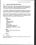 Methods
• Importance of the receiving water area to the surrounding biological
community, e.g., spawning sites, nursery/forage areas, migratory pathways
and areas necessary for critical life stages/functions of an organism;
• The existence of special aquatic sites, including (but not limited to) marine
sanctuaries/refuges, parks, monuments, national seashores, wilderness
areas, coral reefs/seagrass beds;
• Existing or potential recreational and commercial fishing; and
• Any applicable requirements of an approved CZMP.
The identification and delineation of these habitats should be made in both temporal and
spatial dimensions to account for variations in use by the biological community
throughout the year. Both the aerial extent and the functional value to biological
resources must be determined in considering the identification and importance of a
sensitive marine habitat.
Even though an effluent discharge may not directly alter the biological population in a
certain area, if the habitat essential for the survival of those individuals is destroyed, the
ecological results could be the same as if the population had been exposed directly.
The loss of critical habitat could cause the supported population to be either removed or
displaced to less suitable habitat.
Monitoring of discharge effects can help to ensure that long-term sublethal doses do not
accumulate and become toxic. It can also provide assurance that effects such as
increased turbidity or sedimentation do not reduce biological resource productivity below
sustainable levels.
During the permit review process, all important and sensitive habitats should be
identified and delineated to serve as a baseline for future monitoring activities. Habitat
quality in terms of functional values for fish, bird, and marine mammal populations must
also be taken into account to gain a complete valuation of the resources that could be
affected by discharges. Some habitat monitoring activities overlap with other biological
monitoring activities described in other sections. For habitats, the main concern is to
map the physical boundaries and to correlate biological populations to changes in
habitat distributions and functional values.
4.9.2 Monitoring Design Considerations
Habitat monitoring is a two-part process. First, the aerial coverage and boundaries must
be determined; second, the importance or the functional value to biological resources
must be determined. The first determination can be made by using charts, remote
sensing, or submersible remotely operated vehicles. The second analysis is carried out
by using quantification techniques to establish the value of that habitat for particular
166
image:
Methods
• Importance of the receiving water area to the surrounding biological
community, e.g., spawning sites, nursery/forage areas, migratory pathways
and areas necessary for critical life stages/functions of an organism;
• The existence of special aquatic sites, including (but not limited to) marine
sanctuaries/refuges, parks, monuments, national seashores, wilderness
areas, coral reefs/seagrass beds;
• Existing or potential recreational and commercial fishing; and
• Any applicable requirements of an approved CZMP.
The identification and delineation of these habitats should be made in both temporal and
spatial dimensions to account for variations in use by the biological community
throughout the year. Both the aerial extent and the functional value to biological
resources must be determined in considering the identification and importance of a
sensitive marine habitat.
Even though an effluent discharge may not directly alter the biological population in a
certain area, if the habitat essential for the survival of those individuals is destroyed, the
ecological results could be the same as if the population had been exposed directly.
The loss of critical habitat could cause the supported population to be either removed or
displaced to less suitable habitat.
Monitoring of discharge effects can help to ensure that long-term sublethal doses do not
accumulate and become toxic. It can also provide assurance that effects such as
increased turbidity or sedimentation do not reduce biological resource productivity below
sustainable levels.
During the permit review process, all important and sensitive habitats should be
identified and delineated to serve as a baseline for future monitoring activities. Habitat
quality in terms of functional values for fish, bird, and marine mammal populations must
also be taken into account to gain a complete valuation of the resources that could be
affected by discharges. Some habitat monitoring activities overlap with other biological
monitoring activities described in other sections. For habitats, the main concern is to
map the physical boundaries and to correlate biological populations to changes in
habitat distributions and functional values.
4.9.2 Monitoring Design Considerations
Habitat monitoring is a two-part process. First, the aerial coverage and boundaries must
be determined; second, the importance or the functional value to biological resources
must be determined. The first determination can be made by using charts, remote
sensing, or submersible remotely operated vehicles. The second analysis is carried out
by using quantification techniques to establish the value of that habitat for particular
166
image:
 . Section 403 Procedural and Monitoring Quittance
species. The combining of these two techniques allows the identification of those
habitats critical to the functioning of the ecosystem. The determination of the functional
value of a habitat is much more subjective than delineation and must be done with care.
The results of these procedures should be combined with data on trends in species
distribution and water quality to provide a more complete assessment of the causes and
potential effects of habitat degradation. Habitat monitoring will also indicate which
environmental parameters and areas are critical to the ecosystem so that monitoring
activities can be tailored to assess these needs.
To conduct a habitat trend analysis, the sampling design must account for natural
variations caused by extraordinary meteorological events and other phenomena. The
recovery rate of habitat functions and its effects on the functional analysis described
above must also be considered. The primary concern of the habitat assessment is to
accumulate an adequate set of baseline data from which trends can be established.
During this initial phase, seasonal variations must be taken into account during sampling
phases. Sampling and delineation should be carried out at times of maximum biomass
or physical extent. For example, SAV beds or ice floes go through seasonal declines (or
disappearances) and thus a finite period of time exists to conduct sampling. Diurnal
factors such as tides and weather conditions also affect biological populations, and
sampling must be conducted taking these factors into account.
4.9.3 Analytical Methods Considerations
Habitats are generally classified in a hierarchical scheme as mentioned above.
Classification methods that can be used are referenced in Appendix A. The first course
of action in identifying, delineating, and evaluating critical marine habitats entails
mapping out the boundaries of the habitat, while the second involves a determination of
its value as an ecological resource. Table 4-23 lists the methods that can be used to
identify and evaluate sensitive habitats.
Table 4-23. List of Analytical Methods
Areal Trends
Functional Trends
Aerial Photography
Maps
Satellite Imagery
Remotely Operated Vehicles
Habitat Evaluation Procedure (HEP)
Habitat Suitability Modeling
Minimum Habitat Matrix
Wetland Evaluation Technique (WET)
167
image:
. Section 403 Procedural and Monitoring Quittance
species. The combining of these two techniques allows the identification of those
habitats critical to the functioning of the ecosystem. The determination of the functional
value of a habitat is much more subjective than delineation and must be done with care.
The results of these procedures should be combined with data on trends in species
distribution and water quality to provide a more complete assessment of the causes and
potential effects of habitat degradation. Habitat monitoring will also indicate which
environmental parameters and areas are critical to the ecosystem so that monitoring
activities can be tailored to assess these needs.
To conduct a habitat trend analysis, the sampling design must account for natural
variations caused by extraordinary meteorological events and other phenomena. The
recovery rate of habitat functions and its effects on the functional analysis described
above must also be considered. The primary concern of the habitat assessment is to
accumulate an adequate set of baseline data from which trends can be established.
During this initial phase, seasonal variations must be taken into account during sampling
phases. Sampling and delineation should be carried out at times of maximum biomass
or physical extent. For example, SAV beds or ice floes go through seasonal declines (or
disappearances) and thus a finite period of time exists to conduct sampling. Diurnal
factors such as tides and weather conditions also affect biological populations, and
sampling must be conducted taking these factors into account.
4.9.3 Analytical Methods Considerations
Habitats are generally classified in a hierarchical scheme as mentioned above.
Classification methods that can be used are referenced in Appendix A. The first course
of action in identifying, delineating, and evaluating critical marine habitats entails
mapping out the boundaries of the habitat, while the second involves a determination of
its value as an ecological resource. Table 4-23 lists the methods that can be used to
identify and evaluate sensitive habitats.
Table 4-23. List of Analytical Methods
Areal Trends
Functional Trends
Aerial Photography
Maps
Satellite Imagery
Remotely Operated Vehicles
Habitat Evaluation Procedure (HEP)
Habitat Suitability Modeling
Minimum Habitat Matrix
Wetland Evaluation Technique (WET)
167
image:
 Methods
Habitat Delineation
Aerial Photography
Various government agencies (NOAA and USGS among others) have used aircraft to
produce aerial photographs of wide areas for a number of years. The use of
photographs in delineating marine habitats is of limited value since many features below
the low tide line cannot be viewed. Aerial photographs can be produced in a large range
of scales and spatial resolutions depending on the area in question. Fine detail can be
resolved for relatively small tracts, while large areas can be viewed at lower resolutions
to define gross features. In some regions there is an extensive record of historical
photographs that can be used to spot trends and to establish a baseline. New
overflights can be expensive and require ideal weather conditions, but they can be of
value for intertidal mapping and for mapping some submerged aquatic vegetation and
other shallow-water habitats.
Maps
As a preliminary method, maps and charts can be used to obtain a quick assessment of
the presence and delineation of sensitive habitats in the discharge area. Maps are the
least expensive spatial data source and are also the most simple. Nautical charts,
compiled by the Coast and Geodetic Survey of NOAA, contain bottom characteristic
information that could indicate the location of areas of biological importance. This
information is generally accurate for shallow-water areas but may be fragmentary or
nonexistent for areas farther offshore. The coordinated use of U.S. Geological Survey
topographic quadrangle maps, U.S. Fish and Wildlife Service National Wetlands
Inventory maps, and NOAA nautical charts can serve as an information base.
The principal advantages of using maps for delineating habitats is their ease of use and
their low cost. Disadvantages include the inaccuracies in the plotting of habitat
boundaries and the fact that the maps in use may be outdated and thus do not reflect
current conditions. In locations that have a history of human use, there may be an
extensive list of earlier chart or map editions.' These earlier editions can be an excellent
resource for spotting changes in habitat structure.
Satellite Imagery
Satellite imagery is a potential source of data when very large study areas are evaluated
and fine spatial detail is not required. This technique is useful to a maximum depth of
approximately 30 meters, and habitats can be resolved only to a minimum of roughly 30
to 50 square meters. For large study areas, the cost of satellite images can be high,
especially when a long-term temporal series may be required for monitoring purposes.
If the area under investigation contains large homogenous habitats, the resolution size
may not be a constraining factor. A major benefit of these images is that the spectral
168
image:
Methods
Habitat Delineation
Aerial Photography
Various government agencies (NOAA and USGS among others) have used aircraft to
produce aerial photographs of wide areas for a number of years. The use of
photographs in delineating marine habitats is of limited value since many features below
the low tide line cannot be viewed. Aerial photographs can be produced in a large range
of scales and spatial resolutions depending on the area in question. Fine detail can be
resolved for relatively small tracts, while large areas can be viewed at lower resolutions
to define gross features. In some regions there is an extensive record of historical
photographs that can be used to spot trends and to establish a baseline. New
overflights can be expensive and require ideal weather conditions, but they can be of
value for intertidal mapping and for mapping some submerged aquatic vegetation and
other shallow-water habitats.
Maps
As a preliminary method, maps and charts can be used to obtain a quick assessment of
the presence and delineation of sensitive habitats in the discharge area. Maps are the
least expensive spatial data source and are also the most simple. Nautical charts,
compiled by the Coast and Geodetic Survey of NOAA, contain bottom characteristic
information that could indicate the location of areas of biological importance. This
information is generally accurate for shallow-water areas but may be fragmentary or
nonexistent for areas farther offshore. The coordinated use of U.S. Geological Survey
topographic quadrangle maps, U.S. Fish and Wildlife Service National Wetlands
Inventory maps, and NOAA nautical charts can serve as an information base.
The principal advantages of using maps for delineating habitats is their ease of use and
their low cost. Disadvantages include the inaccuracies in the plotting of habitat
boundaries and the fact that the maps in use may be outdated and thus do not reflect
current conditions. In locations that have a history of human use, there may be an
extensive list of earlier chart or map editions.' These earlier editions can be an excellent
resource for spotting changes in habitat structure.
Satellite Imagery
Satellite imagery is a potential source of data when very large study areas are evaluated
and fine spatial detail is not required. This technique is useful to a maximum depth of
approximately 30 meters, and habitats can be resolved only to a minimum of roughly 30
to 50 square meters. For large study areas, the cost of satellite images can be high,
especially when a long-term temporal series may be required for monitoring purposes.
If the area under investigation contains large homogenous habitats, the resolution size
may not be a constraining factor. A major benefit of these images is that the spectral
168
image:
 Section 403 Procedural and Monitoring Guidance
properties and brightness values are recorded digitally. This technology lends itself to
advanced spatial analysis methods that can be used to quantify productivity values.
These determinations are not possible with most aerial photographs.
Remotely Operated Vehicles
Remotely operated vehicles (ROVs) are small, unmanned, remotely operated
submersibles that are equipped with lights and cameras used to view portions of the
ocean bottom. These submersibles receive power and commands from a support
vessel and are highly versatile for identifying possible habitats. EPA Region 4 has used
ROVs to investigate and record the ocean bottom immediately'surrounding the
discharge outfalls of oil and gas drilling wells. This methodology produces a precise,
nondestructive record of the nature and extent of any physical habitat. The main liability
of this system is that unless vast amounts of time are spent, only small areas can be
investigated. These systems are also rather expensive and require well-trained
technicians to operate them. In addition, a ROV is limited by the length of its umbilical
and by the visibility of the water column in the search area. The visibility problem may
be compensated for by the addition of such technology as side scan sonar or sonar
attached to the ROV. Because of these constraints, the use of this system would be
confined to areas of most concern near the zone of initial dilution.
Functional Analysis
Functional analysis attempts to assess the use of the habitat by biological resources and
to compare the value of one habitat to that of another. Another aspect of functional
analysis is to calculate the change in a habitat's value over time. These processes
entail site-specific studies that can involve a large amount of time and money. The data
required by this technique can be collected in connection with the techniques described
in the biological methods section of this report. The analysis of these data will center on
spatial and temporal variations at a particular habitat. Various methods for conducting
functional analysis are referenced in Appendix A. Some of the most widely used
procedures are described below.
Habitat Evaluation Procedures
Habitat evaluation procedures (HEPs) are procedures developed by the U. S. Fish and
Wildlife Service to document the quality and quantity of available habitat for selected
wildlife species. The data generated are used to compare two habitats at the same
point in time and a single habitat over a length of time. By combining these two sets of
information, the impact of proposed discharges can be quantified (Lonard and Clairain,
1986).
169
image:
Section 403 Procedural and Monitoring Guidance
properties and brightness values are recorded digitally. This technology lends itself to
advanced spatial analysis methods that can be used to quantify productivity values.
These determinations are not possible with most aerial photographs.
Remotely Operated Vehicles
Remotely operated vehicles (ROVs) are small, unmanned, remotely operated
submersibles that are equipped with lights and cameras used to view portions of the
ocean bottom. These submersibles receive power and commands from a support
vessel and are highly versatile for identifying possible habitats. EPA Region 4 has used
ROVs to investigate and record the ocean bottom immediately'surrounding the
discharge outfalls of oil and gas drilling wells. This methodology produces a precise,
nondestructive record of the nature and extent of any physical habitat. The main liability
of this system is that unless vast amounts of time are spent, only small areas can be
investigated. These systems are also rather expensive and require well-trained
technicians to operate them. In addition, a ROV is limited by the length of its umbilical
and by the visibility of the water column in the search area. The visibility problem may
be compensated for by the addition of such technology as side scan sonar or sonar
attached to the ROV. Because of these constraints, the use of this system would be
confined to areas of most concern near the zone of initial dilution.
Functional Analysis
Functional analysis attempts to assess the use of the habitat by biological resources and
to compare the value of one habitat to that of another. Another aspect of functional
analysis is to calculate the change in a habitat's value over time. These processes
entail site-specific studies that can involve a large amount of time and money. The data
required by this technique can be collected in connection with the techniques described
in the biological methods section of this report. The analysis of these data will center on
spatial and temporal variations at a particular habitat. Various methods for conducting
functional analysis are referenced in Appendix A. Some of the most widely used
procedures are described below.
Habitat Evaluation Procedures
Habitat evaluation procedures (HEPs) are procedures developed by the U. S. Fish and
Wildlife Service to document the quality and quantity of available habitat for selected
wildlife species. The data generated are used to compare two habitats at the same
point in time and a single habitat over a length of time. By combining these two sets of
information, the impact of proposed discharges can be quantified (Lonard and Clairain,
1986).
169
image:
 Methods
In the evaluation procedure, the habitat quality of selected species is documented based
on an evaluation of the ability of key habitat components to supply the life requisites of
the selected species. The evaluation involves using the same key habitat components
to compare existing habitat conditions and the optimum conditions for the species of
interest (USFWS, 1980).
The limitations in using this approach involve the use of habitat quality as an evaluation
parameter, which limits the methodology to those situations in which measurable and
predictable habitat changes are an important variable. This approach also forces a
long-term averaging type of analysis. There is no assurance that populations will exist
at the levels predicted by the analysis since all the environmental or behavior variables
that affect population levels may not be included. In addition, socioeconomic or political
constraints not taken into account may prevent the actual populations from reaching
their predicted levels (USFWS, 1980).
Habitat Suitability Modeling
Habitat suitability modeling consolidates habitat use information into a framework
appropriate for field application and is scaled to produce an index between 0.0 (unsuitable
habitat) and 1.0 (optimum habitat). Habitat suitability models are designed for use with the
habitat evaluation procedures described above (Toole et al., 1987). Multiple regression
equations are used to describe relationships between environmental characteristics and
productivity. Once the model has been validated, sensitivity analysis can be carried out to
project the results of varied discharge rates on the health of the site.
For modeling to make reliable predications, the input data must accurately reflect the
range of natural conditions observed. This may involve expensive and time-consuming
field studies in which the error limits and the QA/QC parameters must be well defined.
The reliability and the extent of the field data can be a major limitation in these studies.
Minimum Habitat Matrix
Minimum habitat guidelines for various species are a technique developed with the
ultimate goal of reestablishing balanced ecosystems in environmentally stressed areas.
This method is designed to provide information on the minimum habitat quality needed
by a target species and identifies those factors (both environmental and ecological)
required for the species. This information is formatted into a habitat requirement matrix
that defines the habitat parameters needed for successful reproduction and survival of
the indicated species. Such matrices can indicate the vital environmental parameters
that should be monitored, thus facilitating the development of monitoring programs. This
process is used to estimate the feasibility, benefits, and potential costs of maintaining
and protecting an estuarine environment suitable for the successful reproduction and
survival of the indicated species (Chesapeake Executive Council, 1988a).
170
image:
Methods
In the evaluation procedure, the habitat quality of selected species is documented based
on an evaluation of the ability of key habitat components to supply the life requisites of
the selected species. The evaluation involves using the same key habitat components
to compare existing habitat conditions and the optimum conditions for the species of
interest (USFWS, 1980).
The limitations in using this approach involve the use of habitat quality as an evaluation
parameter, which limits the methodology to those situations in which measurable and
predictable habitat changes are an important variable. This approach also forces a
long-term averaging type of analysis. There is no assurance that populations will exist
at the levels predicted by the analysis since all the environmental or behavior variables
that affect population levels may not be included. In addition, socioeconomic or political
constraints not taken into account may prevent the actual populations from reaching
their predicted levels (USFWS, 1980).
Habitat Suitability Modeling
Habitat suitability modeling consolidates habitat use information into a framework
appropriate for field application and is scaled to produce an index between 0.0 (unsuitable
habitat) and 1.0 (optimum habitat). Habitat suitability models are designed for use with the
habitat evaluation procedures described above (Toole et al., 1987). Multiple regression
equations are used to describe relationships between environmental characteristics and
productivity. Once the model has been validated, sensitivity analysis can be carried out to
project the results of varied discharge rates on the health of the site.
For modeling to make reliable predications, the input data must accurately reflect the
range of natural conditions observed. This may involve expensive and time-consuming
field studies in which the error limits and the QA/QC parameters must be well defined.
The reliability and the extent of the field data can be a major limitation in these studies.
Minimum Habitat Matrix
Minimum habitat guidelines for various species are a technique developed with the
ultimate goal of reestablishing balanced ecosystems in environmentally stressed areas.
This method is designed to provide information on the minimum habitat quality needed
by a target species and identifies those factors (both environmental and ecological)
required for the species. This information is formatted into a habitat requirement matrix
that defines the habitat parameters needed for successful reproduction and survival of
the indicated species. Such matrices can indicate the vital environmental parameters
that should be monitored, thus facilitating the development of monitoring programs. This
process is used to estimate the feasibility, benefits, and potential costs of maintaining
and protecting an estuarine environment suitable for the successful reproduction and
survival of the indicated species (Chesapeake Executive Council, 1988a).
170
image:
 Section 403 Procedural and Monitoring Guidance
One potential problem with this method is that the primary indicated species and those
organisms on which the target species depend for food are both tracked with the
intention of maintaining habitat quality for both. This method may not completely
recognize the complex species interdependence within marine environments.
Wetland Evaluation Technique
The wetland evaluation technique (WET) was initially developed by the Federal Highway
Administration and revised by the U.S. Army Corps of Engineers to assess the function
and value of various components of habitats and their suitability for specific fish and
invertebrate species. WET evaluates functions and values in terms of social
significance, effectiveness, and opportunity (Adamus et al., 1987). Social significance
assesses the value of a site to society due to its special designation, potential economic
value, and strategic location. Effectiveness assesses the capability of a wetland to
perform a function as a result of its physical, chemical, or biological characteristics.
Opportunity assesses the opportunity for a habitat to perform a function to its level of
capability.
WET assesses functions and values by characterizing a habitat in terms of its physical,
chemical, and biological processes and attributes (Adamus et al., 1987). This
characterization is accomplished by identifying threshold values for predictors.
Predictors are simple, or integrated, variables that directly or indirectly measure the
physical, chemical, and biological processes or attributes of a habitat and its
surroundings.
4.9.4 QA/QC Considerations
Since sensitive habitat identification is relatively subjective, close controls must be
exercised during sampling and delineation. In the delineation of habitats, two individuals
should independently define the boundaries of a single habitat area. Any disagreement
between the two should be rectified before a final determination is reached. Sampling
programs demand a high level of expertise on the part of the individuals conducting
them. All personnel must have an advanced understanding of such topics as taxonomy,
sampling techniques, and statistics. The sampling strategy used will depend at least in
part on the level of expertise or training available. The selection of a functional analysis
method should be made after a review of the strengths and limitations of each method
has been conducted.
4.9.5 Statistical Design Considerations
In designing a habitat monitoring program, the researcher must first determine the
resources available. This will determine the extent of the monitoring program and the
level of detail it can provide. Aerial assessment can be done with limited resources,
while functional analysis requires greater commitments of both finances and time.
171
image:
Section 403 Procedural and Monitoring Guidance
One potential problem with this method is that the primary indicated species and those
organisms on which the target species depend for food are both tracked with the
intention of maintaining habitat quality for both. This method may not completely
recognize the complex species interdependence within marine environments.
Wetland Evaluation Technique
The wetland evaluation technique (WET) was initially developed by the Federal Highway
Administration and revised by the U.S. Army Corps of Engineers to assess the function
and value of various components of habitats and their suitability for specific fish and
invertebrate species. WET evaluates functions and values in terms of social
significance, effectiveness, and opportunity (Adamus et al., 1987). Social significance
assesses the value of a site to society due to its special designation, potential economic
value, and strategic location. Effectiveness assesses the capability of a wetland to
perform a function as a result of its physical, chemical, or biological characteristics.
Opportunity assesses the opportunity for a habitat to perform a function to its level of
capability.
WET assesses functions and values by characterizing a habitat in terms of its physical,
chemical, and biological processes and attributes (Adamus et al., 1987). This
characterization is accomplished by identifying threshold values for predictors.
Predictors are simple, or integrated, variables that directly or indirectly measure the
physical, chemical, and biological processes or attributes of a habitat and its
surroundings.
4.9.4 QA/QC Considerations
Since sensitive habitat identification is relatively subjective, close controls must be
exercised during sampling and delineation. In the delineation of habitats, two individuals
should independently define the boundaries of a single habitat area. Any disagreement
between the two should be rectified before a final determination is reached. Sampling
programs demand a high level of expertise on the part of the individuals conducting
them. All personnel must have an advanced understanding of such topics as taxonomy,
sampling techniques, and statistics. The sampling strategy used will depend at least in
part on the level of expertise or training available. The selection of a functional analysis
method should be made after a review of the strengths and limitations of each method
has been conducted.
4.9.5 Statistical Design Considerations
In designing a habitat monitoring program, the researcher must first determine the
resources available. This will determine the extent of the monitoring program and the
level of detail it can provide. Aerial assessment can be done with limited resources,
while functional analysis requires greater commitments of both finances and time.
171
image:
 Methods
Functional assessments require that the researcher decide which functions are of
greatest interest in the area of study or which will provide the most information
concerning the habitat attributes perceived to be of greatest value to the area.
Most habitat evaluation techniques involve some form of ranking, either quantitative or
qualitative. The purpose of the monitoring program is to periodically compare baseline
conditions to conditions after the permit has been issued. In terms of habitat monitoring,
this means comparing the baseline acreage or functional rating of the habitat to
conditions some time after discharge has commenced. Therefore, the ability to replicate
results is imperative.
4.9.6 Use of Data
The object of the data set is to obtain a clear and precise spatial and temporal picture of
the physical extent of a sensitive habitat. An evaluation of the functional value of that
habitat is also made so that the effects of various impacts can be judged. Sensitive
habitats should be clearly delineated on nautical charts or topographic maps along with
a complete description of their composition. The description should include a
characterization of the extent of natural seasonal variations in the boundaries. A
complete description of the functional value of the habitat to the biological community,
as well as an estimate of potential for loss of the resource from the effects of effluent
discharge, should also be made.
These data will act as a baseline for future monitoring programs that will track the
changes to the system. The baseline study and the monitoring program should be able
to discriminate between natural variations and discharge-induced changes.
4.9.7 Summary and Recommendations
Rationale
A sensitive habitat can be defined as a physical area utilized, at least for a
significant portion of the year, by a disproportionate abundance of individuals
and/or species, or as an area essential to the functioning of the ecosystem.
Sensitive marine habitats should be identified and their boundaries delineated
as part of an ongoing effort to assess the potential for impacts from effluent
discharges on ecological communities.
Monitoring programs that assess both the physical boundaries of the habitats
and the support functions that they serve for biological communities should
be conducted when sensitive habitats are present.
Damage to habitats from discharge effluents can cause irreversible harm and
create severe changes in ecosystem function and diversity.
172
image:
Methods
Functional assessments require that the researcher decide which functions are of
greatest interest in the area of study or which will provide the most information
concerning the habitat attributes perceived to be of greatest value to the area.
Most habitat evaluation techniques involve some form of ranking, either quantitative or
qualitative. The purpose of the monitoring program is to periodically compare baseline
conditions to conditions after the permit has been issued. In terms of habitat monitoring,
this means comparing the baseline acreage or functional rating of the habitat to
conditions some time after discharge has commenced. Therefore, the ability to replicate
results is imperative.
4.9.6 Use of Data
The object of the data set is to obtain a clear and precise spatial and temporal picture of
the physical extent of a sensitive habitat. An evaluation of the functional value of that
habitat is also made so that the effects of various impacts can be judged. Sensitive
habitats should be clearly delineated on nautical charts or topographic maps along with
a complete description of their composition. The description should include a
characterization of the extent of natural seasonal variations in the boundaries. A
complete description of the functional value of the habitat to the biological community,
as well as an estimate of potential for loss of the resource from the effects of effluent
discharge, should also be made.
These data will act as a baseline for future monitoring programs that will track the
changes to the system. The baseline study and the monitoring program should be able
to discriminate between natural variations and discharge-induced changes.
4.9.7 Summary and Recommendations
Rationale
A sensitive habitat can be defined as a physical area utilized, at least for a
significant portion of the year, by a disproportionate abundance of individuals
and/or species, or as an area essential to the functioning of the ecosystem.
Sensitive marine habitats should be identified and their boundaries delineated
as part of an ongoing effort to assess the potential for impacts from effluent
discharges on ecological communities.
Monitoring programs that assess both the physical boundaries of the habitats
and the support functions that they serve for biological communities should
be conducted when sensitive habitats are present.
Damage to habitats from discharge effluents can cause irreversible harm and
create severe changes in ecosystem function and diversity.
172
image:
 Section 403 Procedural and Monitoring Guidance
• Monitoring programs can provide assurance that effects such as increased
turbidity or sedimentation do not reduce biological resource productivity
below sustainable levels.
Monitoring Design Considerations
• Habitat monitoring consists of two parts: (1) aerial coverage and boundary
delineation and (2) functional analysis, which determines the value of the
habitat to the system.
• Habitat delineation can be fairly straightforward, but functional analysis is
rather subjective and must be done with care.
• Sampling strategies must account for variations caused by natural processes
and must be done at times of maximum extent or biomass.
• A functional analysis technique should be selected after a review of the
strengths and limitations of each method for each particular site.
Analytical Methods Considerations
• Sensitive habitats can be identified using maps, charts, and photographic
techniques. ROVs can be used to investigate near-field habitats in the zone
of initial dilution.
• Functional analysis determines the importance of a habitat to the biological
community.
• Functional analysis techniques are based on theoretical relationships of the
ecosystem; consequently, both the theory and the data used should be
vigorously evaluated.
• For habitat identification and delineations, the following techniques can be
used:
- aerial photography,
- maps/charts,
- satellite imagery, and
- remotely operated vehicles.
• Functional analysis can be carried out using various methods. Those
described are the following:
- habitat evaluation procedures (HEP),
- wetland evaluation technique (WET),
- habitat suitability modeling, and
- minimum habitat matrix.
773
image:
Section 403 Procedural and Monitoring Guidance
• Monitoring programs can provide assurance that effects such as increased
turbidity or sedimentation do not reduce biological resource productivity
below sustainable levels.
Monitoring Design Considerations
• Habitat monitoring consists of two parts: (1) aerial coverage and boundary
delineation and (2) functional analysis, which determines the value of the
habitat to the system.
• Habitat delineation can be fairly straightforward, but functional analysis is
rather subjective and must be done with care.
• Sampling strategies must account for variations caused by natural processes
and must be done at times of maximum extent or biomass.
• A functional analysis technique should be selected after a review of the
strengths and limitations of each method for each particular site.
Analytical Methods Considerations
• Sensitive habitats can be identified using maps, charts, and photographic
techniques. ROVs can be used to investigate near-field habitats in the zone
of initial dilution.
• Functional analysis determines the importance of a habitat to the biological
community.
• Functional analysis techniques are based on theoretical relationships of the
ecosystem; consequently, both the theory and the data used should be
vigorously evaluated.
• For habitat identification and delineations, the following techniques can be
used:
- aerial photography,
- maps/charts,
- satellite imagery, and
- remotely operated vehicles.
• Functional analysis can be carried out using various methods. Those
described are the following:
- habitat evaluation procedures (HEP),
- wetland evaluation technique (WET),
- habitat suitability modeling, and
- minimum habitat matrix.
773
image:
 Methods
QA/QC Considerations
• Personnel identifying habitat should have advanced training, and two people
should independently define the boundaries.
Study Design Considerations
• Ability to replicate results is important.
• The extent of the monitoring program can be based on funding level.
• Aerial assessments are inexpensive, while functional analyses are more
expensive and more labor-intensive.
Use of Data
• Data collected will consist of charts identifying the boundaries of sensitive
habitats accompanied by complete descriptions.
• Functional analysis results will indicate which habitats are critical and the
effects observed under various discharge scenarios.
174
image:
Methods
QA/QC Considerations
• Personnel identifying habitat should have advanced training, and two people
should independently define the boundaries.
Study Design Considerations
• Ability to replicate results is important.
• The extent of the monitoring program can be based on funding level.
• Aerial assessments are inexpensive, while functional analyses are more
expensive and more labor-intensive.
Use of Data
• Data collected will consist of charts identifying the boundaries of sensitive
habitats accompanied by complete descriptions.
• Functional analysis results will indicate which habitats are critical and the
effects observed under various discharge scenarios.
174
image:
 Section 403 Procedural and Monitoring Guidance
4.10 BIOACCUMULATION
Bioaccumulation is the overall process of biological uptake and retention of chemical
contaminants obtained from foods, water, sediments, or any combination of exposure
pathways. A number of expressions are used to describe the bioaccumulation potential
of contaminants. These terms are explained in Table 4-24. Bioaccumulation is a
consequence of an organism's physiological limitations to transform and excrete the
invading chemical substances. Potential consequences of bioaccumulation of chemical
contaminants in marine organisms include, but are not limited to:
• Significant mortality to susceptible organisms;
• Lethal or sublethal chronic toxic responses at later stages of the life cycle or
under conditions of stress for susceptible organisms; and
• Transference of increasingly greater concentrations of toxic pollutants to
organisms at higher trophic levels, including humans.
Bioaccumulation analyses provide the link between exposure and effects and thus can
generate important insights into ecological effects, human health risks, and routes and
extent of pollutant exposure.
4.10.1 Rationale
The Clean Water Act section 403 point source discharge program requires (among other
things) a determination of:
Bioavailability
Bioaccumulation
Bioconcentration
Biomagnification
Table 4-24. List of Terms
A measure of the physicochemical access that a toxicant has to the
biological processes of an organism. The less the bioavailability of a
toxicant, the less its toxic effect on an organism (USEPA, 1991c).
Uptake and retention of substances by an organism from its surrounding
medium and from food (USEPA, 1990a).
Uptake of substances by an organism from the surrounding medium through
gill membranes or other external body surfaces (USEPA, 1990a).
The process by which the concentration of a compound increases in different
organisms occupying successive trophic levels (USEPA, 1990a)
175
image:
Section 403 Procedural and Monitoring Guidance
4.10 BIOACCUMULATION
Bioaccumulation is the overall process of biological uptake and retention of chemical
contaminants obtained from foods, water, sediments, or any combination of exposure
pathways. A number of expressions are used to describe the bioaccumulation potential
of contaminants. These terms are explained in Table 4-24. Bioaccumulation is a
consequence of an organism's physiological limitations to transform and excrete the
invading chemical substances. Potential consequences of bioaccumulation of chemical
contaminants in marine organisms include, but are not limited to:
• Significant mortality to susceptible organisms;
• Lethal or sublethal chronic toxic responses at later stages of the life cycle or
under conditions of stress for susceptible organisms; and
• Transference of increasingly greater concentrations of toxic pollutants to
organisms at higher trophic levels, including humans.
Bioaccumulation analyses provide the link between exposure and effects and thus can
generate important insights into ecological effects, human health risks, and routes and
extent of pollutant exposure.
4.10.1 Rationale
The Clean Water Act section 403 point source discharge program requires (among other
things) a determination of:
Bioavailability
Bioaccumulation
Bioconcentration
Biomagnification
Table 4-24. List of Terms
A measure of the physicochemical access that a toxicant has to the
biological processes of an organism. The less the bioavailability of a
toxicant, the less its toxic effect on an organism (USEPA, 1991c).
Uptake and retention of substances by an organism from its surrounding
medium and from food (USEPA, 1990a).
Uptake of substances by an organism from the surrounding medium through
gill membranes or other external body surfaces (USEPA, 1990a).
The process by which the concentration of a compound increases in different
organisms occupying successive trophic levels (USEPA, 1990a)
175
image:
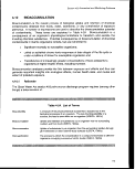 Methods
• The quantities, composition, and potential for bioaccumulation or persistence
of the pollutants to be discharged;
• The potential transport of the pollutants by biological, physical, or chemical
processes;
• The composition and vulnerability of potentially exposed biological communities;
and
• Potential direct or indirect impacts on human health.
Each of these determinations is addressed to some degree through bioaccumulation
studies.
Monitoring of bioaccumulation data is essential in relating the presence of selected
chemical residues in marine waters and sediment to their transfer and accumulation in
marine organisms and potential transfer to humans. Toxics can occur in the water
column at or near analytical detection limits; however, over time, these contaminants
can accumulate in fish and shellfish tissue to measurable concentrations. In areas
where water and sediments show measurable contaminant levels, it is difficult at best to
predict rates of uptake and bioaccumulation, although direct monitoring can provide
spatial and temporal records of the concentration and bioaccumulation of toxics. The
assessment of bioaccumulation in the surrounding biological community should be a
component of a monitoring program required in a permit issued under the "no
irreparable harm" clause of section 403.
4.10.2 Monitoring Design Considerations
Typically, bioaccumulation studies are formulated according to the study objectives. If
the objective is to determine the effects of bioaccumulation on human health, then
commercial and/or recreational fish and shellfish are tested. If determining the effects
on the habitat or ecosystem is the objective, usually the benthic macroinvertebrates are
surveyed. Unfortunately, comparisons between studies are valid only if the study
designs and procedures are comparable. Standardization of monitoring design would
allow for comparison between various studies.
A common deficiency in many programs is the inability to collect sufficient tissue
biomass of appropriate species across sampling locations throughout the study. The
selection of appropriate species and tissues must account for natural fluctuations in
populations as well as changes due to anthropogenic perturbations. Indigenous species
initially present may not be available later, limiting temporal and spatial comparisons.
176
image:
Methods
• The quantities, composition, and potential for bioaccumulation or persistence
of the pollutants to be discharged;
• The potential transport of the pollutants by biological, physical, or chemical
processes;
• The composition and vulnerability of potentially exposed biological communities;
and
• Potential direct or indirect impacts on human health.
Each of these determinations is addressed to some degree through bioaccumulation
studies.
Monitoring of bioaccumulation data is essential in relating the presence of selected
chemical residues in marine waters and sediment to their transfer and accumulation in
marine organisms and potential transfer to humans. Toxics can occur in the water
column at or near analytical detection limits; however, over time, these contaminants
can accumulate in fish and shellfish tissue to measurable concentrations. In areas
where water and sediments show measurable contaminant levels, it is difficult at best to
predict rates of uptake and bioaccumulation, although direct monitoring can provide
spatial and temporal records of the concentration and bioaccumulation of toxics. The
assessment of bioaccumulation in the surrounding biological community should be a
component of a monitoring program required in a permit issued under the "no
irreparable harm" clause of section 403.
4.10.2 Monitoring Design Considerations
Typically, bioaccumulation studies are formulated according to the study objectives. If
the objective is to determine the effects of bioaccumulation on human health, then
commercial and/or recreational fish and shellfish are tested. If determining the effects
on the habitat or ecosystem is the objective, usually the benthic macroinvertebrates are
surveyed. Unfortunately, comparisons between studies are valid only if the study
designs and procedures are comparable. Standardization of monitoring design would
allow for comparison between various studies.
A common deficiency in many programs is the inability to collect sufficient tissue
biomass of appropriate species across sampling locations throughout the study. The
selection of appropriate species and tissues must account for natural fluctuations in
populations as well as changes due to anthropogenic perturbations. Indigenous species
initially present may not be available later, limiting temporal and spatial comparisons.
176
image:
 Section 403 Procedural and Monitoring Quittance
Selection of Target Species
A key component of any bioaccumulation monitoring program is the selection of target
species. Concentrations of chemical residues in tissues of target species serve as
indicators of contamination throughout the biological system. The fundamental criterion
is the ability to use the selected species to make comparisons between sampling
locations and sampling periods.
Target Species Characteristics
It is recommended that the target species possess the following characteristics (USEPA,
1985a):
• High bioaccumulation potential for selected contaminants of concern;
• Weakness or absence of metabolic regulation of selected contaminants to
allow assessment of a "worst-case scenario";
• Abundant enough, temporally and spatially, to allow for adequate sampling;
• Large enough to provide adequate amounts of tissue for analysis;
• Sessile or sedentary in nature to ensure that bioaccumulation is
representative of the study area;
• Easily collected; and
• Part of an existing data base of exposures and sensitivity.
Suggested fish and macroinvertebrate target species for various regions of the United
States are listed in Tables 4-25 and 4-26 (USEPA, 1985a).
Secondary considerations based on economic importance and status as a bioassay
organism may be applied to further winnow the list of candidate target species to a
practical number of species to be analyzed.
Candidate target species should be objectively ranked based on ecological
characteristics that would enhance their potential for bioaccumulation and facilitate
sampling and analytical procedures (USEPA, 1985a). The advantages of using benthic
macroinvertebrates as target species are:
• They are sendentary and therefore represent bioaccumulation in the study
area.
• They represent a significant food source for higher trophic levels and
therefore indicate the existence of contaminants in the food web.
177
image:
Section 403 Procedural and Monitoring Quittance
Selection of Target Species
A key component of any bioaccumulation monitoring program is the selection of target
species. Concentrations of chemical residues in tissues of target species serve as
indicators of contamination throughout the biological system. The fundamental criterion
is the ability to use the selected species to make comparisons between sampling
locations and sampling periods.
Target Species Characteristics
It is recommended that the target species possess the following characteristics (USEPA,
1985a):
• High bioaccumulation potential for selected contaminants of concern;
• Weakness or absence of metabolic regulation of selected contaminants to
allow assessment of a "worst-case scenario";
• Abundant enough, temporally and spatially, to allow for adequate sampling;
• Large enough to provide adequate amounts of tissue for analysis;
• Sessile or sedentary in nature to ensure that bioaccumulation is
representative of the study area;
• Easily collected; and
• Part of an existing data base of exposures and sensitivity.
Suggested fish and macroinvertebrate target species for various regions of the United
States are listed in Tables 4-25 and 4-26 (USEPA, 1985a).
Secondary considerations based on economic importance and status as a bioassay
organism may be applied to further winnow the list of candidate target species to a
practical number of species to be analyzed.
Candidate target species should be objectively ranked based on ecological
characteristics that would enhance their potential for bioaccumulation and facilitate
sampling and analytical procedures (USEPA, 1985a). The advantages of using benthic
macroinvertebrates as target species are:
• They are sendentary and therefore represent bioaccumulation in the study
area.
• They represent a significant food source for higher trophic levels and
therefore indicate the existence of contaminants in the food web.
177
image:
 Methods
B
Table 4-25. Highest-Ranking Candidate Fish for Use
as Bioaccumulation Monitoring Species
Secondary Selection Criteria
State
MASSACHUSETTS
RHODE ISLAND
NEW YORK
NEW JERSEY
VIRGINIA
lE.iir' ^rjaSssi
Locality
Swampscott
Lynn
South Essex
Boston
Fall River
New Bedford
Newport
Upper East River
Lower East River
Lower Hudson River
Cape May
Portsmouth
Virginia Beach
1
Species
Winter flounder
Yellowtail flounder
Ocean pout
Windowpane
Winter flounder
Yellowtail flounder
Ocean pout
Winter flounder
Yellowtail flounder
Windowpane
American eel
Ocean pout
Winter flounder
Yellowtail flounder
Ocean pout
Windowpane
Winter flounder
Windowpane
Winter flounder
Scup
Summer flounder
Winter flounder
Scup
Weakfish
Winter flounder
Windowpane
Weakfish
Spot
Scup
American eel
Hogchoker
Spot
Red hake
Windowpane
Summer flounder
Spot
Summer flounder
Atlantic croaker
Hogchoker
Spot
Red hake
Summer flounder
tea *Jy,'XS >£«""!'»''*••* W»x A
eSst&'r XX^^X' .X •.'•£<^«*^'. "y«"*<iWfiS
Economic
Importance
Yes
Yes
No
No
Yes
Yes
No
Yes
No
No
No
No
Yes
Yes
No
No
Yes
No
Yes
No
Yes
Yes
Yes
Yes
Yes
No
Yes
Yes
Yes
No
No
Yes
No
No
Yes
Yes
Yes
No
No
Yes
No
Yes
* , #*v"*< £$•/£>>>* < < SoftiSw&jjy*'-??'?* ,
Bioassay
Species
Yes
Yes
No
No
Yes
No
No
Yes
No
No
No
No
Yes
No
No
No
Yes
No
Yes
No
Yes
Yes
No
No
Yes
No
No
Yes
No
No
No
Yes
No
No
Yes
Yes
Yes
No
No
Yes
No
Yes
yfAsffiW t.-s'^W-v?*' -. '-., ,v ,-W,
Xi * v'r-v *'""&?£%&*.??£?*
178
image:
Methods
B
Table 4-25. Highest-Ranking Candidate Fish for Use
as Bioaccumulation Monitoring Species
Secondary Selection Criteria
State
MASSACHUSETTS
RHODE ISLAND
NEW YORK
NEW JERSEY
VIRGINIA
lE.iir' ^rjaSssi
Locality
Swampscott
Lynn
South Essex
Boston
Fall River
New Bedford
Newport
Upper East River
Lower East River
Lower Hudson River
Cape May
Portsmouth
Virginia Beach
1
Species
Winter flounder
Yellowtail flounder
Ocean pout
Windowpane
Winter flounder
Yellowtail flounder
Ocean pout
Winter flounder
Yellowtail flounder
Windowpane
American eel
Ocean pout
Winter flounder
Yellowtail flounder
Ocean pout
Windowpane
Winter flounder
Windowpane
Winter flounder
Scup
Summer flounder
Winter flounder
Scup
Weakfish
Winter flounder
Windowpane
Weakfish
Spot
Scup
American eel
Hogchoker
Spot
Red hake
Windowpane
Summer flounder
Spot
Summer flounder
Atlantic croaker
Hogchoker
Spot
Red hake
Summer flounder
tea *Jy,'XS >£«""!'»''*••* W»x A
eSst&'r XX^^X' .X •.'•£<^«*^'. "y«"*<iWfiS
Economic
Importance
Yes
Yes
No
No
Yes
Yes
No
Yes
No
No
No
No
Yes
Yes
No
No
Yes
No
Yes
No
Yes
Yes
Yes
Yes
Yes
No
Yes
Yes
Yes
No
No
Yes
No
No
Yes
Yes
Yes
No
No
Yes
No
Yes
* , #*v"*< £$•/£>>>* < < SoftiSw&jjy*'-??'?* ,
Bioassay
Species
Yes
Yes
No
No
Yes
No
No
Yes
No
No
No
No
Yes
No
No
No
Yes
No
Yes
No
Yes
Yes
No
No
Yes
No
No
Yes
No
No
No
Yes
No
No
Yes
Yes
Yes
No
No
Yes
No
Yes
yfAsffiW t.-s'^W-v?*' -. '-., ,v ,-W,
Xi * v'r-v *'""&?£%&*.??£?*
178
image:
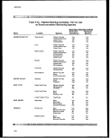 Section 403 Procedural and Monitoring Quittance
* s , ->-.-•/>*•: ^"fj, ',-w, ''3&'j;?3&!
State
CALIFORNIA
(Northern)
CALIFORNIA
(Southern)
WASHINGTON
(^'•^tff^ff, , %J1 ^J'jJ^"** -fr"" V'*'*' **X %'"'****'• > JVJ , V^-Jifc, ^^^^K.^VX'-SSvMX.Xvs^A^'v^v..
' > *% A^V •." ' ' ' ' ^"'-s i /' * rti ' ,* Vv * •>•*«''* ^»i?v ^ - •• ^-V"V " ' * V»t"A' o' 5 > * >£ b^pw- v;
Table 4-25. (continued)
Locality
San Francisco
Oakland
Monterey
Santa Cruz
Watsonville
Goleta
Santa Barbara
L.A. County
Orange County
Hyperion
Oceanside
Escondido
San Elijo
San Diego
Central Puget Sound
^fy^ t°'Vv- •",, "
Secondary Selection Criteria
Economic Bioassay
Species Importance Species
English sole
Pacific sanddab
Big skate
English sole
Starry flounder
Pacific staghorn
sculpin
English sole
Curlfin sole
English sole
English sole
Curlfin sole
Dover sole
Pacific sanddab
Longspine combfish
Spotted cusk-eel
English sole
Pacific sanddab
Dover sole
Curlfin sole
English sole
Dover sole
Pacific sanddab
English sole
Dover sole
Longspine combfish
Big skate
California skate
Dover sole
Blackbelly eelpout
Pacific sanddab
English sole
Dover sole
English sole
Pacific sanddab
Longspine combfish
English sole
Dover sole
Rock sole
Spotted ratfish
Rex sole
C-O sole
Yes
Yes
No
Yes
Yes
No
Yes
Yes
Yes
Yes
Yes
Yes
Yes
No
No
Yes
Yes
No
No
Yes
Yes
Yes
Yes
Yes
No
No
No
Yes
No
Yes
Yes
Yes
Yes
Yes
No
Yes
Yes
Yes
No
Yes
Yes
Yes
No
No
Yes
No
No
Yes
No
Yes
Yes
No
No
No
No
No
Yes
No
No
No
Yes
Yes
Yes
Yes
No
No
No
No
No
No
No
Yes
No
Yes
No
No
Yes
No
No
No
No
No
179
image:
Section 403 Procedural and Monitoring Quittance
* s , ->-.-•/>*•: ^"fj, ',-w, ''3&'j;?3&!
State
CALIFORNIA
(Northern)
CALIFORNIA
(Southern)
WASHINGTON
(^'•^tff^ff, , %J1 ^J'jJ^"** -fr"" V'*'*' **X %'"'****'• > JVJ , V^-Jifc, ^^^^K.^VX'-SSvMX.Xvs^A^'v^v..
' > *% A^V •." ' ' ' ' ^"'-s i /' * rti ' ,* Vv * •>•*«''* ^»i?v ^ - •• ^-V"V " ' * V»t"A' o' 5 > * >£ b^pw- v;
Table 4-25. (continued)
Locality
San Francisco
Oakland
Monterey
Santa Cruz
Watsonville
Goleta
Santa Barbara
L.A. County
Orange County
Hyperion
Oceanside
Escondido
San Elijo
San Diego
Central Puget Sound
^fy^ t°'Vv- •",, "
Secondary Selection Criteria
Economic Bioassay
Species Importance Species
English sole
Pacific sanddab
Big skate
English sole
Starry flounder
Pacific staghorn
sculpin
English sole
Curlfin sole
English sole
English sole
Curlfin sole
Dover sole
Pacific sanddab
Longspine combfish
Spotted cusk-eel
English sole
Pacific sanddab
Dover sole
Curlfin sole
English sole
Dover sole
Pacific sanddab
English sole
Dover sole
Longspine combfish
Big skate
California skate
Dover sole
Blackbelly eelpout
Pacific sanddab
English sole
Dover sole
English sole
Pacific sanddab
Longspine combfish
English sole
Dover sole
Rock sole
Spotted ratfish
Rex sole
C-O sole
Yes
Yes
No
Yes
Yes
No
Yes
Yes
Yes
Yes
Yes
Yes
Yes
No
No
Yes
Yes
No
No
Yes
Yes
Yes
Yes
Yes
No
No
No
Yes
No
Yes
Yes
Yes
Yes
Yes
No
Yes
Yes
Yes
No
Yes
Yes
Yes
No
No
Yes
No
No
Yes
No
Yes
Yes
No
No
No
No
No
Yes
No
No
No
Yes
Yes
Yes
Yes
No
No
No
No
No
No
No
Yes
No
Yes
No
No
Yes
No
No
No
No
No
179
image:
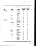 Methods
Table 4-26. Recommended Large Macroinvertebrate Species
for Bioaccumulation Monitoring
Region
Recommended Species3
Massachusetts to Virginia
Alaska to California
Florida, Virgin Islands, and Puerto Rico
Hawaii
American lobster (Homarus americanus)
Eastern rock crab (Cancer irroratus)
Hard clam (Mercenaria mercenaris)
Soft-shell clam (Mya arenaris)
Ocean quahog (Artica islandica)
Surf clam (Spisula solidissima)
Edible mussel (Mytilus edulis)
Spiny lobster (Panulirus interruptus)
Dungeness crab (Cancer magistei1)
Rock crab (Cancer antennarius)
Yellow crab (Cancer anthonyi)
Red crab (Cancer productus)
California mussel (Mytilus californianus)
Spiny lobster (Panulirus argus)
Spiny lobster (Panulirus penicillatus)
a Additional species that may occur at specific discharge sites and are considered acceptable
bioaccumulation monitoring species include the American oyster (Crassostrea virginica) and the Pacific
oyster (Crassostrea gigas).
A disadvantage of macroinvertebrates is the lack of adequate tissue biomass for
analyses. Adult fish are often used not only for their significant biomass, but also as a
measure of possible contaminants available to the human population. Fish, however,
are motile and may not be representative of the study area.
Ideally, studies should include samples of numerous species from many phyla. This
diversity will ensure the collection of bioaccumulation data for a wide spectrum of
contaminants and will indicate a species' potential to bioaccumulate those contaminants.
For example, oysters and other bivalves are ideal for monitoring bioaccumulation of
PAHs because of their limited ability to metabolically transform these contaminants. The
monitoring of a food chain could establish the potential for transport from one trophic
level to another. Species with extensive bioaccumulation data would be preferred. A
fundamental criterion is the ability to use the selected species to make comparisons
between sampling locations and sampling periods.
180
image:
Methods
Table 4-26. Recommended Large Macroinvertebrate Species
for Bioaccumulation Monitoring
Region
Recommended Species3
Massachusetts to Virginia
Alaska to California
Florida, Virgin Islands, and Puerto Rico
Hawaii
American lobster (Homarus americanus)
Eastern rock crab (Cancer irroratus)
Hard clam (Mercenaria mercenaris)
Soft-shell clam (Mya arenaris)
Ocean quahog (Artica islandica)
Surf clam (Spisula solidissima)
Edible mussel (Mytilus edulis)
Spiny lobster (Panulirus interruptus)
Dungeness crab (Cancer magistei1)
Rock crab (Cancer antennarius)
Yellow crab (Cancer anthonyi)
Red crab (Cancer productus)
California mussel (Mytilus californianus)
Spiny lobster (Panulirus argus)
Spiny lobster (Panulirus penicillatus)
a Additional species that may occur at specific discharge sites and are considered acceptable
bioaccumulation monitoring species include the American oyster (Crassostrea virginica) and the Pacific
oyster (Crassostrea gigas).
A disadvantage of macroinvertebrates is the lack of adequate tissue biomass for
analyses. Adult fish are often used not only for their significant biomass, but also as a
measure of possible contaminants available to the human population. Fish, however,
are motile and may not be representative of the study area.
Ideally, studies should include samples of numerous species from many phyla. This
diversity will ensure the collection of bioaccumulation data for a wide spectrum of
contaminants and will indicate a species' potential to bioaccumulate those contaminants.
For example, oysters and other bivalves are ideal for monitoring bioaccumulation of
PAHs because of their limited ability to metabolically transform these contaminants. The
monitoring of a food chain could establish the potential for transport from one trophic
level to another. Species with extensive bioaccumulation data would be preferred. A
fundamental criterion is the ability to use the selected species to make comparisons
between sampling locations and sampling periods.
180
image:
 Section 403 Procedural and Monitoring Guidance
Caged Indicator vs. Indigenous Species
The California Mussel Watch Program, the U.S. Mussel Watch Program, and the NOAA
Status and Trends Program have employed the use of both resident and caged
transplant mussels to monitor bioaccumulation of toxic chemicals over space and time
(Goldberg etal., 1978; Boehm, 1984; Ladd etal., 1984). Caged indicator target species
offer several advantages over indigenous species :
. The biology and ecology of these indicator species are usually well described.
• Descriptions of culture and/or maintenance of the organisms under laboratory
conditions are often available.
.• The method provides control of initial temporal and spatial variation of
individuals and/or biomass.
• The method allows the use of a specific age, size, and/or genetic stock.
• The method ensures on-site bioaccumulation.
By controlling for initial conditions, the rate of change of tissue contamination may be
calculated. In addition, the Long Island Sound National Estuary Program has shown
that performing chemical residue analyses on caged indicator species appears to be a
promising approach for identifying sources of pollution (USEPA, 1982c).
The use of a caged indicator species indicates only uptake due to exposure to the water
column, and unfortunately methods for caging sediment-ingesting organisms are not yet
available. The bioaccumulation of sediment-sorbed contaminants is thought to be
indicated by transfer through interstitial waters (Knezovich and Harrison, 1987), and the
results often do not relate to species found on site. Therefore, caged organisms may
not provide a full-spectrum profile of the contaminants that are bioavailable at any one
site.
The advantages of indigenous species are as follows:
• Results obtained will relate directly to those species which may be impacted
and will provide a direct measure of potential risks to human health.
• There is no cost of transplanting organisms.
• There is no possibility of loss of cage/buoy system.
• There is no possibility of introduction of a "nuisance" species.
Unfortunately, common indigenous species may not meet the criteria for use as
bioaccumulation target species, negating any advantage of using a native species. The
most common problem is collecting sufficient tissue biomass of appropriate species
181
image:
Section 403 Procedural and Monitoring Guidance
Caged Indicator vs. Indigenous Species
The California Mussel Watch Program, the U.S. Mussel Watch Program, and the NOAA
Status and Trends Program have employed the use of both resident and caged
transplant mussels to monitor bioaccumulation of toxic chemicals over space and time
(Goldberg etal., 1978; Boehm, 1984; Ladd etal., 1984). Caged indicator target species
offer several advantages over indigenous species :
. The biology and ecology of these indicator species are usually well described.
• Descriptions of culture and/or maintenance of the organisms under laboratory
conditions are often available.
.• The method provides control of initial temporal and spatial variation of
individuals and/or biomass.
• The method allows the use of a specific age, size, and/or genetic stock.
• The method ensures on-site bioaccumulation.
By controlling for initial conditions, the rate of change of tissue contamination may be
calculated. In addition, the Long Island Sound National Estuary Program has shown
that performing chemical residue analyses on caged indicator species appears to be a
promising approach for identifying sources of pollution (USEPA, 1982c).
The use of a caged indicator species indicates only uptake due to exposure to the water
column, and unfortunately methods for caging sediment-ingesting organisms are not yet
available. The bioaccumulation of sediment-sorbed contaminants is thought to be
indicated by transfer through interstitial waters (Knezovich and Harrison, 1987), and the
results often do not relate to species found on site. Therefore, caged organisms may
not provide a full-spectrum profile of the contaminants that are bioavailable at any one
site.
The advantages of indigenous species are as follows:
• Results obtained will relate directly to those species which may be impacted
and will provide a direct measure of potential risks to human health.
• There is no cost of transplanting organisms.
• There is no possibility of loss of cage/buoy system.
• There is no possibility of introduction of a "nuisance" species.
Unfortunately, common indigenous species may not meet the criteria for use as
bioaccumulation target species, negating any advantage of using a native species. The
most common problem is collecting sufficient tissue biomass of appropriate species
181
image:
 Methods
across sampling locations throughout the study. The composition of benthic community
species is subject to large natural fluctuations, as well as fluctuations in response to
pollution (Pearson and Rosenberg, 1978); indigenous species initially present may not
be available later, limiting temporal and spatial comparisons.
Selection of Tissues
The type and location of tissue analyzed will depend on the objectives of individual
monitoring programs. It is strongly recommended that all analyses be conducted with
the same species and tissue type in order that scientifically and statistically valid
comparisons may be made.
In fish, liver tissue is closely associated with regulation and storage of many toxic
substances (Fowler, 1982). Its high fatty tissue content tends to accumulate lipophilic
contaminants. Therefore, contaminant levels in the liver can be used to estimate the
range of contaminants being assimilated. For macroinvertebrates, hepatopancreas or
digestive gland tissue performs functions analogous to those of fish liver tissue.
Contaminants in edible muscle tissue represent those contaminants that are retained in
a form that allows transfer to humans. Sampling of muscle tissue is appropriate for
human exposure assessments and quantitative health risk determinations. Within a
fillet, contaminant concentrations may vary; therefore, it is recommended that a
consistent location within the muscle tissue be analyzed (USEPA, 1989a).
Whole-body analyses should be conducted when predators consume the whole body of
the target organism. If organisms are not cleansed of materials contained in the
digestive tract, contaminants in the gut contents will be included in the analyses. To
provide the most accurate estimate of the total amount of contaminants available to
most macroinvertebrate predators, this type of cleansing may not be required.
Total Organic Carbon and Acid Volatile Sulfides. and Tissue Lipid Normalization
Toxic sediment concentrations of hydrophobic contaminants have been found to be
related to the total organic carbon content (TOC) of the sediment (Karickhoff et al.,
1979). The bioavailability of metal contaminants has been found to be related to the
acid volatile sulfide (AVS) concentrations of the sediment (DiToro et al., in press). TOC
and AVS normalizations have been conducted to estimate the concentrations of
sediment contaminants that are bioavailable over different sampling locations.
Sediment TOC and AVS normalizations are recommended to account for the variability
in bioavailable sediment contaminant concentrations between locations.
Lipids appear to be a storage site of organochlorines, hydrocarbons, and other
hydrophobic contaminants in a variety of organisms (de Boer, 1988). In fact, just as
TOC and AVS are considered by many to be the most important parameters in defining
182
image:
Methods
across sampling locations throughout the study. The composition of benthic community
species is subject to large natural fluctuations, as well as fluctuations in response to
pollution (Pearson and Rosenberg, 1978); indigenous species initially present may not
be available later, limiting temporal and spatial comparisons.
Selection of Tissues
The type and location of tissue analyzed will depend on the objectives of individual
monitoring programs. It is strongly recommended that all analyses be conducted with
the same species and tissue type in order that scientifically and statistically valid
comparisons may be made.
In fish, liver tissue is closely associated with regulation and storage of many toxic
substances (Fowler, 1982). Its high fatty tissue content tends to accumulate lipophilic
contaminants. Therefore, contaminant levels in the liver can be used to estimate the
range of contaminants being assimilated. For macroinvertebrates, hepatopancreas or
digestive gland tissue performs functions analogous to those of fish liver tissue.
Contaminants in edible muscle tissue represent those contaminants that are retained in
a form that allows transfer to humans. Sampling of muscle tissue is appropriate for
human exposure assessments and quantitative health risk determinations. Within a
fillet, contaminant concentrations may vary; therefore, it is recommended that a
consistent location within the muscle tissue be analyzed (USEPA, 1989a).
Whole-body analyses should be conducted when predators consume the whole body of
the target organism. If organisms are not cleansed of materials contained in the
digestive tract, contaminants in the gut contents will be included in the analyses. To
provide the most accurate estimate of the total amount of contaminants available to
most macroinvertebrate predators, this type of cleansing may not be required.
Total Organic Carbon and Acid Volatile Sulfides. and Tissue Lipid Normalization
Toxic sediment concentrations of hydrophobic contaminants have been found to be
related to the total organic carbon content (TOC) of the sediment (Karickhoff et al.,
1979). The bioavailability of metal contaminants has been found to be related to the
acid volatile sulfide (AVS) concentrations of the sediment (DiToro et al., in press). TOC
and AVS normalizations have been conducted to estimate the concentrations of
sediment contaminants that are bioavailable over different sampling locations.
Sediment TOC and AVS normalizations are recommended to account for the variability
in bioavailable sediment contaminant concentrations between locations.
Lipids appear to be a storage site of organochlorines, hydrocarbons, and other
hydrophobic contaminants in a variety of organisms (de Boer, 1988). In fact, just as
TOC and AVS are considered by many to be the most important parameters in defining
182
image:
 Section 403 Procedural and Monitoring Guidance
organic and metal concentrations in sediments, lipid content is considered the salient
parameter in defining hydrophobic residue concentrations found in tissues (Phillips and
Segar, 1986). Likewise, tissue lipid normalizations have been suggested to account for
the variability in tissue contaminant concentrations between individuals.
Normalization of sediment contaminant concentrations to TOG and AVS and
normalization of tissue contaminant concentrations to the tissue lipid concentrations
have been made to permit comparisons of toxic chemical residues in tissues between
studies, locations, individuals, and tissue types. These sediment and tissue
normalizations assume the following::
• Contaminants partition predominantly to sediment TOC, sediment AVS, and
organismal lipids.
• Contaminants partition reversibly between the sediment particles and the
organism.
• Rapid steady-state kinetics of contaminants are maintained.
• Sediment is the only source for the bioaccumulation.
Lipid normalization has been performed in order that individuals with differing body fat
levels may be compared. Again, it is essential that all analyses be conducted with the
same tissue type from the same species to ensure that scientifically and statistically
valid comparisons may be made. TOC/lipid normalized accumulation factors (AF) have
also been used to predict tissue residue concentrations (Ferraro et al., 1990; Lake et al.,
1987).
Threefold differences in lipid concentration may result as a consequence of various lipid
analysis techniques. Development of protocol standardization or intercalibration
between lipid techniques is required before chemical residues in tissues can be
compared between studies, Microtechniques have been developed for analyses of
lipids from single individuals (Gardner et al., 1985). Finally, the decision to normalize for
TOC, AVS, and percent Ispid will depend on monitoring program objectives. For
example, if the monitoring objective is to identify "hot spots"—i.e., those areas where
high body burdens present a risk to human and ecological health—normalization may
not be appropriate. If the objective is to identify temporal trends in bioaccumulation
rates, however, normalization may be justified.
Selection of Sampling Period
The timing of sampling should be based on biological cycles that influence an
organism's susceptibility to bioaccumulation. For example, for crustaceans, just after
molting and before hardening of the integument occurs, restricting its permeability, there
is a significant increase in potential for bioaccumulation of toxic contaminants. The
183
image:
Section 403 Procedural and Monitoring Guidance
organic and metal concentrations in sediments, lipid content is considered the salient
parameter in defining hydrophobic residue concentrations found in tissues (Phillips and
Segar, 1986). Likewise, tissue lipid normalizations have been suggested to account for
the variability in tissue contaminant concentrations between individuals.
Normalization of sediment contaminant concentrations to TOG and AVS and
normalization of tissue contaminant concentrations to the tissue lipid concentrations
have been made to permit comparisons of toxic chemical residues in tissues between
studies, locations, individuals, and tissue types. These sediment and tissue
normalizations assume the following::
• Contaminants partition predominantly to sediment TOC, sediment AVS, and
organismal lipids.
• Contaminants partition reversibly between the sediment particles and the
organism.
• Rapid steady-state kinetics of contaminants are maintained.
• Sediment is the only source for the bioaccumulation.
Lipid normalization has been performed in order that individuals with differing body fat
levels may be compared. Again, it is essential that all analyses be conducted with the
same tissue type from the same species to ensure that scientifically and statistically
valid comparisons may be made. TOC/lipid normalized accumulation factors (AF) have
also been used to predict tissue residue concentrations (Ferraro et al., 1990; Lake et al.,
1987).
Threefold differences in lipid concentration may result as a consequence of various lipid
analysis techniques. Development of protocol standardization or intercalibration
between lipid techniques is required before chemical residues in tissues can be
compared between studies, Microtechniques have been developed for analyses of
lipids from single individuals (Gardner et al., 1985). Finally, the decision to normalize for
TOC, AVS, and percent Ispid will depend on monitoring program objectives. For
example, if the monitoring objective is to identify "hot spots"—i.e., those areas where
high body burdens present a risk to human and ecological health—normalization may
not be appropriate. If the objective is to identify temporal trends in bioaccumulation
rates, however, normalization may be justified.
Selection of Sampling Period
The timing of sampling should be based on biological cycles that influence an
organism's susceptibility to bioaccumulation. For example, for crustaceans, just after
molting and before hardening of the integument occurs, restricting its permeability, there
is a significant increase in potential for bioaccumulation of toxic contaminants. The
183
image:
 Methods
frequency of sampling should be related to the expected rate of change in tissue
concentrations of contaminants. A consistent sampling period is recommended in order
that spatial and temporal comparisons may be conducted.
For many aquatic vertebrate and invertebrate organisms, the reproductive cycle exerts a
major influence on tissue concentrations of many contaminants, especially lipophilic
compounds (Phillips, 1980). For many species, lipophilic contaminants are transferred
from the muscle and liver to the eggs as lipids are mobilized and transported to the egg
during oogenesis (Spies et al., 1988; Gardner et al., 1985). There is evidence that
lipophilic contaminants have deleterious effects on the developing egg and/or the larvae
(Spies et al., 1988; Hansen et al., 1985; Niimi, 1983). Transfer of contaminants from
adult to egg and its potential impacts on future fisheries recruitment and fisheries
production are under investigation.
It is recommended that target species be sampled when tissue contaminant
concentrations are expected to be at their highest levels in order to evaluate worst-case
scenarios. For those organisms where the body is consumed whole, contaminant levels
are usually at their highest at or just before spawning. For organisms where the muscle
tissue is consumed, contaminants in muscle tissue usually reach a peak well before
spawning.
4.10.3 Analytical Methods Considerations
Factors to be considered during the choice of an appropriate analytical method include
the parameters of interest, desired detection limits, sample size requirements or
restrictions, methods of preservation, technical and practical holding times, and matrix
interferences. Several USEPA documents (1986b, 1987c, 1990c) discuss the common
analytical problems encountered during monitoring analyses of tissue samples.
Chemical Residue Analyses
Several factors determine achievable detection limits for a specific contaminant,
regardless of analytical procedure. These factors include:
• Size of the tissue sample available for analysis. In general, the more tissue
available for analysis, the better the detection levels that can be achieved; a
minimum of 30 g (wet weight) is usually considered adequate (USEPA,
1987c);
• Presence of interfering substances;
• Range of pollutants to be analyzed—an optimal method may be developed
without regard to potential effects on other parameters;
• Level of confirmation—qualitative vs. quantitative analyses; and
184
image:
Methods
frequency of sampling should be related to the expected rate of change in tissue
concentrations of contaminants. A consistent sampling period is recommended in order
that spatial and temporal comparisons may be conducted.
For many aquatic vertebrate and invertebrate organisms, the reproductive cycle exerts a
major influence on tissue concentrations of many contaminants, especially lipophilic
compounds (Phillips, 1980). For many species, lipophilic contaminants are transferred
from the muscle and liver to the eggs as lipids are mobilized and transported to the egg
during oogenesis (Spies et al., 1988; Gardner et al., 1985). There is evidence that
lipophilic contaminants have deleterious effects on the developing egg and/or the larvae
(Spies et al., 1988; Hansen et al., 1985; Niimi, 1983). Transfer of contaminants from
adult to egg and its potential impacts on future fisheries recruitment and fisheries
production are under investigation.
It is recommended that target species be sampled when tissue contaminant
concentrations are expected to be at their highest levels in order to evaluate worst-case
scenarios. For those organisms where the body is consumed whole, contaminant levels
are usually at their highest at or just before spawning. For organisms where the muscle
tissue is consumed, contaminants in muscle tissue usually reach a peak well before
spawning.
4.10.3 Analytical Methods Considerations
Factors to be considered during the choice of an appropriate analytical method include
the parameters of interest, desired detection limits, sample size requirements or
restrictions, methods of preservation, technical and practical holding times, and matrix
interferences. Several USEPA documents (1986b, 1987c, 1990c) discuss the common
analytical problems encountered during monitoring analyses of tissue samples.
Chemical Residue Analyses
Several factors determine achievable detection limits for a specific contaminant,
regardless of analytical procedure. These factors include:
• Size of the tissue sample available for analysis. In general, the more tissue
available for analysis, the better the detection levels that can be achieved; a
minimum of 30 g (wet weight) is usually considered adequate (USEPA,
1987c);
• Presence of interfering substances;
• Range of pollutants to be analyzed—an optimal method may be developed
without regard to potential effects on other parameters;
• Level of confirmation—qualitative vs. quantitative analyses; and
184
image:
 Section 403 Procedural and Monitoring Guidance
• Level of pollutant found in the field and in analytical blanks.
Selection of appropriate methods ought to be based on a trade-off between full-scan
analyses, which are economical but cannot provide optimal sensitivity for some
compounds, and alternative methods that are more sensitive for specific compounds but
can result in higher analytical costs. A list of analytical techniques is presented in Table
4-27.
The Computerized Risk and Bioaccumulation System (CRABS, Version 1.0) is an expert
system designed to predict tissue residues of 15 neutral organic pollutants in
sediment-dwelling organisms and the human cancer risk from consumption of
contaminated shellfish (USEPA, 1990c). Thermodynamic partitioning, first-order
kinetics, or toxicokinetic models are used to predict bioaccumulation from bedded
sediment. Steady-state tissue residues are predicted from any of the models, whereas
the two kinetic models are used to predict either non-steady-state uptake or elimination.
The lifetime human cancer risk is then predicted for the consumption of clams and other
nonmobile sediment-dwelling organisms containing the predicted or measured tissue
residue. The cancer risk is predicted for a single pollutant from a single-species diet.
Shellfish consumption rates can be estimated if site-specific rates are available.
Table 4-27. List of Analytical Techniques (USEPA, 1986b)
METALS/METALLOIDS
• Atomic Absorption Spectrophotometry (AA) USEPA 7000 series methods
flame
graphite furnace (GFAA)
cold vapor
gaseous hydride (HYDAA)
USEPA method 7470
USEPA methods 7060 and 7740
• Inductively Coupled Plasma Emission Spectrometry (ICP) USEPA method 6010
ORGANICS
• Gas Chromatography (GC)
with electron capture detection (GC/ECD)
with mass spectrometry (GC/MS)
USEPA method 8080
USEPA methods 8240 and 8270
SOURCE: USEPA, 1986b.
185
image:
Section 403 Procedural and Monitoring Guidance
• Level of pollutant found in the field and in analytical blanks.
Selection of appropriate methods ought to be based on a trade-off between full-scan
analyses, which are economical but cannot provide optimal sensitivity for some
compounds, and alternative methods that are more sensitive for specific compounds but
can result in higher analytical costs. A list of analytical techniques is presented in Table
4-27.
The Computerized Risk and Bioaccumulation System (CRABS, Version 1.0) is an expert
system designed to predict tissue residues of 15 neutral organic pollutants in
sediment-dwelling organisms and the human cancer risk from consumption of
contaminated shellfish (USEPA, 1990c). Thermodynamic partitioning, first-order
kinetics, or toxicokinetic models are used to predict bioaccumulation from bedded
sediment. Steady-state tissue residues are predicted from any of the models, whereas
the two kinetic models are used to predict either non-steady-state uptake or elimination.
The lifetime human cancer risk is then predicted for the consumption of clams and other
nonmobile sediment-dwelling organisms containing the predicted or measured tissue
residue. The cancer risk is predicted for a single pollutant from a single-species diet.
Shellfish consumption rates can be estimated if site-specific rates are available.
Table 4-27. List of Analytical Techniques (USEPA, 1986b)
METALS/METALLOIDS
• Atomic Absorption Spectrophotometry (AA) USEPA 7000 series methods
flame
graphite furnace (GFAA)
cold vapor
gaseous hydride (HYDAA)
USEPA method 7470
USEPA methods 7060 and 7740
• Inductively Coupled Plasma Emission Spectrometry (ICP) USEPA method 6010
ORGANICS
• Gas Chromatography (GC)
with electron capture detection (GC/ECD)
with mass spectrometry (GC/MS)
USEPA method 8080
USEPA methods 8240 and 8270
SOURCE: USEPA, 1986b.
185
image:
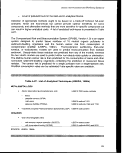 Methods
This program is now available for distribution. All inquiries should be directed to the
Narragansett, Rhode Island, Environmental Research Laboratory (Hatfield Marine
Science Center, Newport, OR 97365, 503/867-4042).
Tissue residue data necessary for the evaluation of dredged materials and for ecological
and human risk assessments are most directly derived using bedded sediments (i.e.,
deposited rather than suspended sediments) in bioaccumulation tests (USEPA, 1989d).
Sediments are the largest receiving grounds for toxics known to bind with particles, such
as organics with high octanol-water partitioning coefficients (e.g., PCBs and DDT) and
many heavy metals. Previous techniques have varied to meet specific requirements for
the task at hand, and comparability of results is questionable. USEPA (1989d)
standardizes an approach for conducting sediment bioaccumulation tests using
sediment-ingesting organisms exposed to bedded marine sediments. Guidance is
presented for "routine" testing in the laboratory and has not been tailored for specific
regulations or geographic locations. Data can be generated by the 28-day test that is
applicable for quantitative ecological and human health risk assessments. It should be
noted that this is a "living" document subject to revisions warranted by experience.
Metals and Metalloids
Nitric acid/perchloric acid digestions should be considered for analysis of tissue
samples. Perchloric acid is especially useful for the dissolution of fat.
Trace element analyses by inductively coupled plasma emission spectrometry (ICP)
allow for several elements to be measured simultaneously. However, the detection
limits of ICP are generally not as sensitive as those achieved by graphite furnace atomic
absorption spectrophotometry (GFAA).
The combination of atomic absorption spectrophotometry techniques (AA) and ICP is
the recommended analytical method for detection of metals and metalloids since no
technique is best for all elements. Cold vapor AA analysis is the only recommended
technique for mercury.
GFAA is more sensitive than flame AA, but is more subject to matrix and spectral
influences. GFAA requires particular caution with regard to laboratory contamination. In
either case, the concentration of each element is determined by a separate analysis,
making the analysis of a large number of contaminant metals both labor-intensive and
relatively expensive compared to ICP.
Semivolatile Organic Compounds
Analysis of semivolatile organic compounds involves a solvent extraction of the sample,
cleanup of the characteristically complex extract, and gas chromatography (GC)
analysis and quantification. There are two gas chromatography/mass spectrometry
186
image:
Methods
This program is now available for distribution. All inquiries should be directed to the
Narragansett, Rhode Island, Environmental Research Laboratory (Hatfield Marine
Science Center, Newport, OR 97365, 503/867-4042).
Tissue residue data necessary for the evaluation of dredged materials and for ecological
and human risk assessments are most directly derived using bedded sediments (i.e.,
deposited rather than suspended sediments) in bioaccumulation tests (USEPA, 1989d).
Sediments are the largest receiving grounds for toxics known to bind with particles, such
as organics with high octanol-water partitioning coefficients (e.g., PCBs and DDT) and
many heavy metals. Previous techniques have varied to meet specific requirements for
the task at hand, and comparability of results is questionable. USEPA (1989d)
standardizes an approach for conducting sediment bioaccumulation tests using
sediment-ingesting organisms exposed to bedded marine sediments. Guidance is
presented for "routine" testing in the laboratory and has not been tailored for specific
regulations or geographic locations. Data can be generated by the 28-day test that is
applicable for quantitative ecological and human health risk assessments. It should be
noted that this is a "living" document subject to revisions warranted by experience.
Metals and Metalloids
Nitric acid/perchloric acid digestions should be considered for analysis of tissue
samples. Perchloric acid is especially useful for the dissolution of fat.
Trace element analyses by inductively coupled plasma emission spectrometry (ICP)
allow for several elements to be measured simultaneously. However, the detection
limits of ICP are generally not as sensitive as those achieved by graphite furnace atomic
absorption spectrophotometry (GFAA).
The combination of atomic absorption spectrophotometry techniques (AA) and ICP is
the recommended analytical method for detection of metals and metalloids since no
technique is best for all elements. Cold vapor AA analysis is the only recommended
technique for mercury.
GFAA is more sensitive than flame AA, but is more subject to matrix and spectral
influences. GFAA requires particular caution with regard to laboratory contamination. In
either case, the concentration of each element is determined by a separate analysis,
making the analysis of a large number of contaminant metals both labor-intensive and
relatively expensive compared to ICP.
Semivolatile Organic Compounds
Analysis of semivolatile organic compounds involves a solvent extraction of the sample,
cleanup of the characteristically complex extract, and gas chromatography (GC)
analysis and quantification. There are two gas chromatography/mass spectrometry
186
image:
 Section 403 Procedural and Monitoring Guidance
(GC/MS) options for detecting extractable organic compounds: internal standard
technique and isotope dilution. Isotope dilution is recommended because reliable
recovery corrections can be made for each analyte with a labeled analog or a chemically
similar analog (Tetra Tech, 1986).
The identification of pesticides and PCB can be made by gas chromatography/electron
capture detection (GC/ECD) analysis. GC/ECD provides greater sensitivity relative to
GC/MS; however, GC/ECD does not provide positive compound identification.
Confirmation of pesticides and PCBs on an alternative GC/ECD column or preferably by
GC/MS, when sufficient concentrations occur, is recommended for reliable results (Tetra
Tech, 1985). All other organic compound groups are recommended for analysis by
GC/MS (Tetra Tech, 1985).
Volatile Organic Compounds
The purge-and-trap GC/MS technique is employed for detecting volatile organic
compounds in water. A successful variation for detection of volatile organic residues in
tissues involves a device that vaporizes volatile organic compounds from the tissue
sample under vacuum and then condenses the volatiles in a super-cooled trap (Hiatt,
1981). The trap is then transferred to a purge-and-trap device, where it is treated as a
water sample. The isotope dilution option is recommended because it provides reliable
recovery data for each analyte (Tetra Tech, 1986).
4.10.4 QA/QC Considerations
Analysis of blanks should be conducted to demonstrate freedom from contamination. At
least one method blank must be included with each batch of samples and must
constitute at least 5 percent of all samples analyzed.
Spike recovery analyses are required to assess method performance on the sample
matrix. This method serves as an indication of analytical accuracy, but not necessarily
of extraction efficiency.
Replicates must be analyzed to monitor the precision of laboratory analyses. A
minimum of 5 percent of the analyses should be laboratory replicates. Triplicates should
be performed with each sample batch over 40 samples.
Laboratory performance and calibration should be verified at the beginning and end of
each 12-hr shift during which analyses are performed.
Reports delineating the essential elements of the bioaccumulation component of the
program should be included with the quantitative QA/QC analyses. It is recommended
that these reports be recorded and stored in a data base for future reference.
187
image:
Section 403 Procedural and Monitoring Guidance
(GC/MS) options for detecting extractable organic compounds: internal standard
technique and isotope dilution. Isotope dilution is recommended because reliable
recovery corrections can be made for each analyte with a labeled analog or a chemically
similar analog (Tetra Tech, 1986).
The identification of pesticides and PCB can be made by gas chromatography/electron
capture detection (GC/ECD) analysis. GC/ECD provides greater sensitivity relative to
GC/MS; however, GC/ECD does not provide positive compound identification.
Confirmation of pesticides and PCBs on an alternative GC/ECD column or preferably by
GC/MS, when sufficient concentrations occur, is recommended for reliable results (Tetra
Tech, 1985). All other organic compound groups are recommended for analysis by
GC/MS (Tetra Tech, 1985).
Volatile Organic Compounds
The purge-and-trap GC/MS technique is employed for detecting volatile organic
compounds in water. A successful variation for detection of volatile organic residues in
tissues involves a device that vaporizes volatile organic compounds from the tissue
sample under vacuum and then condenses the volatiles in a super-cooled trap (Hiatt,
1981). The trap is then transferred to a purge-and-trap device, where it is treated as a
water sample. The isotope dilution option is recommended because it provides reliable
recovery data for each analyte (Tetra Tech, 1986).
4.10.4 QA/QC Considerations
Analysis of blanks should be conducted to demonstrate freedom from contamination. At
least one method blank must be included with each batch of samples and must
constitute at least 5 percent of all samples analyzed.
Spike recovery analyses are required to assess method performance on the sample
matrix. This method serves as an indication of analytical accuracy, but not necessarily
of extraction efficiency.
Replicates must be analyzed to monitor the precision of laboratory analyses. A
minimum of 5 percent of the analyses should be laboratory replicates. Triplicates should
be performed with each sample batch over 40 samples.
Laboratory performance and calibration should be verified at the beginning and end of
each 12-hr shift during which analyses are performed.
Reports delineating the essential elements of the bioaccumulation component of the
program should be included with the quantitative QA/QC analyses. It is recommended
that these reports be recorded and stored in a data base for future reference.
187
image:
 Methods
4.10.5 Statistical Design Considerations
Composite Sampling
Composite tissue sampling consists of mixing tissue samples from two or more
individual organisms, typically of a single species, collected at a particular location and
time period. The analysis of a composite sample provides an estimate of an average
tissue concentration for the individual organisms composing the composite sample.
Advantages of the composite sampling strategy are :
• It provides a cost-effective strategy when individual chemical analyses are
expensive.
• It provides a means to analyze bioaccumulation when the tissue mass of an
individual is insufficient for the analytical protocol.
• It results in a more efficient estimate of the mean at specified sampling
locations.
Because of the reduced sample variance, composite sampling results in a considerable
increase in statistical power. If the primary objective of a monitoring program is to
determine differences in contaminant tissue among sampling locations, composite
sampling is an appropriate strategy.
Composite sampling is not recommended if the objective of the monitoring program is to
determine compliance with specified tissue contaminant concentration limits since this
sampling method does not detect the true range of tissue contaminant concentrations in
the population. Special considerations related to composite sampling include :
• The range and the variance of the population of individual samples cannot be
directly estimated.
• If species are mixed, tissue composites are likely to be composed of different
proportions of species and numbers of individuals, confounding whether
patterns of tissue residue concentrations are due to differences in locations or
to interspecific differences in bioaccumulation.
Space-bulking consists of sampling of individual organisms from several locations and
combining tissue samples into one or more composite samples. Time-bulking involves
taking multiple samples over time from a single location and compositing these samples.
The use of space- and/or time-bulking strategies should be carefully considered since
significant information concerning spatial and temporal heterogeneity may be lost. The
adoption of composite strategies will depend on the objective of individual monitoring
programs.
188
image:
Methods
4.10.5 Statistical Design Considerations
Composite Sampling
Composite tissue sampling consists of mixing tissue samples from two or more
individual organisms, typically of a single species, collected at a particular location and
time period. The analysis of a composite sample provides an estimate of an average
tissue concentration for the individual organisms composing the composite sample.
Advantages of the composite sampling strategy are :
• It provides a cost-effective strategy when individual chemical analyses are
expensive.
• It provides a means to analyze bioaccumulation when the tissue mass of an
individual is insufficient for the analytical protocol.
• It results in a more efficient estimate of the mean at specified sampling
locations.
Because of the reduced sample variance, composite sampling results in a considerable
increase in statistical power. If the primary objective of a monitoring program is to
determine differences in contaminant tissue among sampling locations, composite
sampling is an appropriate strategy.
Composite sampling is not recommended if the objective of the monitoring program is to
determine compliance with specified tissue contaminant concentration limits since this
sampling method does not detect the true range of tissue contaminant concentrations in
the population. Special considerations related to composite sampling include :
• The range and the variance of the population of individual samples cannot be
directly estimated.
• If species are mixed, tissue composites are likely to be composed of different
proportions of species and numbers of individuals, confounding whether
patterns of tissue residue concentrations are due to differences in locations or
to interspecific differences in bioaccumulation.
Space-bulking consists of sampling of individual organisms from several locations and
combining tissue samples into one or more composite samples. Time-bulking involves
taking multiple samples over time from a single location and compositing these samples.
The use of space- and/or time-bulking strategies should be carefully considered since
significant information concerning spatial and temporal heterogeneity may be lost. The
adoption of composite strategies will depend on the objective of individual monitoring
programs.
188
image:
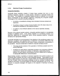 Section 403 Procedural and Monitoring Guidance
Statistical Power
Tetra Tech (1987) demonstrated that the statistical power increases with the increase of
the number of individuals in each replicate composite sample. However, a diminished
return of statistical power exists with the addition of successive individuals to each
composite. For composites of greater than 10 individuals, the increase of power is
negligible given typical levels of data variability.
For moderate levels of variability in chemical residue data, 6 to 10 individuals composing
each of 5 replicate composites should be adequate to detect a treatment difference
equal to 100 percent of the overall mean among treatments (Tetra Tech, 1987). For
analyses of individuals, a minimum of five organisms at each site is recommended.
To improve the power of a statistical test, while keeping the significance level constant,
the sample size should be increased. Because of constraints in cost and time, however,
this option may not be available. Power analyses have shown that for a fixed level of
sampling effort, a monitoring program's power is generally increased by collecting more
replicates at fewer locations. The number and distribution of sampling locations
required to evaluate the effect of a discharge will depend on the volume and transport of
the effluent.
4.10.6 Use of Data
Results of the bioaccumulation analyses can be used to :
• Establish spatial and temporal trends in the bioaccumulation of toxicants of
selected marine fish and macroinvertebrates;
• Identify existing arid potential problem areas for fish and macroinvertebrate
contamination; and
• Supply data that can be used to calculate the human health risk of
consuming marine fish and shellfish.
4.10.7 Summary
Rationale
• Monitoring the accumulation of chemical residues in tissues of marine
organisms will provide information essential in relating the presence of
selected contaminants in marine waters and sediment to their transfer and
accumulation in marine organisms.
189
image:
Section 403 Procedural and Monitoring Guidance
Statistical Power
Tetra Tech (1987) demonstrated that the statistical power increases with the increase of
the number of individuals in each replicate composite sample. However, a diminished
return of statistical power exists with the addition of successive individuals to each
composite. For composites of greater than 10 individuals, the increase of power is
negligible given typical levels of data variability.
For moderate levels of variability in chemical residue data, 6 to 10 individuals composing
each of 5 replicate composites should be adequate to detect a treatment difference
equal to 100 percent of the overall mean among treatments (Tetra Tech, 1987). For
analyses of individuals, a minimum of five organisms at each site is recommended.
To improve the power of a statistical test, while keeping the significance level constant,
the sample size should be increased. Because of constraints in cost and time, however,
this option may not be available. Power analyses have shown that for a fixed level of
sampling effort, a monitoring program's power is generally increased by collecting more
replicates at fewer locations. The number and distribution of sampling locations
required to evaluate the effect of a discharge will depend on the volume and transport of
the effluent.
4.10.6 Use of Data
Results of the bioaccumulation analyses can be used to :
• Establish spatial and temporal trends in the bioaccumulation of toxicants of
selected marine fish and macroinvertebrates;
• Identify existing arid potential problem areas for fish and macroinvertebrate
contamination; and
• Supply data that can be used to calculate the human health risk of
consuming marine fish and shellfish.
4.10.7 Summary
Rationale
• Monitoring the accumulation of chemical residues in tissues of marine
organisms will provide information essential in relating the presence of
selected contaminants in marine waters and sediment to their transfer and
accumulation in marine organisms.
189
image:
 Methods
Monitoring Design Considerations
• Target species should possess the following characteristics :
- high bioaccumulation potential for selected contaminants of concern;
- weak or absent metabolic regulation of selected contaminants;
- abundant enough, temporally and spatially, to allow for adequate
sampling;
- large enough to provide adequate amounts of tissue for analysis;
- sessile or sedentary in nature to ensure bioaccumulation is representative
of the study area; and
- easily collected.
• Caged indicator species
- Method allows for control of initial temporal and spatial variation of
individuals and/or biomass.
- Method allows for the use of specific age, size, and/or genetic stocks.
• Indigenous species
- Results obtained will relate directly to those species that may be impacted.
• Target tissues
- Fish liver or macroinvertebrate hepatopancreas analyses may be used to
estimate the range of contaminants being assimilated.
- Muscle tissue analyses are appropriate for human exposure assessments
and quantitative health risk determinations.
- Whole-body analyses should to be conducted when predators consume
the whole body of the target organism.
• TOC/Lipid Normalization
- Allow comparisons of chemical residue concentrations in tissues between
locations, individuals, and tissue type.
- Limitations in use due to differences in lipid analysis techniques.
Time of Sampling
- Timing of sampling should be based on biological cycles that influence an
organism's susceptibility to bioaccumulate.
- It is recommended that target species be sampled when tissue
contamination concentrations are expected to be at their highest level.
190
image:
Methods
Monitoring Design Considerations
• Target species should possess the following characteristics :
- high bioaccumulation potential for selected contaminants of concern;
- weak or absent metabolic regulation of selected contaminants;
- abundant enough, temporally and spatially, to allow for adequate
sampling;
- large enough to provide adequate amounts of tissue for analysis;
- sessile or sedentary in nature to ensure bioaccumulation is representative
of the study area; and
- easily collected.
• Caged indicator species
- Method allows for control of initial temporal and spatial variation of
individuals and/or biomass.
- Method allows for the use of specific age, size, and/or genetic stocks.
• Indigenous species
- Results obtained will relate directly to those species that may be impacted.
• Target tissues
- Fish liver or macroinvertebrate hepatopancreas analyses may be used to
estimate the range of contaminants being assimilated.
- Muscle tissue analyses are appropriate for human exposure assessments
and quantitative health risk determinations.
- Whole-body analyses should to be conducted when predators consume
the whole body of the target organism.
• TOC/Lipid Normalization
- Allow comparisons of chemical residue concentrations in tissues between
locations, individuals, and tissue type.
- Limitations in use due to differences in lipid analysis techniques.
Time of Sampling
- Timing of sampling should be based on biological cycles that influence an
organism's susceptibility to bioaccumulate.
- It is recommended that target species be sampled when tissue
contamination concentrations are expected to be at their highest level.
190
image:
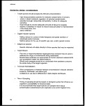 Section 403 Procedural and Monitoring Guidance
Analytical Methods Considerations
• Metals/Metalloids
- A combination of AA and IGP is recommended for the detection of metals
and metalloids.
- Cold vapor AA is the recommended protocol for mercury detection.
• Organics
- GC/MS in conjunction with isotope dilution is recommended for the
detection of semi volatile organic compounds.
- Super-cooled trap, in conjunction with a purge-and-trap device, is
recommended for the detection of volatile organics.
QA/QC Considerations
• Blank, spike recovery, and replicate analyses are recommended quality
control checks.
• Reports delineating the essential elements of the bioaccumulation
component of the program should be included with the quantitative QA/QC
analyses.
Statistical Design Considerations
• Compositing tissue sampling consists of mixing tissue samples from two or
more individual organisms collected at a particular location and time period.
• Space-bulking (combining composites from several locations) and
time-bulking (combining several composites over time from one location)
strategies should be used judiciously because information concerning spatial
and temporal heterogeneity may be lost.
• Six individuals composing each of five replicate composites should be
adequate to detect a treatment difference equal to 100 percent of the overall
mean among treatments.
Use of Data
• Establish spatial and temporal trends in the bioaccumulation of toxicants of
selected marine fish and macroinvertebrates.
• Identify existing arid potential problem areas for fish and macroinvertebrate
contamination.
• Supply data that can be used to calculate the human health risk of
consuming marine fish and shellfish.
191
image:
Section 403 Procedural and Monitoring Guidance
Analytical Methods Considerations
• Metals/Metalloids
- A combination of AA and IGP is recommended for the detection of metals
and metalloids.
- Cold vapor AA is the recommended protocol for mercury detection.
• Organics
- GC/MS in conjunction with isotope dilution is recommended for the
detection of semi volatile organic compounds.
- Super-cooled trap, in conjunction with a purge-and-trap device, is
recommended for the detection of volatile organics.
QA/QC Considerations
• Blank, spike recovery, and replicate analyses are recommended quality
control checks.
• Reports delineating the essential elements of the bioaccumulation
component of the program should be included with the quantitative QA/QC
analyses.
Statistical Design Considerations
• Compositing tissue sampling consists of mixing tissue samples from two or
more individual organisms collected at a particular location and time period.
• Space-bulking (combining composites from several locations) and
time-bulking (combining several composites over time from one location)
strategies should be used judiciously because information concerning spatial
and temporal heterogeneity may be lost.
• Six individuals composing each of five replicate composites should be
adequate to detect a treatment difference equal to 100 percent of the overall
mean among treatments.
Use of Data
• Establish spatial and temporal trends in the bioaccumulation of toxicants of
selected marine fish and macroinvertebrates.
• Identify existing arid potential problem areas for fish and macroinvertebrate
contamination.
• Supply data that can be used to calculate the human health risk of
consuming marine fish and shellfish.
191
image:
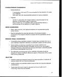 Methods
4.11 PATHOGENS
Monitoring for pathogenic microorganisms is currently conducted by State environmental
and human health agencies in shellfish harvesting areas and bathing beaches. National
Pollutant Discharge Elimination System (NPDES) pathogen monitoring programs may
be under way at selected locations both to assess the condition of water in the vicinity of
discharges and surrounding areas and to assess relative pathogen contributions from
these permitted effluent discharges.
The National Shellfish Sanitation Program (NSSP) has been established as a joint effort
involving the Food and Drug Administration (FDA), State agencies, and the shellfish
industry to set forth guidelines for the management of State shellfish programs. As part
of the NSSP, the Food and Drug Administration (FDA) provides technical assistance to
States for studying specific pollution problems, provides data to establish closure levels
for shellfish harvesting, conducts applied research on various contaminants to assist in
developing standards and criteria, and evaluates the effectiveness of State shellfish
sanitary control programs. In addition, since 1966, data have been compiled periodically
by FDA and the National Oceanic and Atmospheric Administration (NOAA) on the
classification by States of coastal and estuarine waters with regard to suitability for
shellfishing activities. In addition to classifying their waters as to their suitability as
shellfish harvesting areas, States also issue beach closures. These closures are
typically based on water quality criteria developed by the Federal government.
4.11.1 Rationale
Monitoring of pathogens in the marine environment can be used in the CWA section 403
point source discharge program to address the following ocean discharge guideline:
• Potential direct or indirect impacts on human health.
Human pathogens found in the marine environment include viruses, bacteria,
protozoans, helminth and parasites. In the United States, viruses and bacteria are the
most important pathogens, in terms of both the number of organisms released to the
environment and the severity of the diseases they cause (OTA, 1987).
Humans can be exposed to pathogens by direct contact with contaminated waters (e.g.,
swimming, surfing, diving) or indirectly through ingestion of contaminated food (e.g.,
molluscan shellfish). The preponderance of evidence indicates that the etiologic agents
for waterborne outbreaks of acute gastroenteritis (AGI) are the Norwalk-like viruses
(Kaplan et al. 1982). Hepatitis A has been linked to the consumption of raw or partially
cooked molluscan shellfish (Feingold, 1973; CDC, 1979; Ohara et al., 1983). Bacteria
responsible for typhoid and cholera are known to be water- and seafood-borne. These
pathogens can enter the marine environment through the discharge of raw sewage,
wastewater effluent from sewage treatment plants, failing septic tanks, and the dumping
of sewage sludge (OTA, 1987). Monitoring of human pathogens provides information
192
image:
Methods
4.11 PATHOGENS
Monitoring for pathogenic microorganisms is currently conducted by State environmental
and human health agencies in shellfish harvesting areas and bathing beaches. National
Pollutant Discharge Elimination System (NPDES) pathogen monitoring programs may
be under way at selected locations both to assess the condition of water in the vicinity of
discharges and surrounding areas and to assess relative pathogen contributions from
these permitted effluent discharges.
The National Shellfish Sanitation Program (NSSP) has been established as a joint effort
involving the Food and Drug Administration (FDA), State agencies, and the shellfish
industry to set forth guidelines for the management of State shellfish programs. As part
of the NSSP, the Food and Drug Administration (FDA) provides technical assistance to
States for studying specific pollution problems, provides data to establish closure levels
for shellfish harvesting, conducts applied research on various contaminants to assist in
developing standards and criteria, and evaluates the effectiveness of State shellfish
sanitary control programs. In addition, since 1966, data have been compiled periodically
by FDA and the National Oceanic and Atmospheric Administration (NOAA) on the
classification by States of coastal and estuarine waters with regard to suitability for
shellfishing activities. In addition to classifying their waters as to their suitability as
shellfish harvesting areas, States also issue beach closures. These closures are
typically based on water quality criteria developed by the Federal government.
4.11.1 Rationale
Monitoring of pathogens in the marine environment can be used in the CWA section 403
point source discharge program to address the following ocean discharge guideline:
• Potential direct or indirect impacts on human health.
Human pathogens found in the marine environment include viruses, bacteria,
protozoans, helminth and parasites. In the United States, viruses and bacteria are the
most important pathogens, in terms of both the number of organisms released to the
environment and the severity of the diseases they cause (OTA, 1987).
Humans can be exposed to pathogens by direct contact with contaminated waters (e.g.,
swimming, surfing, diving) or indirectly through ingestion of contaminated food (e.g.,
molluscan shellfish). The preponderance of evidence indicates that the etiologic agents
for waterborne outbreaks of acute gastroenteritis (AGI) are the Norwalk-like viruses
(Kaplan et al. 1982). Hepatitis A has been linked to the consumption of raw or partially
cooked molluscan shellfish (Feingold, 1973; CDC, 1979; Ohara et al., 1983). Bacteria
responsible for typhoid and cholera are known to be water- and seafood-borne. These
pathogens can enter the marine environment through the discharge of raw sewage,
wastewater effluent from sewage treatment plants, failing septic tanks, and the dumping
of sewage sludge (OTA, 1987). Monitoring of human pathogens provides information
192
image:
 Section 403 Procedural and Monitoring Guidance
essential in relating the presence of pathogens in marine waters and shellfish to
outbreaks of disease. Monitoring data may be used to identify potential sources of
pathogens. The assessment of pathogen contamination should be a component of a
monitoring program where pathogens may present a risk to human health and the
economic vitality of the marine environment.
4.11.2 Monitoring Design Considerations
Water Column Sampling
Bacteria are not uniformly distributed throughout the water column (Gameson, 1983);
bacterial abundances, several orders of magnitude greater than underlying waters, can
be found in a thin microlayer on the surface of the water (Hardy, 1982). If feasible, it is
recommended that samples of this microlayer and separate samples of the underlying
waters be collected. However, standardized methods for sampling this microlayer have
not been established. If it is not feasible to sample both the microlayer and underlying
waters, the "scoop" method should be used to ensure that the surface microlayer is
sampled (USEPA, 1978).
Water samples for bacterial analyses are frequently collected using sterilized plastic
bags (e.g., Whirl-Pak) or screw-cap, wide-mouthed bottles. Several depths may be
sampled during one cast, and/or replicate samples may be collected at a particular
depth by using Kemmerer or Niskin samplers (USEPA, 1978). Any device that collects
water samples in unsterilized tubes should not be used for collecting bacteriological
samples without first obtaining data that support its use. Pumps may be used to sample
large volumes of the water column (USEPA, 1978).
Sentinel Organisms
Analyses of sentinel shellfish tissue (e.g., mussels and oysters) offer several
advantages:
• They concentrate pathogens and may be useful viral analyses since viruses
are often present in low numbers.
• They provide a means of temporally integrating water quality conditions.
• They may be direct measures of human exposure to pathogens (i.e.,
consumption of contaminated food).
• They may be deployed and maintained in a number of diverse locales.
However, the disadvantages of sentinel organisms include:
• Transplanting organisms may be costly;
193
image:
Section 403 Procedural and Monitoring Guidance
essential in relating the presence of pathogens in marine waters and shellfish to
outbreaks of disease. Monitoring data may be used to identify potential sources of
pathogens. The assessment of pathogen contamination should be a component of a
monitoring program where pathogens may present a risk to human health and the
economic vitality of the marine environment.
4.11.2 Monitoring Design Considerations
Water Column Sampling
Bacteria are not uniformly distributed throughout the water column (Gameson, 1983);
bacterial abundances, several orders of magnitude greater than underlying waters, can
be found in a thin microlayer on the surface of the water (Hardy, 1982). If feasible, it is
recommended that samples of this microlayer and separate samples of the underlying
waters be collected. However, standardized methods for sampling this microlayer have
not been established. If it is not feasible to sample both the microlayer and underlying
waters, the "scoop" method should be used to ensure that the surface microlayer is
sampled (USEPA, 1978).
Water samples for bacterial analyses are frequently collected using sterilized plastic
bags (e.g., Whirl-Pak) or screw-cap, wide-mouthed bottles. Several depths may be
sampled during one cast, and/or replicate samples may be collected at a particular
depth by using Kemmerer or Niskin samplers (USEPA, 1978). Any device that collects
water samples in unsterilized tubes should not be used for collecting bacteriological
samples without first obtaining data that support its use. Pumps may be used to sample
large volumes of the water column (USEPA, 1978).
Sentinel Organisms
Analyses of sentinel shellfish tissue (e.g., mussels and oysters) offer several
advantages:
• They concentrate pathogens and may be useful viral analyses since viruses
are often present in low numbers.
• They provide a means of temporally integrating water quality conditions.
• They may be direct measures of human exposure to pathogens (i.e.,
consumption of contaminated food).
• They may be deployed and maintained in a number of diverse locales.
However, the disadvantages of sentinel organisms include:
• Transplanting organisms may be costly;
193
image:
 Methods
There is a possibility of losing the cage/buoy system; and
Species may not be tolerant of all test site conditions (e.g., low salinity, high
turbidity).
It is essential that monitoring design elements be standardized to allow for comparisons
between marine studies. The selection of a standard sentinel species appropriate to the
locality is recommended; interspecies differences would not allow comparisons of body
burdens.
4.11.3 Analytical Methods Considerations
Many pathogens can be present in wastes, contaminated media, and infected
organisms. Human pathogens are of concern in marine waters because they are:
• Associated with major debilitating diseases (e.g., hepatitis, cholera);
• Infectious at low doses;
• Resistant to environmental stress; and
• Not readily enumerated due to low numbers.
Table 4-28 provides examples of pathogenic organisms known to cause adverse human
health effects. The alternative to directly identifying pathogens of concern has been the
enumeration of bacteria, which are indicators of human waste contamination or
indicators of human illness.
Indicators of Human Health Risks
Because of the inability to enumerate pathogens of concern, indicators of human
pathogen densities have been used to assess human health risks. Indicators useful in
predicting infectious disease rates should have the following characteristics:
• High abundances should be consistently found in human fecal wastes.
• No significant extra-human fecal sources should be present.
• The indicators must provide temporally and spatially reliable and accurate
appraisals of the pathogen of concern.
Currently, there is no consensus on which indicator organism, if any, is specific for
human feces.
194
image:
Methods
There is a possibility of losing the cage/buoy system; and
Species may not be tolerant of all test site conditions (e.g., low salinity, high
turbidity).
It is essential that monitoring design elements be standardized to allow for comparisons
between marine studies. The selection of a standard sentinel species appropriate to the
locality is recommended; interspecies differences would not allow comparisons of body
burdens.
4.11.3 Analytical Methods Considerations
Many pathogens can be present in wastes, contaminated media, and infected
organisms. Human pathogens are of concern in marine waters because they are:
• Associated with major debilitating diseases (e.g., hepatitis, cholera);
• Infectious at low doses;
• Resistant to environmental stress; and
• Not readily enumerated due to low numbers.
Table 4-28 provides examples of pathogenic organisms known to cause adverse human
health effects. The alternative to directly identifying pathogens of concern has been the
enumeration of bacteria, which are indicators of human waste contamination or
indicators of human illness.
Indicators of Human Health Risks
Because of the inability to enumerate pathogens of concern, indicators of human
pathogen densities have been used to assess human health risks. Indicators useful in
predicting infectious disease rates should have the following characteristics:
• High abundances should be consistently found in human fecal wastes.
• No significant extra-human fecal sources should be present.
• The indicators must provide temporally and spatially reliable and accurate
appraisals of the pathogen of concern.
Currently, there is no consensus on which indicator organism, if any, is specific for
human feces.
194
image:
 Section 403 Procedural and Monitoring Guidance
Table 4-28. Microorganisms Responsible for Causing Adverse Human Health
Effects3
Disease
Pathogenic
Organism
Seafood
Source
Hepatitis
Gastroenteritis
Hepatitis A virus
Non-A and non-B
hepatitis virus
Aeromonas hydrophilia
and Plesiomonas
shigelloides
Vibrio mimicus
Vibrio parahaemolyiicus
Vibrio vulnificus
Vibrio cholera, O group
Vibrio cholera,
Non-O group 1
Norwalk virus
Small round structured
virus
Campylobacterjejuni
Raw oysters
Steamed clams
Steamed and raw clams
Raw clams
Raw oysters
Oysters
Cockles
Raw molluscan shellfish
Raw molluscan shellfish
Shellfish
Raw oysters
Clams and snails
Raw oysters
Crab
Shrimp
Lobster
Raw oysters
Raw oysters
Boiled shrimp, boiled crab
Raw oysters
Raw oysters
Raw clams
Raw oysters
Raw clams
a Includes naturally occurring microorganisms as well as microorganisms associated with pollution.
SOURCE: NOAA, 1988
195
image:
Section 403 Procedural and Monitoring Guidance
Table 4-28. Microorganisms Responsible for Causing Adverse Human Health
Effects3
Disease
Pathogenic
Organism
Seafood
Source
Hepatitis
Gastroenteritis
Hepatitis A virus
Non-A and non-B
hepatitis virus
Aeromonas hydrophilia
and Plesiomonas
shigelloides
Vibrio mimicus
Vibrio parahaemolyiicus
Vibrio vulnificus
Vibrio cholera, O group
Vibrio cholera,
Non-O group 1
Norwalk virus
Small round structured
virus
Campylobacterjejuni
Raw oysters
Steamed clams
Steamed and raw clams
Raw clams
Raw oysters
Oysters
Cockles
Raw molluscan shellfish
Raw molluscan shellfish
Shellfish
Raw oysters
Clams and snails
Raw oysters
Crab
Shrimp
Lobster
Raw oysters
Raw oysters
Boiled shrimp, boiled crab
Raw oysters
Raw oysters
Raw clams
Raw oysters
Raw clams
a Includes naturally occurring microorganisms as well as microorganisms associated with pollution.
SOURCE: NOAA, 1988
195
image:
 Methods
Coliform Bacteria
For decades, the concentration of coliform bacteria, either total or fecal coliform, has
been considered a reliable indicator of the presence and density of pathogens. The use
of total coliform bacterial criteria to protect human health from disease associated with
contaminated water is widespread. Furthermore, total coliform concentrations have the
advantage of providing a basis for comparison with historical data (USEPA, 1988f).
However, these indicators and their corresponding water quality standards have not
been related to incidences of disease through epidemiological studies. Controversy
exists on the efficacy of coliform bacteria to predict the presence and inactivation of
other types of pathogens (Pederson, 1980). In fact, recent studies indicate that fecal
coliform bacteria may not be a reliable indicator for predicting the risks associated with
direct exposures to pathogens in the marine environment (Cabelli et al., 1979, 1982).
Fecal conforms are not pathogenic and are less resistant to environmental stress
compared to many pathogens (Borrego et al., 1983). Furthermore, fecal coliform
bacteria are not specific to mammalian fecal pollution. The lack of this specificity
prompted the development of methods for enumerating fecal coliform bacteria specific to
mammalian fecal pollution (e.g., Escherichia coli). However, with respect to recreational
water quality criteria, EPA has not recommended the use of E. coli tor marine waters.
Enterococci
Enterococci are streptococcus bacteria indigenous to the intestines of warm-blooded
animals. Cabelli et al. (1983) found that the densities of enterococci were highly
correlated with the incidence of gastrointestinal (Gl) symptoms among swimmers;
reported swimming-associated Gl symptoms were poorly correlated with fecal coliform
densities. Enterococci also have the following advantageous characteristics:
They are tolerant to high salinity and are of particular value in the analysis of
marine waters.
Taxonomic identifications are relatively simple and can reveal the origin of
mammalian pollution (e.g., humans, livestock).
Genetic fingerprinting techniques that can link these bacteria in the
environment to specific sources of contamination have been developed.
State-of-the-art genetic fingerprinting techniques are very costly and require further
study in order to assess their reliability. EPA has adopted enterococci as an indicator of
microbiological water quality for recreational marine waters.
196
image:
Methods
Coliform Bacteria
For decades, the concentration of coliform bacteria, either total or fecal coliform, has
been considered a reliable indicator of the presence and density of pathogens. The use
of total coliform bacterial criteria to protect human health from disease associated with
contaminated water is widespread. Furthermore, total coliform concentrations have the
advantage of providing a basis for comparison with historical data (USEPA, 1988f).
However, these indicators and their corresponding water quality standards have not
been related to incidences of disease through epidemiological studies. Controversy
exists on the efficacy of coliform bacteria to predict the presence and inactivation of
other types of pathogens (Pederson, 1980). In fact, recent studies indicate that fecal
coliform bacteria may not be a reliable indicator for predicting the risks associated with
direct exposures to pathogens in the marine environment (Cabelli et al., 1979, 1982).
Fecal conforms are not pathogenic and are less resistant to environmental stress
compared to many pathogens (Borrego et al., 1983). Furthermore, fecal coliform
bacteria are not specific to mammalian fecal pollution. The lack of this specificity
prompted the development of methods for enumerating fecal coliform bacteria specific to
mammalian fecal pollution (e.g., Escherichia coli). However, with respect to recreational
water quality criteria, EPA has not recommended the use of E. coli tor marine waters.
Enterococci
Enterococci are streptococcus bacteria indigenous to the intestines of warm-blooded
animals. Cabelli et al. (1983) found that the densities of enterococci were highly
correlated with the incidence of gastrointestinal (Gl) symptoms among swimmers;
reported swimming-associated Gl symptoms were poorly correlated with fecal coliform
densities. Enterococci also have the following advantageous characteristics:
They are tolerant to high salinity and are of particular value in the analysis of
marine waters.
Taxonomic identifications are relatively simple and can reveal the origin of
mammalian pollution (e.g., humans, livestock).
Genetic fingerprinting techniques that can link these bacteria in the
environment to specific sources of contamination have been developed.
State-of-the-art genetic fingerprinting techniques are very costly and require further
study in order to assess their reliability. EPA has adopted enterococci as an indicator of
microbiological water quality for recreational marine waters.
196
image:
 Section 403 Procedural and Monitoring Gurafance
Viruses
Viruses are being recognized as major etiologic agents for many outbreaks of human
illness as a result of swimming in contaminated water and consuming contaminated
seafood. Viruses are excreted only by infected individuals; they are not normal flora in
the intestinal tract. Traditional indicators of microbial contaminants appear to be
inadequate for predicting human health risks associated with both consuming molluscan
shellfish and swimming in waters that contain sewage-associated viruses. However,
examination of water for enteric viruses is not recommended at this time, except in
special circumstances, because of methodology limitations. Even state-of-the-art
methods for concentrating viruses from water are still being researched and continue to
be modified and improved. None of the available virus detection methods have been
tested adequately with representatives from all of the virus groups of public health
importance. In addition, some of these methods require expensive equipment and
materials for sample processing and all virus assay and identification procedures require
expensive cell culture and related virology laboratory facilities.
Laboratory Techniques
It should also be noted that no single procedure is adequate to isolate all
microorganisms from water, and the presence of one microorganism does not signify the
presence or absence of any other (Table 4-29). A more detailed description of analytical
methods for a number of pathogens is presented in Standard Methods for the
Examination of Water and Wastewater (APHA, 1989).
Fecal Bacteria
Two standard methods are presented here for the detection of fecal bacteria: the
membrane filter procedure and the multiple-tube fermentation procedure.
The membrane filter (MF) technique involves sample filtration followed by direct plating
for detection and enumeration of coliform bacterial densities. The MF technique can be
used to test relatively large volumes of samples and yields numerical results more
rapidly than does the multiple-tube procedure. The statistical reliability of the MF
technique is greater than that of the Most Probable Number (MPN) procedures (APHA,
1989). However, the MF technique has limitations, particularly in testing waters with
high turbidity and noncoliforrn (background) bacteria. The MF technique can be used to
measure bacterial densities of Escherichia coll (E. coif) and enterococci in ambient
waters (USEPA, 1985e) since EPA has approved this technique for use in seawater.
The multiple-tube fermentation technique involves a series of fermentation tubes
containing growth media that are inoculated with the appropriate decimal dilutions of
water (multiples and submultiples of 10 ml_), based on the probable coliform density.
Following inoculation at 35 ± 0.5°C for 24 ± 2 hr, the tubes are examined for gas or
acidic growth (distinctive yellow color). If no gas or acidic growth has formed, the
197
image:
Section 403 Procedural and Monitoring Gurafance
Viruses
Viruses are being recognized as major etiologic agents for many outbreaks of human
illness as a result of swimming in contaminated water and consuming contaminated
seafood. Viruses are excreted only by infected individuals; they are not normal flora in
the intestinal tract. Traditional indicators of microbial contaminants appear to be
inadequate for predicting human health risks associated with both consuming molluscan
shellfish and swimming in waters that contain sewage-associated viruses. However,
examination of water for enteric viruses is not recommended at this time, except in
special circumstances, because of methodology limitations. Even state-of-the-art
methods for concentrating viruses from water are still being researched and continue to
be modified and improved. None of the available virus detection methods have been
tested adequately with representatives from all of the virus groups of public health
importance. In addition, some of these methods require expensive equipment and
materials for sample processing and all virus assay and identification procedures require
expensive cell culture and related virology laboratory facilities.
Laboratory Techniques
It should also be noted that no single procedure is adequate to isolate all
microorganisms from water, and the presence of one microorganism does not signify the
presence or absence of any other (Table 4-29). A more detailed description of analytical
methods for a number of pathogens is presented in Standard Methods for the
Examination of Water and Wastewater (APHA, 1989).
Fecal Bacteria
Two standard methods are presented here for the detection of fecal bacteria: the
membrane filter procedure and the multiple-tube fermentation procedure.
The membrane filter (MF) technique involves sample filtration followed by direct plating
for detection and enumeration of coliform bacterial densities. The MF technique can be
used to test relatively large volumes of samples and yields numerical results more
rapidly than does the multiple-tube procedure. The statistical reliability of the MF
technique is greater than that of the Most Probable Number (MPN) procedures (APHA,
1989). However, the MF technique has limitations, particularly in testing waters with
high turbidity and noncoliforrn (background) bacteria. The MF technique can be used to
measure bacterial densities of Escherichia coll (E. coif) and enterococci in ambient
waters (USEPA, 1985e) since EPA has approved this technique for use in seawater.
The multiple-tube fermentation technique involves a series of fermentation tubes
containing growth media that are inoculated with the appropriate decimal dilutions of
water (multiples and submultiples of 10 ml_), based on the probable coliform density.
Following inoculation at 35 ± 0.5°C for 24 ± 2 hr, the tubes are examined for gas or
acidic growth (distinctive yellow color). If no gas or acidic growth has formed, the
197
image:
 Methods
Table 4-29. Laboratory Procedures for Bacterial Indicators
Laboratory Procedures
Test Organisms
Fecal coliform
bacteria
Water
MPN tubes using A-l
broth (APHA, 1989)
(fecal coliform
bacteria/100 mL)
Sediment
MPN tubes using A-l
broth (APHA, 1989)
(fecal coliform
bacteria/100 mL)
Tissue
MPN tubes using EC
broth (APHA, 1989)
(fecal coliform
bacteria/1 00 mL)
Fecal coliform
bacteria/E.co//
Enterococci
C. perfringensb
mTEC (DuFour et al.,
1981)(E. co/^ 00 mL)
mE (Levin et al., 1975)a
(enterococci/100 mL)
MPN tubes using iron
milk (St. John et al.,
1982) (C. perfringensl
100 mL)
MPN tubes using iron
milk (St. John et al.,
1982) (C. perfringensl
100 mL)
MPN tubes using iron
milk (St. John et al.,
1982) (C. perfringensl
100mL)
aThis method is a tedious process. EPA Region 2 and the State of New Jersey have developed a
modified mE isolation technique.
h'wo laboratory techniques are available for C. perfringens: mCP by membrane filtration for water
(Bisson and Cabelli, 1979) and sediment (Emerson and Cabelli, 1982), and iron milk tube using MPN
techniques (St. John et al., 1982). The latter method is recommended (pending comparative data)
because the procedure is simpler and less costly.
samples are reincubated and examined again at the end of 48 ± 3 hr. Production of gas
or acidic growth on tubes after this time period constitutes a positive presumptive
reaction. These samples are then submitted to the confirmed phase of testing, in which
the culture is transferred to a fermentation tube containing brilliant green lactose bile
broth. The tubes are then inoculated for 48 ± 3 hr at 35 + 0.5°C. Formation of gas in
any amount of time constitutes a positive confirmed phase. The Most Probable Number
(MPN) index is then used to estimate bacterial density. This technique is commonly
used in assessing bacterial levels in shellfish.
The MPN index is an index of the number of coliform bacteria that, most probably, would
produce the results observed in the laboratory examination (APHA, 1989). Values for
the MPN index can be obtained from standard tables based on the results of the
multiple-tube fermentation technique or from Thomas's formula (APHA, 1989).
198
image:
Methods
Table 4-29. Laboratory Procedures for Bacterial Indicators
Laboratory Procedures
Test Organisms
Fecal coliform
bacteria
Water
MPN tubes using A-l
broth (APHA, 1989)
(fecal coliform
bacteria/100 mL)
Sediment
MPN tubes using A-l
broth (APHA, 1989)
(fecal coliform
bacteria/100 mL)
Tissue
MPN tubes using EC
broth (APHA, 1989)
(fecal coliform
bacteria/1 00 mL)
Fecal coliform
bacteria/E.co//
Enterococci
C. perfringensb
mTEC (DuFour et al.,
1981)(E. co/^ 00 mL)
mE (Levin et al., 1975)a
(enterococci/100 mL)
MPN tubes using iron
milk (St. John et al.,
1982) (C. perfringensl
100 mL)
MPN tubes using iron
milk (St. John et al.,
1982) (C. perfringensl
100 mL)
MPN tubes using iron
milk (St. John et al.,
1982) (C. perfringensl
100mL)
aThis method is a tedious process. EPA Region 2 and the State of New Jersey have developed a
modified mE isolation technique.
h'wo laboratory techniques are available for C. perfringens: mCP by membrane filtration for water
(Bisson and Cabelli, 1979) and sediment (Emerson and Cabelli, 1982), and iron milk tube using MPN
techniques (St. John et al., 1982). The latter method is recommended (pending comparative data)
because the procedure is simpler and less costly.
samples are reincubated and examined again at the end of 48 ± 3 hr. Production of gas
or acidic growth on tubes after this time period constitutes a positive presumptive
reaction. These samples are then submitted to the confirmed phase of testing, in which
the culture is transferred to a fermentation tube containing brilliant green lactose bile
broth. The tubes are then inoculated for 48 ± 3 hr at 35 + 0.5°C. Formation of gas in
any amount of time constitutes a positive confirmed phase. The Most Probable Number
(MPN) index is then used to estimate bacterial density. This technique is commonly
used in assessing bacterial levels in shellfish.
The MPN index is an index of the number of coliform bacteria that, most probably, would
produce the results observed in the laboratory examination (APHA, 1989). Values for
the MPN index can be obtained from standard tables based on the results of the
multiple-tube fermentation technique or from Thomas's formula (APHA, 1989).
198
image:
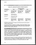 Section 403 Procedural and Monitoring Guidance
Viruses
Detecting viruses in marine waters requires collecting a representative water sample,
concentrating viruses in the sample, and identifying and estimating abundances of these
concentrated viruses. Difficulties in detecting virus abundances include:
• Viruses are very small (20-100 nm).
• Virus concentrations in waters are spatially and temporally variable, and
typically low.
• Dissolved and suspended material in the sample interferes with accurate
virus detection.
Because virus concentrations may be very low, significant volumes of water may be
required (e.g., on the order of tens to thousands of liters). Dose-response curves are
lacking for most pathogens; however, as few as 10 to 100 bacteria are capable of
inducing disease (OTA, 1987).
Three different techniques for concentrating and enumerating viruses are presented in
Standard Methods (APHA, 1989):
• Adsorption to and elution from microporous filters;
• Aluminum hydroxide adsorption and precipitation; and
• Polyethylene glycol hydroextraction-dialysis.
The adsorption and elution technique pressure-filters viruses on microporous filters and
then elutes them from the filter in a small liquid volume. Generally, two types of filters
are available: electronegative and electropositive filters. Currently, insufficient
documentation on the efficacy of electropositive filters exists. Limitations of this
technique include:
• The adsorbent filter may be clogged by suspended material.
• Dissolved colloid material may interfere by competing with viruses for
adsorption sites on the filter.
• Viruses adsorbed to suspended material may be removed during suspended
material clean-up procedures.
199
image:
Section 403 Procedural and Monitoring Guidance
Viruses
Detecting viruses in marine waters requires collecting a representative water sample,
concentrating viruses in the sample, and identifying and estimating abundances of these
concentrated viruses. Difficulties in detecting virus abundances include:
• Viruses are very small (20-100 nm).
• Virus concentrations in waters are spatially and temporally variable, and
typically low.
• Dissolved and suspended material in the sample interferes with accurate
virus detection.
Because virus concentrations may be very low, significant volumes of water may be
required (e.g., on the order of tens to thousands of liters). Dose-response curves are
lacking for most pathogens; however, as few as 10 to 100 bacteria are capable of
inducing disease (OTA, 1987).
Three different techniques for concentrating and enumerating viruses are presented in
Standard Methods (APHA, 1989):
• Adsorption to and elution from microporous filters;
• Aluminum hydroxide adsorption and precipitation; and
• Polyethylene glycol hydroextraction-dialysis.
The adsorption and elution technique pressure-filters viruses on microporous filters and
then elutes them from the filter in a small liquid volume. Generally, two types of filters
are available: electronegative and electropositive filters. Currently, insufficient
documentation on the efficacy of electropositive filters exists. Limitations of this
technique include:
• The adsorbent filter may be clogged by suspended material.
• Dissolved colloid material may interfere by competing with viruses for
adsorption sites on the filter.
• Viruses adsorbed to suspended material may be removed during suspended
material clean-up procedures.
199
image:
 Methods
 for recovering solids-associated viruses are found in APHA (1989). In spite of
these limitations, the adsorption and elution technique remains the most promising
method for detecting viruses.
Aluminum hydroxide adsorption and precipitation and polyethylene glycol
hydroextraction-dialysis are used to reconcentrate viruses in proteinaceous and organic
buffer eluates. These methods may be used to concentrate viruses in waters having
high virus densities (e.g., wastewaters). They may also be used as a second-step
concentration procedure following processing of large fluid volumes through
microporous filters. However, these two techniques are impractical for primary
processing of large fluid volumes (APHA, 1989).
New Techniques
Traditional techniques lack the ability to detect apparently viable, but nonculturable,
microorganisms. Recently developed monoclonal antibody and gene probe techniques
permit the detection and enumeration of both culturable and nonculturable
microorganisms. Since these methods have the ability to detect nonculturable
organisms, they may serve as more precise techniques for monitoring microbial water
quality. Furthermore, these new techniques will allow direct monitoring of pathogens of
concern. The goal of monitoring specific pathogens, such as Salmonella, Shigella,
Giardia, or Legionella, may soon be realized.
Sample Handling
Preservation and storage of water samples can be significant sources of error. Sample
bottles must be resistant to sterilization procedures. Samples should be refrigerated
(1-4°C) during transport to a laboratory and analyzed within 6 hours of collection
(USEPA, 1978).
4.11.4 QA/QC Considerations
It is recommended that sterile distilled water be transported to the field, transferred to a
sample bottle, and processed routinely as a field blank to ensure that samples were not
contaminated during collection and transport. It is also recommended that 10 percent of
the samples be analyzed in duplicate. Furthermore, 10 percent of the samples should
be split and analyzed by two or more laboratories.
Intralaboratory and interlaboratory quality control practices should be documented, and
QC reports should be available for inspection. Further recommended quality assurance
guidelines for a microbiology laboratory are available (Inhorn, 1977; Bordner et al.,
1978) and are also discussed in APHA (1989).
200
image:
Methods
Methods for recovering solids-associated viruses are found in APHA (1989). In spite of
these limitations, the adsorption and elution technique remains the most promising
method for detecting viruses.
Aluminum hydroxide adsorption and precipitation and polyethylene glycol
hydroextraction-dialysis are used to reconcentrate viruses in proteinaceous and organic
buffer eluates. These methods may be used to concentrate viruses in waters having
high virus densities (e.g., wastewaters). They may also be used as a second-step
concentration procedure following processing of large fluid volumes through
microporous filters. However, these two techniques are impractical for primary
processing of large fluid volumes (APHA, 1989).
New Techniques
Traditional techniques lack the ability to detect apparently viable, but nonculturable,
microorganisms. Recently developed monoclonal antibody and gene probe techniques
permit the detection and enumeration of both culturable and nonculturable
microorganisms. Since these methods have the ability to detect nonculturable
organisms, they may serve as more precise techniques for monitoring microbial water
quality. Furthermore, these new techniques will allow direct monitoring of pathogens of
concern. The goal of monitoring specific pathogens, such as Salmonella, Shigella,
Giardia, or Legionella, may soon be realized.
Sample Handling
Preservation and storage of water samples can be significant sources of error. Sample
bottles must be resistant to sterilization procedures. Samples should be refrigerated
(1-4°C) during transport to a laboratory and analyzed within 6 hours of collection
(USEPA, 1978).
4.11.4 QA/QC Considerations
It is recommended that sterile distilled water be transported to the field, transferred to a
sample bottle, and processed routinely as a field blank to ensure that samples were not
contaminated during collection and transport. It is also recommended that 10 percent of
the samples be analyzed in duplicate. Furthermore, 10 percent of the samples should
be split and analyzed by two or more laboratories.
Intralaboratory and interlaboratory quality control practices should be documented, and
QC reports should be available for inspection. Further recommended quality assurance
guidelines for a microbiology laboratory are available (Inhorn, 1977; Bordner et al.,
1978) and are also discussed in APHA (1989).
200
image:
 Section 403 Procedural and Monitoring Guidance
4.11.5 Statistical Design Considerations
Bacterial counts often are characterized as having a skewed distribution because of
many low values and a few high ones (APHA, 1989). Application of parametric
statistical techniques requires the assumption of symmetrical distributions such as the
normal curve. An approximate normal distribution can be obtained from positively
skewed data by converting numbers to their logarithms (APHA, 1989). Accordingly, the
preferred statistic for measuring central tendency of microbiological data is the
geometric mean.
Consideration of statistical strategies will mitigate the high costs of collecting and
processing samples. Power-cost analyses are necessary in selecting appropriate
sample/replicate number, sample location, and sampling frequency (Ferraro et al.,
1989).
4.11.6 Use of Data
The assessment of pathogen contamination should be a component of a monitoring
program where pathogens may present a risk to human health and the economic vitality
of an estuary. Monitoring of human pathogens provides information essential in relating
the temporal and spatial distribution of infectious agents in marine waters and shellfish
to the epidemiology of pathogens of concern (e.g., affected human populations,
locations, and timing of the outbreak).
Furthermore, monitoring data can be used to identify discharges that may be significant
sources of pathogens and to ensure that water quality standards are maintained.
Monitoring data can also be used to verify fate and transport, human health risk
assessment, and epidemiological modeling predictions.
4.11.7 Summary and Recommendations
Rationale
• The objective is to detect and describe spatial and temporal changes in
abundances of indicators of human health pathogens.
• Monitoring indicators of human pathogens provides information essential in
relating the presence of infectious agents in marine waters and shellfish to
the incidence of disease outbreaks and potential sources of these agents.
201
image:
Section 403 Procedural and Monitoring Guidance
4.11.5 Statistical Design Considerations
Bacterial counts often are characterized as having a skewed distribution because of
many low values and a few high ones (APHA, 1989). Application of parametric
statistical techniques requires the assumption of symmetrical distributions such as the
normal curve. An approximate normal distribution can be obtained from positively
skewed data by converting numbers to their logarithms (APHA, 1989). Accordingly, the
preferred statistic for measuring central tendency of microbiological data is the
geometric mean.
Consideration of statistical strategies will mitigate the high costs of collecting and
processing samples. Power-cost analyses are necessary in selecting appropriate
sample/replicate number, sample location, and sampling frequency (Ferraro et al.,
1989).
4.11.6 Use of Data
The assessment of pathogen contamination should be a component of a monitoring
program where pathogens may present a risk to human health and the economic vitality
of an estuary. Monitoring of human pathogens provides information essential in relating
the temporal and spatial distribution of infectious agents in marine waters and shellfish
to the epidemiology of pathogens of concern (e.g., affected human populations,
locations, and timing of the outbreak).
Furthermore, monitoring data can be used to identify discharges that may be significant
sources of pathogens and to ensure that water quality standards are maintained.
Monitoring data can also be used to verify fate and transport, human health risk
assessment, and epidemiological modeling predictions.
4.11.7 Summary and Recommendations
Rationale
• The objective is to detect and describe spatial and temporal changes in
abundances of indicators of human health pathogens.
• Monitoring indicators of human pathogens provides information essential in
relating the presence of infectious agents in marine waters and shellfish to
the incidence of disease outbreaks and potential sources of these agents.
201
image:
 Methods
Monitoring Design Considerations
• If feasible, samples of the surface microlayer should be collected separately
from samples of underlying waters. If not feasible, samples containing both
underlying and microlayer waters should be collected. It is highly
recommended that consistent types of sampling protocols be implemented to
allow for comparisons between studies.
• Analysis of tissues of sentinel organisms (e.g., mussels and oysters) confers
the following advantages:
- such organisms concentrate pathogens;
- such organisms provide a means of temporally integrating water quality
conditions; and
- such organisms may be deployed and maintained in a number of locales.
Analytical Methods Considerations
• Indicators of human pathogens should have the following characteristics:
- should be consistently found in high abundance in human fecal wastes;
- should not have significant extra-human fecal sources; and
- must provide temporally and spatially reliable and accurate appraisals of
the pathogen of concern.
• Fecal coliform bacteria densities.
- May not be a reliable indicator for predicting the risk associated with direct
exposures to pathogens.
- This measure provides a means to compare current data to historical data.
- Laboratory analyses include membrane filter and multiple-tube
fermentation techniques.
• Enterococci densities
- Densities are highly correlated with the incidence of gastrointestinal
symptoms.
- Taxonomic identifications are relatively simple and can reveal the kinds of
mammalian pollution.
- State-of-the-art genetic fingerprinting techniques can link bacteria in the
marine environment to specific sources; however, these techniques are
very costly and require further study to assess their reliability.
- Laboratory analyses include membrane filter technique.
• Virus densities
- Viruses are recognized as major etiologic agents for many outbreaks of
human illness.
202
image:
Methods
Monitoring Design Considerations
• If feasible, samples of the surface microlayer should be collected separately
from samples of underlying waters. If not feasible, samples containing both
underlying and microlayer waters should be collected. It is highly
recommended that consistent types of sampling protocols be implemented to
allow for comparisons between studies.
• Analysis of tissues of sentinel organisms (e.g., mussels and oysters) confers
the following advantages:
- such organisms concentrate pathogens;
- such organisms provide a means of temporally integrating water quality
conditions; and
- such organisms may be deployed and maintained in a number of locales.
Analytical Methods Considerations
• Indicators of human pathogens should have the following characteristics:
- should be consistently found in high abundance in human fecal wastes;
- should not have significant extra-human fecal sources; and
- must provide temporally and spatially reliable and accurate appraisals of
the pathogen of concern.
• Fecal coliform bacteria densities.
- May not be a reliable indicator for predicting the risk associated with direct
exposures to pathogens.
- This measure provides a means to compare current data to historical data.
- Laboratory analyses include membrane filter and multiple-tube
fermentation techniques.
• Enterococci densities
- Densities are highly correlated with the incidence of gastrointestinal
symptoms.
- Taxonomic identifications are relatively simple and can reveal the kinds of
mammalian pollution.
- State-of-the-art genetic fingerprinting techniques can link bacteria in the
marine environment to specific sources; however, these techniques are
very costly and require further study to assess their reliability.
- Laboratory analyses include membrane filter technique.
• Virus densities
- Viruses are recognized as major etiologic agents for many outbreaks of
human illness.
202
image:
 Section 403 Procedural and Monitoring Guidance
- Examination of water samples for enteric viruses is not recommended
because of methodology limitations.
- Laboratory analyses include absorption to an elution from microporous
filters, aluminum hydroxide absorption-precipitation, and polyethylene
glycol hydroextraction-dialysis.
• Monoclonal antibodies and gene probes show promise in detecting and
enumerating both culturable and nonculturable microorganisms.
QA/QC Considerations
• Sterile distilled water should be transported and transferred to sample bottles
as field blanks to assess contamination during collection and transport.
• Ten percent of the samples should be analyzed in duplicate.
• Ten percent of the samples should be split and analyzed at two or more
laboratories.
Statistical Design Considerations
« The preferred statistic for measuring central tendency of microbiological data
is the geometric mean.
Use of Data
• Provide essential information to assess threats to human health;
• Establish temporal and spatial trends in pathogen densities and identify
potential relationships between the presence of the indicator and incidence of
human illness; and
• Provide information that can be used to verify fate and transport, human
health risk, and epidemiology models.
203
image:
Section 403 Procedural and Monitoring Guidance
- Examination of water samples for enteric viruses is not recommended
because of methodology limitations.
- Laboratory analyses include absorption to an elution from microporous
filters, aluminum hydroxide absorption-precipitation, and polyethylene
glycol hydroextraction-dialysis.
• Monoclonal antibodies and gene probes show promise in detecting and
enumerating both culturable and nonculturable microorganisms.
QA/QC Considerations
• Sterile distilled water should be transported and transferred to sample bottles
as field blanks to assess contamination during collection and transport.
• Ten percent of the samples should be analyzed in duplicate.
• Ten percent of the samples should be split and analyzed at two or more
laboratories.
Statistical Design Considerations
« The preferred statistic for measuring central tendency of microbiological data
is the geometric mean.
Use of Data
• Provide essential information to assess threats to human health;
• Establish temporal and spatial trends in pathogen densities and identify
potential relationships between the presence of the indicator and incidence of
human illness; and
• Provide information that can be used to verify fate and transport, human
health risk, and epidemiology models.
203
image:
 Methods
4.12 EFFLUENT CHARACTERIZATION
"End-of-pipe" effluent characterizations based on laboratory studies can be used to
predict biological impacts of an effluent prior to a discharge. The Technical Support
Document for Water Quality-based Toxics Control (USEPA, 1991c) presents (among
other things) an integrated approach for ensuring protection of aquatic life and human
health from impacts caused by the release of toxics to surface waters. For the
protection of aquatic life, the integrated strategy involves the use of three control
approaches: the chemical-specific control approach, the whole-effluent toxicity control
approach, and the biological criteria/bioassessment and biosurvey approach. For the
protection of human health, technical constraints do not yet allow for full reliance on an
integrated strategy, and thus primarily chemical-specific assessments and control
techniques should be employed. Table 4-30 contains a list of terms used in effluent
characterization.
Pollutant-specific criteria developed pursuant to CWA section 304(a)(1) present
scientific data and guidance on the environmental effects of pollutants that reflect the
latest EPA recommendations on acceptable limits for aquatic life and human health
protection. These limitations are generally developed from laboratory-derived,
biologically-based numeric water quality criteria adopted within a State's water quality
standards. Water quality criteria are adopted by a State for the protection of designated
uses of the receiving water. Criteria can be specific numeric limits or, in the absence of
specific numeric criteria for a chemical, biological, or physical parameter, can be based
on narrative criteria. EPA publishes chemical-specific water quality criteria that may
provide the basis on which States adopt their criteria (USEPA, 1986-1988). EPA has
published 25 chemical-specific saltwater aquatic life criteria (acute and chronic).
When an effluent's constituents are not completely known or when a complex mixture of
potentially additive, antagonistic, or synergistic toxic pollutants is discharged, a
whole-effluent toxicity limitation can be. implemented. The whole-effluent toxicity
limitation can also be appropriate when more than one discharger is located in a specific
area and the potential exists for effluent mixing and additive toxic effects, and when a
pollutant-specific evaluation is impractical because of a lack of information about the
toxic effects of a pollutant. Toxicity evaluations such as these can be used as part of
403 monitoring.
4.12.1 Rationale
Effluent characterization can be used in the CWA section 403 point source discharge
program to address the following evaluation criteria:
204
image:
Methods
4.12 EFFLUENT CHARACTERIZATION
"End-of-pipe" effluent characterizations based on laboratory studies can be used to
predict biological impacts of an effluent prior to a discharge. The Technical Support
Document for Water Quality-based Toxics Control (USEPA, 1991c) presents (among
other things) an integrated approach for ensuring protection of aquatic life and human
health from impacts caused by the release of toxics to surface waters. For the
protection of aquatic life, the integrated strategy involves the use of three control
approaches: the chemical-specific control approach, the whole-effluent toxicity control
approach, and the biological criteria/bioassessment and biosurvey approach. For the
protection of human health, technical constraints do not yet allow for full reliance on an
integrated strategy, and thus primarily chemical-specific assessments and control
techniques should be employed. Table 4-30 contains a list of terms used in effluent
characterization.
Pollutant-specific criteria developed pursuant to CWA section 304(a)(1) present
scientific data and guidance on the environmental effects of pollutants that reflect the
latest EPA recommendations on acceptable limits for aquatic life and human health
protection. These limitations are generally developed from laboratory-derived,
biologically-based numeric water quality criteria adopted within a State's water quality
standards. Water quality criteria are adopted by a State for the protection of designated
uses of the receiving water. Criteria can be specific numeric limits or, in the absence of
specific numeric criteria for a chemical, biological, or physical parameter, can be based
on narrative criteria. EPA publishes chemical-specific water quality criteria that may
provide the basis on which States adopt their criteria (USEPA, 1986-1988). EPA has
published 25 chemical-specific saltwater aquatic life criteria (acute and chronic).
When an effluent's constituents are not completely known or when a complex mixture of
potentially additive, antagonistic, or synergistic toxic pollutants is discharged, a
whole-effluent toxicity limitation can be. implemented. The whole-effluent toxicity
limitation can also be appropriate when more than one discharger is located in a specific
area and the potential exists for effluent mixing and additive toxic effects, and when a
pollutant-specific evaluation is impractical because of a lack of information about the
toxic effects of a pollutant. Toxicity evaluations such as these can be used as part of
403 monitoring.
4.12.1 Rationale
Effluent characterization can be used in the CWA section 403 point source discharge
program to address the following evaluation criteria:
204
image:
 Section 403 Procedural and Monitoring Guidance
Table 4-30. List of Terms Used with Effluent Characterization
Acute
Acute-to-chronic ratio
(ACR)
Chronic
Composite sample
Effective concentration
Grab samples
A stimulus severe enough to rapidly induce an effect; in aquatic toxicity tests,
an effect observed in 96 hours or less typically is considered acute. When
referring to aquatic toxicology or human health, an acute effect is not always
measured in terms of lethality.
The ratio of the acute toxicity of an effluent or a toxicant to its chronic toxicity.
ACR is used as a factor for estimating chronic toxicity on the basis of acute
toxicity data, or the reverse.
A stimulus that lingers or continues for a relatively long period of time, often
one-tenth of the life span or more. Chronic should be considered a relative
term depending on the life span of an organism. The measurement of a
chonic effect can be reduced growth, reduced reproduction, etc., in addition
to lethality.
A single effluent sample collected over a 24-hour period, on which only one
toxicity test is performed.
A point estimate of the toxicant concentration that would cause an
observable adverse effect (such as death, immobilization, or serious
incapacitation) in a given percentage of the test organisms.
Samples collected over a very short period of time and on a relatively
infrequent basis. A separate toxicity test must be performed on each grab
sample.
Lowest-Observed-Adverse- The lowest concentration of an effluent or toxicant that results in statistically
Effect Level (LOAEL) significant adverse health effects as observed in chronic or subchronic
human epidemiology studies or animal exposure.
No-Observed-Adverse-
Effect Level (NOAEL)
No-Observed-Effect
Concentration (NOEC)
Toxicity characterization
Whole-effluent toxicity
A tested dose of an effluent or a toxicant below which no adverse biological
effects are observed, as identified from chronic or subchronic human
epidemiology studies or animal exposure studies.
The highest tested concentration of an effluent or a toxicant at which no
adverse effects are observed on the aquatic test organisms at a specific time
of observation. Determined using hypothesis testing.
A determination of the specific chemicals responsible for effluent toxicity.
The aggregate toxic effect of an effluent (usually measured directly with a
toxicity test).
205
image:
Section 403 Procedural and Monitoring Guidance
Table 4-30. List of Terms Used with Effluent Characterization
Acute
Acute-to-chronic ratio
(ACR)
Chronic
Composite sample
Effective concentration
Grab samples
A stimulus severe enough to rapidly induce an effect; in aquatic toxicity tests,
an effect observed in 96 hours or less typically is considered acute. When
referring to aquatic toxicology or human health, an acute effect is not always
measured in terms of lethality.
The ratio of the acute toxicity of an effluent or a toxicant to its chronic toxicity.
ACR is used as a factor for estimating chronic toxicity on the basis of acute
toxicity data, or the reverse.
A stimulus that lingers or continues for a relatively long period of time, often
one-tenth of the life span or more. Chronic should be considered a relative
term depending on the life span of an organism. The measurement of a
chonic effect can be reduced growth, reduced reproduction, etc., in addition
to lethality.
A single effluent sample collected over a 24-hour period, on which only one
toxicity test is performed.
A point estimate of the toxicant concentration that would cause an
observable adverse effect (such as death, immobilization, or serious
incapacitation) in a given percentage of the test organisms.
Samples collected over a very short period of time and on a relatively
infrequent basis. A separate toxicity test must be performed on each grab
sample.
Lowest-Observed-Adverse- The lowest concentration of an effluent or toxicant that results in statistically
Effect Level (LOAEL) significant adverse health effects as observed in chronic or subchronic
human epidemiology studies or animal exposure.
No-Observed-Adverse-
Effect Level (NOAEL)
No-Observed-Effect
Concentration (NOEC)
Toxicity characterization
Whole-effluent toxicity
A tested dose of an effluent or a toxicant below which no adverse biological
effects are observed, as identified from chronic or subchronic human
epidemiology studies or animal exposure studies.
The highest tested concentration of an effluent or a toxicant at which no
adverse effects are observed on the aquatic test organisms at a specific time
of observation. Determined using hypothesis testing.
A determination of the specific chemicals responsible for effluent toxicity.
The aggregate toxic effect of an effluent (usually measured directly with a
toxicity test).
205
image:
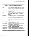 Methods
• The quantities, composition, and potential for bioaccumulation or persistence
of the pollutants to be discharged;
• The potential impact on human health through direct and indirect pathways; and
• Marine water quality criteria developed pursuant to section 304(a)(1).
Assessment of these evaluation criteria can be made through whole-effluent toxicity
testing (acute and chronic) and analysis of the chemical composition of the effluent.
This assessment would demonstrate potential impacts from the effluent in question.
4.12.2 Monitoring Design Considerations
Determination of whether an effluent sample is typical of the wastewater may require the
collection of a large number of samples. Further, what constitutes a "representative"
sample is a function of the parameter of concern. Guidelines for determining the
number and frequency of samples required to represent effluent quality are contained in
the Handbook for Sampling and Sample Preservation of Water and Wastewater
(USEPA, 1982b).
Both quantitative (change in concentration) and qualitative (change in toxicants)
variability commonly occur in effluents. Changes in effluent toxicity are the result of
varying concentrations of individual toxicants, different toxicants, changing in-stream
water quality characteristics (affecting compound toxicity), and analytical and
toxicological error. Conventional parameters, BOD, TSS, and other pollutants limited in
the facility's permit will provide an indication of the operational status of the treatment
system on the day of sampling. This information may be used in a determination as to
whether the system is operating properly, requires repair, or needs to be upgraded. For
industrial discharges, information on production levels and types of operating processes
may be helpful in determining the required magnitude of the monitoring program.
4.12.3 Analytical Methods Considerations
Sampling
The choice of grab or composite samples will depend on the specific discharge situation
(e.g., plant retention time) and the objectives of the test. In toxicity characterization
testing, samples that are very different from one another give results that are difficult to
interpret. However, composite sampling has an averaging effect, which tends to dilute
toxicity peaks and may thus provide misleading results when testing for acute toxicity.
Composited samples, therefore, are more appropriate for chronic toxicity tests where
peak toxicity of short duration is of less concern. If the toxicity of the effluent is variable,
grab samples collected during peaks of effluent toxicity provide a measure of maximum
effect. However, while grab sampling may provide information on maximum effluent
206
image:
Methods
• The quantities, composition, and potential for bioaccumulation or persistence
of the pollutants to be discharged;
• The potential impact on human health through direct and indirect pathways; and
• Marine water quality criteria developed pursuant to section 304(a)(1).
Assessment of these evaluation criteria can be made through whole-effluent toxicity
testing (acute and chronic) and analysis of the chemical composition of the effluent.
This assessment would demonstrate potential impacts from the effluent in question.
4.12.2 Monitoring Design Considerations
Determination of whether an effluent sample is typical of the wastewater may require the
collection of a large number of samples. Further, what constitutes a "representative"
sample is a function of the parameter of concern. Guidelines for determining the
number and frequency of samples required to represent effluent quality are contained in
the Handbook for Sampling and Sample Preservation of Water and Wastewater
(USEPA, 1982b).
Both quantitative (change in concentration) and qualitative (change in toxicants)
variability commonly occur in effluents. Changes in effluent toxicity are the result of
varying concentrations of individual toxicants, different toxicants, changing in-stream
water quality characteristics (affecting compound toxicity), and analytical and
toxicological error. Conventional parameters, BOD, TSS, and other pollutants limited in
the facility's permit will provide an indication of the operational status of the treatment
system on the day of sampling. This information may be used in a determination as to
whether the system is operating properly, requires repair, or needs to be upgraded. For
industrial discharges, information on production levels and types of operating processes
may be helpful in determining the required magnitude of the monitoring program.
4.12.3 Analytical Methods Considerations
Sampling
The choice of grab or composite samples will depend on the specific discharge situation
(e.g., plant retention time) and the objectives of the test. In toxicity characterization
testing, samples that are very different from one another give results that are difficult to
interpret. However, composite sampling has an averaging effect, which tends to dilute
toxicity peaks and may thus provide misleading results when testing for acute toxicity.
Composited samples, therefore, are more appropriate for chronic toxicity tests where
peak toxicity of short duration is of less concern. If the toxicity of the effluent is variable,
grab samples collected during peaks of effluent toxicity provide a measure of maximum
effect. However, while grab sampling may provide information on maximum effluent
206
image:
 Section 403 Procedural and Monitoring Guidance
toxicity, it can be difficult to schedule sampling to coincide with peaks in toxicity.
Aeration during collection and transfer of effluents should be minimized to reduce the
loss of volatile chemicals.
Chemical-Specific Analysis
Pollutant-specific testing for comparison to water quality criteria should be done
following standard methods. Choice of a particular method may vary depending on the
precision and accuracy required and the resources available for the study. A review of
water chemistry analytical methods is presented in the section in this report on water
quality and in Standard Methods for the Examination of Water and Wastewater (APHA,
1989). However, it should be noted that pollutant concentrations are considerably
higher in effluent streams and the precision required for adequate measurement is
lower.
Whole-Effluent Toxicity Analysis
Whole-effluent toxicity testing can be somewhat more complex than a pollutant-specific
approach. Upon arrival of the sample in the laboratory, temperature, pH, hardness, and
conductivity should be measured. Total residual chlorine, total ammonia, alkalinity,
dissolved oxygen (DO), and organic carbon measurements may also be appropriate.
These measurements can provide necessary information should the toxicity of the
effluent change over time.
EPA recommends that for whole-effluent toxicity data generation the process should be
divided into three basic steps: initial dilution determination, toxicity testing procedures,
and triggers for permit limit development. The dilution determination is an estimate of
the effluent dilution at the edge of the mixing zone and should take any applicable State
mixing zone requirements into consideration.
Whole-effluent toxicity testing should entail both acute and chronic testing. An acute
toxicity test is defined as a test of usually less than 96 hours in duration in which lethality
is the measured endpoint. A chronic toxicity test is defined as a long-term test in which
sublethal effects, such as fertilization, growth, and reproduction are usually measured,
although in highly toxic effluents lethality may also result. Traditionally, chronic tests are
full-life-cycle tests or at least 30-day tests. However, the duration of most of the EPA
chronic toxicity tests has been shortened to 7 days by focusing on the most sensitive
life-cycle stages. For this reason, the EPA chronic toxicity tests are called short-term
chronic tests. Whole-effluent toxicity limits can be inserted into permits as a means of
controlling pollutants when chemical-specific criteria have not been developed or
synergistic effects are found to occur.
207
image:
Section 403 Procedural and Monitoring Guidance
toxicity, it can be difficult to schedule sampling to coincide with peaks in toxicity.
Aeration during collection and transfer of effluents should be minimized to reduce the
loss of volatile chemicals.
Chemical-Specific Analysis
Pollutant-specific testing for comparison to water quality criteria should be done
following standard methods. Choice of a particular method may vary depending on the
precision and accuracy required and the resources available for the study. A review of
water chemistry analytical methods is presented in the section in this report on water
quality and in Standard Methods for the Examination of Water and Wastewater (APHA,
1989). However, it should be noted that pollutant concentrations are considerably
higher in effluent streams and the precision required for adequate measurement is
lower.
Whole-Effluent Toxicity Analysis
Whole-effluent toxicity testing can be somewhat more complex than a pollutant-specific
approach. Upon arrival of the sample in the laboratory, temperature, pH, hardness, and
conductivity should be measured. Total residual chlorine, total ammonia, alkalinity,
dissolved oxygen (DO), and organic carbon measurements may also be appropriate.
These measurements can provide necessary information should the toxicity of the
effluent change over time.
EPA recommends that for whole-effluent toxicity data generation the process should be
divided into three basic steps: initial dilution determination, toxicity testing procedures,
and triggers for permit limit development. The dilution determination is an estimate of
the effluent dilution at the edge of the mixing zone and should take any applicable State
mixing zone requirements into consideration.
Whole-effluent toxicity testing should entail both acute and chronic testing. An acute
toxicity test is defined as a test of usually less than 96 hours in duration in which lethality
is the measured endpoint. A chronic toxicity test is defined as a long-term test in which
sublethal effects, such as fertilization, growth, and reproduction are usually measured,
although in highly toxic effluents lethality may also result. Traditionally, chronic tests are
full-life-cycle tests or at least 30-day tests. However, the duration of most of the EPA
chronic toxicity tests has been shortened to 7 days by focusing on the most sensitive
life-cycle stages. For this reason, the EPA chronic toxicity tests are called short-term
chronic tests. Whole-effluent toxicity limits can be inserted into permits as a means of
controlling pollutants when chemical-specific criteria have not been developed or
synergistic effects are found to occur.
207
image:
 Methods
For whole-effluent toxicity testing, EPA recommends that three species (a vertebrate, an
invertebrate, and a plant) be tested quarterly for a minimum of 1 year. This may be
adjusted to require testing of only the most sensitive species. Conducting tests quarterly
for 1 year is recommended to adequately assess the variability of toxicity observed in
effluents. The use of three of the five commonly used marine organisms—inland
silverside, sheephead minnow, mysid shrimp, Champia, and sea urchin—has generally
been sufficient to measure the toxicity of any effluent for the purposes of projecting
effluent toxicity impact and making regulatory decisions. Specific test methodologies
can be found in a variety of EPA manuals, including Methods for Aquatic Toxicity
Identification Evaluations - Phases I, II, and III (USEPA, 1988a, b, c), Methods for
Measuring the Acute Toxicity of Effluents to Freshwater and Marine Organisms
(USEPA, 1985c), Short-Term Methods for Estimating the Chronic Toxicity of Effluents
and Receiving Waters to Marine and Estuarine Organisms (USEPA, 1988e), and
Biomonitoring for Control of Toxicity in Effluent Discharges to the Marine Environment
(USEPA, 1989b). Numerous other sources of toxicity testing methodologies exist (see
reference list) and may be more appropriate for the effluent of interest.
Biological Criteria/Bioassessment
To fully protect aquatic habitats, water quality criteria should address biological integrity.
Biocriteria should be used as a supplement to existing chemical-specific criteria and as
criteria where such chemical-specific criteria have not been established. Biocriteria are
numerical values or narrative expressions that describe the reference biological integrity
of aquatic communities inhabiting unimpaired waters. The biological communities in
these waters represent the best attainable conditions (USEPA, 1991c).
Resident biota integrate multiple impacts over time and can detect impairment from
known and unknown causes. Biocriteria can be used to verify improvement in water
quality in response to regulatory efforts and detect continuing degradation of waters.
Numeric criteria can provide effective monitoring criteria for inclusion in permits
(USEPA, 1991).
The assessment of biological integrity should include measures of the structure and
function of an aquatic community of species within a specified habitat. Expert
knowledge of the system is required for the selection of appropriate biological
components and measurements indices. See Section 4.5 for further discussion of
benthic community structure.
4.12.4 QA/QC Considerations
Basic sampling and laboratory quality assurance and quality control (QA/QC)
procedures for pollutant-specific characterization are addressed in the section on water
chemistry. QC problems specific to effluent characterization include variability in effluent
concentrations and toxicity response of test organisms, and changes in effluent toxicity
208
image:
Methods
For whole-effluent toxicity testing, EPA recommends that three species (a vertebrate, an
invertebrate, and a plant) be tested quarterly for a minimum of 1 year. This may be
adjusted to require testing of only the most sensitive species. Conducting tests quarterly
for 1 year is recommended to adequately assess the variability of toxicity observed in
effluents. The use of three of the five commonly used marine organisms—inland
silverside, sheephead minnow, mysid shrimp, Champia, and sea urchin—has generally
been sufficient to measure the toxicity of any effluent for the purposes of projecting
effluent toxicity impact and making regulatory decisions. Specific test methodologies
can be found in a variety of EPA manuals, including Methods for Aquatic Toxicity
Identification Evaluations - Phases I, II, and III (USEPA, 1988a, b, c), Methods for
Measuring the Acute Toxicity of Effluents to Freshwater and Marine Organisms
(USEPA, 1985c), Short-Term Methods for Estimating the Chronic Toxicity of Effluents
and Receiving Waters to Marine and Estuarine Organisms (USEPA, 1988e), and
Biomonitoring for Control of Toxicity in Effluent Discharges to the Marine Environment
(USEPA, 1989b). Numerous other sources of toxicity testing methodologies exist (see
reference list) and may be more appropriate for the effluent of interest.
Biological Criteria/Bioassessment
To fully protect aquatic habitats, water quality criteria should address biological integrity.
Biocriteria should be used as a supplement to existing chemical-specific criteria and as
criteria where such chemical-specific criteria have not been established. Biocriteria are
numerical values or narrative expressions that describe the reference biological integrity
of aquatic communities inhabiting unimpaired waters. The biological communities in
these waters represent the best attainable conditions (USEPA, 1991c).
Resident biota integrate multiple impacts over time and can detect impairment from
known and unknown causes. Biocriteria can be used to verify improvement in water
quality in response to regulatory efforts and detect continuing degradation of waters.
Numeric criteria can provide effective monitoring criteria for inclusion in permits
(USEPA, 1991).
The assessment of biological integrity should include measures of the structure and
function of an aquatic community of species within a specified habitat. Expert
knowledge of the system is required for the selection of appropriate biological
components and measurements indices. See Section 4.5 for further discussion of
benthic community structure.
4.12.4 QA/QC Considerations
Basic sampling and laboratory quality assurance and quality control (QA/QC)
procedures for pollutant-specific characterization are addressed in the section on water
chemistry. QC problems specific to effluent characterization include variability in effluent
concentrations and toxicity response of test organisms, and changes in effluent toxicity
208
image:
 Section 403 Procedural and Monitoring Guidance
over time. A quality assurance project plan (QAPj'P) should be developed and adhered
to. The QAPjP should include quality verification, which entails a demonstration that the
proposed study plan was followed as detailed and that work carried out was properly
documented. The QAPjP should increase communication between clients, program
planners, field and laboratory personnel, and data analysts. The QAPj'P must make
clear the specific responsibilities of each individual. The QC procedures involve
standardized guidelines, such as the number of samples to be taken and the mode of
collection, standard operating procedures for analyses, and spiking protocols. QC
protocols for standard toxicity test methods are described in USEPA (1985c).
4.12.5 Statistical Design Considerations
Statistical design of an effluent characterization project must account for variability in
effluent and toxicity testing response. However, the design of any given experiment
must be weighed against the importance of the data and decisions to be based on the
data. The critical nature of certain data will demand stringent controls, while statistical
rigor (and associated costs) can be lessened in other experiments having less impact
(e.g., initial toxicity testing).
The choice of a statistical method to analyze toxicity test data and the interpretation of
the results of the analysis of the data from toxicity tests can be problematic because of
the inherent variability and sometimes unavoidable anomalies in biological data. The
assistance of a trained statistician is recommended before selecting the method of
analysis and interpretation of the results. The data should be plotted to help detect
problems and unsuspected trends or patterns in the responses and to aid in
interpretation of the results. The analysis of the data is dependent upon the number of
replicates and the distribution and homogeneity of the data. A variety of statistical
methods for the analysis of toxicity data (including Dunnett's procedure, Bonferroni's
t-test, Steel's many-one rank test, the Wilcoson Rank Sum test, and the Probit analysis)
are presented in USEPA (1988e).
4.12.6 Use of Data
Pollutant-specific effluent characterization can be used for comparison to State water
quality standards. A chronic criterion is a level at which aquatic organisms and their
uses should not be affected unacceptably if the 4-day average concentration of the
pollutant is not exceeded more than once every 3 years on average. An acute criterion
is a limit at which the pollutant concentration should not be exceeded more than once
every 3 years on average. Care should be taken when applying these criteria to assess
potential impacts on locally important species that are very sensitive.
Whole-effluent toxicity testing data (both acute and chronic) may be used to screen an
effluent for potential unreasonable degradation of the environment. Whole-effluent
toxicity is a useful parameter for assessing and protecting against impacts on water
209
image:
Section 403 Procedural and Monitoring Guidance
over time. A quality assurance project plan (QAPj'P) should be developed and adhered
to. The QAPjP should include quality verification, which entails a demonstration that the
proposed study plan was followed as detailed and that work carried out was properly
documented. The QAPjP should increase communication between clients, program
planners, field and laboratory personnel, and data analysts. The QAPj'P must make
clear the specific responsibilities of each individual. The QC procedures involve
standardized guidelines, such as the number of samples to be taken and the mode of
collection, standard operating procedures for analyses, and spiking protocols. QC
protocols for standard toxicity test methods are described in USEPA (1985c).
4.12.5 Statistical Design Considerations
Statistical design of an effluent characterization project must account for variability in
effluent and toxicity testing response. However, the design of any given experiment
must be weighed against the importance of the data and decisions to be based on the
data. The critical nature of certain data will demand stringent controls, while statistical
rigor (and associated costs) can be lessened in other experiments having less impact
(e.g., initial toxicity testing).
The choice of a statistical method to analyze toxicity test data and the interpretation of
the results of the analysis of the data from toxicity tests can be problematic because of
the inherent variability and sometimes unavoidable anomalies in biological data. The
assistance of a trained statistician is recommended before selecting the method of
analysis and interpretation of the results. The data should be plotted to help detect
problems and unsuspected trends or patterns in the responses and to aid in
interpretation of the results. The analysis of the data is dependent upon the number of
replicates and the distribution and homogeneity of the data. A variety of statistical
methods for the analysis of toxicity data (including Dunnett's procedure, Bonferroni's
t-test, Steel's many-one rank test, the Wilcoson Rank Sum test, and the Probit analysis)
are presented in USEPA (1988e).
4.12.6 Use of Data
Pollutant-specific effluent characterization can be used for comparison to State water
quality standards. A chronic criterion is a level at which aquatic organisms and their
uses should not be affected unacceptably if the 4-day average concentration of the
pollutant is not exceeded more than once every 3 years on average. An acute criterion
is a limit at which the pollutant concentration should not be exceeded more than once
every 3 years on average. Care should be taken when applying these criteria to assess
potential impacts on locally important species that are very sensitive.
Whole-effluent toxicity testing data (both acute and chronic) may be used to screen an
effluent for potential unreasonable degradation of the environment. Whole-effluent
toxicity is a useful parameter for assessing and protecting against impacts on water
209
image:
 Methods
quality and designated uses caused by the aggregate toxic effect of the discharge.
Thus, toxicity itself is used as the effluent parameter, and the toxicants creating the
toxicity need not be specifically identified or controlled unless a Toxicity Reduction
Evaluation (TRE) is required to ensure compliance with a toxicity limit in the permit.
If a threshold of toxicity is desired, then the results of whole-effluent toxicity testing may
be used to derive the No-Observed-Effect Concentration (NOEC) and the
Lowest-Observed-Effect Concentration (LOEC). Whole-effluent toxicity testing can also
produce a concentration-dependent result of some amount of adverse effect called the
Effective Concentration (EC). For example, ECso is the effluent concentration that
would affect 50 percent of the organisms tested. Interpretation of EC values, therefore,
requires the judgment of a toxicologist.
4.12.7 Summary and Recommendations
Rationale
• Effluent characterization may be used to assess potential impacts, both acute
and chronic, of the effluent on the surrounding biological communities without
interference from other sources.
Monitoring Design Considerations
• Effluent variability, including potential changes in contaminants and
contaminant concentrations, should be considered when designing a
monitoring plan.
Analytical Methods Considerations
• Grab or composite samples should be used depending on the objectives and
type of test performed.
• Chemical-specific testing can be performed to characterize toxicity and
ensure compliance with water-quality standards.
• Both acute and chronic tests can be used to assess whole-effluent toxicity.
QA/QC Considerations
• See section on water chemistry.
• QAPjP should be developed, adhered to, and documented.
210
image:
Methods
quality and designated uses caused by the aggregate toxic effect of the discharge.
Thus, toxicity itself is used as the effluent parameter, and the toxicants creating the
toxicity need not be specifically identified or controlled unless a Toxicity Reduction
Evaluation (TRE) is required to ensure compliance with a toxicity limit in the permit.
If a threshold of toxicity is desired, then the results of whole-effluent toxicity testing may
be used to derive the No-Observed-Effect Concentration (NOEC) and the
Lowest-Observed-Effect Concentration (LOEC). Whole-effluent toxicity testing can also
produce a concentration-dependent result of some amount of adverse effect called the
Effective Concentration (EC). For example, ECso is the effluent concentration that
would affect 50 percent of the organisms tested. Interpretation of EC values, therefore,
requires the judgment of a toxicologist.
4.12.7 Summary and Recommendations
Rationale
• Effluent characterization may be used to assess potential impacts, both acute
and chronic, of the effluent on the surrounding biological communities without
interference from other sources.
Monitoring Design Considerations
• Effluent variability, including potential changes in contaminants and
contaminant concentrations, should be considered when designing a
monitoring plan.
Analytical Methods Considerations
• Grab or composite samples should be used depending on the objectives and
type of test performed.
• Chemical-specific testing can be performed to characterize toxicity and
ensure compliance with water-quality standards.
• Both acute and chronic tests can be used to assess whole-effluent toxicity.
QA/QC Considerations
• See section on water chemistry.
• QAPjP should be developed, adhered to, and documented.
210
image:
 Section 403 Procedural and Monitoring Guidance
Statistical Design Considerations
• Effluent variability and toxicity testing response must be accounted for in the
monitoring plan.
Use of Data
• Chronic and acute toxicity levels can be set in permits.
• Toxicity Reduction Evaluations (TREs) can be required.
• Threshold and effective concentrations can be established to predict
ecological risk.
211
image:
Section 403 Procedural and Monitoring Guidance
Statistical Design Considerations
• Effluent variability and toxicity testing response must be accounted for in the
monitoring plan.
Use of Data
• Chronic and acute toxicity levels can be set in permits.
• Toxicity Reduction Evaluations (TREs) can be required.
• Threshold and effective concentrations can be established to predict
ecological risk.
211
image:
 Methods
4.13 MESOCOSMS AND MICROCOSMS
The use of mesocosms and microcosms for the assessment of ecological impacts from
marine dischargers is considered to be premature. This monitoring approach is the
focus of research and holds promise for future use. It has been used to some extent by
EPA's Office of Pesticides to predict impacts from the use of pesticides.
Microcosms and mesocosms, on a small to medium size scale, respectively, attempt to
simulate the complex nature of natural environments. An effort is made to determine the
response of an ecosystem to perturbation through an accurate simulation of the
physical, chemical, and biological characteristics of an ecosystem and the biological
interactions of the organisms in the ecosystem. While there is no absolute separation
between a mesocosm and a microcosm, in practice most mesocosms are outdoors
where temperature and light intensity are ambient for the parent community. Most
mesocosm researchers try to realistically scale for the factors they think are most
important in controlling ecological relationships. Most microcosms are incubated in the
laboratory and are subject to greater environmental control. Microcosms are usually
smaller, and more replicates are used.
4.13.1 Rationale
Of the 10 guidelines used to determine unreasonable degradation or no irreparable
harm, several can be addressed through the use of mesocosms and microcosms
including:
• The potential transport of such pollutants by biological, physical or chemical
processes and
• The composition and vulnerability of potentially exposed biological
communities.
Mesocosms and microcosms can be used to gain a realistic characterization of
ecosystem-level impacts of marine discharges subject to section 403. With mesocosms
and microcosms, the responses of complete ecosystems to pollutants can be
investigated. Other advantages include the possibility of experimentation, at near
natural conditions, with addition of isotopic tracers to an ecosystem and the opportunity
to test numerical transport models under near natural conditions.
If insufficient information exists to determine whether a discharge will result in
unreasonable degradation of the marine environment, EPA must make a determination
as to whether a discharge will cause irreparable harm during the period in which
monitoring is undertaken. The use of microcosms allows for the incorporation of
ecosystem recovery (a critical factor in making a determination of irreparable harm) as
an endpoint for future ecological risk assessment (Perez et al., 1990).
212
image:
Methods
4.13 MESOCOSMS AND MICROCOSMS
The use of mesocosms and microcosms for the assessment of ecological impacts from
marine dischargers is considered to be premature. This monitoring approach is the
focus of research and holds promise for future use. It has been used to some extent by
EPA's Office of Pesticides to predict impacts from the use of pesticides.
Microcosms and mesocosms, on a small to medium size scale, respectively, attempt to
simulate the complex nature of natural environments. An effort is made to determine the
response of an ecosystem to perturbation through an accurate simulation of the
physical, chemical, and biological characteristics of an ecosystem and the biological
interactions of the organisms in the ecosystem. While there is no absolute separation
between a mesocosm and a microcosm, in practice most mesocosms are outdoors
where temperature and light intensity are ambient for the parent community. Most
mesocosm researchers try to realistically scale for the factors they think are most
important in controlling ecological relationships. Most microcosms are incubated in the
laboratory and are subject to greater environmental control. Microcosms are usually
smaller, and more replicates are used.
4.13.1 Rationale
Of the 10 guidelines used to determine unreasonable degradation or no irreparable
harm, several can be addressed through the use of mesocosms and microcosms
including:
• The potential transport of such pollutants by biological, physical or chemical
processes and
• The composition and vulnerability of potentially exposed biological
communities.
Mesocosms and microcosms can be used to gain a realistic characterization of
ecosystem-level impacts of marine discharges subject to section 403. With mesocosms
and microcosms, the responses of complete ecosystems to pollutants can be
investigated. Other advantages include the possibility of experimentation, at near
natural conditions, with addition of isotopic tracers to an ecosystem and the opportunity
to test numerical transport models under near natural conditions.
If insufficient information exists to determine whether a discharge will result in
unreasonable degradation of the marine environment, EPA must make a determination
as to whether a discharge will cause irreparable harm during the period in which
monitoring is undertaken. The use of microcosms allows for the incorporation of
ecosystem recovery (a critical factor in making a determination of irreparable harm) as
an endpoint for future ecological risk assessment (Perez et al., 1990).
212
image:
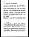 Section 403 Procedural and Monitoring Quittance
4.13.2 Monitoring Design Considerations
A microcosm should be designed to represent a miniature ecosystem that responds
quickly to perturbation. The emphasis is on ecosystem-level properties, although
species-level attributes such as fecundity and mortality can also be monitored if desired.
Most generic microcosms do not simulate a site-specific natural system, but function as
very generalized simulations of a large class of ecosystems. However, the use of
undisturbed, natural aquatic, and benthic communities (through the use of a sediment
core) in a single system allows for the simulation of a natural system (USEPA, 1983b).
The design of the microcosm allows the system to be defined in terms of its physical and
temporal boundaries, its light and temperature regime, its water composition, the
turbulence and turnover rate, the ratio of benthic surface area to seawater volume, the
sediment characteristics, and the water flow rate over the sediment surface.
The results of microcosm or mesocosm experiments are measured by the ecological
effects on the biota of the system. When selecting biota to include in the test, two
factors should be considered, both of which involve selection of the benthic component
of the system. If the natural system has more than one distinct benthic community, then
those organisms which are directly linked to human consumption or those which are
important to the economics and aesthetics of the area should be considered for
experimental use. Moreover, if some of the benthic communities contain species known
to be more sensitive to environmental contaminants than others, these communities
should also be considered.
4.13.3 Analytical Methods Considerations
Microcosms for which ecosystem effects protocols have been developed are small,
static, open ecosystems. Kenneth Perez and other researchers at the EPA
Environmental Research Laboratory in Narragansett, Rhode Island, developed an
experimental marine microcosm test protocol that employs a time frame of 30 days
(USEPA, 1983b). The methodology was published in the Federal Register (volume 52,
number 187, pages 36352-36360) for use in developing site-specific data on the
chemical fate and ecological effects of chemical substances subject to regulation under
the Toxic Substances Control Act (TSCA) and could be adapted to the 403 ocean
discharge program. This protocol attempts to couple undisturbed pelagic and benthic
communities within a single system, the physical and chemical conditions of which are
equated to those in the natural system being simulated. The protocol and support
document (USEPA, 1990e) describes the steps necessary to develop the experimental
microcosm (tanks, paddles, benthic cylinders, pumps, and pump air supply) and support
equipment (room, water bath, light and turbulence fixtures, test compartments, and an
air evacuation system). A diver-collected sediment core is used for the benthic
subsystem, and the test water is collected by a nondestructive method and exchanged
at least three times a week, coinciding with biological and chemical sample collection.
Water flow, turbulence, light intensity, temperature, and simulated tidal flow are all
controlled to simulate the natural system for the 30-day time period.
213
image:
Section 403 Procedural and Monitoring Quittance
4.13.2 Monitoring Design Considerations
A microcosm should be designed to represent a miniature ecosystem that responds
quickly to perturbation. The emphasis is on ecosystem-level properties, although
species-level attributes such as fecundity and mortality can also be monitored if desired.
Most generic microcosms do not simulate a site-specific natural system, but function as
very generalized simulations of a large class of ecosystems. However, the use of
undisturbed, natural aquatic, and benthic communities (through the use of a sediment
core) in a single system allows for the simulation of a natural system (USEPA, 1983b).
The design of the microcosm allows the system to be defined in terms of its physical and
temporal boundaries, its light and temperature regime, its water composition, the
turbulence and turnover rate, the ratio of benthic surface area to seawater volume, the
sediment characteristics, and the water flow rate over the sediment surface.
The results of microcosm or mesocosm experiments are measured by the ecological
effects on the biota of the system. When selecting biota to include in the test, two
factors should be considered, both of which involve selection of the benthic component
of the system. If the natural system has more than one distinct benthic community, then
those organisms which are directly linked to human consumption or those which are
important to the economics and aesthetics of the area should be considered for
experimental use. Moreover, if some of the benthic communities contain species known
to be more sensitive to environmental contaminants than others, these communities
should also be considered.
4.13.3 Analytical Methods Considerations
Microcosms for which ecosystem effects protocols have been developed are small,
static, open ecosystems. Kenneth Perez and other researchers at the EPA
Environmental Research Laboratory in Narragansett, Rhode Island, developed an
experimental marine microcosm test protocol that employs a time frame of 30 days
(USEPA, 1983b). The methodology was published in the Federal Register (volume 52,
number 187, pages 36352-36360) for use in developing site-specific data on the
chemical fate and ecological effects of chemical substances subject to regulation under
the Toxic Substances Control Act (TSCA) and could be adapted to the 403 ocean
discharge program. This protocol attempts to couple undisturbed pelagic and benthic
communities within a single system, the physical and chemical conditions of which are
equated to those in the natural system being simulated. The protocol and support
document (USEPA, 1990e) describes the steps necessary to develop the experimental
microcosm (tanks, paddles, benthic cylinders, pumps, and pump air supply) and support
equipment (room, water bath, light and turbulence fixtures, test compartments, and an
air evacuation system). A diver-collected sediment core is used for the benthic
subsystem, and the test water is collected by a nondestructive method and exchanged
at least three times a week, coinciding with biological and chemical sample collection.
Water flow, turbulence, light intensity, temperature, and simulated tidal flow are all
controlled to simulate the natural system for the 30-day time period.
213
image:
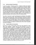 Methods
Other researchers contend that to study ecosystem-level effects it is essential that the
microcosms function (1) as homeostatic, self-sustaining ecosystems capable of existing
through at least a year and (2) independent of outside subsidies except for light and
replacement of evaporated water. Each microcosm is considered a unique ecosystem
and intraexperiment replication among microcosms is enhanced by using defined
chemical media and standard physical conditions (light, temperature, day length).
Inoculation with well-developed interactive couplings of the organisms is essential to
achieve these goals. Selection of the exact species to be used should be based on the
specific objectives of the study.
During microcosm studies, effluent to be tested should be added on a gradient. A
typical experimental design might consist of six replicates in each of four treatment
groups: a control, a single addition of a low concentration, a single addition of a high
concentration, and repeated additions of low concentrations. Example protocol steps
and the variables monitored for this type of generic microcosm are described in Taub
(1984).
The physical structure of a mesocosm system determines the ability of water,
organisms, and pollutants to move from compartment to compartment within the system.
Coastal ecosystems and the fate and effects of pollutants within these systems are
strongly affected by vertical mixing and the interaction of planktonic and benthic
processes. Donaghay (1984) classified mesocosm systems by their degree of
planktonic/benthic coupling into three categories: single well-mixed benthic coupled,
single stratified, and totally benthic decoupled. Single well-mixed benthic coupled
systems are composed of a well-mixed water column in direct contact with sediment and
benthos. This system has been used extensively at the Marine Ecosystem Research
Laboratory (MERL) with very good results validating field data; defining loadings, fates,
and effects; and manipulating natural systems to define underlying processes. The
single stratified system design involves well-mixed top and bottom layers separated by
an unmixed thermocline with only the bottom layer in contact with the sediment. The
system is used to study systems where stratification is important. The single system
without benthic coupling is intended to model fates and effects in stratified deep water
systems without benthic coupling.
4.13.4 QA/QC Considerations
In some cases the accuracy of the results of mesocosms and microcosms may be
limited by a number of factors. The size of the systems most often excludes
macrofauna such as fish and large crustaceans. The size of a microcosm can also
affect the mixing rates of surficial sediments. An increase in the size of a microcosm will
result in an increase in exposure of sediment particles to the overlying water column.
Results from smaller-sized systems have underestimated potential risks of complex
effluent (Perez et al., in press; Pontasch et al., 1989); however, attempts are being
214
image:
Methods
Other researchers contend that to study ecosystem-level effects it is essential that the
microcosms function (1) as homeostatic, self-sustaining ecosystems capable of existing
through at least a year and (2) independent of outside subsidies except for light and
replacement of evaporated water. Each microcosm is considered a unique ecosystem
and intraexperiment replication among microcosms is enhanced by using defined
chemical media and standard physical conditions (light, temperature, day length).
Inoculation with well-developed interactive couplings of the organisms is essential to
achieve these goals. Selection of the exact species to be used should be based on the
specific objectives of the study.
During microcosm studies, effluent to be tested should be added on a gradient. A
typical experimental design might consist of six replicates in each of four treatment
groups: a control, a single addition of a low concentration, a single addition of a high
concentration, and repeated additions of low concentrations. Example protocol steps
and the variables monitored for this type of generic microcosm are described in Taub
(1984).
The physical structure of a mesocosm system determines the ability of water,
organisms, and pollutants to move from compartment to compartment within the system.
Coastal ecosystems and the fate and effects of pollutants within these systems are
strongly affected by vertical mixing and the interaction of planktonic and benthic
processes. Donaghay (1984) classified mesocosm systems by their degree of
planktonic/benthic coupling into three categories: single well-mixed benthic coupled,
single stratified, and totally benthic decoupled. Single well-mixed benthic coupled
systems are composed of a well-mixed water column in direct contact with sediment and
benthos. This system has been used extensively at the Marine Ecosystem Research
Laboratory (MERL) with very good results validating field data; defining loadings, fates,
and effects; and manipulating natural systems to define underlying processes. The
single stratified system design involves well-mixed top and bottom layers separated by
an unmixed thermocline with only the bottom layer in contact with the sediment. The
system is used to study systems where stratification is important. The single system
without benthic coupling is intended to model fates and effects in stratified deep water
systems without benthic coupling.
4.13.4 QA/QC Considerations
In some cases the accuracy of the results of mesocosms and microcosms may be
limited by a number of factors. The size of the systems most often excludes
macrofauna such as fish and large crustaceans. The size of a microcosm can also
affect the mixing rates of surficial sediments. An increase in the size of a microcosm will
result in an increase in exposure of sediment particles to the overlying water column.
Results from smaller-sized systems have underestimated potential risks of complex
effluent (Perez et al., in press; Pontasch et al., 1989); however, attempts are being
214
image:
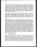 Section 403 Procedural and Monitoring Guidance
made to develop "scaling laws" to describe this relationship. These systems are also
limited to photo-stable test substances because the light intensity may be higher than
that which would occur naturally.
4.13.5 Statistical Design Considerations
The results of the microcosm and mesocosm experiments assist in determining the fates
and ecological effects of contaminants within a marine system. The pelagic biota are
characterized by the number and species composition of phytoplankton, zooplankton,
and transient larval forms. The benthic community is characterized by the structural
composition (see Section 4.5, Benthic Community Structure). The experimental marine
test protocol (USEPA, 1990e) recommended test design and statistical analysis allow for
the independent assessment of the solvent carrier (if used) and the effluent for all
variables measured. Also, the differences in the biotic response between the control
microcosms and the natural system will provide a measure of the validity of the test
response. A multivariate analysis of variance, followed by univariate analysis, and
regression techniques are recommended for the analysis of all data.
Statistical design considerations of mesocosms must consider that the scientific and
financial resources for mesocosm studies are limited. Therefore, efforts must be made
to maximize the information gained and the statistical rigor of the analysis while
minimizing the number of systems analyzed. Four different experimental designs are
presented by Donaghay (1984): single system, paired system, replicated, and single
gradient. Each design has advantages and disadvantages, and each is appropriate for
specific purposes.
4.13.6 Use of Data
Mesocosm research and microcosm research serve somewhat different purposes. If a
researcher wants to have maximum confidence in extrapolating back to a specific,
large-scale environment, the mesocosm provides greater realism in that it allows more
large-scale processes to be included in the system. If simplification is the goal—either
to semi-isolate certain components to determine their importance in the degradation of
pollutants or to provide more easily analyzed ecosystems for test purposes—then
microcosms are more appropriate.
The use of microcosms and/or mesocosms in an ocean discharge criteria evaluation as
mandated under section 403 would be most appropriate for general permits issued for a
whole category of discharges (e.g., regional oil and gas exploration/production activities)
mainly because of the higher cost associated with implementing a series of such
experiments. However, the use of microcosms and mesocosms can be less expensive
than implementing field experiments and can provide quantitative estimates of
processes and responses that can only be assessed qualitatively with field experiments.
In addition, Perez and Morrison (1985) showed that the monetary costs of environmental
215
image:
Section 403 Procedural and Monitoring Guidance
made to develop "scaling laws" to describe this relationship. These systems are also
limited to photo-stable test substances because the light intensity may be higher than
that which would occur naturally.
4.13.5 Statistical Design Considerations
The results of the microcosm and mesocosm experiments assist in determining the fates
and ecological effects of contaminants within a marine system. The pelagic biota are
characterized by the number and species composition of phytoplankton, zooplankton,
and transient larval forms. The benthic community is characterized by the structural
composition (see Section 4.5, Benthic Community Structure). The experimental marine
test protocol (USEPA, 1990e) recommended test design and statistical analysis allow for
the independent assessment of the solvent carrier (if used) and the effluent for all
variables measured. Also, the differences in the biotic response between the control
microcosms and the natural system will provide a measure of the validity of the test
response. A multivariate analysis of variance, followed by univariate analysis, and
regression techniques are recommended for the analysis of all data.
Statistical design considerations of mesocosms must consider that the scientific and
financial resources for mesocosm studies are limited. Therefore, efforts must be made
to maximize the information gained and the statistical rigor of the analysis while
minimizing the number of systems analyzed. Four different experimental designs are
presented by Donaghay (1984): single system, paired system, replicated, and single
gradient. Each design has advantages and disadvantages, and each is appropriate for
specific purposes.
4.13.6 Use of Data
Mesocosm research and microcosm research serve somewhat different purposes. If a
researcher wants to have maximum confidence in extrapolating back to a specific,
large-scale environment, the mesocosm provides greater realism in that it allows more
large-scale processes to be included in the system. If simplification is the goal—either
to semi-isolate certain components to determine their importance in the degradation of
pollutants or to provide more easily analyzed ecosystems for test purposes—then
microcosms are more appropriate.
The use of microcosms and/or mesocosms in an ocean discharge criteria evaluation as
mandated under section 403 would be most appropriate for general permits issued for a
whole category of discharges (e.g., regional oil and gas exploration/production activities)
mainly because of the higher cost associated with implementing a series of such
experiments. However, the use of microcosms and mesocosms can be less expensive
than implementing field experiments and can provide quantitative estimates of
processes and responses that can only be assessed qualitatively with field experiments.
In addition, Perez and Morrison (1985) showed that the monetary costs of environmental
215
image:
 Methods
assessments of a single chemical using a single microcosm system versus a series of
simple bioassay and physicochemical test systems are, at the worst case, effectively
equivalent. Assessments of complex effluents performed using microcosms could result
in more accurate results with a potential cost savings.
The use of microcosms and/or mesocosms could add significant benefits to an
ecological risk assessment of an ocean discharge. Microcosms and/or mesocosms can
be used to estimate ecological effects, chemical fate, transport mechanisms,
bioaccumulation, and ecological risk. Where multiple discharges occur in one area,
microcosms and/or mesocosms could be used to assess the risk associated with
individual discharges or combinations of discharges. Estimating ecosystem recovery
through the use of mesocosms in ecological risk assessments is a recent application
(Perez et al., 1990) and could provide important information concerning the occurrence
of irreparable harm.
4.13.7 Summary and Recommendations
Rationale
• Mesocosms and microcosms can be used to gain a realistic characterization
of ecosystem-level impacts of marine discharges subject to section 403(c).
• The transport and fate of pollutants to the complete ecosystems can be
investigated in near natural conditions.
Monitoring Design Considerations
• A microcosm should be designed to represent a miniature ecosystem that
responds quickly to perturbation.
• Most generic microcosms do not simulate a site-specific natural system, but
function as very generalized simulations of a large class of ecosystems.
• The design of the microcosm allows the system to be defined in terms of its
physical and temporal boundaries, its light and temperature regime, its water
composition, the turbulence and turnover rate, the ratio of benthic surface
area to seawater volume, the sediment characteristics, and the water flow
rate over the sediment surface.
• The results of microcosm or mesocosm experiments are measured by the
ecological effects on the biota of the system.
• Microcosm studies have been designed for 30 days to more than a year in
duration.
216
image:
Methods
assessments of a single chemical using a single microcosm system versus a series of
simple bioassay and physicochemical test systems are, at the worst case, effectively
equivalent. Assessments of complex effluents performed using microcosms could result
in more accurate results with a potential cost savings.
The use of microcosms and/or mesocosms could add significant benefits to an
ecological risk assessment of an ocean discharge. Microcosms and/or mesocosms can
be used to estimate ecological effects, chemical fate, transport mechanisms,
bioaccumulation, and ecological risk. Where multiple discharges occur in one area,
microcosms and/or mesocosms could be used to assess the risk associated with
individual discharges or combinations of discharges. Estimating ecosystem recovery
through the use of mesocosms in ecological risk assessments is a recent application
(Perez et al., 1990) and could provide important information concerning the occurrence
of irreparable harm.
4.13.7 Summary and Recommendations
Rationale
• Mesocosms and microcosms can be used to gain a realistic characterization
of ecosystem-level impacts of marine discharges subject to section 403(c).
• The transport and fate of pollutants to the complete ecosystems can be
investigated in near natural conditions.
Monitoring Design Considerations
• A microcosm should be designed to represent a miniature ecosystem that
responds quickly to perturbation.
• Most generic microcosms do not simulate a site-specific natural system, but
function as very generalized simulations of a large class of ecosystems.
• The design of the microcosm allows the system to be defined in terms of its
physical and temporal boundaries, its light and temperature regime, its water
composition, the turbulence and turnover rate, the ratio of benthic surface
area to seawater volume, the sediment characteristics, and the water flow
rate over the sediment surface.
• The results of microcosm or mesocosm experiments are measured by the
ecological effects on the biota of the system.
• Microcosm studies have been designed for 30 days to more than a year in
duration.
216
image:
 Section 403 Procedural and Monitoring Guidance
Analytical Method
• During microcosm studies, effluent to be tested should be added on a
gradient. A typical experimental design might consist of six replicates in each
of four treatment groups: a control, a single addition of a low concentration, a
single addition of a high concentration, and repeated additions of low
concentrations.
• Mesocosm systems can be classified by their degree of planktonic/benthic
coupling into single, well-mixed benthic coupled; single stratified; and totally
benthic decoupled systems.
QA/QC Analysis
• The results of microcosm and mesocosm studies are limited by the size of
the system.
• Scaling laws may be used to translate from microcosms to full-scale
ecosystems.
Statistical Design Considerations
• A multivariate analysis of variance, followed by univariate analysis, and
regression techniques are recommended for the analysis of all data.
• Efforts must be made to maximize the information gained and the statistical
rigor of the analysis while minimizing the number of systems analyzed.
Use of Data
• Data can be used to estimate ecological effects, chemical fate, transport
mechanisms, bioaccumulation, and ecological risks.
• Data can also be used to assess impacts of individual or multiple discharges
and to estimate recovery time.
• Mesocosms are most appropriate for use when maximum confidence in
extrapolating back to a specific, large-scale environment is desired.
• Microcosms are most appropriate for use when simplification is the goal,
either to isolate certain components to determine their importance or to
provide more easily analyzed ecosystems for test purposes.
• Microcosms and rnesocosms may be most appropriate for use for general
permits issued for a whole category of discharges.
• There can be cost advantages to using microcosms and rnesocosms under
certain circumstances.
217
image:
Section 403 Procedural and Monitoring Guidance
Analytical Method
• During microcosm studies, effluent to be tested should be added on a
gradient. A typical experimental design might consist of six replicates in each
of four treatment groups: a control, a single addition of a low concentration, a
single addition of a high concentration, and repeated additions of low
concentrations.
• Mesocosm systems can be classified by their degree of planktonic/benthic
coupling into single, well-mixed benthic coupled; single stratified; and totally
benthic decoupled systems.
QA/QC Analysis
• The results of microcosm and mesocosm studies are limited by the size of
the system.
• Scaling laws may be used to translate from microcosms to full-scale
ecosystems.
Statistical Design Considerations
• A multivariate analysis of variance, followed by univariate analysis, and
regression techniques are recommended for the analysis of all data.
• Efforts must be made to maximize the information gained and the statistical
rigor of the analysis while minimizing the number of systems analyzed.
Use of Data
• Data can be used to estimate ecological effects, chemical fate, transport
mechanisms, bioaccumulation, and ecological risks.
• Data can also be used to assess impacts of individual or multiple discharges
and to estimate recovery time.
• Mesocosms are most appropriate for use when maximum confidence in
extrapolating back to a specific, large-scale environment is desired.
• Microcosms are most appropriate for use when simplification is the goal,
either to isolate certain components to determine their importance or to
provide more easily analyzed ecosystems for test purposes.
• Microcosms and rnesocosms may be most appropriate for use for general
permits issued for a whole category of discharges.
• There can be cost advantages to using microcosms and rnesocosms under
certain circumstances.
217
image:
 image:
 5. LITERATURE CITED
Adamus, P.R., E.J. Clairain, Jr., D.R. Smith, and R.E. Young. 1987. Wetland
evaluation technique (WET). Vol. II. Technical report Y-87. U.S. Army Corps of
Engineers, Waterways Experiment Station, Vicksburg, MS.
Anderberg, M. R. 1973. Cluster analysis for applications. Academic Press, New York,
NY.
Anderson, D. 1990. Immunological indicators: Effects of environmental stress on
immune protection and disease outbreaks. Proceedings American Fisheries Society
Symposium 8: 38-50, Washington, DC.
Anderson, D., O. Dixon, arid E. Lizzio. 1986. Immunization and culture of Rainbow
Trout organ sections in vitro. Vet. Immunol. Immun. 12: 203-211.
Anderson, R.S. 1987. Immunocompetence in invertebrates. In Pollutant studies in
marine animals, ed. C. S. Giam and L. E. Ray. CRC Press, Boca Raton, FL.
Anderson, R.S. 1990. Effects of pollutant exposure on bactericidal activity of
Mercenaria mercenaria hemolymph. In Biological markers of environmental
contaminants, ed. J.F. McCarthy and L.R. Shugart. American Chemical Society, Los
Angeles, CA.
APHA. 1989. American Public Health Association, American Water Works Association,
and Water Pollution Control Federation. Standard methods for the examination of water
and wastewater. 17th ed. American Public Health Association, Washington, DC.
Appell, G.F., and T.B. Curtin. 1990. Proceedings of the IEEE Fourth Working
Conference on Current Measurement. Institute of Electrical and Electronic Engineers,
New York, NY.
Appell, G.F., and W.E. Woodward. 1986. Proceedings of the IEEE Third Working
Conference on Current Measurement. Institute of Electrical and Electronic Engineers,
New York, NY.
Armstrong, N.E., P.N. Storrs, and H.F. Ludwig. 1970. Ecosystem-pollution interactions
in San Francisco Bay. J. Water Poll. Control Fed.
219
image:
5. LITERATURE CITED
Adamus, P.R., E.J. Clairain, Jr., D.R. Smith, and R.E. Young. 1987. Wetland
evaluation technique (WET). Vol. II. Technical report Y-87. U.S. Army Corps of
Engineers, Waterways Experiment Station, Vicksburg, MS.
Anderberg, M. R. 1973. Cluster analysis for applications. Academic Press, New York,
NY.
Anderson, D. 1990. Immunological indicators: Effects of environmental stress on
immune protection and disease outbreaks. Proceedings American Fisheries Society
Symposium 8: 38-50, Washington, DC.
Anderson, D., O. Dixon, arid E. Lizzio. 1986. Immunization and culture of Rainbow
Trout organ sections in vitro. Vet. Immunol. Immun. 12: 203-211.
Anderson, R.S. 1987. Immunocompetence in invertebrates. In Pollutant studies in
marine animals, ed. C. S. Giam and L. E. Ray. CRC Press, Boca Raton, FL.
Anderson, R.S. 1990. Effects of pollutant exposure on bactericidal activity of
Mercenaria mercenaria hemolymph. In Biological markers of environmental
contaminants, ed. J.F. McCarthy and L.R. Shugart. American Chemical Society, Los
Angeles, CA.
APHA. 1989. American Public Health Association, American Water Works Association,
and Water Pollution Control Federation. Standard methods for the examination of water
and wastewater. 17th ed. American Public Health Association, Washington, DC.
Appell, G.F., and T.B. Curtin. 1990. Proceedings of the IEEE Fourth Working
Conference on Current Measurement. Institute of Electrical and Electronic Engineers,
New York, NY.
Appell, G.F., and W.E. Woodward. 1986. Proceedings of the IEEE Third Working
Conference on Current Measurement. Institute of Electrical and Electronic Engineers,
New York, NY.
Armstrong, N.E., P.N. Storrs, and H.F. Ludwig. 1970. Ecosystem-pollution interactions
in San Francisco Bay. J. Water Poll. Control Fed.
219
image:
 Literature Cited
ASTM. 1990. Standard guide for conducting 10-day static sediment toxicity tests with
marine and estuarine amphipods. Guide E1367-90. American Society for Testing and
Materials, Philadelphia, PA.
ASTM. 1991. Standard guide for collection, storage, characterization, and manipulation
of sediments for toxicological testing. ASTM Designation E1391-90. In Annual book of
ASTM standards. American Society for Testing and Materials, Philadelphia, PA.
Azam, F., T. Fenchel, J.G. Field, J.S. Gray, L.A. Meyer-Reil, and F. Thingstad. 1983.
The ecological role of water column microbes in the sea. Mar. Ecol. Prog. Ser.
10:257-263.
Bechtel, T.J., and BJ. Copeland. 1970. Fish species diversity indices as indicators of
pollution in Galveston Bay, Texas. Contrib. in Mar. Sci. 15:103-132.
Becker, D.S., and J. W. Armstrong. 1988. Development of regionally standardized
protocols for marine environmental studies. Mar. Pollut. Bull. 19(7):310-313.
Beers, J.R., G.L. Stewart, and J.D.H. Strickland. 1967. A pumping system for sampling
small plankton. J. Fish. Res. Board Can. 24:1811-1818.
Beukema, JJ. 1988. An evaluation of the ABC method (abundance-biomass
comparison) as applied to macrozoobenthic communities living on tidal flats in the Dutch
Wadden Sea. Mar. Biol. 99: 425-433.
Bilyard, G.R. 1987. The value of benthic infauna in marine pollution monitoring studies.
Mar. Poll. Bull. 18: 581-585.
Bisson, J.W., and V.J. Cabelli. 1979. Membrane filtration enumeration method for
Clostridium perfringens. Appl. Environ. Microbiol. 37: 55-66.
Blaxhall, P., and K. Daisley. 1973. Routine haematological methods for use with fish
blood. J. Fish Biol. 5: 771.
Boehm, P.O. 1984. The Status and Trends Program: Recommendations for design and
implementation of the chemical measurement segment. Workshop report. NOAA,
Rockville, MD.
Boesch, D. F. 1977. Application of numerical classification in ecological investigations
of water pollution. EPA 600/3-77-033. U.S. Environmental Protection Agency, Office of
Research and Development, Corvallis, OR.
220
image:
Literature Cited
ASTM. 1990. Standard guide for conducting 10-day static sediment toxicity tests with
marine and estuarine amphipods. Guide E1367-90. American Society for Testing and
Materials, Philadelphia, PA.
ASTM. 1991. Standard guide for collection, storage, characterization, and manipulation
of sediments for toxicological testing. ASTM Designation E1391-90. In Annual book of
ASTM standards. American Society for Testing and Materials, Philadelphia, PA.
Azam, F., T. Fenchel, J.G. Field, J.S. Gray, L.A. Meyer-Reil, and F. Thingstad. 1983.
The ecological role of water column microbes in the sea. Mar. Ecol. Prog. Ser.
10:257-263.
Bechtel, T.J., and BJ. Copeland. 1970. Fish species diversity indices as indicators of
pollution in Galveston Bay, Texas. Contrib. in Mar. Sci. 15:103-132.
Becker, D.S., and J. W. Armstrong. 1988. Development of regionally standardized
protocols for marine environmental studies. Mar. Pollut. Bull. 19(7):310-313.
Beers, J.R., G.L. Stewart, and J.D.H. Strickland. 1967. A pumping system for sampling
small plankton. J. Fish. Res. Board Can. 24:1811-1818.
Beukema, JJ. 1988. An evaluation of the ABC method (abundance-biomass
comparison) as applied to macrozoobenthic communities living on tidal flats in the Dutch
Wadden Sea. Mar. Biol. 99: 425-433.
Bilyard, G.R. 1987. The value of benthic infauna in marine pollution monitoring studies.
Mar. Poll. Bull. 18: 581-585.
Bisson, J.W., and V.J. Cabelli. 1979. Membrane filtration enumeration method for
Clostridium perfringens. Appl. Environ. Microbiol. 37: 55-66.
Blaxhall, P., and K. Daisley. 1973. Routine haematological methods for use with fish
blood. J. Fish Biol. 5: 771.
Boehm, P.O. 1984. The Status and Trends Program: Recommendations for design and
implementation of the chemical measurement segment. Workshop report. NOAA,
Rockville, MD.
Boesch, D. F. 1977. Application of numerical classification in ecological investigations
of water pollution. EPA 600/3-77-033. U.S. Environmental Protection Agency, Office of
Research and Development, Corvallis, OR.
220
image:
 Section 403 Procedural and Monitoring Guidance
Bohnsack, J. A. 1979. Photographic quantitative sampling of hard-bottom benthic
communities. Bull. Mar. Sci. 29:242-252.
Bond, C.E. 1979. Biology of fishes. Sanders College Publishing, Philadelphia, PA.
Bordner, R.H., J.A Winter, and P.V Scarpino, eds. 1978. Microbiological methods for
monitoring the environment, water and waste. EPA/600/8-78-017. U.S. Environmental
Protection Agency, Environmental Monitoring and Support Laboratory, Cincinnati, OH.
Borrego, JJ., F. Arrabal, A. de Vicente, L.F. Gomez, and P. Romero. 1983. Study of
microbial inactivation in the marine environment. J. Water Pollut Control Fed. 55:
297-302.
Bouck, G.R. 1984. Physiological responses of fish: Problems and progress toward use
in environmental monitoring. In Contaminant effects on fisheries, ed. V. W. Cairns, P. V.
Hodson, and J. O. Nriagu. John Wiley and Sons, New York, NY.
Brainard, E.G., and R.J. Lukens. 1975. A comparison of the accuracies of various
continuous recording current meters for offshore use. Offshore technology conference,
Paper no. OTC 2295.
Bros, W.E., and B.C. Cowell. 1987. A technique for optimizing sample size
(replication). J. Exp. Mar. Biol. Ecol. 30: 21-35.
Brown, B. E. 1988. Assessing environmental impacts on coral reefs. Proc. 6th Int.
Coral Reef Symp. 1:71 -80.
Brusick, D. 1980. Principles of genetic toxicology. Plenum Press, New York, NY.
Buckley, L.J., T.A. Halavik, G.C. Lawrence, S.J. Hamilton, and P. Yevich. 1985.
Comparative swimming stamina, biochemical composition, backbone mechanical
properties, and histopathology of juvenile striped bass from rivers and hatcheries of the
eastern United States. Trans. Amer. Fish. Soc. 114:114-124.
Buller, AT., and J. McManus. 1979. Sediment sampling and analysis. In Estuarine
hydrography and sedimentation, ed. K.R. Dyer. Cambridge University Press,
Cambridge.
Cabelli, V.J., A.P. DuFour, M.A. Levin, L.J. McCabe, and P.W. Haberman. 1979.
Relationship of microbial indicators to health effects at marine bathing beaches. Am. J.
Public Health 69: 690-696.
221
image:
Section 403 Procedural and Monitoring Guidance
Bohnsack, J. A. 1979. Photographic quantitative sampling of hard-bottom benthic
communities. Bull. Mar. Sci. 29:242-252.
Bond, C.E. 1979. Biology of fishes. Sanders College Publishing, Philadelphia, PA.
Bordner, R.H., J.A Winter, and P.V Scarpino, eds. 1978. Microbiological methods for
monitoring the environment, water and waste. EPA/600/8-78-017. U.S. Environmental
Protection Agency, Environmental Monitoring and Support Laboratory, Cincinnati, OH.
Borrego, JJ., F. Arrabal, A. de Vicente, L.F. Gomez, and P. Romero. 1983. Study of
microbial inactivation in the marine environment. J. Water Pollut Control Fed. 55:
297-302.
Bouck, G.R. 1984. Physiological responses of fish: Problems and progress toward use
in environmental monitoring. In Contaminant effects on fisheries, ed. V. W. Cairns, P. V.
Hodson, and J. O. Nriagu. John Wiley and Sons, New York, NY.
Brainard, E.G., and R.J. Lukens. 1975. A comparison of the accuracies of various
continuous recording current meters for offshore use. Offshore technology conference,
Paper no. OTC 2295.
Bros, W.E., and B.C. Cowell. 1987. A technique for optimizing sample size
(replication). J. Exp. Mar. Biol. Ecol. 30: 21-35.
Brown, B. E. 1988. Assessing environmental impacts on coral reefs. Proc. 6th Int.
Coral Reef Symp. 1:71 -80.
Brusick, D. 1980. Principles of genetic toxicology. Plenum Press, New York, NY.
Buckley, L.J., T.A. Halavik, G.C. Lawrence, S.J. Hamilton, and P. Yevich. 1985.
Comparative swimming stamina, biochemical composition, backbone mechanical
properties, and histopathology of juvenile striped bass from rivers and hatcheries of the
eastern United States. Trans. Amer. Fish. Soc. 114:114-124.
Buller, AT., and J. McManus. 1979. Sediment sampling and analysis. In Estuarine
hydrography and sedimentation, ed. K.R. Dyer. Cambridge University Press,
Cambridge.
Cabelli, V.J., A.P. DuFour, M.A. Levin, L.J. McCabe, and P.W. Haberman. 1979.
Relationship of microbial indicators to health effects at marine bathing beaches. Am. J.
Public Health 69: 690-696.
221
image:
 Literature Cited
Cabelli, V.J., A.P. DuFour, L.J. McCabe, and M.A. Levin. 1982. Swimming-associated
gastroenteritis and water quality. Am. J. Epidemiol. 115: 606-61.
Cabelli, V.J., A.P. DuFour, L.J. McCabe, and M.A. Levin. 1983. A marine recreational
water quality criterion consistent with indicator concepts and risk analysis. J. Water
Pollut. Control Fed. 55: 1306-1314.
Cailliet, G.M., M.S. Love, and A.W. Ebeling. 1986. Fishes: A field and laboratory
manual on their structure, identification, and natural history. Wadsworth Publishing
Company, Belmont, CA.
CDC. 1979. Viral hepatitis outbreaks-Georgia, Alabama. Centers for Disease Control.
Morbid. Mortal. Weekly Rep. 28: 581.
Chesapeake Executive Council. 1988a. Habitat requirements for Chesapeake Bay
living resources. Chesapeake Bay Program, Annapolis, MD.
Chesapeake Executive Council. 1988b. Living resources monitoring plan.
Chesapeake Bay Program, Annapolis, MD.
Clausner, J.E., W.A. Birkemeier, and G.R. Clarke. 1986. Field comparison of four
nearshore survey systems. Miscellaneous Paper CERC-86-6. U.S. Army Engineer
Waterways Experimental Station, Vicksburg, MS.
Clifford, H.T., and W. Stephenson. 1975. An introduction to numerical classification.
Academic Press, New York, NY.
Connell, J.H. 1978. Diversity in tropical rain forests and coral reefs. Science 199:
1302-1309.
Copeland, B.J. 1966. Effects of industrial waste on the marine environment. J. Water
Poll. Cont. Fed. 38:1000-1010.
Copeland, B.J., and D.E. Wohlschlag. 1968. Biological responses to
nutrients-eutrophication: Saline water considerations In Advances in water quality
improvement, ed. E.F. Gloyna and W.W. Eckenfelder, pp. 65-82. Univ. Tex. Press,
Austin, TX.
Couch, J.A. 1978. Diseases, parasites, and toxic responses of commercial penaeid
shrimps of the Gulf of Mexico and South Atlantic coasts of North America. Fish. Bull.
76:1-44.
image:
Literature Cited
Cabelli, V.J., A.P. DuFour, L.J. McCabe, and M.A. Levin. 1982. Swimming-associated
gastroenteritis and water quality. Am. J. Epidemiol. 115: 606-61.
Cabelli, V.J., A.P. DuFour, L.J. McCabe, and M.A. Levin. 1983. A marine recreational
water quality criterion consistent with indicator concepts and risk analysis. J. Water
Pollut. Control Fed. 55: 1306-1314.
Cailliet, G.M., M.S. Love, and A.W. Ebeling. 1986. Fishes: A field and laboratory
manual on their structure, identification, and natural history. Wadsworth Publishing
Company, Belmont, CA.
CDC. 1979. Viral hepatitis outbreaks-Georgia, Alabama. Centers for Disease Control.
Morbid. Mortal. Weekly Rep. 28: 581.
Chesapeake Executive Council. 1988a. Habitat requirements for Chesapeake Bay
living resources. Chesapeake Bay Program, Annapolis, MD.
Chesapeake Executive Council. 1988b. Living resources monitoring plan.
Chesapeake Bay Program, Annapolis, MD.
Clausner, J.E., W.A. Birkemeier, and G.R. Clarke. 1986. Field comparison of four
nearshore survey systems. Miscellaneous Paper CERC-86-6. U.S. Army Engineer
Waterways Experimental Station, Vicksburg, MS.
Clifford, H.T., and W. Stephenson. 1975. An introduction to numerical classification.
Academic Press, New York, NY.
Connell, J.H. 1978. Diversity in tropical rain forests and coral reefs. Science 199:
1302-1309.
Copeland, B.J. 1966. Effects of industrial waste on the marine environment. J. Water
Poll. Cont. Fed. 38:1000-1010.
Copeland, B.J., and D.E. Wohlschlag. 1968. Biological responses to
nutrients-eutrophication: Saline water considerations In Advances in water quality
improvement, ed. E.F. Gloyna and W.W. Eckenfelder, pp. 65-82. Univ. Tex. Press,
Austin, TX.
Couch, J.A. 1978. Diseases, parasites, and toxic responses of commercial penaeid
shrimps of the Gulf of Mexico and South Atlantic coasts of North America. Fish. Bull.
76:1-44.
image:
 Section 403 Procedural and Monitoring Guidance
Couch, J.A., and J.W. Fournie. 1993. Pathobiology of marine and estuarine organisms.
In Advances in fisheries science. CRC Press, Boca Raton, FL.
Couch, J.A., and J.C. Harshbarger. 1985. Effects of carcinogenic agents on aquatic
animals: An environmental and experimental overview. Environ. Carcinogenesis Revs.
3(1): 63-105.
Cuff, W., and N. Coleman. 1979. Optimal survey design: Lessons from a stratified
random sample of macrobenthos. J. Fish. Res. Board Can. 36: 351 -361.
Curtis, M.A., and G.H. Peterson. 1978. Size-class heterogeneity with spatial
distribution of subarctic marine benthos populations. Astarte 10:103-105.
Gushing, D.J. 1975. Marine ecology and fisheries. Cambridge University Press,
Cambridge, UK.
Darcy, G. H. and E. J. Gutherz. 1984. Abundance of demersal fishes on the west
Florida shelf, January 1978. Bull. Mar. Sci. 34:81-105.
Davis, R.E. 1988. Modeling eddy transport of passive tracers. J. Mar. Res. 45: 635.
Dawe, C.J., J.C. Harshbarger, R. Wellings, and J. D. Strandberg. In press. The
pathobiology of spontaneous and induced neoplasms in fishes: Comparative
characterization, nomenclature, and literature. Academic Press, New York, NY.
Day, J.W., C.A.S. Hall, W.M. Kemp, and A. Yanez-Arancibia. 1989. Estuarine ecology.
John Wiley and Sons, New York, NY.
Dayton, P. K. 1985. The structure and regulation of some South American kelp
communities. Ecol. Monagr. 55(4):447-468.
deBoer, J. 1988. Chlorobiphenyls in bound and non-bound lipids of fishes: Comparison
of different extraction methods. Chemosphere 17:1803-1810.
D'Elia, C.F., J.G. Sanders, and D.G. Capone. 1989. Analytical chemistry for
environmental sciences: A question of confidence. Environ. Sci. Technol.
23(7):768-774.
223
image:
Section 403 Procedural and Monitoring Guidance
Couch, J.A., and J.W. Fournie. 1993. Pathobiology of marine and estuarine organisms.
In Advances in fisheries science. CRC Press, Boca Raton, FL.
Couch, J.A., and J.C. Harshbarger. 1985. Effects of carcinogenic agents on aquatic
animals: An environmental and experimental overview. Environ. Carcinogenesis Revs.
3(1): 63-105.
Cuff, W., and N. Coleman. 1979. Optimal survey design: Lessons from a stratified
random sample of macrobenthos. J. Fish. Res. Board Can. 36: 351 -361.
Curtis, M.A., and G.H. Peterson. 1978. Size-class heterogeneity with spatial
distribution of subarctic marine benthos populations. Astarte 10:103-105.
Gushing, D.J. 1975. Marine ecology and fisheries. Cambridge University Press,
Cambridge, UK.
Darcy, G. H. and E. J. Gutherz. 1984. Abundance of demersal fishes on the west
Florida shelf, January 1978. Bull. Mar. Sci. 34:81-105.
Davis, R.E. 1988. Modeling eddy transport of passive tracers. J. Mar. Res. 45: 635.
Dawe, C.J., J.C. Harshbarger, R. Wellings, and J. D. Strandberg. In press. The
pathobiology of spontaneous and induced neoplasms in fishes: Comparative
characterization, nomenclature, and literature. Academic Press, New York, NY.
Day, J.W., C.A.S. Hall, W.M. Kemp, and A. Yanez-Arancibia. 1989. Estuarine ecology.
John Wiley and Sons, New York, NY.
Dayton, P. K. 1985. The structure and regulation of some South American kelp
communities. Ecol. Monagr. 55(4):447-468.
deBoer, J. 1988. Chlorobiphenyls in bound and non-bound lipids of fishes: Comparison
of different extraction methods. Chemosphere 17:1803-1810.
D'Elia, C.F., J.G. Sanders, and D.G. Capone. 1989. Analytical chemistry for
environmental sciences: A question of confidence. Environ. Sci. Technol.
23(7):768-774.
223
image:
 Literature Cited
D'Elia, C.F., K.L. Webb, D.V. Shaw, and C.W. Keefe. 1986. Methodological
comparisons for nitrogen and chlorophyll determinations in estuarine water samples.
Submitted to the Power Plant Siting Program, Maryland Department of Natural
Resources, Annapolis, MD, and Chesapeake Bay Liaison Office, U.S. Environmental
Protection Agency, Annapolis, MD.
Demmann, W.P., J.R. Proni, J.F. Craynock, and R. Fargen. In press. Oceanic
wastewater outfall plume characterization measured acoustically.
DiToro, D.M., J.D. Mahony, D.J. Hansen, K.J. Scott, A.R. Carlson, and G.T. Ankley. In
press a. Acid volatile sulfide predicts the acute toxicity of cadmium and nickel in
sediments.
DiToro, D.M., J.D. Mahony, D.J. Hansen, K.J. Scott, M.B. Hicks, S.M. Mayr, and M.S.
Redmond. In press b. Toxicity of cadmium in sediments: The role of acid volatile
sulfide.
Dodge, R. E., A. Logan, and A. Antonius. 1982. Quantitative reef assessment studies
in Bermuda: A comparison of methods and preliminary results. Bull. Mar. Sci.
32(3):745-760.
Donaghay, P.L. 1984. Utility of mesocosms to assess marine pollution. In Concepts in
marine pollution measurements, ed. H.H. White, pp. 589-620. Maryland Sea Grant
College, College Park, MD.
Downing, J.A. 1979. Aggregation, transformation, and the design of benthos sampling
programs. J. Fish Res. Board Cer. 36:1454-1463.
DuFour, A.P., E.R. Strickland, and V.J. Cabelli. 1981. Membrane filter method for
enumerating Escherichia coli. Appl. Environ. Microbiol. 41:1152-1158.
Dustan, P., and J. C. Halas. 1987. Changes in the reef-coral community of Carysfort
Reef, Key Largo, Florida: 1974 to 1982. Coral Reefs 6(2):91-106.
EA and Battelle. 1990. Evaluation of dredged material proposed for ocean disposal
(testing manual). Draft report prepared by EA Engineering, Science, and Technology,
Inc. and Battelle Ocean Sciences for the U.S. Environmental Protection Agency, Office
of Marine and Estuarine Protection, Washington, DC.
224
image:
Literature Cited
D'Elia, C.F., K.L. Webb, D.V. Shaw, and C.W. Keefe. 1986. Methodological
comparisons for nitrogen and chlorophyll determinations in estuarine water samples.
Submitted to the Power Plant Siting Program, Maryland Department of Natural
Resources, Annapolis, MD, and Chesapeake Bay Liaison Office, U.S. Environmental
Protection Agency, Annapolis, MD.
Demmann, W.P., J.R. Proni, J.F. Craynock, and R. Fargen. In press. Oceanic
wastewater outfall plume characterization measured acoustically.
DiToro, D.M., J.D. Mahony, D.J. Hansen, K.J. Scott, A.R. Carlson, and G.T. Ankley. In
press a. Acid volatile sulfide predicts the acute toxicity of cadmium and nickel in
sediments.
DiToro, D.M., J.D. Mahony, D.J. Hansen, K.J. Scott, M.B. Hicks, S.M. Mayr, and M.S.
Redmond. In press b. Toxicity of cadmium in sediments: The role of acid volatile
sulfide.
Dodge, R. E., A. Logan, and A. Antonius. 1982. Quantitative reef assessment studies
in Bermuda: A comparison of methods and preliminary results. Bull. Mar. Sci.
32(3):745-760.
Donaghay, P.L. 1984. Utility of mesocosms to assess marine pollution. In Concepts in
marine pollution measurements, ed. H.H. White, pp. 589-620. Maryland Sea Grant
College, College Park, MD.
Downing, J.A. 1979. Aggregation, transformation, and the design of benthos sampling
programs. J. Fish Res. Board Cer. 36:1454-1463.
DuFour, A.P., E.R. Strickland, and V.J. Cabelli. 1981. Membrane filter method for
enumerating Escherichia coli. Appl. Environ. Microbiol. 41:1152-1158.
Dustan, P., and J. C. Halas. 1987. Changes in the reef-coral community of Carysfort
Reef, Key Largo, Florida: 1974 to 1982. Coral Reefs 6(2):91-106.
EA and Battelle. 1990. Evaluation of dredged material proposed for ocean disposal
(testing manual). Draft report prepared by EA Engineering, Science, and Technology,
Inc. and Battelle Ocean Sciences for the U.S. Environmental Protection Agency, Office
of Marine and Estuarine Protection, Washington, DC.
224
image:
 Section 403 Procedural and Monitoring Guidance
Eganhouse, R.P. 1990. Sources and magnitude of error associated with PCM
measurements. In Southern California Coastal Water Research Project annual report
1989-1990, ed. J.N. Cross and D.M. Wiley. Southern California Coastal Water
Research Project, Long Beach, CA.
Eleftheriou, A., and N.A. Holme. 1984. Macrofauna techniques. In Methods for the
study of marine benthos, ed. N.A. Holmes and A.D. Mclntyre, pp. 66-98. Blackwell
Scientific Publications, Oxford.
Elliot, J.M. 1971. So/Tie methods for the statistical analysis of samples of benthic
invertebrates. Scientific Publication No. 25, Freshwater Biological Assn., Ferry House,
UK.
Ellis, A. 1977. The leucocytes of fish: A review. J. Fish Biol. 11:453.
Ellis, D. 1985. Taxonomic sufficiency in pollution assessment. Mar. Poll. Bull. 16: 459.
Emerson, D.J., and VJ. Cabelli. 1982. Extraction of Clostridium perfingens spores from
bottom sediment samplers. Appl. Environ. Microbiol. 44:1152-1158.
Engel, D., and G. Roesijadi. 1987. Metallothioneins: A monitoring tool. \nPollution
physiology of estuarine organisms, ed. W. Vernberg, A. Calabrese, F. Thurberg, and
F. J. Vernberg, pp. 421-438. University of South Carolina Press.
Eugene, L.B. 1966. Handbook of oceanographic tables. Naval Oceanographic Office,
Rep. SP-68.
Feingold, A.O. 1973. Hepatitis from eating steamed clams. J. Am. Med. Assoc. 225:
526-527.
Ferguson, H.W. 1989. Systemic pathology of fish: A text and atlas of comparative
tissue responses in diseases ofteleosts. Iowa State University Press, Ames, IA.
Ferraro, S.P., F.A. Cole, W.A. DeBen, and R.C. Swartz. 1989. Power-cost efficiency of
eight macrobenthic sampling schemes in Puget Sound, WA, USA. Can. J. Fish. Aquat.
Sci. 46: 2157-2165.
Ferraro, S.P., H. Lee, R.J. Ozretich, and D.T. Specht. 1990. Predicting bioaccumulation
potential: A test of a fugacity-based model. Arch. Environ. Contam. Toxicol. 19:386-394.
225
image:
Section 403 Procedural and Monitoring Guidance
Eganhouse, R.P. 1990. Sources and magnitude of error associated with PCM
measurements. In Southern California Coastal Water Research Project annual report
1989-1990, ed. J.N. Cross and D.M. Wiley. Southern California Coastal Water
Research Project, Long Beach, CA.
Eleftheriou, A., and N.A. Holme. 1984. Macrofauna techniques. In Methods for the
study of marine benthos, ed. N.A. Holmes and A.D. Mclntyre, pp. 66-98. Blackwell
Scientific Publications, Oxford.
Elliot, J.M. 1971. So/Tie methods for the statistical analysis of samples of benthic
invertebrates. Scientific Publication No. 25, Freshwater Biological Assn., Ferry House,
UK.
Ellis, A. 1977. The leucocytes of fish: A review. J. Fish Biol. 11:453.
Ellis, D. 1985. Taxonomic sufficiency in pollution assessment. Mar. Poll. Bull. 16: 459.
Emerson, D.J., and VJ. Cabelli. 1982. Extraction of Clostridium perfingens spores from
bottom sediment samplers. Appl. Environ. Microbiol. 44:1152-1158.
Engel, D., and G. Roesijadi. 1987. Metallothioneins: A monitoring tool. \nPollution
physiology of estuarine organisms, ed. W. Vernberg, A. Calabrese, F. Thurberg, and
F. J. Vernberg, pp. 421-438. University of South Carolina Press.
Eugene, L.B. 1966. Handbook of oceanographic tables. Naval Oceanographic Office,
Rep. SP-68.
Feingold, A.O. 1973. Hepatitis from eating steamed clams. J. Am. Med. Assoc. 225:
526-527.
Ferguson, H.W. 1989. Systemic pathology of fish: A text and atlas of comparative
tissue responses in diseases ofteleosts. Iowa State University Press, Ames, IA.
Ferraro, S.P., F.A. Cole, W.A. DeBen, and R.C. Swartz. 1989. Power-cost efficiency of
eight macrobenthic sampling schemes in Puget Sound, WA, USA. Can. J. Fish. Aquat.
Sci. 46: 2157-2165.
Ferraro, S.P., H. Lee, R.J. Ozretich, and D.T. Specht. 1990. Predicting bioaccumulation
potential: A test of a fugacity-based model. Arch. Environ. Contam. Toxicol. 19:386-394.
225
image:
 Literature Cited
Fleishack, P.C., A.J. DeFreitas, and R.B. Jackson. 1985. Two apparatuses for
sampling benthic fauna in surf zones. Est. Coast. Shelf Sci. 21 -.287-293.
Fofonoff, N.P., and R.C. Millard, Jr. 1983. Algorithms for computation of fundamental
properties of seawater. Technical papers in marine science no. 44. United Nations
Educational, Scientific, and Cultural Organization (UNESCO), Paris, France.
Folk, R.L 1974. Petrology of sedimentary rocks. Herpmill Publishing Co., Austin, TX.
Folmar, L.C. 1993. Effects of chemical contaminants on blood chemistry of teleost fish:
A bibliography and synopis of selected effects. Environ. Toxicol. Chem. 12:337-375.
Fowler, S.W. 1982. Biological transfer and transport processes. \nPollutanttransfer
and transport in the sea, vol. 2, ed. G. Kullenberg. CRC Press, Boca Raton, FL.
Fredette, T.J., D.A. Nelson, T. Miller-Way, J.A. Adair, V.A. Sotler, J.E. Clausner, E.B.
Hands, and F.J. Anders. 1989. Selected tools and techniques for physical and
biological monitoring of aquatic dredged material disposal sites. Final report. U.S. Army
Engineer Waterways Experiment Station, Vicksburg, MS.
Gamble, J. C. 1984. Diving. In Methods for the study of marine benthos, ed.
N.A. Holmes and A. D. Mclntyre, pp. 66-68. Blackwell Scientific Publications,
Oxford.
Gameson, A.L.N. 1983. Investigation of sewage discharges to some British coastal
waters. Water Resources Centre Technical Report, TR 193. Bucks, United Kingdom.
Gardner, G.R., P.P. Yevich, J.C. Harshbarger, and A.R. Malcolm. 1991.
Carcinogenicity of Black Rock Harbor sediment to the eastern oyster and trophic
transfer of Black Rock Harbor carcinogens from the blue mussel to the winter flounder.
Environ. Health Perspect. 90: 53-66.
Gardner, W.S., T.F. Nalepa, W.A. Frez, E.A. Cichocki, and P.F. Landrum. 1985.
Seasonal patterns in lipid content of Lake Michigan macroinvertebrates. Can. J. Fish.
Aquat ScL 42:1827-1832.
Garvey, J. 1990. Metallothionein: A potential biomarker of exposure to environmental
toxins. In Biomarkers of environmental contamination, ed. J. McCarthy and L. Shugart.
CRC Press, Boca Raton, FL.
Geldreich, E.E., P.W. Kabler, H.L. Jeter, and H.F. Clark. 1955. A delayed incubation
membrane filter test for coliform bacteria in water. Amen. J. Pub. Health 45:1462.
226
image:
Literature Cited
Fleishack, P.C., A.J. DeFreitas, and R.B. Jackson. 1985. Two apparatuses for
sampling benthic fauna in surf zones. Est. Coast. Shelf Sci. 21 -.287-293.
Fofonoff, N.P., and R.C. Millard, Jr. 1983. Algorithms for computation of fundamental
properties of seawater. Technical papers in marine science no. 44. United Nations
Educational, Scientific, and Cultural Organization (UNESCO), Paris, France.
Folk, R.L 1974. Petrology of sedimentary rocks. Herpmill Publishing Co., Austin, TX.
Folmar, L.C. 1993. Effects of chemical contaminants on blood chemistry of teleost fish:
A bibliography and synopis of selected effects. Environ. Toxicol. Chem. 12:337-375.
Fowler, S.W. 1982. Biological transfer and transport processes. \nPollutanttransfer
and transport in the sea, vol. 2, ed. G. Kullenberg. CRC Press, Boca Raton, FL.
Fredette, T.J., D.A. Nelson, T. Miller-Way, J.A. Adair, V.A. Sotler, J.E. Clausner, E.B.
Hands, and F.J. Anders. 1989. Selected tools and techniques for physical and
biological monitoring of aquatic dredged material disposal sites. Final report. U.S. Army
Engineer Waterways Experiment Station, Vicksburg, MS.
Gamble, J. C. 1984. Diving. In Methods for the study of marine benthos, ed.
N.A. Holmes and A. D. Mclntyre, pp. 66-68. Blackwell Scientific Publications,
Oxford.
Gameson, A.L.N. 1983. Investigation of sewage discharges to some British coastal
waters. Water Resources Centre Technical Report, TR 193. Bucks, United Kingdom.
Gardner, G.R., P.P. Yevich, J.C. Harshbarger, and A.R. Malcolm. 1991.
Carcinogenicity of Black Rock Harbor sediment to the eastern oyster and trophic
transfer of Black Rock Harbor carcinogens from the blue mussel to the winter flounder.
Environ. Health Perspect. 90: 53-66.
Gardner, W.S., T.F. Nalepa, W.A. Frez, E.A. Cichocki, and P.F. Landrum. 1985.
Seasonal patterns in lipid content of Lake Michigan macroinvertebrates. Can. J. Fish.
Aquat ScL 42:1827-1832.
Garvey, J. 1990. Metallothionein: A potential biomarker of exposure to environmental
toxins. In Biomarkers of environmental contamination, ed. J. McCarthy and L. Shugart.
CRC Press, Boca Raton, FL.
Geldreich, E.E., P.W. Kabler, H.L. Jeter, and H.F. Clark. 1955. A delayed incubation
membrane filter test for coliform bacteria in water. Amen. J. Pub. Health 45:1462.
226
image:
 Section 403 Procedural and Monitoring Guidance
Gilliom, R.J., and D.R. Helsel. 1986. Estimation of distributional parameters for
censored trace level water quality data. 1, Estimation Techniques. Water Res. Res.
22(2): 135-146.
Goldberg, E.D., V.T. Bowen, G.H. Farrington, J.H. Martin, P.L Parker, R.W. Risebrough,
W. Robertson, E. Schneider and E. Gamble. 1978. The mussel watch. Environ.
Conserv. 5:101-125.
Grace, R.A. 1978. Marine outfall systems planning, design, and construction. Prentice
Hall, Inc., Englewood Cliffs, NJ.
Gray, U.S., and F.B. Mirza. 1979. A possible method for the detection of pollution
induced disturbance on marine benthic communities. Mar. Poll. Bull. 10:142-146.
Green, R. 1979. Sampling design and statistical methods for environmental biologists.
John Wiley and Sons, New York, NY.
Green, R.H. 1984a. Some guidelines for the design of biological monitoring programs
in the marine environment. In Concepts of marine pollution measurements, ed. H.H.
White, pp. 233-245. University of Maryland Sea Grant, College Park, MD.
Green, R.H. 1984b. Statistical and nonstatistical considerations for environmental
monitoring studies. Environ. Monit. Assess. 4: 293-301.
Grigg, R. W., and S. J. Dollar. 1990. Natural and anthropogenic disturbance on coral
reefs. In Coral reefs, ed. Z. Dubinsky, pp. 439-452. Ecosystems of the world 25.
Elsevier, New York, NY.
Hansen, P.O., H. Von Westerhagen, and H. Rosenthal. 1985. Chlorinated
hydrocarbons and hatching success in Baltic herring spring spawners. Mar. Environ.
Res. 15: 59-76.
Hardy, J.T. 1982. The sea surface microlayer: Biology, chemistry, and anthropogenic
enrichment. Prog. Oceanogr. 11: 307-328.
Hargis, W., M. Roberts, and D. Zwerner. 1984. Effects of contaminated sediments and
sediment-exposed effluent waiter on estuarine fish: Acute toxicity. Mar. Environ. Res.
14: 337-354.
Hargis. W., and D. Zwerner. 1988. Effects of certain contaminants on eyes of several
estuarine fishes. Mar. Environ. Res. 24: 265-270.
227
image:
Section 403 Procedural and Monitoring Guidance
Gilliom, R.J., and D.R. Helsel. 1986. Estimation of distributional parameters for
censored trace level water quality data. 1, Estimation Techniques. Water Res. Res.
22(2): 135-146.
Goldberg, E.D., V.T. Bowen, G.H. Farrington, J.H. Martin, P.L Parker, R.W. Risebrough,
W. Robertson, E. Schneider and E. Gamble. 1978. The mussel watch. Environ.
Conserv. 5:101-125.
Grace, R.A. 1978. Marine outfall systems planning, design, and construction. Prentice
Hall, Inc., Englewood Cliffs, NJ.
Gray, U.S., and F.B. Mirza. 1979. A possible method for the detection of pollution
induced disturbance on marine benthic communities. Mar. Poll. Bull. 10:142-146.
Green, R. 1979. Sampling design and statistical methods for environmental biologists.
John Wiley and Sons, New York, NY.
Green, R.H. 1984a. Some guidelines for the design of biological monitoring programs
in the marine environment. In Concepts of marine pollution measurements, ed. H.H.
White, pp. 233-245. University of Maryland Sea Grant, College Park, MD.
Green, R.H. 1984b. Statistical and nonstatistical considerations for environmental
monitoring studies. Environ. Monit. Assess. 4: 293-301.
Grigg, R. W., and S. J. Dollar. 1990. Natural and anthropogenic disturbance on coral
reefs. In Coral reefs, ed. Z. Dubinsky, pp. 439-452. Ecosystems of the world 25.
Elsevier, New York, NY.
Hansen, P.O., H. Von Westerhagen, and H. Rosenthal. 1985. Chlorinated
hydrocarbons and hatching success in Baltic herring spring spawners. Mar. Environ.
Res. 15: 59-76.
Hardy, J.T. 1982. The sea surface microlayer: Biology, chemistry, and anthropogenic
enrichment. Prog. Oceanogr. 11: 307-328.
Hargis, W., M. Roberts, and D. Zwerner. 1984. Effects of contaminated sediments and
sediment-exposed effluent waiter on estuarine fish: Acute toxicity. Mar. Environ. Res.
14: 337-354.
Hargis. W., and D. Zwerner. 1988. Effects of certain contaminants on eyes of several
estuarine fishes. Mar. Environ. Res. 24: 265-270.
227
image:
 Literature Cited
Haux, C., and L. Forlin. 1988. Biochemical methods for detecting effects of
contaminants on fish.
Heath, A. 1987. Water pollution and fish physiology. CRC Press, Boca Raton, FL.
Hiatt, M.H. 1981. Analysis of fish and sediment for volatile priority pollutants. Anal.
Chem. 53:1541-1543.
Hill K.D., T.M. Dauphinee, and D. J. Woods. 1986. Extension of the practical salinity
scale 1978 to low salinities. IEEE Journal of Oceanic Engineering OE-11 (1, January
1986): 109-112.
Hinton, D., J. Couch, S. Teh, and L. Courtney. 1988. Cytological changes during
progression of neoplasia in selected fish species. In Aquatic life toxicology, toxic
chemicals and aquatic life: Research and management, ed. D. Malins, A. Jensen, and
M. Moore. Elsevier Science Publishers.
Hinton, D.E., and J.A. Couch. 1984. Pathobiological measures of marine pollution
effects. In Concepts in marine pollution measurements, ed. H.H. White, pp. 7-32.
Maryland Sea Grant College, College Park, MD.
Hirsch, P.M. 1988. Statistical methods and sampling design for estimating step trends
in surface-water quality. Water Res. Bull. 24(3): 493-503.
Holme, N. A. 1984. Photography and television. IBP handbook no. 16. \nMethodsfor
the study of marine benthos, ed. N. A. Holmes and A. D. Mclntyre, pp. 66-98. Blackwell
Scientific Publications, Oxford.
Holme, N.A., and A.D. Mclntyre, eds. 1984. Methods for the study of marine benthos.
Blackwell Scientific Publications, Oxford.
Howard, D.W., and C.S. Smith. 1983. Histological techniques for marine bivalve
molluscs.- NOAA Technical Memorandum. NMFS-F/NEC-25. U.S. Department of
Commerce, National Oceanic and Atmospheric Administration, Woods Hole, MA.
Hunn, J. 1988. Field assessment of the effects of contaminants on fishes. Biological
Report 88, Fish and Wildlife Service, U.S. Department of the Interior, Columbia, MO.
Hurlbert, S.H. 1971. The nonconcept of species diversity: A critique and alternative
parameters. Ecology 52: 577-586.
228
image:
Literature Cited
Haux, C., and L. Forlin. 1988. Biochemical methods for detecting effects of
contaminants on fish.
Heath, A. 1987. Water pollution and fish physiology. CRC Press, Boca Raton, FL.
Hiatt, M.H. 1981. Analysis of fish and sediment for volatile priority pollutants. Anal.
Chem. 53:1541-1543.
Hill K.D., T.M. Dauphinee, and D. J. Woods. 1986. Extension of the practical salinity
scale 1978 to low salinities. IEEE Journal of Oceanic Engineering OE-11 (1, January
1986): 109-112.
Hinton, D., J. Couch, S. Teh, and L. Courtney. 1988. Cytological changes during
progression of neoplasia in selected fish species. In Aquatic life toxicology, toxic
chemicals and aquatic life: Research and management, ed. D. Malins, A. Jensen, and
M. Moore. Elsevier Science Publishers.
Hinton, D.E., and J.A. Couch. 1984. Pathobiological measures of marine pollution
effects. In Concepts in marine pollution measurements, ed. H.H. White, pp. 7-32.
Maryland Sea Grant College, College Park, MD.
Hirsch, P.M. 1988. Statistical methods and sampling design for estimating step trends
in surface-water quality. Water Res. Bull. 24(3): 493-503.
Holme, N. A. 1984. Photography and television. IBP handbook no. 16. \nMethodsfor
the study of marine benthos, ed. N. A. Holmes and A. D. Mclntyre, pp. 66-98. Blackwell
Scientific Publications, Oxford.
Holme, N.A., and A.D. Mclntyre, eds. 1984. Methods for the study of marine benthos.
Blackwell Scientific Publications, Oxford.
Howard, D.W., and C.S. Smith. 1983. Histological techniques for marine bivalve
molluscs.- NOAA Technical Memorandum. NMFS-F/NEC-25. U.S. Department of
Commerce, National Oceanic and Atmospheric Administration, Woods Hole, MA.
Hunn, J. 1988. Field assessment of the effects of contaminants on fishes. Biological
Report 88, Fish and Wildlife Service, U.S. Department of the Interior, Columbia, MO.
Hurlbert, S.H. 1971. The nonconcept of species diversity: A critique and alternative
parameters. Ecology 52: 577-586.
228
image:
 Section 403 Procedural and Monitoring Guidance
Inhorn, S.L, ed. 1977. Quality assurance practices for health laboratories. American
Public Health Assoc., Washington, DC.
Jacobs, F., and G.C. Grant. J978. Guidelines for zooplankton sampling in quantitative
baseline and monitoring programs. Rep. No. 600/3-7-78-026. U.S. Environmental
Protection Agency, Corvalliss OR.
Jimenez, B., A. Oikari, S. Adams, D. Hinton, and J. McCarthy. 1990. Hepatic enzymes
as biomarkers of environmental, physiological and toxicological variables. In
Biomarkers of environmental contamination, ed. J. McCarthy and L. Shugart, pp.
123-142. CRC Press, Boca Raton, FL.
Johnson, R., and H. Bergman. 1984. Use of histopathology in aquatic toxicology: A
critique. In Contaminant effects on fisheries, ed. V. Cairns, P. Hodson, J. Nriagu. John
Wiley and Sons, New York, NY.
Kaplan, J.E., R.A. Goodman, L.B. Schonberger, E.G. Lippy, and G.W. Gary. 1982.
Gastroenteritis due to Norwalk virus: An outbreak association with municipal water
system. J. Infect. Dis. 146: 190-197.
Karickhoff, S.W., D.S. Brown, and T.A. Scott. 1979. Sorption of hydrophobic pollutants
on natural sediments. Wat. Res. 13: 241-248.
Karr, J.R., et al. 1986. Assessing biological integrity in running waters: A method and
its rationale. III. Nat. Hist. Survey Special Publ. 5.
Kleinow, K., M. MeLancon, and J. Lech. 1987. Biotransformation and induction:
Implications for toxicity, bioaccumulation and monitoring of environmental xenobiotics in
fish. Environ. Health Perspect. 71:105-119.
Klingerman, A.D. 1982. Fishes as biological detectors of the effects of genotoxic
agents. In Mutagenicity, new horizons in genetic toxicology, ed. J. Heddle. Academic
Press.
Klontz, G. 1985. Diagnostic methods in fish" diseases: Present status and needs. In
Fish and shellfish pathology, ed. A. Ellis. Academic Press Inc.
Knezovich, J.P., and F.L. Harrison. 1987. A new method for determining the
concentration of volatile organic compounds in sediment interstitial water. Bull. Environ.
Contam. Toxicol. 38: 837-940.
229
image:
Section 403 Procedural and Monitoring Guidance
Inhorn, S.L, ed. 1977. Quality assurance practices for health laboratories. American
Public Health Assoc., Washington, DC.
Jacobs, F., and G.C. Grant. J978. Guidelines for zooplankton sampling in quantitative
baseline and monitoring programs. Rep. No. 600/3-7-78-026. U.S. Environmental
Protection Agency, Corvalliss OR.
Jimenez, B., A. Oikari, S. Adams, D. Hinton, and J. McCarthy. 1990. Hepatic enzymes
as biomarkers of environmental, physiological and toxicological variables. In
Biomarkers of environmental contamination, ed. J. McCarthy and L. Shugart, pp.
123-142. CRC Press, Boca Raton, FL.
Johnson, R., and H. Bergman. 1984. Use of histopathology in aquatic toxicology: A
critique. In Contaminant effects on fisheries, ed. V. Cairns, P. Hodson, J. Nriagu. John
Wiley and Sons, New York, NY.
Kaplan, J.E., R.A. Goodman, L.B. Schonberger, E.G. Lippy, and G.W. Gary. 1982.
Gastroenteritis due to Norwalk virus: An outbreak association with municipal water
system. J. Infect. Dis. 146: 190-197.
Karickhoff, S.W., D.S. Brown, and T.A. Scott. 1979. Sorption of hydrophobic pollutants
on natural sediments. Wat. Res. 13: 241-248.
Karr, J.R., et al. 1986. Assessing biological integrity in running waters: A method and
its rationale. III. Nat. Hist. Survey Special Publ. 5.
Kleinow, K., M. MeLancon, and J. Lech. 1987. Biotransformation and induction:
Implications for toxicity, bioaccumulation and monitoring of environmental xenobiotics in
fish. Environ. Health Perspect. 71:105-119.
Klingerman, A.D. 1982. Fishes as biological detectors of the effects of genotoxic
agents. In Mutagenicity, new horizons in genetic toxicology, ed. J. Heddle. Academic
Press.
Klontz, G. 1985. Diagnostic methods in fish" diseases: Present status and needs. In
Fish and shellfish pathology, ed. A. Ellis. Academic Press Inc.
Knezovich, J.P., and F.L. Harrison. 1987. A new method for determining the
concentration of volatile organic compounds in sediment interstitial water. Bull. Environ.
Contam. Toxicol. 38: 837-940.
229
image:
 Literature Cited
Koh, R.C.Y. 1988. Shoreline impact from ocean waste discharges. J. Hydraul. Div. Am.
Soc. Civ.Eng. 114:361.
Ladd, J.M., S.P. Hayes, M. Martin, M.D. Stephenson, S.L. Coale, J. Linfield, and
M. Brown. 1984. California state mussel watch: 1981-1983. Trace metals and
synthetic organic compounds in mussels from California's coast, bays and
estuaries. Biennial report. Water Quality Monitoring Report No. 83-6TS.
Sacramento, CA.
Lake, J.L., N.I. Rubenstein; and S. Parvigano. 1987. Predicting bioaccumulation:
Development of a partitioning model for use as a screen tool in regulating ocean
disposal of wastes. In Fate and effects of sediment-bound chemicals in aquatic
systems, ed. K.L. Dickson, A.W. Maki, and W.A. Brungo. Sixth Pellston Workshop,
Florissano, CO.
Landolt, M.L., and R.M. Kocan. 1983. Fish cell cytogenetics: A measure of the
genotoxic effects of environmental pollutants. In Aquatic toxicology, ed. J. Nriagu. John
Wiley and Sons, New York, NY.
Larson, A., C. Haux, and M. Sjobeck. 1985. Fish physiology and metal pollution:
Results and experiences from laboratory and field studies. Ecotoxicol. Environ. Saf. 9:
250.
Lech, J., M. Vodicnik, and C. Elcombe. 1982. Induction of mono-oxygenase activity in
fish. In Aquatic toxicology, ed. L. Weber, pp. 107-148. Raven Press.
Leighton, J.P., et al. 1988. Verification/Calibration of a thermal discharge model. Proc.
Int. Symp. Model-Prototype Correlation of Hydraul. Structures 148.
Lenat, D.R. 1988. Water quality assessments of streams using a qualitative collection
method for benthic macroinvertebrates. J.N. Am. Benthol. Soc. 7: 222.
Levin, M.A., J.R. Fischer, and V.J. Cabelli. 1975. Membrane filter technique for
enumeration of enterococci in marine waters. Appl. Microbiol. 30: 66.
Livingston, R.J., R.S. Lloyd, and M.S. Zimmerman. 1976. Determination of sampling
strategy for benthic macrophytes in polluted and unpolluted coastal areas. Bull. Mar.
Sci. 26: 569-575.
230
image:
Literature Cited
Koh, R.C.Y. 1988. Shoreline impact from ocean waste discharges. J. Hydraul. Div. Am.
Soc. Civ.Eng. 114:361.
Ladd, J.M., S.P. Hayes, M. Martin, M.D. Stephenson, S.L. Coale, J. Linfield, and
M. Brown. 1984. California state mussel watch: 1981-1983. Trace metals and
synthetic organic compounds in mussels from California's coast, bays and
estuaries. Biennial report. Water Quality Monitoring Report No. 83-6TS.
Sacramento, CA.
Lake, J.L., N.I. Rubenstein; and S. Parvigano. 1987. Predicting bioaccumulation:
Development of a partitioning model for use as a screen tool in regulating ocean
disposal of wastes. In Fate and effects of sediment-bound chemicals in aquatic
systems, ed. K.L. Dickson, A.W. Maki, and W.A. Brungo. Sixth Pellston Workshop,
Florissano, CO.
Landolt, M.L., and R.M. Kocan. 1983. Fish cell cytogenetics: A measure of the
genotoxic effects of environmental pollutants. In Aquatic toxicology, ed. J. Nriagu. John
Wiley and Sons, New York, NY.
Larson, A., C. Haux, and M. Sjobeck. 1985. Fish physiology and metal pollution:
Results and experiences from laboratory and field studies. Ecotoxicol. Environ. Saf. 9:
250.
Lech, J., M. Vodicnik, and C. Elcombe. 1982. Induction of mono-oxygenase activity in
fish. In Aquatic toxicology, ed. L. Weber, pp. 107-148. Raven Press.
Leighton, J.P., et al. 1988. Verification/Calibration of a thermal discharge model. Proc.
Int. Symp. Model-Prototype Correlation of Hydraul. Structures 148.
Lenat, D.R. 1988. Water quality assessments of streams using a qualitative collection
method for benthic macroinvertebrates. J.N. Am. Benthol. Soc. 7: 222.
Levin, M.A., J.R. Fischer, and V.J. Cabelli. 1975. Membrane filter technique for
enumeration of enterococci in marine waters. Appl. Microbiol. 30: 66.
Livingston, R.J., R.S. Lloyd, and M.S. Zimmerman. 1976. Determination of sampling
strategy for benthic macrophytes in polluted and unpolluted coastal areas. Bull. Mar.
Sci. 26: 569-575.
230
image:
 Section 403 Procedural and Monitoring Guidance
Lonard, R.I., and E.J. Clairain, Jr. 1986. Identification of methodologies for the
assessment of wetland functions and values, In Proceedings: National wetlands
assessment symposium, pp. 66-72. Association of State Wetland Managers, Inc.,
Portland, ME, June 17-20.
Lorenzen, C.J. 1966. A method for the continuous measurement of in vivo chlorophyll
concentration. Deep-Sea Res. 13:223-227.
Loya, Y. 1978. Plotless and transect methods. In Coral reefs: Research methods., ed.
D.R. Stoddart and R.E. Johannes, pp. 197-217. UNESCO, Monographs on
Oceanographic Methodology, Paris.
Maine DEP. 1987. Methods for biological sampling and analysis of Maine's waters.
Maine Bureau of Water Quality Control.
Margalef, R. 1969. Diversity and stability: A practical proposal and a model of
interdependence. In Diversity and stability in ecological systems, ed. G.M. Woodwell
and H.H. Smith. Brookhaven Symp. Biol. 22: 25-37.
Matthews, E., J. Warinner, and B. Weeks. 1990. Assays of immune function in fish
macrophages. In Techniques in fish immunology, ed. J. Stolen, T. Fletcher, D. Anderson,
B. Roberson, and W. van Muiswinkel. SOS Publications, Fair Haven, NJ.
McCarthy, J.F. 1990. Concluding remarks: Implementation of a biomarker-based
environmental monitoring program. In Biomarkers of environmental contamination, ed.
J. McCarthy and L. Shugart. Lewis Publishers, Boca Raton, FL.
McCullough, J.R. 1977. Problems in measuring currents near the ocean surface.
Proceedings of Oceans '77, Marine Tech. Soc. and Inst. of Electrical and Electronics
Engineering.
McFarland, V.A., J.U. Clarke, and A.B. Gibson. 1986. Changing concepts and
improved methods for evaluating the importance of PCBs as dredged sediment
contaminants. Miscellaneous Paper D-86-5. Department of the Army, Corps of
Engineers, Waterways Experiment Station, Vicksburg, MS.
McGowan, J.A., and V.J. Fraundorf. 1966. The relationship between size of net used
and estimates of zooplankton diversity. Limnol. Oceanogr. 11: 456-469.
Mclntyre, A.D., J.M. Elliot, and D.V. Ellis. 1984. Introduction: Design of sampling
programs. IBP Handbook Mo. 16. In Methods for the study of marine benthos, ed.
N.A. Holme and A.D. Mclntyre, pp. 1-26. Blackwell Scientific Publications, Oxford.
237
image:
Section 403 Procedural and Monitoring Guidance
Lonard, R.I., and E.J. Clairain, Jr. 1986. Identification of methodologies for the
assessment of wetland functions and values, In Proceedings: National wetlands
assessment symposium, pp. 66-72. Association of State Wetland Managers, Inc.,
Portland, ME, June 17-20.
Lorenzen, C.J. 1966. A method for the continuous measurement of in vivo chlorophyll
concentration. Deep-Sea Res. 13:223-227.
Loya, Y. 1978. Plotless and transect methods. In Coral reefs: Research methods., ed.
D.R. Stoddart and R.E. Johannes, pp. 197-217. UNESCO, Monographs on
Oceanographic Methodology, Paris.
Maine DEP. 1987. Methods for biological sampling and analysis of Maine's waters.
Maine Bureau of Water Quality Control.
Margalef, R. 1969. Diversity and stability: A practical proposal and a model of
interdependence. In Diversity and stability in ecological systems, ed. G.M. Woodwell
and H.H. Smith. Brookhaven Symp. Biol. 22: 25-37.
Matthews, E., J. Warinner, and B. Weeks. 1990. Assays of immune function in fish
macrophages. In Techniques in fish immunology, ed. J. Stolen, T. Fletcher, D. Anderson,
B. Roberson, and W. van Muiswinkel. SOS Publications, Fair Haven, NJ.
McCarthy, J.F. 1990. Concluding remarks: Implementation of a biomarker-based
environmental monitoring program. In Biomarkers of environmental contamination, ed.
J. McCarthy and L. Shugart. Lewis Publishers, Boca Raton, FL.
McCullough, J.R. 1977. Problems in measuring currents near the ocean surface.
Proceedings of Oceans '77, Marine Tech. Soc. and Inst. of Electrical and Electronics
Engineering.
McFarland, V.A., J.U. Clarke, and A.B. Gibson. 1986. Changing concepts and
improved methods for evaluating the importance of PCBs as dredged sediment
contaminants. Miscellaneous Paper D-86-5. Department of the Army, Corps of
Engineers, Waterways Experiment Station, Vicksburg, MS.
McGowan, J.A., and V.J. Fraundorf. 1966. The relationship between size of net used
and estimates of zooplankton diversity. Limnol. Oceanogr. 11: 456-469.
Mclntyre, A.D., J.M. Elliot, and D.V. Ellis. 1984. Introduction: Design of sampling
programs. IBP Handbook Mo. 16. In Methods for the study of marine benthos, ed.
N.A. Holme and A.D. Mclntyre, pp. 1-26. Blackwell Scientific Publications, Oxford.
237
image:
 Literature Cited
Meyers, T.R., and J.D. Hendricks. 1985. Histopathology. \nFundamentalsofaquatic
toxicology: Methods and applications, ed. G. M. Rand and S. R. Petrocelli, pp. 283-331.
Hemisphere Publishing Co., New York, NY.
Millard, S.P., and D.P. Lettenmaier. 1986. Optimal design of biological sampling
programs using the analysis of variance. Est. Coast Shelf Sci. 22: 637-656.
Mix, M.C. 1986. Cancerous diseases in aquatic animals and their association with
environmental pollutants: A critical literature review. Mar. Environ. Res. 20 (1&2):1-141.
Neff, J.M. 1985. Use of biochemical measurements to detect pollutant-mediated
damage to fish. American Society for Testing and Materials, Special Technical
Publication 854:155-181.
Nielson, LA., and D.L. Johnson, eds. 1984. Fisheries techniques. American Fisheries
Society, Bethesda, MD.
Niimi, A.J. 1983. Biological and toxicological effects of environmental contaminants in
fish and their eggs. Can. J. Fish. Aquat. Sci. 40: 306-312.
NOAA. 1988. National Marine Pollution Program federal plan for ocean pollution
research, development and monitoring. U.S. Department of Commerce, National
Oceanic and Atmospheric Administration, Washington, DC.
NRC. 1990. Managing troubled waters: The role of marine environmental monitoring.
National Research Council. National Academy Press, Washington, DC.
Odum, H.T., R.P. Cuzan du Rest, R.J. Beyers, and C. Allbaugh. 1963. Diurnal
metabolism, total phosphorus, Ohle anomaly, and zooplankton diversity of abnormal
marine ecosystems of Texas. Publs. Inst. Mar. Sci. Tex. 9: 404-453.
Ohara, H., H. Naruto, W. Watanabe, and I. Ebisawa. 1983. An outbreak of Hepatitis A
caused by consumption of raw oysters. J. Hyg. Camb. 91:163-165.
Ohio EPA. 1987. Biological criteria for the protection of aquatic life: Vols. 1, 2, and 3.
Division of Water Quality Monitoring and Assessment. Columbus, OH.
Ohlhorst, S.L., W.D. Liddell, R.J. Taylor, and J.M. Taylor. 1988. Evaluation of reef
census techniques. Proc. 6th Int. Coral ReefSymp. 2:319-324.
232
image:
Literature Cited
Meyers, T.R., and J.D. Hendricks. 1985. Histopathology. \nFundamentalsofaquatic
toxicology: Methods and applications, ed. G. M. Rand and S. R. Petrocelli, pp. 283-331.
Hemisphere Publishing Co., New York, NY.
Millard, S.P., and D.P. Lettenmaier. 1986. Optimal design of biological sampling
programs using the analysis of variance. Est. Coast Shelf Sci. 22: 637-656.
Mix, M.C. 1986. Cancerous diseases in aquatic animals and their association with
environmental pollutants: A critical literature review. Mar. Environ. Res. 20 (1&2):1-141.
Neff, J.M. 1985. Use of biochemical measurements to detect pollutant-mediated
damage to fish. American Society for Testing and Materials, Special Technical
Publication 854:155-181.
Nielson, LA., and D.L. Johnson, eds. 1984. Fisheries techniques. American Fisheries
Society, Bethesda, MD.
Niimi, A.J. 1983. Biological and toxicological effects of environmental contaminants in
fish and their eggs. Can. J. Fish. Aquat. Sci. 40: 306-312.
NOAA. 1988. National Marine Pollution Program federal plan for ocean pollution
research, development and monitoring. U.S. Department of Commerce, National
Oceanic and Atmospheric Administration, Washington, DC.
NRC. 1990. Managing troubled waters: The role of marine environmental monitoring.
National Research Council. National Academy Press, Washington, DC.
Odum, H.T., R.P. Cuzan du Rest, R.J. Beyers, and C. Allbaugh. 1963. Diurnal
metabolism, total phosphorus, Ohle anomaly, and zooplankton diversity of abnormal
marine ecosystems of Texas. Publs. Inst. Mar. Sci. Tex. 9: 404-453.
Ohara, H., H. Naruto, W. Watanabe, and I. Ebisawa. 1983. An outbreak of Hepatitis A
caused by consumption of raw oysters. J. Hyg. Camb. 91:163-165.
Ohio EPA. 1987. Biological criteria for the protection of aquatic life: Vols. 1, 2, and 3.
Division of Water Quality Monitoring and Assessment. Columbus, OH.
Ohlhorst, S.L., W.D. Liddell, R.J. Taylor, and J.M. Taylor. 1988. Evaluation of reef
census techniques. Proc. 6th Int. Coral ReefSymp. 2:319-324.
232
image:
 Section 403 Procedural and Monitoring Guidance
OTA. 1987. Wastes in marine environments. U.S. Congress, Office of Technology
Assessment. OTA 0-334.
Patten, B.C. 1962. Species diversity in net phytoplankton of Raritan Bay. J. Mar. Res.
20: 57-75.
Payne, J., L. Fancey, A. Rahimtula, and E. Porter. 1987. Review and perspective on
the use of mixed-function oxygenase enzymes in biological monitoring. Comp.
Biochem. Physiol. C86: 233-245.
Pearson, T.H., and R. Rosenberg. 1978. Macrobenthic succession in relation to
organic enrichment and pollution of the marine environment. Oceangr. Mar. Biol. Ann.
Rev. 16:229-311.
Pederson, D.C. 1980. Density levels of pathogenic organisms in municipal wastewater
sludges: A literature review. Prepared by Camp Dresser and McKee, Inc. for U.S.
Environmental Protection Agency, Office of Research and Development, Cincinnati, OH.
Perez, K.T., E.W. Davey, J. Heltsche, J.A. Cardin, N.F. Lackie, R.L. Johnson,
R.J. Blasco, A.E. Soper, and E. Read. 1990. Recovery of Narragansett Bay, Rl:
A feasibility study. ERLN Contribution No. 1148. U.S. Environmental Protection
Agency, Environmental Research Laboratory, Ecosystems Effects Branch,
Narragansett, Rl.
Perez, K.T., and G.E. Morrison. 1985. Environmental assessments from simple test
systems and a microcosm: Comparisons of monetary costs. In Multispecies toxicity
testing, ed. J. Cairns, pp. 89-95.
Perez, K.T., G.E. Morrison, E.W. Davey, N.F. Lackie, A.E. Soper, R.J. Blasco,
D.L. Winslow, R.L. Johnson, P.G. Murphy, J.F. Heltsche. In press. Influence of
size on the fate and ecological effects of the pesticide kepone in a physical
simulation model. U.S. Environmental Protection Agency, Environmental
Research Laboratory, Ecosystems Effects Branch, Narragansett, Rl.
Peters, G., H. Delventhal, and H. Klinger. 1980. Physiological and morphological
effects of social stress in the eel, Anguilla anguilla. L Art. Fish. Wiss, 30:157.
Phillips, D.J.H. 1980. Quantitative aquatic biological indicators. Applied Science Publ.
Ltd., London, England.
Phillips, D.J.H., and D.S. Segar. 1986. Use of bio-indicators in monitoring conservative
contaminants: Programme design imperatives. Mar. Poll. Bull. 17: 10-17.
233
image:
Section 403 Procedural and Monitoring Guidance
OTA. 1987. Wastes in marine environments. U.S. Congress, Office of Technology
Assessment. OTA 0-334.
Patten, B.C. 1962. Species diversity in net phytoplankton of Raritan Bay. J. Mar. Res.
20: 57-75.
Payne, J., L. Fancey, A. Rahimtula, and E. Porter. 1987. Review and perspective on
the use of mixed-function oxygenase enzymes in biological monitoring. Comp.
Biochem. Physiol. C86: 233-245.
Pearson, T.H., and R. Rosenberg. 1978. Macrobenthic succession in relation to
organic enrichment and pollution of the marine environment. Oceangr. Mar. Biol. Ann.
Rev. 16:229-311.
Pederson, D.C. 1980. Density levels of pathogenic organisms in municipal wastewater
sludges: A literature review. Prepared by Camp Dresser and McKee, Inc. for U.S.
Environmental Protection Agency, Office of Research and Development, Cincinnati, OH.
Perez, K.T., E.W. Davey, J. Heltsche, J.A. Cardin, N.F. Lackie, R.L. Johnson,
R.J. Blasco, A.E. Soper, and E. Read. 1990. Recovery of Narragansett Bay, Rl:
A feasibility study. ERLN Contribution No. 1148. U.S. Environmental Protection
Agency, Environmental Research Laboratory, Ecosystems Effects Branch,
Narragansett, Rl.
Perez, K.T., and G.E. Morrison. 1985. Environmental assessments from simple test
systems and a microcosm: Comparisons of monetary costs. In Multispecies toxicity
testing, ed. J. Cairns, pp. 89-95.
Perez, K.T., G.E. Morrison, E.W. Davey, N.F. Lackie, A.E. Soper, R.J. Blasco,
D.L. Winslow, R.L. Johnson, P.G. Murphy, J.F. Heltsche. In press. Influence of
size on the fate and ecological effects of the pesticide kepone in a physical
simulation model. U.S. Environmental Protection Agency, Environmental
Research Laboratory, Ecosystems Effects Branch, Narragansett, Rl.
Peters, G., H. Delventhal, and H. Klinger. 1980. Physiological and morphological
effects of social stress in the eel, Anguilla anguilla. L Art. Fish. Wiss, 30:157.
Phillips, D.J.H. 1980. Quantitative aquatic biological indicators. Applied Science Publ.
Ltd., London, England.
Phillips, D.J.H., and D.S. Segar. 1986. Use of bio-indicators in monitoring conservative
contaminants: Programme design imperatives. Mar. Poll. Bull. 17: 10-17.
233
image:
 Literature Cited
Phillips, N.W., DA Gettleson, and K.D. Spring. 1990. Benthic biological studies of the
southwest Florida shelf. Amer. Zoo/. 30(1):65-75.
Pickard, G.L., and W.J. Emery. 1982. Descriptive physical oceanography, An
introduction. 4th (SI) enlarged ed. Pergamon Press, Inc., New York, NY.
Pickering, A. 1981. Stress and fish. Academic Press.
Pielou, E.G. 1966. The measurement of diversity in different types of biological
collections. J. Theoret Biol. 13:131-144.
Pielou, E.G. 1984. The interpretation of ecological data. John Wiley and Sons, New
York, NY.
Plafkin, J.L., et. al. 1989. Rapid bioassessment protocols for use in streams and rivers.
Office of Water Regulations and Standards. EPA 444/4-89-001.
Plumb, R.H., Jr. 1981. Procedure for handling and chemical analysis of sediment and
water samples. Technical report EPA/CE-81-1. Prepared for the U.S. Environmental
Protection Agency/Corps of Engineers Technical Committee on Criteria for Dredged and
Fill Material, by Great Lakes Laboratory, State University College at Buffalo, Buffalo, NY.
U.S. Army Engineer Waterways Experiment Station, Vicksburg, MS.
Pomeroy, L.R. 1984. Significance of microorganisms in carbon and energy flow in
marine ecosystems. In Current perspectives in microbial ecology, ed. M.J. Klug and C.
A. Reddy. pp. 405-411. American Society for Microbiology, Washington, DC.
Pond, S., and G.L. Pickard. 1983. Introductory dynamic oceanography. 3d ed.
Pergamon Press, Inc., New York, NY.
Pontasch, K.W., B.R. Niederlehner, and J. Cairns, Jr. 1989. Comparisons of
single-species microcosm and field responses to a complex effluent. Environ. Tox. and
C/7em.8:521-532.
Porter, J.W. 1972. Patterns of species diversity in Caribbean reef corals. Ecology 53:
745-748.
Porter, P.S., R.C. Ward, and H.F. Bell. 1988. The detection limit. Env. Sci. Tech. 22:
856-861.
234
image:
Literature Cited
Phillips, N.W., DA Gettleson, and K.D. Spring. 1990. Benthic biological studies of the
southwest Florida shelf. Amer. Zoo/. 30(1):65-75.
Pickard, G.L., and W.J. Emery. 1982. Descriptive physical oceanography, An
introduction. 4th (SI) enlarged ed. Pergamon Press, Inc., New York, NY.
Pickering, A. 1981. Stress and fish. Academic Press.
Pielou, E.G. 1966. The measurement of diversity in different types of biological
collections. J. Theoret Biol. 13:131-144.
Pielou, E.G. 1984. The interpretation of ecological data. John Wiley and Sons, New
York, NY.
Plafkin, J.L., et. al. 1989. Rapid bioassessment protocols for use in streams and rivers.
Office of Water Regulations and Standards. EPA 444/4-89-001.
Plumb, R.H., Jr. 1981. Procedure for handling and chemical analysis of sediment and
water samples. Technical report EPA/CE-81-1. Prepared for the U.S. Environmental
Protection Agency/Corps of Engineers Technical Committee on Criteria for Dredged and
Fill Material, by Great Lakes Laboratory, State University College at Buffalo, Buffalo, NY.
U.S. Army Engineer Waterways Experiment Station, Vicksburg, MS.
Pomeroy, L.R. 1984. Significance of microorganisms in carbon and energy flow in
marine ecosystems. In Current perspectives in microbial ecology, ed. M.J. Klug and C.
A. Reddy. pp. 405-411. American Society for Microbiology, Washington, DC.
Pond, S., and G.L. Pickard. 1983. Introductory dynamic oceanography. 3d ed.
Pergamon Press, Inc., New York, NY.
Pontasch, K.W., B.R. Niederlehner, and J. Cairns, Jr. 1989. Comparisons of
single-species microcosm and field responses to a complex effluent. Environ. Tox. and
C/7em.8:521-532.
Porter, J.W. 1972. Patterns of species diversity in Caribbean reef corals. Ecology 53:
745-748.
Porter, P.S., R.C. Ward, and H.F. Bell. 1988. The detection limit. Env. Sci. Tech. 22:
856-861.
234
image:
 Section 403 Procedural and Monitoring Guidance
Prophet, E.B., B. Mills, J.B. Harrington, and L.H. Sorbin. 1992. AFIP laboratory
methods in histotechnology. Armed Forces Institute of Pathology, American Registry of
Pathology, Washington, DC.
Raffaelli, D., and C.F. Mason. 1981. Pollution monitoring with meiofauna, using the
ratio of nematodes to copepods. Mar. Poll. Bull. 12:158-163.
Rees, H.L. 1984. A note on mesh selection and sampling efficiency in benthic studies.
Mar. Pollut. Bull. 15: 225-229.
Reish, D.J. 1959. A discussion of the importance of screen size in washing quantitative
marine bottom samples. Ecology 40: 307-309.
Reish, D.J. 1986. Benthic invertebrates as indicators of marine pollution: 35 years of
study. IEEE Conference Proceedings, Oceans '86, pp. 885-888.
Rhoads, D.C., and J.D. Germano. 1982. Interpreting long-term changes in benthic
community structure: A new protocol. Hydrobiologia 142: 291 -308.
Rhoads, D.C., and J.D. Germano. 1986. Characterization of organism-sediment
relations using sediment profile imaging: An efficient method of remote ecological
monitoring of the sea floor (REMOTS system). Mar. Ecol. Prog. Ser. 8:115-128.
Ricker, W.E. 1975. Computation and interpretation of biological statistics of fish
populations. Bull. Fish. Res. Bd. Can. 191: 382 pp.
Roberts, R.J. 1989. Fish pathology. Ballmore Tindall, London, England.
Rogers, C.S. 1988. Recommendations for long-term assessment of coral reefs: U.S.
National Park Service initiates regional program. Proc. 6th Int. Coral Reef Symp. 1:
399-403.
Rogers, C.S., M. Gilnack, and H.C. Fitz III. 1983. Monitoring of coral reefs with linear
transects: a study of storm damage. J. Exp. Mar. Biol. Ecol. 49: 179-187.
Romesburg, H.C. 1984. Cluster analysis for researchers. Lifetime Learning
Publications, Belmont, CA.
Rothschild, B.J. 1986. Dynamics of marine fish populations. Harvard University Press,
Cambridge, MA.
235
image:
Section 403 Procedural and Monitoring Guidance
Prophet, E.B., B. Mills, J.B. Harrington, and L.H. Sorbin. 1992. AFIP laboratory
methods in histotechnology. Armed Forces Institute of Pathology, American Registry of
Pathology, Washington, DC.
Raffaelli, D., and C.F. Mason. 1981. Pollution monitoring with meiofauna, using the
ratio of nematodes to copepods. Mar. Poll. Bull. 12:158-163.
Rees, H.L. 1984. A note on mesh selection and sampling efficiency in benthic studies.
Mar. Pollut. Bull. 15: 225-229.
Reish, D.J. 1959. A discussion of the importance of screen size in washing quantitative
marine bottom samples. Ecology 40: 307-309.
Reish, D.J. 1986. Benthic invertebrates as indicators of marine pollution: 35 years of
study. IEEE Conference Proceedings, Oceans '86, pp. 885-888.
Rhoads, D.C., and J.D. Germano. 1982. Interpreting long-term changes in benthic
community structure: A new protocol. Hydrobiologia 142: 291 -308.
Rhoads, D.C., and J.D. Germano. 1986. Characterization of organism-sediment
relations using sediment profile imaging: An efficient method of remote ecological
monitoring of the sea floor (REMOTS system). Mar. Ecol. Prog. Ser. 8:115-128.
Ricker, W.E. 1975. Computation and interpretation of biological statistics of fish
populations. Bull. Fish. Res. Bd. Can. 191: 382 pp.
Roberts, R.J. 1989. Fish pathology. Ballmore Tindall, London, England.
Rogers, C.S. 1988. Recommendations for long-term assessment of coral reefs: U.S.
National Park Service initiates regional program. Proc. 6th Int. Coral Reef Symp. 1:
399-403.
Rogers, C.S., M. Gilnack, and H.C. Fitz III. 1983. Monitoring of coral reefs with linear
transects: a study of storm damage. J. Exp. Mar. Biol. Ecol. 49: 179-187.
Romesburg, H.C. 1984. Cluster analysis for researchers. Lifetime Learning
Publications, Belmont, CA.
Rothschild, B.J. 1986. Dynamics of marine fish populations. Harvard University Press,
Cambridge, MA.
235
image:
 Literature Cited
Rowley, A. 1990. Collection, separation and identification of fish leucocytes. In
Techniques in fish immunology, ed. J. Stolen, T. Fletcher, D. Anderson, B. Roberson,
and W. van Muiswinkel. SOS Publications, Fair Haven, NJ.
Sanders, B. 1990. Stress proteins. In Biomarkers of environmental contamination, ed.
J. McCarthy and L. Shugart. CRC Press, Boca Raton, FL.
SCCWRP. 1988. Recovery of Santa Monica Bay after termination of sludge discharge.
1988-1989 Annual Report, Southern California Coastal Water Research Project, pp.
46-53.
Schackleford, B. 1988. Rapid bioassessments of macroinvertebrate communities:
Biocriteria development. Arkansas Dept. Poll. Contr. and Ecol., Little Rock, AR.
Shepard, F.P. 1954. Nomenclature based on sand-silt-clay ratios. J. Sed. Petrol.
24(3):151-158.
Sherr, B., and E. Sherr. 1983. Enumeration of heterotrophic microprotozoa by
epifluorescence microscopy. Est Coast. Shelf Sci. 16:1-7.
Shugart, LR. 1990. Biological monitoring: Testing for genotoxicity. \r\Biomarkersof
environmental contamination, ed. J. McCarthy and L. Shugart. CRC Press, Boca Raton,
FL.
Sindermann, C.J. 1990. Principal diseases of marine fish and shellfish. Vols. 1 and 2.
Academic Press, San Diego, CA.
Sneath, P.H.A. and R.R. Sokal. 1973. Numerical taxonomy: The principles and
practices of numerical classification. Freeman, San Francisco, CA.
Sokal, R.R., and F.J. Rohlf. 1981. Biometry. W.H. Freeman and Co., San Francisco.
Sorenson, E.M.B., and N.K.R. Smith. 1981. Hemosiderin granules: Cytotoxic response
to arsenic exposure in channel catfish, Ictalurns punctatus. Bull. Environ. Contam.
Toxicol. 27: 645-653.
Sparks, A.K. 1985. Synopsis of invertebrate pathology exclusive of insects. Elsevier
Science Publishers, Amsterdam.
236
image:
Literature Cited
Rowley, A. 1990. Collection, separation and identification of fish leucocytes. In
Techniques in fish immunology, ed. J. Stolen, T. Fletcher, D. Anderson, B. Roberson,
and W. van Muiswinkel. SOS Publications, Fair Haven, NJ.
Sanders, B. 1990. Stress proteins. In Biomarkers of environmental contamination, ed.
J. McCarthy and L. Shugart. CRC Press, Boca Raton, FL.
SCCWRP. 1988. Recovery of Santa Monica Bay after termination of sludge discharge.
1988-1989 Annual Report, Southern California Coastal Water Research Project, pp.
46-53.
Schackleford, B. 1988. Rapid bioassessments of macroinvertebrate communities:
Biocriteria development. Arkansas Dept. Poll. Contr. and Ecol., Little Rock, AR.
Shepard, F.P. 1954. Nomenclature based on sand-silt-clay ratios. J. Sed. Petrol.
24(3):151-158.
Sherr, B., and E. Sherr. 1983. Enumeration of heterotrophic microprotozoa by
epifluorescence microscopy. Est Coast. Shelf Sci. 16:1-7.
Shugart, LR. 1990. Biological monitoring: Testing for genotoxicity. \r\Biomarkersof
environmental contamination, ed. J. McCarthy and L. Shugart. CRC Press, Boca Raton,
FL.
Sindermann, C.J. 1990. Principal diseases of marine fish and shellfish. Vols. 1 and 2.
Academic Press, San Diego, CA.
Sneath, P.H.A. and R.R. Sokal. 1973. Numerical taxonomy: The principles and
practices of numerical classification. Freeman, San Francisco, CA.
Sokal, R.R., and F.J. Rohlf. 1981. Biometry. W.H. Freeman and Co., San Francisco.
Sorenson, E.M.B., and N.K.R. Smith. 1981. Hemosiderin granules: Cytotoxic response
to arsenic exposure in channel catfish, Ictalurns punctatus. Bull. Environ. Contam.
Toxicol. 27: 645-653.
Sparks, A.K. 1985. Synopsis of invertebrate pathology exclusive of insects. Elsevier
Science Publishers, Amsterdam.
236
image:
 Section 403 Procedural and Monitoring Guidance
Spies, R.B., D.W. Rice, and J. Felton. 1988. Effects of organic contaminants on
reproduction of the starry flounder Platichthys stellatus in San Francisco Bay. Mar. Biol.
98: 181-189.
St. John, E.W., J.R. Matches, and M.M. Wekell. 1982. Use of iron milk medium for
enumeration of Clostridium perfrigens. J. Assoc. Off. Anal. Chem. 65: 1129-1133.
Stedman's medical dictionary. 1982. 24th ed. Williams & Wilkins, Baltimore, MD.
Sumner, B.E.H. 1988. Basic histochemistry. John Wiley and Sons, New York, NY.
Swartz, R.C., W.A. DeBen, K.A. Serco, and J.O. Lamberson. 1982. Sediment toxicity
and the distribution of amphipods in Commencement Bay, Washington, USA. Mar. Poll.
Bull. 13(10) :359-364.
Swartz, R.C., D.W. Schultz, G.R., Ditsworth, W.A. DeBen, and F.A. Cole. 1985.
Sediment toxicity, contaminsition, and macrobenthic communities near a large sewage
outfall. In Validation and predictability of laboratory methods for assessing the fate and
effects of contaminants in aquatic ecosystems, ed. T.P. Boyle, pp. 152-175. ASTM STP
865. American Society for Testing and Materials, Philadelphia, PA.
Taber's cyclopedic medical dictionary. 1985. F.A. Davis Company, Philadelphia, PA.
Taub, F.B. 1984. Measurement of pollution in standardized aquatic microcosms. In
Concepts in marine pollution measurements, ed. H.H. White, pp. 159-192. Maryland
Sea Grant College, College Park, MD.
Tetra Tech. 1985. Bioaccumulation monitoring guidance: Recommended analytical
detection limits. Vol. 3. Tetra Tech, Inc., Bellevue, WA.
Tetra Tech. 1986. Bioaccumulation monitoring guidance: Analytical methods for U.S.
EPA priority pollutants and 301 (h) pesticides in tissues from estuarine and marine
organisms. Vol. 4. Tetra Tech, Inc., Bellevue, WA.
Tetra Tech. 1987. Bioaccumulation monitoring guidance: Strategies for sample
replication and compositing. Vol.5. Tetra Tech, Inc.
Thomann, R.V., and J.A. Mueller. 1987. Principles of surface water quality modeling
and control. Harper and Row Publ., New York, NY.
237
image:
Section 403 Procedural and Monitoring Guidance
Spies, R.B., D.W. Rice, and J. Felton. 1988. Effects of organic contaminants on
reproduction of the starry flounder Platichthys stellatus in San Francisco Bay. Mar. Biol.
98: 181-189.
St. John, E.W., J.R. Matches, and M.M. Wekell. 1982. Use of iron milk medium for
enumeration of Clostridium perfrigens. J. Assoc. Off. Anal. Chem. 65: 1129-1133.
Stedman's medical dictionary. 1982. 24th ed. Williams & Wilkins, Baltimore, MD.
Sumner, B.E.H. 1988. Basic histochemistry. John Wiley and Sons, New York, NY.
Swartz, R.C., W.A. DeBen, K.A. Serco, and J.O. Lamberson. 1982. Sediment toxicity
and the distribution of amphipods in Commencement Bay, Washington, USA. Mar. Poll.
Bull. 13(10) :359-364.
Swartz, R.C., D.W. Schultz, G.R., Ditsworth, W.A. DeBen, and F.A. Cole. 1985.
Sediment toxicity, contaminsition, and macrobenthic communities near a large sewage
outfall. In Validation and predictability of laboratory methods for assessing the fate and
effects of contaminants in aquatic ecosystems, ed. T.P. Boyle, pp. 152-175. ASTM STP
865. American Society for Testing and Materials, Philadelphia, PA.
Taber's cyclopedic medical dictionary. 1985. F.A. Davis Company, Philadelphia, PA.
Taub, F.B. 1984. Measurement of pollution in standardized aquatic microcosms. In
Concepts in marine pollution measurements, ed. H.H. White, pp. 159-192. Maryland
Sea Grant College, College Park, MD.
Tetra Tech. 1985. Bioaccumulation monitoring guidance: Recommended analytical
detection limits. Vol. 3. Tetra Tech, Inc., Bellevue, WA.
Tetra Tech. 1986. Bioaccumulation monitoring guidance: Analytical methods for U.S.
EPA priority pollutants and 301 (h) pesticides in tissues from estuarine and marine
organisms. Vol. 4. Tetra Tech, Inc., Bellevue, WA.
Tetra Tech. 1987. Bioaccumulation monitoring guidance: Strategies for sample
replication and compositing. Vol.5. Tetra Tech, Inc.
Thomann, R.V., and J.A. Mueller. 1987. Principles of surface water quality modeling
and control. Harper and Row Publ., New York, NY.
237
image:
 Literature Cited
Thomas, P. 1990. Molecular and biochemical responses of fish to stressors and their
potential use in environmental monitoring. Proceedings American Fisheries Society
Symposium 8: 9-28, Washington, DC.
Tomascik, T., and F. Saunder. 1987. Effects of eutrophication on reef-building corals.
II. Structure of scleractinian coral communities on fringing reefs, Barbados, West Indies.
Mar. Biol. 94: 77-94.
Toole, C.L., R.A. Barnhart, and C.P. Onuf. 1987. Habitat suitability index models:
Juvenile English sole. Biological reports of the U.S. Fish and Wildlife Service,
Washington, DC.
Tsai, Chu-Fa. 1968. Effects of chlorinated sewage effluents on fishes in Upper
Patuxent River, Maryland. Chesapeake Sci. 9: 83-93.
Turgeon, D.D., S.B. Bricker, and T.P. O'Connor. 1991. National status and trends
program: Chemical and biological monitoring of U.S. coastal waters. In Ecological
indicators, Vol. 1, ed. D.H. McKenzie and D.E. Hyatt. Elsevier Applied Science, Essex,
England.
UNESCO.
sampling.
France.
1968. Monographs on oceanographic methodology. 2. Zooplankton
United Nations Education, Scientific, and Cultural Organization, Paris,
UNESCO. 1973. Monographs on oceanographic methodology. 3. A guide to the
measurement of marine primary production under some special conditions. United
Nations Education, Scientific, and Cultural Organization, Paris, France.
UNESCO. 1988. The acquisition, calibration, and analysis of CTD data. UNESCO
technical paper in marine science 54. United Nations Educational, Scientific, and
Cultural Organization, France.
USEPA. 1978. Microbiological methods for monitoring the environment. EPA
600/8-78-017. U.S. Environmental Protection Agency, Office of Research and
Development, Environmental Monitoring and Support Laboratory.
USEPA. 1980. Ocean discharge criteria, final rule. Fed. Reg., Vol. 45, No. 194,
65942-65954.
USEPA. 1982a. Design of 301(h) monitoring programs for municipal wastewater
discharges to marine waters. EPA 430/9-82-010. U.S. Environmental Protection Agency,
Washington, DC.
238
image:
Literature Cited
Thomas, P. 1990. Molecular and biochemical responses of fish to stressors and their
potential use in environmental monitoring. Proceedings American Fisheries Society
Symposium 8: 9-28, Washington, DC.
Tomascik, T., and F. Saunder. 1987. Effects of eutrophication on reef-building corals.
II. Structure of scleractinian coral communities on fringing reefs, Barbados, West Indies.
Mar. Biol. 94: 77-94.
Toole, C.L., R.A. Barnhart, and C.P. Onuf. 1987. Habitat suitability index models:
Juvenile English sole. Biological reports of the U.S. Fish and Wildlife Service,
Washington, DC.
Tsai, Chu-Fa. 1968. Effects of chlorinated sewage effluents on fishes in Upper
Patuxent River, Maryland. Chesapeake Sci. 9: 83-93.
Turgeon, D.D., S.B. Bricker, and T.P. O'Connor. 1991. National status and trends
program: Chemical and biological monitoring of U.S. coastal waters. In Ecological
indicators, Vol. 1, ed. D.H. McKenzie and D.E. Hyatt. Elsevier Applied Science, Essex,
England.
UNESCO.
sampling.
France.
1968. Monographs on oceanographic methodology. 2. Zooplankton
United Nations Education, Scientific, and Cultural Organization, Paris,
UNESCO. 1973. Monographs on oceanographic methodology. 3. A guide to the
measurement of marine primary production under some special conditions. United
Nations Education, Scientific, and Cultural Organization, Paris, France.
UNESCO. 1988. The acquisition, calibration, and analysis of CTD data. UNESCO
technical paper in marine science 54. United Nations Educational, Scientific, and
Cultural Organization, France.
USEPA. 1978. Microbiological methods for monitoring the environment. EPA
600/8-78-017. U.S. Environmental Protection Agency, Office of Research and
Development, Environmental Monitoring and Support Laboratory.
USEPA. 1980. Ocean discharge criteria, final rule. Fed. Reg., Vol. 45, No. 194,
65942-65954.
USEPA. 1982a. Design of 301(h) monitoring programs for municipal wastewater
discharges to marine waters. EPA 430/9-82-010. U.S. Environmental Protection Agency,
Washington, DC.
238
image:
 Section 403 Procedural and Mon/foring Guidance
USEPA. 1982b. Handbook for sampling and sample preservation of water and
wastewater. EPA 600/4-82-019. U.S. Environmental Protection Agency, Environmental
Monitoring and Support Laboratory, Cincinnati, OH.
USEPA. 1982c. Method for use of caged mussels to monitor for bioaccumulation and
selected biological responses of toxic substances in municipal wastewater discharges to
marine waters. Draft. U.S. Environmental Protection Agency, Environmental Monitoring
Support Laboratory, Cincinnati, OH.
USEPA. 1983a. Methods for chemical analysis of water and wastes. EPA
600/4-79-020. U.S. Environmental Protection Agency, Environmental Support
Laboratory, Cincinnati, OH.
USEPA. 1983b. Project summary: Experimental marine microcosm test protocol and
support document. EPA-600/S3-83-055. U.S. Environmental Protection Agency,
Environmental Research Laboratory, Narragansett, Rl.
USEPA. 1985a. Bioaccumulation monitoring guidance: Selection of target species and
review of available bioaccumulation data. Vol. 2. EPA 403/9-86-006. Office of Marine
and Estuarine Protection, Washington, DC.
USEPA. 1985b. Interim guidance on quality assurance/quality control (QA/QC) for the
estuarine field and laboratory methods. U.S. Environmental Protection Agency, Office of
Marine and Estuarine Protection, Washington, DC.
USEPA. 1985c. Methods for measuring the acute toxicity of effluents freshwater and
marine organisms. EPA 600/4-85-013. U.S. Environmental Protection Agency,
Environmental Monitoring and Support Laboratory, Cincinnati, OH.
USEPA. 1985d. Recommended biological indices for 301 (h) monitoring programs.
EPA 430/9-86-002. U.S. Environmental Protection Agency, Office of Marine and
Estuarine Protection, Washington, DC.
USEPA. 1985e. Test methods for Escherichia coli and enterococci in water by the
membrane filter procedure. U.S. Environmental Protection Agency, Environmental
Monitoring and Support Laboratory, Cincinnati, OH.
USEPA. 1986-1988. Quality criteria for water. EPA 440/5-86-001. U.S. Environmental
Protection Agency, Office of Water Regulations and Standards, Washington, DC.
239
image:
Section 403 Procedural and Mon/foring Guidance
USEPA. 1982b. Handbook for sampling and sample preservation of water and
wastewater. EPA 600/4-82-019. U.S. Environmental Protection Agency, Environmental
Monitoring and Support Laboratory, Cincinnati, OH.
USEPA. 1982c. Method for use of caged mussels to monitor for bioaccumulation and
selected biological responses of toxic substances in municipal wastewater discharges to
marine waters. Draft. U.S. Environmental Protection Agency, Environmental Monitoring
Support Laboratory, Cincinnati, OH.
USEPA. 1983a. Methods for chemical analysis of water and wastes. EPA
600/4-79-020. U.S. Environmental Protection Agency, Environmental Support
Laboratory, Cincinnati, OH.
USEPA. 1983b. Project summary: Experimental marine microcosm test protocol and
support document. EPA-600/S3-83-055. U.S. Environmental Protection Agency,
Environmental Research Laboratory, Narragansett, Rl.
USEPA. 1985a. Bioaccumulation monitoring guidance: Selection of target species and
review of available bioaccumulation data. Vol. 2. EPA 403/9-86-006. Office of Marine
and Estuarine Protection, Washington, DC.
USEPA. 1985b. Interim guidance on quality assurance/quality control (QA/QC) for the
estuarine field and laboratory methods. U.S. Environmental Protection Agency, Office of
Marine and Estuarine Protection, Washington, DC.
USEPA. 1985c. Methods for measuring the acute toxicity of effluents freshwater and
marine organisms. EPA 600/4-85-013. U.S. Environmental Protection Agency,
Environmental Monitoring and Support Laboratory, Cincinnati, OH.
USEPA. 1985d. Recommended biological indices for 301 (h) monitoring programs.
EPA 430/9-86-002. U.S. Environmental Protection Agency, Office of Marine and
Estuarine Protection, Washington, DC.
USEPA. 1985e. Test methods for Escherichia coli and enterococci in water by the
membrane filter procedure. U.S. Environmental Protection Agency, Environmental
Monitoring and Support Laboratory, Cincinnati, OH.
USEPA. 1986-1988. Quality criteria for water. EPA 440/5-86-001. U.S. Environmental
Protection Agency, Office of Water Regulations and Standards, Washington, DC.
239
image:
 Literature Cited
USEPA. 1986-1991. Recommended protocols for measuring selected environmental
variables in Puget Sound. Looseleaf. U.S. Environmental Protection Agency, Region
10, Puget Sound Estuary Program, Seattle, WA.
USEPA. 1986a. Analytical methods for USEPA priority pollutants and 301 (h) pesticides
in estuarine and marine sediments. Prepared for the Office of Marine and Estuarine
Protection, Washington, DC.
USEPA. 1986b. Bioaccumulation monitoring guidance: Analytical methods for USEPA
priority pollutants and 301(h) pesticides in tissues from estuarine and marine organisms.
Vol. 4. EPA 503/6-90-002. Office of Marine and Estuarine Protection, Washington, DC.
USEPA. 1986c. Proceedings and summary of the workshop on finfish as indicators of
toxic contamination. July 27-28, 1986, Arlie, VA. U.S. Environmental Protection
Agency, Office of Marine and Estuarine Protection, Washington, DC.
USEPA. 1986d. Quality criteria for water. EPA 440/5-86-001. U.S. Environmental
Protection Agency, Office of Water Regulations and Standards. Washington, DC.
USEPA. 1986e. Test methods for evaluating solid wastes, physical/chemical methods.
SW-846, 3d ed. U.S. Environmental Protection Agency, Washington, DC.
USEPA. 1987a. Bioaccumulation monitoring guidance: Strategies for sample
replication and compositing. Vol. 5. EPA 430-9-87-003. U.S. Environmental Protection
Agency, Office of Marine and Estuarine Protection, Washington, DC.
USEPA. 1987b. Guidance for conducting fish liver histopathology studies during 301 (h)
monitoring. EPA 430/09-87-004. U.S. Environmental Protection Agency, Washington,
DC.
USEPA. 1987c. Quality assurance/quality control (QA/QC) for 301 (h) monitoring
program: Guidance on field and laboratory methods. EPA 430/9-86-004. U.S.
Environmental Protection Agency, Office of Marine and Estuarine Protection,
Washington, DC.
USEPA. 1987d. Technical support document for ODES statistical power analysis. EPA
430/9-87-005. U.S. Environmental Protection Agency, Office of Marine and Estuarine
Protection, Washington, DC.
240
image:
Literature Cited
USEPA. 1986-1991. Recommended protocols for measuring selected environmental
variables in Puget Sound. Looseleaf. U.S. Environmental Protection Agency, Region
10, Puget Sound Estuary Program, Seattle, WA.
USEPA. 1986a. Analytical methods for USEPA priority pollutants and 301 (h) pesticides
in estuarine and marine sediments. Prepared for the Office of Marine and Estuarine
Protection, Washington, DC.
USEPA. 1986b. Bioaccumulation monitoring guidance: Analytical methods for USEPA
priority pollutants and 301(h) pesticides in tissues from estuarine and marine organisms.
Vol. 4. EPA 503/6-90-002. Office of Marine and Estuarine Protection, Washington, DC.
USEPA. 1986c. Proceedings and summary of the workshop on finfish as indicators of
toxic contamination. July 27-28, 1986, Arlie, VA. U.S. Environmental Protection
Agency, Office of Marine and Estuarine Protection, Washington, DC.
USEPA. 1986d. Quality criteria for water. EPA 440/5-86-001. U.S. Environmental
Protection Agency, Office of Water Regulations and Standards. Washington, DC.
USEPA. 1986e. Test methods for evaluating solid wastes, physical/chemical methods.
SW-846, 3d ed. U.S. Environmental Protection Agency, Washington, DC.
USEPA. 1987a. Bioaccumulation monitoring guidance: Strategies for sample
replication and compositing. Vol. 5. EPA 430-9-87-003. U.S. Environmental Protection
Agency, Office of Marine and Estuarine Protection, Washington, DC.
USEPA. 1987b. Guidance for conducting fish liver histopathology studies during 301 (h)
monitoring. EPA 430/09-87-004. U.S. Environmental Protection Agency, Washington,
DC.
USEPA. 1987c. Quality assurance/quality control (QA/QC) for 301 (h) monitoring
program: Guidance on field and laboratory methods. EPA 430/9-86-004. U.S.
Environmental Protection Agency, Office of Marine and Estuarine Protection,
Washington, DC.
USEPA. 1987d. Technical support document for ODES statistical power analysis. EPA
430/9-87-005. U.S. Environmental Protection Agency, Office of Marine and Estuarine
Protection, Washington, DC.
240
image:
 Section 403 Procedural and Monitoring Guidance
USEPA. 1988a. Methods for aquatic toxicity identification evaluations: Phase I toxicity
characterization procedures. Draft EPA research series report. EPA 600/3-88-034.
U.S. Environmental Protection Agency, Environmental Research Laboratory, Duluth,
MN.
USEPA. 1988b. Methods for aquatic toxicity identification evaluations: Phase II toxicity
identification procedures. Draft EPA research series report. EPA 600/3-88-035. U.S.
Environmental Protection Agency, Environmental Research Laboratory, Duluth, MN.
USEPA. 1988c. Methods for aquatic toxicity identification evaluations: Phase III
toxicity confirmation procedures. Draft phase III toxicity series report.
EPA/600/3-88-036. U.S. Environmental Protection Agency, Environmental Research
Laboratory, Duluth, MN.
USEPA. 1988d. ODES data brief: Use of numerical classification. U.S. Environmental
Protection Agency, Office of Marine and Estuarine Protection, Washington, DC.
USEPA. 1988e. Short-term methods for estimating the chronic toxicity of effluents and
receiving waters to marine and estuarine organisms. EPA 600/4-87-02. U.S.
Environmental Protection Agency, Office of Research and Development, Cincinnati, OH.
USEPA. 1988f. Water quality standards criteria summaries: A compilation of
state/federal criteria - Bacterial. U.S. Environmental Protection Agency, Office of Water
Regulations and Standards, Washington, DC.
USEPA. 1989a. Assessing human health risks from chemically contaminated fish and
shellfish: A guidance manual. U.S. Environmental Protection Agency, Office of Marine
and Estuarine Protection, Washington, DC.
USEPA. 1989b. Biomonitoring for control of toxicity in effluent discharges to the marine
environment. EPA 625/8-89-015. U.S. Environmental Protection Agency, Office of
Research and Development, Center for Environmental Research Information.
USEPA. 1989c. Chesapeake Bay basin monitoring program atlas (Vols. 1 and 2). U.S.
Environmental Protection Agency, Chesapeake Bay Liaison Office, Annapolis, MD.
USEPA. 1989d. Guidance manual: Bedded sediment bioaccumulation tests.
EPA/600/X-89/302. ERLN-N111. U.S. Environmental Protection Agency, Environmental
Research Laboratory, Newport, OR.
USEPA. 1989e. Rapid bioassessment protocols for use in streams and rivers.
EPA/444/4-89-001. Washington, DC
241
image:
Section 403 Procedural and Monitoring Guidance
USEPA. 1988a. Methods for aquatic toxicity identification evaluations: Phase I toxicity
characterization procedures. Draft EPA research series report. EPA 600/3-88-034.
U.S. Environmental Protection Agency, Environmental Research Laboratory, Duluth,
MN.
USEPA. 1988b. Methods for aquatic toxicity identification evaluations: Phase II toxicity
identification procedures. Draft EPA research series report. EPA 600/3-88-035. U.S.
Environmental Protection Agency, Environmental Research Laboratory, Duluth, MN.
USEPA. 1988c. Methods for aquatic toxicity identification evaluations: Phase III
toxicity confirmation procedures. Draft phase III toxicity series report.
EPA/600/3-88-036. U.S. Environmental Protection Agency, Environmental Research
Laboratory, Duluth, MN.
USEPA. 1988d. ODES data brief: Use of numerical classification. U.S. Environmental
Protection Agency, Office of Marine and Estuarine Protection, Washington, DC.
USEPA. 1988e. Short-term methods for estimating the chronic toxicity of effluents and
receiving waters to marine and estuarine organisms. EPA 600/4-87-02. U.S.
Environmental Protection Agency, Office of Research and Development, Cincinnati, OH.
USEPA. 1988f. Water quality standards criteria summaries: A compilation of
state/federal criteria - Bacterial. U.S. Environmental Protection Agency, Office of Water
Regulations and Standards, Washington, DC.
USEPA. 1989a. Assessing human health risks from chemically contaminated fish and
shellfish: A guidance manual. U.S. Environmental Protection Agency, Office of Marine
and Estuarine Protection, Washington, DC.
USEPA. 1989b. Biomonitoring for control of toxicity in effluent discharges to the marine
environment. EPA 625/8-89-015. U.S. Environmental Protection Agency, Office of
Research and Development, Center for Environmental Research Information.
USEPA. 1989c. Chesapeake Bay basin monitoring program atlas (Vols. 1 and 2). U.S.
Environmental Protection Agency, Chesapeake Bay Liaison Office, Annapolis, MD.
USEPA. 1989d. Guidance manual: Bedded sediment bioaccumulation tests.
EPA/600/X-89/302. ERLN-N111. U.S. Environmental Protection Agency, Environmental
Research Laboratory, Newport, OR.
USEPA. 1989e. Rapid bioassessment protocols for use in streams and rivers.
EPA/444/4-89-001. Washington, DC
241
image:
 Literature Cited
USEPA. 1990a. Assessment and control of bioconcentratable contaminants in surface
waters. Draft report. U.S. Environmental Protection Agency, OWEP, Washington, DC.
USEPA. 1990b. Compendium of methods for marine and estuarine environmental
studies. EPA 503/2-89/001. U.S. Environmental Protection Agency, Office of Water,
Washington, DC.
USEPA. 1990c. Computerized Risk and Bioaccumulation System (Version 1.0).
ERLN-N137. U.S. Environmental Protection Agency, Environmental Research
Laboratory, Narragansett, Rl.
USEPA. 1990d. Environmental Monitoring and Assessment Program: Ecological
indicators. EPA 600/3-90-060. U.S. Environmental Protection Agency, Office of
Research and Development, Washington, DC.
USEPA. 1990e. Experimental marine microcosm test protocol and support document.
Revised. U.S. Environmental Protection Agency, Environmental Research Laboratory,
Ecosystems Effects Branch, Narragansett, Rl.
USEPA. 1990f. Statement of work for inorganics analysis: Multi-media,
multi-concentration. Document no. ILM01.0. U.S. Environmental Protection Agency,
Contract Laboratory Program, Washington, DC.
USEPA. 1991 a. Biological criteria: Research and regulation. EPA-440/5-91-005. U.S.
Environmental Protection Agency, Office of Water, Washington, DC.
USEPA. 1991b. Biological criteria: Guide to technical literature. EPA-440/5-91-004.
U.S. Environmental Protection Agency, Office of Water, Washington, DC.
USEPA. 1991c. Technical support document for water quality-based toxics control.
EPA/505/2-90-001. U.S. Environmental Protection Agency, Washington, DC.
USEPA. 1992. Sediment classification methods compendium. Prepared for the U.S.
Environmental Protection Agency, Office of Water Regulations and Standards.
USEPA/COE. 1977. U.S. Environmental Protection Agency and U.S. Army Corps of
Engineers. Ecological evaluation of proposed discharge of dredged material into ocean
water. Environmental Effects Laboratory, U.S. Army Engineer Waterways Experiment
Station, Vicksburg, MS.
USFWS. 1980. Habitat evaluation procedures (HEP) manual (102ESM). U.S.
Department of the Interior, Fish and Wildlife Service, Washington, DC.
242
image:
Literature Cited
USEPA. 1990a. Assessment and control of bioconcentratable contaminants in surface
waters. Draft report. U.S. Environmental Protection Agency, OWEP, Washington, DC.
USEPA. 1990b. Compendium of methods for marine and estuarine environmental
studies. EPA 503/2-89/001. U.S. Environmental Protection Agency, Office of Water,
Washington, DC.
USEPA. 1990c. Computerized Risk and Bioaccumulation System (Version 1.0).
ERLN-N137. U.S. Environmental Protection Agency, Environmental Research
Laboratory, Narragansett, Rl.
USEPA. 1990d. Environmental Monitoring and Assessment Program: Ecological
indicators. EPA 600/3-90-060. U.S. Environmental Protection Agency, Office of
Research and Development, Washington, DC.
USEPA. 1990e. Experimental marine microcosm test protocol and support document.
Revised. U.S. Environmental Protection Agency, Environmental Research Laboratory,
Ecosystems Effects Branch, Narragansett, Rl.
USEPA. 1990f. Statement of work for inorganics analysis: Multi-media,
multi-concentration. Document no. ILM01.0. U.S. Environmental Protection Agency,
Contract Laboratory Program, Washington, DC.
USEPA. 1991 a. Biological criteria: Research and regulation. EPA-440/5-91-005. U.S.
Environmental Protection Agency, Office of Water, Washington, DC.
USEPA. 1991b. Biological criteria: Guide to technical literature. EPA-440/5-91-004.
U.S. Environmental Protection Agency, Office of Water, Washington, DC.
USEPA. 1991c. Technical support document for water quality-based toxics control.
EPA/505/2-90-001. U.S. Environmental Protection Agency, Washington, DC.
USEPA. 1992. Sediment classification methods compendium. Prepared for the U.S.
Environmental Protection Agency, Office of Water Regulations and Standards.
USEPA/COE. 1977. U.S. Environmental Protection Agency and U.S. Army Corps of
Engineers. Ecological evaluation of proposed discharge of dredged material into ocean
water. Environmental Effects Laboratory, U.S. Army Engineer Waterways Experiment
Station, Vicksburg, MS.
USFWS. 1980. Habitat evaluation procedures (HEP) manual (102ESM). U.S.
Department of the Interior, Fish and Wildlife Service, Washington, DC.
242
image:
 Section 403 Procedural and Monitoring Guidance
Vogelbein, W.K., J.W. Fournie, P.A. van Veld, and RJ. Hugget. 1990. Hepatic
neoplasms in the mummichog Fundulus heterodotus from a creosote-contaminated site.
Cancer Res. 50:5978-5986.
Ward, R.C., and J.C. Loftis. 1986. Establishing statistical design criteria for water
quality monitoring systems, review and synthesis. Water Res. Bull. 22(5): 759-767.
Warwick, R.M. 1985. A new method for detecting pollution effects on marine
macrobenthic communities. Mar. Biol. 92: 557-562.
Warwick, R.M. 1986. The level of taxonomic discrimination required to detect pollution
effects on marine benthic communities. Mar. Poll. Bull. 19: 259-268.
Washington State Department of Ecology. 1991. Sediment management standards.
Washington Administrative Code (WAG) Chapter 173-204. Olympia, WA.
Weber, C.I. 1973. Biological field and laboratory methods for measuring the quality of
surface waters and effluents. EMSL-Cincinnati. EPA 670/4-73/001.
Wedemeyer G., R. Gould, and W. Yasutake. 1983. Some potentials and limits of the
leucocrit test as a fish health assessment method. J. Fish Biol. 23: 711.
Wedemeyer, G., and W. Yasutake. 1977. Clinical methods for the assessment of the
effects of environmental stress on fish health. Technical paper 89. U.S. Fish and
Wildlife Service, (J.S. Department of the Interior, Washington, DC.
Weeks, B., R. Huggett, J. Warinner, and E. Mathews. 1990. Macrophage responses of
estuarine fish as bioindicators of toxic contamination. In Biomarkers of environmental
contamination, ed. J. McCarthy and L. Shugart. CRC Press, Boca Raton, FL.
Weinberg, S. 1981. A comparison of coral reef survey methods. Bijdragen tot de
Dierkunde51(2): 199-218.
Weis, J.S., P. Weis, and E.J. Zimmerer. 1990. Potential utility of fin regeneration in
testing sublethal effects of wastes. In Oceanic processes in marine pollution. Vol. 6,
Physical and chemical processes: Transport and transportation, ed. D. Baumgortner
and I. Duedall. Krieger Pub. Co.
West, G. 1990. Methods of assessing ovarian development in fishes: A review. Aust.
J. Mar. Freshwater Res. 41:199-222.
243
image:
Section 403 Procedural and Monitoring Guidance
Vogelbein, W.K., J.W. Fournie, P.A. van Veld, and RJ. Hugget. 1990. Hepatic
neoplasms in the mummichog Fundulus heterodotus from a creosote-contaminated site.
Cancer Res. 50:5978-5986.
Ward, R.C., and J.C. Loftis. 1986. Establishing statistical design criteria for water
quality monitoring systems, review and synthesis. Water Res. Bull. 22(5): 759-767.
Warwick, R.M. 1985. A new method for detecting pollution effects on marine
macrobenthic communities. Mar. Biol. 92: 557-562.
Warwick, R.M. 1986. The level of taxonomic discrimination required to detect pollution
effects on marine benthic communities. Mar. Poll. Bull. 19: 259-268.
Washington State Department of Ecology. 1991. Sediment management standards.
Washington Administrative Code (WAG) Chapter 173-204. Olympia, WA.
Weber, C.I. 1973. Biological field and laboratory methods for measuring the quality of
surface waters and effluents. EMSL-Cincinnati. EPA 670/4-73/001.
Wedemeyer G., R. Gould, and W. Yasutake. 1983. Some potentials and limits of the
leucocrit test as a fish health assessment method. J. Fish Biol. 23: 711.
Wedemeyer, G., and W. Yasutake. 1977. Clinical methods for the assessment of the
effects of environmental stress on fish health. Technical paper 89. U.S. Fish and
Wildlife Service, (J.S. Department of the Interior, Washington, DC.
Weeks, B., R. Huggett, J. Warinner, and E. Mathews. 1990. Macrophage responses of
estuarine fish as bioindicators of toxic contamination. In Biomarkers of environmental
contamination, ed. J. McCarthy and L. Shugart. CRC Press, Boca Raton, FL.
Weinberg, S. 1981. A comparison of coral reef survey methods. Bijdragen tot de
Dierkunde51(2): 199-218.
Weis, J.S., P. Weis, and E.J. Zimmerer. 1990. Potential utility of fin regeneration in
testing sublethal effects of wastes. In Oceanic processes in marine pollution. Vol. 6,
Physical and chemical processes: Transport and transportation, ed. D. Baumgortner
and I. Duedall. Krieger Pub. Co.
West, G. 1990. Methods of assessing ovarian development in fishes: A review. Aust.
J. Mar. Freshwater Res. 41:199-222.
243
image:
 Literature Cited
Whipple, JA, M. Jung, R.B. MacFarlane, and R. Fischer. 1984. Histopathological
manual for monitoring health of striped bass in relation to pollutant burdens. NOAA
Tech. Mem. TM-NMFS-SWFC-46. U.S. Department of Commerce, National Marine
Fisheries Service.
White, M.W., and J.W. Porter. 1985. The establishment and monitoring of two
permanent photograph transects in Looe Key and Key Largo National Marine
Sanctuaries (Florida Keys). Proc. 5th Int. Coral Reef Congr. 6: 531-537.
Wiebe, P.M., and W.R. Holland. 1968. Plankton patchiness: Effects on repeated net
tows. Limno. Oceanogr. 13: 315-321.
Wilson. 1986. Techniques of water-resources investigations of the United States
Geological Survey. Fluorometric procedures for dye tracing. U.S. Department of the
Interior, U.S. Geological Survey, Washington, DC.
Witman, J.D. 1985. Refuges, biological disturbance, and rocky subtidal community
structure in New England. Ecol. Mono. 55: 421-445.
Word, J.Q. 1978. The infaunal trophic index. 1978 Annual Report, Southern California
Coastal Water Research Project, pp. 19-39.
Wright, SJ. 1988. Outfall plume dilution in stratified fluids. Proc. Int. Symp.
Model-Prototype Correlation ofHydraul. Structures 148.
Yevich, P.P., and C.A. Barszcz. 1980. Preparation of aquatic animals for
histopathological examination. In International mussel watch, Appendix 6-13, pp.
212-220. U. S. National Academy of Sciences, Washington, DC.
Yevich, P.P., and C.A. Barszcz. 1983. Histopathology as a monitor for marine pollution:
Results of histopathological examinations of the animals collected for the 1976 Mussel
Watch Program. Rapp. P. -v. Reun. Cons. Int. Explor. Mer182: 96-102.
244
image:
Literature Cited
Whipple, JA, M. Jung, R.B. MacFarlane, and R. Fischer. 1984. Histopathological
manual for monitoring health of striped bass in relation to pollutant burdens. NOAA
Tech. Mem. TM-NMFS-SWFC-46. U.S. Department of Commerce, National Marine
Fisheries Service.
White, M.W., and J.W. Porter. 1985. The establishment and monitoring of two
permanent photograph transects in Looe Key and Key Largo National Marine
Sanctuaries (Florida Keys). Proc. 5th Int. Coral Reef Congr. 6: 531-537.
Wiebe, P.M., and W.R. Holland. 1968. Plankton patchiness: Effects on repeated net
tows. Limno. Oceanogr. 13: 315-321.
Wilson. 1986. Techniques of water-resources investigations of the United States
Geological Survey. Fluorometric procedures for dye tracing. U.S. Department of the
Interior, U.S. Geological Survey, Washington, DC.
Witman, J.D. 1985. Refuges, biological disturbance, and rocky subtidal community
structure in New England. Ecol. Mono. 55: 421-445.
Word, J.Q. 1978. The infaunal trophic index. 1978 Annual Report, Southern California
Coastal Water Research Project, pp. 19-39.
Wright, SJ. 1988. Outfall plume dilution in stratified fluids. Proc. Int. Symp.
Model-Prototype Correlation ofHydraul. Structures 148.
Yevich, P.P., and C.A. Barszcz. 1980. Preparation of aquatic animals for
histopathological examination. In International mussel watch, Appendix 6-13, pp.
212-220. U. S. National Academy of Sciences, Washington, DC.
Yevich, P.P., and C.A. Barszcz. 1983. Histopathology as a monitor for marine pollution:
Results of histopathological examinations of the animals collected for the 1976 Mussel
Watch Program. Rapp. P. -v. Reun. Cons. Int. Explor. Mer182: 96-102.
244
image:
 APPENDIX A:
MONITORING METHODS REFERENCES
image:
APPENDIX A:
MONITORING METHODS REFERENCES
image:
 image:
 Appenctfx A
PHYSICAL CHARACTERISTICS
APHA. 1989. American Public Health Association, American Water Works Association,
and Water Pollution Control Federation. Standard methods for the examination of water
and wastewater. 17th ed. American Public Health Association, Washington, DC.
Appell, G.F., and T.B. Curtin. 1990. Proceedings of the IEEE Fourth Working
Conference on Current Measurement. Institute of Electrical and Electronic Engineers,
New York, NY.
Appell, G.F., and W.E. Woodward. 1986. Proceedings of the IEEE Third Working
Conference on Current Measurement. Institute of Electrical and Electronic Engineers,
New York, NY.
Brainard, E.G., and R.J. Lukens. 1975. A comparison of the accuracies of various
continuous recording current meters for offshore use. Offshore technology conference,
Paper no. OTC 2295.
Clausner, J.E., W.A. Birkemeier, and G.R. Clarke. 1986. Field comparison of four
nearshore survey systems. Miscellaneous Paper CERC-86-6. U.S. Army Engineer
Waterways Experimental Station, Vicksburg, MS.
Davis, R.E. 1988. Modeling eddy transport of passive tracers. J. Mar. Res. 45: 635.
Day, J.W., C.A.S. Hall, W.M. Kemp, and A. Yanez-Arancibia. 1989. Estuarine ecology.
John Wiley and Sons, New York, NY.
Demmann, W.P., J.R. Proni, J.F. Craynock, and R. Fargen. In press. Oceanic
wastewater outfall plume characterization measured acoustically.
Eugene, L.B. 1966. Handbook of oceanographic tables. Naval Oceanographic Office,
Rep. SP-68.
Fofonoff, N.P., and R.C. Millard, Jr. 1983. Algorithms for computation of fundamental
properties of seawater. Technical papers in marine science no. 44. United Nations
Educational, Scientific, and Cultural Organization (UNESCO), Paris, France.
Grace, R.A. 1978. Marine outfall systems planning, design, and construction. Prentice
Hall, Inc., Englewood Cliffs, NJ.
A-3
image:
Appenctfx A
PHYSICAL CHARACTERISTICS
APHA. 1989. American Public Health Association, American Water Works Association,
and Water Pollution Control Federation. Standard methods for the examination of water
and wastewater. 17th ed. American Public Health Association, Washington, DC.
Appell, G.F., and T.B. Curtin. 1990. Proceedings of the IEEE Fourth Working
Conference on Current Measurement. Institute of Electrical and Electronic Engineers,
New York, NY.
Appell, G.F., and W.E. Woodward. 1986. Proceedings of the IEEE Third Working
Conference on Current Measurement. Institute of Electrical and Electronic Engineers,
New York, NY.
Brainard, E.G., and R.J. Lukens. 1975. A comparison of the accuracies of various
continuous recording current meters for offshore use. Offshore technology conference,
Paper no. OTC 2295.
Clausner, J.E., W.A. Birkemeier, and G.R. Clarke. 1986. Field comparison of four
nearshore survey systems. Miscellaneous Paper CERC-86-6. U.S. Army Engineer
Waterways Experimental Station, Vicksburg, MS.
Davis, R.E. 1988. Modeling eddy transport of passive tracers. J. Mar. Res. 45: 635.
Day, J.W., C.A.S. Hall, W.M. Kemp, and A. Yanez-Arancibia. 1989. Estuarine ecology.
John Wiley and Sons, New York, NY.
Demmann, W.P., J.R. Proni, J.F. Craynock, and R. Fargen. In press. Oceanic
wastewater outfall plume characterization measured acoustically.
Eugene, L.B. 1966. Handbook of oceanographic tables. Naval Oceanographic Office,
Rep. SP-68.
Fofonoff, N.P., and R.C. Millard, Jr. 1983. Algorithms for computation of fundamental
properties of seawater. Technical papers in marine science no. 44. United Nations
Educational, Scientific, and Cultural Organization (UNESCO), Paris, France.
Grace, R.A. 1978. Marine outfall systems planning, design, and construction. Prentice
Hall, Inc., Englewood Cliffs, NJ.
A-3
image:
 Appendix A
Hill K.D., T.M. Dauphinee, and D.J. Woods, 1986. Extension of the practical salinity
scale 1978 to low salinities. IEEE Journal of Oceanic Engineering OE-11 (1, January
1986): 109-112.
Johns, W.E. 1988. Near-surface current measurements in the Gulf Stream using an
upward-looking acoustic doppler current meter. J. Atmos. Ocean. Technol. 5:602.
Koh, R.C.Y. 1988. Shoreline impact from ocean waste discharges. J. Hydraul. Div. Am.
Soc. Civ. Eng. 114:361.
Leighton, J.P., et al. 1988. Verification/Calibration of a thermal discharge model. Proc.
Int. Symp. Model-Prototype Correlation of Hydraul. Structures 148.
/
McCullough, J.R. 1977. Problems in measuring currents near the ocean surface.
Proceedings of Oceans 77, Marine Tech. Soc. and Inst. of Electrical and Electronics
Engineering.
Pickard, G.L., and W.J. Emery. 1982. Descriptive physical oceanography, An
introduction. 4th (SI) enlarged ed. Pergamon Press, Inc., New York, NY.
Pond, S., and G.L. Pickard 1983. Introductory dynamic oceanography. 3d ed. Pergamon
Press, Inc., New York, NY.
Thomann, R.V., and J.A. Mueller. 1987. Principles of surface water quality modeling
and control. Harper and Row Publ., New York, NY.
USEPA. 1982. Design of 301 (h) monitoring programs for municipal wastewater
discharges to marine waters. EPA 430/9-82-010. U.S. Environmental Protection Agency,
Washington, DC.
USEPA. 1983. Methods for chemical analysis of water and wastes. EPA 600/4-79-020.
U.S. Environmental Protection Agency, Environmental Support Laboratory, Cincinnati,
OH.
USEPA. 1985. Initial mixing characteristics of municipal ocean discharges. Vol. I,
Procedures and applications. EPA-600/3-85-073a. U.S. Environmental Protection
Agency, Narragansett, Rl.
USEPA. 1986. Quality criteria for water. EPA 440/5-86-001. U.S. Environmental
Protection Agency, Office of Water Regulations and Standards. Washington, DC.
A-4
image:
Appendix A
Hill K.D., T.M. Dauphinee, and D.J. Woods, 1986. Extension of the practical salinity
scale 1978 to low salinities. IEEE Journal of Oceanic Engineering OE-11 (1, January
1986): 109-112.
Johns, W.E. 1988. Near-surface current measurements in the Gulf Stream using an
upward-looking acoustic doppler current meter. J. Atmos. Ocean. Technol. 5:602.
Koh, R.C.Y. 1988. Shoreline impact from ocean waste discharges. J. Hydraul. Div. Am.
Soc. Civ. Eng. 114:361.
Leighton, J.P., et al. 1988. Verification/Calibration of a thermal discharge model. Proc.
Int. Symp. Model-Prototype Correlation of Hydraul. Structures 148.
/
McCullough, J.R. 1977. Problems in measuring currents near the ocean surface.
Proceedings of Oceans 77, Marine Tech. Soc. and Inst. of Electrical and Electronics
Engineering.
Pickard, G.L., and W.J. Emery. 1982. Descriptive physical oceanography, An
introduction. 4th (SI) enlarged ed. Pergamon Press, Inc., New York, NY.
Pond, S., and G.L. Pickard 1983. Introductory dynamic oceanography. 3d ed. Pergamon
Press, Inc., New York, NY.
Thomann, R.V., and J.A. Mueller. 1987. Principles of surface water quality modeling
and control. Harper and Row Publ., New York, NY.
USEPA. 1982. Design of 301 (h) monitoring programs for municipal wastewater
discharges to marine waters. EPA 430/9-82-010. U.S. Environmental Protection Agency,
Washington, DC.
USEPA. 1983. Methods for chemical analysis of water and wastes. EPA 600/4-79-020.
U.S. Environmental Protection Agency, Environmental Support Laboratory, Cincinnati,
OH.
USEPA. 1985. Initial mixing characteristics of municipal ocean discharges. Vol. I,
Procedures and applications. EPA-600/3-85-073a. U.S. Environmental Protection
Agency, Narragansett, Rl.
USEPA. 1986. Quality criteria for water. EPA 440/5-86-001. U.S. Environmental
Protection Agency, Office of Water Regulations and Standards. Washington, DC.
A-4
image:
 Appendix A
USEPA. 1987. Quality assurance/quality control (QA/QC) for 301 (h) monitoring
program: Guidance on field and laboratory methods. EPA 430/9-86-004. U.S.
Environmental Protection Agency, Office of Marine and Estuarine Protection,
Washington, DC.
UNESCO. 1988. The acquisition, calibration, and analysis of CTD data. UNESCO
technical paper in marine science 54. United Nations Educational, Scientific, and
Cultural Organization, France.
Wallace, J.W., and J.W. Cox. 1976. Design, fabrication and system integration of a
satellite tracked, free-drifting ocean data buoy. NASA Technical Memorandum X-72817.
January.
Wilson et al. 1986. Techniques of water-resources investigations of the United States
Geological Survey. Fluorornetric procedures for dye tracing. U.S. Department of the
Interior, U.S. Geological Survey, Washington, DC.
Wright, S.J., et al. 1988. Outfall plume dilution in stratified fluids. Proc. Int. Symp.
Model-Prototype Correlation ofHydraul. Structures 148.
WATER CHEMISTRY
APHA. 1989. American Public Health Association, American Water Works Association,
Water Control Pollution Federation. Standard methods for the examination of water and
wastewater. 17th ed. American Public Health Association, Washington, DC.
Armstrong, J.W., and A.E. Copping. 1989. Comparing the Regional Puget Sound
Marine Monitoring with the NOAA National Status and Trends Program. Coastal Zone
Proceedings 3: 2421-2435.
Becker, D.S., and J.W. Armstrong. 1988. Development of regionally standardized
protocols for marine environmental studies. Mar. Poll. Bull. 19(7): 310-313.
D'Elia, C.F., et al. 1987. Nitrogen and phosphorus determinations in estuarine waters:
A comparison of methods used in Chesapeake Bay monitoring. Final report to the
Chesapeake Bay Program, U.S. Environmental Protection Agency, Region III. U.S.
Government Printing Office, Washington, DC.
A-5
image:
Appendix A
USEPA. 1987. Quality assurance/quality control (QA/QC) for 301 (h) monitoring
program: Guidance on field and laboratory methods. EPA 430/9-86-004. U.S.
Environmental Protection Agency, Office of Marine and Estuarine Protection,
Washington, DC.
UNESCO. 1988. The acquisition, calibration, and analysis of CTD data. UNESCO
technical paper in marine science 54. United Nations Educational, Scientific, and
Cultural Organization, France.
Wallace, J.W., and J.W. Cox. 1976. Design, fabrication and system integration of a
satellite tracked, free-drifting ocean data buoy. NASA Technical Memorandum X-72817.
January.
Wilson et al. 1986. Techniques of water-resources investigations of the United States
Geological Survey. Fluorornetric procedures for dye tracing. U.S. Department of the
Interior, U.S. Geological Survey, Washington, DC.
Wright, S.J., et al. 1988. Outfall plume dilution in stratified fluids. Proc. Int. Symp.
Model-Prototype Correlation ofHydraul. Structures 148.
WATER CHEMISTRY
APHA. 1989. American Public Health Association, American Water Works Association,
Water Control Pollution Federation. Standard methods for the examination of water and
wastewater. 17th ed. American Public Health Association, Washington, DC.
Armstrong, J.W., and A.E. Copping. 1989. Comparing the Regional Puget Sound
Marine Monitoring with the NOAA National Status and Trends Program. Coastal Zone
Proceedings 3: 2421-2435.
Becker, D.S., and J.W. Armstrong. 1988. Development of regionally standardized
protocols for marine environmental studies. Mar. Poll. Bull. 19(7): 310-313.
D'Elia, C.F., et al. 1987. Nitrogen and phosphorus determinations in estuarine waters:
A comparison of methods used in Chesapeake Bay monitoring. Final report to the
Chesapeake Bay Program, U.S. Environmental Protection Agency, Region III. U.S.
Government Printing Office, Washington, DC.
A-5
image:
 Appendix A
D'Elia, C.F., N.L. Kaumeyer, C.W. Keefe, K.V. Wood, and C.F. Zimmerman. 1988.
Nutrient analytical services laboratory standard operating procedures. Chesapeake
Biological Laboratory, University of Maryland.
D'Elia, C.F., J.G. Sanders, and D.G. Capone. 1989.
environmental sciences: A question of confidence.
23(7):768-774.
Analytical chemistry for
Environ. Sci. Technol.
D'Elia, C.F., P.A. Steadier, and N. Corwin. 1977. Determination of total nitrogen in
aqueous samples using persulfate digestion. Limnol. Oceanogr. 22: 760-764.
Ferraro, S.P., F.A. Cole, W.A. DeBen, and R.C. Swartz. 1989. Power-cost efficiency of
eight macrobenthic sampling schemes in Puget Sound, WA, USA. Can. J. Fish. Aquat.
Sc/. 46: 2157-2165.
Gilliom, R.J., and D.R. Helsel. 1986. Estimation of distributional parameters for
censored trace level water quality data. 1, Estimation Techniques. Water Res. Res.
22(2): 135-146.
Gilbert, P.M., and T.C. Loder. 1977. Automated analysis of nutrient seawater: Manual
of techniques. Woods Hole Oceanographic Institute Technical Report No. WH01-77-47.
Goldberg, E.D., V.T. Bowen, G.H. Farrington, J.H. Martin, P.L. Parker, R.W. Risebrough,
W. Robertson, E. Schneider and E. Gamble. 1978. The mussel watch. Environ.
Conserv. 5:101-125.
Hirsch, R.M. 1988. Statistical methods and sampling design for estimating step trends
in surface-water quality. Water Res. Bull. 24(3): 493-503.
Ladd, J.M., S.P. Hayes, M. Martin, M.D. Stephenson, S.L. Coale, J. Linfield, and M. Brown.
1984. California state mussel watch: 1981-1983. Trace metals and synthetic organic
compounds in mussels from California's coast, bays and estuaries. Biennial report. Water
Quality Monitoring Report No. 83-6TS. Sacramento, CA.
Porter, P.S., R.C. Ward, and H.F. Bell. 1988. The detection limit. Env. Sci. Tech. 22:
856-861.
Salley, B.A., J.G. Bradshaw, and B.J. Neilson. 1986. Results of comparative studies of
preservation techniques for nutrient analysis on water samples. Virginia Institute of
Marine Science Report to the Chesapeake Bay Liaison Office. September.
A-6
image:
Appendix A
D'Elia, C.F., N.L. Kaumeyer, C.W. Keefe, K.V. Wood, and C.F. Zimmerman. 1988.
Nutrient analytical services laboratory standard operating procedures. Chesapeake
Biological Laboratory, University of Maryland.
D'Elia, C.F., J.G. Sanders, and D.G. Capone. 1989.
environmental sciences: A question of confidence.
23(7):768-774.
Analytical chemistry for
Environ. Sci. Technol.
D'Elia, C.F., P.A. Steadier, and N. Corwin. 1977. Determination of total nitrogen in
aqueous samples using persulfate digestion. Limnol. Oceanogr. 22: 760-764.
Ferraro, S.P., F.A. Cole, W.A. DeBen, and R.C. Swartz. 1989. Power-cost efficiency of
eight macrobenthic sampling schemes in Puget Sound, WA, USA. Can. J. Fish. Aquat.
Sc/. 46: 2157-2165.
Gilliom, R.J., and D.R. Helsel. 1986. Estimation of distributional parameters for
censored trace level water quality data. 1, Estimation Techniques. Water Res. Res.
22(2): 135-146.
Gilbert, P.M., and T.C. Loder. 1977. Automated analysis of nutrient seawater: Manual
of techniques. Woods Hole Oceanographic Institute Technical Report No. WH01-77-47.
Goldberg, E.D., V.T. Bowen, G.H. Farrington, J.H. Martin, P.L. Parker, R.W. Risebrough,
W. Robertson, E. Schneider and E. Gamble. 1978. The mussel watch. Environ.
Conserv. 5:101-125.
Hirsch, R.M. 1988. Statistical methods and sampling design for estimating step trends
in surface-water quality. Water Res. Bull. 24(3): 493-503.
Ladd, J.M., S.P. Hayes, M. Martin, M.D. Stephenson, S.L. Coale, J. Linfield, and M. Brown.
1984. California state mussel watch: 1981-1983. Trace metals and synthetic organic
compounds in mussels from California's coast, bays and estuaries. Biennial report. Water
Quality Monitoring Report No. 83-6TS. Sacramento, CA.
Porter, P.S., R.C. Ward, and H.F. Bell. 1988. The detection limit. Env. Sci. Tech. 22:
856-861.
Salley, B.A., J.G. Bradshaw, and B.J. Neilson. 1986. Results of comparative studies of
preservation techniques for nutrient analysis on water samples. Virginia Institute of
Marine Science Report to the Chesapeake Bay Liaison Office. September.
A-6
image:
 Appendix A
Sokal, R.R. and F.J. Rohlf. 1981. Biometry. W.H. Freeman and Co., San Francisco,
CA.
Strickland, J.D.H., and T.R. Parsons. 1968. A practical handbook of seawater analysis.
Fisheries Research Board of Canada, Ottawa, Canada.
Tetra Tech. 1990. National Estuary Program monitoring guidance document. Draft
report. Prepared for U.S. Environmental Protection Agency by Tetra Tech, Inc.,
Lafayette, CA.
USEPA. 1979. Handbook for analytical quality control in water and wastewater
laboratories. EPA 600/4-79-019. Environmental Monitoring and Support Laboratory,
Cincinnati, OH.
USEPA. 1982. Methods for organic chemical analysis of municipal and industrial
wastewater. EPA 600/4-82-057. U.S. Environmental Protection Agency, Environmental
Monitoring and Support Laboratory, Cincinnati, OH.
USEPA. 1983. Methods for chemical analysis of water and wastes, 2d ed. EPA
600/4-79-020. U.S. Environmental Protection Agency, Environmental Monitoring and
Support Laboratory, Cincinnati, OH.
USEPA. 1986. Test methods for evaluating solid waste. EPA Publication SW-846, 3d
ed. U.S. Environmental Protection Agency, Office of Solid Waste and Emergency
Response, Washington, DC.
USEPA. 1986-1991. Recommended protocols for measuring selected environmental
variables in Puget Sound. Looseleaf. U.S. Environmental Protection Agency, Region 10,
Puget Sound Estuary Program, Seattle, WA.
USEPA. 1987. Quality assurance/quality control (QA/QC) lor 301 (h) monitoring
programs: Guidance on field and laboratory methods. EPA 430/9-86-004. U.S.
Environmental Protection Agency, Office of Marine and Estuarine Protection,
Washington, DC.
USEPA. 1990. Compendium of methods for marine and estuarine environmental
studies. EPA 503/2-89/001. U.S. Environmental Protection Agency, Office of Water,
Washington, DC.
Valderama, J.C. 1981. The simultaneous analysis of total nitrogen and total phosphorus
in natural waters. Mar. Chern. 10:109-122.
A-7
image:
Appendix A
Sokal, R.R. and F.J. Rohlf. 1981. Biometry. W.H. Freeman and Co., San Francisco,
CA.
Strickland, J.D.H., and T.R. Parsons. 1968. A practical handbook of seawater analysis.
Fisheries Research Board of Canada, Ottawa, Canada.
Tetra Tech. 1990. National Estuary Program monitoring guidance document. Draft
report. Prepared for U.S. Environmental Protection Agency by Tetra Tech, Inc.,
Lafayette, CA.
USEPA. 1979. Handbook for analytical quality control in water and wastewater
laboratories. EPA 600/4-79-019. Environmental Monitoring and Support Laboratory,
Cincinnati, OH.
USEPA. 1982. Methods for organic chemical analysis of municipal and industrial
wastewater. EPA 600/4-82-057. U.S. Environmental Protection Agency, Environmental
Monitoring and Support Laboratory, Cincinnati, OH.
USEPA. 1983. Methods for chemical analysis of water and wastes, 2d ed. EPA
600/4-79-020. U.S. Environmental Protection Agency, Environmental Monitoring and
Support Laboratory, Cincinnati, OH.
USEPA. 1986. Test methods for evaluating solid waste. EPA Publication SW-846, 3d
ed. U.S. Environmental Protection Agency, Office of Solid Waste and Emergency
Response, Washington, DC.
USEPA. 1986-1991. Recommended protocols for measuring selected environmental
variables in Puget Sound. Looseleaf. U.S. Environmental Protection Agency, Region 10,
Puget Sound Estuary Program, Seattle, WA.
USEPA. 1987. Quality assurance/quality control (QA/QC) lor 301 (h) monitoring
programs: Guidance on field and laboratory methods. EPA 430/9-86-004. U.S.
Environmental Protection Agency, Office of Marine and Estuarine Protection,
Washington, DC.
USEPA. 1990. Compendium of methods for marine and estuarine environmental
studies. EPA 503/2-89/001. U.S. Environmental Protection Agency, Office of Water,
Washington, DC.
Valderama, J.C. 1981. The simultaneous analysis of total nitrogen and total phosphorus
in natural waters. Mar. Chern. 10:109-122.
A-7
image:
 Appendix A
Ward, B.C., and J.C. Loftis. 1986. Establishing statistical design criteria for water quality
monitoring systems, review and synthesis. Water Res. Bull. 22(5): 759-767.
SEDIMENT CHEMISTRY
APHA. 1989. American Public Health Association, American Water Works Association,
Water Pollution Control Federation. Standard methods for the examination of water and
wastewater. 17th ed. American Public Health Association, Washington, DC.
ASTM. 1990. Standard guide for conducting 10-day static sediment toxicity tests with
marine and estuarine amphipods. ASTM Guide E1367-90. American Society for Testing
and Materials, Philadelphia, PA.
ASTM. 1991. Standard guide for collection, storage, characterization, and manipulation
of sediments for toxicological testing. ASTM Designation E1391-90. In Annual book of
ASTM standards. American Society for Testing and Materials, Philadelphia, PA.
DiToro, D.M., J.D. Mahony, D.J. Hansen, K.J. Scott, A.R. Carlson, and G.T. Ankley. In
press. Acid volatile sulfide predicts the acute toxicity of cadmium and nickel in
sediments.
DiToro, D.M., J.D. Mahony, D.J. Hansen, K.J. Scott, M.B. Hicks, S.M. Mayr, and
M.S. Redmond. In press. Toxicity of cadmium in sediments: The role of acid
volatile sulfide.
EA and Battelle. 1990. EA Engineering, Science, and Technology, Inc. and Battelle
Ocean Sciences. Evaluation of dredged material proposed for ocean disposal (testing
manual). Draft report to U.S. Envrionmental Protection Agency, Office of Marine and
Estuarine Protection, Washington, DC.
Eganhouse, R.P. 1990. Sources and magnitude of error associated with PCM
measurements. In Southern California Coastal Water Research Project annual report
1989-1990, ed. J.N. Cross and D.M. Wiley. Southern California Coastal Water
Research Project, Long Beach, CA.
Ferraro, S.P., H. Lee, R.J. Ozretich, and D.T. Specht. 1990. Predicting bioaccumulation
potential: A test of a fugacity-based model. Arch. Environ. Contam. Tocicol. 19:386-394.
A-8
image:
Appendix A
Ward, B.C., and J.C. Loftis. 1986. Establishing statistical design criteria for water quality
monitoring systems, review and synthesis. Water Res. Bull. 22(5): 759-767.
SEDIMENT CHEMISTRY
APHA. 1989. American Public Health Association, American Water Works Association,
Water Pollution Control Federation. Standard methods for the examination of water and
wastewater. 17th ed. American Public Health Association, Washington, DC.
ASTM. 1990. Standard guide for conducting 10-day static sediment toxicity tests with
marine and estuarine amphipods. ASTM Guide E1367-90. American Society for Testing
and Materials, Philadelphia, PA.
ASTM. 1991. Standard guide for collection, storage, characterization, and manipulation
of sediments for toxicological testing. ASTM Designation E1391-90. In Annual book of
ASTM standards. American Society for Testing and Materials, Philadelphia, PA.
DiToro, D.M., J.D. Mahony, D.J. Hansen, K.J. Scott, A.R. Carlson, and G.T. Ankley. In
press. Acid volatile sulfide predicts the acute toxicity of cadmium and nickel in
sediments.
DiToro, D.M., J.D. Mahony, D.J. Hansen, K.J. Scott, M.B. Hicks, S.M. Mayr, and
M.S. Redmond. In press. Toxicity of cadmium in sediments: The role of acid
volatile sulfide.
EA and Battelle. 1990. EA Engineering, Science, and Technology, Inc. and Battelle
Ocean Sciences. Evaluation of dredged material proposed for ocean disposal (testing
manual). Draft report to U.S. Envrionmental Protection Agency, Office of Marine and
Estuarine Protection, Washington, DC.
Eganhouse, R.P. 1990. Sources and magnitude of error associated with PCM
measurements. In Southern California Coastal Water Research Project annual report
1989-1990, ed. J.N. Cross and D.M. Wiley. Southern California Coastal Water
Research Project, Long Beach, CA.
Ferraro, S.P., H. Lee, R.J. Ozretich, and D.T. Specht. 1990. Predicting bioaccumulation
potential: A test of a fugacity-based model. Arch. Environ. Contam. Tocicol. 19:386-394.
A-8
image:
 Appendix A
Fredette, T.J., D.A. Nelson, T. Miller-Way, J.A. Adair, V.A. Sotler, J.E. Clausner, E.B.
Hands, and F.J. Anders. 1989. Selected tools and techniques for physical and biological
monitoring of aquatic dredged material disposal sites. Final report. U.S. Army Engineer
Waterways Experiment Station, Vicksburg, MS.
Hiatt, M.H. 1981. Analysis of fish and sediment for volatile priority pollutants.
Chem. 53:1541-1543.
Anal.
Karickhoff, S.W., D.S. Brown, and T.A. Scott. 1979. Sorption of hydrophobia pollutants
on natural sediments. Wat. Res. 13: 241-248.
Knezovich, J.P., and F.L Harrison. 1987. A new method for determining the
concentration of volatile organic compounds in sediment interstitial water. Bull. Environ.
Contam. Toxicol. 38: 837-940.
Lake, J.L., N.I. Rubenstein, and S. Parvigano. 1987. Predicting bioaccumulation:
Development of a partitioning model for use as a screen tool in regulating ocean
disposal of wastes. In Fate and effects of sediment-bound chemicals in aquatic
systems, ed. K.L. Dickson, A.W. Maki, and W.A. Brungo. Sixth Pellston Workshop,
Florissano, CO.
Landrum, P.F., and J.A. Bobbins. In press. Bioavailability of sediment-associated
contaminants to benthic invertebrates. In Sediments: Chemistry and toxicity of in-place
pollutants, ed. J.P. Giesy, R. Baudo, and H. Muntau. Lewis Publishers.
McFarland, V.A., J.U. Clarke, and A.B. Gibson. 1986. Changing concepts and
improved methods for evaluating the importance of PCBs as dredged sediment
contaminants. Miscellaneous Paper D-86-5. Department of the Army, Corps of
Engineers, Waterways Experiment Station, Vicksburg, MS.
Mclntyre, A.D., J.M. Elliot, and D.V. Ellis. 1984. Introduction: Design of sampling
programs. IBP handbook no. 16. In Methods for the study of marine benthos, ed.
N.A. Holme and A.D. Mclntyre. Blackwell Scientific Publications, Oxford.
Plumb, R.H., Jr. 1981. Procedure for handling and chemical analysis of sediment and
water samples. Technical report EPA/CE-81-1. Prepared for the U.S. Environmental
Protection Agency/Corps of Engineers Technical Committee on Criteria for Dredged and
Fill Material, by Great Lakes Laboratory, State University College at Buffalo, Buffalo, NY.
U.S. Army Engineer Waterways Experiment Station, Vicksburg, MS.
A-9
image:
Appendix A
Fredette, T.J., D.A. Nelson, T. Miller-Way, J.A. Adair, V.A. Sotler, J.E. Clausner, E.B.
Hands, and F.J. Anders. 1989. Selected tools and techniques for physical and biological
monitoring of aquatic dredged material disposal sites. Final report. U.S. Army Engineer
Waterways Experiment Station, Vicksburg, MS.
Hiatt, M.H. 1981. Analysis of fish and sediment for volatile priority pollutants.
Chem. 53:1541-1543.
Anal.
Karickhoff, S.W., D.S. Brown, and T.A. Scott. 1979. Sorption of hydrophobia pollutants
on natural sediments. Wat. Res. 13: 241-248.
Knezovich, J.P., and F.L Harrison. 1987. A new method for determining the
concentration of volatile organic compounds in sediment interstitial water. Bull. Environ.
Contam. Toxicol. 38: 837-940.
Lake, J.L., N.I. Rubenstein, and S. Parvigano. 1987. Predicting bioaccumulation:
Development of a partitioning model for use as a screen tool in regulating ocean
disposal of wastes. In Fate and effects of sediment-bound chemicals in aquatic
systems, ed. K.L. Dickson, A.W. Maki, and W.A. Brungo. Sixth Pellston Workshop,
Florissano, CO.
Landrum, P.F., and J.A. Bobbins. In press. Bioavailability of sediment-associated
contaminants to benthic invertebrates. In Sediments: Chemistry and toxicity of in-place
pollutants, ed. J.P. Giesy, R. Baudo, and H. Muntau. Lewis Publishers.
McFarland, V.A., J.U. Clarke, and A.B. Gibson. 1986. Changing concepts and
improved methods for evaluating the importance of PCBs as dredged sediment
contaminants. Miscellaneous Paper D-86-5. Department of the Army, Corps of
Engineers, Waterways Experiment Station, Vicksburg, MS.
Mclntyre, A.D., J.M. Elliot, and D.V. Ellis. 1984. Introduction: Design of sampling
programs. IBP handbook no. 16. In Methods for the study of marine benthos, ed.
N.A. Holme and A.D. Mclntyre. Blackwell Scientific Publications, Oxford.
Plumb, R.H., Jr. 1981. Procedure for handling and chemical analysis of sediment and
water samples. Technical report EPA/CE-81-1. Prepared for the U.S. Environmental
Protection Agency/Corps of Engineers Technical Committee on Criteria for Dredged and
Fill Material, by Great Lakes Laboratory, State University College at Buffalo, Buffalo, NY.
U.S. Army Engineer Waterways Experiment Station, Vicksburg, MS.
A-9
image:
 Appendix A
Swartz, B.C., W.A. DeBen, K.A. Serco, and J.O. Lamberson. 1982. Sediment toxicity
and the distribution of amphipods in Commencement Bay, Washington, USA. Mar. Poll.
Bull. 13(10):359-364.
Swartz, R.C., D.W. Schultz, G.R., Ditsworth, W.A. DeBen, and F.A. Cole. 1985.
Sediment toxicity, contamination, and macrobenthic communities near a large sewage
outfall. In Validation and predictability of laboratory methods for assessing the fate and
effects of contaminants in aquatic ecosystems, ed. T.P. Boyle, pp. 152-175. ASTM STP
865. American Society for Testing and Materials, Philadelphia, PA.
USEPA. 1986. Analytical methods for USEPA priority pollutants and 301 (h) pesticides in
estuarine and marine sediments. Prepared for the Office of Marine and Estuarine
Protection, Washington, DC.
USEPA. 1986. Test methods for evaluating solid wastes, physical/chemical methods.
SW-846,3d ed. U.S. Environmental Protection Agency, Washington, DC.
USEPA. 1986-1991. Recommended protocols for measuring selected environmental
variables in Puget Sound. Looseleaf. U.S. Environmental Protection Agency, Region
10, Puget Sound Estuary Program, Seattle, WA.
USEPA. 1987. Bioaccumulation monitoring guidance: Strategies for sample replication
and compositing. Vol. 5. EPA 430/9-87-003. U.S. Environmental Protection Agency,
Office of Marine and Estuarine Protection, Washington, DC.
USEPA. 1987. Quality assurance/quality control (QA/QC) for 301 (h) monitoring
programs: Guidance on field and laboratory methods. EPA 430/9-86-004. Office of
Marine and Estuarine Protection, Washington, DC.
USEPA. 1989. Sediment classification methods compendium. Prepared for the U.S.
Environmental Protection Agency, Office of Water Regulations and Standards.
USEPA. 1990. Statement of work for inorganics analysis: Multi-media,
multi-concentration. Document no. ILM01.0. U.S. Environmental Protection Agency,
Contract Laboratory Program, Washington, DC.
USEPA/COE. 1977. U.S. Environmental Protection Agency and U.S. Army Corps of
Engineers. Ecological evaluation of proposed discharge of dredged material into ocean
water. Environmental Effects Laboratory, U.S. Army Engineer Waterways Experiment
Station, Vicksburg, MS.
A-10
image:
Appendix A
Swartz, B.C., W.A. DeBen, K.A. Serco, and J.O. Lamberson. 1982. Sediment toxicity
and the distribution of amphipods in Commencement Bay, Washington, USA. Mar. Poll.
Bull. 13(10):359-364.
Swartz, R.C., D.W. Schultz, G.R., Ditsworth, W.A. DeBen, and F.A. Cole. 1985.
Sediment toxicity, contamination, and macrobenthic communities near a large sewage
outfall. In Validation and predictability of laboratory methods for assessing the fate and
effects of contaminants in aquatic ecosystems, ed. T.P. Boyle, pp. 152-175. ASTM STP
865. American Society for Testing and Materials, Philadelphia, PA.
USEPA. 1986. Analytical methods for USEPA priority pollutants and 301 (h) pesticides in
estuarine and marine sediments. Prepared for the Office of Marine and Estuarine
Protection, Washington, DC.
USEPA. 1986. Test methods for evaluating solid wastes, physical/chemical methods.
SW-846,3d ed. U.S. Environmental Protection Agency, Washington, DC.
USEPA. 1986-1991. Recommended protocols for measuring selected environmental
variables in Puget Sound. Looseleaf. U.S. Environmental Protection Agency, Region
10, Puget Sound Estuary Program, Seattle, WA.
USEPA. 1987. Bioaccumulation monitoring guidance: Strategies for sample replication
and compositing. Vol. 5. EPA 430/9-87-003. U.S. Environmental Protection Agency,
Office of Marine and Estuarine Protection, Washington, DC.
USEPA. 1987. Quality assurance/quality control (QA/QC) for 301 (h) monitoring
programs: Guidance on field and laboratory methods. EPA 430/9-86-004. Office of
Marine and Estuarine Protection, Washington, DC.
USEPA. 1989. Sediment classification methods compendium. Prepared for the U.S.
Environmental Protection Agency, Office of Water Regulations and Standards.
USEPA. 1990. Statement of work for inorganics analysis: Multi-media,
multi-concentration. Document no. ILM01.0. U.S. Environmental Protection Agency,
Contract Laboratory Program, Washington, DC.
USEPA/COE. 1977. U.S. Environmental Protection Agency and U.S. Army Corps of
Engineers. Ecological evaluation of proposed discharge of dredged material into ocean
water. Environmental Effects Laboratory, U.S. Army Engineer Waterways Experiment
Station, Vicksburg, MS.
A-10
image:
 Appendix A
Washington State Department of Ecology. 1991. Sediment management standards.
Washington Administrative Code (WAG) Chapter 173-204. Olympia, WA.
SEDIMENT GRAIN SIZE
ASTM. 1991. Standard guide for collection, storage, characterization, and manipulation
of sediments for toxicological testing. ASTM designation E1391-90. In Annual book of
ASTM standards. American Society for Testing and Materials, Philadelphia, PA.
Buller, AT., and J. McManus. 1979. Sediment sampling and analysis. In Estuarine.
hydrography and sedimentation, ed. K.R. Dyer. Cambridge University Press,
Cambridge.
Folk, R.L 1980. Petrology of sedimentary rocks. Herpmill Publishing Co., Austin, TX.
Fredette, T.J., D.A. Nelson, T. Miller-Way, J.A. Adair, V.A. Sotler, J.E. Clausner, E.B.
Hands, and F.J. Anders. 1989. Selected tools and techniques for physical and
biological monitoring of aquatic dredged material disposal sites. Final report. U.S. Army
Engineer Waterways Experiment Station, Vicksburg, MS.
Mclntyre, A.D., J.M. Elliot, and D.V. Ellis. 1984. Introduction: Design of sampling
programs. IBP Handbook No. 16. In Methods for the study of marine benthos, ed. N.A.
Holme and A.D. Mclntyre, pp. 1-26. Blackwell Scientific Publications, Oxford.
Plumb, R.H., Jr. 1981. Procedure for handling and chemical analysis of sediment and
water samples. Technical report EPA/CE-81-1. Prepared for the U.S. Environmental
Protection Agency/Corps of Engineers Technical Committee on Criteria for Dredged and
Fill Material, by Great Lakes Laboratory, State University College at Buffalo, Buffalo, NY.
U.S. Army Engineer Waterways Experiment Station, Vicksburg, MS.
Shepard, F.P.
24(3): 151-158.
1954. Nomenclature based on sand-silt-clay ratios. J. Sed. Petrol.
USEPA. 1986-1991. Recommended protocols for measuring selected environmental
variables in Puget Sound. Looseleaf. U.S. Environmental Protection Agency, Region
10, Puget Sound Estuary Program, Seattle, WA.
USEPA. 1987. Technical support document for ODES statistical power analysis. EPA
430/9-87-005. Office of Marine and Estuarine Protection, Washington, DC.
A-11
image:
Appendix A
Washington State Department of Ecology. 1991. Sediment management standards.
Washington Administrative Code (WAG) Chapter 173-204. Olympia, WA.
SEDIMENT GRAIN SIZE
ASTM. 1991. Standard guide for collection, storage, characterization, and manipulation
of sediments for toxicological testing. ASTM designation E1391-90. In Annual book of
ASTM standards. American Society for Testing and Materials, Philadelphia, PA.
Buller, AT., and J. McManus. 1979. Sediment sampling and analysis. In Estuarine.
hydrography and sedimentation, ed. K.R. Dyer. Cambridge University Press,
Cambridge.
Folk, R.L 1980. Petrology of sedimentary rocks. Herpmill Publishing Co., Austin, TX.
Fredette, T.J., D.A. Nelson, T. Miller-Way, J.A. Adair, V.A. Sotler, J.E. Clausner, E.B.
Hands, and F.J. Anders. 1989. Selected tools and techniques for physical and
biological monitoring of aquatic dredged material disposal sites. Final report. U.S. Army
Engineer Waterways Experiment Station, Vicksburg, MS.
Mclntyre, A.D., J.M. Elliot, and D.V. Ellis. 1984. Introduction: Design of sampling
programs. IBP Handbook No. 16. In Methods for the study of marine benthos, ed. N.A.
Holme and A.D. Mclntyre, pp. 1-26. Blackwell Scientific Publications, Oxford.
Plumb, R.H., Jr. 1981. Procedure for handling and chemical analysis of sediment and
water samples. Technical report EPA/CE-81-1. Prepared for the U.S. Environmental
Protection Agency/Corps of Engineers Technical Committee on Criteria for Dredged and
Fill Material, by Great Lakes Laboratory, State University College at Buffalo, Buffalo, NY.
U.S. Army Engineer Waterways Experiment Station, Vicksburg, MS.
Shepard, F.P.
24(3): 151-158.
1954. Nomenclature based on sand-silt-clay ratios. J. Sed. Petrol.
USEPA. 1986-1991. Recommended protocols for measuring selected environmental
variables in Puget Sound. Looseleaf. U.S. Environmental Protection Agency, Region
10, Puget Sound Estuary Program, Seattle, WA.
USEPA. 1987. Technical support document for ODES statistical power analysis. EPA
430/9-87-005. Office of Marine and Estuarine Protection, Washington, DC.
A-11
image:
 Appendix A
BENTHIC COMMUNITY STRUCTURE
Amjad, S., and J.S. Gray. 1983. Use of the nematode/copepod ratio as an index of
organic pollution. Mar. Poll. Bull. 14:178-181.
Anderberg, M.R. 1973. Cluster analysis for applications. Academic Press, New York,
NY.
ASTM. 1991. Standard guide for collection, storage, characterization, and manipulation
of sediments for toxicological testing. ASTM desgination E1391-90. In Annual book of
ASTM standards. American Society for Testing and Materials, Philadelphia, PA.
Avent, R.M., M.E. King, and R.H. Gore. 1977. Topographic and faunal studies of shelf
edge prominences off the central eastern Florida coast USA. Int. Rev. Gesamten
Hydrobiol. 62(2): 185-208.
Bazzaz, F.A. 1983. Characteristics of populations in relation to disturbance in natural
and man-modified ecosystems. In Disturbance and ecosystems, ed. H. A. Mooney and
M. Godron. Springer-Verlag, Berlin.
Becker, D.S., and J.W. Armstrong. 1988. Development of regionally standardized
protocols for marine environmental studies. Mar. Pollut. Bull. 19(7):310-313.
Bernstein, B.B., and R.W. Smith. 1986. Community approaches to monitoring. IEEE
Conference Proceedings, Oceans '86, pp. 934-939.
Beukema, J.J. 1988. An evaluation of the ABC method (abundance-biomass
comparison) as applied to macrozoobenthic communities living on tidal flats in the Dutch
WaddenSea. Mar. Biol. 99: 425-433. .
Bilyard, G.R. 1987. The value of benthic infauna in marine pollution monitoring studies.
Mar. Poll. Bull. 18: 581-585.
Boesch, D.F. 1977. Application of numerical classification in ecological investigations of
water pollution. EPA 600/3-77-033. U.S. Environmental Protection Agency, Office of
Research and Development, Corvallis, OR.
Bohnsack, J.A. 1979. Photographic quantitative sampling of hard-bottom benthic
communities. Bull. Mar. Sci. 29:242-252.
A-12
image:
Appendix A
BENTHIC COMMUNITY STRUCTURE
Amjad, S., and J.S. Gray. 1983. Use of the nematode/copepod ratio as an index of
organic pollution. Mar. Poll. Bull. 14:178-181.
Anderberg, M.R. 1973. Cluster analysis for applications. Academic Press, New York,
NY.
ASTM. 1991. Standard guide for collection, storage, characterization, and manipulation
of sediments for toxicological testing. ASTM desgination E1391-90. In Annual book of
ASTM standards. American Society for Testing and Materials, Philadelphia, PA.
Avent, R.M., M.E. King, and R.H. Gore. 1977. Topographic and faunal studies of shelf
edge prominences off the central eastern Florida coast USA. Int. Rev. Gesamten
Hydrobiol. 62(2): 185-208.
Bazzaz, F.A. 1983. Characteristics of populations in relation to disturbance in natural
and man-modified ecosystems. In Disturbance and ecosystems, ed. H. A. Mooney and
M. Godron. Springer-Verlag, Berlin.
Becker, D.S., and J.W. Armstrong. 1988. Development of regionally standardized
protocols for marine environmental studies. Mar. Pollut. Bull. 19(7):310-313.
Bernstein, B.B., and R.W. Smith. 1986. Community approaches to monitoring. IEEE
Conference Proceedings, Oceans '86, pp. 934-939.
Beukema, J.J. 1988. An evaluation of the ABC method (abundance-biomass
comparison) as applied to macrozoobenthic communities living on tidal flats in the Dutch
WaddenSea. Mar. Biol. 99: 425-433. .
Bilyard, G.R. 1987. The value of benthic infauna in marine pollution monitoring studies.
Mar. Poll. Bull. 18: 581-585.
Boesch, D.F. 1977. Application of numerical classification in ecological investigations of
water pollution. EPA 600/3-77-033. U.S. Environmental Protection Agency, Office of
Research and Development, Corvallis, OR.
Bohnsack, J.A. 1979. Photographic quantitative sampling of hard-bottom benthic
communities. Bull. Mar. Sci. 29:242-252.
A-12
image:
 Appendix A
Brown, B.E. 1988. Assessing environmental impacts on coral reefs. Proc. 6th Int.
Coral Reef Symp. 1:71 -80.
Clifford, H.T., and W. Stephenson. 1975. An introduction to numerical classification.
Academic Press, New York, NY.
Connell, J.H. 1978. Diversity in tropical rain forests and coral reefs. Science 199:
1302-1309.
Connell, J.H., and M.J. Keough. 1985. Disturbance and patch dynamics of subtidal
marine animals on hard substrata. In The ecology of natural disturbance and patch
dynamics, ed. S.T.A. Pickett and P.S. White. Academic Press, New York, NY.
Darcy, G.H. and EJ. Gutherz. 1984. Abundance of demersal fishes on the west Florida
shelf, January 1978. Bull. Mar. Sci. 34:81-105.
Dayton, P.K. 1985. The structure and regulation of some South American kelp
communities. Ecol. Monagr. 55(4):447-468.
Dodge, R.E., A. Logan, and A. Antonius. 1982. Quantitative reef assessment studies in
Bermuda: A comparison of methods and preliminary results. Bull. Mar. Sci.
32(3):745-760.
Downing, J.A. 1979. Aggregation, transformation, and the design of benthos sampling
programs. J. Fish Res. Board Cer. 36:1454-1463.
Dustan, P., and J.C. Halas. 1987. Changes in the reef-coral community of Carysfort
Reef, Key Largo, Florida: 1974 to 1982. Coral Reefs 6(2):91-106.
Eleftheriou, A., and N.A. Holme. 1984. Macrofauna techniques. In Methods for the
study of marine benthos, ed. N.A. Holmes and A.D. Mclntyre, pp. 66-98. Blackwell
Scientific Publications, Oxford.
Elliot, J.M. 1971. Some methods for the statistical analysis of samples of benthic
invertebrates. Scientific Publication No. 25, Freshwater Biological Assn., Ferry House,
UK.
Ellis, D. 1985. Taxonomic sufficiency in pollution assessment. Mar, Poll. Bull. 16: 459.
i
Elmgren, R., S. Hansson, U. Larsson, B. Sundelin, and P.O. Boehm. 1983. The "Tsesis"
oil spill: Acute and long-term impact on the benthos. Mar. Poll. Bull. 15: 249-253.
A-13
image:
Appendix A
Brown, B.E. 1988. Assessing environmental impacts on coral reefs. Proc. 6th Int.
Coral Reef Symp. 1:71 -80.
Clifford, H.T., and W. Stephenson. 1975. An introduction to numerical classification.
Academic Press, New York, NY.
Connell, J.H. 1978. Diversity in tropical rain forests and coral reefs. Science 199:
1302-1309.
Connell, J.H., and M.J. Keough. 1985. Disturbance and patch dynamics of subtidal
marine animals on hard substrata. In The ecology of natural disturbance and patch
dynamics, ed. S.T.A. Pickett and P.S. White. Academic Press, New York, NY.
Darcy, G.H. and EJ. Gutherz. 1984. Abundance of demersal fishes on the west Florida
shelf, January 1978. Bull. Mar. Sci. 34:81-105.
Dayton, P.K. 1985. The structure and regulation of some South American kelp
communities. Ecol. Monagr. 55(4):447-468.
Dodge, R.E., A. Logan, and A. Antonius. 1982. Quantitative reef assessment studies in
Bermuda: A comparison of methods and preliminary results. Bull. Mar. Sci.
32(3):745-760.
Downing, J.A. 1979. Aggregation, transformation, and the design of benthos sampling
programs. J. Fish Res. Board Cer. 36:1454-1463.
Dustan, P., and J.C. Halas. 1987. Changes in the reef-coral community of Carysfort
Reef, Key Largo, Florida: 1974 to 1982. Coral Reefs 6(2):91-106.
Eleftheriou, A., and N.A. Holme. 1984. Macrofauna techniques. In Methods for the
study of marine benthos, ed. N.A. Holmes and A.D. Mclntyre, pp. 66-98. Blackwell
Scientific Publications, Oxford.
Elliot, J.M. 1971. Some methods for the statistical analysis of samples of benthic
invertebrates. Scientific Publication No. 25, Freshwater Biological Assn., Ferry House,
UK.
Ellis, D. 1985. Taxonomic sufficiency in pollution assessment. Mar, Poll. Bull. 16: 459.
i
Elmgren, R., S. Hansson, U. Larsson, B. Sundelin, and P.O. Boehm. 1983. The "Tsesis"
oil spill: Acute and long-term impact on the benthos. Mar. Poll. Bull. 15: 249-253.
A-13
image:
 Appendix A
Ferraro, S.P., F.A. Cole, W.A. DeBen, and B.C. Swartz. 1989. Power-cost efficiency of
eight macrobenthic sampling schemes in Puget Sound, Washington, USA. Can. J. Fish.
AquatSci. 46:2157-2165.
Fleishack, P.C., AJ. DeFreitas, and R.B. Jackson. 1985. Two apparatuses for
sampling benthic fauna in surf zones. Est. Cstl. Shelf Sci. 21 -.287-293.
Fredette, T.J., D.A. Nelson, T. Miller-Way, J.A. Adair, V.A. Sotler, J.E. Clausner, E.B.
Hands, and FJ. Anders. 1989. Selected tools and techniques for physical and
biological monitoring of aquatic dredged material disposal sites. Final report. U.S. Army
Engineer Waterways Experiment Station, Vicksburg, MS.
Gamble, J.C. 1984. Diving. In Methods for the study of marine benthos, ed. N.A.
Holmes and A.D. Mclntyre, pp. 66-68. Blackwell Scientific Publications, Oxford.
Gauch, H.G., Jr. 1982. Multivariate analysis in community ecology. Cambridge
University Press, New York, NY.
Gray, J.S., and F.B. Mirza. 1979. A possible method for the detection of pollution
induced disturbance on marine benthic communities. Mar. Poll. Bull. 10:142-146.
Green, R. 1979. Sampling design and statistical methods for environmental biologists.
John Wiley and Sons, New York, NY.
Grigg, R.W., and S.J. Dollar. 1990. Natural and anthropogenic disturbance on coral
reefs. In Coral reefs, ed. Z. Dubinsky, pp. 439-452. Ecosystems of the world 25.
Elsevier, New York, NY.
Grizzle, R.E. 1984. Pollution indicator species of macrobenthos in a coastal lagoon.
Mar. EcoL Prog. Ser. 18:191-200.
Hartley, J.P. 1982. Methods for monitoring offshore macrobenthos. Mar. Poll. Bull.
13:150-154.
Holme, N.A. 1984. Photography and television. IBP handbook no. 16. In Methods for
the study of marine benthos, ed. N. A. Holmes and A. D. Mclntyre, pp. 66-98. Blackwell
Scientific Publications, Oxford.
Holme, N.A., and A.D. Mclntyre, eds. 1984. Methods for the study of marine benthos.
Blackwell Scientific Publications, Oxford.
A-14
image:
Appendix A
Ferraro, S.P., F.A. Cole, W.A. DeBen, and B.C. Swartz. 1989. Power-cost efficiency of
eight macrobenthic sampling schemes in Puget Sound, Washington, USA. Can. J. Fish.
AquatSci. 46:2157-2165.
Fleishack, P.C., AJ. DeFreitas, and R.B. Jackson. 1985. Two apparatuses for
sampling benthic fauna in surf zones. Est. Cstl. Shelf Sci. 21 -.287-293.
Fredette, T.J., D.A. Nelson, T. Miller-Way, J.A. Adair, V.A. Sotler, J.E. Clausner, E.B.
Hands, and FJ. Anders. 1989. Selected tools and techniques for physical and
biological monitoring of aquatic dredged material disposal sites. Final report. U.S. Army
Engineer Waterways Experiment Station, Vicksburg, MS.
Gamble, J.C. 1984. Diving. In Methods for the study of marine benthos, ed. N.A.
Holmes and A.D. Mclntyre, pp. 66-68. Blackwell Scientific Publications, Oxford.
Gauch, H.G., Jr. 1982. Multivariate analysis in community ecology. Cambridge
University Press, New York, NY.
Gray, J.S., and F.B. Mirza. 1979. A possible method for the detection of pollution
induced disturbance on marine benthic communities. Mar. Poll. Bull. 10:142-146.
Green, R. 1979. Sampling design and statistical methods for environmental biologists.
John Wiley and Sons, New York, NY.
Grigg, R.W., and S.J. Dollar. 1990. Natural and anthropogenic disturbance on coral
reefs. In Coral reefs, ed. Z. Dubinsky, pp. 439-452. Ecosystems of the world 25.
Elsevier, New York, NY.
Grizzle, R.E. 1984. Pollution indicator species of macrobenthos in a coastal lagoon.
Mar. EcoL Prog. Ser. 18:191-200.
Hartley, J.P. 1982. Methods for monitoring offshore macrobenthos. Mar. Poll. Bull.
13:150-154.
Holme, N.A. 1984. Photography and television. IBP handbook no. 16. In Methods for
the study of marine benthos, ed. N. A. Holmes and A. D. Mclntyre, pp. 66-98. Blackwell
Scientific Publications, Oxford.
Holme, N.A., and A.D. Mclntyre, eds. 1984. Methods for the study of marine benthos.
Blackwell Scientific Publications, Oxford.
A-14
image:
 Appendix A
Hurlbert, S.H. 1971. The nonconcept of species diversity: A critique and alternative
parameters. Ecology 52: 577-586.
Jackson, J.B.C., J.D. Cubit, B.D. Keller, V. Batista, K. Burns, H.M. Caffey, R.L. Caldwell,
S.D. Garrity, C.D. Getter, C. Gonzales, H.M. Guzman, K.W. Daufman, A.M. Knapp,
S.C. Levings, M.J. Marshall, R. Steger, R.C. Thompson, and E. Weil. 1989.
Ecological effects of a major oil spill on Panamanian coastal marine communities.
Science 243: 37-44.
Lambshead, P.J. 1984. The nematode/copepod ratio. Some anomalous results from
the Firth of Clyde. Mar. Poll. Bull. 15: 256-259.
Lambshead, P.J., and H.M. Platt. 1985. Structural patterns of marine benthic
assemblages and their relationship with empirical statistical models. Proc. 19th Eur.
Mar. Biol. Symp., pp. 371-380.
Livingston, R.J., R.S. Lloyd, and M.S. Zimmerman. 1976. Determination of sampling
strategy for benthic macrophytes in polluted and unpolluted coastal areas. Bull. Mar.
Sci. 26:569-575.
Loya, Y. 1978. Plotless and transect methods. In C<&al reefs: Research methods, ed.
D. R. Stoddart and R. E. Johannes pp. 197-217. UNESCO, Monographs on
Oceanographic Methodology, Paris.
Lunz, J.D., and D.R. Kendall. 1982. Benthic resource analysis technique, a method for
quantifying the effects of benthic community changes on fish resources. In Conference
proceedings on marine pollution, Oceans 1982, pp. 1Q21-1027. National Oceanic and
Atmospheric Administration, Office of Marine Pollution Assessment, Rockville, MD.
Mclntyre, A.D., J.M. Elliot, and D.V. Ellis. 1984. Introduction: Design of sampling
programs. IBP handbook no. 16. In Methods for the study of marine benthos, ed.
N.A. Holme and A.D. Mclntyre, pp. 1-26. Blackwell Scientific Publications, Oxford.
Moore, E.J. 1978. Underwater photogrammetry. Prog, in Und. Sci. 3:101-110.
NRC. 1990. Managing troubled waters: The role of marine environmental monitoring.
National Academy Press, Washington, DC.
Ohlhorst, S.L., W.D. Liddell, R.J. Taylor, and J.M. Taylor. 1988.
census techniques. Proc. 6th Int. Coral Reef Symp. 2:319-324.
Evaluation of reef
A-15
image:
Appendix A
Hurlbert, S.H. 1971. The nonconcept of species diversity: A critique and alternative
parameters. Ecology 52: 577-586.
Jackson, J.B.C., J.D. Cubit, B.D. Keller, V. Batista, K. Burns, H.M. Caffey, R.L. Caldwell,
S.D. Garrity, C.D. Getter, C. Gonzales, H.M. Guzman, K.W. Daufman, A.M. Knapp,
S.C. Levings, M.J. Marshall, R. Steger, R.C. Thompson, and E. Weil. 1989.
Ecological effects of a major oil spill on Panamanian coastal marine communities.
Science 243: 37-44.
Lambshead, P.J. 1984. The nematode/copepod ratio. Some anomalous results from
the Firth of Clyde. Mar. Poll. Bull. 15: 256-259.
Lambshead, P.J., and H.M. Platt. 1985. Structural patterns of marine benthic
assemblages and their relationship with empirical statistical models. Proc. 19th Eur.
Mar. Biol. Symp., pp. 371-380.
Livingston, R.J., R.S. Lloyd, and M.S. Zimmerman. 1976. Determination of sampling
strategy for benthic macrophytes in polluted and unpolluted coastal areas. Bull. Mar.
Sci. 26:569-575.
Loya, Y. 1978. Plotless and transect methods. In C<&al reefs: Research methods, ed.
D. R. Stoddart and R. E. Johannes pp. 197-217. UNESCO, Monographs on
Oceanographic Methodology, Paris.
Lunz, J.D., and D.R. Kendall. 1982. Benthic resource analysis technique, a method for
quantifying the effects of benthic community changes on fish resources. In Conference
proceedings on marine pollution, Oceans 1982, pp. 1Q21-1027. National Oceanic and
Atmospheric Administration, Office of Marine Pollution Assessment, Rockville, MD.
Mclntyre, A.D., J.M. Elliot, and D.V. Ellis. 1984. Introduction: Design of sampling
programs. IBP handbook no. 16. In Methods for the study of marine benthos, ed.
N.A. Holme and A.D. Mclntyre, pp. 1-26. Blackwell Scientific Publications, Oxford.
Moore, E.J. 1978. Underwater photogrammetry. Prog, in Und. Sci. 3:101-110.
NRC. 1990. Managing troubled waters: The role of marine environmental monitoring.
National Academy Press, Washington, DC.
Ohlhorst, S.L., W.D. Liddell, R.J. Taylor, and J.M. Taylor. 1988.
census techniques. Proc. 6th Int. Coral Reef Symp. 2:319-324.
Evaluation of reef
A-15
image:
 Appendix A
Palmer, M.A. 1988. Epibenthic predators and marine meiofauna: separating predation,
disturbance, and hydrodynamic effects. Ecology 69:1251 -1259.
Pearson, T.H., and R. Rosenberg. 1978. Macrobenthic succession in relation to organic
enrichment and pollution of the marine environment. Oceangr. Mar. Biol. Ann. Rev. 16:
229-311.
Phillips, N.W., D.A. Gettleson, and K.D. Spring. 1990. Benthic biological studies of the
southwest Florida shelf. Amer. Zoo/. 30(1):65-75.
Pielou, E.G. 1984. The interpretation of ecological data. John Wiley and Sons, New
York, NY.
Porter, J.W. 1972. Patterns of species diversity in Caribbean reef corals. Ecology
53:745-748.
Rabalais, N.N. 1990. Biological communities of the south Texas continental shelf.
Amer. Zoo/. 30(1):77-87.
Raffaelli, D. 1987. The behavior of the nematode/copepod ratio in organic pollution
studies. Mar. Environ. Res. 23:135-152.
Raffaelli, D., and C.F. Mason. 1981. Pollution monitoring with meiofauna, using the ratio
of nematodes to copepods. Mar. Poll. Bull. 12:158-163.
Rees, H.L. 1984. A note on mesh selection and sampling efficiency in benthic studies.
Mar. Pollut. Bull. 15:225-229.
Reish, DJ. 1959. A discussion of the importance of screen size in washing quantitative
marine bottom samples. Ecology 40:307-309.
Reish, D.J. 1986. Benthic invertebrates as indicators of marine pollution: 35 years of
study. IEEE Conference Proceedings, Oceans '86, pp. 885-888.
Rhoads, D.C., and J.D. Germano. 1982. Interpreting long-term changes in benthic
community structure: A new protocol. Hydrobiologia 142: 291-308.
Rhoads, D.C., and J.D. Germano. 1986. Characterization of organism-sediment
relations using sediment profile imaging: An efficient method of remote ecological
monitoring of the sea floor (REMOTS system). Mar. Ecol. Prog. Ser. 8:115-128.
A-16
image:
Appendix A
Palmer, M.A. 1988. Epibenthic predators and marine meiofauna: separating predation,
disturbance, and hydrodynamic effects. Ecology 69:1251 -1259.
Pearson, T.H., and R. Rosenberg. 1978. Macrobenthic succession in relation to organic
enrichment and pollution of the marine environment. Oceangr. Mar. Biol. Ann. Rev. 16:
229-311.
Phillips, N.W., D.A. Gettleson, and K.D. Spring. 1990. Benthic biological studies of the
southwest Florida shelf. Amer. Zoo/. 30(1):65-75.
Pielou, E.G. 1984. The interpretation of ecological data. John Wiley and Sons, New
York, NY.
Porter, J.W. 1972. Patterns of species diversity in Caribbean reef corals. Ecology
53:745-748.
Rabalais, N.N. 1990. Biological communities of the south Texas continental shelf.
Amer. Zoo/. 30(1):77-87.
Raffaelli, D. 1987. The behavior of the nematode/copepod ratio in organic pollution
studies. Mar. Environ. Res. 23:135-152.
Raffaelli, D., and C.F. Mason. 1981. Pollution monitoring with meiofauna, using the ratio
of nematodes to copepods. Mar. Poll. Bull. 12:158-163.
Rees, H.L. 1984. A note on mesh selection and sampling efficiency in benthic studies.
Mar. Pollut. Bull. 15:225-229.
Reish, DJ. 1959. A discussion of the importance of screen size in washing quantitative
marine bottom samples. Ecology 40:307-309.
Reish, D.J. 1986. Benthic invertebrates as indicators of marine pollution: 35 years of
study. IEEE Conference Proceedings, Oceans '86, pp. 885-888.
Rhoads, D.C., and J.D. Germano. 1982. Interpreting long-term changes in benthic
community structure: A new protocol. Hydrobiologia 142: 291-308.
Rhoads, D.C., and J.D. Germano. 1986. Characterization of organism-sediment
relations using sediment profile imaging: An efficient method of remote ecological
monitoring of the sea floor (REMOTS system). Mar. Ecol. Prog. Ser. 8:115-128.
A-16
image:
 Appendix A
Rhoads, D.C., and O.K. Young. 1970. The influence of deposit-feeding organisms on
sediment stability and community trophic structure. J. Mar. Res. 28:150-178.
Rogers, C.S. 1988. Recommendations for long-term assessment of coral reefs: U.S.
National Park Service initiates regional program. Proc. 6th Int. Coral Reef Symp
1:399-403.
Rogers, C.S., M. Gilnack, and H. C. Fitz III. 1983. Monitoring of coral reefs with linear
transects: a study of storm damage. J. Exp. Mar. Biol. Ecol. 49:179-187.
Rogers, C.S., and E. Zullo. 1986. Initiation of a long-term monitoring program for coral
reefs in the Virgin Islands National Park. Biosphere Reserve research report no. 17.
Virgin Islands Resource Management Cooperative, U. S. National Park Service.
Romesburg, H.C. 1984.
Publications, Belmont, CA.
Cluster analysis for researchers. Lifetime Learning
Rygg, B. 1985. Distribution of species along pollution-induced diversity gradients in
benthic communities in Norwegian fjords. Mar. Poll. Bull. 12: 469-474.
SCCWRP. 1988. Recovery of Santa Monica Bay after termination of sludge discharge.
1988-1989 Annual Report, Southern California Coastal Water Research Project pp
46-53.
Self, S.G., and R.H. Mauritsen. 1988. Power/sample size calculations for generalized
linear models. Biometrics 44: 79-86.
Sheills, G.M., and K.J. Anderson. 1985. Pollution monitoring using the
nematode/copepod ratio, a practical application. Mar. Poll. Bull. 16: 62-68.
Sneath, P.H.A. and R.R. Sokal. 1973. Numerical taxonomy: The principles and
practices of numerical classification. Freeman, San Francisco, CA.
Swartz, R.C., D.W. Schultz, G.R. Ditsworth, W.A. DeBen, and F.A. Cole. 1985.
Sediment toxicity, contamination, and macrobenthic communities near a large sewage
outfall. In Validation and predictability of laboratory methods for assessing the fate and
effects of contaminants in aquatic ecosystems, ed. T.T. Boyle, pp. 152-175. American
Society for Testing and Materials (ASTM), Philadelphia, PA.
Tomascik, T., and F. Sander. 1987. Effects of eutrophication on reef-building corals. II.
Structure of scleractinian coral communities on fringing reefs, Barbados, West Indies
Mar. Biol. 94:77-94.
A-17
image:
Appendix A
Rhoads, D.C., and O.K. Young. 1970. The influence of deposit-feeding organisms on
sediment stability and community trophic structure. J. Mar. Res. 28:150-178.
Rogers, C.S. 1988. Recommendations for long-term assessment of coral reefs: U.S.
National Park Service initiates regional program. Proc. 6th Int. Coral Reef Symp
1:399-403.
Rogers, C.S., M. Gilnack, and H. C. Fitz III. 1983. Monitoring of coral reefs with linear
transects: a study of storm damage. J. Exp. Mar. Biol. Ecol. 49:179-187.
Rogers, C.S., and E. Zullo. 1986. Initiation of a long-term monitoring program for coral
reefs in the Virgin Islands National Park. Biosphere Reserve research report no. 17.
Virgin Islands Resource Management Cooperative, U. S. National Park Service.
Romesburg, H.C. 1984.
Publications, Belmont, CA.
Cluster analysis for researchers. Lifetime Learning
Rygg, B. 1985. Distribution of species along pollution-induced diversity gradients in
benthic communities in Norwegian fjords. Mar. Poll. Bull. 12: 469-474.
SCCWRP. 1988. Recovery of Santa Monica Bay after termination of sludge discharge.
1988-1989 Annual Report, Southern California Coastal Water Research Project pp
46-53.
Self, S.G., and R.H. Mauritsen. 1988. Power/sample size calculations for generalized
linear models. Biometrics 44: 79-86.
Sheills, G.M., and K.J. Anderson. 1985. Pollution monitoring using the
nematode/copepod ratio, a practical application. Mar. Poll. Bull. 16: 62-68.
Sneath, P.H.A. and R.R. Sokal. 1973. Numerical taxonomy: The principles and
practices of numerical classification. Freeman, San Francisco, CA.
Swartz, R.C., D.W. Schultz, G.R. Ditsworth, W.A. DeBen, and F.A. Cole. 1985.
Sediment toxicity, contamination, and macrobenthic communities near a large sewage
outfall. In Validation and predictability of laboratory methods for assessing the fate and
effects of contaminants in aquatic ecosystems, ed. T.T. Boyle, pp. 152-175. American
Society for Testing and Materials (ASTM), Philadelphia, PA.
Tomascik, T., and F. Sander. 1987. Effects of eutrophication on reef-building corals. II.
Structure of scleractinian coral communities on fringing reefs, Barbados, West Indies
Mar. Biol. 94:77-94.
A-17
image:
 Appendix A
USEPA. 1985. Recommended biological indices for 301 (h) monitoring programs. EPA
430/9-86-002. U.S. Environmental Protection Agency, Office of Marine and Estuarine
Protection, Washington, DC.
USEPA. 1986-1991. Recommended protocols for measuring selected environmental
variables in Puget Sound. Looseleaf. U.S. Environmental Protection Agency, Region
10, Puget Sound Estuary Program, Seattle, WA.
USEPA. 1987. Technical support document for ODES statistical power analysis. EPA
430/9-87-005. U.S. Environmental Protection Agency, Office of Marine and Estuarine
Protection, Washington, DC.
USEPA. 1988. ODES data brief: Use of numerical classification. U.S. Environmental
Protection Agency, Office of Marine and Estuarine Protection, Washington, DC..
USEPA. 1989. Sediment classification methods compendium. U.S. Environmental
Agency, Office of Water Regulations and Standards, Washington, DC.
Warwick, R.M. 1985. A new method for detecting pollution effects on marine
macrobenthic communities. Mar. Biol. 92:557-562.
Warwick, R.M. 1986. The level of taxonomic discrimination required to detect pollution
effects on marine benthic communities. Mar. Poll. Bull. 19: 259-268.
Weinberg, S. 1981. A comparison of coral reef survey methods. Bijdragen tot de
Dierkunde 51 (2):199-218.
White, M.W., and J.W. Porter. 1985. The establishment and monitoring of two
permanent photograph transects in Looe Key and Key Largo National Marine
Sanctuaries (Florida Keys). Proc. 5th Int. Coral Reef Congr. 6:531-537.
Witman, J.D. 1985. Refuges, biological disturbance, and rocky subtidal community
structure in New England. Ecol. Mono. 55:421-445.
Word, J.Q. 1978. The infaunal trophic index. 1978 Annual Report, Southern California
Coastal Water Research Project, pp. 19-39.
Word, J.Q., B.L. Myers, and A.J. Mearns. 1977. Animals that are indicators of marine
pollution. 1977 Annual Report, Southern California Coastal Water Research Project, pp.
199-207.
A-18
image:
Appendix A
USEPA. 1985. Recommended biological indices for 301 (h) monitoring programs. EPA
430/9-86-002. U.S. Environmental Protection Agency, Office of Marine and Estuarine
Protection, Washington, DC.
USEPA. 1986-1991. Recommended protocols for measuring selected environmental
variables in Puget Sound. Looseleaf. U.S. Environmental Protection Agency, Region
10, Puget Sound Estuary Program, Seattle, WA.
USEPA. 1987. Technical support document for ODES statistical power analysis. EPA
430/9-87-005. U.S. Environmental Protection Agency, Office of Marine and Estuarine
Protection, Washington, DC.
USEPA. 1988. ODES data brief: Use of numerical classification. U.S. Environmental
Protection Agency, Office of Marine and Estuarine Protection, Washington, DC..
USEPA. 1989. Sediment classification methods compendium. U.S. Environmental
Agency, Office of Water Regulations and Standards, Washington, DC.
Warwick, R.M. 1985. A new method for detecting pollution effects on marine
macrobenthic communities. Mar. Biol. 92:557-562.
Warwick, R.M. 1986. The level of taxonomic discrimination required to detect pollution
effects on marine benthic communities. Mar. Poll. Bull. 19: 259-268.
Weinberg, S. 1981. A comparison of coral reef survey methods. Bijdragen tot de
Dierkunde 51 (2):199-218.
White, M.W., and J.W. Porter. 1985. The establishment and monitoring of two
permanent photograph transects in Looe Key and Key Largo National Marine
Sanctuaries (Florida Keys). Proc. 5th Int. Coral Reef Congr. 6:531-537.
Witman, J.D. 1985. Refuges, biological disturbance, and rocky subtidal community
structure in New England. Ecol. Mono. 55:421-445.
Word, J.Q. 1978. The infaunal trophic index. 1978 Annual Report, Southern California
Coastal Water Research Project, pp. 19-39.
Word, J.Q., B.L. Myers, and A.J. Mearns. 1977. Animals that are indicators of marine
pollution. 1977 Annual Report, Southern California Coastal Water Research Project, pp.
199-207.
A-18
image:
 Appendix A
FISH AND SHELLFISH PATHOBIOLOGY
Adams, S.M., ed. 1990. Biological indicators of stress in fish. American Fisheries
Society Special Symposium No. 8.
Adams, S.M., L.R. Shugart, and G.R. Southworth. 1990. Application of bioindicators in
assessing the health of fish populations experiencing contaminant stress. In Biomarkers
of environmental contamination, ed. J. McCarthy and L. Shugart. CRC Press, Boca
Raton, FL.
Anderson, D. 1990. Immunological indicators: Effects of environmental stress on
immune protection and disease outbreaks. Proceedings American Fisheries Society
Symposium 8: 38-50, Washington, DC.
Anderson, D. 1990. Passive hemolytic plaque assay for detecting antibody-producing
cells in fish. In Techniques in fish immunology, ed. J. Stolen, J. Fletcher, D. Anderson,
B. Roberson, and W. van Muiswinkel. SOS Publications, Fair Haven, NJ.
Anderson, D., B. Roberson, and O. Dixon. 1979. Cellular immune response in Rainbow
Trout Salmo Gairdneri, Richardson to Yersinia Ruckeri O-antigen monitored by the
passive haemolytic plaque assay test. J. Fish Dis. 2:169-178.
Anderson, D., O. Dixon, and E. Lizzio. 1986. Immunization and culture of Rainbow
Trout organ sections in vitro. Vet. Immunol. Immun. 12: 203-211.
Anderson, D., O. Dixon, and W. van Muiswinkel. 1990. Reduction in the numbers of
antibody-producing cells in rainbow trout, Oncorhynchus mykiss, exposed to sublethal
doses of phenol before bath immunization. In Aquatic toxicology, ed. J. Nriagu. A
Wiley-lnterscience Publication, John Wiley and Sons, New York.
Anderson, R.S. 1987. Immunocompetence in invertebrates. In Pollutant studies in
marine animals, ed. C. S. Giam and L. E. Ray. CRC Press, Boca Raton, FL.
Anderson, R.S. 1990. Eiffects of pollutant exposure on bactericidal activity of
Mercenaria mercenaria hemolymph. In Biological markers of environmental
contaminants, ed. J.F. McCarthy and L.R. Shugart. American Chemical Society, Los
Angeles, CA.
Blaxhall, P., and K. Daisley. 1973. Routine haematological methods for use with fish
blood. J. Fish Biol. 5: 771.
A-19
image:
Appendix A
FISH AND SHELLFISH PATHOBIOLOGY
Adams, S.M., ed. 1990. Biological indicators of stress in fish. American Fisheries
Society Special Symposium No. 8.
Adams, S.M., L.R. Shugart, and G.R. Southworth. 1990. Application of bioindicators in
assessing the health of fish populations experiencing contaminant stress. In Biomarkers
of environmental contamination, ed. J. McCarthy and L. Shugart. CRC Press, Boca
Raton, FL.
Anderson, D. 1990. Immunological indicators: Effects of environmental stress on
immune protection and disease outbreaks. Proceedings American Fisheries Society
Symposium 8: 38-50, Washington, DC.
Anderson, D. 1990. Passive hemolytic plaque assay for detecting antibody-producing
cells in fish. In Techniques in fish immunology, ed. J. Stolen, J. Fletcher, D. Anderson,
B. Roberson, and W. van Muiswinkel. SOS Publications, Fair Haven, NJ.
Anderson, D., B. Roberson, and O. Dixon. 1979. Cellular immune response in Rainbow
Trout Salmo Gairdneri, Richardson to Yersinia Ruckeri O-antigen monitored by the
passive haemolytic plaque assay test. J. Fish Dis. 2:169-178.
Anderson, D., O. Dixon, and E. Lizzio. 1986. Immunization and culture of Rainbow
Trout organ sections in vitro. Vet. Immunol. Immun. 12: 203-211.
Anderson, D., O. Dixon, and W. van Muiswinkel. 1990. Reduction in the numbers of
antibody-producing cells in rainbow trout, Oncorhynchus mykiss, exposed to sublethal
doses of phenol before bath immunization. In Aquatic toxicology, ed. J. Nriagu. A
Wiley-lnterscience Publication, John Wiley and Sons, New York.
Anderson, R.S. 1987. Immunocompetence in invertebrates. In Pollutant studies in
marine animals, ed. C. S. Giam and L. E. Ray. CRC Press, Boca Raton, FL.
Anderson, R.S. 1990. Eiffects of pollutant exposure on bactericidal activity of
Mercenaria mercenaria hemolymph. In Biological markers of environmental
contaminants, ed. J.F. McCarthy and L.R. Shugart. American Chemical Society, Los
Angeles, CA.
Blaxhall, P., and K. Daisley. 1973. Routine haematological methods for use with fish
blood. J. Fish Biol. 5: 771.
A-19
image:
 Appendix A
Bouck, G.R. 1984. Physiological responses of fish: Problems and progress toward use
in environmental monitoring. In Contaminant effects on fisheries, ed. V. W. Cairns, P. V.
Hodson, and J. O. Nriagu. John Wiley and Sons, New York, NY.
Brown, D.A., C.A. Bowden, K. Chatel, and T.R. Parsons. 1977. The wildlife community
of lona Island Jetty, Vancouver, BC, and heavy metal pollution effects. Environ.
Conserv. 4:213-216.
Brusick, D. 1980. Principles of genetic toxicology. Plenum Press, New York, NY.
Buckley, L.J., T.A. Halavik, G.C. Lawrence, S.J. Hamilton, and P. Yevich. 1985.
Comparative swimming stamina, biochemical composition, backbone mechanical
properties, and histopathology of juvenile striped bass from rivers and hatcheries of the
eastern United States. Trans. Amer. Fish. Soc. 114:114-124.
Cailliet, G.M., M.S. Love, and A.W. Ebeling. 1986. Fishes: A field and laboratory
manual on their structure, identification, and natural history. Wadsworth Publishing
Company, Belmont, CA.
Couch, J.A. 1978. Diseases, parasites, and toxic responses of commercial penaeid
shrimps of the Gulf of Mexico and South Atlantic coasts of North America. Fish. Bull.
76:1-44.
Couch, J.A., and J.C. Harshbarger. 1985. Effects of carcinogenic agents on aquatic
animals: An environmental and experimental overview. Environ. Carcinogenesis Revs.
3(1):63-105.
Cross, J., and J.E. Hose. 1988. Evidence for impaired reproduction in white croaker
(Genyonemus lineatus) from contaminated areas off southern California. Mar. Environ.
Res. 24:185-188.
Dawe, C.J., J.C. Harshbarger, R. Wellings, and J.D. Strandberg. In press. The
pathobiology of spontaneous and induced neoplasms in fishes: Comparative
characterization, nomenclature, and literature. Academic Press, New York, NY.
Dixon. 1982. Mar. Biolog. Let. 3:155-161.
Dorigan, J.V., and F.L. Harrison. 1987. Physiological responses of marine organisms to
environmental stresses. U. S. Department of Energy, Washington, DC.
Ellis, A. 1977. The leucocytes of fish: A review. J. Fish Biol. 11:453.
A-20
image:
Appendix A
Bouck, G.R. 1984. Physiological responses of fish: Problems and progress toward use
in environmental monitoring. In Contaminant effects on fisheries, ed. V. W. Cairns, P. V.
Hodson, and J. O. Nriagu. John Wiley and Sons, New York, NY.
Brown, D.A., C.A. Bowden, K. Chatel, and T.R. Parsons. 1977. The wildlife community
of lona Island Jetty, Vancouver, BC, and heavy metal pollution effects. Environ.
Conserv. 4:213-216.
Brusick, D. 1980. Principles of genetic toxicology. Plenum Press, New York, NY.
Buckley, L.J., T.A. Halavik, G.C. Lawrence, S.J. Hamilton, and P. Yevich. 1985.
Comparative swimming stamina, biochemical composition, backbone mechanical
properties, and histopathology of juvenile striped bass from rivers and hatcheries of the
eastern United States. Trans. Amer. Fish. Soc. 114:114-124.
Cailliet, G.M., M.S. Love, and A.W. Ebeling. 1986. Fishes: A field and laboratory
manual on their structure, identification, and natural history. Wadsworth Publishing
Company, Belmont, CA.
Couch, J.A. 1978. Diseases, parasites, and toxic responses of commercial penaeid
shrimps of the Gulf of Mexico and South Atlantic coasts of North America. Fish. Bull.
76:1-44.
Couch, J.A., and J.C. Harshbarger. 1985. Effects of carcinogenic agents on aquatic
animals: An environmental and experimental overview. Environ. Carcinogenesis Revs.
3(1):63-105.
Cross, J., and J.E. Hose. 1988. Evidence for impaired reproduction in white croaker
(Genyonemus lineatus) from contaminated areas off southern California. Mar. Environ.
Res. 24:185-188.
Dawe, C.J., J.C. Harshbarger, R. Wellings, and J.D. Strandberg. In press. The
pathobiology of spontaneous and induced neoplasms in fishes: Comparative
characterization, nomenclature, and literature. Academic Press, New York, NY.
Dixon. 1982. Mar. Biolog. Let. 3:155-161.
Dorigan, J.V., and F.L. Harrison. 1987. Physiological responses of marine organisms to
environmental stresses. U. S. Department of Energy, Washington, DC.
Ellis, A. 1977. The leucocytes of fish: A review. J. Fish Biol. 11:453.
A-20
image:
 Appendix A
Elskus, A., and J. Stegeman. 1989. Induced cytochrome P-450 in Fundulus heteroclitus
associated with environmental contamination by polychlorinated biphenyls and
polynuclear aromatic hydrocarbons. Mar. Environ. Res. 27: 31-50.
Engel, D. 1987. Metal regulation and molting in the blue crab, Callinectes Sapidus:
Copper, zinc and metallothionein. Biol. Bull. 172: 69-82.
Engel, D., and G. Roesijadi. 1987. Metallothioneins: A monitoring tool. In Pollution
physiology of estuarine organisms, ed. W. Vernberg, A. Calabrese, F. Thurberg, and
F. J. Vernberg, pp. 421-438. University of South Carolina Press.
Engel, D. 1988. The effect of biological variability on monitoring strategies:
Metallothioneins as an example. Water Res. Bull. 24(5): 981-987.
Ferguson, H.W. 1989. Systemic pathology of fish: A text and atlas of comparative
tissue responses in diseases of teleosts. Iowa State University Press, Ames, IA.
Fisher, W.S. 1988. Disease processes in marine bivalve molluscs. American Fisheries
Society Special Publication 18.
Gardner, G.R., P.P. Yevlch, J.C. Harshbarger, and A.R. Malcolm. 1991.
Carcinogenicity of Black Rock Harbor sediment to the eastern oyster and trophic
transfer of Black Rock Harbor carcinogens from the blue mussel to the winter flounder.
Environ. Health Perspect. 90:53-66.
Garvey, J. 1990. Metallothionein: A potential biomarker of exposure to environmental
toxins. In Biomarkers of environmental contamination, ed. J. McCarthy and L. Shugart.
CRC Press, Boca Raton, FL.
Giam, C.S., and L.E. Ray. 1987. Pollutant studies in marine animals. CRC Press,
Boca Raton, FL.
Haasch, M., P. Wejksnora, J. Stegeman, and J. Lech. 1989. Cloned rainbow trout liver
P-I450 complementary DNA as a potential environmental monitor. Toxicol. Appl. Pharm.
98: 362-368.
Hargis, W., M. Roberts, and D. Zwerner. 1984. Effects of contaminated sediments and
sediment-exposed effluent water on estuarine fish: Acute toxicity. Mar. Environ. Res.
14:337-354.
Hargis. W., and D. Zwerner. 1988. Effects of certain contaminants on eyes of several
estuarine fishes. Mar. Environ. Res. 24: 265-270.
A-21
image:
Appendix A
Elskus, A., and J. Stegeman. 1989. Induced cytochrome P-450 in Fundulus heteroclitus
associated with environmental contamination by polychlorinated biphenyls and
polynuclear aromatic hydrocarbons. Mar. Environ. Res. 27: 31-50.
Engel, D. 1987. Metal regulation and molting in the blue crab, Callinectes Sapidus:
Copper, zinc and metallothionein. Biol. Bull. 172: 69-82.
Engel, D., and G. Roesijadi. 1987. Metallothioneins: A monitoring tool. In Pollution
physiology of estuarine organisms, ed. W. Vernberg, A. Calabrese, F. Thurberg, and
F. J. Vernberg, pp. 421-438. University of South Carolina Press.
Engel, D. 1988. The effect of biological variability on monitoring strategies:
Metallothioneins as an example. Water Res. Bull. 24(5): 981-987.
Ferguson, H.W. 1989. Systemic pathology of fish: A text and atlas of comparative
tissue responses in diseases of teleosts. Iowa State University Press, Ames, IA.
Fisher, W.S. 1988. Disease processes in marine bivalve molluscs. American Fisheries
Society Special Publication 18.
Gardner, G.R., P.P. Yevlch, J.C. Harshbarger, and A.R. Malcolm. 1991.
Carcinogenicity of Black Rock Harbor sediment to the eastern oyster and trophic
transfer of Black Rock Harbor carcinogens from the blue mussel to the winter flounder.
Environ. Health Perspect. 90:53-66.
Garvey, J. 1990. Metallothionein: A potential biomarker of exposure to environmental
toxins. In Biomarkers of environmental contamination, ed. J. McCarthy and L. Shugart.
CRC Press, Boca Raton, FL.
Giam, C.S., and L.E. Ray. 1987. Pollutant studies in marine animals. CRC Press,
Boca Raton, FL.
Haasch, M., P. Wejksnora, J. Stegeman, and J. Lech. 1989. Cloned rainbow trout liver
P-I450 complementary DNA as a potential environmental monitor. Toxicol. Appl. Pharm.
98: 362-368.
Hargis, W., M. Roberts, and D. Zwerner. 1984. Effects of contaminated sediments and
sediment-exposed effluent water on estuarine fish: Acute toxicity. Mar. Environ. Res.
14:337-354.
Hargis. W., and D. Zwerner. 1988. Effects of certain contaminants on eyes of several
estuarine fishes. Mar. Environ. Res. 24: 265-270.
A-21
image:
 Appendix A
Harrington, F.W., and J.O. Corliss. 1991. Microscopic anatomy of invertebrates. Vol.
1-15 (some still in press). Wiley-Liss, New York, NY.
Haux, C., and L. Forlin. 1988. Biochemical methods for detecting effects of
contaminants on fish.
Heath, A. 1987. Water pollution and fish physiology. CRC Press, Boca Raton, FL.
Hernberg, S. 1976. Biochemical, subclinical, and clinical responses to. lead and their
relation to different exposure levels as indicated by concentration of lead in blood. In
Effects and dose-response relationships of toxic metals, ed. G. Norberg. Elsevier,
Amsterdam, 404.
Hinton, D.E., and J.A. Couch. 1984. Pathobiological measures of marine pollution
effects. In Concepts in marine pollution measurements, ed. H.H. White, pp. 7-32.
Maryland Sea Grant College, College Park, MD.
Hinton, D., J. Couch, S. Teh, and L. Courtney. 1988. Cytological changes during
progression of neoplasia in selected fish species. In Aquatic life toxicology, toxic
chemicals and aquatic life: Research and management, ed. D. Malins, A. Jensen, and
M. Moore. Elsevier Science Publishers.
Holeton, G. 1972. Gas exchange in fish with and without hemoglobin. Respir. Physicol.
14:142.
Hose, J.E., J.N. Cross, S.G. Smith, and D. Diehl. 1989. Reproductive impairment in a
fish inhabiting a contaminated coastal environment off southern California. Environ.
Poll. 57:139-148.
Howard, D.W., and C.S. Smith. 1983. Histological techniques for marine bivalve
molluscs. NOAA Technical Memorandum. NMFS-F/NEC-25. U.S. Department of
Commerce, National Oceanic and Atmospheric Administration, Woods Hole, MA.
Hunn, J. 1988. Field assessment of the effects of contaminants on fishes. Biological
Report 88, Fish and Wildlife Service, U.S. Department of the Interior, Columbia, MO.
Jeme, N., and A. Nordin. 1963. Plaque formation in agar by single antibody-producing
cells. Science 140: 405.
A-22
image:
Appendix A
Harrington, F.W., and J.O. Corliss. 1991. Microscopic anatomy of invertebrates. Vol.
1-15 (some still in press). Wiley-Liss, New York, NY.
Haux, C., and L. Forlin. 1988. Biochemical methods for detecting effects of
contaminants on fish.
Heath, A. 1987. Water pollution and fish physiology. CRC Press, Boca Raton, FL.
Hernberg, S. 1976. Biochemical, subclinical, and clinical responses to. lead and their
relation to different exposure levels as indicated by concentration of lead in blood. In
Effects and dose-response relationships of toxic metals, ed. G. Norberg. Elsevier,
Amsterdam, 404.
Hinton, D.E., and J.A. Couch. 1984. Pathobiological measures of marine pollution
effects. In Concepts in marine pollution measurements, ed. H.H. White, pp. 7-32.
Maryland Sea Grant College, College Park, MD.
Hinton, D., J. Couch, S. Teh, and L. Courtney. 1988. Cytological changes during
progression of neoplasia in selected fish species. In Aquatic life toxicology, toxic
chemicals and aquatic life: Research and management, ed. D. Malins, A. Jensen, and
M. Moore. Elsevier Science Publishers.
Holeton, G. 1972. Gas exchange in fish with and without hemoglobin. Respir. Physicol.
14:142.
Hose, J.E., J.N. Cross, S.G. Smith, and D. Diehl. 1989. Reproductive impairment in a
fish inhabiting a contaminated coastal environment off southern California. Environ.
Poll. 57:139-148.
Howard, D.W., and C.S. Smith. 1983. Histological techniques for marine bivalve
molluscs. NOAA Technical Memorandum. NMFS-F/NEC-25. U.S. Department of
Commerce, National Oceanic and Atmospheric Administration, Woods Hole, MA.
Hunn, J. 1988. Field assessment of the effects of contaminants on fishes. Biological
Report 88, Fish and Wildlife Service, U.S. Department of the Interior, Columbia, MO.
Jeme, N., and A. Nordin. 1963. Plaque formation in agar by single antibody-producing
cells. Science 140: 405.
A-22
image:
 Appendix A
Jimenez, B., A. Oikari, S. Adams, D. Hinton, and J. McCarthy. 1990. Hepatic enzymes
as bio-markers of environmental, physiological and toxicological variables. In
Biomarkers of environmental contamination, ed. J. McCarthy and L. Shugart, pp.
123-142. CRC Press, Boca Raton, FL.
Johnson, R., and H. Bergman. 1984. Use of histopathology in aquatic toxicology: A
critique. In Contaminant effects on fisheries, ed. V. Cairns, P. Hodson, J. Nriagu. John
Wiley and Sons, New York, NY.
Kieinow, K., M. MeLancon, and J. Lech. 1987. Biotransformation and induction:
Implications for toxicity, bioaccumulation and monitoring of environmental xenobiotics in
fish. Environ. Health Perspect. 71:105-119.
Klingerman, A.D. 1982. Fishes as biological detectors of the effects of genotoxic
agents. In Mutagenicity, new horizons in genetic toxicology, ed. J. Meddle. Academic
Press.
Klontz, G. 1985. Diagnostic methods in fish diseases: Present status and needs. In
Fish and shellfish pathology, ed. A. Ellis. Academic Press Inc.
Landolt, M.L., and R.M. Kocan. 1983. Fish cell cytogenetics: A measure of the
genotoxic effects of environmental pollutants. In Aquatic toxicology, ed. J. Nriagu. John
Wiley and Sons, New York, NY.
Larson, A., C. Haux, and M. Sjobeck. 1985. Fish physiology and metal pollution:
Results and experiences from laboratory and field studies. Ecotoxicol. Environ. Saf. 9:
250.
Lech, J., M. Vodicnik, and C. Elcombe. 1982. Induction of mono-oxygenase activity in
fish. In Aquatic toxicology, ed. L. Weber, pp. 107-148. Raven Press.
Luna, L. 1968. Manual of histologic staining methods of the Armed Forces Institute of
Pathology. McGraw-Hill Book Company, The Blakiston Division, New York, NY.
Malins, D.C., and A. Jensen. 1988. Aquatic toxicology. Elsevier Science Publishers,
Amsterdam.
Matthews, E., J. Warinner, and B. Weeks. 1990. Assays of immune function in fish
macrophages. In Techniques in fish immunology, ed. J. Stolen, T. Fletcher, D. Anderson,
B. Roberson, and W. van Muiswinkel. SOS Publications, Fair Haven, NJ.
A-23
image:
Appendix A
Jimenez, B., A. Oikari, S. Adams, D. Hinton, and J. McCarthy. 1990. Hepatic enzymes
as bio-markers of environmental, physiological and toxicological variables. In
Biomarkers of environmental contamination, ed. J. McCarthy and L. Shugart, pp.
123-142. CRC Press, Boca Raton, FL.
Johnson, R., and H. Bergman. 1984. Use of histopathology in aquatic toxicology: A
critique. In Contaminant effects on fisheries, ed. V. Cairns, P. Hodson, J. Nriagu. John
Wiley and Sons, New York, NY.
Kieinow, K., M. MeLancon, and J. Lech. 1987. Biotransformation and induction:
Implications for toxicity, bioaccumulation and monitoring of environmental xenobiotics in
fish. Environ. Health Perspect. 71:105-119.
Klingerman, A.D. 1982. Fishes as biological detectors of the effects of genotoxic
agents. In Mutagenicity, new horizons in genetic toxicology, ed. J. Meddle. Academic
Press.
Klontz, G. 1985. Diagnostic methods in fish diseases: Present status and needs. In
Fish and shellfish pathology, ed. A. Ellis. Academic Press Inc.
Landolt, M.L., and R.M. Kocan. 1983. Fish cell cytogenetics: A measure of the
genotoxic effects of environmental pollutants. In Aquatic toxicology, ed. J. Nriagu. John
Wiley and Sons, New York, NY.
Larson, A., C. Haux, and M. Sjobeck. 1985. Fish physiology and metal pollution:
Results and experiences from laboratory and field studies. Ecotoxicol. Environ. Saf. 9:
250.
Lech, J., M. Vodicnik, and C. Elcombe. 1982. Induction of mono-oxygenase activity in
fish. In Aquatic toxicology, ed. L. Weber, pp. 107-148. Raven Press.
Luna, L. 1968. Manual of histologic staining methods of the Armed Forces Institute of
Pathology. McGraw-Hill Book Company, The Blakiston Division, New York, NY.
Malins, D.C., and A. Jensen. 1988. Aquatic toxicology. Elsevier Science Publishers,
Amsterdam.
Matthews, E., J. Warinner, and B. Weeks. 1990. Assays of immune function in fish
macrophages. In Techniques in fish immunology, ed. J. Stolen, T. Fletcher, D. Anderson,
B. Roberson, and W. van Muiswinkel. SOS Publications, Fair Haven, NJ.
A-23
image:
 Appendix A
May, E.B., M.J. Garreis, and M.M. Lipsky. 1985. Histological markers of environmental
effect 4th Symposium on Coastal and Ocean Management.
McCarthy, J.F. 1990. Concluding remarks: Implementation of a biomarker-based
environmental monitoring program. In Biomarkers of environmental contamination, ed.
J. McCarthy and L. Shugart. Lewis Publishers, Boca Raton, FL.
McCarthy, J.F., and L.R. Shugart, eds. 1990. Biomarkers of environmental
contamination. Lewis Publishers, Boca Raton, FL.
McLea, D., and M. Gordon. 1977. Leucocrit: A simple haematological technique for
measuring acute stress in salmonid fish, including stressful concentrations of pulpmill
effluent. J. Fish Res. Bd. Can. 34: 2164.
Meyers, T.R., and J.D. Hendricks. 1985. Histopathology. \nFundamentalsofaquatic
toxicology: Methods and applications, ed. G.M. Rand and S.R. Petrocelli, pp. 283-331.
Hemisphere Publishing Co., New York.
Mix, M.C. 1986. Cancerous diseases in aquatic animals and their association with
environmental pollutants: A critical literature review. Mar. Environ. Res. 20 (1&2):1-141.
Myers, M.S., J.T. Landahl, M.M. Krahn, and B. B. McCain. 1991. Relationships
between hepatic neoplasms and related lesions and exposure to toxic chemicals in
marine fish from the U.S. West Coast. Environ. Health Perspect. 90:7-16.
Neff, J.M. 1985. Use of biochemical measurements to detect pollutant-mediated
damage to fish. American Society for Testing and Materials, Special Technical
Publication 854:155-181.
Nielson, L.A., and D.L. Johnson, eds. 1984. Fisheries techniques. American Fisheries
Society, Bethesda, MD.
Overstreet, R.M. 1988. Aquatic pollution problems, southeastern U.S. coasts:
Histopathological indicators. Aquat. Toxicol. 11:213-239.
Passino, D.R. 1984. Biochemical indicators of stress in fishes: An overview. In
Aquatic toxicology, ed. J. Nriagu. John Wiley and Sons, New York, NY.
Patton, J., and J. Couch. 1984. Can tissue anomalies that occur in marine fish implicate
specific pollutant chemicals? In Concepts in marine pollution measurements, ed. H.
White. Maryland Sea Grant College, University of Maryland.
A-24
image:
Appendix A
May, E.B., M.J. Garreis, and M.M. Lipsky. 1985. Histological markers of environmental
effect 4th Symposium on Coastal and Ocean Management.
McCarthy, J.F. 1990. Concluding remarks: Implementation of a biomarker-based
environmental monitoring program. In Biomarkers of environmental contamination, ed.
J. McCarthy and L. Shugart. Lewis Publishers, Boca Raton, FL.
McCarthy, J.F., and L.R. Shugart, eds. 1990. Biomarkers of environmental
contamination. Lewis Publishers, Boca Raton, FL.
McLea, D., and M. Gordon. 1977. Leucocrit: A simple haematological technique for
measuring acute stress in salmonid fish, including stressful concentrations of pulpmill
effluent. J. Fish Res. Bd. Can. 34: 2164.
Meyers, T.R., and J.D. Hendricks. 1985. Histopathology. \nFundamentalsofaquatic
toxicology: Methods and applications, ed. G.M. Rand and S.R. Petrocelli, pp. 283-331.
Hemisphere Publishing Co., New York.
Mix, M.C. 1986. Cancerous diseases in aquatic animals and their association with
environmental pollutants: A critical literature review. Mar. Environ. Res. 20 (1&2):1-141.
Myers, M.S., J.T. Landahl, M.M. Krahn, and B. B. McCain. 1991. Relationships
between hepatic neoplasms and related lesions and exposure to toxic chemicals in
marine fish from the U.S. West Coast. Environ. Health Perspect. 90:7-16.
Neff, J.M. 1985. Use of biochemical measurements to detect pollutant-mediated
damage to fish. American Society for Testing and Materials, Special Technical
Publication 854:155-181.
Nielson, L.A., and D.L. Johnson, eds. 1984. Fisheries techniques. American Fisheries
Society, Bethesda, MD.
Overstreet, R.M. 1988. Aquatic pollution problems, southeastern U.S. coasts:
Histopathological indicators. Aquat. Toxicol. 11:213-239.
Passino, D.R. 1984. Biochemical indicators of stress in fishes: An overview. In
Aquatic toxicology, ed. J. Nriagu. John Wiley and Sons, New York, NY.
Patton, J., and J. Couch. 1984. Can tissue anomalies that occur in marine fish implicate
specific pollutant chemicals? In Concepts in marine pollution measurements, ed. H.
White. Maryland Sea Grant College, University of Maryland.
A-24
image:
 Appendix A
Payne, J., L. Fancey, A. Rahimtula, and E. Porter. 1987. Review and perspective on the
use of mixed-function oxygenase enzymes in biological monitoring. Comp. Biochem.
Physiol. C86: 233-245.
Peters, G., H. Delventhal, and H. Klinger. 1980. Physiological and morphological effects
of social stress in the eel, Anguilla anguilla. L. Art. Fisch. Wiss. 30:157.
Pickering, A. 1981. Stress and fish. Academic Press.
Roberts, R. J. 1989. Fish pathology. Balimore Tindall, London, England.
Rowley, A. 1990. Collection, separation and identification of fish leucocytes. In
Techniques in fish immunology, ed. J. Stolen, T. Fletcher, D. Anderson, B. Roberson,
and W. van Muiswinkel. SOS> Publications, Fair Haven, NJ.
Sanders, B. 1990. Stress proteins. In Biomarkers of environmental contamination, ed.
J. McCarthy and L. Shugart. CRC Press, Boca Raton, FL.
Schmid, W. 1982. Chapter 36 in Chemical mutagens: Principles and methods for their
detection, ed. A. Hollaender. Plenum Press.
Shugart, LR. 1990. Biological monitoring: Testing for genotoxicity. \r\Biomarkersof
environmental contamination, ed. J. McCarthy and L. Shugart. CRC Press, Boca Raton,
FL.
Sindermann, C.J. 1983. An examination of some relationships between pollution and
disease. Rapp. P.-V. Reun. Cons. Int. Explor. Mer. 182: 37-43.
Sindermann, C.J. 1990. Principal diseases of marine fish and shellfish. Vol. 1 and 2.
Academic Press, San Diego, CA.
Snieszko, S. 1974. The effects of environmental stress on outbreaks of infectious
diseases of fish. J. Fish Biol. 6: 197-208.
Sorenson, E.M. 1991. Metal poisoning in fish. CRC Press, Boca Raton, FL.
Sorenson, E.M.B., and N.K.R. Smith. 1981. Hemosiderin granules: Cytotoxic response
to arsenic exposure in channel catfish, Ictalurns punctatus. Bull. Environ. Contam.
Toxicol. 27: 645-653.
A-25
image:
Appendix A
Payne, J., L. Fancey, A. Rahimtula, and E. Porter. 1987. Review and perspective on the
use of mixed-function oxygenase enzymes in biological monitoring. Comp. Biochem.
Physiol. C86: 233-245.
Peters, G., H. Delventhal, and H. Klinger. 1980. Physiological and morphological effects
of social stress in the eel, Anguilla anguilla. L. Art. Fisch. Wiss. 30:157.
Pickering, A. 1981. Stress and fish. Academic Press.
Roberts, R. J. 1989. Fish pathology. Balimore Tindall, London, England.
Rowley, A. 1990. Collection, separation and identification of fish leucocytes. In
Techniques in fish immunology, ed. J. Stolen, T. Fletcher, D. Anderson, B. Roberson,
and W. van Muiswinkel. SOS> Publications, Fair Haven, NJ.
Sanders, B. 1990. Stress proteins. In Biomarkers of environmental contamination, ed.
J. McCarthy and L. Shugart. CRC Press, Boca Raton, FL.
Schmid, W. 1982. Chapter 36 in Chemical mutagens: Principles and methods for their
detection, ed. A. Hollaender. Plenum Press.
Shugart, LR. 1990. Biological monitoring: Testing for genotoxicity. \r\Biomarkersof
environmental contamination, ed. J. McCarthy and L. Shugart. CRC Press, Boca Raton,
FL.
Sindermann, C.J. 1983. An examination of some relationships between pollution and
disease. Rapp. P.-V. Reun. Cons. Int. Explor. Mer. 182: 37-43.
Sindermann, C.J. 1990. Principal diseases of marine fish and shellfish. Vol. 1 and 2.
Academic Press, San Diego, CA.
Snieszko, S. 1974. The effects of environmental stress on outbreaks of infectious
diseases of fish. J. Fish Biol. 6: 197-208.
Sorenson, E.M. 1991. Metal poisoning in fish. CRC Press, Boca Raton, FL.
Sorenson, E.M.B., and N.K.R. Smith. 1981. Hemosiderin granules: Cytotoxic response
to arsenic exposure in channel catfish, Ictalurns punctatus. Bull. Environ. Contam.
Toxicol. 27: 645-653.
A-25
image:
 Appendix A
Sparks, A.K. 1985. Synopsis of invertebrate pathology exclusive of insects. Elsevier
Science Publishers, Amsterdam.
Stedman's Medical Dictionary. 1982. 24th ed. Williams & Wilkins, Baltimore, MD.
Stegeman, J.J., and J.J. Lech. 1991. Cytochrome P-450 systems in aquatic species:
carcinogen metabolism and biomarkers for carcinogen and pollutant exposure. Environ.
Health Perpect. 90:101-116.
Stegeman, J., K. Renton, B. Woodin, Y. Zhang, and R. Addison. 1990. Experimental
and environmental induction of cytochrome P450E in fish from Bermuda waters. J. Exp.
Mar. Biol. Ecol. 138: 49-67.
Stegeman, J., B. Woodin, A. Goksoyr. 1988. Apparent cytochrome P-450 induction as
an indication of exposure to environmental chemicals in the flounder Platichthys flesus.
Marine Ecol. Prog. Serv. 46: 55-60.
Sumner, B.E.H. 1988. Basic histochemistry. John Wiley and Sons, New York, NY.
Tabor's Cyclopedic Medical Dictionary. 1985. F. A. Davis Company, Philadelphia, PA.
Thomas, P. 1990. Molecular and biochemical responses of fish to stressors and their
potential use in environmental monitoring. Proceedings American Fisheries Society
Symposium 8: 9-28, Washington, DC.
Turgeon, D.D., S.B. Bricker, and T.P. O'Connor. In press. National status and trends
program: Chemical and biological monitoring of U.S. coastal waters. In Ecological
indicators, Vol. 1, ed. D.H. McKenzie and D.E. Hyatt. Elsevier Applied Science, Essex,
England.
USEPA. 1985. Methods for measuring the acute toxicity of effluents to freshwater and
marine organisms. 3d. ed. EPA/600/4-85/013. U.S. Environmental Protection Agency,
Environmental Monitoring and Support Laboratory, Cincinnati, OH.
USEPA. 1986. Proceedings and summary of the workshop on finfish as indicators of
toxic contamination. July 27-28, 1986, Arlie, VA. U.S. Environmental Protection
Agency, Office of Marine and Estuarine Protection, Washington, DC.
USEPA. 1987. Guidance for conducting fish liver histopathology studies during 301 (h)
monitoring. EPA 430/09-87-004. U.S. Environmental Protection Agency, Washington,
DC.
A-26
image:
Appendix A
Sparks, A.K. 1985. Synopsis of invertebrate pathology exclusive of insects. Elsevier
Science Publishers, Amsterdam.
Stedman's Medical Dictionary. 1982. 24th ed. Williams & Wilkins, Baltimore, MD.
Stegeman, J.J., and J.J. Lech. 1991. Cytochrome P-450 systems in aquatic species:
carcinogen metabolism and biomarkers for carcinogen and pollutant exposure. Environ.
Health Perpect. 90:101-116.
Stegeman, J., K. Renton, B. Woodin, Y. Zhang, and R. Addison. 1990. Experimental
and environmental induction of cytochrome P450E in fish from Bermuda waters. J. Exp.
Mar. Biol. Ecol. 138: 49-67.
Stegeman, J., B. Woodin, A. Goksoyr. 1988. Apparent cytochrome P-450 induction as
an indication of exposure to environmental chemicals in the flounder Platichthys flesus.
Marine Ecol. Prog. Serv. 46: 55-60.
Sumner, B.E.H. 1988. Basic histochemistry. John Wiley and Sons, New York, NY.
Tabor's Cyclopedic Medical Dictionary. 1985. F. A. Davis Company, Philadelphia, PA.
Thomas, P. 1990. Molecular and biochemical responses of fish to stressors and their
potential use in environmental monitoring. Proceedings American Fisheries Society
Symposium 8: 9-28, Washington, DC.
Turgeon, D.D., S.B. Bricker, and T.P. O'Connor. In press. National status and trends
program: Chemical and biological monitoring of U.S. coastal waters. In Ecological
indicators, Vol. 1, ed. D.H. McKenzie and D.E. Hyatt. Elsevier Applied Science, Essex,
England.
USEPA. 1985. Methods for measuring the acute toxicity of effluents to freshwater and
marine organisms. 3d. ed. EPA/600/4-85/013. U.S. Environmental Protection Agency,
Environmental Monitoring and Support Laboratory, Cincinnati, OH.
USEPA. 1986. Proceedings and summary of the workshop on finfish as indicators of
toxic contamination. July 27-28, 1986, Arlie, VA. U.S. Environmental Protection
Agency, Office of Marine and Estuarine Protection, Washington, DC.
USEPA. 1987. Guidance for conducting fish liver histopathology studies during 301 (h)
monitoring. EPA 430/09-87-004. U.S. Environmental Protection Agency, Washington,
DC.
A-26
image:
 Appendix A
USEPA. 1987. Bioaccumulation monitoring guidance: Strategies for sample replication
and compositing. Vol. 5. EPA 430/9-87-003. U.S. Environmental Protection Agency,
Office of Marine and Estuarine Protection, Washington, DC.
USEPA. 1987. Technical support document for ODES statistical power analysis. EPA
430/9-87-005. U.S. Environmental Protection Agency, Office of Marine and Estuarine
Protection, Washington, DC.
USEPA. 1988. Short-term methods for estimating the chronic toxicity of effluents and
receiving waters to marine and estuarine organisms. EPA/600/4-87/028. U.S.
Environmental Protection Agency, Environmental Monitoring and Support Laboratory,
Cincinnati, OH.
USEPA. 1989. Rapid bioassessment protocols for use in streams and rivers.
444/4-89-001. U.S. Environmental Protection Agency, Washington, DC.
EPA
USEPA. 1990. Three year assessment of reproductive success in winter flounder,
Pseudopleuronectes americanus (Walbaum), in Long Island Sound, with comparisons to
Boston Harbor: 1986-1988. I. Reproductive cycle: Vitellogenin. II. Comparative
reproductive success: Biology, biochemistry, chemistry. III. Comparative embryo
development and mortality. Final report. U.S. Environmental Protection Agency,
Regions I, II. Long Island Sound Project.
Vogelbein, W., J. Fournie, P. VanVeld, and R. Huggett. 1990. Hepatic neoplasms in
the mummichog Fundulus heteroclitus from a creosote-contaminated site. Cancer Res.
50: 5978-5986.
Warinner, J., E. Mathews, and B. Weeks. 1988. Preliminary investigations of the
chemiluminescent response in normal and pollutant-exposed fish. Mar. Environ. Res.
24:281-284.
Wedemeyer G., R. Gould, and W. Yasutake. 1983. Some potentials and limits of the
leucocrit test as a fish health assessment method. J. Fish Biol. 23: 711.
Wedemeyer, G., and W. Yasutake. 1977. Clinical methods for the assessment of the
effects of environmental stress on fish health. Technical paper 89. U.S. Fish and
Wildlife Service, U.S. Department of the Interior, Washington, DC.
Weeks, B., R. Huggett, J. Warinner, and E. Mathews. 1990. Macrophage responses of
estuarine fish as bioindicators of toxic contamination. In Biomarkers of environmental
contamination, ed. J. McCarthy and L. Shugart. CRC Press, Boca Raton, FL.
A-27
image:
Appendix A
USEPA. 1987. Bioaccumulation monitoring guidance: Strategies for sample replication
and compositing. Vol. 5. EPA 430/9-87-003. U.S. Environmental Protection Agency,
Office of Marine and Estuarine Protection, Washington, DC.
USEPA. 1987. Technical support document for ODES statistical power analysis. EPA
430/9-87-005. U.S. Environmental Protection Agency, Office of Marine and Estuarine
Protection, Washington, DC.
USEPA. 1988. Short-term methods for estimating the chronic toxicity of effluents and
receiving waters to marine and estuarine organisms. EPA/600/4-87/028. U.S.
Environmental Protection Agency, Environmental Monitoring and Support Laboratory,
Cincinnati, OH.
USEPA. 1989. Rapid bioassessment protocols for use in streams and rivers.
444/4-89-001. U.S. Environmental Protection Agency, Washington, DC.
EPA
USEPA. 1990. Three year assessment of reproductive success in winter flounder,
Pseudopleuronectes americanus (Walbaum), in Long Island Sound, with comparisons to
Boston Harbor: 1986-1988. I. Reproductive cycle: Vitellogenin. II. Comparative
reproductive success: Biology, biochemistry, chemistry. III. Comparative embryo
development and mortality. Final report. U.S. Environmental Protection Agency,
Regions I, II. Long Island Sound Project.
Vogelbein, W., J. Fournie, P. VanVeld, and R. Huggett. 1990. Hepatic neoplasms in
the mummichog Fundulus heteroclitus from a creosote-contaminated site. Cancer Res.
50: 5978-5986.
Warinner, J., E. Mathews, and B. Weeks. 1988. Preliminary investigations of the
chemiluminescent response in normal and pollutant-exposed fish. Mar. Environ. Res.
24:281-284.
Wedemeyer G., R. Gould, and W. Yasutake. 1983. Some potentials and limits of the
leucocrit test as a fish health assessment method. J. Fish Biol. 23: 711.
Wedemeyer, G., and W. Yasutake. 1977. Clinical methods for the assessment of the
effects of environmental stress on fish health. Technical paper 89. U.S. Fish and
Wildlife Service, U.S. Department of the Interior, Washington, DC.
Weeks, B., R. Huggett, J. Warinner, and E. Mathews. 1990. Macrophage responses of
estuarine fish as bioindicators of toxic contamination. In Biomarkers of environmental
contamination, ed. J. McCarthy and L. Shugart. CRC Press, Boca Raton, FL.
A-27
image:
 Appendix A
Weeks, B., A. Keisler, J. Warinner, and E. Mathews. 1987. Preliminary evaluation of
macrophage pinocytosis as a technique to monitor fish health. Mar. Environ. Res.
22: 205-213.
Weeks, B., and J. Warinner. 1984. Effects of toxic chemicals on macrophage
phagocytosis in two estuarine fishes. Mar. Environ. Res. 14: 327-335.
Weeks, B., and J. Warinner. 1986. Functional evaluation of macrophages in fish from a
polluted estuary. Vet. Immunol. Immun. 12: 313-320.
Weeks, B., J. Warinner, P. Mason, and D. McGinnis. 1986. Influence of toxic chemicals
on the chemotactic response of fish macrophages. J. Fish Biol. 28: 653-658.
Weis, J.S., P. Weis, and E.J. Zimmerer. 1990. Potential utility of fin regeneration in
testing sublethal effects of wastes. In Oceanic processes in marine pollution. Vol. 6,
Physical and chemical processes: Transport and transportation, ed. D. Baumgortner
and I. Duedall. Krieger Pub. Co.
West, G. 1990. Methods of assessing ovarian development in fishes: A review. Aust.
J. Mar. Freshwater Res. 41:199-222.
Wolke, R., C. George, and V. Blazer. 1984. Pigmented macrophage accumulations
(MMC;PMB): Possible monitor of fish health. In Parasitology and pathology of marine
organisms in the world ocean, ed: W. Hargis, p. 93. NOAA Technical Report NMFS 25,
p. 93.
Wydoski, R., and G. Wedemeyer. 1976. Physiological responses of fish: Problems and
progress toward use in environmental monitoring. In Aquatic toxicology, ed V. Cairns,
P. Hodson, and J. Nriagu. John Wiley and Sons, New York, NY.
Yevich, PP., and C.A. Barszcz. 1980. Preparation of aquatic animals for
histopathological examination. In International mussel watch, Appendix 6-13, pp.
212-220. U. S. National Academy of Sciences, Washington, DC.
Yevich, P.P., and C.A. Barszcz. 1983. Histopathology as a monitor for marine pollution:
Results of histopathological examinations of the animals collected for the 1976 Mussel
Watch Program. Rapp. P. -v. Reun. Cons. Int. Explor. Mer 182:96-102.
A-28
image:
Appendix A
Weeks, B., A. Keisler, J. Warinner, and E. Mathews. 1987. Preliminary evaluation of
macrophage pinocytosis as a technique to monitor fish health. Mar. Environ. Res.
22: 205-213.
Weeks, B., and J. Warinner. 1984. Effects of toxic chemicals on macrophage
phagocytosis in two estuarine fishes. Mar. Environ. Res. 14: 327-335.
Weeks, B., and J. Warinner. 1986. Functional evaluation of macrophages in fish from a
polluted estuary. Vet. Immunol. Immun. 12: 313-320.
Weeks, B., J. Warinner, P. Mason, and D. McGinnis. 1986. Influence of toxic chemicals
on the chemotactic response of fish macrophages. J. Fish Biol. 28: 653-658.
Weis, J.S., P. Weis, and E.J. Zimmerer. 1990. Potential utility of fin regeneration in
testing sublethal effects of wastes. In Oceanic processes in marine pollution. Vol. 6,
Physical and chemical processes: Transport and transportation, ed. D. Baumgortner
and I. Duedall. Krieger Pub. Co.
West, G. 1990. Methods of assessing ovarian development in fishes: A review. Aust.
J. Mar. Freshwater Res. 41:199-222.
Wolke, R., C. George, and V. Blazer. 1984. Pigmented macrophage accumulations
(MMC;PMB): Possible monitor of fish health. In Parasitology and pathology of marine
organisms in the world ocean, ed: W. Hargis, p. 93. NOAA Technical Report NMFS 25,
p. 93.
Wydoski, R., and G. Wedemeyer. 1976. Physiological responses of fish: Problems and
progress toward use in environmental monitoring. In Aquatic toxicology, ed V. Cairns,
P. Hodson, and J. Nriagu. John Wiley and Sons, New York, NY.
Yevich, PP., and C.A. Barszcz. 1980. Preparation of aquatic animals for
histopathological examination. In International mussel watch, Appendix 6-13, pp.
212-220. U. S. National Academy of Sciences, Washington, DC.
Yevich, P.P., and C.A. Barszcz. 1983. Histopathology as a monitor for marine pollution:
Results of histopathological examinations of the animals collected for the 1976 Mussel
Watch Program. Rapp. P. -v. Reun. Cons. Int. Explor. Mer 182:96-102.
A-28
image:
 Appendix A
FISH POPULATIONS
Armstrong, N.E., P.M. Storrs, and H.F. Ludwig. 1970. Ecosystem-pollution interactions in
San Francisco Bay. J. Water Poll. Control Fed.
Anderberg, M.R. 1973. Cluster analysis for applications. Academic Press, New York,
NY.
Bechtel, T.J., and B.J. Copeland. 1970. Fish species diversity indices as indicators of
pollution in Galveston Bay, Texas. Contrib. in Mar. Sci. 15:103-132.
Boesch, D.F. 1977. Application of numerical classification in ecological investigations
of water pollution. EPA 600/3-77-033. U.S. Environmental Protection Agency, Office of
Research and Development, Corvallis, OR.
Bond, C.E. 1979. Biology of fishes. Sanders College Publishing, Philadelphia, PA.
Cailliet, G.M., M.S. Love, and A.W. Ebeling. 1986. Fishes: A field and laboratory
manual on their structure, identification, and natural history. Wadsworth Publishing
Company, Belmont, CA.
Clifford, H.T., and W. Stephenson. 1975. An introduction to numerical classification.
Academic Press, New York, NY.
Curtis, M.A., and G.H. Peterson. 1978. Size-class heterogeneity with spatial distribution
of subartic marine benthos populations. Astarte 10:103-105.
Gushing, D.J. 1975. Marine ecology and fisheries. Cambridge University Press,
Cambridge, UK.
Ferraro, S.P., F.A. Cole, W.A. DeBen, and R.C. Swartz. 1989. Power-cost efficiency of
eight macrobenthic sampling schemes in Puget Sound, Washington, USA. Can. J. Fish.
Aquat. Sci. 46: 2157-2165.
Fredette, T.J., D.A. Nelson, T. Miller-Way, J.A. Adair, V.A. Sotler, J.E. Clausner,
E.B. Hands, and F.J. Anders. 1989. Selected tools and techniques for physical and
biological monitoring of aquatic dredged material disposal sites. Final report. U.S.
Army Engineer Waterways Experiment Station, Vicksburg, MS.
A-29
image:
Appendix A
FISH POPULATIONS
Armstrong, N.E., P.M. Storrs, and H.F. Ludwig. 1970. Ecosystem-pollution interactions in
San Francisco Bay. J. Water Poll. Control Fed.
Anderberg, M.R. 1973. Cluster analysis for applications. Academic Press, New York,
NY.
Bechtel, T.J., and B.J. Copeland. 1970. Fish species diversity indices as indicators of
pollution in Galveston Bay, Texas. Contrib. in Mar. Sci. 15:103-132.
Boesch, D.F. 1977. Application of numerical classification in ecological investigations
of water pollution. EPA 600/3-77-033. U.S. Environmental Protection Agency, Office of
Research and Development, Corvallis, OR.
Bond, C.E. 1979. Biology of fishes. Sanders College Publishing, Philadelphia, PA.
Cailliet, G.M., M.S. Love, and A.W. Ebeling. 1986. Fishes: A field and laboratory
manual on their structure, identification, and natural history. Wadsworth Publishing
Company, Belmont, CA.
Clifford, H.T., and W. Stephenson. 1975. An introduction to numerical classification.
Academic Press, New York, NY.
Curtis, M.A., and G.H. Peterson. 1978. Size-class heterogeneity with spatial distribution
of subartic marine benthos populations. Astarte 10:103-105.
Gushing, D.J. 1975. Marine ecology and fisheries. Cambridge University Press,
Cambridge, UK.
Ferraro, S.P., F.A. Cole, W.A. DeBen, and R.C. Swartz. 1989. Power-cost efficiency of
eight macrobenthic sampling schemes in Puget Sound, Washington, USA. Can. J. Fish.
Aquat. Sci. 46: 2157-2165.
Fredette, T.J., D.A. Nelson, T. Miller-Way, J.A. Adair, V.A. Sotler, J.E. Clausner,
E.B. Hands, and F.J. Anders. 1989. Selected tools and techniques for physical and
biological monitoring of aquatic dredged material disposal sites. Final report. U.S.
Army Engineer Waterways Experiment Station, Vicksburg, MS.
A-29
image:
 Appendix A
Gauch, H.G. 1982. Multivariate analysis in community ecology. Cambridge University
Press, Cambridge, UK.
Green, R.H. 1979. Sampling design and statistical methods for environmental
biologists. John Wiley and Sons, New York, NY.
Green, R.H. 1984. Statistical and nonstatistical considerations for environmental
monitoring studies. Environ. Monit. Assess. 4: 293-301.
Hurlbert, S.H. 1971. The nonconcept of species diversity: A critique and alternative
parameters. Ecol. 52: 577-586.
Hurlbert, S.H. 1984. Pseudoreplication and the design of ecological field experiments.
Ecol. Monogr. 54:187-211.
Margalef, R. 1969. Diversity and stability: A practical proposal and a model of
interdependence. In Diversity and stability in ecological systems, ed. G.M. Woodwell
and H.H. Smith. Brookhaven Symp. Biol. 22:25-37.
Nielson, L.A., and D.L. Johnson, eds. 1984. Fisheries techniques. American Fisheries
Society, Bethesda, MD.
Pielou, E.G. 1966, The measurement of diversity in different types of biological
collections. J. Theoret. Biol. 13:131-144.
Ricker, W.E. 1975. Computation and interpretation of biological statistics of fish
populations. Bull. Fish. Res. Bd. Can. 191:382 pp.
Romesburg, H.C. 1984. Cluster analysis for researchers. Lifetime Learning
Publications, Belmont, CA.
Rothschild, BJ. 1986. Dynamics of marine fish populations. Harvard University Press,
Cambridge, MA.
Self, S.G., and R.H. Mauritsen. 1988. Power/sample size calculations for generalized
linear models. Biometrics 44: 79-86.
Sneath, P.H.A., and R.R. Sokal. 1973. Numerical taxonomy: The principles and
practices of numerical classification. Freeman, San Francisco, CA.
A-30
image:
Appendix A
Gauch, H.G. 1982. Multivariate analysis in community ecology. Cambridge University
Press, Cambridge, UK.
Green, R.H. 1979. Sampling design and statistical methods for environmental
biologists. John Wiley and Sons, New York, NY.
Green, R.H. 1984. Statistical and nonstatistical considerations for environmental
monitoring studies. Environ. Monit. Assess. 4: 293-301.
Hurlbert, S.H. 1971. The nonconcept of species diversity: A critique and alternative
parameters. Ecol. 52: 577-586.
Hurlbert, S.H. 1984. Pseudoreplication and the design of ecological field experiments.
Ecol. Monogr. 54:187-211.
Margalef, R. 1969. Diversity and stability: A practical proposal and a model of
interdependence. In Diversity and stability in ecological systems, ed. G.M. Woodwell
and H.H. Smith. Brookhaven Symp. Biol. 22:25-37.
Nielson, L.A., and D.L. Johnson, eds. 1984. Fisheries techniques. American Fisheries
Society, Bethesda, MD.
Pielou, E.G. 1966, The measurement of diversity in different types of biological
collections. J. Theoret. Biol. 13:131-144.
Ricker, W.E. 1975. Computation and interpretation of biological statistics of fish
populations. Bull. Fish. Res. Bd. Can. 191:382 pp.
Romesburg, H.C. 1984. Cluster analysis for researchers. Lifetime Learning
Publications, Belmont, CA.
Rothschild, BJ. 1986. Dynamics of marine fish populations. Harvard University Press,
Cambridge, MA.
Self, S.G., and R.H. Mauritsen. 1988. Power/sample size calculations for generalized
linear models. Biometrics 44: 79-86.
Sneath, P.H.A., and R.R. Sokal. 1973. Numerical taxonomy: The principles and
practices of numerical classification. Freeman, San Francisco, CA.
A-30
image:
 Appendix A
Swartz, R.C., D.W. Schultz, G.R. Ditsworth, W.A. DeBen, and F.A. Cole. 1985.
Sediment toxicity, contamination, and macrobenthic communities near a large sewage
outfall. In Validation and predictability of Iboratory mthods for asessing the fate and
effects of contaminants in aquatic ecosystems, ed. T.T. Boyle. American Society for
Testing and Materials (ASTM), Philadelphia, PA.
Tsai, Chu-Fa. 1968. Effects of chlorinated sewage effluents on fishes in Upper Patuxent
River, Maryland. Chesapeake Sci. 9:83-93.
USEPA. 1978. Use of small otter trawls in coastal biological surveys. EPA
600/3-78-083. U.S. Environmental Protection Agency, Office of Research and
Development, Corvallis, OR.
USEPA. 1982. Design of 301 (h) monitoring programs for municipal wastewater
discharges to marine waters. U.S. Environmental Protection Agency, Office of Water,
Washington, DC.
USEPA. 1985. Recommended biological Indices for 301 (h) monitoring programs. EPA
430/9-86-002. U.S. Environmental Protection Agency, Office of Marine and Estuarine
Protection, Washington, DC.
USEPA. 1986-1991. Recommended protocols for measuring selected environmental
variables in Puget Sound. Looseleaf. U.S. Environmental Protection Agency, Region
10, Puget Sound Estuary Program, Seattle, WA.
USEPA. 1987. Technical support document for ODES statistical power analysis. EPA
430/9-87-005. U.S. Environmental Protection Agency, Office of Marine and Estuarine
Protection, Washington, DC.
USEPA. 1988. ODES data brief: Use of numerical classification. U.S. Environmental
Protection Agency, Office of Marine and Estuarine Protection, Washington, DC.
USEPA. 1990. Environmental Monitoring and Assessment Program: Ecological
indicators. EPA 600/3-90-060. U.S. Environmental Protection Agency, Office of
Research and Development, Washington, DC.
Whipple, J.A., M. Jung, R.B. MacFarlane, and R. Fischer. 1984. Histopathological
manual for monitoring health of striped bass in relation to pollutant burdens. NOAA
Tech. Mem. NMFS, U.S. Department of Commerce, NOAA TM-NMFS-SWFC-46.
A-31
image:
Appendix A
Swartz, R.C., D.W. Schultz, G.R. Ditsworth, W.A. DeBen, and F.A. Cole. 1985.
Sediment toxicity, contamination, and macrobenthic communities near a large sewage
outfall. In Validation and predictability of Iboratory mthods for asessing the fate and
effects of contaminants in aquatic ecosystems, ed. T.T. Boyle. American Society for
Testing and Materials (ASTM), Philadelphia, PA.
Tsai, Chu-Fa. 1968. Effects of chlorinated sewage effluents on fishes in Upper Patuxent
River, Maryland. Chesapeake Sci. 9:83-93.
USEPA. 1978. Use of small otter trawls in coastal biological surveys. EPA
600/3-78-083. U.S. Environmental Protection Agency, Office of Research and
Development, Corvallis, OR.
USEPA. 1982. Design of 301 (h) monitoring programs for municipal wastewater
discharges to marine waters. U.S. Environmental Protection Agency, Office of Water,
Washington, DC.
USEPA. 1985. Recommended biological Indices for 301 (h) monitoring programs. EPA
430/9-86-002. U.S. Environmental Protection Agency, Office of Marine and Estuarine
Protection, Washington, DC.
USEPA. 1986-1991. Recommended protocols for measuring selected environmental
variables in Puget Sound. Looseleaf. U.S. Environmental Protection Agency, Region
10, Puget Sound Estuary Program, Seattle, WA.
USEPA. 1987. Technical support document for ODES statistical power analysis. EPA
430/9-87-005. U.S. Environmental Protection Agency, Office of Marine and Estuarine
Protection, Washington, DC.
USEPA. 1988. ODES data brief: Use of numerical classification. U.S. Environmental
Protection Agency, Office of Marine and Estuarine Protection, Washington, DC.
USEPA. 1990. Environmental Monitoring and Assessment Program: Ecological
indicators. EPA 600/3-90-060. U.S. Environmental Protection Agency, Office of
Research and Development, Washington, DC.
Whipple, J.A., M. Jung, R.B. MacFarlane, and R. Fischer. 1984. Histopathological
manual for monitoring health of striped bass in relation to pollutant burdens. NOAA
Tech. Mem. NMFS, U.S. Department of Commerce, NOAA TM-NMFS-SWFC-46.
A-31
image:
 Appendix A
PLANKTON: BIOMASS, PRODUCTIVITY, AND COMMUNITY
STRUCTURE/FUNCTION
Abaychi, J.K., and J.P. Riley. 1979. The determination of phytoplankton pigments by
high-performance liquid chromatography. Anal. Chim. Acta.
Ahlstrom, E. 1969. Recommended procedures for measuring the productivity of
plankton standing stock and related oceanic properties. National Academy of Science.
APHA. 1989. American Public Health Association, American Water Works Association,
and Water Pollution Control Federation. Standard methods for the examination of water
and wastewater. 17th ed. American Public Health Association, Washington, DC.
ASTM. 1979. American Society for Testing and Materials. Water. In Annual book of
ASTMstandards, Part 31. Amer. Soc. Test. Mat., Philadelphia, PA.
Azam, F., T. Fenchel, J.G. Field, J.S. Gray, L.A. Meyer-Reil, and F. Thingstad. 1983.
The ecological role of water column microbes in the sea. Mar. Ecol. Prog. Ser.
10:257-263.
Beers, J.R. 1978. Pump sampling. In Monographs on oceanographic methodology. 6.
Phytoplankton manual, pp. 41-49. United Nations Educational, Scientific, and Cultural
Organization, Paris, France.
Beers, J.R., G.L. Stewart, and J.D.H. Strickland. 1967. A pumping system for sampling
small plankton. J. Fish. Res. Board Can. 24:1811-1818.
Boesch, D.F. 1977. Application of numerical classification in ecological investigations of
water pollution. Rep. no. 600/3-77-033. U.S. Environmental Protection Agency,
Corvallis, OR.
Brown, L.M., B.T. Hargrave, and M.D. Mackinnon. 1981. Analysis of chlorophyll a in
sediments by high-pressure liquid chromatography. Can. J. Fish. Aquat. Sci.
38:205-214.
Bumison, B.K. 1980. Modified dimethyl sulfoxide (DMSO) extraction for chlorophyll
analysis of phytoplankton. Can. J. Fish. Aquat. Sci. 37:729-733.
Burrell, V.G., W.A. Van Engel, and S.G. Hummel. 1974. A new device for subsampling
plankton species. J. Cons. Perm. Int. Explor. Mer. 35:364-366.
A-32
image:
Appendix A
PLANKTON: BIOMASS, PRODUCTIVITY, AND COMMUNITY
STRUCTURE/FUNCTION
Abaychi, J.K., and J.P. Riley. 1979. The determination of phytoplankton pigments by
high-performance liquid chromatography. Anal. Chim. Acta.
Ahlstrom, E. 1969. Recommended procedures for measuring the productivity of
plankton standing stock and related oceanic properties. National Academy of Science.
APHA. 1989. American Public Health Association, American Water Works Association,
and Water Pollution Control Federation. Standard methods for the examination of water
and wastewater. 17th ed. American Public Health Association, Washington, DC.
ASTM. 1979. American Society for Testing and Materials. Water. In Annual book of
ASTMstandards, Part 31. Amer. Soc. Test. Mat., Philadelphia, PA.
Azam, F., T. Fenchel, J.G. Field, J.S. Gray, L.A. Meyer-Reil, and F. Thingstad. 1983.
The ecological role of water column microbes in the sea. Mar. Ecol. Prog. Ser.
10:257-263.
Beers, J.R. 1978. Pump sampling. In Monographs on oceanographic methodology. 6.
Phytoplankton manual, pp. 41-49. United Nations Educational, Scientific, and Cultural
Organization, Paris, France.
Beers, J.R., G.L. Stewart, and J.D.H. Strickland. 1967. A pumping system for sampling
small plankton. J. Fish. Res. Board Can. 24:1811-1818.
Boesch, D.F. 1977. Application of numerical classification in ecological investigations of
water pollution. Rep. no. 600/3-77-033. U.S. Environmental Protection Agency,
Corvallis, OR.
Brown, L.M., B.T. Hargrave, and M.D. Mackinnon. 1981. Analysis of chlorophyll a in
sediments by high-pressure liquid chromatography. Can. J. Fish. Aquat. Sci.
38:205-214.
Bumison, B.K. 1980. Modified dimethyl sulfoxide (DMSO) extraction for chlorophyll
analysis of phytoplankton. Can. J. Fish. Aquat. Sci. 37:729-733.
Burrell, V.G., W.A. Van Engel, and S.G. Hummel. 1974. A new device for subsampling
plankton species. J. Cons. Perm. Int. Explor. Mer. 35:364-366.
A-32
image:
 Appendix A
Chesapeake Executive Council, 1988. Living resources monitoring plan. Chesapeake
Bay Program, Annapolis, MD.
Clifford, H.T., and W. Stephenson. 1975. An introduction to numerical classification.
Academic Press, San Francisco, CA.
Cochran, W.G. 1963. Sampling techniques. 2d ed. John Wiley and Sons, Inc., New
York, NY.
> »
Cochran, W.G. 1977. Sampling techniques. 3d ed. John Wiley and Sons, Inc. New
York, NY.
Copeland, B.J. 1966. Effects of industrial waste on the marine environment. J. Water
Poll. Cont. Fed. 38:1000-1010.
Copeland, B.J., and D.E. Wohlschlag. 1968. Biological responses to
nutrients-eutrophication: Saline water considerations In Advances in water quality
improvement, ed. E.F. Gloyna and W.W. Eckenfelder, pp. 65-82. Univ. Tex. Press,
Austin, TX.
Cooley, W.W., and P.R. Lohnes. 1971. Multivariate data analysis. John Wiley and
Sons, Inc. New York, NY.
Grossman, J.S., R.L. Kaisler, and J. Cairns, Jr. 1974. The use of cluster analysis in the
assessment of spills of hazardous materials. Amer, Midland Natur. 92:94-114.
D'Elia, C.F., K.L. Webb, D.V. Shaw, and C.W. Keefe. 1986. Methodological
comparisons for nitrogen and chlorophyll determinations in estuarine water samples.
Submitted to the Power Plant Siting Program, Maryland Department of Natural
Resources, Annapolis, MD, and Chesapeake Bay Liaison Office, U.S. Environmental
Protection Agency, Annapolis, MD.
Dunn, O.J. 1964. Multiple comparisons using rank sums. Technometric6(3):24'\-252.
Garside, C., and J.P. Riley. 1969. A thin-layer chromatographic method for the
determination of plant pigments in sea water and cultures. Anal. Chim. Acta
46:179-191.
Gauch, H.G., and R.H. Whittaker. 1972. Comparison of ordination techniques. Ecology
53:868-875.
A-33
image:
Appendix A
Chesapeake Executive Council, 1988. Living resources monitoring plan. Chesapeake
Bay Program, Annapolis, MD.
Clifford, H.T., and W. Stephenson. 1975. An introduction to numerical classification.
Academic Press, San Francisco, CA.
Cochran, W.G. 1963. Sampling techniques. 2d ed. John Wiley and Sons, Inc., New
York, NY.
> »
Cochran, W.G. 1977. Sampling techniques. 3d ed. John Wiley and Sons, Inc. New
York, NY.
Copeland, B.J. 1966. Effects of industrial waste on the marine environment. J. Water
Poll. Cont. Fed. 38:1000-1010.
Copeland, B.J., and D.E. Wohlschlag. 1968. Biological responses to
nutrients-eutrophication: Saline water considerations In Advances in water quality
improvement, ed. E.F. Gloyna and W.W. Eckenfelder, pp. 65-82. Univ. Tex. Press,
Austin, TX.
Cooley, W.W., and P.R. Lohnes. 1971. Multivariate data analysis. John Wiley and
Sons, Inc. New York, NY.
Grossman, J.S., R.L. Kaisler, and J. Cairns, Jr. 1974. The use of cluster analysis in the
assessment of spills of hazardous materials. Amer, Midland Natur. 92:94-114.
D'Elia, C.F., K.L. Webb, D.V. Shaw, and C.W. Keefe. 1986. Methodological
comparisons for nitrogen and chlorophyll determinations in estuarine water samples.
Submitted to the Power Plant Siting Program, Maryland Department of Natural
Resources, Annapolis, MD, and Chesapeake Bay Liaison Office, U.S. Environmental
Protection Agency, Annapolis, MD.
Dunn, O.J. 1964. Multiple comparisons using rank sums. Technometric6(3):24'\-252.
Garside, C., and J.P. Riley. 1969. A thin-layer chromatographic method for the
determination of plant pigments in sea water and cultures. Anal. Chim. Acta
46:179-191.
Gauch, H.G., and R.H. Whittaker. 1972. Comparison of ordination techniques. Ecology
53:868-875.
A-33
image:
 Appendix A
Gibbs, C.F. 1979. Chlorophyll a and 'phaeo-pigments.' Aust. J. Mar. Freshwater Res.
30:596-606.
Gieskes, W.W.C., and G.W. Kraay. 1983. Dominance of Cryptophyceae during the
phytoplankton spring bloom in the central North Sea detected by HPLC analysis of
pigments. Mar. Biol. 75:179-185.
Goeyens, L, E. Post, F. Deharis, A. Vandenhoudt, and W. Baeyens. 1982. The use of
high pressure liquid chromatography with fluorimetric detection for chlorophyll a
determination in natural extracts of chloropigments and their degradation products.
Intern. J. Environ. Anal. Chem. 12:51 -63.
Gordon, D.C., and W.H. Sutcliffe, Jr. 1974. Filtration of seawater using silver filters for
particulate nitrogen and carbon analysis. Limnol. Oceanogr. 19:989-993.
Grasshoff, K., M. Ehrhardt, and K. Kremling. 1973. Methods of seawater analysis, 2d
ed. Verlag-Chimie, Weinheim.
Green, R.H. 1979. Sampling design and statistical methods for environmental
biologists. John Wiley and Sons, New York, NY.
Green, R.H. 1980. Multivariate approaches in ecology: The assessment of ecologic
similarity. Ann. Rev. Ecol. Syst. 11:1-14.
Green, R.H. 1984. Some guidelines for the design of biological monitoring programs in
the marine environment. In Concepts of marine pollution measurements, ed. H.H.
White, pp. 233-245. University of Maryland Sea Grant, College Park, MD.
Green, R.H., and G.L. Vascotto. 1978. A method for the analysis of environmental
factors controlling patterns of species composition in aquatic communities. Water Res.
12:583-590.
Heck, K.L., Jr., and R.J. Horwitz. 1984. Statistical analysis of sampling data to assess
impact on marine environments. In Concepts of marine pollution measurements, ed.
H.H. White, pp. 233-245. University of Maryland Sea Grant, College Park, MD.
Hollander, M., and D.A. Wolfe. 1973. Nonparametric statistical methods. John Wiley
and Sons, New York, NY.
Hurlbert, S.H. 1971. The nonconcept of species diversity: A critique and alternative
parameters. Ecol. 52:577-586.
A-34
image:
Appendix A
Gibbs, C.F. 1979. Chlorophyll a and 'phaeo-pigments.' Aust. J. Mar. Freshwater Res.
30:596-606.
Gieskes, W.W.C., and G.W. Kraay. 1983. Dominance of Cryptophyceae during the
phytoplankton spring bloom in the central North Sea detected by HPLC analysis of
pigments. Mar. Biol. 75:179-185.
Goeyens, L, E. Post, F. Deharis, A. Vandenhoudt, and W. Baeyens. 1982. The use of
high pressure liquid chromatography with fluorimetric detection for chlorophyll a
determination in natural extracts of chloropigments and their degradation products.
Intern. J. Environ. Anal. Chem. 12:51 -63.
Gordon, D.C., and W.H. Sutcliffe, Jr. 1974. Filtration of seawater using silver filters for
particulate nitrogen and carbon analysis. Limnol. Oceanogr. 19:989-993.
Grasshoff, K., M. Ehrhardt, and K. Kremling. 1973. Methods of seawater analysis, 2d
ed. Verlag-Chimie, Weinheim.
Green, R.H. 1979. Sampling design and statistical methods for environmental
biologists. John Wiley and Sons, New York, NY.
Green, R.H. 1980. Multivariate approaches in ecology: The assessment of ecologic
similarity. Ann. Rev. Ecol. Syst. 11:1-14.
Green, R.H. 1984. Some guidelines for the design of biological monitoring programs in
the marine environment. In Concepts of marine pollution measurements, ed. H.H.
White, pp. 233-245. University of Maryland Sea Grant, College Park, MD.
Green, R.H., and G.L. Vascotto. 1978. A method for the analysis of environmental
factors controlling patterns of species composition in aquatic communities. Water Res.
12:583-590.
Heck, K.L., Jr., and R.J. Horwitz. 1984. Statistical analysis of sampling data to assess
impact on marine environments. In Concepts of marine pollution measurements, ed.
H.H. White, pp. 233-245. University of Maryland Sea Grant, College Park, MD.
Hollander, M., and D.A. Wolfe. 1973. Nonparametric statistical methods. John Wiley
and Sons, New York, NY.
Hurlbert, S.H. 1971. The nonconcept of species diversity: A critique and alternative
parameters. Ecol. 52:577-586.
A-34
image:
 Appendix A
Inskeep, W.P., and P.R. Bloom. 1985. Extinction coefficients of chlorophyll a and b in
N, N-dimetylformamide and 80% acetone. Plant Physiol. 77:483-485.
Jacobs, F., and G.C. Grant. 1978. Guidelines for zooplankton sampling in quantitative
baseline and monitoring programs. Rep. No. 600/3-7-78-026. U.S. Environmental
Protection Agency, Corvallis, OR.
Jeffrey, S.W., and G.M. Hallegraeff. 1980. Studies of phytoplankton species and
photosynthetic pigments in a warm core eddy of the East Australian Current. I. Summer
populations. Mar. Ecol. Prog. Ser. 3:285-295.
Jeffrey, S.W., and G.F. Humphrey. 1975. New spectrophotometric equations for
determining chlorophyll a, b, cl and c2 in higher plants, algae and natural
phytoplankton. Biochem. Physicol. Pflanzen. 167:191-194.
Jeffrey, S.W., M. Sielicki, and F.T. Hazo.
dinoflagellates. J. Physicol. 11:374-384.
1975. Chloroplast pigment patterns in
Johnson, B.D., and P.J. Wangersky. Seawater filtration:
considerations. Limnol. Oceanogr. 30(5):966-972.
Particle and impaction
Knight, R., and R.F.C. Mantoura. 1985. Chlorophyll and carotenoid pigments in
Foraminifera and their symbiotic algae: analysis by high performance liquid
chromatography. Mar. Ecol. Prog. Ser. 23:241-249.
Lorenzen, C.J. 1966. A method for the continuous measurement of in vivo chlorophyll
concentration. Deep-Sea Res. 13:223-227.
Lorenzen, C.J. 1967. Determination of chlorophyll and pheo-pigments:
spectrophotometric equations. Limnol. Oceanogr. 12:343-346.
Magnien, R.E. 1986. A comparison of estuarine water quality chemistry analysis on the
filtrate from two types of filters. Final draft. Maryland Office of Environmental Programs,
Ecological Modeling and Analysis Division, Technical Report. Baltimore, MD.
Mantoura, R.F.C., and C.A. Llewellyn. 1983. The rapid determination of algal
chlorophyll and carotenoid pigments and their breakdown products in natural waters by
reverse-phase high-performance liquid chromatography. Anal. Chem. Acta
151:297-314.
A-35
image:
Appendix A
Inskeep, W.P., and P.R. Bloom. 1985. Extinction coefficients of chlorophyll a and b in
N, N-dimetylformamide and 80% acetone. Plant Physiol. 77:483-485.
Jacobs, F., and G.C. Grant. 1978. Guidelines for zooplankton sampling in quantitative
baseline and monitoring programs. Rep. No. 600/3-7-78-026. U.S. Environmental
Protection Agency, Corvallis, OR.
Jeffrey, S.W., and G.M. Hallegraeff. 1980. Studies of phytoplankton species and
photosynthetic pigments in a warm core eddy of the East Australian Current. I. Summer
populations. Mar. Ecol. Prog. Ser. 3:285-295.
Jeffrey, S.W., and G.F. Humphrey. 1975. New spectrophotometric equations for
determining chlorophyll a, b, cl and c2 in higher plants, algae and natural
phytoplankton. Biochem. Physicol. Pflanzen. 167:191-194.
Jeffrey, S.W., M. Sielicki, and F.T. Hazo.
dinoflagellates. J. Physicol. 11:374-384.
1975. Chloroplast pigment patterns in
Johnson, B.D., and P.J. Wangersky. Seawater filtration:
considerations. Limnol. Oceanogr. 30(5):966-972.
Particle and impaction
Knight, R., and R.F.C. Mantoura. 1985. Chlorophyll and carotenoid pigments in
Foraminifera and their symbiotic algae: analysis by high performance liquid
chromatography. Mar. Ecol. Prog. Ser. 23:241-249.
Lorenzen, C.J. 1966. A method for the continuous measurement of in vivo chlorophyll
concentration. Deep-Sea Res. 13:223-227.
Lorenzen, C.J. 1967. Determination of chlorophyll and pheo-pigments:
spectrophotometric equations. Limnol. Oceanogr. 12:343-346.
Magnien, R.E. 1986. A comparison of estuarine water quality chemistry analysis on the
filtrate from two types of filters. Final draft. Maryland Office of Environmental Programs,
Ecological Modeling and Analysis Division, Technical Report. Baltimore, MD.
Mantoura, R.F.C., and C.A. Llewellyn. 1983. The rapid determination of algal
chlorophyll and carotenoid pigments and their breakdown products in natural waters by
reverse-phase high-performance liquid chromatography. Anal. Chem. Acta
151:297-314.
A-35
image:
 Appendix A
McEwen, G.F., M.W. Johnson, and T.R. Folsom. 1954. A statistical analysis of the
performance of the Folson plankton sample splitter based upon test observations. Arch.
Meteorol. Geophys. Biolkimatoll., Ser. A. Meteorol. Geophys. 7:502-527.
McGowan, J.A., and D.M. Brown. 1966. A new opening-closing paired zooplankton net.
Univ. Calif. Scripps Inst. Oceanogr. (Ref. 66-23).
McGowan, J.A., and V.J. Fraundorf. 1966. The relationship between size of net used
and estimates of zooplankton diversity. Limnol. Oceanogr. 11: 456-469.
Moran, R., and D. Porath. 1980. Chlorophyll determination in intact tissues using N,N-
dimethylformamide. Plant Physiol. 65:478-479.
Odum, H.T., R.P. Cuzan du Rest, R.J. Beyers, and C. Allbaugh. 1963. Diurnal
metabolism, total phosphorus, Ohle anomaly, and zooplankton diversity of abnormal
marine ecosystems of Texas. Publs. Inst. Mar. Sci. Tex. 9:404-453.
Parsons, T.R., Y. Maita, and C.M. Lalli. 1984. A manual of chemical and biological
methods for seawater analysis. Pergamon Press, New York, NY.
Patten, B.C. 1962. Species diversity in net phytoplankton of Raritan Bay. J. Mar. Res.
20:57-75.
Pielou, E.G. 1966. The measurement of diversity in different types of biological
collections. J. Theoret. Biol. 13:131-144.
Pielou, E.G. 1970. An introduction to mathematical ecology. Wiley-lnterscience, New
York, NY.
Pielou, E.G. 1977. Mathematical ecology. Wiley-lnterscience, New York, NY.
Pomeroy, L.R. 1984. Significance of microorganisms in carbon and energy flow in
marine ecosystems. In Current perspectives in microbial ecology, ed. M.J. Klug and
C. A. Reddy. pp. 405-411. American Society for Microbiology, Washington, DC.
Puget Sound Monitoring Management Committee. 1988. Puget Sound Ambient
Monitoring Program. Puget Sound Water Quality Authority, Seattle, WA.
A-36
image:
Appendix A
McEwen, G.F., M.W. Johnson, and T.R. Folsom. 1954. A statistical analysis of the
performance of the Folson plankton sample splitter based upon test observations. Arch.
Meteorol. Geophys. Biolkimatoll., Ser. A. Meteorol. Geophys. 7:502-527.
McGowan, J.A., and D.M. Brown. 1966. A new opening-closing paired zooplankton net.
Univ. Calif. Scripps Inst. Oceanogr. (Ref. 66-23).
McGowan, J.A., and V.J. Fraundorf. 1966. The relationship between size of net used
and estimates of zooplankton diversity. Limnol. Oceanogr. 11: 456-469.
Moran, R., and D. Porath. 1980. Chlorophyll determination in intact tissues using N,N-
dimethylformamide. Plant Physiol. 65:478-479.
Odum, H.T., R.P. Cuzan du Rest, R.J. Beyers, and C. Allbaugh. 1963. Diurnal
metabolism, total phosphorus, Ohle anomaly, and zooplankton diversity of abnormal
marine ecosystems of Texas. Publs. Inst. Mar. Sci. Tex. 9:404-453.
Parsons, T.R., Y. Maita, and C.M. Lalli. 1984. A manual of chemical and biological
methods for seawater analysis. Pergamon Press, New York, NY.
Patten, B.C. 1962. Species diversity in net phytoplankton of Raritan Bay. J. Mar. Res.
20:57-75.
Pielou, E.G. 1966. The measurement of diversity in different types of biological
collections. J. Theoret. Biol. 13:131-144.
Pielou, E.G. 1970. An introduction to mathematical ecology. Wiley-lnterscience, New
York, NY.
Pielou, E.G. 1977. Mathematical ecology. Wiley-lnterscience, New York, NY.
Pomeroy, L.R. 1984. Significance of microorganisms in carbon and energy flow in
marine ecosystems. In Current perspectives in microbial ecology, ed. M.J. Klug and
C. A. Reddy. pp. 405-411. American Society for Microbiology, Washington, DC.
Puget Sound Monitoring Management Committee. 1988. Puget Sound Ambient
Monitoring Program. Puget Sound Water Quality Authority, Seattle, WA.
A-36
image:
 Appendix A
Saila, S.B., D. Chen, V.J. Pigoga, and S.D. Pratt. 1984. Comparative evaluation of
some diversity measures for assessing environmental changes in an estuarine
community. In Concepts of marine pollution measurements, ed. H.H. White, pp.
217-233. University of Maryland Sea Grant, College Park, MD.
SCORE. 1966. Monographs on oceanographic methodology. Vol.1. Determination of
photosynthetic pigments in seawater. UNESCO Press, Paris, France.
Seely, G.R., M.J. Duncan, and W.E. Vidaver. 1972. Preparative and analytical
extraction of pigments from brown algae with dimethyl sulfoxide. Mar. Biol. 12:184-188.
Sherr, B., and E. Sherr. 1983. Enumeration of heterotrophic microprotozoa by
epifluorescence microscopy. Est. Cstl. Shelf Sci. 16:1-7.
Shioi, Y., R. Fukae, and T. Sasa. 1983. Chlorophyll analysis by high-performance liquid
chromatography. Biochem. Biophy. Acta 722:72-79.
Shoaf, W.T., and B.W. Lium. 1976. Improved extraction of chlorophyll a and b from
algae using dimethyl sulfoxide. Limnol. Oceanogr. 21: 926-928.
Siegel, S. 1956. Nonparametric statistics for the behavioral sciences. McGraw-Hill Book
Co., New York, NY.
Smith, R.W., and C.S. Greene, 1976. Biological communities near submarine outfall. J.
Water Poll. Control Fed. 48(8):1894-1912.
Smith, W., V.R. Gibson, L.8. Brown-Leger, and J.F. Grassle. 1979. Diversity as an
indicator of pollution: Cautionary results from microcosm experiments. In Ecological
diversity in theory and practice, ed. Graale et al., pp. 269-277. Internat. Coop. Publ.
House, Fairland, MD.
Sneath, P., and R. Sokal. 1973. Numerical taxonomy. W.H. Freeman and Co., San
Francisco, CA.
Snedecor, G.W., and W.G. Cochran. 1967. Statistical methods. 6th ed. The Iowa
State University Press.
Sokal, R.R., and F.J. Rohlf. 1969. Biometry. W.H. Freeman and Co., San Francisco,
CA.
A-37
image:
Appendix A
Saila, S.B., D. Chen, V.J. Pigoga, and S.D. Pratt. 1984. Comparative evaluation of
some diversity measures for assessing environmental changes in an estuarine
community. In Concepts of marine pollution measurements, ed. H.H. White, pp.
217-233. University of Maryland Sea Grant, College Park, MD.
SCORE. 1966. Monographs on oceanographic methodology. Vol.1. Determination of
photosynthetic pigments in seawater. UNESCO Press, Paris, France.
Seely, G.R., M.J. Duncan, and W.E. Vidaver. 1972. Preparative and analytical
extraction of pigments from brown algae with dimethyl sulfoxide. Mar. Biol. 12:184-188.
Sherr, B., and E. Sherr. 1983. Enumeration of heterotrophic microprotozoa by
epifluorescence microscopy. Est. Cstl. Shelf Sci. 16:1-7.
Shioi, Y., R. Fukae, and T. Sasa. 1983. Chlorophyll analysis by high-performance liquid
chromatography. Biochem. Biophy. Acta 722:72-79.
Shoaf, W.T., and B.W. Lium. 1976. Improved extraction of chlorophyll a and b from
algae using dimethyl sulfoxide. Limnol. Oceanogr. 21: 926-928.
Siegel, S. 1956. Nonparametric statistics for the behavioral sciences. McGraw-Hill Book
Co., New York, NY.
Smith, R.W., and C.S. Greene, 1976. Biological communities near submarine outfall. J.
Water Poll. Control Fed. 48(8):1894-1912.
Smith, W., V.R. Gibson, L.8. Brown-Leger, and J.F. Grassle. 1979. Diversity as an
indicator of pollution: Cautionary results from microcosm experiments. In Ecological
diversity in theory and practice, ed. Graale et al., pp. 269-277. Internat. Coop. Publ.
House, Fairland, MD.
Sneath, P., and R. Sokal. 1973. Numerical taxonomy. W.H. Freeman and Co., San
Francisco, CA.
Snedecor, G.W., and W.G. Cochran. 1967. Statistical methods. 6th ed. The Iowa
State University Press.
Sokal, R.R., and F.J. Rohlf. 1969. Biometry. W.H. Freeman and Co., San Francisco,
CA.
A-37
image:
 Appendix A
Speziale, B.J., S.P. Schreiner, P.A. Giammatteo, and J.E. Schindler. 1984.
Comparison of N, N-dimethylformamide, dimethyl sulfoxide, and acetone for extraction
of phytoplankton chlorophyll. Can. J. Fish. Aquat. Sci. 41:1519-1522.
Sprules, W.G. 1977. Crustacean zooplankton communities as indicators of limnological
conditions: an approach using principal component analysis. J. Fish Res. Board Can.
34:962-975.
Stauffer, R.E., G.F. Lee, and D.E. Armstrong. 1979. Estimating chlorophyll extraction
biases. J. Fish. Res. Board Can. 36:142-157.
Stofan, P.P., and G.C. Grant. 1978. Phytoplankton sampling in quantitative baseline
and monitoring programs. Rep. No. 600/3-78-025. U.S. Environmental Protection
Agency, Corvallis, OR.
Strickland, J.D.H., and T.R. Parsons. 1968. A practical handbook of seawater analysis.
Fish. Res. Board Can. Bull. No. 167.
Strickland, J.D.H., and T.R. Parsons. 1972. A practical handbook of seawater analysis.
Bull. Fish. Res. Board. Can.
Swartz, R.C., D.W. Schultz, G.R. Ditsworth, W.A. DeBen, and F.A. Cole. 1985.
Sediment toxicity, contamination, and macrobenthic communities near a large sewage
outfall. In Validation and predictability of laboratory methods for assessing the fate and
effects of contaminants in aquatic ecosystems, ed. T.T. Boyle, pp. 152-175. American
Society for Testing and Materials (ASTM), Philadelphia, PA.
Throndsen, J. 1978. Preservation and storage. In Monographs on oceanographic
methodology. 6. Phytoplankton manual, pp. 69-71. United Nations Education,
Scientific, and Cultural Organization, Paris, France.
UNESCO. 1968. Monographs on oceanographic methodology. 2. Zooplankton
sampling. United Nations Education, Scientific, and Cultural Organization, Paris,
France.
UNESCO. 1973. Monographs on oceanographic methodology. 3. A guide to the
measurement of marine primary production under some special conditions. United
Nations Education, Scientific, and Cultural Organization, Paris, France.
UNESCO. 1978. Monographs on oceanography methodology. 6. Phytoplankton
manual. United Nations Education, Scientific, and Cultural Organization, Paris, France.
A-38
image:
Appendix A
Speziale, B.J., S.P. Schreiner, P.A. Giammatteo, and J.E. Schindler. 1984.
Comparison of N, N-dimethylformamide, dimethyl sulfoxide, and acetone for extraction
of phytoplankton chlorophyll. Can. J. Fish. Aquat. Sci. 41:1519-1522.
Sprules, W.G. 1977. Crustacean zooplankton communities as indicators of limnological
conditions: an approach using principal component analysis. J. Fish Res. Board Can.
34:962-975.
Stauffer, R.E., G.F. Lee, and D.E. Armstrong. 1979. Estimating chlorophyll extraction
biases. J. Fish. Res. Board Can. 36:142-157.
Stofan, P.P., and G.C. Grant. 1978. Phytoplankton sampling in quantitative baseline
and monitoring programs. Rep. No. 600/3-78-025. U.S. Environmental Protection
Agency, Corvallis, OR.
Strickland, J.D.H., and T.R. Parsons. 1968. A practical handbook of seawater analysis.
Fish. Res. Board Can. Bull. No. 167.
Strickland, J.D.H., and T.R. Parsons. 1972. A practical handbook of seawater analysis.
Bull. Fish. Res. Board. Can.
Swartz, R.C., D.W. Schultz, G.R. Ditsworth, W.A. DeBen, and F.A. Cole. 1985.
Sediment toxicity, contamination, and macrobenthic communities near a large sewage
outfall. In Validation and predictability of laboratory methods for assessing the fate and
effects of contaminants in aquatic ecosystems, ed. T.T. Boyle, pp. 152-175. American
Society for Testing and Materials (ASTM), Philadelphia, PA.
Throndsen, J. 1978. Preservation and storage. In Monographs on oceanographic
methodology. 6. Phytoplankton manual, pp. 69-71. United Nations Education,
Scientific, and Cultural Organization, Paris, France.
UNESCO. 1968. Monographs on oceanographic methodology. 2. Zooplankton
sampling. United Nations Education, Scientific, and Cultural Organization, Paris,
France.
UNESCO. 1973. Monographs on oceanographic methodology. 3. A guide to the
measurement of marine primary production under some special conditions. United
Nations Education, Scientific, and Cultural Organization, Paris, France.
UNESCO. 1978. Monographs on oceanography methodology. 6. Phytoplankton
manual. United Nations Education, Scientific, and Cultural Organization, Paris, France.
A-38
image:
 Appendix A
USEPA. 1979. Handbook for analytical quality control in water and wastewater
laboratories. U.S. Environmental Protection Agency, Environmental Monitoring and
Support Laboratory, EPA-600/4-79-019, Cincinnati, OH.
USEPA. 1982. Design of 301 (h) monitoring programs for municipal wastewater
discharges to marine waters. U.S. Environmental Protection Agency, Office of Water,
Washington, DC.
USEPA. 1985. Interim guidance on quality assurance/quality control (QA/QC) for the
estuarine field and laboratory methods. U.S. Environmental Protection Agency, Office of
Marine and Estuarine Protection, Washington, DC.
USEPA. 1987. Technical support document for ODES statistical power analysis. EPA
430/9-87-005. U.S. Environmental Protection Agency, Office of Marine and Estuarine
Protection, Washington, DC.
USEPA. 1989. Chesapeake Bay basin monitoring program atlas (Vols. 1 and 2). U.S.
Environmental Protection Agency, Chesapeake Bay Liaison Office, Annapolis, MD.
USEPA. 1989. Compendium of methods for marine and estuarine environmental
studies. Draft. U.S. Environmental Protection Agency, Office of Water, Washington,
DC.
Venrick, E.L. 1978. Water-bottles. In Monographs on oceanographic methodology.
6. Phytoplankton manual, pp. 33-40. United Nations Education, Scientific, and
Cultural Organization, Paris, France.
Venrick, E.L. 1978. The implications of subsampling. In Monographs on
oceanographic methodology. 6. Phytoplankton manual, pp. 75-87. United Nations
Education, Scientific, and Cultural Organization, Paris, France.
Wiebe, P.M., and W.R. Holland. 1968. Plankton patchiness: Effects on repeated net
tows. Limno. Oceanogr. 13:315-321.
Williams, W.T. 1971. Principles of clustering. An. Rev. Ecolo. Syst. 2:303-326.
Winer, B.J. 1971. Statistical principles in experimental design. McGraw-Hill Book
Company, New York, NY.
Wood, A.M. 1979. Chlorophyll a:b in marine planktonic algae. J. Phycol. 15: 330-332.
A-39
image:
Appendix A
USEPA. 1979. Handbook for analytical quality control in water and wastewater
laboratories. U.S. Environmental Protection Agency, Environmental Monitoring and
Support Laboratory, EPA-600/4-79-019, Cincinnati, OH.
USEPA. 1982. Design of 301 (h) monitoring programs for municipal wastewater
discharges to marine waters. U.S. Environmental Protection Agency, Office of Water,
Washington, DC.
USEPA. 1985. Interim guidance on quality assurance/quality control (QA/QC) for the
estuarine field and laboratory methods. U.S. Environmental Protection Agency, Office of
Marine and Estuarine Protection, Washington, DC.
USEPA. 1987. Technical support document for ODES statistical power analysis. EPA
430/9-87-005. U.S. Environmental Protection Agency, Office of Marine and Estuarine
Protection, Washington, DC.
USEPA. 1989. Chesapeake Bay basin monitoring program atlas (Vols. 1 and 2). U.S.
Environmental Protection Agency, Chesapeake Bay Liaison Office, Annapolis, MD.
USEPA. 1989. Compendium of methods for marine and estuarine environmental
studies. Draft. U.S. Environmental Protection Agency, Office of Water, Washington,
DC.
Venrick, E.L. 1978. Water-bottles. In Monographs on oceanographic methodology.
6. Phytoplankton manual, pp. 33-40. United Nations Education, Scientific, and
Cultural Organization, Paris, France.
Venrick, E.L. 1978. The implications of subsampling. In Monographs on
oceanographic methodology. 6. Phytoplankton manual, pp. 75-87. United Nations
Education, Scientific, and Cultural Organization, Paris, France.
Wiebe, P.M., and W.R. Holland. 1968. Plankton patchiness: Effects on repeated net
tows. Limno. Oceanogr. 13:315-321.
Williams, W.T. 1971. Principles of clustering. An. Rev. Ecolo. Syst. 2:303-326.
Winer, B.J. 1971. Statistical principles in experimental design. McGraw-Hill Book
Company, New York, NY.
Wood, A.M. 1979. Chlorophyll a:b in marine planktonic algae. J. Phycol. 15: 330-332.
A-39
image:
 Appendix A
Wood, L.W. 1985., Chloroform-methanol extraction of chlorophyll a. Can. J. Fish.
Aquat Sci. 42: 38-43.
Yentsch, C.S., and D.W. Menzel. 1963. A method for the determination of
phytoplankton chlorophyll and phaeophytin by fluorescence. Deep-Sea Res.
10:221-231.
Zar, J.H. 1974. Biostatistical analysis. Prentice-Hall, Inc., Englewood Cliffs, NJ.
HABITAT IDENTIFICATION METHODS
Abraham, B.J., and P.L. Dillon. 1986. Species profiles: Life histories and
environmental requirements of coastal fishes and invertebrates. (Mid Atlantic)—Soft
shell clam. U.S. Fish and Wildlife Service, FWS/OBS-82/11.68. U.S. Army Corps of
Engineers, TR EL-82-4.
Adamus, P.R. 1988. The FHWA/Adamus (WET) method for wetland functional
assessment. In The ecology and management of wetlands, ed. D.D. Hook et al., pp.
128-133. Croom Helm Publishers.
Adamus, P.R., L.T. Stockwell, EJ. Clairain, Jr., M.E. Morrow, L.P. Rozas, and R.D.
Smith. 1987. Wetland evaluation technique (WET). Vol. I. Literature review and
evaluation rationale. U.S. Army Corps of Engineers, Waterways Experiment Station,
Vicksburg, MS.
Adamus, P.R., E.J. Clairain, Jr., D.R. Smith, and R.E. Young. 1987. Wetland
evaluation technique (WET). Vol. II. Technical report Y-87. U.S. Army Corps of
Engineers, Waterways Experiment Station, Vicksburg, MS.
Aggus, L.R., and W.M. Bivin. 1982. Habitat suitability index models: Regression
models based on harvest of cool and coldwater fishes in reservoirs. U.S. Fish and
Wildlife Service, Biological Services Program, Washington, DC.
Anon. 1985. Proposed policy and procedures for fish habitat management. Department
of Fisheries and Oceans, Ottawa, Ontario, Canada.
Beauchamp, R.B., ed. 1974. Marine environment planning guide for the Hampton
Roads/Norfolk naval operating area. Spec. Pub. No. 250. Naval Oceanographic Office,
Washington, DC.
A-40
image:
Appendix A
Wood, L.W. 1985., Chloroform-methanol extraction of chlorophyll a. Can. J. Fish.
Aquat Sci. 42: 38-43.
Yentsch, C.S., and D.W. Menzel. 1963. A method for the determination of
phytoplankton chlorophyll and phaeophytin by fluorescence. Deep-Sea Res.
10:221-231.
Zar, J.H. 1974. Biostatistical analysis. Prentice-Hall, Inc., Englewood Cliffs, NJ.
HABITAT IDENTIFICATION METHODS
Abraham, B.J., and P.L. Dillon. 1986. Species profiles: Life histories and
environmental requirements of coastal fishes and invertebrates. (Mid Atlantic)—Soft
shell clam. U.S. Fish and Wildlife Service, FWS/OBS-82/11.68. U.S. Army Corps of
Engineers, TR EL-82-4.
Adamus, P.R. 1988. The FHWA/Adamus (WET) method for wetland functional
assessment. In The ecology and management of wetlands, ed. D.D. Hook et al., pp.
128-133. Croom Helm Publishers.
Adamus, P.R., L.T. Stockwell, EJ. Clairain, Jr., M.E. Morrow, L.P. Rozas, and R.D.
Smith. 1987. Wetland evaluation technique (WET). Vol. I. Literature review and
evaluation rationale. U.S. Army Corps of Engineers, Waterways Experiment Station,
Vicksburg, MS.
Adamus, P.R., E.J. Clairain, Jr., D.R. Smith, and R.E. Young. 1987. Wetland
evaluation technique (WET). Vol. II. Technical report Y-87. U.S. Army Corps of
Engineers, Waterways Experiment Station, Vicksburg, MS.
Aggus, L.R., and W.M. Bivin. 1982. Habitat suitability index models: Regression
models based on harvest of cool and coldwater fishes in reservoirs. U.S. Fish and
Wildlife Service, Biological Services Program, Washington, DC.
Anon. 1985. Proposed policy and procedures for fish habitat management. Department
of Fisheries and Oceans, Ottawa, Ontario, Canada.
Beauchamp, R.B., ed. 1974. Marine environment planning guide for the Hampton
Roads/Norfolk naval operating area. Spec. Pub. No. 250. Naval Oceanographic Office,
Washington, DC.
A-40
image:
 Appendix A
Bain, M.B., and J.L. Bain. 1982. Habitat suitability index model: Coastal stocks of
striped bass. Rep. Natl. Coastal Ecosystems Team, U.S. Fish. Wildlife Service, Rep.
No. FWS/OBS 82/10.1, Washington, DC.
Chesapeake Executive Council. 1988. Habitat requirements for Chesapeake Bay living
resources. Chesapeake Bay Program, Annapolis, MD.
Colwell, M.A., and L.W. Oring. 1988. Habitat use by breeding and migrating shorebirds
in south central Saskatchewan. Wilson Bulletin 100(4):554-566.
Cowardin, L.M., V. Carter, F,,C. Golet, and E.T. LaRoe. 1979. Classification of wetland
and deepwater habitats of the United States. U.S. Fish and Wildlife Service, Office of
Biological Services, Washington, DC.
Dee, N., J. Baker, N. Drobner, K. Duke, I. Whitman, and D. Fahrigner. 1973.
Environmental evaluation system for water resources planning, Water Res. Res.
9(3):523-534.
Department of Fisheries and Oceans. 1984. A fishery officer's guide for fish habitat
management and protection. Ottawa, Ontario, Canada.
Diaz, R.J., and C.P. Onuf, 1985. Habitat suitability index models: Juvenile Atlantic
croaker. Revised. Biological reports of the U.S. Fish and Wildlife Service, Washington,
DC.
Fay, C.W., R.J. Neves, and G.B. Pardue. 1983. Species profiles: Life histories and
environmental requirements of coastal fishes and invertebrates (mid-Atlantic) - Striped
bass. WWS/OBS 82/11.8. U.S. Fish and Wildlife Service, Washington, DC.
Hardy, J.D., Jr. 1978. Development of fishes of the mid-Atlantic Bight: An atlas of the
egg, larval and juvenile stages. Vol. III. U.S. Department of the Interior, Fish and
Wildlife Service, Biological Service Program. FWS/OBS-78/12.
Heinen, J.I., and R.A. Mead. 1982. The application of remote sensing to site- and
species-specific wildlife habitat analysis. Technical Reports of Virginia Polytechnical
Institute, RR-82-2, NFAP-292.
Johnson, G.D. 1978. Development of fishes of the mid-Atlantic Bight. An atlas of egg,
larval and juvenile stages,. Volume IV. Carrangidae through Ephippidae. U.S.
Department of the Interior, Fish and Wildlife Service, Biological Services Program.
FWS/OBS-78/12.
A-41
image:
Appendix A
Bain, M.B., and J.L. Bain. 1982. Habitat suitability index model: Coastal stocks of
striped bass. Rep. Natl. Coastal Ecosystems Team, U.S. Fish. Wildlife Service, Rep.
No. FWS/OBS 82/10.1, Washington, DC.
Chesapeake Executive Council. 1988. Habitat requirements for Chesapeake Bay living
resources. Chesapeake Bay Program, Annapolis, MD.
Colwell, M.A., and L.W. Oring. 1988. Habitat use by breeding and migrating shorebirds
in south central Saskatchewan. Wilson Bulletin 100(4):554-566.
Cowardin, L.M., V. Carter, F,,C. Golet, and E.T. LaRoe. 1979. Classification of wetland
and deepwater habitats of the United States. U.S. Fish and Wildlife Service, Office of
Biological Services, Washington, DC.
Dee, N., J. Baker, N. Drobner, K. Duke, I. Whitman, and D. Fahrigner. 1973.
Environmental evaluation system for water resources planning, Water Res. Res.
9(3):523-534.
Department of Fisheries and Oceans. 1984. A fishery officer's guide for fish habitat
management and protection. Ottawa, Ontario, Canada.
Diaz, R.J., and C.P. Onuf, 1985. Habitat suitability index models: Juvenile Atlantic
croaker. Revised. Biological reports of the U.S. Fish and Wildlife Service, Washington,
DC.
Fay, C.W., R.J. Neves, and G.B. Pardue. 1983. Species profiles: Life histories and
environmental requirements of coastal fishes and invertebrates (mid-Atlantic) - Striped
bass. WWS/OBS 82/11.8. U.S. Fish and Wildlife Service, Washington, DC.
Hardy, J.D., Jr. 1978. Development of fishes of the mid-Atlantic Bight: An atlas of the
egg, larval and juvenile stages. Vol. III. U.S. Department of the Interior, Fish and
Wildlife Service, Biological Service Program. FWS/OBS-78/12.
Heinen, J.I., and R.A. Mead. 1982. The application of remote sensing to site- and
species-specific wildlife habitat analysis. Technical Reports of Virginia Polytechnical
Institute, RR-82-2, NFAP-292.
Johnson, G.D. 1978. Development of fishes of the mid-Atlantic Bight. An atlas of egg,
larval and juvenile stages,. Volume IV. Carrangidae through Ephippidae. U.S.
Department of the Interior, Fish and Wildlife Service, Biological Services Program.
FWS/OBS-78/12.
A-41
image:
 Appendix A
Johnson, H.B., B.F. Holland, Jr., and S.G. Keefe. 1977. Anadromous fisheries research
program, northern coastal area. N.C. Div. Mar. Fish. Rep. No. AFCS-11.
Jones, P.W., F.D. Martin, and J.D. Hardy, Jr. 1978. Development of fishes of the
mid-Atlantic Bight An atlas of egg, larval and juvenile stages. Vol. I. U.S. Department
of the Interior, Fish and Wildlife Service, Biological Service Program. FWS/OBS-78/12.
Klein, R.( and J.C. O'Dell. 1987. Physical habitat requirement for fish and other living
resources inhabiting class I and II waters. Internal document. Maryland Department of
Natural Resources, Tidewater Administration.
Lonard, R.I., E.J. Clairain, Jr., R.T. Huffman, J.W. Hardy, L.D. Brown, P.E. Ballard, and
J.W. Watts. 1981. Analysis of methodologies for assessing wetlands value. U.S. Water
Resources Council, Washington, DC, and U.S. Army Corps of Engineers, Vicksburg,
MS.
Lonard, R.I., and E.J. Clairain, Jr. 1986. Identification of methodologies for the
assessment of wetland functions and values, In Proceedings: National wetlands
assessment symposium, pp. 66-72. Association of State Wetland Managers, Inc.,
Portland, ME, June 17-20.
Marble, A.D., and M. Gross. 1984. A method for assessing wetland characteristics and
values. Landscape Plan. 2:1-17.
Reppert, R.T., W. Siglero, E. Stakhiv, L. Messman, and C. Meyers. 1979. Wetland
values: Concepts and methods for wetlands evaluations. IWR Research Report
79-R-1, U.S. Army Engineer Institute for Water Resources, Fort Belvoir, VA.
SCS Engineers. 1979. Analysis of selected functional characteristics of wetlands.
Contract No. DACW73-78-R-0017, Reston, VA.
Segar, D.A. 1987. The Aquatic Habitat Institute: A new concept in estuarine pollution
management. Proceedings of the Tenth National Conference Estuarine and Coastal
Management: Tools of the Trade. New Orleans, Louisiana, 12-15 October 1986. Vol.
2, p. 501.
Solomon, R.D., B.K. Colbert, W.J. Hanses, S.E. Richardson, L.W. Ganter, and E.G.
Vlachos. 1977. Water Resources Assessment Methodology (WRAM)-lmpact
assessment and alternative evaluation. Technical report Y-77-1 /Environmental. Effects
Laboratory, U.S. Army Engineer Waterways Experiment Station, CE, Vicksburg, MS.
A-42
image:
Appendix A
Johnson, H.B., B.F. Holland, Jr., and S.G. Keefe. 1977. Anadromous fisheries research
program, northern coastal area. N.C. Div. Mar. Fish. Rep. No. AFCS-11.
Jones, P.W., F.D. Martin, and J.D. Hardy, Jr. 1978. Development of fishes of the
mid-Atlantic Bight An atlas of egg, larval and juvenile stages. Vol. I. U.S. Department
of the Interior, Fish and Wildlife Service, Biological Service Program. FWS/OBS-78/12.
Klein, R.( and J.C. O'Dell. 1987. Physical habitat requirement for fish and other living
resources inhabiting class I and II waters. Internal document. Maryland Department of
Natural Resources, Tidewater Administration.
Lonard, R.I., E.J. Clairain, Jr., R.T. Huffman, J.W. Hardy, L.D. Brown, P.E. Ballard, and
J.W. Watts. 1981. Analysis of methodologies for assessing wetlands value. U.S. Water
Resources Council, Washington, DC, and U.S. Army Corps of Engineers, Vicksburg,
MS.
Lonard, R.I., and E.J. Clairain, Jr. 1986. Identification of methodologies for the
assessment of wetland functions and values, In Proceedings: National wetlands
assessment symposium, pp. 66-72. Association of State Wetland Managers, Inc.,
Portland, ME, June 17-20.
Marble, A.D., and M. Gross. 1984. A method for assessing wetland characteristics and
values. Landscape Plan. 2:1-17.
Reppert, R.T., W. Siglero, E. Stakhiv, L. Messman, and C. Meyers. 1979. Wetland
values: Concepts and methods for wetlands evaluations. IWR Research Report
79-R-1, U.S. Army Engineer Institute for Water Resources, Fort Belvoir, VA.
SCS Engineers. 1979. Analysis of selected functional characteristics of wetlands.
Contract No. DACW73-78-R-0017, Reston, VA.
Segar, D.A. 1987. The Aquatic Habitat Institute: A new concept in estuarine pollution
management. Proceedings of the Tenth National Conference Estuarine and Coastal
Management: Tools of the Trade. New Orleans, Louisiana, 12-15 October 1986. Vol.
2, p. 501.
Solomon, R.D., B.K. Colbert, W.J. Hanses, S.E. Richardson, L.W. Ganter, and E.G.
Vlachos. 1977. Water Resources Assessment Methodology (WRAM)-lmpact
assessment and alternative evaluation. Technical report Y-77-1 /Environmental. Effects
Laboratory, U.S. Army Engineer Waterways Experiment Station, CE, Vicksburg, MS.
A-42
image:
 Appendix A
State of Maryland Department of Natural Resources. Undated. Environmental
evaluation of coastal wetlands. Draft. Tidal Wetlands Study, pp. 181-208.
Toole, C.L., R.A. Barnhart, and C.P. Onuf. 1987. Habitat suitability index models:
Juvenile English sole. Biological reports of. the U.S. Fish and Wildlife Service,
Washington, DC.
U.S. Army Construction Engineering Research Lab. 1987. Environmental gradient
analysis, ordination and classification in environmental impact assessments. Final
report. Champaign, IL.
U.S. Army Engineer Division, Lower Mississippi Valley. 1980. A habitat evaluation
system for water resources planning. U.S. Army Corps of Engineers, Lower Mississippi
Valley Division, Vicksburg, MS.
USEPA. 1982. Research on fish and wildlife habitat. U.S. Environmental Protection
Agency, Office of Research and Development, Washington, DC.
USEPA. 1984. Final ocean discharge criteria evaluation Navarin Basin OCS lease sale
83. U.S. Environmental Protection Agency, Region 10, Seattle, WA.
USEPA. 1988. Use of geographic information systems for wetlands protection. U.S.
Environmental Protection Agency, Office of Wetlands Protection, Washington, DC.
USFWS. 1978. Classification, inventory and analysis of fish and wildlife habitat:
Proceedings of a national symposium, Phoenix, Arizona, January 24-27, 1977. U.S.
Fish and Wildlife Service, Office of Biological Services, Washington, DC.
USFWS. 1980. Habitat evaluation procedures (HEP) manual (102ESM). U.S.
Department of the Interior, Fish and Wildlife Service, Washington, DC.
USFWS. 1982. Standards for the development of habitat suitability index models. 103
ESM. U.S. Fish and Wildlife Service.
BIOACCUMULATION
Boehm, P.D. 1984. The Status and Trends Program: Recommendations for design and
implementation of the chemical measurement segment. Workshop report. NOAA,
Rockville, MD.
A-43
image:
Appendix A
State of Maryland Department of Natural Resources. Undated. Environmental
evaluation of coastal wetlands. Draft. Tidal Wetlands Study, pp. 181-208.
Toole, C.L., R.A. Barnhart, and C.P. Onuf. 1987. Habitat suitability index models:
Juvenile English sole. Biological reports of. the U.S. Fish and Wildlife Service,
Washington, DC.
U.S. Army Construction Engineering Research Lab. 1987. Environmental gradient
analysis, ordination and classification in environmental impact assessments. Final
report. Champaign, IL.
U.S. Army Engineer Division, Lower Mississippi Valley. 1980. A habitat evaluation
system for water resources planning. U.S. Army Corps of Engineers, Lower Mississippi
Valley Division, Vicksburg, MS.
USEPA. 1982. Research on fish and wildlife habitat. U.S. Environmental Protection
Agency, Office of Research and Development, Washington, DC.
USEPA. 1984. Final ocean discharge criteria evaluation Navarin Basin OCS lease sale
83. U.S. Environmental Protection Agency, Region 10, Seattle, WA.
USEPA. 1988. Use of geographic information systems for wetlands protection. U.S.
Environmental Protection Agency, Office of Wetlands Protection, Washington, DC.
USFWS. 1978. Classification, inventory and analysis of fish and wildlife habitat:
Proceedings of a national symposium, Phoenix, Arizona, January 24-27, 1977. U.S.
Fish and Wildlife Service, Office of Biological Services, Washington, DC.
USFWS. 1980. Habitat evaluation procedures (HEP) manual (102ESM). U.S.
Department of the Interior, Fish and Wildlife Service, Washington, DC.
USFWS. 1982. Standards for the development of habitat suitability index models. 103
ESM. U.S. Fish and Wildlife Service.
BIOACCUMULATION
Boehm, P.D. 1984. The Status and Trends Program: Recommendations for design and
implementation of the chemical measurement segment. Workshop report. NOAA,
Rockville, MD.
A-43
image:
 Appendix A
deBoer, J. 1988. Chlorobiphenyls in bound and non-bound lipids of fishes: Comparison
of different extraction methods. Chemosphere 17:1803-1810.
DiToro, D.M., J.D. Mahony, D.J. Hanson, KJ. Scott, A.R. Carlson, and G.T. Ankley. In
press. Acid volatile sulfide predicts the acute toxicity of cadimum and nickel in
sediments.
Ferraro, S.P., H. Lee, R.J. Ozretich, and D.T. Specht. 1990. Predicting bioaccumulation
potential: A test of a fugacity-based model. Arch. Environ. Contam. Toxicol. 19:
386-394.
Fowler, S.W. 1982. Biological transfer and transport processes. In Pollutant transfer
and transport in the sea, vol. 2, ed. G. Kullenberg. CRC Press, Boca Raton, FL.
Gardner, W.S., W.A. Frez, E.A. Cichocki, and C.C. Parrish. 1986. Micromethod for
lipids in aquatic invertebrates. Limnol. Oceanogr. 30:1099-1105.
Gardner, W.S., T.F. Nalepa, W.A. Frez, E.A. Cichocki, and P.F. Landrum. 1985.
Seasonal patterns in lipid content of Lake Michigan macroinvertebrates. Can. J. Fish.
Aquat Sci. 42:1827-1832.
Goldberg, E.D., V.T. Bowen, G.H. Farrington, J.H. Martin, P.L. Parker, R.W. Risebrough,
W. Robertson, E. Schneider and E. Gamble. 1978. The mussel watch. Environ.
Conserv. 5:101-125.
Hansen, P.O., H. Von Westerhagen, and H. Rosenthal. 1985. Chlorinated hydrocarbons
and hatching success in Baltic herring spring spawners. Mar. Environ. Res. 15: 59-76.
Hiatt, M.H. 1981. Analysis of fish and sediment for volatile priority pollutants. Anal.
Chem. 53:1541-1543.
Karickhoff, S.W., D.S. Brown, and T.A. Scott. 1979. Sorption of hydrophobic pollutants
on natural sediments. Wat. Res. 13: 241-248.
Knezovich, J.P. and F.L. Harrison. 1987. A new method for determining the
concentration of volatile organic compounds in sediment interstitial water. Bull. Environ.
Contam. Toxicol. 38: 837-940.
A-44
image:
Appendix A
deBoer, J. 1988. Chlorobiphenyls in bound and non-bound lipids of fishes: Comparison
of different extraction methods. Chemosphere 17:1803-1810.
DiToro, D.M., J.D. Mahony, D.J. Hanson, KJ. Scott, A.R. Carlson, and G.T. Ankley. In
press. Acid volatile sulfide predicts the acute toxicity of cadimum and nickel in
sediments.
Ferraro, S.P., H. Lee, R.J. Ozretich, and D.T. Specht. 1990. Predicting bioaccumulation
potential: A test of a fugacity-based model. Arch. Environ. Contam. Toxicol. 19:
386-394.
Fowler, S.W. 1982. Biological transfer and transport processes. In Pollutant transfer
and transport in the sea, vol. 2, ed. G. Kullenberg. CRC Press, Boca Raton, FL.
Gardner, W.S., W.A. Frez, E.A. Cichocki, and C.C. Parrish. 1986. Micromethod for
lipids in aquatic invertebrates. Limnol. Oceanogr. 30:1099-1105.
Gardner, W.S., T.F. Nalepa, W.A. Frez, E.A. Cichocki, and P.F. Landrum. 1985.
Seasonal patterns in lipid content of Lake Michigan macroinvertebrates. Can. J. Fish.
Aquat Sci. 42:1827-1832.
Goldberg, E.D., V.T. Bowen, G.H. Farrington, J.H. Martin, P.L. Parker, R.W. Risebrough,
W. Robertson, E. Schneider and E. Gamble. 1978. The mussel watch. Environ.
Conserv. 5:101-125.
Hansen, P.O., H. Von Westerhagen, and H. Rosenthal. 1985. Chlorinated hydrocarbons
and hatching success in Baltic herring spring spawners. Mar. Environ. Res. 15: 59-76.
Hiatt, M.H. 1981. Analysis of fish and sediment for volatile priority pollutants. Anal.
Chem. 53:1541-1543.
Karickhoff, S.W., D.S. Brown, and T.A. Scott. 1979. Sorption of hydrophobic pollutants
on natural sediments. Wat. Res. 13: 241-248.
Knezovich, J.P. and F.L. Harrison. 1987. A new method for determining the
concentration of volatile organic compounds in sediment interstitial water. Bull. Environ.
Contam. Toxicol. 38: 837-940.
A-44
image:
 Appendix A
Ladd, J.M., S.P. Hayes, M. Martin, M.D. Stephenson, S.L. Coale, J. Linfield, and
M. Brown. 1984. California state mussel watch: 1981-1983. Trace metals and
synthetic organic compounds in mussels from California's coast, bays, and
estuaries. Biennial Report. Water Quality Monitoring Report No. 83-6TS.
Sacramento, CA.
Lake, J.L., N.I. Rubinstein, and S. Parvignano. 1987. Predicting bioaccumulation:
Development of a partitioning model for use as a screen tool in regulating ocean
disposal of wastes. In Fate and effects of sediment-bound chemicals in aquatic
systems, ed K.L. Dickson, A.W. Maki, and W.A. Brungs. Sixth Pellston Workshop,
Florissant, CO.
Landrum, P.P., and J.A. Robbins. In press. Bioavailability of sediment-associated
contaminants to benthic invertebrates. In Sediments: Chemistry and toxicity of in-place
pollutants, ed. J.P. Giesy, R. Baudo, and H. Muntau. Lewis Publishers.
Niimi, A.J. 1983. Biological and toxicological effects of environmental contaminants in
fish and their eggs. Can. J. Fish. Aquat. Sci. 40: 306-312.
Pearson, T.H., and R. Rosenberg. 1978. Macrobenthic succession in relation to organic
enrichment and pollution of the marine environment. Oceanogr. Mar. Biol. Ann. Rev. 16:
229-311.
Phillips, D.J.H. 1980. Quantitative aquatic biological indicators. Applied Science Publ.
Ltd., London, England.
Phillips, D.J.H., and D.S. Segar. 1986. Use of bio-indicators in monitoring conservative
contaminants: Programme design imperatives. Mar. Poll. Bull. 17:10-17.
Rubinstein, N.I., J.L. Lake, R.J. Pruell, H. Lee, B. Taplin, J. Heltshe, R. Bowen, and S.
Parvignano. 1987. Predicting bioaccumulation of sediment-associated organic
contaminants: Development of a regulatory tool for dredged material evaluation. Internal
report. U.S. Environmental Protection Agency, Narragansett, Rl.
Spies, R.B., D.W. Rice, and J. Felton. 1988. Effects of organic contaminants on
reproduction of the starry flounder Platichthys stellatus in San Francisco Bay. Mar. Biol.
98: 181-189.
Tetra Tech. 1985. Bioaccumulation monitoring guidance: Estimating the potential for
bioaccumulation of priority pollutants and 301 (h) pesticides discharged Into marine and
estuarine waters. Vol. 1. Tetra Tech, Inc., Bellevue, WA.
A-45
image:
Appendix A
Ladd, J.M., S.P. Hayes, M. Martin, M.D. Stephenson, S.L. Coale, J. Linfield, and
M. Brown. 1984. California state mussel watch: 1981-1983. Trace metals and
synthetic organic compounds in mussels from California's coast, bays, and
estuaries. Biennial Report. Water Quality Monitoring Report No. 83-6TS.
Sacramento, CA.
Lake, J.L., N.I. Rubinstein, and S. Parvignano. 1987. Predicting bioaccumulation:
Development of a partitioning model for use as a screen tool in regulating ocean
disposal of wastes. In Fate and effects of sediment-bound chemicals in aquatic
systems, ed K.L. Dickson, A.W. Maki, and W.A. Brungs. Sixth Pellston Workshop,
Florissant, CO.
Landrum, P.P., and J.A. Robbins. In press. Bioavailability of sediment-associated
contaminants to benthic invertebrates. In Sediments: Chemistry and toxicity of in-place
pollutants, ed. J.P. Giesy, R. Baudo, and H. Muntau. Lewis Publishers.
Niimi, A.J. 1983. Biological and toxicological effects of environmental contaminants in
fish and their eggs. Can. J. Fish. Aquat. Sci. 40: 306-312.
Pearson, T.H., and R. Rosenberg. 1978. Macrobenthic succession in relation to organic
enrichment and pollution of the marine environment. Oceanogr. Mar. Biol. Ann. Rev. 16:
229-311.
Phillips, D.J.H. 1980. Quantitative aquatic biological indicators. Applied Science Publ.
Ltd., London, England.
Phillips, D.J.H., and D.S. Segar. 1986. Use of bio-indicators in monitoring conservative
contaminants: Programme design imperatives. Mar. Poll. Bull. 17:10-17.
Rubinstein, N.I., J.L. Lake, R.J. Pruell, H. Lee, B. Taplin, J. Heltshe, R. Bowen, and S.
Parvignano. 1987. Predicting bioaccumulation of sediment-associated organic
contaminants: Development of a regulatory tool for dredged material evaluation. Internal
report. U.S. Environmental Protection Agency, Narragansett, Rl.
Spies, R.B., D.W. Rice, and J. Felton. 1988. Effects of organic contaminants on
reproduction of the starry flounder Platichthys stellatus in San Francisco Bay. Mar. Biol.
98: 181-189.
Tetra Tech. 1985. Bioaccumulation monitoring guidance: Estimating the potential for
bioaccumulation of priority pollutants and 301 (h) pesticides discharged Into marine and
estuarine waters. Vol. 1. Tetra Tech, Inc., Bellevue, WA.
A-45
image:
 Appendix A
Tetra Tech. 1985. Bioaccumulation monitoring guidance: Selection of target species
and review of available bioaccumulation data. Vol. 2. Tetra Tech, Inc., Bellevue, WA.
Tetra Tech. 1985. Bioaccumulation monitoring guidance:
detection limits. Vol. 3. Tetra Tech, Inc., Bellevue, WA.
Recommended analytical
Tetra Tech. 1986. Bioaccumulation monitoring guidance: Analytical methods for U.S.
EPA priority pollutants and 301(h) pesticides in tissues from estuarine and marine
organisms. Vol. 4. Tetra Tech, Inc., Bellevue, WA.
Tetra Tech. 1987. Bioaccumulation monitoring guidance:
replication and compositing. Vol.5. Tetra Tech, Inc.
Strategies for sample
USEPA. 1982. Method for use of caged mussels to monitor for bioaccumulation and
selected biological responses of toxic substances in municipal wastewater discharges to
marine waters. Draft. U.S. Environmental Protection Agency, Environmental Monitoring
Support Laboratory, Cincinnati, OH.
USEPA. 1985. Bioaccumulation monitoring guidance: Selection of target species and
review of available bioaccumulation data. Vol. 2. EPA 403/9-86-006. Office of Marine
and Estuarine Protection, Washington, DC.
USEPA. 1986. Bioaccumulation monitoring guidance: Analytical methods for USEPA
priority pollutants and 301 (h) pesticides in tissues from estuarine and marine organisms.
Vol. 4. EPA 503/6-90-002. Office of Marine and Estuarine Protection, Washington, DC.
USEPA. 1987. Quality assurance/quality control (QA/QC) for 301 (h) monitoring
programs: Guidance on field and laboratory methods. EPA 430/9-86-004. Office of
Marine and Estuarine Protection, Washington, DC.
USEPA. 1989. Assessing human health risks from chemically contaminated fish and
shellfish: A guidance manual. U.S. Environmental Protection Agency, Office of Marine
and Estuarine Protection, Washington, DC.
USEPA. 1989. Guidance manual: Bedded sediment bioaccumulation tests.
EPA/600/X-89/302. ERLN-N111. U.S. Environmental Protection Agency, Environmental
Research Laboratory - Newport, OR.
USEPA. 1990. Assessment and control of bioconcentratable contaminants in surface
waters. Draft report. U.S. Environmental Protection Agency, OWEP, Washington, DC.
A-46
image:
Appendix A
Tetra Tech. 1985. Bioaccumulation monitoring guidance: Selection of target species
and review of available bioaccumulation data. Vol. 2. Tetra Tech, Inc., Bellevue, WA.
Tetra Tech. 1985. Bioaccumulation monitoring guidance:
detection limits. Vol. 3. Tetra Tech, Inc., Bellevue, WA.
Recommended analytical
Tetra Tech. 1986. Bioaccumulation monitoring guidance: Analytical methods for U.S.
EPA priority pollutants and 301(h) pesticides in tissues from estuarine and marine
organisms. Vol. 4. Tetra Tech, Inc., Bellevue, WA.
Tetra Tech. 1987. Bioaccumulation monitoring guidance:
replication and compositing. Vol.5. Tetra Tech, Inc.
Strategies for sample
USEPA. 1982. Method for use of caged mussels to monitor for bioaccumulation and
selected biological responses of toxic substances in municipal wastewater discharges to
marine waters. Draft. U.S. Environmental Protection Agency, Environmental Monitoring
Support Laboratory, Cincinnati, OH.
USEPA. 1985. Bioaccumulation monitoring guidance: Selection of target species and
review of available bioaccumulation data. Vol. 2. EPA 403/9-86-006. Office of Marine
and Estuarine Protection, Washington, DC.
USEPA. 1986. Bioaccumulation monitoring guidance: Analytical methods for USEPA
priority pollutants and 301 (h) pesticides in tissues from estuarine and marine organisms.
Vol. 4. EPA 503/6-90-002. Office of Marine and Estuarine Protection, Washington, DC.
USEPA. 1987. Quality assurance/quality control (QA/QC) for 301 (h) monitoring
programs: Guidance on field and laboratory methods. EPA 430/9-86-004. Office of
Marine and Estuarine Protection, Washington, DC.
USEPA. 1989. Assessing human health risks from chemically contaminated fish and
shellfish: A guidance manual. U.S. Environmental Protection Agency, Office of Marine
and Estuarine Protection, Washington, DC.
USEPA. 1989. Guidance manual: Bedded sediment bioaccumulation tests.
EPA/600/X-89/302. ERLN-N111. U.S. Environmental Protection Agency, Environmental
Research Laboratory - Newport, OR.
USEPA. 1990. Assessment and control of bioconcentratable contaminants in surface
waters. Draft report. U.S. Environmental Protection Agency, OWEP, Washington, DC.
A-46
image:
 Appendix A
USEPA. 1990. Computerized Risk and Bioaccumulation System (Version 1.0).
ERLN-N137. U.S. Environmental Protection Agency, Environmental Research
Laboratory, Narragansett, Rl.
USEPA. 1991. Technical support document for water quality-based toxics control.
EPA/505/2-90-001. U.S. Environmental Protection Agency, Washington, DC.
Young, D.R., A.J. Mearns, and R.W. Gosset. 1990. Bioaccumulation and
biomagnification of DDT and PCB residues in a benthic and a pelagic food web of
Southern California.
PATHOGENS
Andrews, W.H., and M.W. Presnell. 1972. Rapid recovery of Escherichia coli from
estuarine water, Appl. Microbiol. 23:521.
APHA. 1989. American Public Health Association, American Water Works Association,
American Water Pollution Control Federation. Standard methods for the examination of
water and wastewater. 17th ed. American Public Health Association, Washington, DC.
Bisson, J.W., and V.J. Cabelli. 1979. Membrane filtration enumeration method for
Clostridium perfringens. Appl. Environ. Microbiol. 37:55-66.
Bitton, G., B.N. Feldberg, and S.R. Farrah. 1979. Concentration of enteroviruses from
seawater and tap water by organic flocculation using non-fat dry mile and casein water.
Air Soil Pollut. 10:187.
Booz-Allen & Hamilton. 1983. A background document on pathogenic organisms
commonly found in municipal sludge. Prepared for U.S. Environmental Protection
Agency, Environmental Criteria and Assessment Office, Cincinnati, OH.
Bordner, R.H., J.A Winter, and P.V Scarpino, eds. 1978. Microbiological methods for
monitoring the environment, water and waste. EPA/600/8-78-017. U.S. Environmental
Protection Agency, Environmental Monitoring and Support Laboratory, Cincinnati, OH.
Borrego, JJ., F. Arrabal, A. de Vicente, L.F. Gomez, and P. Romero. 1983. Study of
microbial inactivation in the marine environment. J. Water Pollut. Control Fed.
55:297-302.
A-47
image:
Appendix A
USEPA. 1990. Computerized Risk and Bioaccumulation System (Version 1.0).
ERLN-N137. U.S. Environmental Protection Agency, Environmental Research
Laboratory, Narragansett, Rl.
USEPA. 1991. Technical support document for water quality-based toxics control.
EPA/505/2-90-001. U.S. Environmental Protection Agency, Washington, DC.
Young, D.R., A.J. Mearns, and R.W. Gosset. 1990. Bioaccumulation and
biomagnification of DDT and PCB residues in a benthic and a pelagic food web of
Southern California.
PATHOGENS
Andrews, W.H., and M.W. Presnell. 1972. Rapid recovery of Escherichia coli from
estuarine water, Appl. Microbiol. 23:521.
APHA. 1989. American Public Health Association, American Water Works Association,
American Water Pollution Control Federation. Standard methods for the examination of
water and wastewater. 17th ed. American Public Health Association, Washington, DC.
Bisson, J.W., and V.J. Cabelli. 1979. Membrane filtration enumeration method for
Clostridium perfringens. Appl. Environ. Microbiol. 37:55-66.
Bitton, G., B.N. Feldberg, and S.R. Farrah. 1979. Concentration of enteroviruses from
seawater and tap water by organic flocculation using non-fat dry mile and casein water.
Air Soil Pollut. 10:187.
Booz-Allen & Hamilton. 1983. A background document on pathogenic organisms
commonly found in municipal sludge. Prepared for U.S. Environmental Protection
Agency, Environmental Criteria and Assessment Office, Cincinnati, OH.
Bordner, R.H., J.A Winter, and P.V Scarpino, eds. 1978. Microbiological methods for
monitoring the environment, water and waste. EPA/600/8-78-017. U.S. Environmental
Protection Agency, Environmental Monitoring and Support Laboratory, Cincinnati, OH.
Borrego, JJ., F. Arrabal, A. de Vicente, L.F. Gomez, and P. Romero. 1983. Study of
microbial inactivation in the marine environment. J. Water Pollut. Control Fed.
55:297-302.
A-47
image:
 Appendix A
Brezenski, F.T., and J.A. Winter. 1979. Use of the delayed incubation membrane filter
test for determining coliform/bacteria in sea water. Water Res. 3:583.
Buras, N. 1974. Recovery of viruses from waste-water and effluent by the direct
inoculation method. Water Res. 8:19.
Cabelli, VJ. 1983. Health effects criteria for marine waters. EPA/600/1-80-0431, U.S.
Environmental Protection Agency, Cincinnati, OH.
Cabelli, V.J., A.P. DuFour, M.A. Levin, L.J. McCabe, and P.W. Haberman. 1979.
Relationship! of microbial indicators to health effects at marine bathing beaches. Am.J.
Public Health 69:690-696.
Cabelli, VJ., A.P. DuFour, L.J. McCabe, and M.A. Levin. 1982. Swimming-associated
gastroenteritis and water quality. Am. J. Epidemiol. 115:606-61.
Cabelli, V.J., A.P. DuFour, L.J. McCabe, and M.A. Levin. 1983. A marine recreational
water quality criterion consistent with indicator concepts and risk analysis. J. Water
Pollut. Control Fed. 55:1306-1314.
CDC. 1979. Viral hepatitis outbreaks-Georgia, Alabama. Centers for Disease Control.
Morbid. Mortal. Weekly Rep. 28:581.
Chang, S.L., G. Berg, K.A. Busch, R.E. Stevenson, N.A. Clarke, and P.W. Kabler. 1958.
Application of the Most Probable Number method for estimating concentrations of
animal viruses by tissue culture technique. Virology 6:27.
Clark, H.F., E.E. Geldreich, H.L. Jeter, and P.W Kabler. 1951. The membrane filter in
sanitary bacteriology. Pub. Health Rep. 66:951.
Clark, J.A. 1969. The detection of various bacteria indicative of water pollution by a
presence-absence (P-A) procedure. Can. J. Microbiol. 15:771.
Clark, J.A. 1980. The influence of increasing numbers of nonindicator organisms upon
the detection of indicator organisms by the membrane filter and presence-absence tests.
Can. J. Microbiol. 26:827.
Clark, J.A., and O.T. Vlassoff. 1973. Relationships among pollution indicator bacteria
isolated from raw water and distribution systems by the presence-absence (P-A) test.
Hea/tf7Lab.Sc/.10:163.
A-48
image:
Appendix A
Brezenski, F.T., and J.A. Winter. 1979. Use of the delayed incubation membrane filter
test for determining coliform/bacteria in sea water. Water Res. 3:583.
Buras, N. 1974. Recovery of viruses from waste-water and effluent by the direct
inoculation method. Water Res. 8:19.
Cabelli, VJ. 1983. Health effects criteria for marine waters. EPA/600/1-80-0431, U.S.
Environmental Protection Agency, Cincinnati, OH.
Cabelli, V.J., A.P. DuFour, M.A. Levin, L.J. McCabe, and P.W. Haberman. 1979.
Relationship! of microbial indicators to health effects at marine bathing beaches. Am.J.
Public Health 69:690-696.
Cabelli, VJ., A.P. DuFour, L.J. McCabe, and M.A. Levin. 1982. Swimming-associated
gastroenteritis and water quality. Am. J. Epidemiol. 115:606-61.
Cabelli, V.J., A.P. DuFour, L.J. McCabe, and M.A. Levin. 1983. A marine recreational
water quality criterion consistent with indicator concepts and risk analysis. J. Water
Pollut. Control Fed. 55:1306-1314.
CDC. 1979. Viral hepatitis outbreaks-Georgia, Alabama. Centers for Disease Control.
Morbid. Mortal. Weekly Rep. 28:581.
Chang, S.L., G. Berg, K.A. Busch, R.E. Stevenson, N.A. Clarke, and P.W. Kabler. 1958.
Application of the Most Probable Number method for estimating concentrations of
animal viruses by tissue culture technique. Virology 6:27.
Clark, H.F., E.E. Geldreich, H.L. Jeter, and P.W Kabler. 1951. The membrane filter in
sanitary bacteriology. Pub. Health Rep. 66:951.
Clark, J.A. 1969. The detection of various bacteria indicative of water pollution by a
presence-absence (P-A) procedure. Can. J. Microbiol. 15:771.
Clark, J.A. 1980. The influence of increasing numbers of nonindicator organisms upon
the detection of indicator organisms by the membrane filter and presence-absence tests.
Can. J. Microbiol. 26:827.
Clark, J.A., and O.T. Vlassoff. 1973. Relationships among pollution indicator bacteria
isolated from raw water and distribution systems by the presence-absence (P-A) test.
Hea/tf7Lab.Sc/.10:163.
A-48
image:
 Appendix A
Oliver, D.0.1967. Detection of enteric viruses by concentration with polyethylene glycol.
In Transmission of viruses by the water route, ed. G. Berg. Interscience Publ., New
York, NY.
Cooney, M.K. 1973. Relative efficiency of cell cultures for detection of viruses. Health
Lab. Sci. 4:295.
Cowles, P.B. 1939. A modified fermentation tube. J. Bacteriol. 38:677.
Dalla Vallee, J.M. 1941. Notes on the most probable number index as used in
bacteriology. Pub. Health Rep. 56:229.
Dobberkau, H.J., R. Walter, and S. Rudiger. 1981. Methods for virus concentration from
water. In Viruses and wastewater treatment, ed. M. Goddard and M. Butler. Pergamon
Press, New York, NY.
DuFour, A.P., E.R. Strickland, and VJ. Cabelli. 1981. Membrane filter method for
enumerating Escherichia coli. Appl. Environ. Microbiol. 41:1152-1158.
Dutka, B.D. 1981. Membrane filtration applications, techniques and problems. Marcel
Dekker, Inc., New York, NY.
Emerson, D.J., and V.J. Cabelli. 1982. Extraction of Clostridium perfingens spores from
bottom sediment samplers. Appl. Environ. Microbiol. 44:1152-1158.
Ericksen, T.H., C. Thomas, and A. Dufour. 1983. Comparison of two selective
membrane filter methods for enumerating fecal streptococci in freshwater samples.
Abs. Annual Meeting, American Soc. Microbiology, p. 279.
Evans, T.M., C.E. Warvick, RJ. Seidler, and M.W. LeChevallier. 1981. Failure of the
most-probable number techniques to detect conforms in drinking water and raw water
supplies. Appl. Environ. Microbiol. 41:130.
Farrah, S.R. 1982. Isolatin of viruses associated with sludge particles. In Methods in
environmental virology, ed. C.P. Gerba and S.M. Goyal. Marcel Dekker, Inc., New York,
NY.
Feingold, A.O. 1973. Hepatitis from eating steamed clams. J. Am. Med. Assoc.
225:526-527.
A-49
image:
Appendix A
Oliver, D.0.1967. Detection of enteric viruses by concentration with polyethylene glycol.
In Transmission of viruses by the water route, ed. G. Berg. Interscience Publ., New
York, NY.
Cooney, M.K. 1973. Relative efficiency of cell cultures for detection of viruses. Health
Lab. Sci. 4:295.
Cowles, P.B. 1939. A modified fermentation tube. J. Bacteriol. 38:677.
Dalla Vallee, J.M. 1941. Notes on the most probable number index as used in
bacteriology. Pub. Health Rep. 56:229.
Dobberkau, H.J., R. Walter, and S. Rudiger. 1981. Methods for virus concentration from
water. In Viruses and wastewater treatment, ed. M. Goddard and M. Butler. Pergamon
Press, New York, NY.
DuFour, A.P., E.R. Strickland, and VJ. Cabelli. 1981. Membrane filter method for
enumerating Escherichia coli. Appl. Environ. Microbiol. 41:1152-1158.
Dutka, B.D. 1981. Membrane filtration applications, techniques and problems. Marcel
Dekker, Inc., New York, NY.
Emerson, D.J., and V.J. Cabelli. 1982. Extraction of Clostridium perfingens spores from
bottom sediment samplers. Appl. Environ. Microbiol. 44:1152-1158.
Ericksen, T.H., C. Thomas, and A. Dufour. 1983. Comparison of two selective
membrane filter methods for enumerating fecal streptococci in freshwater samples.
Abs. Annual Meeting, American Soc. Microbiology, p. 279.
Evans, T.M., C.E. Warvick, RJ. Seidler, and M.W. LeChevallier. 1981. Failure of the
most-probable number techniques to detect conforms in drinking water and raw water
supplies. Appl. Environ. Microbiol. 41:130.
Farrah, S.R. 1982. Isolatin of viruses associated with sludge particles. In Methods in
environmental virology, ed. C.P. Gerba and S.M. Goyal. Marcel Dekker, Inc., New York,
NY.
Feingold, A.O. 1973. Hepatitis from eating steamed clams. J. Am. Med. Assoc.
225:526-527.
A-49
image:
 Appendix A
Ferraro, S.P., F.A. Cole, W.A. DeBen, and R.C. Swartz. 1989. Power-cost efficiency of
eight macrobenthic sampling schemes in Puget Sound, Washington, USA. Can. J. Fish.
AquatSci. 46:2157-2165.
Fifield, C.W., and C.P. Schaufus. 1958. Improved membrane filter medium for the
detection of coliform-organisms. J. Amer. Water Works Assoc. 50:193.
Gameson, A.L.N. 1983. Investigation of sewage discharges to some British coastal
waters. Water Resources Centre Technical Report, TR 193. Bucks, United Kingdom.
Geldreich, E.E., P.W. Kabler, H.L. Jeter, and H.F. Clark. 1955. A delayed incubation
membrane filter test for coliform bacteria in water. Amer. J. Pub. Health 45:1462.
Geldreich, E.E., H.L. Jeter, and J.A. Winter. 1967. Technical considerations in applying
the membrane filter procedure. Health Lab. Sci. 4:113.
Gerba, C.P., and S.M. Goyal. 1982. Methods in environmental virology. Marcel Dekker,
Inc., New York, NY.
Gerhards, P., ed. 1981. Manual of methods for general bacteriology. American Soc.
Microbiology, Washington, DC.
Greenberg, A.E., and D.A. Hunt, eds. 1985. Laboratory procedures for the examination
of seawater and shellfish. 5th ed. American Public Health Association, Washington, DC.
Halvorson, H.O., and N.R. Ziegler. 1933-35. Application of statistics to problems in
bacteriology. J. Bacteriol. 24:101; 26:4331, 559, 29:609.
Hardy, J.T. 1982. The sea surface microlayer: Biology, chemistry, and anthropogenic
enrichment. Prog. Oceanogr. 11:307-328.
Homma, A., M.D. Sobsey, C.Wallis, and J.L. Melnick. 1973. Virus concentration from
sewage. Water Res. 7:945.
Hsiung, G.D. 1973. Diagnostic virology. Revised ed. Yale Univ. Press, New Haven, CT.
Inhorn, S.L., ed. 1977. Quality assurance practices for health laboratories. American
Public Health Assoc., Washington, DC.
A-so
image:
Appendix A
Ferraro, S.P., F.A. Cole, W.A. DeBen, and R.C. Swartz. 1989. Power-cost efficiency of
eight macrobenthic sampling schemes in Puget Sound, Washington, USA. Can. J. Fish.
AquatSci. 46:2157-2165.
Fifield, C.W., and C.P. Schaufus. 1958. Improved membrane filter medium for the
detection of coliform-organisms. J. Amer. Water Works Assoc. 50:193.
Gameson, A.L.N. 1983. Investigation of sewage discharges to some British coastal
waters. Water Resources Centre Technical Report, TR 193. Bucks, United Kingdom.
Geldreich, E.E., P.W. Kabler, H.L. Jeter, and H.F. Clark. 1955. A delayed incubation
membrane filter test for coliform bacteria in water. Amer. J. Pub. Health 45:1462.
Geldreich, E.E., H.L. Jeter, and J.A. Winter. 1967. Technical considerations in applying
the membrane filter procedure. Health Lab. Sci. 4:113.
Gerba, C.P., and S.M. Goyal. 1982. Methods in environmental virology. Marcel Dekker,
Inc., New York, NY.
Gerhards, P., ed. 1981. Manual of methods for general bacteriology. American Soc.
Microbiology, Washington, DC.
Greenberg, A.E., and D.A. Hunt, eds. 1985. Laboratory procedures for the examination
of seawater and shellfish. 5th ed. American Public Health Association, Washington, DC.
Halvorson, H.O., and N.R. Ziegler. 1933-35. Application of statistics to problems in
bacteriology. J. Bacteriol. 24:101; 26:4331, 559, 29:609.
Hardy, J.T. 1982. The sea surface microlayer: Biology, chemistry, and anthropogenic
enrichment. Prog. Oceanogr. 11:307-328.
Homma, A., M.D. Sobsey, C.Wallis, and J.L. Melnick. 1973. Virus concentration from
sewage. Water Res. 7:945.
Hsiung, G.D. 1973. Diagnostic virology. Revised ed. Yale Univ. Press, New Haven, CT.
Inhorn, S.L., ed. 1977. Quality assurance practices for health laboratories. American
Public Health Assoc., Washington, DC.
A-so
image:
 Appendix A
Jacobs, N.J., W.L. Zeigler, F:.C. Reed, T.A. Stukel, and E.W. Rice. 1986. Comparison of
membrane filter, multiple-fermentation-tube, and presence-absence techniques for
detecting total coliforms in small community water systems. Appl. Environ. Microbiol.
51:1007.
Kaplan, J.E., R.A. Goodman, LB. Schonberger, E.G. Lippy, and G.W. Gary. 1982.
Gastroenteritis due to Norwalk virus: An outbreak association with municipal water
system. J. Infect. Dis. 146:190-197.
Kabler, P.W. 1954. Water examinations by membrane filter and MPN procedures. Amer.
J. Pub. Health 44:379.
Kelly, S., and W.W. Sanderson. 1962. Comparison of various tissue cultures for the
isolation of enteroviruses. Amer. J. Pub. Health 52:455.
Lee, L.H., C.A. Phillips, M.A. South, J.L Melnick, and M.D. Yow. 1965. Enteric virus
isolations in different cell cultures. Bull. World Health Org. 32:657.
Lennette, E.H., A. Balows, W.J. Hausler, Jr., and H.J. Shadomy, eds. 1985. Manual of
clinical microbiology. 4th ed. American Soc. for Microbiology, Washington, DC.
Levin, M.A., J.R. Fischer, and V.J. Cabelli. 1975. Membrane filter technique for
enumeration of enterococci in marine waters. Appl. Microbiol. 30:66.
Lin, S. 1973. Evaluation of coliform test for chlorinated secondary effluents. J. Water
Pollut. Control Fed. 45:498.
Lin, S.D. 1976. Evaluation of Millipore HA and HC membrane filters for the enumeration
of indicator bacteria. Appl. Environ. Microbiol. 32:300.
Lund, E., and C.E. Hedstrom. 1969. A study on sampling and isolation methods for the
detection of virus in sewage. Water Res. 3:823.
Lydholm, B., and A.L. Nielsen. 1979. Methods for detection of virus in wastewater
applied to samples from small scale treatment systems. Water Res. 14:169.
McCarthy, J.A., H.A. Thomas, and J.E. Delaney. 1958. Evaluation of reliability of
coliform density test. Amer. J. Pub. Health 48:12.
McCarthy, J.A., and J.E. Deianey. 1958. Membrane filter media studies. Water Sewage
Works 105:292.
A-51
image:
Appendix A
Jacobs, N.J., W.L. Zeigler, F:.C. Reed, T.A. Stukel, and E.W. Rice. 1986. Comparison of
membrane filter, multiple-fermentation-tube, and presence-absence techniques for
detecting total coliforms in small community water systems. Appl. Environ. Microbiol.
51:1007.
Kaplan, J.E., R.A. Goodman, LB. Schonberger, E.G. Lippy, and G.W. Gary. 1982.
Gastroenteritis due to Norwalk virus: An outbreak association with municipal water
system. J. Infect. Dis. 146:190-197.
Kabler, P.W. 1954. Water examinations by membrane filter and MPN procedures. Amer.
J. Pub. Health 44:379.
Kelly, S., and W.W. Sanderson. 1962. Comparison of various tissue cultures for the
isolation of enteroviruses. Amer. J. Pub. Health 52:455.
Lee, L.H., C.A. Phillips, M.A. South, J.L Melnick, and M.D. Yow. 1965. Enteric virus
isolations in different cell cultures. Bull. World Health Org. 32:657.
Lennette, E.H., A. Balows, W.J. Hausler, Jr., and H.J. Shadomy, eds. 1985. Manual of
clinical microbiology. 4th ed. American Soc. for Microbiology, Washington, DC.
Levin, M.A., J.R. Fischer, and V.J. Cabelli. 1975. Membrane filter technique for
enumeration of enterococci in marine waters. Appl. Microbiol. 30:66.
Lin, S. 1973. Evaluation of coliform test for chlorinated secondary effluents. J. Water
Pollut. Control Fed. 45:498.
Lin, S.D. 1976. Evaluation of Millipore HA and HC membrane filters for the enumeration
of indicator bacteria. Appl. Environ. Microbiol. 32:300.
Lund, E., and C.E. Hedstrom. 1969. A study on sampling and isolation methods for the
detection of virus in sewage. Water Res. 3:823.
Lydholm, B., and A.L. Nielsen. 1979. Methods for detection of virus in wastewater
applied to samples from small scale treatment systems. Water Res. 14:169.
McCarthy, J.A., H.A. Thomas, and J.E. Delaney. 1958. Evaluation of reliability of
coliform density test. Amer. J. Pub. Health 48:12.
McCarthy, J.A., and J.E. Deianey. 1958. Membrane filter media studies. Water Sewage
Works 105:292.
A-51
image:
 Appendix A
McCarthy, J.A., J.E. Delaney, and R.J. Grasso. 1961. Measuring coliforms in water.
Water Sewage Works 108:238.
McCarthy, J.A., and J.E. Delaney. 1965. Methods for measurig the coliform content of
water. Sec. III. Delayed holding procedures for coliform bacteria. PHS Res. Grant WP
00202 NIH Rep.
McCrady, M.H. 1915. The numerical interpretation of fermentation tube results. J. Infect.
Dis. 12:183.
Morris, R., and W.M. Waite.1980. Evaluation of procedures for recovery of viruses from
water - II detection systems. Water Res. 14:795.
NOAA. 1988. National Marine Pollution Program federal plan for ocean pollution
research, development and monitoring. U.S. Department of Commerce, National
Oceanic and Atmospheric Administration, Washington, DC.
Ohara, HM H. Naruto, W. Watanabe, and I. Ebisawa. 1983. An outbreak of Hepatitis A
caused by consumption of raw oysters. J. Hyg. Camb. 91:163-165.
Olson, B.H. 1978. Enhanced accuracy of coliform testing in seawater by a modification
of the most-probable number method. Appl. Microbiol. 36:438.
OTA. 1987. Wastes in marine environments. U.S. Congress, Office of Technology
Assessment. OTA 0-334.
Panezai, A.K., T.J. Macklin, and H.G. Coles. 1965. Coli-aerogenes and Escherichia coll
counts on water samples by means of transported membranes. Proc. Soc. Water Treat.
Exam. 14:179.
Payment, P., C.P. Gerba, C. Wallis and J.L Melnick. 1976. Methods for concentrating
viruses from large volumes of estuarine water on plated membranes. Water Res.
10:893.
Pederson, D.C. 1980. Density levels of pathogenic organisms in municipal wastewater
sludges: A literature review. Prepared by Camp Dresser and McKee, Inc. for U.S.
Environmental Protection Agency, Office of Research and Development, Cincinnati, OH.
Ramia, S., and S.A. Sattar. 1979. Second-step concentration of viruses in drinking and
surface waters using polyethylene glycol hydroextraction. Can. J. Microbiol. 25:587.
A-52
image:
Appendix A
McCarthy, J.A., J.E. Delaney, and R.J. Grasso. 1961. Measuring coliforms in water.
Water Sewage Works 108:238.
McCarthy, J.A., and J.E. Delaney. 1965. Methods for measurig the coliform content of
water. Sec. III. Delayed holding procedures for coliform bacteria. PHS Res. Grant WP
00202 NIH Rep.
McCrady, M.H. 1915. The numerical interpretation of fermentation tube results. J. Infect.
Dis. 12:183.
Morris, R., and W.M. Waite.1980. Evaluation of procedures for recovery of viruses from
water - II detection systems. Water Res. 14:795.
NOAA. 1988. National Marine Pollution Program federal plan for ocean pollution
research, development and monitoring. U.S. Department of Commerce, National
Oceanic and Atmospheric Administration, Washington, DC.
Ohara, HM H. Naruto, W. Watanabe, and I. Ebisawa. 1983. An outbreak of Hepatitis A
caused by consumption of raw oysters. J. Hyg. Camb. 91:163-165.
Olson, B.H. 1978. Enhanced accuracy of coliform testing in seawater by a modification
of the most-probable number method. Appl. Microbiol. 36:438.
OTA. 1987. Wastes in marine environments. U.S. Congress, Office of Technology
Assessment. OTA 0-334.
Panezai, A.K., T.J. Macklin, and H.G. Coles. 1965. Coli-aerogenes and Escherichia coll
counts on water samples by means of transported membranes. Proc. Soc. Water Treat.
Exam. 14:179.
Payment, P., C.P. Gerba, C. Wallis and J.L Melnick. 1976. Methods for concentrating
viruses from large volumes of estuarine water on plated membranes. Water Res.
10:893.
Pederson, D.C. 1980. Density levels of pathogenic organisms in municipal wastewater
sludges: A literature review. Prepared by Camp Dresser and McKee, Inc. for U.S.
Environmental Protection Agency, Office of Research and Development, Cincinnati, OH.
Ramia, S., and S.A. Sattar. 1979. Second-step concentration of viruses in drinking and
surface waters using polyethylene glycol hydroextraction. Can. J. Microbiol. 25:587.
A-52
image:
 Appendix A
Rao, V.C., U. Chandorkar, N.U. Rao, P. Kumaran, and S.B. Lakhe. 1972. A simple
method for concentrating and detecting viruses in wastewater. Water Res. 6:1565.
Rehm, R., S. Duletsky, J. Pierce, and R. Sommer. 1983. Contaminants of concern in
sewage sludge. Draft prepared for Office of Program Policy and Evaluation, U.S.
Environmental Protection Agency, Washington, DC.
Rovozzo, G.C., and C.N. Burke. 1973. A manual of basic virological techniques.
Prentice-Hall, Englewood Cliffs, NJ.
Schmidt, N.J., H.H. Ho, J.L. Riggs, and E.H. Lennette. 1978. Comparative sensitivity of
various cell culture systems for isolation of viruses from wastewater and fecal samples.
Appl. Environ. Microbiol. 36:480.
Seidler, R.J., T.M. Evans, J.R. Kaufman, C.E. Warvick, and M.W. LeChevallier. 1981.
Limitations of standard coliform enumeration techniques. J. Amer. Water Works Assoc.
73:538.
Selna, M.W., and R.P. Miele. 1977. Virus sampling in wastewater-field experiences. J.
Environ. Eng. Div., Proc. Amer. Soc. Civil Eng. 103:693.
Shuval, H.I., S. Cymbalista, B. Fattal, and N. Goldblum. 1967. Concentration of enter?:
viruses in water by hydro-extraction and two-phase separation. Transmission of viruses
by the water route, ed. G. Beirg. Interscience Publ., New York, NY.
Shuval, H.I., B. Fattal, S. Cymbalista, and N. Goldblum. 1969. The phase-separation
method for the concentration and detection of viruses in water. Water Res. 3:225.
Slanetz, L.W., and C.H. Bartley. 1957. Numbers of enterococci water, sewage and feces
determined by the membrane filter technique with an improved medium. J. Bacteriol.
74:591.
Sobsey, M.D. 1976. Methods for detecting enteric viruses in water and wastewater. In
Viruses in water, ed. G. Berg, H.L. Bodily, E.H. Lennette, J.L. Melnick and T.G. Metcalf,
American Public Health Assoc., Washington, DC.
Sobsey, M.D. 1976. Field monitoring techniques and data analysis. In Virus aspects of
applying municipal waste to land, ed. L.B. Baldwin, J.M. Davidson, and J.F. Gerber.
Univ. Florida, Gainesville, FL.
Sobsey, M.D. 1982. Quality of currently available methodology for monitoring viruses in
the environment. Environ. Internal 7:39.
A-53
image:
Appendix A
Rao, V.C., U. Chandorkar, N.U. Rao, P. Kumaran, and S.B. Lakhe. 1972. A simple
method for concentrating and detecting viruses in wastewater. Water Res. 6:1565.
Rehm, R., S. Duletsky, J. Pierce, and R. Sommer. 1983. Contaminants of concern in
sewage sludge. Draft prepared for Office of Program Policy and Evaluation, U.S.
Environmental Protection Agency, Washington, DC.
Rovozzo, G.C., and C.N. Burke. 1973. A manual of basic virological techniques.
Prentice-Hall, Englewood Cliffs, NJ.
Schmidt, N.J., H.H. Ho, J.L. Riggs, and E.H. Lennette. 1978. Comparative sensitivity of
various cell culture systems for isolation of viruses from wastewater and fecal samples.
Appl. Environ. Microbiol. 36:480.
Seidler, R.J., T.M. Evans, J.R. Kaufman, C.E. Warvick, and M.W. LeChevallier. 1981.
Limitations of standard coliform enumeration techniques. J. Amer. Water Works Assoc.
73:538.
Selna, M.W., and R.P. Miele. 1977. Virus sampling in wastewater-field experiences. J.
Environ. Eng. Div., Proc. Amer. Soc. Civil Eng. 103:693.
Shuval, H.I., S. Cymbalista, B. Fattal, and N. Goldblum. 1967. Concentration of enter?:
viruses in water by hydro-extraction and two-phase separation. Transmission of viruses
by the water route, ed. G. Beirg. Interscience Publ., New York, NY.
Shuval, H.I., B. Fattal, S. Cymbalista, and N. Goldblum. 1969. The phase-separation
method for the concentration and detection of viruses in water. Water Res. 3:225.
Slanetz, L.W., and C.H. Bartley. 1957. Numbers of enterococci water, sewage and feces
determined by the membrane filter technique with an improved medium. J. Bacteriol.
74:591.
Sobsey, M.D. 1976. Methods for detecting enteric viruses in water and wastewater. In
Viruses in water, ed. G. Berg, H.L. Bodily, E.H. Lennette, J.L. Melnick and T.G. Metcalf,
American Public Health Assoc., Washington, DC.
Sobsey, M.D. 1976. Field monitoring techniques and data analysis. In Virus aspects of
applying municipal waste to land, ed. L.B. Baldwin, J.M. Davidson, and J.F. Gerber.
Univ. Florida, Gainesville, FL.
Sobsey, M.D. 1982. Quality of currently available methodology for monitoring viruses in
the environment. Environ. Internal 7:39.
A-53
image:
 Appendix A
Sobsey M.D., C.P. Gerba, C. Wallis, and J.L. Melnick. 1977. Concentration of
enteroviruses from large volumes of turbid estuary water. Can. J. Microbiol. 23:770.
St. John, E.W., J.R. Matches, and M.M. Wekell. 1982. Use of iron milk medium for
enumeration of Clostridium perfrigens. J. Assoc. Off. Anal. Chem. 65:1129-1133.
Strandridge, J.H., and J.J Delfino. 1981. A-1 Medium: Alternative techniques for fecal
coliform organism enumeration in chlorinated wastewaters. Appl. Environ. Microbiol.
42:918.
Thomas, H.A., Jr. 1942. Bacterial densities from fermentation tube test. J. Amer. Water
Works Assoc. 34:572.
Taylor, R.H., R.H. Bordner, and P.V. Scarpino. 1973. Delayed incubation
membrane-filter test for fecal conforms. Appl. Microbiol. 25:363.
Thomas, H.A., and R.L. Woodward. 1956. Use of molecular filter membranes for water
potability control. J. Amer. Water Works Assoc. 48:1391.
USEPA. 1978. Microbiological methods for monitoring the environment. EPA
600/8-78-017. U.S. Environmental Protection Agency, Office of Research and
Development, Environmental Monitoring and Support Laboratory.
USEPA. 1985. Test methods for Escherichia coli and enterococci in water by the
membrane filter procedure. U.S. Environmental Protection Agency, Environmental
Monitoring and Support Laboratory, Cincinnati, OH.
USEPA. 1986. Ambient water quality criteria for bacteria - 1986. EPA 440/5-84-002.
U.S. Environmental Protection Agency, Washington, DC.
USEPA. 1986-1991. Recommended protocols for measuring selected environmental
variables in Puget Sound. Looseleaf. U.S. Environmental Protection Agency, Region
10, Puget Sound Estuary Program, Seattle, WA.
USEPA. 1988. Water quality standards criteria summaries: A compilation of
state/federal criteria - Bacterial. U.S. Environmental Protection Agency, Office of Water
Regulations and Standards, Washington, DC.
Wallis, C., and J.L. Melnick. 1967. Virus concentration on aluminum and calcium salts.
Amer. J. EpidemioL 85-459.
A-54
image:
Appendix A
Sobsey M.D., C.P. Gerba, C. Wallis, and J.L. Melnick. 1977. Concentration of
enteroviruses from large volumes of turbid estuary water. Can. J. Microbiol. 23:770.
St. John, E.W., J.R. Matches, and M.M. Wekell. 1982. Use of iron milk medium for
enumeration of Clostridium perfrigens. J. Assoc. Off. Anal. Chem. 65:1129-1133.
Strandridge, J.H., and J.J Delfino. 1981. A-1 Medium: Alternative techniques for fecal
coliform organism enumeration in chlorinated wastewaters. Appl. Environ. Microbiol.
42:918.
Thomas, H.A., Jr. 1942. Bacterial densities from fermentation tube test. J. Amer. Water
Works Assoc. 34:572.
Taylor, R.H., R.H. Bordner, and P.V. Scarpino. 1973. Delayed incubation
membrane-filter test for fecal conforms. Appl. Microbiol. 25:363.
Thomas, H.A., and R.L. Woodward. 1956. Use of molecular filter membranes for water
potability control. J. Amer. Water Works Assoc. 48:1391.
USEPA. 1978. Microbiological methods for monitoring the environment. EPA
600/8-78-017. U.S. Environmental Protection Agency, Office of Research and
Development, Environmental Monitoring and Support Laboratory.
USEPA. 1985. Test methods for Escherichia coli and enterococci in water by the
membrane filter procedure. U.S. Environmental Protection Agency, Environmental
Monitoring and Support Laboratory, Cincinnati, OH.
USEPA. 1986. Ambient water quality criteria for bacteria - 1986. EPA 440/5-84-002.
U.S. Environmental Protection Agency, Washington, DC.
USEPA. 1986-1991. Recommended protocols for measuring selected environmental
variables in Puget Sound. Looseleaf. U.S. Environmental Protection Agency, Region
10, Puget Sound Estuary Program, Seattle, WA.
USEPA. 1988. Water quality standards criteria summaries: A compilation of
state/federal criteria - Bacterial. U.S. Environmental Protection Agency, Office of Water
Regulations and Standards, Washington, DC.
Wallis, C., and J.L. Melnick. 1967. Virus concentration on aluminum and calcium salts.
Amer. J. EpidemioL 85-459.
A-54
image:
 Appendix A
Wallis, C., and J.L. Melnick. 1967. Concentration of viruses on aluminum hydroxide
precipitates. In Transmission of viruses by the water route, ed. G. Berg. Interscience
Publ., New York, NY.
Wellings, P.M., A.L. Lewis, and C.W. Mountain. 1976. Viral concentration techniques for
field sample analysis. In Virus aspects of applying municipal waste to land, ed.
L.B.Baldwin, J.M. Davidson, and J.F. Gerber. Univ. Florida, Gainesville, FL.
Weiss, J.E., and C.A. Hunter. 1939. Simplified bacteriological examination of water. J.
Amer. Water Works Assoc. 31:689.
EFFLUENT CHARACTERIZATION
Adelman, I.R., L.L. Smith Jr., and G.D. Siesennop. 1976. Acute toxicity of sodium
chloride, pentachlorophenol, guthion, and hexavalent chromium to fathead minnows
(Pimephales promelas) and goldfish (Carassius auratus). J. Fish. Res. Board Can.
33:203-208.
APHA. 1989. American Public Health Association, American Water Work Association,
Water Pollution Control Federation. Standard methods for the examination of water and
wastewater. 17thed. American Public Health Association, Washington, DC.
Bergman, H., R. Kimerle, and A.W. Maki, eds. 1985.
assessment of effluents. Pergamon Press, Inc. Elmsford, NY.
Environmental hazard
Bowman, M.C., W.L. Oiler, T. Cairns, A.B. Gosnell, and K.H. Oliver. 1981. Stressed
bioassay systems for rapid screening of pesticide residues. Part I: Evaluation of
bioassay systems. Arch. Environ. Contam. Toxicol. 10:9-24.
Dowden, B.F., and H.J. Bennett. 1965. Toxicity of selected chemicals to certain
animals. J. Water Pollut. Control Fed. 37(9):1308-1316.
Kimerle, R., W. Adams, and D. Grothe. 1985, Tiered assessment of effluents. In
Environmental hazard assessment of effluents, eds. H. Bergman, R. Kimerle, and
A. Maki.
Kimerle, R., A. Werner, and W. Adams. 1983. Aquatic hazard evaluation, principles
applied to the development of water quality criteria. In Aquatic toxicology and hazard
assessment (7th symposium), eds. R. Cardwell and R. Purdy.
A-55
image:
Appendix A
Wallis, C., and J.L. Melnick. 1967. Concentration of viruses on aluminum hydroxide
precipitates. In Transmission of viruses by the water route, ed. G. Berg. Interscience
Publ., New York, NY.
Wellings, P.M., A.L. Lewis, and C.W. Mountain. 1976. Viral concentration techniques for
field sample analysis. In Virus aspects of applying municipal waste to land, ed.
L.B.Baldwin, J.M. Davidson, and J.F. Gerber. Univ. Florida, Gainesville, FL.
Weiss, J.E., and C.A. Hunter. 1939. Simplified bacteriological examination of water. J.
Amer. Water Works Assoc. 31:689.
EFFLUENT CHARACTERIZATION
Adelman, I.R., L.L. Smith Jr., and G.D. Siesennop. 1976. Acute toxicity of sodium
chloride, pentachlorophenol, guthion, and hexavalent chromium to fathead minnows
(Pimephales promelas) and goldfish (Carassius auratus). J. Fish. Res. Board Can.
33:203-208.
APHA. 1989. American Public Health Association, American Water Work Association,
Water Pollution Control Federation. Standard methods for the examination of water and
wastewater. 17thed. American Public Health Association, Washington, DC.
Bergman, H., R. Kimerle, and A.W. Maki, eds. 1985.
assessment of effluents. Pergamon Press, Inc. Elmsford, NY.
Environmental hazard
Bowman, M.C., W.L. Oiler, T. Cairns, A.B. Gosnell, and K.H. Oliver. 1981. Stressed
bioassay systems for rapid screening of pesticide residues. Part I: Evaluation of
bioassay systems. Arch. Environ. Contam. Toxicol. 10:9-24.
Dowden, B.F., and H.J. Bennett. 1965. Toxicity of selected chemicals to certain
animals. J. Water Pollut. Control Fed. 37(9):1308-1316.
Kimerle, R., W. Adams, and D. Grothe. 1985, Tiered assessment of effluents. In
Environmental hazard assessment of effluents, eds. H. Bergman, R. Kimerle, and
A. Maki.
Kimerle, R., A. Werner, and W. Adams. 1983. Aquatic hazard evaluation, principles
applied to the development of water quality criteria. In Aquatic toxicology and hazard
assessment (7th symposium), eds. R. Cardwell and R. Purdy.
A-55
image:
 Appendix A
Magnuson, V.R., O.K. Harriss, M.S. Sun, O.K. Taylor, and G.E. Glass. 1979.
Relationships of activities of metal-ligand species of aquatic toxicity. ACS symposium
series, no. 93. Chemical modeling in aqueous systems, ed. E.A. Henne, pp. 635-656.
OSHA. 1976. OSHA safety and health standards, general industry. OSHA 2206
(revised). 29 CFR 1910. Occupational Safety and Health Administration, Washington,
DC.
Patrick, R., J. Cairns, Jr., and A. Scheier. 1968. The relative sensitivity of diatoms,
snails, and fish to twenty common constituents of industrial wastes. Prog.
Poirier, S.H., M.L. Knuth, C.D. Anderson-Buchou, L.T. Brooke, A.R. Lima, and
PJ. Shubat. 1986. Comparative toxicity of methanol and
N.N-dimethylformamide to freshwater fish and invertebrates. Bull. Environ.
Contam. Toxicol. 37(4) :6 1 5-621 .
Randall, T.L., and P.V. Knopp. 1980. Detoxification of specific organic substances by
wet oxidation. J. Water Pollut. Control Fed. 52(8): 217-2130.
Schimmel, S.C., G.E. Morrison, and M.A. Heber. 1989. Marine complex effluent toxicity
program: Test sensitivity, repeatability, and relevance to receiving water toxicity. Env.
Tox. and Chem. 8:739-746.
Stumm, W., and J.J. Morgan. 1981. Aquatic chemistry - An introduction emphasizing
chemical equilibria in natural waters. John Wiley and Sons, Inc., New York, NY.
U.S. Department of Health, Education and Welfare. 1977. Carcinogens - working with
carcinogens. Publication no. 77-206. Public Health Service, Center for Disease
Control, National Institute of Occupational Safety and Health.
US EPA. 1982. Handbook for sampling and sample preservation of water and
wastewater. EPA 600/4-82-01 9. U.S. Environmental Protection Agency, Environmental
Monitoring and Support Laboratory, Cincinnati, OH.
USEPA. 1982. Test methods - Technical additions to methods for chemical analysis of
water and wastes. EPA 600/4-82-055. U.S. Environmental Protection Agency, Office of
Research and Development, Cincinnati, OH. December.
USEPA. 1982. Water quality assessment: A screening procedure toxic and
conventional pollutants. Parts 1 and 2. EPA 600/6-82-004. U.S. Environmental
Protection Agency, Office of Research and Development, Athens, GA.
A-56
image:
Appendix A
Magnuson, V.R., O.K. Harriss, M.S. Sun, O.K. Taylor, and G.E. Glass. 1979.
Relationships of activities of metal-ligand species of aquatic toxicity. ACS symposium
series, no. 93. Chemical modeling in aqueous systems, ed. E.A. Henne, pp. 635-656.
OSHA. 1976. OSHA safety and health standards, general industry. OSHA 2206
(revised). 29 CFR 1910. Occupational Safety and Health Administration, Washington,
DC.
Patrick, R., J. Cairns, Jr., and A. Scheier. 1968. The relative sensitivity of diatoms,
snails, and fish to twenty common constituents of industrial wastes. Prog.
Poirier, S.H., M.L. Knuth, C.D. Anderson-Buchou, L.T. Brooke, A.R. Lima, and
PJ. Shubat. 1986. Comparative toxicity of methanol and
N.N-dimethylformamide to freshwater fish and invertebrates. Bull. Environ.
Contam. Toxicol. 37(4) :6 1 5-621 .
Randall, T.L., and P.V. Knopp. 1980. Detoxification of specific organic substances by
wet oxidation. J. Water Pollut. Control Fed. 52(8): 217-2130.
Schimmel, S.C., G.E. Morrison, and M.A. Heber. 1989. Marine complex effluent toxicity
program: Test sensitivity, repeatability, and relevance to receiving water toxicity. Env.
Tox. and Chem. 8:739-746.
Stumm, W., and J.J. Morgan. 1981. Aquatic chemistry - An introduction emphasizing
chemical equilibria in natural waters. John Wiley and Sons, Inc., New York, NY.
U.S. Department of Health, Education and Welfare. 1977. Carcinogens - working with
carcinogens. Publication no. 77-206. Public Health Service, Center for Disease
Control, National Institute of Occupational Safety and Health.
US EPA. 1982. Handbook for sampling and sample preservation of water and
wastewater. EPA 600/4-82-01 9. U.S. Environmental Protection Agency, Environmental
Monitoring and Support Laboratory, Cincinnati, OH.
USEPA. 1982. Test methods - Technical additions to methods for chemical analysis of
water and wastes. EPA 600/4-82-055. U.S. Environmental Protection Agency, Office of
Research and Development, Cincinnati, OH. December.
USEPA. 1982. Water quality assessment: A screening procedure toxic and
conventional pollutants. Parts 1 and 2. EPA 600/6-82-004. U.S. Environmental
Protection Agency, Office of Research and Development, Athens, GA.
A-56
image:
 Appendix A
USEPA. 1983. The treatability manual. Vol. IV. EPA 600/2-82-001. U.S.
Environmental Protection Agency, Office of Research and Development. GPO,
Washington, DC.
USEPA. 1984. Effluent and ambient toxicity testing and instream community response
on the Ottawa River, Lima, Ohio. EPA 600/2-84-080. Permits Division, Washington,
DC, U.S. Environmental Protection Agency, Office of Research and Development,
Duluth, MN.
USEPA. 1984. CETIS: Complex Effluent Toxicity Information System. Data encoding
guidelines and procedures. EPA 600/8-84-029. U.S. Environmental Protection Agency,
Office of Research and Development, Duluth, MN.
USEPA. 1984. CETIS: Complex Effluent Toxicity Information System. CETIS retrieval
system user's manual. EPA 600/8-84-030. U.S. Environmental.Protection Agency,
Office of Research and Development, Duluth, MN.
USEPA. 1984. Development of water quality based permit limitations for toxic
pollutants; National policy. U.S. Environmental Protection Agency. Fed. Regist, March
9,1984,49(48).
USEPA. 1984. Technical guidance manual for performing wasteload allocations, Book
III estuaries. U.S. Environmental Protection Agency, Office of Water Regulations and
Standards, Washington, DC.
USEPA. 1985. Methods for measuring the acute toxicity of effluents freshwater and
marine organisms. EPA 600/4-85-013. U.S. Environmental Protection Agency,
Environmental Monitoring and Support Laboratory, Cincinnati, OH.
USEPA. 1985. Short-term methods for estimating the chronic toxicity of effluents and
receiving waters to freshwater organisms. EPA 600/4-85-014. U.S. Environmental
Protection Agency, Cincinnati, OH.
USEPA. 1986-1988. Quality criteria for water. EPA 440/5-86-001. U.S. Environmental
Protection Agency, Office of Water Regulations and Standards, Washington, DC.
USEPA. 1988. Methods for aquatic toxicity identification evaluations: Phase I toxicity
characterization procedures. Draft EPA research series report. EPA 600/3-88-034.
U.S. Environmental Protection Agency, Environmental Research Laboratory, Duluth,
MN.
A-57
image:
Appendix A
USEPA. 1983. The treatability manual. Vol. IV. EPA 600/2-82-001. U.S.
Environmental Protection Agency, Office of Research and Development. GPO,
Washington, DC.
USEPA. 1984. Effluent and ambient toxicity testing and instream community response
on the Ottawa River, Lima, Ohio. EPA 600/2-84-080. Permits Division, Washington,
DC, U.S. Environmental Protection Agency, Office of Research and Development,
Duluth, MN.
USEPA. 1984. CETIS: Complex Effluent Toxicity Information System. Data encoding
guidelines and procedures. EPA 600/8-84-029. U.S. Environmental Protection Agency,
Office of Research and Development, Duluth, MN.
USEPA. 1984. CETIS: Complex Effluent Toxicity Information System. CETIS retrieval
system user's manual. EPA 600/8-84-030. U.S. Environmental.Protection Agency,
Office of Research and Development, Duluth, MN.
USEPA. 1984. Development of water quality based permit limitations for toxic
pollutants; National policy. U.S. Environmental Protection Agency. Fed. Regist, March
9,1984,49(48).
USEPA. 1984. Technical guidance manual for performing wasteload allocations, Book
III estuaries. U.S. Environmental Protection Agency, Office of Water Regulations and
Standards, Washington, DC.
USEPA. 1985. Methods for measuring the acute toxicity of effluents freshwater and
marine organisms. EPA 600/4-85-013. U.S. Environmental Protection Agency,
Environmental Monitoring and Support Laboratory, Cincinnati, OH.
USEPA. 1985. Short-term methods for estimating the chronic toxicity of effluents and
receiving waters to freshwater organisms. EPA 600/4-85-014. U.S. Environmental
Protection Agency, Cincinnati, OH.
USEPA. 1986-1988. Quality criteria for water. EPA 440/5-86-001. U.S. Environmental
Protection Agency, Office of Water Regulations and Standards, Washington, DC.
USEPA. 1988. Methods for aquatic toxicity identification evaluations: Phase I toxicity
characterization procedures. Draft EPA research series report. EPA 600/3-88-034.
U.S. Environmental Protection Agency, Environmental Research Laboratory, Duluth,
MN.
A-57
image:
 Appendix A
USEPA. 1988. Methods for aquatic toxicity identification evaluations: Phase II toxicity
identification procedures. Draft EPA research series report. EPA 600/3-88-035. U.S.
Environmental Protection Agency, Environmental Research Laboratory, Duluth, MM.
USEPA. 1988. Methods for aquatic toxicity identification evaluations: Phase III toxicity
confirmation procedures. Draft phase III toxicity series report. EPA/600/3-88-036. U.S.
Environmental Protection Agency, Environmental Research Laboratory, Duluth, MM.
USEPA. 1988. Short-term methods for estimating the chronic toxicity of effluents and
receiving waters to marine and estuarine organisms. EPA 600/4-87-02. U.S.
Environmental Protection Agency, Office of Research and Development, Cincinnati, OH.
USEPA. 1988. Draft generalized methodology for conducting industrial toxicity
reduction evaluations (TREs). Draft EPA Research Series Report. U.S. Environmental
Protection Agency, Water Engineering Research Laboratory, Cincinnati, OH.
USEPA. 1989. Toxicity reduction evaluation protocol for municipal wastewater
treatment plants. EPA 600/2-88-062. U.S. Environmental Protection Agency, Water
Engineering Research Laboratory, Cincinnati, OH.
USEPA. 1989. Short-term methods for estimating the chronic toxicity of effluents and
receiving waters to freshwater organisms. EPA 600/4-89-001. U.S. Environmental
Protection Agency, Water Engineering Research Laboratory, Cincinnati, OH.
USEPA. 1989. Biomonitoring for control of toxicity in effluent discharges to the marine
environment. EPA 625/8-89-015. U.S. Environmental Protection Agency, Office of
Research and Development, Center for Environmental Research Information.
USEPA. 1990. Permit writer's guide for marine and estuarine discharges. Draft. U.S.
Environmental Protection Agency, Office of Water Enforcement and Permits,
Washington, DC.
USEPA. 1990. Assessment and control of bioconcentratable contaminants in surface
waters. Draft. U.S. Environmental Protection Agency, Office of Water Enforcement and
Permits, Washington, DC.
USEPA. 1991. Technical support document for water quality-based toxics control.
EPA 505/2-90-001. U.S. Environmental Protection Agency, Office of Water
Enforcement and Permits, Office of Water Regulations and Standards, Washington, DC.
Walters, C.I., and C.W. Jameson.
Butterworth Publ., Woburn, MA.
1984. Health and safety for toxicity testing.
A-58
image:
Appendix A
USEPA. 1988. Methods for aquatic toxicity identification evaluations: Phase II toxicity
identification procedures. Draft EPA research series report. EPA 600/3-88-035. U.S.
Environmental Protection Agency, Environmental Research Laboratory, Duluth, MM.
USEPA. 1988. Methods for aquatic toxicity identification evaluations: Phase III toxicity
confirmation procedures. Draft phase III toxicity series report. EPA/600/3-88-036. U.S.
Environmental Protection Agency, Environmental Research Laboratory, Duluth, MM.
USEPA. 1988. Short-term methods for estimating the chronic toxicity of effluents and
receiving waters to marine and estuarine organisms. EPA 600/4-87-02. U.S.
Environmental Protection Agency, Office of Research and Development, Cincinnati, OH.
USEPA. 1988. Draft generalized methodology for conducting industrial toxicity
reduction evaluations (TREs). Draft EPA Research Series Report. U.S. Environmental
Protection Agency, Water Engineering Research Laboratory, Cincinnati, OH.
USEPA. 1989. Toxicity reduction evaluation protocol for municipal wastewater
treatment plants. EPA 600/2-88-062. U.S. Environmental Protection Agency, Water
Engineering Research Laboratory, Cincinnati, OH.
USEPA. 1989. Short-term methods for estimating the chronic toxicity of effluents and
receiving waters to freshwater organisms. EPA 600/4-89-001. U.S. Environmental
Protection Agency, Water Engineering Research Laboratory, Cincinnati, OH.
USEPA. 1989. Biomonitoring for control of toxicity in effluent discharges to the marine
environment. EPA 625/8-89-015. U.S. Environmental Protection Agency, Office of
Research and Development, Center for Environmental Research Information.
USEPA. 1990. Permit writer's guide for marine and estuarine discharges. Draft. U.S.
Environmental Protection Agency, Office of Water Enforcement and Permits,
Washington, DC.
USEPA. 1990. Assessment and control of bioconcentratable contaminants in surface
waters. Draft. U.S. Environmental Protection Agency, Office of Water Enforcement and
Permits, Washington, DC.
USEPA. 1991. Technical support document for water quality-based toxics control.
EPA 505/2-90-001. U.S. Environmental Protection Agency, Office of Water
Enforcement and Permits, Office of Water Regulations and Standards, Washington, DC.
Walters, C.I., and C.W. Jameson.
Butterworth Publ., Woburn, MA.
1984. Health and safety for toxicity testing.
A-58
image:
 Appendix A
MESOCOSMS AND MICROCOSMS
Davey, E.W., K.T. Perez, A.E. Soper, N.F. Lackie, G.E. Morrison, R.L Johnson, and J.
F. Heltsche. In press. Significance of the surface micro-layer to the environmental fate
of di(2-ethylhexyl) phthalate predicted from marine microcosms. U.S. Environmental
Protection Agency, Environmental Research Laboratory, Ecosystems Effects Branch,
Narragansett, Rl.
Donaghay, P.L. 1984. Utility of mesocosms to assess marine pollution. In Concepts in
marine pollution measurements, ed. H.H. White, pp. 589-620. Maryland Sea Grant
College, College Park, MD.
Dwyer, R.L., and K.T. Perez. 1983. An experimental examination of ecosystem
linearization. The American Naturalist 121 (3):305-323.
Grassle, J.P., and J.F. Grassle. 1984. The utility of studying the effects of pollutants on
single species populations in benthos of mesocosms and coastal ecosystems. In
Concepts in marine pollution measurements, ed. H.H. White, pp. 621-642. Maryland
Sea Grant College, College Park, MD.
Grice, G.W. 1984. Use of enclosures in studying stress on plankton communities. In
Concepts in marine pollution measurements, ed. H.H. White, pp. 563-575. Maryland
Sea Grant College, College Park, MD.
Leffler, J.W. 1984. The use of self-selected, generic aquatic microcosms for pollution
effects assessment. In Concepts in marine pollution measurements, ed. H. White, pp.
139-158. Maryland Sea Grant College, College Park, MD.
Oviatt, C.A. 1984. Ecology as an experimental science and management tool. In
Concepts in marine pollution measurements, ed. H.H. White, pp. 539-548 Maryland
Sea Grant College, College Park, MD.
Perez, K.T., E.W. Davey, N.F. Lackie, G.E. Morrison, P.G. Murphy, A.E. Soper, and
D.L. Winslow. 1984. Environmental assessment of phthalate ester, di(2-ethylhexyl)
phthalate (DEHP), derived from a marine microcosm. Special Technical Publication
802. American Society for Testing and Materials (ASTM), Philadelphia, PA.
Perez, K.T., and G.E. Morrison. 1985. Environmental assessments from simple test
systems and a microcosm: Comparisons of monetary costs. In Multispecies toxicity
testing, ed. J. Cairns, pp. 89-95.
A-59
image:
Appendix A
MESOCOSMS AND MICROCOSMS
Davey, E.W., K.T. Perez, A.E. Soper, N.F. Lackie, G.E. Morrison, R.L Johnson, and J.
F. Heltsche. In press. Significance of the surface micro-layer to the environmental fate
of di(2-ethylhexyl) phthalate predicted from marine microcosms. U.S. Environmental
Protection Agency, Environmental Research Laboratory, Ecosystems Effects Branch,
Narragansett, Rl.
Donaghay, P.L. 1984. Utility of mesocosms to assess marine pollution. In Concepts in
marine pollution measurements, ed. H.H. White, pp. 589-620. Maryland Sea Grant
College, College Park, MD.
Dwyer, R.L., and K.T. Perez. 1983. An experimental examination of ecosystem
linearization. The American Naturalist 121 (3):305-323.
Grassle, J.P., and J.F. Grassle. 1984. The utility of studying the effects of pollutants on
single species populations in benthos of mesocosms and coastal ecosystems. In
Concepts in marine pollution measurements, ed. H.H. White, pp. 621-642. Maryland
Sea Grant College, College Park, MD.
Grice, G.W. 1984. Use of enclosures in studying stress on plankton communities. In
Concepts in marine pollution measurements, ed. H.H. White, pp. 563-575. Maryland
Sea Grant College, College Park, MD.
Leffler, J.W. 1984. The use of self-selected, generic aquatic microcosms for pollution
effects assessment. In Concepts in marine pollution measurements, ed. H. White, pp.
139-158. Maryland Sea Grant College, College Park, MD.
Oviatt, C.A. 1984. Ecology as an experimental science and management tool. In
Concepts in marine pollution measurements, ed. H.H. White, pp. 539-548 Maryland
Sea Grant College, College Park, MD.
Perez, K.T., E.W. Davey, N.F. Lackie, G.E. Morrison, P.G. Murphy, A.E. Soper, and
D.L. Winslow. 1984. Environmental assessment of phthalate ester, di(2-ethylhexyl)
phthalate (DEHP), derived from a marine microcosm. Special Technical Publication
802. American Society for Testing and Materials (ASTM), Philadelphia, PA.
Perez, K.T., and G.E. Morrison. 1985. Environmental assessments from simple test
systems and a microcosm: Comparisons of monetary costs. In Multispecies toxicity
testing, ed. J. Cairns, pp. 89-95.
A-59
image:
 Appendix A
Perez, K.T., E.W. Davey, G.E. Morrison, J.A. Cardin, N.F. Lackie, A.E. Soper,
R.J. Blasco, C. Bearce, R.L. Johnson, and S. Marino. 1989. Influence of organic
matter and industrial contaminants in sewage effluent on marine ecosystems.
ERLN Publication. U.S. Environmental Protection Agency, Environmental
Research Laboratory, Ecosystems Effects Branch, Narragansett, Rl.
Perez, K.T., E.W. Davey, J. Heltsche, J.A. Cardin, N.F. Lackie, R.L. Johnson,
R.J. Blasco, A.E. Soper, and E. Read. 1990. Recovery of Narragansett Bay, Rl:
A feasibility study. ERLN Contribution No. 1148. U.S. Environmental Protection
Agency, Environmental Research Laboratory, Ecosystems Effects Branch,
Narragansett, Rl.
Perez, K.T., G.E. Morrison, E.W. Davey, N.F. Lackie, A.E. Soper, R.J. Blasco,
D.L. Winslow, R.L. Johnson, P.G. Murphy, J.F. Heltsche. In press. Influence of
size on the fate and ecological effects of the pesticide kepone in a physical
simulation model. U.S. Environmental Protection Agency, Environmental
Research Laboratory, Ecosystems Effects Branch, Narragansett, Rl.
Pilson, M.E.Q. 1984. Should we know the fates of pollutants. In Concepts in marine
pollution measurements, ed. H.H. White, pp. 575-588. Maryland Sea Grant College,
College Park, MD.
Pontasch, K.W., B.R. Niederlehner, and J. Cairns, Jr. 1989. Comparisons of
single-species microcosm and field responses to a complex effluent. Environ. Tox. and
Chem. 8:521 -532.
Pritchard, P.H., and A.W. Bourquin. 1984. A perspective on the role of microcosms in
environmental fates and effects assessments. In Concepts in marine pollution
measurements, ed. H.H. White, pp. 117-138. Maryland Sea Grant College, College
Park, MD.
Santschi, P.H., U. Nyffeler, R. Anderson, and S. Schiff. 1984. The enclosure as a tool
for the assessment of transport and effects of pollutants in lakes. In Concepts in marine
pollution measurements, ed. H.H. White, pp. 549-562. Maryland Sea Grant College,
College Park, MD.
Taub, F.B. 1984. Introduction to laboratory microcosms. In Concepts in marine
pollution measurements, ed. H.H. White, pp. 113-116. Maryland Sea Grant College,
College Park, MD.
A-60
image:
Appendix A
Perez, K.T., E.W. Davey, G.E. Morrison, J.A. Cardin, N.F. Lackie, A.E. Soper,
R.J. Blasco, C. Bearce, R.L. Johnson, and S. Marino. 1989. Influence of organic
matter and industrial contaminants in sewage effluent on marine ecosystems.
ERLN Publication. U.S. Environmental Protection Agency, Environmental
Research Laboratory, Ecosystems Effects Branch, Narragansett, Rl.
Perez, K.T., E.W. Davey, J. Heltsche, J.A. Cardin, N.F. Lackie, R.L. Johnson,
R.J. Blasco, A.E. Soper, and E. Read. 1990. Recovery of Narragansett Bay, Rl:
A feasibility study. ERLN Contribution No. 1148. U.S. Environmental Protection
Agency, Environmental Research Laboratory, Ecosystems Effects Branch,
Narragansett, Rl.
Perez, K.T., G.E. Morrison, E.W. Davey, N.F. Lackie, A.E. Soper, R.J. Blasco,
D.L. Winslow, R.L. Johnson, P.G. Murphy, J.F. Heltsche. In press. Influence of
size on the fate and ecological effects of the pesticide kepone in a physical
simulation model. U.S. Environmental Protection Agency, Environmental
Research Laboratory, Ecosystems Effects Branch, Narragansett, Rl.
Pilson, M.E.Q. 1984. Should we know the fates of pollutants. In Concepts in marine
pollution measurements, ed. H.H. White, pp. 575-588. Maryland Sea Grant College,
College Park, MD.
Pontasch, K.W., B.R. Niederlehner, and J. Cairns, Jr. 1989. Comparisons of
single-species microcosm and field responses to a complex effluent. Environ. Tox. and
Chem. 8:521 -532.
Pritchard, P.H., and A.W. Bourquin. 1984. A perspective on the role of microcosms in
environmental fates and effects assessments. In Concepts in marine pollution
measurements, ed. H.H. White, pp. 117-138. Maryland Sea Grant College, College
Park, MD.
Santschi, P.H., U. Nyffeler, R. Anderson, and S. Schiff. 1984. The enclosure as a tool
for the assessment of transport and effects of pollutants in lakes. In Concepts in marine
pollution measurements, ed. H.H. White, pp. 549-562. Maryland Sea Grant College,
College Park, MD.
Taub, F.B. 1984. Introduction to laboratory microcosms. In Concepts in marine
pollution measurements, ed. H.H. White, pp. 113-116. Maryland Sea Grant College,
College Park, MD.
A-60
image:
 Appendix A
Taub, F.B. 1984. Measurement of pollution in standardized aquatic microcosms. In
Concepts in marine pollution measurements, ed. H.H. White, pp. 159-192. Maryland
Sea Grant College, College Park, MD.
USEPA. 1983. Project summary: Experimental marine microcosm test protocol and
support document. EPA-600/S3-83-055. U.S. Environmental Protection Agency,
Environmental Research Laboratory, Narragansett, Rl.
USEPA. 1987.
36352-36360.
Site-specific aquatic microcosm test. Fed. Regist. 52(187):
USEPA. 1990. Experimental marine microcosm test protocol and support document.
Revised. U.S. Environmental Protection Agency, Environmental Research Laboratory,
Ecosystems Effects Branch Narragansett, Rl.
A-61
image:
Appendix A
Taub, F.B. 1984. Measurement of pollution in standardized aquatic microcosms. In
Concepts in marine pollution measurements, ed. H.H. White, pp. 159-192. Maryland
Sea Grant College, College Park, MD.
USEPA. 1983. Project summary: Experimental marine microcosm test protocol and
support document. EPA-600/S3-83-055. U.S. Environmental Protection Agency,
Environmental Research Laboratory, Narragansett, Rl.
USEPA. 1987.
36352-36360.
Site-specific aquatic microcosm test. Fed. Regist. 52(187):
USEPA. 1990. Experimental marine microcosm test protocol and support document.
Revised. U.S. Environmental Protection Agency, Environmental Research Laboratory,
Ecosystems Effects Branch Narragansett, Rl.
A-61
image:
 image:
 APPENDIX B:
OCEAN DISCHARGE CRITERIA
PUBLISHED AT FR Vol. 45, No, 194, 65942-65954
OCTOBERS, 1980
image:
APPENDIX B:
OCEAN DISCHARGE CRITERIA
PUBLISHED AT FR Vol. 45, No, 194, 65942-65954
OCTOBERS, 1980
image:
 image:
 J35942
Appendix B
Federal Register / Vol. 45, No. 194 / Friday, October 3, 1980 / Rules and Regulations
ENVIRONMENTAL PROTECTION
AGENCY
40 CFR Part 125
[FRL 1609-1]
Ocean Discharge Criteria
AGENCY: Environmental Protection
Agency.
ACTION: Final rule.
SUMMARY: EPA is promulgating final
guidelines under section 403(c) of the
Clean Water Act. These guidelines will
be applied in issuing and revising
National Pollutant Discharge
Elimination System Permits for
discharges into the territorial seas, the
contiguous zone and the oceans.
DATES: These guidelines become
effective on November 3,1980.
FOR FURTHER INFORMATION CONTACT
Kenneth Farber, Office of Water
Regulations and Standards (WH-586),
Environmental Protection Agency, 401 M
Street, SW. Washington, D.C. 20460,
202-472-5746.
SUPPLEMENTARY INFORMATION:
I. Background
EPA is today promulgating revised
guidelines for determining the
. degradation of the territorial seas, the
contiguous zone and the oceans.
Pursuant to section 403(a) of the Clean
Water Act, no National Pollutant
Discharge Elimination System
("NPDES") permit for discharges into
these marine waters may be issued
when these guidelines are in effect
except in compliance with the
guidelines.
These guidelines are issued pursuant
to section 403(c)(l) which provides that:
The Administrator shall, within one
hundred and eighty days after enactment of
this Act (and from time to time thereafter),
promulgate guidelines for determining the
degradation of the waters of the territorial
seas, the contiguous zone, and the ocean,
which shall include:
(A) the effect of disposal of pollutants on
human health or welfare, including but not
limited to plankton, fish, shellfish, wildlife,
shorelines, and beaches.
B) the effect of disposal of pollutants on
• ..irine life, including the transfer,
concentration, and dispersal of pollutants or
their byproducts through biological, physical,
and chemical processes: changes in marine
ecosystem diversity, productivity, and
stability; and species and community
population changes;
(C) the effect of disposal of pollutants on
esthetic, recreation, and economic values:
(D) the persistence and permanence of the
effects of disposal of pollutants;
(E) the effect of the disposal at varying
rates, of particular volumes and
concentrations of pollutants;
(F) other possible locations and methods of
disposal or recycling -of pollutants including
land-based alternatives; and
(G) the effect on alternate uses of the
oceans, such as mineral exploitation and
scientific study.
On October 15,1973, EPA
promulgated combined regulations
implementing section 102{a) of the
Marine Protection. Research, and
Sanctuaries Act and section 403(c) of
the Clean Water Act. The primary focus
of these regulations was on the ocean
disposal of waste material, including
sewage sludges, liquid and solid
industrial wastes and dredged materials,
by dumping from moving vessels.
In practice, these regulations proved
unworkable in many respects as section
403 ocean discharge criteria. At the
same time, operating experience
demonstrated that the ocean dumping
regulations themselves required
revision. EPA therefore determined that
both the ocean dumping regulations and
the ocean discharged criteria should be
revised and published as separate
regulations. All reference to section
403(c) guidelines was deleted from the
revised ocean dumping regulations
which were promulgated on January 11,
1977 (42 FR 2468). However, the Agency
encountered substantial difficulty in
developing revised ocean discharge
guidelines, and, until recently, there
have been no published national
guidelines in place. Since withdrawal of
the original guidelines, permit writers
have been implementing section 403 on
a case-by-case basis.
On June 21,1979, the Pacific Legal
Foundation filed suit in United States
District Court for the Eastern District of
California, seeking, among other things,
that EPA promulgate revised section
403(c) guidelines, Pacific Legal
Foundation v. Costle, Civ. No. S-79-429-
PCW. The National Wildlife Federation
intervened in that lawsuit. On October1
31.1979, the Court ordered EPA both to
promulgate these guidelines and to
publish interim guidelines stating
Agency policy in reviewing, issuing, or
denying NPDES permits under section
403, pending promulgation of the final
guidelines. The interim guidelines were
published in the Federal Register on
November 15i 1979, 44 FR 65751, and
they will be superseded by the final
guidelines published today.
The Agency then published proposed
ocean discharge criteria in the Federal
Register (45 FR 9548) on February 12,
1980, held an oral hearing on the
proposal on March 21,1980, and
provided a comment period for
submission of written comments which
was to end on March 28,1980. At the
request of various interested groups, the
comment period was extended for 30
days. Based on the extended comment
period and on the large volume of
comments received, the Agency moved
the court to extend the final
promulgation date by 120 days beyond
the July 30 deadline. The court extended
the final deadline until September 30.
1980.
II. Development of the 403 Guidelines
1. Synopsis of the Guidelines
Section 403 is intended to prevent
unreasonable degradation of the marine
environment and to authorize imposition
of effluent limitations, including a
prohibition of discharge, if necessary, to
ensure this goal. These guidelines were
developed to satisfy this intent. They
provide flexibility to permit writers to
tailor application requirements, effluent
limitations, and reporting requirements
to-the specific circumstances of each
discharger's situation, while ensuring
consistency and certainty by imposing
minimum requirements, in situations
where the long-term impact of a
discharge is not fully understood.
Under these guidelines, no NPDES
permit may be issued which authorizes
a discharge of pollutants that will cause
unreasonable degradation of the marine
environment. Prior to permit issuance,
the director, defined as either the
Regional Administrator or the State
Director where there is an approved
State program, or an authorized
representative, is required to evaluate
whether a proposed discharge will cause
such degradation. In making this
determination, the director is to consider
the factors specified in § 125.122 (a) and
tb).
In cases where sufficient information
is available for the director to make a
reasonable determination whether
unreasonable degradation of the marine
environment will occur, the director is
governed by § 125.123 (a) and (b) of the
regulations. Discharges which will cause
unreasonable degradation will be
prohibited; other discharges may be
permitted under conditions necessary to
ensure that such degradation will not
occur.
In those cases where the director is
unable to determine whether
unreasonable degradation will occur,
§ 125.123(c) governs. No discharge in
this situation is allowed unless the
director can reasonably determine that:
(1) the discharge will not cause
irreparable harm to the marine
environment while further evaluation is
undertaken; (2) there are no reasonable
B-3
image:
J35942
Appendix B
Federal Register / Vol. 45, No. 194 / Friday, October 3, 1980 / Rules and Regulations
ENVIRONMENTAL PROTECTION
AGENCY
40 CFR Part 125
[FRL 1609-1]
Ocean Discharge Criteria
AGENCY: Environmental Protection
Agency.
ACTION: Final rule.
SUMMARY: EPA is promulgating final
guidelines under section 403(c) of the
Clean Water Act. These guidelines will
be applied in issuing and revising
National Pollutant Discharge
Elimination System Permits for
discharges into the territorial seas, the
contiguous zone and the oceans.
DATES: These guidelines become
effective on November 3,1980.
FOR FURTHER INFORMATION CONTACT
Kenneth Farber, Office of Water
Regulations and Standards (WH-586),
Environmental Protection Agency, 401 M
Street, SW. Washington, D.C. 20460,
202-472-5746.
SUPPLEMENTARY INFORMATION:
I. Background
EPA is today promulgating revised
guidelines for determining the
. degradation of the territorial seas, the
contiguous zone and the oceans.
Pursuant to section 403(a) of the Clean
Water Act, no National Pollutant
Discharge Elimination System
("NPDES") permit for discharges into
these marine waters may be issued
when these guidelines are in effect
except in compliance with the
guidelines.
These guidelines are issued pursuant
to section 403(c)(l) which provides that:
The Administrator shall, within one
hundred and eighty days after enactment of
this Act (and from time to time thereafter),
promulgate guidelines for determining the
degradation of the waters of the territorial
seas, the contiguous zone, and the ocean,
which shall include:
(A) the effect of disposal of pollutants on
human health or welfare, including but not
limited to plankton, fish, shellfish, wildlife,
shorelines, and beaches.
B) the effect of disposal of pollutants on
• ..irine life, including the transfer,
concentration, and dispersal of pollutants or
their byproducts through biological, physical,
and chemical processes: changes in marine
ecosystem diversity, productivity, and
stability; and species and community
population changes;
(C) the effect of disposal of pollutants on
esthetic, recreation, and economic values:
(D) the persistence and permanence of the
effects of disposal of pollutants;
(E) the effect of the disposal at varying
rates, of particular volumes and
concentrations of pollutants;
(F) other possible locations and methods of
disposal or recycling -of pollutants including
land-based alternatives; and
(G) the effect on alternate uses of the
oceans, such as mineral exploitation and
scientific study.
On October 15,1973, EPA
promulgated combined regulations
implementing section 102{a) of the
Marine Protection. Research, and
Sanctuaries Act and section 403(c) of
the Clean Water Act. The primary focus
of these regulations was on the ocean
disposal of waste material, including
sewage sludges, liquid and solid
industrial wastes and dredged materials,
by dumping from moving vessels.
In practice, these regulations proved
unworkable in many respects as section
403 ocean discharge criteria. At the
same time, operating experience
demonstrated that the ocean dumping
regulations themselves required
revision. EPA therefore determined that
both the ocean dumping regulations and
the ocean discharged criteria should be
revised and published as separate
regulations. All reference to section
403(c) guidelines was deleted from the
revised ocean dumping regulations
which were promulgated on January 11,
1977 (42 FR 2468). However, the Agency
encountered substantial difficulty in
developing revised ocean discharge
guidelines, and, until recently, there
have been no published national
guidelines in place. Since withdrawal of
the original guidelines, permit writers
have been implementing section 403 on
a case-by-case basis.
On June 21,1979, the Pacific Legal
Foundation filed suit in United States
District Court for the Eastern District of
California, seeking, among other things,
that EPA promulgate revised section
403(c) guidelines, Pacific Legal
Foundation v. Costle, Civ. No. S-79-429-
PCW. The National Wildlife Federation
intervened in that lawsuit. On October1
31.1979, the Court ordered EPA both to
promulgate these guidelines and to
publish interim guidelines stating
Agency policy in reviewing, issuing, or
denying NPDES permits under section
403, pending promulgation of the final
guidelines. The interim guidelines were
published in the Federal Register on
November 15i 1979, 44 FR 65751, and
they will be superseded by the final
guidelines published today.
The Agency then published proposed
ocean discharge criteria in the Federal
Register (45 FR 9548) on February 12,
1980, held an oral hearing on the
proposal on March 21,1980, and
provided a comment period for
submission of written comments which
was to end on March 28,1980. At the
request of various interested groups, the
comment period was extended for 30
days. Based on the extended comment
period and on the large volume of
comments received, the Agency moved
the court to extend the final
promulgation date by 120 days beyond
the July 30 deadline. The court extended
the final deadline until September 30.
1980.
II. Development of the 403 Guidelines
1. Synopsis of the Guidelines
Section 403 is intended to prevent
unreasonable degradation of the marine
environment and to authorize imposition
of effluent limitations, including a
prohibition of discharge, if necessary, to
ensure this goal. These guidelines were
developed to satisfy this intent. They
provide flexibility to permit writers to
tailor application requirements, effluent
limitations, and reporting requirements
to-the specific circumstances of each
discharger's situation, while ensuring
consistency and certainty by imposing
minimum requirements, in situations
where the long-term impact of a
discharge is not fully understood.
Under these guidelines, no NPDES
permit may be issued which authorizes
a discharge of pollutants that will cause
unreasonable degradation of the marine
environment. Prior to permit issuance,
the director, defined as either the
Regional Administrator or the State
Director where there is an approved
State program, or an authorized
representative, is required to evaluate
whether a proposed discharge will cause
such degradation. In making this
determination, the director is to consider
the factors specified in § 125.122 (a) and
tb).
In cases where sufficient information
is available for the director to make a
reasonable determination whether
unreasonable degradation of the marine
environment will occur, the director is
governed by § 125.123 (a) and (b) of the
regulations. Discharges which will cause
unreasonable degradation will be
prohibited; other discharges may be
permitted under conditions necessary to
ensure that such degradation will not
occur.
In those cases where the director is
unable to determine whether
unreasonable degradation will occur,
§ 125.123(c) governs. No discharge in
this situation is allowed unless the
director can reasonably determine that:
(1) the discharge will not cause
irreparable harm to the marine
environment while further evaluation is
undertaken; (2) there are no reasonable
B-3
image:
 AopendixB
Federal Register / Vol. 45, No. 194 / Friday October 3, 1980 / Rules and Regulations
65943
alternatives to the discharge; and (3) the
discharge will comply with certain
mandatory permit conditions, including
a bioassay-based discharge limitation
and monitoring requirements. These
permit conditions will assist in
determining whether and to what extent
further limitations are necessary to
ensure that the discharge does not cause
unreasonable degradation. If further
limitations are necessary, § 125.123(d)(4]
provides that the permit must be then
modified to include these additional
limitations or else revoked.
These guidelines encourage the use of
available information in addition to any
supplied by the permit applicant. Thus,
the director may make determination
based on information such as that
contained in any relevant environmental
impact statement section 301(h) or other
variance applications, existing technical
and environmental field studies, or EPA
industrial and municipal waste surveys.
2, Relationship Between the Statute and
the Guidelines
(a) Section 403(c)(l}—Section 403(c)(l)
specifies seven factors which are to be
included in guidelines for determining
the degradation of marine waters. These
factors form the basis for the
determinations which must be made
pursuant to these guidelines.
Most of the statutory factors,
including 403(c)(l](A). (B), (C). (D), (E).
and a portion of (G), involve
consideration of the biological effects of
the discharge of pollutants. These
factors, either directly or indirectly,
must be evaluated by the director in
determining whether a discharge will
cause unreasonable degradation of the
marine environment Section 125.122(a)
requires that the director assess such
variables as the location of the
discharge, including the composition of
the biological community and existence
of special aquatic sites, such as marine
sanctuaries; the nature of the pollutants
which are to be discharged, including
their quantities, composition, potential
for bioaccumulation, persistence and
their transport in the environment and
the effect on human health. This
assessment should adequately address
the statutory factors relating to
biological effects of the discharge.
Section 403(c)(l)(C) also involves
consideration of economic and social
impacts of the discharge, as does section
403(c)(l)(G). The guidelines address
these factors in assessing whether a
discharge will cause unreasonable
degradation of the marine environment.
Section 122.121(f) defines "unreasonable
degradation of the marine environment"
to include, among other things, "loss of
esthetic, recreational or economic
values which are unreasonable in
relation to the benefit derived from the
discharge." Thus, even where the
director has determined that there are
no significant changes in ecosystem
diversity, productivity and stability, and
there is no threat to human health, he
may conclude that a discharge may not
be authorized if the adverse impact on
such activities as fishing, recreation,
and/or other economic or social benefits
is unreasonable in relation to benefits,
such as oil and gas production, derived
from the discharge.
Section 403(c)(l)(F) involves
consideration of other possible locations
and disposal methods for pollutants.
Although EPA has considered this factor
in developing these guidelines, the
director is not required to assess
alternatives in all cases. Under section
125.123(c)(2) the director must assess the
availability of alternatives, including
land-based alternatives, only in those
cases where he cannot determine that a
discharge will not cause unreasonable
degradation of the marine environment.
Additionally, the guidelines establish
a presumption that discharges in
compliance with sections 301(h), 316(a),
301 (g) and State water quality standards
under section 303 will not cause
unreasonable degradation. Although the
director may, on the basis of the factors
specified in § 125.122(a), conclude that
additional permit limitations are in fact
necessary even though the requirements
of these other sections have been met,
the similarity between the objectives
and requirements of these provisions
and those of section 403 warrants a
presumption that discharges in
compliance with these sections also
satisfy section 403. Also, even though
the regulations provide that a successful
section 316(a) demonstration creates
only a rebuttable presumption that
section 403 has been satisfied, the
provisions of section 316(c) may in some
cases preclude the imposition of more
stringent limitations under section 403.
POTWs obtaining section 301(h)
variances are entitled to a presumption
that their entire discharge is in
compliance with section 403. However,
the presumption applies only to the
thermal component of a discharge
subject to a 316(a) variance or to those
specific non-conventional pollutants
subject to a section 301(g) variance or to
pollutants specifically limited by criteria
in State water quality standards. Each
of those provisions, like section 403, is
geared toward assessing the
environmental impact of a discharge. In
order for a point source to receive a
section 301{g), 301(h] or 316(a) variance,
an evaluation of the biological and
environmental effect of the discharge is
required. Indeed, the statutory factors
specified in these sections are similar to
those contained in section 403(c).
Similarly, State water quality standards
established pursuant to section 303 of
the Act are designed to preserve the
quality of waters under State
jurisdiction, including the territorial
seas, and compliance with these
standards should insure protection of
the uses for which the waters are
designated with respect to pollutants for
which standards have been established.
(b)' Section 403(c)(2)—Section
403(c)(2) states that:
Where insufficient information exists on any
proposed discharge to make a reasonable
judgment on any of the guidelines established
pursuant to this section no permit shall be
issued under section 402 of this Act.
This section is the basis for two
central elements of these requlations.
First, the guidelines require that the
director make potentially complex
factual determinations on the basis of
information which, in many cases, may
be conflicting and in dispute. Section
403(c)(2) provides that the standard on
which the director is to make these
judgments is one of "reasonableness." In
assessing the information in the
administrative record, the director may
authorize the discharge of pollutants if
he is able to make a "reasonable
judgment" about the determinations
specified in the guidelines. Although
these issues may involve scientific
matters, the director is not bound by the
same burden of proof which a scientist
might require to reach a conclusion. The
administrative process and the burden
of proof in making these determinations
are discussed below.
Second, the regulation provides, as
required by section 403(c)(2), that the
• director may not authorize the discharge
of pollutants if there is insufficient
information to make these judgments.
The regulation does not, however,
require that there be complete
knowledge of the impact of a discharge
prior to permit issuance. Section
125.123(cJ provides that a permit may be
issued if the director has sufficient
information to reasonably conclude.
among other things, that the discharge
will not cause irreparable harm to the
environment while additional
information is collected. The provision
implements Congress' intent that
"discharges permitted today will not
irreversibly modify the oceans for future
uses." S. Rep. No. 92-414, 92nd Cong.,
1st Sess. at 75 (1971). It should insure
adequate protection of the environment
at all times while allowing the director
to issue NPDES permits where existing
B-4
image:
AopendixB
Federal Register / Vol. 45, No. 194 / Friday October 3, 1980 / Rules and Regulations
65943
alternatives to the discharge; and (3) the
discharge will comply with certain
mandatory permit conditions, including
a bioassay-based discharge limitation
and monitoring requirements. These
permit conditions will assist in
determining whether and to what extent
further limitations are necessary to
ensure that the discharge does not cause
unreasonable degradation. If further
limitations are necessary, § 125.123(d)(4]
provides that the permit must be then
modified to include these additional
limitations or else revoked.
These guidelines encourage the use of
available information in addition to any
supplied by the permit applicant. Thus,
the director may make determination
based on information such as that
contained in any relevant environmental
impact statement section 301(h) or other
variance applications, existing technical
and environmental field studies, or EPA
industrial and municipal waste surveys.
2, Relationship Between the Statute and
the Guidelines
(a) Section 403(c)(l}—Section 403(c)(l)
specifies seven factors which are to be
included in guidelines for determining
the degradation of marine waters. These
factors form the basis for the
determinations which must be made
pursuant to these guidelines.
Most of the statutory factors,
including 403(c)(l](A). (B), (C). (D), (E).
and a portion of (G), involve
consideration of the biological effects of
the discharge of pollutants. These
factors, either directly or indirectly,
must be evaluated by the director in
determining whether a discharge will
cause unreasonable degradation of the
marine environment Section 125.122(a)
requires that the director assess such
variables as the location of the
discharge, including the composition of
the biological community and existence
of special aquatic sites, such as marine
sanctuaries; the nature of the pollutants
which are to be discharged, including
their quantities, composition, potential
for bioaccumulation, persistence and
their transport in the environment and
the effect on human health. This
assessment should adequately address
the statutory factors relating to
biological effects of the discharge.
Section 403(c)(l)(C) also involves
consideration of economic and social
impacts of the discharge, as does section
403(c)(l)(G). The guidelines address
these factors in assessing whether a
discharge will cause unreasonable
degradation of the marine environment.
Section 122.121(f) defines "unreasonable
degradation of the marine environment"
to include, among other things, "loss of
esthetic, recreational or economic
values which are unreasonable in
relation to the benefit derived from the
discharge." Thus, even where the
director has determined that there are
no significant changes in ecosystem
diversity, productivity and stability, and
there is no threat to human health, he
may conclude that a discharge may not
be authorized if the adverse impact on
such activities as fishing, recreation,
and/or other economic or social benefits
is unreasonable in relation to benefits,
such as oil and gas production, derived
from the discharge.
Section 403(c)(l)(F) involves
consideration of other possible locations
and disposal methods for pollutants.
Although EPA has considered this factor
in developing these guidelines, the
director is not required to assess
alternatives in all cases. Under section
125.123(c)(2) the director must assess the
availability of alternatives, including
land-based alternatives, only in those
cases where he cannot determine that a
discharge will not cause unreasonable
degradation of the marine environment.
Additionally, the guidelines establish
a presumption that discharges in
compliance with sections 301(h), 316(a),
301 (g) and State water quality standards
under section 303 will not cause
unreasonable degradation. Although the
director may, on the basis of the factors
specified in § 125.122(a), conclude that
additional permit limitations are in fact
necessary even though the requirements
of these other sections have been met,
the similarity between the objectives
and requirements of these provisions
and those of section 403 warrants a
presumption that discharges in
compliance with these sections also
satisfy section 403. Also, even though
the regulations provide that a successful
section 316(a) demonstration creates
only a rebuttable presumption that
section 403 has been satisfied, the
provisions of section 316(c) may in some
cases preclude the imposition of more
stringent limitations under section 403.
POTWs obtaining section 301(h)
variances are entitled to a presumption
that their entire discharge is in
compliance with section 403. However,
the presumption applies only to the
thermal component of a discharge
subject to a 316(a) variance or to those
specific non-conventional pollutants
subject to a section 301(g) variance or to
pollutants specifically limited by criteria
in State water quality standards. Each
of those provisions, like section 403, is
geared toward assessing the
environmental impact of a discharge. In
order for a point source to receive a
section 301{g), 301(h] or 316(a) variance,
an evaluation of the biological and
environmental effect of the discharge is
required. Indeed, the statutory factors
specified in these sections are similar to
those contained in section 403(c).
Similarly, State water quality standards
established pursuant to section 303 of
the Act are designed to preserve the
quality of waters under State
jurisdiction, including the territorial
seas, and compliance with these
standards should insure protection of
the uses for which the waters are
designated with respect to pollutants for
which standards have been established.
(b)' Section 403(c)(2)—Section
403(c)(2) states that:
Where insufficient information exists on any
proposed discharge to make a reasonable
judgment on any of the guidelines established
pursuant to this section no permit shall be
issued under section 402 of this Act.
This section is the basis for two
central elements of these requlations.
First, the guidelines require that the
director make potentially complex
factual determinations on the basis of
information which, in many cases, may
be conflicting and in dispute. Section
403(c)(2) provides that the standard on
which the director is to make these
judgments is one of "reasonableness." In
assessing the information in the
administrative record, the director may
authorize the discharge of pollutants if
he is able to make a "reasonable
judgment" about the determinations
specified in the guidelines. Although
these issues may involve scientific
matters, the director is not bound by the
same burden of proof which a scientist
might require to reach a conclusion. The
administrative process and the burden
of proof in making these determinations
are discussed below.
Second, the regulation provides, as
required by section 403(c)(2), that the
• director may not authorize the discharge
of pollutants if there is insufficient
information to make these judgments.
The regulation does not, however,
require that there be complete
knowledge of the impact of a discharge
prior to permit issuance. Section
125.123(cJ provides that a permit may be
issued if the director has sufficient
information to reasonably conclude.
among other things, that the discharge
will not cause irreparable harm to the
environment while additional
information is collected. The provision
implements Congress' intent that
"discharges permitted today will not
irreversibly modify the oceans for future
uses." S. Rep. No. 92-414, 92nd Cong.,
1st Sess. at 75 (1971). It should insure
adequate protection of the environment
at all times while allowing the director
to issue NPDES permits where existing
B-4
image:
 65944
Appendix B
Federal Register / Vol. 45, No. 194 / Friday, October 3, 1980 / Rules and Regulations
data may not be adequate to assess the
long term impact of a discharge.
3. The Role of Section 403(c) Guidelines
in NPDES Permit Issuance
These guidelines will be used to
develop NPDES permits for the •
discharge of pollutants into the
territorial seas, the contiguous zone and
the oceans. Application of the guidelines
will aid in protecting marine resources
and their uses from the impact of
pollution and in preventing
unreasonable degradation of the marine
environment.
Although sometimes described here as
"guidelines" or "criteria", these
promulgated regulations establish
minimum requirements on discharges to
protect the receiving waters. These
guidelines will be used in evaluating
applications for new, modified or
renewed permits as they are submitted.
These guidelines apply in addition to
other applicable provisions of the Clean
Water Act. Permittees subject to section
403 must still comply with all other
requirements of the Act'including
applicable technology-based
requirements specified by sections 301,
304 or 306 and water-quality based
limitations specified by sections 303 or
307. Permittees may in certain
circumstances be subject to the
provisions of section 311 as well.
Section 403 applies to all discharges
seaward of the inner boundary of the
territorial seas. This boundary is defined
by section 502(a) of the Act to be the—
belt of the seas measured from the line of
ordinary low water along that portion of the
coast which is in direct contact with the open
sea and the line marking the seaward limit of
inland waters. ...
This definition limits the number of
land-based dischargers subject to
section 403. For example, Chesapeake
Bay, Boston Harbor, New York Harbor,
San Francisco Bay and Puget Sound lie
inside this inner boundary so that
discharges into these waters are not
subject to section 403 requirements. Of
the approximately 62,400 existing
NPDES permittees, 232 are land-based
point sources discharging seaward of
this inner boundary. These include 102
publicly-owned treatment works, 74
industrial plants, 25 steam electric
plants and 31 federal facilities. These
figures do not include the dischargers in
Alaska whose location relative to the
baseline defining the ocean boundary is
not known.
In addition to these land-based
dischargers, section 403 applies to all
other point sources discharging into the
marine waters covered by this
regulation. By far the largest group of
marine dischargers are oil and gas
exploratory and production facilities.
The Agency estimates that there are
approximately 3,000 such facilities now
operating.
III. Modifications to the Proposal
EPA provided both an oral hearing
and a written comment period on the
proposal, the latter extended by thirty
days in response to the request of
several interested groups. The preamble
to the proposal specifically solicited
comment on certain points, including
mixing zone definition and
determination, control of toxic
pollutants; monitoring requirements and
procedures; and effect of meeting
requirements for a Section 301(h)
variance.
Ten persons testified at the March 21,
1980 hearing on the proposal, and
written comments were received from 81
parties, including many industrial
groups, municipalities, conservation
groups, federal agencies and several
State governments. A listing of these
commenters is presented in Appendix A.
The commenters addressed the issues
raised for comment in the preamble and
raised a range of additional issues
concerning EPA's approach in
developing the proposed regulations.
Detailed responses to the major public
comments are presented in Appendix B.
In conjunction with the public
comment review, EPA has reevaluated
the proposed regulations and concluded
that certain changes are appropriate.
The final regulations retain the basic
approach of the proposal. As in the
proposal, this regulation provides that
the director must determine whether a
discharge will cause unreasonable
degradation of the marine environment.
Based on review of the numerous
comments, however, EPA has made
certain modifications which are
intended to provide greater clarity to the
permit writer, to ensure consistency in
application of this regulation and to
minimize burdens on the permit
applicant.
Under the proposed regulation,
applicants were required to submit a
wide range of analyses and evaluations.
Numerous commenters objected, stating
that submission of this information was
unnecessary, and in many cases
redundant. In response to these
comments, the final regulations now
provide that the director may request
information from the applicant but is
encouraged to use other available
sources, such as environmental impact
statements, section 301(h) variance
applications, consolidated permit
applications, or EPA industrial and
municipal waste surveys.
These final regulations also clarify the
director's authority to issue permits
where certain pre-issuance
determinations relating to the effects of
a discharge cannot be made. These
regulations now provide that, in those
cases, the discharge of pollutants may
be authorized only where the director
has sufficient information to make
reasonable determinations regarding the
potential for irreparable harm from the
discharge and on the availability of
alternatives. These regulations also
establish certain minimum permit
requirements in these cases. These
requirements, identified as possible
permit conditions in the.proposed
regulation, have been made mandatory
in part in response to comments that the
regulations needed to provide greater
guidance to the director and applicant
regarding permit conditions.
Finally, with respect to the
relationship between the permit
requirements of section 403(c] and
variances issued under sections 301(g),
301(h), or 316(a), the final regulation
provides that an applicant who has met
the conditions necessary to receive such
a variance is presumed to be in
compliance with section 403(c) for those
pollutants to which the variance applies.
IV. Procedures for Issuance of Permits
Under Guidelines
1. Determination of Applicability of
Section 403
The threshold determination for
applicability of the section 403
guidelines is whether a proposed
discharge will occur seaward of the
inner boundary of the territorial seas.
EPA's consolidated permit regulations
(45 FR 33290, May 19,1980} require that
applicants list the latitude, longitude
and name of the receiving waters for
each outfall. Where the director is
uncertain as to whether the outfall is
within the waters covered by section
403(c), he should request guidance from
EPA headquarters. Where the proposed
discharge is in an area where the
baseline defining the boundary of the
territorial seas has not been determined,
EPA will request a determination from
the Department of State, which is
responsible for defining the boundaries •
of the territorial seas.
2. Determination of Information
Requirements Under Section 403(c)
Once a determination has been made
that section 403(c) applies to a particular
discharge, the director must determine
what information is required to evaluate
the discharge according to the section
403(c) criteria. The first thing that the
director should do is survey the
B-5
image:
65944
Appendix B
Federal Register / Vol. 45, No. 194 / Friday, October 3, 1980 / Rules and Regulations
data may not be adequate to assess the
long term impact of a discharge.
3. The Role of Section 403(c) Guidelines
in NPDES Permit Issuance
These guidelines will be used to
develop NPDES permits for the •
discharge of pollutants into the
territorial seas, the contiguous zone and
the oceans. Application of the guidelines
will aid in protecting marine resources
and their uses from the impact of
pollution and in preventing
unreasonable degradation of the marine
environment.
Although sometimes described here as
"guidelines" or "criteria", these
promulgated regulations establish
minimum requirements on discharges to
protect the receiving waters. These
guidelines will be used in evaluating
applications for new, modified or
renewed permits as they are submitted.
These guidelines apply in addition to
other applicable provisions of the Clean
Water Act. Permittees subject to section
403 must still comply with all other
requirements of the Act'including
applicable technology-based
requirements specified by sections 301,
304 or 306 and water-quality based
limitations specified by sections 303 or
307. Permittees may in certain
circumstances be subject to the
provisions of section 311 as well.
Section 403 applies to all discharges
seaward of the inner boundary of the
territorial seas. This boundary is defined
by section 502(a) of the Act to be the—
belt of the seas measured from the line of
ordinary low water along that portion of the
coast which is in direct contact with the open
sea and the line marking the seaward limit of
inland waters. ...
This definition limits the number of
land-based dischargers subject to
section 403. For example, Chesapeake
Bay, Boston Harbor, New York Harbor,
San Francisco Bay and Puget Sound lie
inside this inner boundary so that
discharges into these waters are not
subject to section 403 requirements. Of
the approximately 62,400 existing
NPDES permittees, 232 are land-based
point sources discharging seaward of
this inner boundary. These include 102
publicly-owned treatment works, 74
industrial plants, 25 steam electric
plants and 31 federal facilities. These
figures do not include the dischargers in
Alaska whose location relative to the
baseline defining the ocean boundary is
not known.
In addition to these land-based
dischargers, section 403 applies to all
other point sources discharging into the
marine waters covered by this
regulation. By far the largest group of
marine dischargers are oil and gas
exploratory and production facilities.
The Agency estimates that there are
approximately 3,000 such facilities now
operating.
III. Modifications to the Proposal
EPA provided both an oral hearing
and a written comment period on the
proposal, the latter extended by thirty
days in response to the request of
several interested groups. The preamble
to the proposal specifically solicited
comment on certain points, including
mixing zone definition and
determination, control of toxic
pollutants; monitoring requirements and
procedures; and effect of meeting
requirements for a Section 301(h)
variance.
Ten persons testified at the March 21,
1980 hearing on the proposal, and
written comments were received from 81
parties, including many industrial
groups, municipalities, conservation
groups, federal agencies and several
State governments. A listing of these
commenters is presented in Appendix A.
The commenters addressed the issues
raised for comment in the preamble and
raised a range of additional issues
concerning EPA's approach in
developing the proposed regulations.
Detailed responses to the major public
comments are presented in Appendix B.
In conjunction with the public
comment review, EPA has reevaluated
the proposed regulations and concluded
that certain changes are appropriate.
The final regulations retain the basic
approach of the proposal. As in the
proposal, this regulation provides that
the director must determine whether a
discharge will cause unreasonable
degradation of the marine environment.
Based on review of the numerous
comments, however, EPA has made
certain modifications which are
intended to provide greater clarity to the
permit writer, to ensure consistency in
application of this regulation and to
minimize burdens on the permit
applicant.
Under the proposed regulation,
applicants were required to submit a
wide range of analyses and evaluations.
Numerous commenters objected, stating
that submission of this information was
unnecessary, and in many cases
redundant. In response to these
comments, the final regulations now
provide that the director may request
information from the applicant but is
encouraged to use other available
sources, such as environmental impact
statements, section 301(h) variance
applications, consolidated permit
applications, or EPA industrial and
municipal waste surveys.
These final regulations also clarify the
director's authority to issue permits
where certain pre-issuance
determinations relating to the effects of
a discharge cannot be made. These
regulations now provide that, in those
cases, the discharge of pollutants may
be authorized only where the director
has sufficient information to make
reasonable determinations regarding the
potential for irreparable harm from the
discharge and on the availability of
alternatives. These regulations also
establish certain minimum permit
requirements in these cases. These
requirements, identified as possible
permit conditions in the.proposed
regulation, have been made mandatory
in part in response to comments that the
regulations needed to provide greater
guidance to the director and applicant
regarding permit conditions.
Finally, with respect to the
relationship between the permit
requirements of section 403(c] and
variances issued under sections 301(g),
301(h), or 316(a), the final regulation
provides that an applicant who has met
the conditions necessary to receive such
a variance is presumed to be in
compliance with section 403(c) for those
pollutants to which the variance applies.
IV. Procedures for Issuance of Permits
Under Guidelines
1. Determination of Applicability of
Section 403
The threshold determination for
applicability of the section 403
guidelines is whether a proposed
discharge will occur seaward of the
inner boundary of the territorial seas.
EPA's consolidated permit regulations
(45 FR 33290, May 19,1980} require that
applicants list the latitude, longitude
and name of the receiving waters for
each outfall. Where the director is
uncertain as to whether the outfall is
within the waters covered by section
403(c), he should request guidance from
EPA headquarters. Where the proposed
discharge is in an area where the
baseline defining the boundary of the
territorial seas has not been determined,
EPA will request a determination from
the Department of State, which is
responsible for defining the boundaries •
of the territorial seas.
2. Determination of Information
Requirements Under Section 403(c)
Once a determination has been made
that section 403(c) applies to a particular
discharge, the director must determine
what information is required to evaluate
the discharge according to the section
403(c) criteria. The first thing that the
director should do is survey the
B-5
image:
 Appendix B
Federal Register / Vol. 45. No. 194 / Friday October 3, 1980 / Rules and Regulations
65945
currently available information about
the discharge itself and about the area
•jj which the discharge would occur.
This information would include'the data
contained in the consolidated
application form, as well as the data
available from Agency reports and
studies. The director should also notify
tjse applicant of the existence of other
currently available information.
After completing this survey of the
available information, the director
should determine what additional
information would be required from the
applicant for the evaluation of the
impact of the ocean discharge as
required by section 403(c). The applicant
will have the responsibility of collecting
this additional information and of
submitting it to the director.
3. Determination of Unreasonable
Degradation of the Marine Environment
Section 125.121(e) defines
"unreasonable degradation of the
marine environment" to include—
fl) significant adverse changes in
ecosystem diversity, productivity and
stability of the biological community within
the area of discharge and surrounding
biological communities; (2) threats to human
health through direct exposure to pollutants
or consumption of exposed aquatic
organisms; or (3) loss of esthetic, recreational,
identific or economic values which are
unreasonable in relation to the benefits
derived from the discharge.
Sections 125.122 (a) and (b) specify an
array of factors relevant in making these
determinations.
In many cases the director will be
able to reach conclusions based on data
related to the nature of the proposed
discharge. In areas which do not contain
sensitive species or unusual biological
communities or are not important for
surrounding biological communities, the
director may conclude that discharges
containing primarily conventional
pollutants will not cause unreasonable
degradation. This is especially
appropriate where the data indicate that
there will be significant mixing with the
receiving waters based on the flow of
we discharge and the physical
characteristics of the discharge site,
such as water depth and turbulence.
This determination may be appropriate
for such dischargers as small publicly
owned treatment works ("POTWs") and
for industrial dischargers such as fruit
canneries and fish processors.
For discharges into areas of biological
concern or for complex or toxic
discharges, additional evaluation may
°e necessary to determine whether a
Proposed discharge will cause
unreasonable degradation. In assessing
">e need for further evaluation, the
director should consider the
vulnerability of the area of discharge
and its role in the larger biological
community. Significant or sensitive
areas might include spawning sites,
nursery or forage areas, migratory
pathways or areas necessary for other
functions or critical stages in the life
cycle of organisms, areas of high
productivity, or areas under stress due
to biological or climatic conditions or
discharges from other sources.
Additionally, the director should
consider whether a discharge will affect
marine and wildlife species which are
identified as endangered or threatened
pursuant to the Endangered Species Act,
16 U.S.C. § 1531 et seq.r and those
species critical to the structure or
function of the ecosystem, such as in
food chain relationships.
An assessment of the potential
toxicity of a discharge should initially
focus on the pollutants which are
present in significant quantities relative
to marine water quality criteria
developed pursuant to section 304(a).
The potential for bioaccumulation or
persistence of pollutants in the
environment is of particular importance.
The director must also consider the
potential impacts of the discharge on
human health either directly as through
physical contact or indirectly through
the food chain. These factors should be
addressed when considering the
location of the discharge and the type
and volume of the discharger's effluent. •
Determinations of the economic
impact of the discharge should be based
on the potential effect of the discharge
•on such activities as commercial fishing,
recreation, mineral exploitation and
scientific study. In considering whether
a discharge will cause unreasonable
economic impacts, the social as well as
economic effects on a community should
be considered.
Much, if not all, of the information
necessary to make these evaluations
already will be available to the director.
Pursuant to section 122.53 of the
consolidated permit regulations,
applicants for NPDES permits must
submit a range of significant
information, including in many cases a
detailed analysis of toxic pollutants in
the waste stream. Additionally, any
relevant environmental impact
statements or section 301(h), 301(g) or
316(a) variance applications should
provide significant data about the
environmental impact of the proposed
discharge. EPA industrial and municipal
waste surveys and any data from
relevant technical and environmental
field studies that may have been
conducted may serve as a source of
information. Finally, Coastal Zone
Management Plans or proposals for
designation of an area as a marine
sanctuary should also contain relevant
information.
In cases where available information
is insufficient for the director to make a
determination, he may request
additional information of the applicant
pursuant to § 125.124. Where further
analysis of the area of the proposed
discharge is required, the director may
require the applicant to perform
assessments similar to those identified
in the Technical Support Document
prepared in conjunction with EPA's
section 301(h) regulations (44 FR 34784,
June 15.1979). EP'A headquarters will be
available to provide assistance to the
permit writer in developing information
requirements where the discharge may
be affecting an area of biological
concern.
The director ^should work with the
applicant to determine what types of
assessment are necessary and to review
or evaluate the assessment as it
progresses. This level of participation is
intended to determine the actual
feasibility and the costs of such
assessments for the applicant.
Furthermore, it should avoid duplicative
or inadequate assessments, thereby
preventing delays in permit issuance.
The Agency recognizes that some of the
anticipated assessments required for
permit issuance on the Outer
Continental Shelf are beyond those •
which can reasonably be expected of
the applicant and will require continued
Agency research efforts.
The guidelines establish a
presumption that discharges in
compliance with sections 301(g), 301(h),
316(a) or State water quality standards
will not cause unreasonable degradation
with respect to the pollutants covered
by those sections. Unless available data
indicate that a discharge will cause
unreasonable degradation, the director
need not take additional steps, including
the compilation of additional data, to
support a conclusion that no further
limitations on the discharge of these
pollutants is necessary.
4. Determination of Irreparable Harm
Section 125.123(c)(l) requires that the
director determine whether a discharge
will cause irreparable harm to the
marine environment in situations where
he cannot determine whether the
discharge will cause unreasonable
degradation. Although the concepts of
"irreparable harm" and "unreasonable
degradation" involve similar
considerations, the determination of
"irreparable harm" is much narrower in
scope.
B-6
image:
Appendix B
Federal Register / Vol. 45. No. 194 / Friday October 3, 1980 / Rules and Regulations
65945
currently available information about
the discharge itself and about the area
•jj which the discharge would occur.
This information would include'the data
contained in the consolidated
application form, as well as the data
available from Agency reports and
studies. The director should also notify
tjse applicant of the existence of other
currently available information.
After completing this survey of the
available information, the director
should determine what additional
information would be required from the
applicant for the evaluation of the
impact of the ocean discharge as
required by section 403(c). The applicant
will have the responsibility of collecting
this additional information and of
submitting it to the director.
3. Determination of Unreasonable
Degradation of the Marine Environment
Section 125.121(e) defines
"unreasonable degradation of the
marine environment" to include—
fl) significant adverse changes in
ecosystem diversity, productivity and
stability of the biological community within
the area of discharge and surrounding
biological communities; (2) threats to human
health through direct exposure to pollutants
or consumption of exposed aquatic
organisms; or (3) loss of esthetic, recreational,
identific or economic values which are
unreasonable in relation to the benefits
derived from the discharge.
Sections 125.122 (a) and (b) specify an
array of factors relevant in making these
determinations.
In many cases the director will be
able to reach conclusions based on data
related to the nature of the proposed
discharge. In areas which do not contain
sensitive species or unusual biological
communities or are not important for
surrounding biological communities, the
director may conclude that discharges
containing primarily conventional
pollutants will not cause unreasonable
degradation. This is especially
appropriate where the data indicate that
there will be significant mixing with the
receiving waters based on the flow of
we discharge and the physical
characteristics of the discharge site,
such as water depth and turbulence.
This determination may be appropriate
for such dischargers as small publicly
owned treatment works ("POTWs") and
for industrial dischargers such as fruit
canneries and fish processors.
For discharges into areas of biological
concern or for complex or toxic
discharges, additional evaluation may
°e necessary to determine whether a
Proposed discharge will cause
unreasonable degradation. In assessing
">e need for further evaluation, the
director should consider the
vulnerability of the area of discharge
and its role in the larger biological
community. Significant or sensitive
areas might include spawning sites,
nursery or forage areas, migratory
pathways or areas necessary for other
functions or critical stages in the life
cycle of organisms, areas of high
productivity, or areas under stress due
to biological or climatic conditions or
discharges from other sources.
Additionally, the director should
consider whether a discharge will affect
marine and wildlife species which are
identified as endangered or threatened
pursuant to the Endangered Species Act,
16 U.S.C. § 1531 et seq.r and those
species critical to the structure or
function of the ecosystem, such as in
food chain relationships.
An assessment of the potential
toxicity of a discharge should initially
focus on the pollutants which are
present in significant quantities relative
to marine water quality criteria
developed pursuant to section 304(a).
The potential for bioaccumulation or
persistence of pollutants in the
environment is of particular importance.
The director must also consider the
potential impacts of the discharge on
human health either directly as through
physical contact or indirectly through
the food chain. These factors should be
addressed when considering the
location of the discharge and the type
and volume of the discharger's effluent. •
Determinations of the economic
impact of the discharge should be based
on the potential effect of the discharge
•on such activities as commercial fishing,
recreation, mineral exploitation and
scientific study. In considering whether
a discharge will cause unreasonable
economic impacts, the social as well as
economic effects on a community should
be considered.
Much, if not all, of the information
necessary to make these evaluations
already will be available to the director.
Pursuant to section 122.53 of the
consolidated permit regulations,
applicants for NPDES permits must
submit a range of significant
information, including in many cases a
detailed analysis of toxic pollutants in
the waste stream. Additionally, any
relevant environmental impact
statements or section 301(h), 301(g) or
316(a) variance applications should
provide significant data about the
environmental impact of the proposed
discharge. EPA industrial and municipal
waste surveys and any data from
relevant technical and environmental
field studies that may have been
conducted may serve as a source of
information. Finally, Coastal Zone
Management Plans or proposals for
designation of an area as a marine
sanctuary should also contain relevant
information.
In cases where available information
is insufficient for the director to make a
determination, he may request
additional information of the applicant
pursuant to § 125.124. Where further
analysis of the area of the proposed
discharge is required, the director may
require the applicant to perform
assessments similar to those identified
in the Technical Support Document
prepared in conjunction with EPA's
section 301(h) regulations (44 FR 34784,
June 15.1979). EP'A headquarters will be
available to provide assistance to the
permit writer in developing information
requirements where the discharge may
be affecting an area of biological
concern.
The director ^should work with the
applicant to determine what types of
assessment are necessary and to review
or evaluate the assessment as it
progresses. This level of participation is
intended to determine the actual
feasibility and the costs of such
assessments for the applicant.
Furthermore, it should avoid duplicative
or inadequate assessments, thereby
preventing delays in permit issuance.
The Agency recognizes that some of the
anticipated assessments required for
permit issuance on the Outer
Continental Shelf are beyond those •
which can reasonably be expected of
the applicant and will require continued
Agency research efforts.
The guidelines establish a
presumption that discharges in
compliance with sections 301(g), 301(h),
316(a) or State water quality standards
will not cause unreasonable degradation
with respect to the pollutants covered
by those sections. Unless available data
indicate that a discharge will cause
unreasonable degradation, the director
need not take additional steps, including
the compilation of additional data, to
support a conclusion that no further
limitations on the discharge of these
pollutants is necessary.
4. Determination of Irreparable Harm
Section 125.123(c)(l) requires that the
director determine whether a discharge
will cause irreparable harm to the
marine environment in situations where
he cannot determine whether the
discharge will cause unreasonable
degradation. Although the concepts of
"irreparable harm" and "unreasonable
degradation" involve similar
considerations, the determination of
"irreparable harm" is much narrower in
scope.
B-6
image:
 65946
Appendix B
Federal Register / Vol. 45, No. 194 / Friday, October 3, 1980 / Rules and Regulations
In assessing the probability of
"irreparable harm", the director need
not focus his analysis on the overall
impact of the discharge. Rather, he is
only required to make a reasonable
determination that the discharger,
operating pursuant to the permit
conditions established in § 125.123(c),
will not cause permanent and significant
harm to the environment during the
period in which further data on the
effects of the discharge are collected. In
cases where such data, primarily that
produced by monitoring, indicate that
continued discharge will produce
unreasonable degradation, the discharge
must be halted or additional limitations
established. Although evaluation of
irreparable harm may in some cases
involve difficult factual issues,
determinations of this kind are currently
a part of the NPDES permit issuance
process. Pursuant to 40 CFR
124.60(a)(2)(ii), the presiding officer at
an evidentiary hearing may authorize a
facility to commence discharging prior
to receipt of a final NPDES permit if the
permit applicant demonstrates, among
other things, that the discharge will not
cause "irreparable harm to the
environment . . ." This is essentially
the same finding which the director must
now make pursuant to these guidelines.
Certain factors are particularly
significant in assessing the likelihood of
"irreparable harm". Two such factors
are the quantity of pollutants expected
to be discharged and their potential for
persistence in the marine environment.
For example, a permit writer might
authorize the operation of exploratory
oil and gas facilities or a limited number
of production facilities based on a
conclusion that these limited operations
will not cause irreparable harm to an
area.
An additional factor is the sensitivity
of the area into which the discharge is
proposed. The director might conclude
that a discharge could cause irreparable
harm to unusual and interdependent
communities, such as the coral reefs and
associated communities of the Flower
Garden Banks proposed marine
sanctuary in the Gulf of Mexico. In such
areas special conditions, including the
prohibition of discharge, might be
required.
Finally, data on the effect of similar
discharges in similar areas is directly'
relevant to the determination of
irreparable harm. Information
demonstrating the recovery of the
environment after the cessation of
discharges from similar facilities would
be a strong indication that irreparable
harm is not likely to occur. For example,
data indicate that even in areas of
biological concern, biological
communities reestablish themselves
after the termination of discharges from
publicly-owned treatment works. Thus,
where the other provisions of
§ 12S.123(c) are satisfied, the director
might properly conclude that discharges
from POTWs pursuant to this section
may be authorized while further
information is being collected.
5. Determination of Reasonable
Alternatives
These guidelines establish two bases
for determining whether reasonable
alternatives to the proposed discharge
exist. The first is the physical
availability of alternative sites for
disposal of pollutants. Such alternative
sites might inciude either disposal
facilities located on land, discharge
point(sj within internal waters, or
existing ocean dumping sites approved
pursuant to the Marine Preservation,
Research and Sanctuaries Act. In
determining whether a site is a
reasonable alternative to on-site
disposal, the director should consider its
distance from the site of the proposed
discharge and whether its use would
cause unwarranted economic impact on
the discharger. For example, shipping
wastes over long distances would likely
impose such impact. This provision is
intended to ensure some rule of reason
in evaluating alternatives, it is not
intended to impose a "cost/benefit"
analysis of alternative sites.
In considering the availability of
alternatives the director shall consider,
based on available information or that
requested from the applicant, the
estimates of the amount of material
requiring disposal. He should review the
availability of existing land-based
disposal sites and ocean dumping sites
within a reasonable distance from the
point of discharge and the estimated
uncommitted capacity of such sites. The
director should evaluate any reports of
economic impact of discharge
alternatives as may be supplied by the
applicant.
The second basis for evaluating the
feasibility of alternative sites relates to
the relative environmental harm of
disposal. Pursuant to section 121(e)(2),
alternative disposal sites are not
considered "reasonable alternatives" if
on-site disposal is judged to be
environmentally preferable. Thus, the
discharge of pollutants might be
authorized where disposal in alternative
sites might produce equal or greater
environmental harm than on-site
discharge, or where transportation to
alternative sites might produce a
significant risk of greater environmental
harm or a significant risk to human
safety. For example, during certain
seasons it may be undesirable to
transport wastes off-site in areas of the
•North Atlantic or Alaska. Where the
environmental or human health risks of
transportation are significant, such
transportation should not be considered
a reasonable alternative.
6. Determination of Permit Conditions
Section 125.123(d) identifies specific
permit conditions which are required for
the issuance of a permit where a pre-
permit issuance determination regarding
degradation of the marine environment
cannot be made. The director may also
require any necessary permit conditions
identified in section 125.123(d) to assure
that unreasonable degradation of the
marine environment will not occur
under § 125.123(a).
(a) Limiting Permissible
Concentration Requirements—Section
125.123(d)(l) requires, if a determination
regarding unreasonable degradation
cannot be made, that the discharge must
pass certain bioassay-based
requirements similar to those of EPA's
ocean dumping regulations (40 CFR Part
227).
The applicant must demonstrate that
his discharge will not exceed the
limiting permissible concentration
("LPC") at the boundary of the mixing
zone for a liquid phase and a suspended
particular phase bioassay, in
accordance with procedures for
determining the LPC which are
described in Bioassay Procedures for
the Ocean Disposal Permit Program,
U.S. EPA 600/9-78-010 March 1978 and
in Ecological Evaluation of Proposed
Discharge of Dredge Material into the
Ocean Waters, EPA/Corps of Engineers,
July 1977. If these manuals are revised in
the future, bioassays shall be performed
in accordance with any such revisions.
These regulations require an LPC
which is derived from, but not identical
to, the ocean dumping bioassay
requirements. First, these regulations do
not use section 304(a)(l) marine water
quality criteria as a basis for
determining an LPC. By use of a
bioassay-based LPC, the ocean
discharge criteria address the impact of
the whole effluent and account for any
synergistic or antagonistic effects. EPA
recognizes that section 304(a)(l) criteria
may in some cases require changes to
reflect site-specific conditions, and the
Agency is Devaluating the use of marine
water quality criteria in the ocean
dumping program. , .,
The ocean discharge criteria also use
a mixing zone extending laterally 100
meters in all directions from the
discharge point(s) or to the boundary of
the zone of initial dilution as calculated
B-7
image:
65946
Appendix B
Federal Register / Vol. 45, No. 194 / Friday, October 3, 1980 / Rules and Regulations
In assessing the probability of
"irreparable harm", the director need
not focus his analysis on the overall
impact of the discharge. Rather, he is
only required to make a reasonable
determination that the discharger,
operating pursuant to the permit
conditions established in § 125.123(c),
will not cause permanent and significant
harm to the environment during the
period in which further data on the
effects of the discharge are collected. In
cases where such data, primarily that
produced by monitoring, indicate that
continued discharge will produce
unreasonable degradation, the discharge
must be halted or additional limitations
established. Although evaluation of
irreparable harm may in some cases
involve difficult factual issues,
determinations of this kind are currently
a part of the NPDES permit issuance
process. Pursuant to 40 CFR
124.60(a)(2)(ii), the presiding officer at
an evidentiary hearing may authorize a
facility to commence discharging prior
to receipt of a final NPDES permit if the
permit applicant demonstrates, among
other things, that the discharge will not
cause "irreparable harm to the
environment . . ." This is essentially
the same finding which the director must
now make pursuant to these guidelines.
Certain factors are particularly
significant in assessing the likelihood of
"irreparable harm". Two such factors
are the quantity of pollutants expected
to be discharged and their potential for
persistence in the marine environment.
For example, a permit writer might
authorize the operation of exploratory
oil and gas facilities or a limited number
of production facilities based on a
conclusion that these limited operations
will not cause irreparable harm to an
area.
An additional factor is the sensitivity
of the area into which the discharge is
proposed. The director might conclude
that a discharge could cause irreparable
harm to unusual and interdependent
communities, such as the coral reefs and
associated communities of the Flower
Garden Banks proposed marine
sanctuary in the Gulf of Mexico. In such
areas special conditions, including the
prohibition of discharge, might be
required.
Finally, data on the effect of similar
discharges in similar areas is directly'
relevant to the determination of
irreparable harm. Information
demonstrating the recovery of the
environment after the cessation of
discharges from similar facilities would
be a strong indication that irreparable
harm is not likely to occur. For example,
data indicate that even in areas of
biological concern, biological
communities reestablish themselves
after the termination of discharges from
publicly-owned treatment works. Thus,
where the other provisions of
§ 12S.123(c) are satisfied, the director
might properly conclude that discharges
from POTWs pursuant to this section
may be authorized while further
information is being collected.
5. Determination of Reasonable
Alternatives
These guidelines establish two bases
for determining whether reasonable
alternatives to the proposed discharge
exist. The first is the physical
availability of alternative sites for
disposal of pollutants. Such alternative
sites might inciude either disposal
facilities located on land, discharge
point(sj within internal waters, or
existing ocean dumping sites approved
pursuant to the Marine Preservation,
Research and Sanctuaries Act. In
determining whether a site is a
reasonable alternative to on-site
disposal, the director should consider its
distance from the site of the proposed
discharge and whether its use would
cause unwarranted economic impact on
the discharger. For example, shipping
wastes over long distances would likely
impose such impact. This provision is
intended to ensure some rule of reason
in evaluating alternatives, it is not
intended to impose a "cost/benefit"
analysis of alternative sites.
In considering the availability of
alternatives the director shall consider,
based on available information or that
requested from the applicant, the
estimates of the amount of material
requiring disposal. He should review the
availability of existing land-based
disposal sites and ocean dumping sites
within a reasonable distance from the
point of discharge and the estimated
uncommitted capacity of such sites. The
director should evaluate any reports of
economic impact of discharge
alternatives as may be supplied by the
applicant.
The second basis for evaluating the
feasibility of alternative sites relates to
the relative environmental harm of
disposal. Pursuant to section 121(e)(2),
alternative disposal sites are not
considered "reasonable alternatives" if
on-site disposal is judged to be
environmentally preferable. Thus, the
discharge of pollutants might be
authorized where disposal in alternative
sites might produce equal or greater
environmental harm than on-site
discharge, or where transportation to
alternative sites might produce a
significant risk of greater environmental
harm or a significant risk to human
safety. For example, during certain
seasons it may be undesirable to
transport wastes off-site in areas of the
•North Atlantic or Alaska. Where the
environmental or human health risks of
transportation are significant, such
transportation should not be considered
a reasonable alternative.
6. Determination of Permit Conditions
Section 125.123(d) identifies specific
permit conditions which are required for
the issuance of a permit where a pre-
permit issuance determination regarding
degradation of the marine environment
cannot be made. The director may also
require any necessary permit conditions
identified in section 125.123(d) to assure
that unreasonable degradation of the
marine environment will not occur
under § 125.123(a).
(a) Limiting Permissible
Concentration Requirements—Section
125.123(d)(l) requires, if a determination
regarding unreasonable degradation
cannot be made, that the discharge must
pass certain bioassay-based
requirements similar to those of EPA's
ocean dumping regulations (40 CFR Part
227).
The applicant must demonstrate that
his discharge will not exceed the
limiting permissible concentration
("LPC") at the boundary of the mixing
zone for a liquid phase and a suspended
particular phase bioassay, in
accordance with procedures for
determining the LPC which are
described in Bioassay Procedures for
the Ocean Disposal Permit Program,
U.S. EPA 600/9-78-010 March 1978 and
in Ecological Evaluation of Proposed
Discharge of Dredge Material into the
Ocean Waters, EPA/Corps of Engineers,
July 1977. If these manuals are revised in
the future, bioassays shall be performed
in accordance with any such revisions.
These regulations require an LPC
which is derived from, but not identical
to, the ocean dumping bioassay
requirements. First, these regulations do
not use section 304(a)(l) marine water
quality criteria as a basis for
determining an LPC. By use of a
bioassay-based LPC, the ocean
discharge criteria address the impact of
the whole effluent and account for any
synergistic or antagonistic effects. EPA
recognizes that section 304(a)(l) criteria
may in some cases require changes to
reflect site-specific conditions, and the
Agency is Devaluating the use of marine
water quality criteria in the ocean
dumping program. , .,
The ocean discharge criteria also use
a mixing zone extending laterally 100
meters in all directions from the
discharge point(s) or to the boundary of
the zone of initial dilution as calculated
B-7
image:
 Appendix B
Federal Register / Vol. 45, No. 194 / Friday October 3, 1980 / Rules and Regulations
65947
hy a plume model approved by the
director, whichever is greater, unless the
jjrector determines that the more
restrictive mixing zone or another
definition of the mixing zone is more
appropriate. In calculating the dilution
it the boundary of the mixing zone, the
discharger may use any of the various
documented plume models and
dispersion models appropriate for the
discharge and approved by the director.
Some of these models are referenced in
the technical documents for EPA's ocean
dumping regulations and the technical
document for EPA's section 301(h)
regulations.
Where the discharge contains a solid
phase, the applicant will be required to
perform the solid phase bioassay and
bioaccumulation testing on.the waste
material in accordance with procedures
described in Ecological Evaluation of
Proposed Discharge of Dredge Material
into the Ocean Waters. EPA/Corps of
Engineers, July 1977. For example, if a
bioassay analysis is required in the case
of offshore oil and gas platforms, the
solid phase bioassay would be
conducted as a test on drilling muds and
cuttings which are to be discharged.
Not all applicants may have to
perform bioassay tests on their effluents.
Applicants may submit bioassay
analyses performed on other wastes if
the applicant provides documentation to
«how that the composition of the waste
analyzed typifies that which the
applicant is discharging or intends to
discharge.
(b) Monitoring Requirements—Where
a pre-issuance determination regarding
degradation of the marine environment
cannot be made, § 125.123(d)(2) requires
that a monitoring program be in place
which is sufficient to assess the impact
of the discharge on water, sediment, and
biological quality including, where
appropriate, analysis of the
bioaccumulative and/or persistent
impact on aquatic life of the discharge.
This monitoring program may include
effluent analysis, bioassay analysis and
field studies. The technical document Tor
EPA's section 301(h) regulations should
provide support in developing such a
monitoring program. It is not possible to
oake an a priori determination as to
what constitutes an acceptable
monitoring program. Site-specific
conditions such as the size of the
discharger's waste stream, the types of
Pollutants discharged, and the location
of the discharge will play a role in
determining what if any specific
Monitoring will be required under
section 403(c) in addition to other
"PDES monitoring requirements.
Section 125.123(d)(2) provides the
director a flexible mechanism to develop
such site-specific monitoring
requirements. For example, a low
volume discharger whose waste stream
is unlikely to contain significant
amounts of toxic pollutants will not be
required in most cases to establish a
monitoring program under these
regulations. Similarly, a discharger of
pollutants into an area of biological
concern may be subject to more
stringent monitoring requirements than
one not discharging into such an area.
Monitoring programs, in some
instances, may be coordinated for
several dischargers. For example, with
offshore oil and gas platforms, areawide
monitoring programs for several
dischargers may be the desirable
monitoring approach. EPA headquarters
has been active in assisting the regions
in developing monitoring programs for
offshore oil and gas exploration in areas
of biological concern such as the Flower
Garden Banks and Georges Bank. Those
monitoring programs will serve as
valuable guides for the development of
additional monitoring programs for
other areas of offshore oil and gas
exploration and production. EPA
headquarters will continue to play an
active role in providing technical
assistance in developing such
monitoring programs.
(c) Other Permit Conditions—Under
§ 125.123(d)(3), the director may also
require under other permit conditions on
the discharge. For example, the director
may require seasonal restrictions on the
volume of wastes discharged where
such restrictions are needed to assure
protection of the marine environment.
Seasonal restrictions may be necessary
where the discharge is itself affected by
seasonal conditions or where the
biological community may become more
sensitive to the impact of the discharge
during certain seasonal conditions, such
as during migration or spawning.
The director may require that the
applicant perform bioaccumulation
testing of the liquid and/or suspended
particulate phase of the discharge where
the director suspects such potential for
bioaccumulation may exist, based oiv
the nature of the pollutants discharged.
The director may also require process
modifications, such as the substitution
of less hazardous chemicals for those
which are potentially harmful. He may
also require process changes which
would favor the recycling and reuse of
potentially harmful pollutants. The
Agency has recently established a task
force to evaluate the discharges from
offshore oil and gas exploration and
production facilities and to evaluate
alternate control strategies to mitigate
the effects of such discharges, which
include drilling muds and cuttings- and
produced water. Its recommendations
may be used in drafting future
requirements under section 403(c)
authority.
The director may also require that
diffuser systems for the discharger be
sufficient to assure adequate dispersion
of the waste stream.
7. The Administrative Process and
Burden of Proof
Under the Act and this regulation, the
director is responsible for making
"reasonable judgments" on the
preceding issues, and these judgments
will be made oil available information
compiled in the administrative record of
the permit issuance. As discussed
above, this information may come from
many sources including data submitted
under the consolidated permit
application form, environmental impact
statements or section 301(h) variance
applications. These guidelines do not
require that all applicants submit
specific information to support the
section 403 determinations, and the
director is encouraged to make use of
existing information not prepared by
applicants.
However, under the Clean Water Act,
the Administrative Procedure Act, and
EPA's consolidated permit regulations it
is the applicant who is responsible for
persuading the Agency that a permit
should be issued. See 40 CFR
124.85(a)(l) and Opinion of the General
Counsel No. 72. This obligation is
particularly apparent with respect to
applicants seeking permits to discharge
into marine waters. Section 403(c)(2)
requires that the director deny an
NPDES permit application if there is
insufficient information to make
reasonable judgments under the
guidelines. This means that the permit
applicants should be prepared to submit
sufficient information to support a
determination to issue an NPDES permit.
Under the Agency's permit issuance
procedures there is opportunity to
submit information for the
administrative record. An applicant or
interested person who disputes any
permit condition or tentative decision to
deny an application must submit
available information supporting their
position during the public comment
period. 40 CFR 124.13. In any subsequent
evidentiary hearing on the permit, the
Agency will have the burden of going
forward to present its case supporting a
challenged permit condition, but, at the
conclusion of the Agency's presentation,
the applicant or any other hearing
participant has the burden of going ••
forward to present its case. 40 CFR
124.85(a) (2) and (3). Moreover, the
ultimate burden of persuading the
8-8
image:
Appendix B
Federal Register / Vol. 45, No. 194 / Friday October 3, 1980 / Rules and Regulations
65947
hy a plume model approved by the
director, whichever is greater, unless the
jjrector determines that the more
restrictive mixing zone or another
definition of the mixing zone is more
appropriate. In calculating the dilution
it the boundary of the mixing zone, the
discharger may use any of the various
documented plume models and
dispersion models appropriate for the
discharge and approved by the director.
Some of these models are referenced in
the technical documents for EPA's ocean
dumping regulations and the technical
document for EPA's section 301(h)
regulations.
Where the discharge contains a solid
phase, the applicant will be required to
perform the solid phase bioassay and
bioaccumulation testing on.the waste
material in accordance with procedures
described in Ecological Evaluation of
Proposed Discharge of Dredge Material
into the Ocean Waters. EPA/Corps of
Engineers, July 1977. For example, if a
bioassay analysis is required in the case
of offshore oil and gas platforms, the
solid phase bioassay would be
conducted as a test on drilling muds and
cuttings which are to be discharged.
Not all applicants may have to
perform bioassay tests on their effluents.
Applicants may submit bioassay
analyses performed on other wastes if
the applicant provides documentation to
«how that the composition of the waste
analyzed typifies that which the
applicant is discharging or intends to
discharge.
(b) Monitoring Requirements—Where
a pre-issuance determination regarding
degradation of the marine environment
cannot be made, § 125.123(d)(2) requires
that a monitoring program be in place
which is sufficient to assess the impact
of the discharge on water, sediment, and
biological quality including, where
appropriate, analysis of the
bioaccumulative and/or persistent
impact on aquatic life of the discharge.
This monitoring program may include
effluent analysis, bioassay analysis and
field studies. The technical document Tor
EPA's section 301(h) regulations should
provide support in developing such a
monitoring program. It is not possible to
oake an a priori determination as to
what constitutes an acceptable
monitoring program. Site-specific
conditions such as the size of the
discharger's waste stream, the types of
Pollutants discharged, and the location
of the discharge will play a role in
determining what if any specific
Monitoring will be required under
section 403(c) in addition to other
"PDES monitoring requirements.
Section 125.123(d)(2) provides the
director a flexible mechanism to develop
such site-specific monitoring
requirements. For example, a low
volume discharger whose waste stream
is unlikely to contain significant
amounts of toxic pollutants will not be
required in most cases to establish a
monitoring program under these
regulations. Similarly, a discharger of
pollutants into an area of biological
concern may be subject to more
stringent monitoring requirements than
one not discharging into such an area.
Monitoring programs, in some
instances, may be coordinated for
several dischargers. For example, with
offshore oil and gas platforms, areawide
monitoring programs for several
dischargers may be the desirable
monitoring approach. EPA headquarters
has been active in assisting the regions
in developing monitoring programs for
offshore oil and gas exploration in areas
of biological concern such as the Flower
Garden Banks and Georges Bank. Those
monitoring programs will serve as
valuable guides for the development of
additional monitoring programs for
other areas of offshore oil and gas
exploration and production. EPA
headquarters will continue to play an
active role in providing technical
assistance in developing such
monitoring programs.
(c) Other Permit Conditions—Under
§ 125.123(d)(3), the director may also
require under other permit conditions on
the discharge. For example, the director
may require seasonal restrictions on the
volume of wastes discharged where
such restrictions are needed to assure
protection of the marine environment.
Seasonal restrictions may be necessary
where the discharge is itself affected by
seasonal conditions or where the
biological community may become more
sensitive to the impact of the discharge
during certain seasonal conditions, such
as during migration or spawning.
The director may require that the
applicant perform bioaccumulation
testing of the liquid and/or suspended
particulate phase of the discharge where
the director suspects such potential for
bioaccumulation may exist, based oiv
the nature of the pollutants discharged.
The director may also require process
modifications, such as the substitution
of less hazardous chemicals for those
which are potentially harmful. He may
also require process changes which
would favor the recycling and reuse of
potentially harmful pollutants. The
Agency has recently established a task
force to evaluate the discharges from
offshore oil and gas exploration and
production facilities and to evaluate
alternate control strategies to mitigate
the effects of such discharges, which
include drilling muds and cuttings- and
produced water. Its recommendations
may be used in drafting future
requirements under section 403(c)
authority.
The director may also require that
diffuser systems for the discharger be
sufficient to assure adequate dispersion
of the waste stream.
7. The Administrative Process and
Burden of Proof
Under the Act and this regulation, the
director is responsible for making
"reasonable judgments" on the
preceding issues, and these judgments
will be made oil available information
compiled in the administrative record of
the permit issuance. As discussed
above, this information may come from
many sources including data submitted
under the consolidated permit
application form, environmental impact
statements or section 301(h) variance
applications. These guidelines do not
require that all applicants submit
specific information to support the
section 403 determinations, and the
director is encouraged to make use of
existing information not prepared by
applicants.
However, under the Clean Water Act,
the Administrative Procedure Act, and
EPA's consolidated permit regulations it
is the applicant who is responsible for
persuading the Agency that a permit
should be issued. See 40 CFR
124.85(a)(l) and Opinion of the General
Counsel No. 72. This obligation is
particularly apparent with respect to
applicants seeking permits to discharge
into marine waters. Section 403(c)(2)
requires that the director deny an
NPDES permit application if there is
insufficient information to make
reasonable judgments under the
guidelines. This means that the permit
applicants should be prepared to submit
sufficient information to support a
determination to issue an NPDES permit.
Under the Agency's permit issuance
procedures there is opportunity to
submit information for the
administrative record. An applicant or
interested person who disputes any
permit condition or tentative decision to
deny an application must submit
available information supporting their
position during the public comment
period. 40 CFR 124.13. In any subsequent
evidentiary hearing on the permit, the
Agency will have the burden of going
forward to present its case supporting a
challenged permit condition, but, at the
conclusion of the Agency's presentation,
the applicant or any other hearing
participant has the burden of going ••
forward to present its case. 40 CFR
124.85(a) (2) and (3). Moreover, the
ultimate burden of persuading the
8-8
image:
 65948
Appendix 8
Federal Register / Vol. 45, No. 194 / Friday, October 3, 1980 / Rules and Regulations
Agency to issue a permit remains at all
times on the permit applicant.
V. Cost and Economic Impacts
Executive Order 12044, 43 FR 12661
(March 23,1978), requires EPA and other
agencies to perform Regulatory
Analyses of certain regulations. EPA's
plan for implementing Executive Order
12044, 44 FR 30988 (May 29,1979),
requires a Regulatory Analysis for major
regulations involving annual compliance
costs of S100 million or meeting other
specified criteria. Where these criteria
are met, EPA's implementation plan
requires a formal Regulatory Analysis
including an economic impact analysis
and an evaluation of regulatory
alternatives. The Agency has
determined that none of the criteria for
requiring a regulatory analysis has been
exceeded and therefore, the
promulgated regulations for ocean
dischargers do not require a formal
Regulatory Analysis. Nevertheless, EPA
performed an analysis that does meet all
the requirements of Executive Order
12044 and EPA's plan for its
implementation.
In accordance with the requirements
under section 2(d)(8) of Executive Order
12044, the Agency intends to review the
effectiveness and need for continuation
of the provisions contained in this action
no more than five (5) years from the
effective date of these regulations. In
particular, we will solicit comments
from affected parties with regard to
actual costs incurred and other burdens
associated with compliance and will
also review environmental data to
evaluate the effectiveness of the
regulation after it has gone into effect.
EPA's economic analysis divides the
affected dischargers under the proposed
regulation into five subcategories:
POTWs, industrial dischargers, electric
utilities, federal facilities, and offshore
oil and gas wells. This analysis has
assessed unit price increases,
production changes for industrial
dischargers, and user cost increases at
POTWs.
The total cost of compliance is
expected to be $13 million in 1981 and to
increase to $28 million by 1985, in 1980
dollars. Costs may increase in-
succeeding years. The Agency expects
no significant economic impacts will
result from this regulation.
1. POTWs.
There are presently 102 POTWs
discharging 2.1 billion gallons of effluent
a day into the ocean. These POTWs are
currently operating under EPA's NPDES
regulations. Under these regulations
POTWs may be required to monitor,
perform benthic analyses.
bioaccumulation tests and run further
analyses of disposal alternatives in
addition to those required under their
present NPDES permit. The Agency
performed an economic analysis to
determine the potential costs and
increases in user charges currently paid
by households serviced by affected
POTWs. EPA estimates that 47 POTWs
will incur additional costs, due to their
location and the size of their discharges,
consisting of a first year cost of S1.2
million and an average annual cost of
$.828 million thereafter.
For 46 of the 47 affected POTWs. user
charges will increase between S.09 to
S.83 per family per year. The impact
analysis then compared these costs to
median family incomes and found that
no significant economic impacts would
occur. However, the impact analysis has
indicated that for one community user
costs could increase by S33.00 per family
per year.
Currently 36 POTWs subject to these
regulations have applied for 301(h)
variances. EPA has not yet begun to
issue decisions on section 301(h)
variance requests. However, much of the
information generated for purposes of
section 301(h) applications can be
utilized in determining compliance, with
the requirements of these regulations.
Furthermore, in recent years there has
been a trend towards centralization of
POTWs in many coastal areas. This
continued centralization will reduce the
number of ocean outfalls, thus lowering
total monitoring and user costs.
2. Industrial Dischargers
Industrial dischargers will face the
same type of compliance requirements
as POTWs. Monitoring and compliance
requirements for industrial dischargers
are dependent on the particular
geographic area as well as the
composition and volume of the effluent.
At the present time there are 74
industrial operations affected by this
regulation, discharging approximately
212 million gallons per day of effluent.
The Agency expects that small
industrial plants discharging non-toxic
pollutants will not be affected by this
regulation. EPA estimates 46 dischargers
will incur additional costs due to this
regulation, with a first year cost of S4.72
million, and annual costs of $3.52 million
in the following years.
An analysis was conducted for a
sample of industrial dischargers on both
the East and West Coasts to determine
the potential price increases that could
result due to this regulation. EPA
estimates that average unit prices for
products produced will generally
increase less than .1 percent to comply
with this regulation. No plant closures,
unemployment or other significant
economic impacts are expected due to
these requirements.
3. Federal Facilities
At the present time there are 31
federal facilities affected by this
regulation. These facilities are
discharging approximately 124 million
gallons per day of effluent into the
ocean. The greater part of the total, 75
million gallons per day, originates from
the strategic oil reserve construction site
on the Texas coast. The remaining 49
million gallons a day are from a variety
of small sources, e.g., Defense
Department and Coast Guard
installations. The Agency estimates that
four federal facilities discharging 102
million gallons per day will actually
incure additional costs from this
regulation. The total annual costs for
compliance under the proposed
regulation is expected to be
approximately S.476 million, with tne
largest proportion of this amount being
related to the construction of the United
States strategic oil reserve. EPA does
not expect any significant economic
impacts to occur due to expenditures by
these facilities.
4. Electric Utilities
The Agency does not expect any
significant costs to be incurred by
electric utilities. Compliance with the
present effluent limitation requirements
and with regulations implementing
section 316(a) of the Clean Water Act
are expected to result in compliance
with requirements in this regulation. The
Agency expects that monitoring for
chlorine discharges may be required at
some facilities. However, the cost of
such monitoring would not be
significant, and no economic impacts are
expected to occur.
5. Offshore Oil and Gas Operations
There are presently fewer than 30 oil
and gas platforms which are expected to
incur additional costs due to this
regulation. The Agency estimates that
7,582 exploratory and production wells
will be drilled between 1981-1985 with
approximately 835 (11 percent) expected
to incur additional costs resulting from
compliance with this regulation. The
Agency has based its assessment on the
assumption that compliance with
applicable NPDES permit requirements
will generally result in compliance with
these regulations for all oil and gas
wells except those located in areas of
.biological concern. Wells that cannot
meet the requirements of this regulation
through compliance with their NPDES
permit terms will be required to initiate
B-9
image:
65948
Appendix 8
Federal Register / Vol. 45, No. 194 / Friday, October 3, 1980 / Rules and Regulations
Agency to issue a permit remains at all
times on the permit applicant.
V. Cost and Economic Impacts
Executive Order 12044, 43 FR 12661
(March 23,1978), requires EPA and other
agencies to perform Regulatory
Analyses of certain regulations. EPA's
plan for implementing Executive Order
12044, 44 FR 30988 (May 29,1979),
requires a Regulatory Analysis for major
regulations involving annual compliance
costs of S100 million or meeting other
specified criteria. Where these criteria
are met, EPA's implementation plan
requires a formal Regulatory Analysis
including an economic impact analysis
and an evaluation of regulatory
alternatives. The Agency has
determined that none of the criteria for
requiring a regulatory analysis has been
exceeded and therefore, the
promulgated regulations for ocean
dischargers do not require a formal
Regulatory Analysis. Nevertheless, EPA
performed an analysis that does meet all
the requirements of Executive Order
12044 and EPA's plan for its
implementation.
In accordance with the requirements
under section 2(d)(8) of Executive Order
12044, the Agency intends to review the
effectiveness and need for continuation
of the provisions contained in this action
no more than five (5) years from the
effective date of these regulations. In
particular, we will solicit comments
from affected parties with regard to
actual costs incurred and other burdens
associated with compliance and will
also review environmental data to
evaluate the effectiveness of the
regulation after it has gone into effect.
EPA's economic analysis divides the
affected dischargers under the proposed
regulation into five subcategories:
POTWs, industrial dischargers, electric
utilities, federal facilities, and offshore
oil and gas wells. This analysis has
assessed unit price increases,
production changes for industrial
dischargers, and user cost increases at
POTWs.
The total cost of compliance is
expected to be $13 million in 1981 and to
increase to $28 million by 1985, in 1980
dollars. Costs may increase in-
succeeding years. The Agency expects
no significant economic impacts will
result from this regulation.
1. POTWs.
There are presently 102 POTWs
discharging 2.1 billion gallons of effluent
a day into the ocean. These POTWs are
currently operating under EPA's NPDES
regulations. Under these regulations
POTWs may be required to monitor,
perform benthic analyses.
bioaccumulation tests and run further
analyses of disposal alternatives in
addition to those required under their
present NPDES permit. The Agency
performed an economic analysis to
determine the potential costs and
increases in user charges currently paid
by households serviced by affected
POTWs. EPA estimates that 47 POTWs
will incur additional costs, due to their
location and the size of their discharges,
consisting of a first year cost of S1.2
million and an average annual cost of
$.828 million thereafter.
For 46 of the 47 affected POTWs. user
charges will increase between S.09 to
S.83 per family per year. The impact
analysis then compared these costs to
median family incomes and found that
no significant economic impacts would
occur. However, the impact analysis has
indicated that for one community user
costs could increase by S33.00 per family
per year.
Currently 36 POTWs subject to these
regulations have applied for 301(h)
variances. EPA has not yet begun to
issue decisions on section 301(h)
variance requests. However, much of the
information generated for purposes of
section 301(h) applications can be
utilized in determining compliance, with
the requirements of these regulations.
Furthermore, in recent years there has
been a trend towards centralization of
POTWs in many coastal areas. This
continued centralization will reduce the
number of ocean outfalls, thus lowering
total monitoring and user costs.
2. Industrial Dischargers
Industrial dischargers will face the
same type of compliance requirements
as POTWs. Monitoring and compliance
requirements for industrial dischargers
are dependent on the particular
geographic area as well as the
composition and volume of the effluent.
At the present time there are 74
industrial operations affected by this
regulation, discharging approximately
212 million gallons per day of effluent.
The Agency expects that small
industrial plants discharging non-toxic
pollutants will not be affected by this
regulation. EPA estimates 46 dischargers
will incur additional costs due to this
regulation, with a first year cost of S4.72
million, and annual costs of $3.52 million
in the following years.
An analysis was conducted for a
sample of industrial dischargers on both
the East and West Coasts to determine
the potential price increases that could
result due to this regulation. EPA
estimates that average unit prices for
products produced will generally
increase less than .1 percent to comply
with this regulation. No plant closures,
unemployment or other significant
economic impacts are expected due to
these requirements.
3. Federal Facilities
At the present time there are 31
federal facilities affected by this
regulation. These facilities are
discharging approximately 124 million
gallons per day of effluent into the
ocean. The greater part of the total, 75
million gallons per day, originates from
the strategic oil reserve construction site
on the Texas coast. The remaining 49
million gallons a day are from a variety
of small sources, e.g., Defense
Department and Coast Guard
installations. The Agency estimates that
four federal facilities discharging 102
million gallons per day will actually
incure additional costs from this
regulation. The total annual costs for
compliance under the proposed
regulation is expected to be
approximately S.476 million, with tne
largest proportion of this amount being
related to the construction of the United
States strategic oil reserve. EPA does
not expect any significant economic
impacts to occur due to expenditures by
these facilities.
4. Electric Utilities
The Agency does not expect any
significant costs to be incurred by
electric utilities. Compliance with the
present effluent limitation requirements
and with regulations implementing
section 316(a) of the Clean Water Act
are expected to result in compliance
with requirements in this regulation. The
Agency expects that monitoring for
chlorine discharges may be required at
some facilities. However, the cost of
such monitoring would not be
significant, and no economic impacts are
expected to occur.
5. Offshore Oil and Gas Operations
There are presently fewer than 30 oil
and gas platforms which are expected to
incur additional costs due to this
regulation. The Agency estimates that
7,582 exploratory and production wells
will be drilled between 1981-1985 with
approximately 835 (11 percent) expected
to incur additional costs resulting from
compliance with this regulation. The
Agency has based its assessment on the
assumption that compliance with
applicable NPDES permit requirements
will generally result in compliance with
these regulations for all oil and gas
wells except those located in areas of
.biological concern. Wells that cannot
meet the requirements of this regulation
through compliance with their NPDES
permit terms will be required to initiate
B-9
image:
 Appendix B
Federal Register / Vol. 45. No. 194 / Friday October 3, 1980 / Rules and Regulations
65949
monitoring, testing, or changes in their
discharge practices.
The Agency's evaluation of the
economic effects of this regulation
assumed the installation of "zero
discharge" technologies in order to
evaluate the maximum possible impact
of these regulations. The cost of "zero
discharge" varies according to
geographic location, differences in
weather conditions, water depths,
biological communities, and other
similar factors. The economic analysis
groups wells into four regions—the
Atlantic Ocean, Gulf Ocean, West
Coast, and Alaskan waters.
The number of wells that would need
to make expenditures beyond those
required under existing NPDES permit
requirements was estimated from
Department of Interior data regarding
current and future lease tracts in the
ocean and from current trends in new
drilling. The estimates here project
activity from 1981-1985. Should the
amount of new drilling increase or
decrease beyond that time the annual
cost of this regulation would increase or
decrease proportionately.
It is estimated that the annual cost for
offshore oil and gas operations locating
in or near areas of biological concern
will incur compliance costs ranging from
seven to 23 million dollars per year
between 1981 and 1985. Costs for
various forms of monitoring are
expected to be less. There are numerous
alternatives which include process
changes, mud substitution and shunting
as potential compliance alternatives. A
number of combinations are possible,
depending on geographic location, water
depth, temperature and specific
biological life. For this reason only the
worst case, "zero discharge"
requirement is presented here.
The typical compliance cost per year
for each geographical area for the no
discharge alternative is presented
below. Costs for operations in the
Atlantic Ocean are expected to range
between .6 and 6.9 million dollars per
year, and Gulf of Mexico operations will
face costs ranging between 1 and 3.6
million dollars per year. Operations
located on the West Coast will face
costs ranging between 4.3 and 12.4
million dollars per year. However, the
California Ocean Plan requires outer
continental shelf operations to conform
to strict State requirements, which may
reduce the incremental compliance costs
under this regulation. Alaskan
operations will face compliance costs
ranging between 1.2 and 4.5 million
dollars per year.
Oil and gas prices at the well head are
not expected to be affected by this
regulation, since compliance costs
cannot be directly passed forward due
to various price controls. However, the
cost of this regulation may be
manifested in reduced bids for new
lease tracts. The net effect of this
regulation would be a loss in future
revenues to the federal government in
the amount which this regulation costs
the oil industry.
Dated: September 26.1980.
Douglas M. Costle,
Administrator.
Appendix A—Public Comments
The following parties responded with
comments regarding the February 12,
1980 Ocean Discharge Criteria
postmarked on or before the April 28,
1980 close of the public comment period:
Charles A. Lunsford, Commonwealth of
Virginia, State Water Control Board;
State of Hawaii, Dept. of Health; County
of San Diego, Community Services
Agency, Dept. of Sanitation & Flood
Control: City of Los Angeles, California
Dept. of Public Works: Menasha
Corporation; National Manufacturing
Company; Commonwealth of Virginia,
State Water Control; County Sanitation
Districts of Los Angeles County; Crown ,
Zellerbach Environmental Services;
Kaiser Aluminum & Chemical
Corporation; Boise Cascade, Paper
Group; Davies Hamakua Sugar
Company; Dept. of Health, Education &
Welfare, Public Health Service;
Hawaiian Sugar Planters' Association;
Hilo Coast Processing Company;
Netarts-Oceanside Sanitary District;
International Paper Company; State of
Alaska, Dept. of Fish & Game;
Commonwealth of Virginia, Hampton
Roads Sanitation District; Marathon Oil
Company, Production Operations; San
Francisco Wastewater Program, City
and County of San Francisco, California;
U.S. Cape May County Municipal
Utilities Authority, New Jersey; Dept. of
the Army, South Atlantic Division,
Corps of Engineers; State of California,
Resources Agency, Dept. of Fish and
Game; National Fisheries Institute, Inc.,
Natural Resources Defense Council, Inc.,
Sussex County Council, Georgetown,
Delaware; American Paper Institute/
National Forest Products Association,
Environmental Program, Houston
Audubon Society; Texas Eastern
Transmission Corporation; State of
Delaware, Department of Natural
Resources and Environmental Control,
Division of Environmental Control;
Department of the Air Force,
Engineering and Serivce Center; Star-
Kist Foods, Inc.; State of California,
Resources Agency, State Water
Resources Control Board; Office of the
Assistant Secretary of Defense, Energy,
Environment and Safety; the Ocean
County Utilities Authority, New Jersey,
National Wildlife Federation;
Department of the Army, Office of the
Chief of Engineers; Shell Oil Company;
Texaco, Inc., American Cyanamid
Company; Atlantic Richfield Company;
E. I. du Pont de Nemours and Company,
Inc.; Public Service Company of New
Hampshire; Chevron U.S.A., Inc.,
Environmental Affairs; Commonwealth
of Puerto Rico, Puerto Rico Aqueduct
and Sewer Authority; Exxon Company,
U.S.A.; Offshore Operators Committee,
Southern California Edison Company;
Virgin Islands Rum Industries, Ltd.,
Fried, Frank, Harris, Shriver &
Kampelman; Chevron U.S.A. Inc.,
Pillsbury, Madison & Sutro; City of
Watsonville, California; Conoco, Inc.;
Conservation Law Foundation of New
England, Inc.; Mobil Oil; Corporation;
Western Oil & Gas Association; Alaska
Lumber and Plup Company, Inc.,
Robertson, Monagle, Eastaugh &
Bradley; American Petroleum Institute;
Cody Biggs; Chemical Manufacturers
Association, Covington & Burling; City
of Skagway, Alaska, Robertson,
Monagle, Eastaugh & Bradley; Columbia
Gas System Service Corporation;
Department of Energy; Gulf Oil
Exploration & Production Company;
National Food Processors Association;
Pacific Legal Foundation; Phillips
Petroleum Company; Tuna Research
Foundation, Inc.; Union Oil Company of
California; U.S. Department of
Commerce, National Oceanic and
Atmospheric Administration,
Environmental Research Laboratories;
Natural Resources Defense Council, Inc.;
U.S. Fish & Wildlife Service, Alaska
Area Office; Utility Water Act Group,
Hunton, & Williams; Department of
Water & Power, the City of Los Angeles,
California; U.S. Department of the
Interior, Geological Survey.
The following parties responded with
comments postmarked after the April 28,
1980 close of public comment period:
U.S. Department of the Interior;
Chevron, U.S.A., Pillsbury, Madison &
Sutro; University of Southern Maine for
State Planning Office, State of Maine;
Monmouth County Board of Health,
New Jersey; State of Maine, State
Planning Office; Western Oil and Gas
Association.
The following parties testified at the
March 21,1980 hearing: George P. Haley,
Chevron USA; Frank Parker,
Coordinator, Environmental and
Government Affairs Chevron USA;
Elizabeth F. Kroop, Counsel for the
National Wildlife Federation; Walter J.
Zizik, Project Coordinator, South
Monmouth Regional Sewerage
B-10
image:
Appendix B
Federal Register / Vol. 45. No. 194 / Friday October 3, 1980 / Rules and Regulations
65949
monitoring, testing, or changes in their
discharge practices.
The Agency's evaluation of the
economic effects of this regulation
assumed the installation of "zero
discharge" technologies in order to
evaluate the maximum possible impact
of these regulations. The cost of "zero
discharge" varies according to
geographic location, differences in
weather conditions, water depths,
biological communities, and other
similar factors. The economic analysis
groups wells into four regions—the
Atlantic Ocean, Gulf Ocean, West
Coast, and Alaskan waters.
The number of wells that would need
to make expenditures beyond those
required under existing NPDES permit
requirements was estimated from
Department of Interior data regarding
current and future lease tracts in the
ocean and from current trends in new
drilling. The estimates here project
activity from 1981-1985. Should the
amount of new drilling increase or
decrease beyond that time the annual
cost of this regulation would increase or
decrease proportionately.
It is estimated that the annual cost for
offshore oil and gas operations locating
in or near areas of biological concern
will incur compliance costs ranging from
seven to 23 million dollars per year
between 1981 and 1985. Costs for
various forms of monitoring are
expected to be less. There are numerous
alternatives which include process
changes, mud substitution and shunting
as potential compliance alternatives. A
number of combinations are possible,
depending on geographic location, water
depth, temperature and specific
biological life. For this reason only the
worst case, "zero discharge"
requirement is presented here.
The typical compliance cost per year
for each geographical area for the no
discharge alternative is presented
below. Costs for operations in the
Atlantic Ocean are expected to range
between .6 and 6.9 million dollars per
year, and Gulf of Mexico operations will
face costs ranging between 1 and 3.6
million dollars per year. Operations
located on the West Coast will face
costs ranging between 4.3 and 12.4
million dollars per year. However, the
California Ocean Plan requires outer
continental shelf operations to conform
to strict State requirements, which may
reduce the incremental compliance costs
under this regulation. Alaskan
operations will face compliance costs
ranging between 1.2 and 4.5 million
dollars per year.
Oil and gas prices at the well head are
not expected to be affected by this
regulation, since compliance costs
cannot be directly passed forward due
to various price controls. However, the
cost of this regulation may be
manifested in reduced bids for new
lease tracts. The net effect of this
regulation would be a loss in future
revenues to the federal government in
the amount which this regulation costs
the oil industry.
Dated: September 26.1980.
Douglas M. Costle,
Administrator.
Appendix A—Public Comments
The following parties responded with
comments regarding the February 12,
1980 Ocean Discharge Criteria
postmarked on or before the April 28,
1980 close of the public comment period:
Charles A. Lunsford, Commonwealth of
Virginia, State Water Control Board;
State of Hawaii, Dept. of Health; County
of San Diego, Community Services
Agency, Dept. of Sanitation & Flood
Control: City of Los Angeles, California
Dept. of Public Works: Menasha
Corporation; National Manufacturing
Company; Commonwealth of Virginia,
State Water Control; County Sanitation
Districts of Los Angeles County; Crown ,
Zellerbach Environmental Services;
Kaiser Aluminum & Chemical
Corporation; Boise Cascade, Paper
Group; Davies Hamakua Sugar
Company; Dept. of Health, Education &
Welfare, Public Health Service;
Hawaiian Sugar Planters' Association;
Hilo Coast Processing Company;
Netarts-Oceanside Sanitary District;
International Paper Company; State of
Alaska, Dept. of Fish & Game;
Commonwealth of Virginia, Hampton
Roads Sanitation District; Marathon Oil
Company, Production Operations; San
Francisco Wastewater Program, City
and County of San Francisco, California;
U.S. Cape May County Municipal
Utilities Authority, New Jersey; Dept. of
the Army, South Atlantic Division,
Corps of Engineers; State of California,
Resources Agency, Dept. of Fish and
Game; National Fisheries Institute, Inc.,
Natural Resources Defense Council, Inc.,
Sussex County Council, Georgetown,
Delaware; American Paper Institute/
National Forest Products Association,
Environmental Program, Houston
Audubon Society; Texas Eastern
Transmission Corporation; State of
Delaware, Department of Natural
Resources and Environmental Control,
Division of Environmental Control;
Department of the Air Force,
Engineering and Serivce Center; Star-
Kist Foods, Inc.; State of California,
Resources Agency, State Water
Resources Control Board; Office of the
Assistant Secretary of Defense, Energy,
Environment and Safety; the Ocean
County Utilities Authority, New Jersey,
National Wildlife Federation;
Department of the Army, Office of the
Chief of Engineers; Shell Oil Company;
Texaco, Inc., American Cyanamid
Company; Atlantic Richfield Company;
E. I. du Pont de Nemours and Company,
Inc.; Public Service Company of New
Hampshire; Chevron U.S.A., Inc.,
Environmental Affairs; Commonwealth
of Puerto Rico, Puerto Rico Aqueduct
and Sewer Authority; Exxon Company,
U.S.A.; Offshore Operators Committee,
Southern California Edison Company;
Virgin Islands Rum Industries, Ltd.,
Fried, Frank, Harris, Shriver &
Kampelman; Chevron U.S.A. Inc.,
Pillsbury, Madison & Sutro; City of
Watsonville, California; Conoco, Inc.;
Conservation Law Foundation of New
England, Inc.; Mobil Oil; Corporation;
Western Oil & Gas Association; Alaska
Lumber and Plup Company, Inc.,
Robertson, Monagle, Eastaugh &
Bradley; American Petroleum Institute;
Cody Biggs; Chemical Manufacturers
Association, Covington & Burling; City
of Skagway, Alaska, Robertson,
Monagle, Eastaugh & Bradley; Columbia
Gas System Service Corporation;
Department of Energy; Gulf Oil
Exploration & Production Company;
National Food Processors Association;
Pacific Legal Foundation; Phillips
Petroleum Company; Tuna Research
Foundation, Inc.; Union Oil Company of
California; U.S. Department of
Commerce, National Oceanic and
Atmospheric Administration,
Environmental Research Laboratories;
Natural Resources Defense Council, Inc.;
U.S. Fish & Wildlife Service, Alaska
Area Office; Utility Water Act Group,
Hunton, & Williams; Department of
Water & Power, the City of Los Angeles,
California; U.S. Department of the
Interior, Geological Survey.
The following parties responded with
comments postmarked after the April 28,
1980 close of public comment period:
U.S. Department of the Interior;
Chevron, U.S.A., Pillsbury, Madison &
Sutro; University of Southern Maine for
State Planning Office, State of Maine;
Monmouth County Board of Health,
New Jersey; State of Maine, State
Planning Office; Western Oil and Gas
Association.
The following parties testified at the
March 21,1980 hearing: George P. Haley,
Chevron USA; Frank Parker,
Coordinator, Environmental and
Government Affairs Chevron USA;
Elizabeth F. Kroop, Counsel for the
National Wildlife Federation; Walter J.
Zizik, Project Coordinator, South
Monmouth Regional Sewerage
B-10
image:
 65950
Appendix B
Federal Register / Vol. 45. No. 194 / Friday, October 3, 1980 / Rules and Regulations
Authority; Curt D. Rose. Manager,
Aquatic Sciences Division, Energy
Resources Company: Frank Melone,
Southern California Edison Company;
William A. Anderson. Attorney, Utility
Water Act Group; Joseph F. Dietz,
Coordinator of Environmental Affairs,
San Diego Gas and Electric Company;
Edward G. Gladbach, Civil Engineer,
Department of Water and Power, City of
Los Angeles: Peter Holmes, Research
Assistant. Atlantic Coast Project,
Natural Resources Defense Council.
Appendix B—Response to Public
Comments
1. Comment. The Agency received
several public comments questioning the
accuracy of the inventory in the
proposal and noting that there was
uncertainty over the exact location of
the baseline marking the landward
boundary of the territorial seas,
particularly in parts of Alaska, Florida,
Puerto Rico, Oregon and Washington.
Response. Even where the baseline
has not been plotted, there are available
nautical charts for the various bays and
harbors in question. The Office of the
Geographer in the Department of state is
responsible for the charts plotting
closing lines across islands and
shoreline markers depicting the baseline
of the territorial sea. That office is
assisted by the Interagency Baseline
Committee, chaired by the Department
of State, with other members coming
from the National Oceanic and
Atmospheric Administration, the Coast
Guard, and the Departments of Justice
and the Interior. The Committee meets
several times a year to make baseline
determinations.
To facilitate the ongoing
implementation of section 403, EPA has
identified dischargers whose coverage
under that provision is in question, due
to uncertainty concerning the location of
the baseline. The Agency has submitted
a written rquest to the Department of
State and the Interagency Baseline
Committee for a determination whether
these dischargers are outside the
baseline of the territorial seas and thus
subject to section 403. EPA will continue
to seek determinations when NPDES
permits are issued, modified, or
reissued, where there is doubt as to
whether a discharger is within the
purview of section 403.
2. Comment. One commenter stated
that while it appeared that the Agency
intended for coastal electric utilities to
be subject to the regulations, these
plants were not counted among the 71
land-based industrial dischargers.
Response! Electric utilities outside the
baseline are covered by this regulation
and EPA. in response to the comment.
confirmed this with representatives of
the affected industry during the public
comment period. The Agency also
extended the comment period by thirty
days, at the request of this commenter
and others, to allow additional time for
submission of comments on the
proposal.
The Agency has identified 25 covered
plants, which are included in the cost
and economic impact analysis for the
regulation. In addition, EPA has updated
the inventory of subject marine
dischargers. As the preamble notes, the
number of land-based dischargers
subject to section 403 is limited. The
updated inventory identifies 232 such
dischargers..including 102 POTWs, 74
industrial facilities, 25 steam electric
utilities, and 31 federal facilities. These
figures do not include dischargers in
Alaska whose location relative to the
baseline defining the boundary of the
territorial seas has not been established.
However, the Agency believes that most
of these dischargers are small and that
any environmental or economic impacts
would be minimal. The Agency also
estimates that there are some 3,000
subject offshore oil and gas platforms.
3. Comment. A number of commenters
stated that under the proposed
regulation, ocean dischargers might be
subject to more stringent controls and,
accordingly, might incur higher costs
than would dischargers into potentially
more sensitive estuarine and freshwater
systems where the assimilative capacity
of the body of water may be less than in
the oceans and the potential impact of
pollution on the ecosystem greater.
Response. As the preamble to the
regulation notes, the Clean Water Act
limits the coverage of section 403 to
dischargers into waters seaward of the
baseline marking the territorial seas.
This additional assurance of protection
and its limitation to the waters of the
territorial seas, the contiguous zone, and
the oceans is, therefore, a matter of
Congressional mandate. EPA has
designed its regulations to provide this
protection, as Congress has directed. As
to the question of costs, the Agency
anticipates that in most cases,
technology-based effluent limitations
required under other provisions of the
Act will be adequate in themselves to
afford the necessary protection for the
marine environment. As to freshwater
and estuarine systems, the Agency
agrees that these waters must be
protected also; the statutory authority to
accomplish this, however, rests in other
sections of the Act and in other
environmental statutes.
4. Comment. A number of commenters
suggested that the ocean discharge
criteria should merely have the effect of
guidelines, rather than regulatory
requirements, and should provide
flexibility and allow for discretion on
the part of the director to apply
appropriate portions of the guidelines to
the situation of an individual discharger.
Response. As noted in the preamble,
these regulations, although from time to
time described as "guidelines" or
"criteria" to avoid repetition, establish
mandatory requirements authorized by
section 403(c). Whatever the
terminology, they have the effect of
mandatory regulations because, at any
time that promulgated guidelines are in
effect, no NPDES permit may be issued
"except in compliance with such
guidelines." Nevertheless, the regulation
provides the permit writer flexibility in
tailoring information requests and
permit conditions to the circumstances
of individual dischargers, based on local
conditions.
5. Comment. Several commenters
expressed the concern that while the
proposed regulation required a permit
applicant to demonstrate to the director
that its discharge would have no
unreasonable adverse impact on the
environment, or that adequate toxics
control and monitoring programs were
in place, the proposal failed to tell the
applicant how to make such a
demonstration.
Response. In order to ensure "that
applicants will receive adequate
guidance, the final regulation has been
clarified to require that the director
inform an applicant of any specific
information that must be supplied. In
addition, in an attempt to minimize the
information collection obligation of
applicants, the final regulation provides
that the director may consider
information already available to him in
making the determinations required
under § 125.123(a), (b), or (c).
6. Comment. Several commenters
suggested that, for the territorial seas,
the purposes of section 403 were being
served already by State water quality
standards required under section 303
and by technology-based effluent
limitations under sections 301 and 304 of
the Clean Water Act. Another
commenter stated that pretreatment
programs required under section 307
should also ensure protection of the
marine environment.
Response. The Agency agrees that
State water quality standards,
technology-based limitations and
pretreatment programs are all necessary
to protect the marine environment.
While in most instances discharges in
compliance with such standards, limits,
and programs will also be determined to
pass the "no unreasonable degradation
test in these regulations, there may be
B-11
image:
65950
Appendix B
Federal Register / Vol. 45. No. 194 / Friday, October 3, 1980 / Rules and Regulations
Authority; Curt D. Rose. Manager,
Aquatic Sciences Division, Energy
Resources Company: Frank Melone,
Southern California Edison Company;
William A. Anderson. Attorney, Utility
Water Act Group; Joseph F. Dietz,
Coordinator of Environmental Affairs,
San Diego Gas and Electric Company;
Edward G. Gladbach, Civil Engineer,
Department of Water and Power, City of
Los Angeles: Peter Holmes, Research
Assistant. Atlantic Coast Project,
Natural Resources Defense Council.
Appendix B—Response to Public
Comments
1. Comment. The Agency received
several public comments questioning the
accuracy of the inventory in the
proposal and noting that there was
uncertainty over the exact location of
the baseline marking the landward
boundary of the territorial seas,
particularly in parts of Alaska, Florida,
Puerto Rico, Oregon and Washington.
Response. Even where the baseline
has not been plotted, there are available
nautical charts for the various bays and
harbors in question. The Office of the
Geographer in the Department of state is
responsible for the charts plotting
closing lines across islands and
shoreline markers depicting the baseline
of the territorial sea. That office is
assisted by the Interagency Baseline
Committee, chaired by the Department
of State, with other members coming
from the National Oceanic and
Atmospheric Administration, the Coast
Guard, and the Departments of Justice
and the Interior. The Committee meets
several times a year to make baseline
determinations.
To facilitate the ongoing
implementation of section 403, EPA has
identified dischargers whose coverage
under that provision is in question, due
to uncertainty concerning the location of
the baseline. The Agency has submitted
a written rquest to the Department of
State and the Interagency Baseline
Committee for a determination whether
these dischargers are outside the
baseline of the territorial seas and thus
subject to section 403. EPA will continue
to seek determinations when NPDES
permits are issued, modified, or
reissued, where there is doubt as to
whether a discharger is within the
purview of section 403.
2. Comment. One commenter stated
that while it appeared that the Agency
intended for coastal electric utilities to
be subject to the regulations, these
plants were not counted among the 71
land-based industrial dischargers.
Response! Electric utilities outside the
baseline are covered by this regulation
and EPA. in response to the comment.
confirmed this with representatives of
the affected industry during the public
comment period. The Agency also
extended the comment period by thirty
days, at the request of this commenter
and others, to allow additional time for
submission of comments on the
proposal.
The Agency has identified 25 covered
plants, which are included in the cost
and economic impact analysis for the
regulation. In addition, EPA has updated
the inventory of subject marine
dischargers. As the preamble notes, the
number of land-based dischargers
subject to section 403 is limited. The
updated inventory identifies 232 such
dischargers..including 102 POTWs, 74
industrial facilities, 25 steam electric
utilities, and 31 federal facilities. These
figures do not include dischargers in
Alaska whose location relative to the
baseline defining the boundary of the
territorial seas has not been established.
However, the Agency believes that most
of these dischargers are small and that
any environmental or economic impacts
would be minimal. The Agency also
estimates that there are some 3,000
subject offshore oil and gas platforms.
3. Comment. A number of commenters
stated that under the proposed
regulation, ocean dischargers might be
subject to more stringent controls and,
accordingly, might incur higher costs
than would dischargers into potentially
more sensitive estuarine and freshwater
systems where the assimilative capacity
of the body of water may be less than in
the oceans and the potential impact of
pollution on the ecosystem greater.
Response. As the preamble to the
regulation notes, the Clean Water Act
limits the coverage of section 403 to
dischargers into waters seaward of the
baseline marking the territorial seas.
This additional assurance of protection
and its limitation to the waters of the
territorial seas, the contiguous zone, and
the oceans is, therefore, a matter of
Congressional mandate. EPA has
designed its regulations to provide this
protection, as Congress has directed. As
to the question of costs, the Agency
anticipates that in most cases,
technology-based effluent limitations
required under other provisions of the
Act will be adequate in themselves to
afford the necessary protection for the
marine environment. As to freshwater
and estuarine systems, the Agency
agrees that these waters must be
protected also; the statutory authority to
accomplish this, however, rests in other
sections of the Act and in other
environmental statutes.
4. Comment. A number of commenters
suggested that the ocean discharge
criteria should merely have the effect of
guidelines, rather than regulatory
requirements, and should provide
flexibility and allow for discretion on
the part of the director to apply
appropriate portions of the guidelines to
the situation of an individual discharger.
Response. As noted in the preamble,
these regulations, although from time to
time described as "guidelines" or
"criteria" to avoid repetition, establish
mandatory requirements authorized by
section 403(c). Whatever the
terminology, they have the effect of
mandatory regulations because, at any
time that promulgated guidelines are in
effect, no NPDES permit may be issued
"except in compliance with such
guidelines." Nevertheless, the regulation
provides the permit writer flexibility in
tailoring information requests and
permit conditions to the circumstances
of individual dischargers, based on local
conditions.
5. Comment. Several commenters
expressed the concern that while the
proposed regulation required a permit
applicant to demonstrate to the director
that its discharge would have no
unreasonable adverse impact on the
environment, or that adequate toxics
control and monitoring programs were
in place, the proposal failed to tell the
applicant how to make such a
demonstration.
Response. In order to ensure "that
applicants will receive adequate
guidance, the final regulation has been
clarified to require that the director
inform an applicant of any specific
information that must be supplied. In
addition, in an attempt to minimize the
information collection obligation of
applicants, the final regulation provides
that the director may consider
information already available to him in
making the determinations required
under § 125.123(a), (b), or (c).
6. Comment. Several commenters
suggested that, for the territorial seas,
the purposes of section 403 were being
served already by State water quality
standards required under section 303
and by technology-based effluent
limitations under sections 301 and 304 of
the Clean Water Act. Another
commenter stated that pretreatment
programs required under section 307
should also ensure protection of the
marine environment.
Response. The Agency agrees that
State water quality standards,
technology-based limitations and
pretreatment programs are all necessary
to protect the marine environment.
While in most instances discharges in
compliance with such standards, limits,
and programs will also be determined to
pass the "no unreasonable degradation
test in these regulations, there may be
B-11
image:
 Appendix B
Federal Register / Vol. 45, No. 194 / Friday October 3, 1980 / Rules and Regulations
65951
^stances where this will not be the
case. For example, there may be
instances where no State water quality
standards have been established for
specific pollutants being discharged.
Further. State water quality standards
do not generally apply beyond the limits
of the territorial seas, while the section
403 criteria apply also to the contiguous
zone and the oceans. In addition, there
nay be instances in which technology-
based controls will not be sufficient to
assure protection of a particular marine
environment, necessitating more
stringent controls to assure that the
section 403 criteria are met. Such may
also be true of pretreatment programs;
while the director may consider the
effectiveness of a given pretreatment
program in making the "unreasonable
degradation" determination, he should
not assume that the existence of
pretreatment ensures protection of the
marine environment for purposes of
section 403.
7. Comment. Several commenters
stated that while the proposed
regulation differentiated special "areas
of biological sensitivity" to assure those
areas were not adversely affected, the
regulation failed to adequately define
what constitutes such areas. Another
commenter suggested that the term
should be replaced by "areas of
biological concern" because "biological
sensitivity" connotes a narrow concern
for unique or fragile ecosystems. The
commenter suggested that the emphasis
of the regulation should be on
unwarranted ecological damage
regardless of the biological sensitivity of
the area.
Response. The scope of this regulation
is broader than protecting only those
areas that are termed "sensitive"; as in
the proposed regulation, these
guidelines seek to prevent unreasonable
degradation of the marine environment
regardless of where the discharge
occurs. Although the regulation no
longer attempts to classify areas as
"sensitive" or "nonsensitive", the
location of the discharge is an important
element in determining the level of
control necessary to prevent such
degradation. Section 125.122 identifies
for the director a number of factors
relating to the biology of the local
community which are important in
assessing the impact of a discharge.
8. Comment. A substantial number of
comments submitted on behalf of
various dischargers suggested that the
dischargers in question—including small
POTWs, electric utilities, seafood
processors, Alaskan logging operations,
and offshore oil and gas exploration and
Production wells—should be exempt
from the requirements of section 403.
Several commenters made the argument,
in some cases based on submissions of
technical data and reports, that their
discharges already were subject to
controls adequate to protect the marine
environment. Some stated that their
discharges resulted in only de minimus
effects on the environment. Some stated
that compliance with various provisions
of the proposal would result in economic
hardship.
Response. EPA has concluded that
there is no basis for categorically
exempting classes of subject dischargers
from the coverage of section 403. While
the data submitted by some commenters
may be useful in determining whether a
particular discharge will meet the
"unreasonable degradation" test, it does
not provide a basis for such a blanket
exemption. However, while a permit
writer is not precluded from seeking
additional site-specific information, the
submission of large quantities of data
for particular dischargers or classes of
dischargers makes it unlikely that a
permit writer will find it necessary to
require these applicants to submit any
substantial quantity of additional data.
Similarly, in the cases of small POTWs
and others where the discharge is
expected to have only a minimal impact,
the flexibility which the final regulation
provides will allow the permit writer to
take this situation into.account, rather
than mandating a rigid across-the-board
application of all requirements, with
their associated costs.
9. Comment. Several commenters
suggested that POTWs granted section
301(h) variances from secondary
treatment requirements should be
exempt from section 403 because of
significant similarities in the two
provisions. Another commenter,
however, stated that section 301(h)
contains no analogue to section
403(c)(l)(F) or (G) and asserted that
toxic pollutants are not adequately
controlled under section 301(h).
Response. Despite differences in
statutory language, sections 403 and
301(h) share similar objectives in
seeking to assure protection of the
marine environment, and the respective
determinations whether those objectives
have been met under each provision is
based on similar information. Section
301(h)(2) requires that a successful
applicant for a variance demonstrate,
among other things, that "such modified
requirements will not interfere with the
attainment or maintenance of that water
quality which assure protection of
public water supplies and the protection
of shellfish, fish, and wildlife, and
allows recreational activities in and on
the water." Section 125.61 of EPA's
section 301(h) regulations requires full
and detailed descriptions of the physical
characteristics of the discharge, its
biological impact on the marine
environment, and its impact on public
water supplies and recreation. Given
therefore that a successful section 301(h)
applicant will have collected and
presented substantial amounts of data
on the effect of its discharge on the
marine environment, including its
inhabitants and uses, the final ocean
discharge regulations provide that a
successful section 301(h) demonstration
creates a rebuttable presumption that an
applicant will satisfy the section 403(c)
guidelines as well. While a permit writer
is not precluded from placing additional
requirements on such an applicant under
these regulations, it is unlikely that this
will be necessary in light of the through-
going demonstration the applicant has
made for purposes of section 301(h).
This approach is consistent with
legislative history to the effect that
section 301 (h) applicants must comply
also with section 403. This language
indicates that Congress did not intend
for section 403 to become a dead letter
with the subsequent enactment of
section 301(h). Unlike the approach of
those commenters who sought to make
compliance with section 403 automatic
for an applicant who had obtained a
section 301(h) variance, the "rebuttable
presumption" approach does not treat
section 403 as redundant. Nor, however,
does it impose a redundant data-
gathering task on successful section
301(h) applicants either, taking account
as it does of the unmistakable
similarities in the showings required
under the two provisions.
The Agency disagrees with the
comment that the toxic control
provisions of the section 301(h)
regulations are not adequate. Moreover,
if a permit writer determines that toxic
pollutants in the discharge of a
successful section 301(h) applicant are
not adequately controlled for purposes
of section 403, he can require additional
controls or, if necessary, require zero-
discharge permit terms for those
pollutants.
10. Comment. Several commenters
suggested that coastal steam electric
utility plants granted a variance under
section 316(a) of the Act should be
exempt from demonstrating compliance
with section 403, on the grounds that the
demonstration necessary for obtaining a
section 316(a) variance provides the
requisite assurance that the marine
environment is protected for purposes of
section 403(c).
Response. To obtain a section 316(a)
variance, an applicant must demonstrate
B-12
image:
Appendix B
Federal Register / Vol. 45, No. 194 / Friday October 3, 1980 / Rules and Regulations
65951
^stances where this will not be the
case. For example, there may be
instances where no State water quality
standards have been established for
specific pollutants being discharged.
Further. State water quality standards
do not generally apply beyond the limits
of the territorial seas, while the section
403 criteria apply also to the contiguous
zone and the oceans. In addition, there
nay be instances in which technology-
based controls will not be sufficient to
assure protection of a particular marine
environment, necessitating more
stringent controls to assure that the
section 403 criteria are met. Such may
also be true of pretreatment programs;
while the director may consider the
effectiveness of a given pretreatment
program in making the "unreasonable
degradation" determination, he should
not assume that the existence of
pretreatment ensures protection of the
marine environment for purposes of
section 403.
7. Comment. Several commenters
stated that while the proposed
regulation differentiated special "areas
of biological sensitivity" to assure those
areas were not adversely affected, the
regulation failed to adequately define
what constitutes such areas. Another
commenter suggested that the term
should be replaced by "areas of
biological concern" because "biological
sensitivity" connotes a narrow concern
for unique or fragile ecosystems. The
commenter suggested that the emphasis
of the regulation should be on
unwarranted ecological damage
regardless of the biological sensitivity of
the area.
Response. The scope of this regulation
is broader than protecting only those
areas that are termed "sensitive"; as in
the proposed regulation, these
guidelines seek to prevent unreasonable
degradation of the marine environment
regardless of where the discharge
occurs. Although the regulation no
longer attempts to classify areas as
"sensitive" or "nonsensitive", the
location of the discharge is an important
element in determining the level of
control necessary to prevent such
degradation. Section 125.122 identifies
for the director a number of factors
relating to the biology of the local
community which are important in
assessing the impact of a discharge.
8. Comment. A substantial number of
comments submitted on behalf of
various dischargers suggested that the
dischargers in question—including small
POTWs, electric utilities, seafood
processors, Alaskan logging operations,
and offshore oil and gas exploration and
Production wells—should be exempt
from the requirements of section 403.
Several commenters made the argument,
in some cases based on submissions of
technical data and reports, that their
discharges already were subject to
controls adequate to protect the marine
environment. Some stated that their
discharges resulted in only de minimus
effects on the environment. Some stated
that compliance with various provisions
of the proposal would result in economic
hardship.
Response. EPA has concluded that
there is no basis for categorically
exempting classes of subject dischargers
from the coverage of section 403. While
the data submitted by some commenters
may be useful in determining whether a
particular discharge will meet the
"unreasonable degradation" test, it does
not provide a basis for such a blanket
exemption. However, while a permit
writer is not precluded from seeking
additional site-specific information, the
submission of large quantities of data
for particular dischargers or classes of
dischargers makes it unlikely that a
permit writer will find it necessary to
require these applicants to submit any
substantial quantity of additional data.
Similarly, in the cases of small POTWs
and others where the discharge is
expected to have only a minimal impact,
the flexibility which the final regulation
provides will allow the permit writer to
take this situation into.account, rather
than mandating a rigid across-the-board
application of all requirements, with
their associated costs.
9. Comment. Several commenters
suggested that POTWs granted section
301(h) variances from secondary
treatment requirements should be
exempt from section 403 because of
significant similarities in the two
provisions. Another commenter,
however, stated that section 301(h)
contains no analogue to section
403(c)(l)(F) or (G) and asserted that
toxic pollutants are not adequately
controlled under section 301(h).
Response. Despite differences in
statutory language, sections 403 and
301(h) share similar objectives in
seeking to assure protection of the
marine environment, and the respective
determinations whether those objectives
have been met under each provision is
based on similar information. Section
301(h)(2) requires that a successful
applicant for a variance demonstrate,
among other things, that "such modified
requirements will not interfere with the
attainment or maintenance of that water
quality which assure protection of
public water supplies and the protection
of shellfish, fish, and wildlife, and
allows recreational activities in and on
the water." Section 125.61 of EPA's
section 301(h) regulations requires full
and detailed descriptions of the physical
characteristics of the discharge, its
biological impact on the marine
environment, and its impact on public
water supplies and recreation. Given
therefore that a successful section 301(h)
applicant will have collected and
presented substantial amounts of data
on the effect of its discharge on the
marine environment, including its
inhabitants and uses, the final ocean
discharge regulations provide that a
successful section 301(h) demonstration
creates a rebuttable presumption that an
applicant will satisfy the section 403(c)
guidelines as well. While a permit writer
is not precluded from placing additional
requirements on such an applicant under
these regulations, it is unlikely that this
will be necessary in light of the through-
going demonstration the applicant has
made for purposes of section 301(h).
This approach is consistent with
legislative history to the effect that
section 301 (h) applicants must comply
also with section 403. This language
indicates that Congress did not intend
for section 403 to become a dead letter
with the subsequent enactment of
section 301(h). Unlike the approach of
those commenters who sought to make
compliance with section 403 automatic
for an applicant who had obtained a
section 301(h) variance, the "rebuttable
presumption" approach does not treat
section 403 as redundant. Nor, however,
does it impose a redundant data-
gathering task on successful section
301(h) applicants either, taking account
as it does of the unmistakable
similarities in the showings required
under the two provisions.
The Agency disagrees with the
comment that the toxic control
provisions of the section 301(h)
regulations are not adequate. Moreover,
if a permit writer determines that toxic
pollutants in the discharge of a
successful section 301(h) applicant are
not adequately controlled for purposes
of section 403, he can require additional
controls or, if necessary, require zero-
discharge permit terms for those
pollutants.
10. Comment. Several commenters
suggested that coastal steam electric
utility plants granted a variance under
section 316(a) of the Act should be
exempt from demonstrating compliance
with section 403, on the grounds that the
demonstration necessary for obtaining a
section 316(a) variance provides the
requisite assurance that the marine
environment is protected for purposes of
section 403(c).
Response. To obtain a section 316(a)
variance, an applicant must demonstrate
B-12
image:
 659b"2
Appendix 6
Federal Register / Vol. 45, No. 194 / Friday, October 3, 1980 / Rules and Regulations
that effluent controls on its thermal
discharge will be sufficient to assure the
protection and propagation of a
balanced indigenous population of
shellfish, fish and wildlife in and on the
water. The Agency agrees that in most
cases the demonstration required of a
successful section 316(a) applicant will
be sufficient to allow the permit writer
to conclude that there will be no
unreasonable degradation of the marine
environment due to excess heat. While
on the reasoning set out in the previous
response successful section 316(a)
applicants will not be exempt from
section 403, the regulation provides that
a successful section 316(a) application
creates a rebuttable presumption of
compliance with section 403(c) for the
thermal component of the discharge.
11. Comment. Commenters also
suggested that those publicly-owned
treatment works which installed
secondary treatment should be exempt
from requirements under section 403.
Response. Limitations established
pursuant to section 403 are a supplement
to technology-based limitations such as
secondary treatment for POTWs, and no
class of a discharger is exempt from
compliance with these regulations.
However, it is likely that secondary
treatment will generally be adequate to
satisfy section 403 requirements where
there is adequate pretreatment by
industrial sources and whers the POTW
is not discharging into areas of
biological concern.
12. Comment. As noted above, some
commenters asserted that the ocean
discharge criteria should merely be
guidelines providing information to the
permit writer. Other commenters,
however, stated that the guidelines
should require that a discharge pass a
quantitative test, such as the bioassay
requirements used in the ocean dumping
regulations, and comply with State and
EPA water quality criteria as a
prerequisite to permit issuance.
Response. The Agency has revised the
proposed regulation to allow necessary
flexibility to the director in assessing
both the impact of a discharge and
permit limitations. However, the
regulation does impose minimum permit
limitations, including a bioassay-based
limitations, in areas where the long
range impact of a discharge is not fully
understood. This approach should
provide certainty and consistency in
permit limitations in areas where the
determinations by the permit writer
would be the most difficult and complex.
Discharges into the territorial seas
must comply with any applicable state
water quality criteria. However, the Act
generally does not provide for the
application of these criteria to the
contiguous zone and oceans. Although
the Act establishes a complete water
quality program for State waters based
on designated uses and supporting
criteria, no such scheme exists for
marine waters beyond State jurisdiction.
The 403(c) regulation is consistent with
the Agency policy outlined in the section
301(h) regulations (44 FR 34810-34811),
and will utilize water quality criteria
published pursuant to section 304{a)(l),
as they are developed, as a basis for
assessing the environmental impact of
such pollutants.
13. Comment. Several commenters
asserted that, under the proposed
regulation, no predischarge
determination was required by the
director to assure that the marine
environment was protected. Instead,
commenters stated, the proposed
regulation relied on post discharge
monitoring.
Response. Under the final regulations,
no discharge of pollutants may be
authorized unless, before permit
issuance, the director has sufficient
information to make a reasonable
determination that there will be no
irreparable harm to the environment
while monitoring is undertaken to
determine if there will be unreasonable
degradation. In addition the permit must
specify certain mandatory limitations.
14. Comment. The Agency received
numerous comments regarding the
monitoring requirements outlined in
section 125.127 of the proposed
regulation. The major issue raised was
that the monitoring requirements should
be as flexible as possible providing an
applicant a clear description of the
information he must provide.
Commenters suggested that the rigor ofi
the monitoring program should be
tailored to site-specific conditions such
as the nature and location of the
discharge. In addition, a number of
commenters stated that compliance with
the proposed monitoring requirements
would result in severe economic
hardship for small dischargers. It was
suggested that the latter, especially
small POTWs, be exempted from the
monitoring requirements.
Response. As discussed in the
preamble, these regulations have been
revised to allow the permit writer to
request from the applicant only that
information necessary to make
judgments required by the guidelines. In
some cases this will involve monitoring
programs, and the director will work
with the applicant in identifying specific
information that must be supplied as
part of the permit application process.
Since no discharge may be allowed
which would result in unreasonable
degradation of the marine environment,
and since the permit writer must be
afforded the means to make the
necessary determinations under these
regulations, EPA has concluded that it
may not exempt categories of
dischargers, even small dischargers,
from monitoring requirements as an
initial matter. Nevertheless, the final
regulations do not require monitoring in
all cases, and, where monitoring is
necessary, provide for flexibility in
fashioning site specific requirements.
Although any monitoring that may be
necessary will depend on the nature and
location of the discharge in question.
small dischargers generally are not
expected to incur significant economic
costs as a result of this regulation.
15. Comment. Several commenters
suggested that, in light of the similarities
between section 403(c) of the Clean
Water Act and section 102(a) of the
Marine Protection, Research and
Sanctuaries Act, the. ocean discharge
criteria should be similar to the ocean
dumping regulations.
Response. EPA recognizes that in
section 403(c) of the Clean Water Act
and section 102(a) of the Marine
Protection. Research, and Sanctuaries
Act, Congress adopted similar although
not identical provisions. Hence, in the
regulations implementing the respective
statutes, similar criteria may be
appropriate.
EPA first promulgated ocean dumping
criteria in 1973; those criteria were
amended in 1977. Initially, the
regulations served as joint regulations
for the CWA and the MPRSA. Since
promulgation of the ocean dumping
regulations, however, EPA has received
a number of comments based on those
regulations. In addition, increasing data
has become available in respect to the
environmental impact of disposing of
material at various locations in the
ocean, by various methods.
The ocean discharge regulations being
promulgated today are based on the
latest data and information available to
EPA, and the Agency believes these
regulations are consistent with the CWA
and with current scientific and technical
knowledge. Various factors, including
the MPRSA comments and the new
data, suggest that it may now be
appropriate for EPA to review the ocean
dumping regulations as well. Such a
review may provide further insights on :
an appropriate overall approach for
protecting the ocean; and
inconsistencies which may exist
between the current sets of regulations
can be resolved in the context of that
action. However, in addition to any
statutory distinctions, differences in uw
manner of disposal and the types of .
pollutants discharged may warrant
B-13
image:
659b"2
Appendix 6
Federal Register / Vol. 45, No. 194 / Friday, October 3, 1980 / Rules and Regulations
that effluent controls on its thermal
discharge will be sufficient to assure the
protection and propagation of a
balanced indigenous population of
shellfish, fish and wildlife in and on the
water. The Agency agrees that in most
cases the demonstration required of a
successful section 316(a) applicant will
be sufficient to allow the permit writer
to conclude that there will be no
unreasonable degradation of the marine
environment due to excess heat. While
on the reasoning set out in the previous
response successful section 316(a)
applicants will not be exempt from
section 403, the regulation provides that
a successful section 316(a) application
creates a rebuttable presumption of
compliance with section 403(c) for the
thermal component of the discharge.
11. Comment. Commenters also
suggested that those publicly-owned
treatment works which installed
secondary treatment should be exempt
from requirements under section 403.
Response. Limitations established
pursuant to section 403 are a supplement
to technology-based limitations such as
secondary treatment for POTWs, and no
class of a discharger is exempt from
compliance with these regulations.
However, it is likely that secondary
treatment will generally be adequate to
satisfy section 403 requirements where
there is adequate pretreatment by
industrial sources and whers the POTW
is not discharging into areas of
biological concern.
12. Comment. As noted above, some
commenters asserted that the ocean
discharge criteria should merely be
guidelines providing information to the
permit writer. Other commenters,
however, stated that the guidelines
should require that a discharge pass a
quantitative test, such as the bioassay
requirements used in the ocean dumping
regulations, and comply with State and
EPA water quality criteria as a
prerequisite to permit issuance.
Response. The Agency has revised the
proposed regulation to allow necessary
flexibility to the director in assessing
both the impact of a discharge and
permit limitations. However, the
regulation does impose minimum permit
limitations, including a bioassay-based
limitations, in areas where the long
range impact of a discharge is not fully
understood. This approach should
provide certainty and consistency in
permit limitations in areas where the
determinations by the permit writer
would be the most difficult and complex.
Discharges into the territorial seas
must comply with any applicable state
water quality criteria. However, the Act
generally does not provide for the
application of these criteria to the
contiguous zone and oceans. Although
the Act establishes a complete water
quality program for State waters based
on designated uses and supporting
criteria, no such scheme exists for
marine waters beyond State jurisdiction.
The 403(c) regulation is consistent with
the Agency policy outlined in the section
301(h) regulations (44 FR 34810-34811),
and will utilize water quality criteria
published pursuant to section 304{a)(l),
as they are developed, as a basis for
assessing the environmental impact of
such pollutants.
13. Comment. Several commenters
asserted that, under the proposed
regulation, no predischarge
determination was required by the
director to assure that the marine
environment was protected. Instead,
commenters stated, the proposed
regulation relied on post discharge
monitoring.
Response. Under the final regulations,
no discharge of pollutants may be
authorized unless, before permit
issuance, the director has sufficient
information to make a reasonable
determination that there will be no
irreparable harm to the environment
while monitoring is undertaken to
determine if there will be unreasonable
degradation. In addition the permit must
specify certain mandatory limitations.
14. Comment. The Agency received
numerous comments regarding the
monitoring requirements outlined in
section 125.127 of the proposed
regulation. The major issue raised was
that the monitoring requirements should
be as flexible as possible providing an
applicant a clear description of the
information he must provide.
Commenters suggested that the rigor ofi
the monitoring program should be
tailored to site-specific conditions such
as the nature and location of the
discharge. In addition, a number of
commenters stated that compliance with
the proposed monitoring requirements
would result in severe economic
hardship for small dischargers. It was
suggested that the latter, especially
small POTWs, be exempted from the
monitoring requirements.
Response. As discussed in the
preamble, these regulations have been
revised to allow the permit writer to
request from the applicant only that
information necessary to make
judgments required by the guidelines. In
some cases this will involve monitoring
programs, and the director will work
with the applicant in identifying specific
information that must be supplied as
part of the permit application process.
Since no discharge may be allowed
which would result in unreasonable
degradation of the marine environment,
and since the permit writer must be
afforded the means to make the
necessary determinations under these
regulations, EPA has concluded that it
may not exempt categories of
dischargers, even small dischargers,
from monitoring requirements as an
initial matter. Nevertheless, the final
regulations do not require monitoring in
all cases, and, where monitoring is
necessary, provide for flexibility in
fashioning site specific requirements.
Although any monitoring that may be
necessary will depend on the nature and
location of the discharge in question.
small dischargers generally are not
expected to incur significant economic
costs as a result of this regulation.
15. Comment. Several commenters
suggested that, in light of the similarities
between section 403(c) of the Clean
Water Act and section 102(a) of the
Marine Protection, Research and
Sanctuaries Act, the. ocean discharge
criteria should be similar to the ocean
dumping regulations.
Response. EPA recognizes that in
section 403(c) of the Clean Water Act
and section 102(a) of the Marine
Protection. Research, and Sanctuaries
Act, Congress adopted similar although
not identical provisions. Hence, in the
regulations implementing the respective
statutes, similar criteria may be
appropriate.
EPA first promulgated ocean dumping
criteria in 1973; those criteria were
amended in 1977. Initially, the
regulations served as joint regulations
for the CWA and the MPRSA. Since
promulgation of the ocean dumping
regulations, however, EPA has received
a number of comments based on those
regulations. In addition, increasing data
has become available in respect to the
environmental impact of disposing of
material at various locations in the
ocean, by various methods.
The ocean discharge regulations being
promulgated today are based on the
latest data and information available to
EPA, and the Agency believes these
regulations are consistent with the CWA
and with current scientific and technical
knowledge. Various factors, including
the MPRSA comments and the new
data, suggest that it may now be
appropriate for EPA to review the ocean
dumping regulations as well. Such a
review may provide further insights on :
an appropriate overall approach for
protecting the ocean; and
inconsistencies which may exist
between the current sets of regulations
can be resolved in the context of that
action. However, in addition to any
statutory distinctions, differences in uw
manner of disposal and the types of .
pollutants discharged may warrant
B-13
image:
 \ooendix B
Federal Register / Vol. 45. No. 194 / Friday October 3, 1980 / Rules and Regulations
65953
Different regulatory approaches under
jhese two statutes.
16, Comment. Several commenters
niegested that dischargers who were not
causing unreasonable degradation of the
nanne environment should not be
-quired to assess the availability of
alternatives. _
Response. The proposed regulation
jjt» been modified to require the
usesjment of reasonable alternatives
only where the director cannot
(Jeterraine whether the discharge will
cat^e unreasonable degradation of the
jjjrine environment. In cases where the
director determines that the discharge
will not cause such degradation, an
NPDES permit may be issued
notwithstanding the availability of an
illemative to ocean disposal.
Although the Clean Water Act
contains as an ultimate goal the
complete elimination of the discharge of
pollutants, the water quality provisions
of Ihe Act. including sections 303 and
403, dq not require that discharges into
either inland or offshore waters be
prohibited in the absence of
unreasonable water quality impacts.
. 17. Comment. Several commenters
expressed concern that the requirements
{or general permits, specified in section
125.129 of the proposed regulation, were
aot consistent with the requirements fof
Individual permits*.
Response. Section 125.129 has been
deleted from the final regulation, and
lt« director is required to make the
uzne determinations when issuing
either general or individual permits.
18. Comment. A few commenters
objected to language in the preamble of
&e proposal to the effect that the
J*raiiUing authority would be free to
&aw on his own knowledge of
conditions in the vicinity of an outfall in
Determining whether a discharge
xJversely affected the marine
*nvironment. These commenters
expressed the "due process" concern
"•' this language allowed the
nitling authority to issue permits on
basis of information not made
to the permittee and not in the
Mministrative record.
e. The language in question
**« not appear in the final regulation or
nits preamble. While the regulation
Provides that the director make the
"tlerminatlons under §.125.123(a), [b),
? w) on the basis of "available
^formation." that language was added
* response to the suggestion of
oamerous commenters that permit
*PP!icants should not be required for
P^Poses of Section 403 to resubmit data
"fitch was already available to the
•""nit writer.
19. Comment. EPA received comment
to the effect that the reference in the •
proposed regulations to schedules
allowing additional time for compliance
with Section 403'requirements should be
limited to existing dischargers,
consistent with the provisions of the
NPDES regulations.
Response. Section 125.123(d)(3) of the
final regulation provides for "schedules
of compliance for existing dischargers,"
as suggested above.
20. Comment. The Agency received
several comments regarding the mixing
zone analysis as described in § 125.123.
Some commenters suggested that the
models identified by the Agency in the
proposal would not be appropriate for
all types of discharge. Other
commenters suggested that the Agency
should use the ocean dumping mixing
zone definition.
Response. The mixing zone analysis
in the final regulations is intended for
use in calculating whether the limiting
permissible concentration is violated in
instances where bioassay analysis is
required. The proposed regulation
required a mixing zone analysis for all
.dischargers to assure that, following
initial dilution, the discharge was
dispersed so as not to adversely affect
areas of biological sensitivity. As noted
previously, this requirement has been
deleted from the final regulation. In the
final regulation, a mixing zone analysis
is required only in those instances
where the director cannot determine
that unreasonable degradation will not
occur and where a bioassay analysis is
required.
The mixing zone definition in these
regulations is consistent with the ocean
dumping mixing zone definition
identified in the EPA/Corps of Engineers
technical manual, with some
modifications to account for the
differences in the nature of discharged
wastes versus those which are dumped.
The ocean dumping mixing zone was
devised primarily to facilitate analysis
of impacts from intermittent discharges
from moving vessels, whereas the 403(c)
regulations are intended to facilitate
analysis of continuous discharges from
stationary sources. The final regulation
also allows the discharger to use
alternative methods for determining the
mixing zone where scientific evidence
demonstrates they are appropriate and
where EPA concurs.
A new Subpart M is added to read as
follows:
Subpart M—Ocean Discharge Criteria
Sec.
125.120 Scope and purpose. '
125.121 Definitions.
Sec.
125.122 Determination of unreasonable
degradation of the marine environment.
125.123 Permit requirements.
125.124 Information required to be
submitted by applicant.
§ 125.120 Scope and purpose.
This subpart establishes guidelines for
issuance of National Pollutant Discharge
Elimination System (NPDES) permits for
the discharge of pollutants from a point
source into the territorial seas, the
contiguous zone, and the oceans.
§ 125.121 Definitions.
(a) "Irreparable harm" means
significant undesirable effects occurring
after the date of permit issuance which
will not be reversed after cessation or
modification of the discharge.
(b) "Marie environment" means that
territorial seas, the contiguous zone and
the oceans.
(c) "Mixing zone" means the zone
extending from the sea's surface to
seabed and extending laterally to a
distance of 100 meters in all directions
from the discharge point(s) or to the
boundary of the zone of initial dilution
as calculated by a plume model
approved by the director, whichever is
greater, unless the director determines
that the more restrictive mixing zone or
another definition of the mixing zone is
more appropriate for a specific
discharge.
(d) "No reasonable alternatives"
means: (1) No land-based disposal sites,
discharge point(s) within internal
waters; or approved ocean dumping
sites within a reasonable distance of the
site of the proposed discharge the use of
which would not cause unwarranted
economic impacts on the discharger, or,
notwithstanding the availability of such
sites,
(2) On-site disposal is
environmentally preferable to other
alternative means of disposal after
consideration of: (i) The relative
environmental harm of disposal on-site,
in disposal sites located on land, from
discharge point(s) within internal
waters, or in approved ocean dumping
sites, and
(ii) The risk to the environment and
human safety posed by the
transportation of the pollutants.
(e) "Unreasonable degradation of the
marine environment" means: (1)
Significant adverse changes in
ecosystem diversity, productivity and
stability of the biological community
within the area of discharge and
surrounding biological communities,
(2) Threat to human health through
direct exposure to pollutants or through
consumption of exposed aquatic
organisms, or
B-14
image:
\ooendix B
Federal Register / Vol. 45. No. 194 / Friday October 3, 1980 / Rules and Regulations
65953
Different regulatory approaches under
jhese two statutes.
16, Comment. Several commenters
niegested that dischargers who were not
causing unreasonable degradation of the
nanne environment should not be
-quired to assess the availability of
alternatives. _
Response. The proposed regulation
jjt» been modified to require the
usesjment of reasonable alternatives
only where the director cannot
(Jeterraine whether the discharge will
cat^e unreasonable degradation of the
jjjrine environment. In cases where the
director determines that the discharge
will not cause such degradation, an
NPDES permit may be issued
notwithstanding the availability of an
illemative to ocean disposal.
Although the Clean Water Act
contains as an ultimate goal the
complete elimination of the discharge of
pollutants, the water quality provisions
of Ihe Act. including sections 303 and
403, dq not require that discharges into
either inland or offshore waters be
prohibited in the absence of
unreasonable water quality impacts.
. 17. Comment. Several commenters
expressed concern that the requirements
{or general permits, specified in section
125.129 of the proposed regulation, were
aot consistent with the requirements fof
Individual permits*.
Response. Section 125.129 has been
deleted from the final regulation, and
lt« director is required to make the
uzne determinations when issuing
either general or individual permits.
18. Comment. A few commenters
objected to language in the preamble of
&e proposal to the effect that the
J*raiiUing authority would be free to
&aw on his own knowledge of
conditions in the vicinity of an outfall in
Determining whether a discharge
xJversely affected the marine
*nvironment. These commenters
expressed the "due process" concern
"•' this language allowed the
nitling authority to issue permits on
basis of information not made
to the permittee and not in the
Mministrative record.
e. The language in question
**« not appear in the final regulation or
nits preamble. While the regulation
Provides that the director make the
"tlerminatlons under §.125.123(a), [b),
? w) on the basis of "available
^formation." that language was added
* response to the suggestion of
oamerous commenters that permit
*PP!icants should not be required for
P^Poses of Section 403 to resubmit data
"fitch was already available to the
•""nit writer.
19. Comment. EPA received comment
to the effect that the reference in the •
proposed regulations to schedules
allowing additional time for compliance
with Section 403'requirements should be
limited to existing dischargers,
consistent with the provisions of the
NPDES regulations.
Response. Section 125.123(d)(3) of the
final regulation provides for "schedules
of compliance for existing dischargers,"
as suggested above.
20. Comment. The Agency received
several comments regarding the mixing
zone analysis as described in § 125.123.
Some commenters suggested that the
models identified by the Agency in the
proposal would not be appropriate for
all types of discharge. Other
commenters suggested that the Agency
should use the ocean dumping mixing
zone definition.
Response. The mixing zone analysis
in the final regulations is intended for
use in calculating whether the limiting
permissible concentration is violated in
instances where bioassay analysis is
required. The proposed regulation
required a mixing zone analysis for all
.dischargers to assure that, following
initial dilution, the discharge was
dispersed so as not to adversely affect
areas of biological sensitivity. As noted
previously, this requirement has been
deleted from the final regulation. In the
final regulation, a mixing zone analysis
is required only in those instances
where the director cannot determine
that unreasonable degradation will not
occur and where a bioassay analysis is
required.
The mixing zone definition in these
regulations is consistent with the ocean
dumping mixing zone definition
identified in the EPA/Corps of Engineers
technical manual, with some
modifications to account for the
differences in the nature of discharged
wastes versus those which are dumped.
The ocean dumping mixing zone was
devised primarily to facilitate analysis
of impacts from intermittent discharges
from moving vessels, whereas the 403(c)
regulations are intended to facilitate
analysis of continuous discharges from
stationary sources. The final regulation
also allows the discharger to use
alternative methods for determining the
mixing zone where scientific evidence
demonstrates they are appropriate and
where EPA concurs.
A new Subpart M is added to read as
follows:
Subpart M—Ocean Discharge Criteria
Sec.
125.120 Scope and purpose. '
125.121 Definitions.
Sec.
125.122 Determination of unreasonable
degradation of the marine environment.
125.123 Permit requirements.
125.124 Information required to be
submitted by applicant.
§ 125.120 Scope and purpose.
This subpart establishes guidelines for
issuance of National Pollutant Discharge
Elimination System (NPDES) permits for
the discharge of pollutants from a point
source into the territorial seas, the
contiguous zone, and the oceans.
§ 125.121 Definitions.
(a) "Irreparable harm" means
significant undesirable effects occurring
after the date of permit issuance which
will not be reversed after cessation or
modification of the discharge.
(b) "Marie environment" means that
territorial seas, the contiguous zone and
the oceans.
(c) "Mixing zone" means the zone
extending from the sea's surface to
seabed and extending laterally to a
distance of 100 meters in all directions
from the discharge point(s) or to the
boundary of the zone of initial dilution
as calculated by a plume model
approved by the director, whichever is
greater, unless the director determines
that the more restrictive mixing zone or
another definition of the mixing zone is
more appropriate for a specific
discharge.
(d) "No reasonable alternatives"
means: (1) No land-based disposal sites,
discharge point(s) within internal
waters; or approved ocean dumping
sites within a reasonable distance of the
site of the proposed discharge the use of
which would not cause unwarranted
economic impacts on the discharger, or,
notwithstanding the availability of such
sites,
(2) On-site disposal is
environmentally preferable to other
alternative means of disposal after
consideration of: (i) The relative
environmental harm of disposal on-site,
in disposal sites located on land, from
discharge point(s) within internal
waters, or in approved ocean dumping
sites, and
(ii) The risk to the environment and
human safety posed by the
transportation of the pollutants.
(e) "Unreasonable degradation of the
marine environment" means: (1)
Significant adverse changes in
ecosystem diversity, productivity and
stability of the biological community
within the area of discharge and
surrounding biological communities,
(2) Threat to human health through
direct exposure to pollutants or through
consumption of exposed aquatic
organisms, or
B-14
image:
 65954
Appendix B
Federal Register / Vol. 45. No. 194 / Friday, October 3. 1980 / Rules and Regulations
(3) Loss of esthetic, recreational,
scientific or economic values which is
unreasonable in relation to the benefit
derived from the discharge.
§ 125.122 Determination of unreasonable
degradation of the marine environment.
(a) The director shall determine
whether a discharge will cause
unreasonable degradation of the marine
environment based on consideration of:
(1) The quantities, composition and
potential for bioaccumulation or
persistence of the pollutants to be
discharged;
(2) The potential transport of such
pollutants by biological, physical or
chemical processes;
(3) The composition and vulnerability
of the biological communities which
may be exposed to such pollutants,
including the presence of unique species
or.communities of species, the presence
of species identified as endangered or
threatened pursuant to the Endangered
Species Act, or the presence of those
species critical to the structure or
function of the ecosystem, such as those
important for the food chain;
(4) The importance of the receiving
water area to the surrounding biological
community, including the presence of
spawning sites, nursery/forage areas,
migratory pathways, or areas necessary
for other functions or critical stages in
the life cycle of an organism.
(5) The existence of special aquatic
sites including, but not limited to marine
sanctuaries and refuges, parks, national
and historic monuments, national
seashores, wilderness areas and coral
reefs;
(6) The potential impacts on human
health through direct and indirect
pathways;
(7) Existing or potential recreational
and commercial fishing, including
finishing and shellfishing;
(8) Any applicable requirements of an
approved Coastal Zone Management
plan;
(9) Such other factors relating to the
effects of the discharge as may be
appropriate;
(10) Marine water quality criteria
developed pursuant to section 304(a)(l).
[b) Discharges in compliance with
sections 301(g), 301(h), or 316(a)
variance requirements or State water
quality standards shall be presumed not
to cause unreasonable degradation of
the marine environment, for any specific
pollutants or conditions specified in the
variance or the standard.
§ 125.123 Permit requirements.
(a) If the director on the basis of
available information including that
supplied by the applicant pursuant to
§ 125.124 determines prior to permit
issuance that the discharge will not
cause unreasonable degradation of the
marine environment after application of
any necessary conditions specified in
§ 125.123(d), he may issue an NPDES
permit containing such conditions.
(b) If the director, on the basis of
available information including that
supplied by the applicant pursuant to
§ 125.124 determines prior to permit
issuance that the discharge will cause
unreasonable degradation of the marine
environment after application of all
possible permit conditions specified in
§ 125.123(d), he may not issue an NPDES
permit which authorizes the discharge of
pollutants.
(c) If the director has insufficient
information to determine prior to permit
issuance that there will be no
unreasonable degradation of the marine
environment pursuant to § 125.122, there
shall be no discharge of pollutants into
the marine environment unless the
director on the basis of available
information, including that supplied by
the applicant pursuant to § 125.124
determines that: (1) Such discharge will
not cause irreparable harm to the
marine environment during the period in
which monitoring is undertaken, and
(2) There are no reasonable
alternatives to the on-site disposal of
these materials, and
(3) The discharge will be in
compliance with all permit conditions
established pursuant to paragraph (d) of
this section.
(d) All permits which authorize the
discharge of pollutants pursuant to
paragraph (c) of this section shall: (1)
Require that a discharge of pollutants
will: (A) following dilution as measured
at the boundary of the mixing zone not
exceed the limiting permissible
concentration for the liquid and
suspended particulate phases of the
waste material as described in section
227.27(a) (2) and (3), section 227.27(b),
and section 227.27(c) of the Ocean
Dumping Criteria; and (B) not exceed
the limiting permissible concentration
for the solid phase of the waste material
or cause an accumulation of toxic
materials in the human food chain as
described in sections 227.27 (bj and (d)
of the Ocean Dumping Criteria;
(2) Specify a monitoring program,
which is sufficient to assess the impact
of the discharge on water, sediment, and
biological quality including, where
appropriate, analysis of the
bioaccumulative and/or persistent
impact on aquatic life of the discharge;
(3) Contain any other conditions, such
as performance of liquid or suspended
particulate phase bioaccumulation tests,
seasonal restrictions on discharge.
process modifications, dispersion of
pollutants, or schedule of compliance for
existing discharges, which are
determined to be necessary because of
local environmental conditions, and
(4) Contain the following clause: In
addition to any other grounds specified
herein, this permit shall be modified or
revoked at any time if, on the basis of
any new data, the director determines
that continued discharges may cause
unreasonable degradation of the marine
environment.
§ 125.124 Information required to be
submitted by applicant
The applicant is responsible for
providing information which the director
may request to make the determination
required by this subpart. The director
may require the following information as
well as any other pertinent informaton:
(a) An analysis of the chemical
constituents of any discharge;
(b) Appropriate bioassays necessary
to determine the limiting permissible
concentrations for the discharge;
{c) An analysis of initial dilution;
(d) Available process modifications
which will reduce the quantities of
pollutants which will be discharged;
(e) Analysis of the location where
pollutants are sought to be discharged,
including the biological community and
the physical description of the discharge
facility;
(f) Evaluation of available alternatives
to the discharge of the pollutants
including an evaluation of the possibility
of land-based disposal or disposal in an
approved ocean dumping site.
[FR Doc. 80-30723 Filed 10-2-80:8:45 am)
BILLING CODE 6560-O1-M
U.S. GOVERNMENT PRINTING OFFICE: 1994 — 5
15-003 /01006
B-15
image:
65954
Appendix B
Federal Register / Vol. 45. No. 194 / Friday, October 3. 1980 / Rules and Regulations
(3) Loss of esthetic, recreational,
scientific or economic values which is
unreasonable in relation to the benefit
derived from the discharge.
§ 125.122 Determination of unreasonable
degradation of the marine environment.
(a) The director shall determine
whether a discharge will cause
unreasonable degradation of the marine
environment based on consideration of:
(1) The quantities, composition and
potential for bioaccumulation or
persistence of the pollutants to be
discharged;
(2) The potential transport of such
pollutants by biological, physical or
chemical processes;
(3) The composition and vulnerability
of the biological communities which
may be exposed to such pollutants,
including the presence of unique species
or.communities of species, the presence
of species identified as endangered or
threatened pursuant to the Endangered
Species Act, or the presence of those
species critical to the structure or
function of the ecosystem, such as those
important for the food chain;
(4) The importance of the receiving
water area to the surrounding biological
community, including the presence of
spawning sites, nursery/forage areas,
migratory pathways, or areas necessary
for other functions or critical stages in
the life cycle of an organism.
(5) The existence of special aquatic
sites including, but not limited to marine
sanctuaries and refuges, parks, national
and historic monuments, national
seashores, wilderness areas and coral
reefs;
(6) The potential impacts on human
health through direct and indirect
pathways;
(7) Existing or potential recreational
and commercial fishing, including
finishing and shellfishing;
(8) Any applicable requirements of an
approved Coastal Zone Management
plan;
(9) Such other factors relating to the
effects of the discharge as may be
appropriate;
(10) Marine water quality criteria
developed pursuant to section 304(a)(l).
[b) Discharges in compliance with
sections 301(g), 301(h), or 316(a)
variance requirements or State water
quality standards shall be presumed not
to cause unreasonable degradation of
the marine environment, for any specific
pollutants or conditions specified in the
variance or the standard.
§ 125.123 Permit requirements.
(a) If the director on the basis of
available information including that
supplied by the applicant pursuant to
§ 125.124 determines prior to permit
issuance that the discharge will not
cause unreasonable degradation of the
marine environment after application of
any necessary conditions specified in
§ 125.123(d), he may issue an NPDES
permit containing such conditions.
(b) If the director, on the basis of
available information including that
supplied by the applicant pursuant to
§ 125.124 determines prior to permit
issuance that the discharge will cause
unreasonable degradation of the marine
environment after application of all
possible permit conditions specified in
§ 125.123(d), he may not issue an NPDES
permit which authorizes the discharge of
pollutants.
(c) If the director has insufficient
information to determine prior to permit
issuance that there will be no
unreasonable degradation of the marine
environment pursuant to § 125.122, there
shall be no discharge of pollutants into
the marine environment unless the
director on the basis of available
information, including that supplied by
the applicant pursuant to § 125.124
determines that: (1) Such discharge will
not cause irreparable harm to the
marine environment during the period in
which monitoring is undertaken, and
(2) There are no reasonable
alternatives to the on-site disposal of
these materials, and
(3) The discharge will be in
compliance with all permit conditions
established pursuant to paragraph (d) of
this section.
(d) All permits which authorize the
discharge of pollutants pursuant to
paragraph (c) of this section shall: (1)
Require that a discharge of pollutants
will: (A) following dilution as measured
at the boundary of the mixing zone not
exceed the limiting permissible
concentration for the liquid and
suspended particulate phases of the
waste material as described in section
227.27(a) (2) and (3), section 227.27(b),
and section 227.27(c) of the Ocean
Dumping Criteria; and (B) not exceed
the limiting permissible concentration
for the solid phase of the waste material
or cause an accumulation of toxic
materials in the human food chain as
described in sections 227.27 (bj and (d)
of the Ocean Dumping Criteria;
(2) Specify a monitoring program,
which is sufficient to assess the impact
of the discharge on water, sediment, and
biological quality including, where
appropriate, analysis of the
bioaccumulative and/or persistent
impact on aquatic life of the discharge;
(3) Contain any other conditions, such
as performance of liquid or suspended
particulate phase bioaccumulation tests,
seasonal restrictions on discharge.
process modifications, dispersion of
pollutants, or schedule of compliance for
existing discharges, which are
determined to be necessary because of
local environmental conditions, and
(4) Contain the following clause: In
addition to any other grounds specified
herein, this permit shall be modified or
revoked at any time if, on the basis of
any new data, the director determines
that continued discharges may cause
unreasonable degradation of the marine
environment.
§ 125.124 Information required to be
submitted by applicant
The applicant is responsible for
providing information which the director
may request to make the determination
required by this subpart. The director
may require the following information as
well as any other pertinent informaton:
(a) An analysis of the chemical
constituents of any discharge;
(b) Appropriate bioassays necessary
to determine the limiting permissible
concentrations for the discharge;
{c) An analysis of initial dilution;
(d) Available process modifications
which will reduce the quantities of
pollutants which will be discharged;
(e) Analysis of the location where
pollutants are sought to be discharged,
including the biological community and
the physical description of the discharge
facility;
(f) Evaluation of available alternatives
to the discharge of the pollutants
including an evaluation of the possibility
of land-based disposal or disposal in an
approved ocean dumping site.
[FR Doc. 80-30723 Filed 10-2-80:8:45 am)
BILLING CODE 6560-O1-M
U.S. GOVERNMENT PRINTING OFFICE: 1994 — 5
15-003 /01006
B-15
image:
 image: