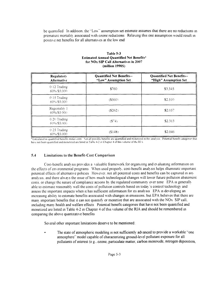
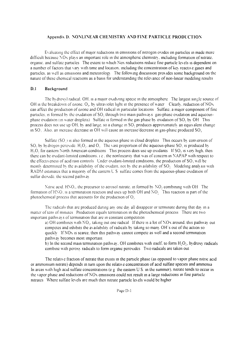
3.4 Nitrogen Deposition Estimates
Nitrogen deposition estimates are generated using RADM The RADM was de\ eloped over a ten
\earperiod. 1984 - 1993. under the auspices of the National Acid Precipitation  Assessment
 Program to
address polic> and technical issues associated \\ith acidic deposition The model is designed to provide a
scientific basis for predicting changes in deposition and air quality resulting from changes in precursor
emissions and to predict the levels of acidic deposition in certain sensitn e receptor regions To do so requires
that RADM be a multipollutant model that predicts the oxidizing capacity of the atmosphere, including the
prediction of o/one. and chemical transformations mvoh ing oxides of sulfur and nitrogen
The de\elopment. application, and e\ aluation of the RADM has been documented extensiveh b>
NAPAP (Chang, et al 1987 & 1990. Dennis et al 1990) RADM has been used in several recent studies of
acidic deposition, including EPA's 1995 Acid Deposition Standard Feasibility Stud) Report to Congress
(U S EPA. 1995). EPA's 1997 Deposition of Air Pollutants to the Great Waters Report to Congress (U S
EPA. 1997e). and in \\ork estmatmg the nitrogen deposition airshed of the Chesapeake Bay watershed
(Dennis. 1997)
RADM estimates deposition in units of kilograms per hectare (kg/ha) Wet deposition is estimated
in the form of SO;:\ NO,". NH3. H" Dr> deposition is estimated in the form of S0:. SO., as aerosol. 0_,.
HNO-,. NO,. H-O^ The deposition estimates are mapped to specific East Coast and Gulf Coast estuaries and
their \\atersheds : Land deposited nitrogen in each \\atershed is multiplied b\ a factor of 10% to obtain the
nitrogen load delnered Ma export (pass-through) to the corresponding estuan
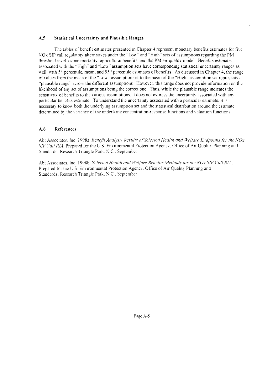
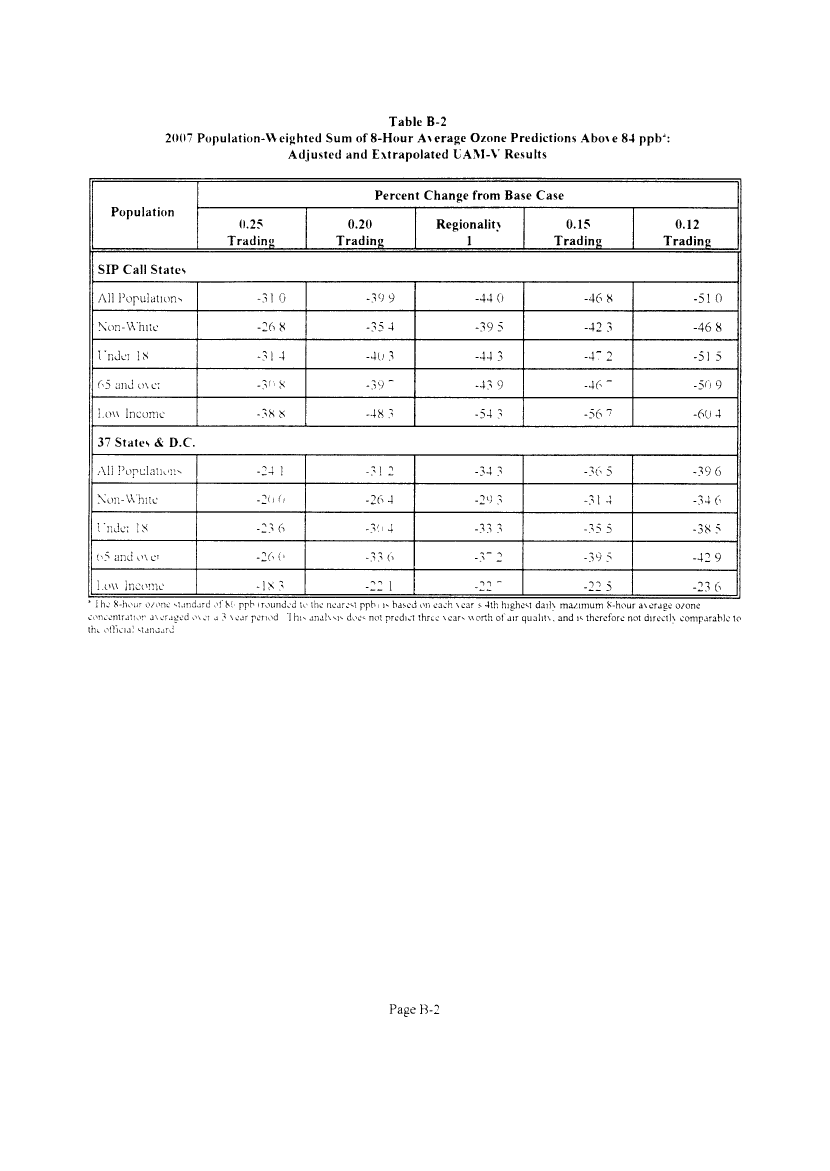
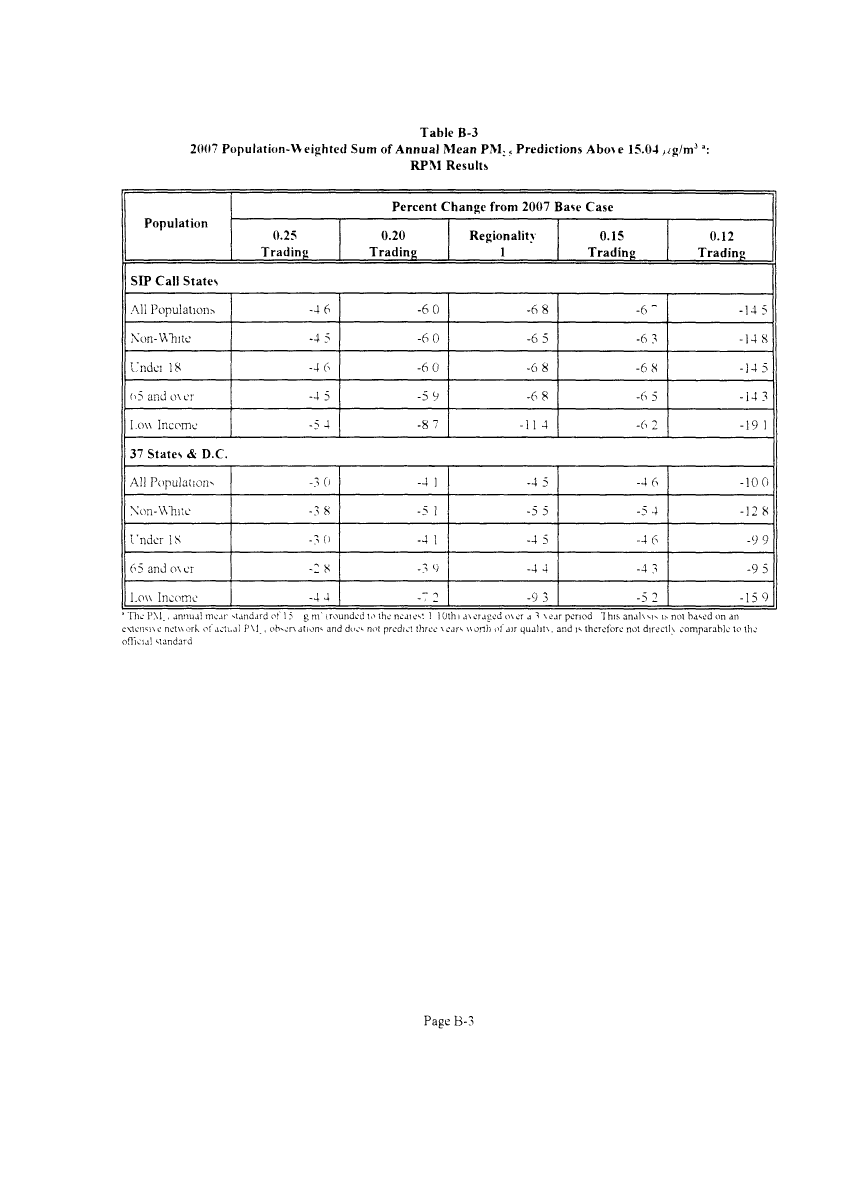
Table 3-4 proxidcs a summan of the nitrogen deposition estimates for each cell in the RADM
domain The changes range from 0 01 kg/ha to 3 66 kg/ha The results for the 0 15 option represent an 11%
reduction in the a\eragc annual deposition across the entire domain The air qualiU technical support
document for this R1A (Abt Associates. 1998) contains maps sho\\mg the nitrogen deposition changes
generated using RADM for each of fi\e regulators altcrnatnes (0 25 Trading. 0 20 Trading. Regionally 1.
0 15 Trading, and 0 12 Trading) Another technical support document for this RJA (EPA. 1998d) contains
additional information on the reduction in mtroaen loads to 12 stud\ set estuaries
'• F.PA has de\eloped a methodology to assess nitrogen deposition benefits direct!) for 12 different estuaries
Albemarle,' Pamhco Sounds. Cape Cod Ba\. Chesapeake Ba\. Delaware Bay, Delaware Inland Ba\s. Gardmers Ba\.
Hudson R •' Rantan Ba\. Long Island Sound. Massachusetts Ba}. Narragansett Ba>. Sarasota Ba\. and Tampa Ba\
Page 3-19
image:
Program to
address polic> and technical issues associated \\ith acidic deposition The model is designed to provide a
scientific basis for predicting changes in deposition and air quality resulting from changes in precursor
emissions and to predict the levels of acidic deposition in certain sensitn e receptor regions To do so requires
that RADM be a multipollutant model that predicts the oxidizing capacity of the atmosphere, including the
prediction of o/one. and chemical transformations mvoh ing oxides of sulfur and nitrogen
The de\elopment. application, and e\ aluation of the RADM has been documented extensiveh b>
NAPAP (Chang, et al 1987 & 1990. Dennis et al 1990) RADM has been used in several recent studies of
acidic deposition, including EPA's 1995 Acid Deposition Standard Feasibility Stud) Report to Congress
(U S EPA. 1995). EPA's 1997 Deposition of Air Pollutants to the Great Waters Report to Congress (U S
EPA. 1997e). and in \\ork estmatmg the nitrogen deposition airshed of the Chesapeake Bay watershed
(Dennis. 1997)
RADM estimates deposition in units of kilograms per hectare (kg/ha) Wet deposition is estimated
in the form of SO;:\ NO,". NH3. H" Dr> deposition is estimated in the form of S0:. SO., as aerosol. 0_,.
HNO-,. NO,. H-O^ The deposition estimates are mapped to specific East Coast and Gulf Coast estuaries and
their \\atersheds : Land deposited nitrogen in each \\atershed is multiplied b\ a factor of 10% to obtain the
nitrogen load delnered Ma export (pass-through) to the corresponding estuan
Table 3-4 proxidcs a summan of the nitrogen deposition estimates for each cell in the RADM
domain The changes range from 0 01 kg/ha to 3 66 kg/ha The results for the 0 15 option represent an 11%
reduction in the a\eragc annual deposition across the entire domain The air qualiU technical support
document for this R1A (Abt Associates. 1998) contains maps sho\\mg the nitrogen deposition changes
generated using RADM for each of fi\e regulators altcrnatnes (0 25 Trading. 0 20 Trading. Regionally 1.
0 15 Trading, and 0 12 Trading) Another technical support document for this RJA (EPA. 1998d) contains
additional information on the reduction in mtroaen loads to 12 stud\ set estuaries
'• F.PA has de\eloped a methodology to assess nitrogen deposition benefits direct!) for 12 different estuaries
Albemarle,' Pamhco Sounds. Cape Cod Ba\. Chesapeake Ba\. Delaware Bay, Delaware Inland Ba\s. Gardmers Ba\.
Hudson R •' Rantan Ba\. Long Island Sound. Massachusetts Ba}. Narragansett Ba>. Sarasota Ba\. and Tampa Ba\
Page 3-19
image:
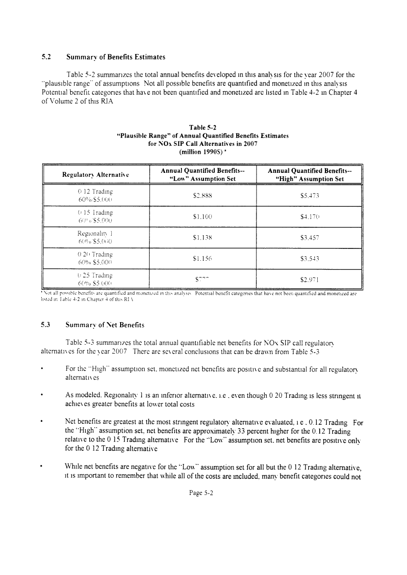
 Table 3-3
Summan of S-R Matrix Derived PM Air Qualin
Statistic
Minimum Annual Mean
PM,( (..g'mV'
Maximum Annual Mean
>Mir, (..g'nV) !
A\cragc .Annual Mean
3M,, (. gm''i
Population-\\ eighted
A\ erage Annual Mean
5M (person-, e'mV
Minimum Annual Mean
PM:,(. g'mV
Maximum Annual Mean
PM-, (..g'mV
A\ erage /Vnnual Mean
PM- . f . g m'i
Population- Weighted
A\ erage Annual Mean
PM- , (person-, e'm' i l
2007 Base
Case
539
66 3"
2262
25 96
3 49
2~ 63
10 "4
1262
Change Relath e To 2007 Base Case "
0.25
Trading
-0 56
020
-0 03
-0 03
-052
0 20
-00?
-0 03
0.20
Trading
-056
021
-003
-004
-052
021
-0 03
-0 04
Reg. 1
-053
026
-002
-0 03
-049
025
-0 02
-0 03
0.15
Trading
-057
026
-004
-004
-053
026
-0 04
-004
0.12
Trading
-0 6"
0 16
-0 06
-o u"
-0 6~
0 17
-0 05
-0 06
The chanec is defined as the eontrol case \alue minus the ba*-e ease \ alue
s The base ^a-.e minimum i maximum) is the \alue tor the counu uith the louest (highest) annual average The change relatne to ih
the minimum i maximum i from the set of ehange-. in all counties
• Calculated m summmc the product of the protected 2r'0~ counts population and the estimated 2007 counts P\I concentration and
the total populalior in the 3 1 sute^ modeled u^mg the S-R Matrix
; base case picks
then dr. idi:iL r.'-
Population-weighted air quahtx changes \\ere not estimated using the S-R Matrix results The
results generated from the RPM modeling sho\vn in Appendix B should be generalh representalne of the
direction and magnitude of changes that would be estimated using the S-R Matrix results
The air qualm technical support document for this R1A (Abt Associates. 1998) contains maps
showing the base case PM concentrations and PM concentration changes generated using the S-R Matrix for
each of fi\ e regulator) alternatives (0 25 Trading. 0.20 Trading. Regionally 1.015 Trading, and 0 12
Trading) Similar maps can also be found in Pechan. 1998
Page 3-18
image:
Table 3-3
Summan of S-R Matrix Derived PM Air Qualin
Statistic
Minimum Annual Mean
PM,( (..g'mV'
Maximum Annual Mean
>Mir, (..g'nV) !
A\cragc .Annual Mean
3M,, (. gm''i
Population-\\ eighted
A\ erage Annual Mean
5M (person-, e'mV
Minimum Annual Mean
PM:,(. g'mV
Maximum Annual Mean
PM-, (..g'mV
A\ erage /Vnnual Mean
PM- . f . g m'i
Population- Weighted
A\ erage Annual Mean
PM- , (person-, e'm' i l
2007 Base
Case
539
66 3"
2262
25 96
3 49
2~ 63
10 "4
1262
Change Relath e To 2007 Base Case "
0.25
Trading
-0 56
020
-0 03
-0 03
-052
0 20
-00?
-0 03
0.20
Trading
-056
021
-003
-004
-052
021
-0 03
-0 04
Reg. 1
-053
026
-002
-0 03
-049
025
-0 02
-0 03
0.15
Trading
-057
026
-004
-004
-053
026
-0 04
-004
0.12
Trading
-0 6"
0 16
-0 06
-o u"
-0 6~
0 17
-0 05
-0 06
The chanec is defined as the eontrol case \alue minus the ba*-e ease \ alue
s The base ^a-.e minimum i maximum) is the \alue tor the counu uith the louest (highest) annual average The change relatne to ih
the minimum i maximum i from the set of ehange-. in all counties
• Calculated m summmc the product of the protected 2r'0~ counts population and the estimated 2007 counts P\I concentration and
the total populalior in the 3 1 sute^ modeled u^mg the S-R Matrix
; base case picks
then dr. idi:iL r.'-
Population-weighted air quahtx changes \\ere not estimated using the S-R Matrix results The
results generated from the RPM modeling sho\vn in Appendix B should be generalh representalne of the
direction and magnitude of changes that would be estimated using the S-R Matrix results
The air qualm technical support document for this R1A (Abt Associates. 1998) contains maps
showing the base case PM concentrations and PM concentration changes generated using the S-R Matrix for
each of fi\ e regulator) alternatives (0 25 Trading. 0.20 Trading. Regionally 1.015 Trading, and 0 12
Trading) Similar maps can also be found in Pechan. 1998
Page 3-18
image:
 1997d) The standardi/.ation for temperature and pressure was eliminated from this concentration data based
upon proposed rc\ isions to the reference method for PM,,, "
Because there is little PM,, monitoring data a\ ailable. a general linear model was de\ eloped to
predict PM,« concentrations directh from the 1993 - 1995 PMKJ \alues (U S EPA. 1996b) A SASrN1
general linear model (i c . GLM) procedure \\as used to predict PM;< values (dependent \anable) as a
function of independent ^ anables for season, region, and measured PMU. value These dern ed PM; 5 data
\\ere used to calibrate model predictions of annual average PM:5
3.3.5 Development of Annual Median PM2 ? Concentrations
The CRDM procedure does not direct!} produce estimates of daih 24-hour a\erage PM
concentrations or annual median PM concentrations Some health benefits have concentration-response
functions that reh on estimates of either the daih 24-hour average or annual median concentrations Using
historical data. EPA de\ eloped 24-hour a\erage estimates corresponding to the 99th percentile A alue for PM
and the 98th percentile \ alue for PM, ^ reflecting forms of PM,,, and PM:, daih standards
Peak-to-mean ratios (i e . ratio of the 24-hour a\erge value to annual a\erage \alue) are established
from actual PM,, monitor data for 1993 to 1995 from Tier 1 through Tier 3 monitored counties For PMK,.
the peak \ alue is defined cxacth the \\a> it is for the new PMK, NAAQS. i e . the \ alue corresponding to the
99th percentile \aluc of the distribution of actual daih 24-hour a\eragc PM,,, \alues For PM:5. the peak
value is also defined exactly the \\ay it is for the ne\\ PM,, NAAQS. i e . the \ alue corresponding to the 98th
percentile \ alue of the distribution of estimated daih 24-hour a\ erage PM:, \ alues These historical peak-to-
mean ratios for each monitored count} are assumed to hold for the 2007 model \ear in this anah sis and arc
applied to the annual a\ erage PM estimates generated b> the S-R Matrix Peak \ alues in nonmomtored
counties are estimated using the regional a^ erage peak-to-mean ratios in Tier 1 monitored counties
Starting with the annual mean and peak values de\ eloped from the S-R Matrix, maximum likelihood
is then used to estimate the parameters of a Gamma distribution that are most consistent \\ith the S-R Matrix
results The parameters of the Gamma distribution are then used to estimate the annual median concentration
and the concentration corresponding to each decile of the distribution
3.3.6 S-R Matrix PM Air Quality Results
Table 3-3 pro\ ides a summan of the predicted ambient PM,, and PM: s concentrations used in this
stud\ Similar to the results using the RPM approach, the concentration changes are general!} ven small
For the 0 15 option, annual mean PM,,, changes range from an increase of 0 26 ug/m3 to a decrease of-0 57
tig/m3. with an average annual mean change across the 31 state domain of -0 04 ^g/m? Therefore, the
absolute changes in PM occur within a slightly wider band than with the RPM. and the average annual mean
change is slightly lo\\er (-0 04 ,^.g/m3 \ersus -0 06 ^,g/m3)
" See Appendix .1 - Reference Method for PM10, Final Rule for National Ambient Air Quahn Standards for
Paniculate Matter (Federal Register. Vol 62. No 138. p 41. July 18. 1997)
Page 3-17
image:
1997d) The standardi/.ation for temperature and pressure was eliminated from this concentration data based
upon proposed rc\ isions to the reference method for PM,,, "
Because there is little PM,, monitoring data a\ ailable. a general linear model was de\ eloped to
predict PM,« concentrations directh from the 1993 - 1995 PMKJ \alues (U S EPA. 1996b) A SASrN1
general linear model (i c . GLM) procedure \\as used to predict PM;< values (dependent \anable) as a
function of independent ^ anables for season, region, and measured PMU. value These dern ed PM; 5 data
\\ere used to calibrate model predictions of annual average PM:5
3.3.5 Development of Annual Median PM2 ? Concentrations
The CRDM procedure does not direct!} produce estimates of daih 24-hour a\erage PM
concentrations or annual median PM concentrations Some health benefits have concentration-response
functions that reh on estimates of either the daih 24-hour average or annual median concentrations Using
historical data. EPA de\ eloped 24-hour a\erage estimates corresponding to the 99th percentile A alue for PM
and the 98th percentile \ alue for PM, ^ reflecting forms of PM,,, and PM:, daih standards
Peak-to-mean ratios (i e . ratio of the 24-hour a\erge value to annual a\erage \alue) are established
from actual PM,, monitor data for 1993 to 1995 from Tier 1 through Tier 3 monitored counties For PMK,.
the peak \ alue is defined cxacth the \\a> it is for the new PMK, NAAQS. i e . the \ alue corresponding to the
99th percentile \aluc of the distribution of actual daih 24-hour a\eragc PM,,, \alues For PM:5. the peak
value is also defined exactly the \\ay it is for the ne\\ PM,, NAAQS. i e . the \ alue corresponding to the 98th
percentile \ alue of the distribution of estimated daih 24-hour a\ erage PM:, \ alues These historical peak-to-
mean ratios for each monitored count} are assumed to hold for the 2007 model \ear in this anah sis and arc
applied to the annual a\ erage PM estimates generated b> the S-R Matrix Peak \ alues in nonmomtored
counties are estimated using the regional a^ erage peak-to-mean ratios in Tier 1 monitored counties
Starting with the annual mean and peak values de\ eloped from the S-R Matrix, maximum likelihood
is then used to estimate the parameters of a Gamma distribution that are most consistent \\ith the S-R Matrix
results The parameters of the Gamma distribution are then used to estimate the annual median concentration
and the concentration corresponding to each decile of the distribution
3.3.6 S-R Matrix PM Air Quality Results
Table 3-3 pro\ ides a summan of the predicted ambient PM,, and PM: s concentrations used in this
stud\ Similar to the results using the RPM approach, the concentration changes are general!} ven small
For the 0 15 option, annual mean PM,,, changes range from an increase of 0 26 ug/m3 to a decrease of-0 57
tig/m3. with an average annual mean change across the 31 state domain of -0 04 ^g/m? Therefore, the
absolute changes in PM occur within a slightly wider band than with the RPM. and the average annual mean
change is slightly lo\\er (-0 04 ,^.g/m3 \ersus -0 06 ^,g/m3)
" See Appendix .1 - Reference Method for PM10, Final Rule for National Ambient Air Quahn Standards for
Paniculate Matter (Federal Register. Vol 62. No 138. p 41. July 18. 1997)
Page 3-17
image:
 To address this bias, a multiplicatne factor of 0 25 is applied national!) to fugitn e dust emissions as
a reasonable first-order attempt to reconcile differences between modeled predictions of PiYL ^ and actual
ambient data This is the same adjustment that \\as used in the 1997 PM NAAQS RIA A 0 25
multiphcatn e adjustment results in a fugitn e dust contribution to modeled ambient PM;, concentrations of
10% to 17% " E\en after this adjustment the fugitne dust fraction of total eastern PM:^ mass is 104%.
which is still greater than the 5% indicated by IMPROVE monitors Ho\ve-\ er: given that the 0 25
multiphcatn e factor appears to bring the modeled fugitn e dust contribution to PM: 5 mass more within the
range of \ alues reported from speciated monitoring data, the fugitive dust contribution to total PM that is
estimated b> the S-R Matrix is adjusted by this factor Since this factor still max result in an overprediction
of the fugitne dust contribution, the S-R Matrix may tend to underpredict the effectneness of strategics that
affect NSA
3.3.4 Normalizing S-R Matrix Results to Measured Data
In an attempt to further ensure comparability between S-R Matrix results and measured annual
a\ eragc PM \ alues. the S-R results are calibrated using factors de\ eloped for the PM and Ozone NAAQS
RIA (U S EPA. 1997a) For the NAAQS RIA. a "normalization factor" \\as de\ eloped for each Tier 1 to
Tier 3 monitored count} :' Nonmomtored counties \\ere calibrated using the appropriate regional
normah/ation factor calculated as the a\erage of Tier 1 normalization factors across a en'en modeling region
The normah/ation factor was calculated as the monitored \ alue dn ided b> the modeled value
All S-R Matrix predictions \\ere normalized regardless of overprediction or underprediction relatne
to monitored \ alues This factor \\as applied equalh across all particle species contributing to the annual
a\erage PM \aluc at a count)-le\ el receptor
The calibration procedure \\as conducted emplo\mg 1993 - 1995 PMlu ambient monitoring data
from the AIRS database following the air quaht) tier data completeness parameters discussed abo\c The
PM; data represent the annual a\erage of design value monitors a\eraged o\er three years (U S EPA.
"" Sec l: S EPA 199 'b. page 6-5 for a map delineating modeling region Using 0 25 mulliphcame factoi.
fugime dust as percentage of P.M. = mass for Central US =1" 2%. Eastern U S = 104%. Western U S = 10 6% B>
comparison, \\ithout using a multiphcame factor, fugitn c dust as a percentage of PM., mass for Central US =44 6%
Eastern U S = .10 9%. Western U S =31 5%
10 The normalization procedure was conducted for count) -\e\ el modeled PM10 and PM;, estimates falling into
one of four air qualit) data tiers The tiering scheme reflects increasing relaxation of data completeness criteria and
therefore increasing uncertainty for the annual design \alue (U S EPA. 1997f) Nationwide. Tier 1 monitored counties
co\er the 504 counties \\ith at least 50% data completeness and therefore have the highest level of certainty associated
with the annual design value Tier 2 monitored counties cover 100 additional counties \Mth at least one data point (i e .
one 24-hour value) for each of the three \ears during the period 1993 -1995 Tier 3 monitored counties cover 107
additional counties u ith missing monitoring data for one or tw o of the three) ears 1993-1995 In total. Tiers 1. 2 and 3
co\er7H counties currenth monitored for PM10 in the 48 contiguous states In 1997 the PM,0 monitoring network
consisted of approximate!;* 1600 individual monitors with a coverage of approximate!) 711 counties in the 48
contiguous states Tier 4 covers the remaining 2369 nonmomtored counties
Page 3-16
image:
To address this bias, a multiplicatne factor of 0 25 is applied national!) to fugitn e dust emissions as
a reasonable first-order attempt to reconcile differences between modeled predictions of PiYL ^ and actual
ambient data This is the same adjustment that \\as used in the 1997 PM NAAQS RIA A 0 25
multiphcatn e adjustment results in a fugitn e dust contribution to modeled ambient PM;, concentrations of
10% to 17% " E\en after this adjustment the fugitne dust fraction of total eastern PM:^ mass is 104%.
which is still greater than the 5% indicated by IMPROVE monitors Ho\ve-\ er: given that the 0 25
multiphcatn e factor appears to bring the modeled fugitn e dust contribution to PM: 5 mass more within the
range of \ alues reported from speciated monitoring data, the fugitive dust contribution to total PM that is
estimated b> the S-R Matrix is adjusted by this factor Since this factor still max result in an overprediction
of the fugitne dust contribution, the S-R Matrix may tend to underpredict the effectneness of strategics that
affect NSA
3.3.4 Normalizing S-R Matrix Results to Measured Data
In an attempt to further ensure comparability between S-R Matrix results and measured annual
a\ eragc PM \ alues. the S-R results are calibrated using factors de\ eloped for the PM and Ozone NAAQS
RIA (U S EPA. 1997a) For the NAAQS RIA. a "normalization factor" \\as de\ eloped for each Tier 1 to
Tier 3 monitored count} :' Nonmomtored counties \\ere calibrated using the appropriate regional
normah/ation factor calculated as the a\erage of Tier 1 normalization factors across a en'en modeling region
The normah/ation factor was calculated as the monitored \ alue dn ided b> the modeled value
All S-R Matrix predictions \\ere normalized regardless of overprediction or underprediction relatne
to monitored \ alues This factor \\as applied equalh across all particle species contributing to the annual
a\erage PM \aluc at a count)-le\ el receptor
The calibration procedure \\as conducted emplo\mg 1993 - 1995 PMlu ambient monitoring data
from the AIRS database following the air quaht) tier data completeness parameters discussed abo\c The
PM; data represent the annual a\erage of design value monitors a\eraged o\er three years (U S EPA.
"" Sec l: S EPA 199 'b. page 6-5 for a map delineating modeling region Using 0 25 mulliphcame factoi.
fugime dust as percentage of P.M. = mass for Central US =1" 2%. Eastern U S = 104%. Western U S = 10 6% B>
comparison, \\ithout using a multiphcame factor, fugitn c dust as a percentage of PM., mass for Central US =44 6%
Eastern U S = .10 9%. Western U S =31 5%
10 The normalization procedure was conducted for count) -\e\ el modeled PM10 and PM;, estimates falling into
one of four air qualit) data tiers The tiering scheme reflects increasing relaxation of data completeness criteria and
therefore increasing uncertainty for the annual design \alue (U S EPA. 1997f) Nationwide. Tier 1 monitored counties
co\er the 504 counties \\ith at least 50% data completeness and therefore have the highest level of certainty associated
with the annual design value Tier 2 monitored counties cover 100 additional counties \Mth at least one data point (i e .
one 24-hour value) for each of the three \ears during the period 1993 -1995 Tier 3 monitored counties cover 107
additional counties u ith missing monitoring data for one or tw o of the three) ears 1993-1995 In total. Tiers 1. 2 and 3
co\er7H counties currenth monitored for PM10 in the 48 contiguous states In 1997 the PM,0 monitoring network
consisted of approximate!;* 1600 individual monitors with a coverage of approximate!) 711 counties in the 48
contiguous states Tier 4 covers the remaining 2369 nonmomtored counties
Page 3-16
image:
 • Because ammonium nitrate forms onh under relatively lo\\ temperatures, annual axerage particle
nitrate concentrations are di\ ided b> four assuming that sufficient!) lo\\ temperatures are present
onK one-quarter of the > ear
Final!}. the total particle mass of ammonium sulfate and ammonium nitrate is calculated
For application to the NO\ SIP call, emissions data for onh those counties located in the 37 OTAG
states plus the District of Columbia are used Because nationwide emissions are not used, the S-R Matrix
results are incomplete for air qualih predictions m the counties located in states along the western border of
the OTAG domain For example, emissions from New Mexico are expected to have a significant downwind
impact on ambient PM concentrations in neighboring counties m Texas However. New Mexico emissions
are not estimated in this anal} sis Incomplete air qualit} predictions for the six western border states make
unreliable am anal} sis that imposes a threshold for health effects (see Chapter 11) As shown in Figure 3-3.
EPA has chosen not to include the air quality results from the six "buffer"' states in the benefits anah scs that
are performed using the S-R Matrix results Since the 31 remaining states are generally located more than
525 km (approximate!) 330 miles) from the states for which emissions information is not a\ ailable. the air
qualit} results for the 31 states is belie\ed to be more reliable
3.3.3 Fugitive Dust Adjustment Factor
As indicated in subsection 34 1. the 1990 CRDM predictions for fugitive dust are not consistent
\\ith measured ambient data The CRDM-predicted a\ eragc fugitn e dust contribution to total PM;, mass is
3 1% in the East and 32°«in the West (E H Pechan. 1997b) Speciated monitoring data from the IMPROVE
net\\ork show that minerals (i e . crustal material) comprise approximate!} 5% of PM;< mass in the East and
approximate!) 15°o of PM- < mass in the West (U S EPA. 1996a) These disparate results suggest a
s> stematic o\ erbias in the fugitn c dust contribution to total PM This o\ erestimatc is further complicated b>
the recognition that the 1990 NPI significant!} o\ erestimates fugitn e dust emissions The most recent
National Emissions Trends imcnton indicates that the NPI o\ erestimates fugitn e dust PM,, and PM:,
emissions b} 40% and 73% respectneh" (U S EPA. 1997c)
To calculate total particle mass of ammonium sulfate and ammonium nitrate, the anion concentrations of
sulfate and nitrate are multiplied b\ 1 375 and 1 290 respectneh
8 Natural and man-made fugitive dust emissions account for 86% of PM10 emissions and 59% of P.M.,
emissions in the most recent 1990 estimates in the National Emission Trends Inventon
Page 3-14
image:
• Because ammonium nitrate forms onh under relatively lo\\ temperatures, annual axerage particle
nitrate concentrations are di\ ided b> four assuming that sufficient!) lo\\ temperatures are present
onK one-quarter of the > ear
Final!}. the total particle mass of ammonium sulfate and ammonium nitrate is calculated
For application to the NO\ SIP call, emissions data for onh those counties located in the 37 OTAG
states plus the District of Columbia are used Because nationwide emissions are not used, the S-R Matrix
results are incomplete for air qualih predictions m the counties located in states along the western border of
the OTAG domain For example, emissions from New Mexico are expected to have a significant downwind
impact on ambient PM concentrations in neighboring counties m Texas However. New Mexico emissions
are not estimated in this anal} sis Incomplete air qualit} predictions for the six western border states make
unreliable am anal} sis that imposes a threshold for health effects (see Chapter 11) As shown in Figure 3-3.
EPA has chosen not to include the air quality results from the six "buffer"' states in the benefits anah scs that
are performed using the S-R Matrix results Since the 31 remaining states are generally located more than
525 km (approximate!) 330 miles) from the states for which emissions information is not a\ ailable. the air
qualit} results for the 31 states is belie\ed to be more reliable
3.3.3 Fugitive Dust Adjustment Factor
As indicated in subsection 34 1. the 1990 CRDM predictions for fugitive dust are not consistent
\\ith measured ambient data The CRDM-predicted a\ eragc fugitn e dust contribution to total PM;, mass is
3 1% in the East and 32°«in the West (E H Pechan. 1997b) Speciated monitoring data from the IMPROVE
net\\ork show that minerals (i e . crustal material) comprise approximate!} 5% of PM;< mass in the East and
approximate!) 15°o of PM- < mass in the West (U S EPA. 1996a) These disparate results suggest a
s> stematic o\ erbias in the fugitn c dust contribution to total PM This o\ erestimatc is further complicated b>
the recognition that the 1990 NPI significant!} o\ erestimates fugitn e dust emissions The most recent
National Emissions Trends imcnton indicates that the NPI o\ erestimates fugitn e dust PM,, and PM:,
emissions b} 40% and 73% respectneh" (U S EPA. 1997c)
To calculate total particle mass of ammonium sulfate and ammonium nitrate, the anion concentrations of
sulfate and nitrate are multiplied b\ 1 375 and 1 290 respectneh
8 Natural and man-made fugitive dust emissions account for 86% of PM10 emissions and 59% of P.M.,
emissions in the most recent 1990 estimates in the National Emission Trends Inventon
Page 3-14
image:
 because it relates closeh to 1990 emissions and meteorological data used in the CRDM Since the
IMPROVE network monitors are primanh concerned with e\aluatmg visibility impairment in predominant!}
rural Class I areas, these comparisons are incomplete due to the lack of coverage in urban areas With the
exception of the fugitne dust component of PM: * and PM1(1. modeled and measured concentrations of sulfate.
nitrate and organics are comparable (Latimer. 1996)
The CRDM has also been benchmarked against the RADM-RPM for the Eastern U S using 1990
emissions and meteorology (U S EPA. 1997b) RADM-RPM incorporates more comprehensn e physics and
chemistry to enable better characterization of secondarih -formed pollutants than Lagrangian-based methods
In general, the CRDM results shew a similar trend in sulfate and nitrate concentrations \\ithm the same
modeling region Also, the CRDM-predicted annual a\ erage concentrations of sulfate are within the range of
RADM-RPM base-case predictions Relative to RADM-RPM base case results. CRDM appears to
o\erpredict nitrate concentrations in the Midwest and underpredict nitrate concentrations in the Mid-Atlantic
states
3.3.2 Development of the S-R Matrix
To de^elop the S-R Matrix, a nationwide total of 5.944 sources (i e . industrial point, utility area.
nonroad. and motor \ chicle) of pnmaiy and precursor emissions were modeled with CRDM In addition.
secondary organic aerosols formed from anthropogenic and biogemc VOC emissions were modeled Natural
sources of PM, and PM:, (i e . \\ind erosion and wild fires) \\ere also included Emissions of SO:. NOx. and
ammonia were modeled in order to calculate ammonium sulfate and ammonium nitrate concentrations, the
pnmarx particulate forms of sulfate and nitrate The CRDM produced a matrix of transfer coefficients for
each of these primary and particulate precursor pollutants These coefficients can be applied to the emissions
of am unit (area source or indnidual point source) to calculate a particular source's contribution to a county
receptor's total annual a\ erage PM,,, or PM; < concentration Each indrudual unit in the imentory is
associated \\ith one of the modeled source types (i e . area, point sources with effectne stack height of 0 to
250 m. 250 m to 500 m. and mdnidual point sources \sith effectne stack height abo\e 500 m) for each
county
The S-R Matrix transfer coefficients \\ere adjusted to reflect concentrations of secondanh-formed
participates (Latimer. 1996) First, the transfer coefficients for SO;. NOx. and ammonia \\ere multiplied b>
the ratios of the molecular \\eights of sulfate/SO-. nitrate/nitrogen dioxide and ammonium/ammonia to obtain
concentrations of sulfate. nitrate and ammonium 6 The relatne concentrations in the atmosphere of
ammonium sulfate and ammonium nitrate depend on complex chemical reactions In the presence of sulfate
and nitric acid (the gas phase oxidation product of NOx). ammonia reacts preferential!} \\ith sulfate to form
particulate ammonium sulfate rather than react with nitric acid to form particulate ammonium nitrate Under
conditions of excess ammonium and low temperatures, ammonium nitrate forms For each county receptor.
the sulfate-nitrate-ammonmm equilibrium is estimated based on the following simphfing assumptions
• All sulfate is neutralized b\ ammonium.
• Ammonium nitrate forms onh when there is excess ammonium.
1 Ratio of molecular \\eights Sulfate/SCK= 1 50. nitrate/nitrogen dioxide = 1 35. ammonium/ammonia = 1 06
Page 3-13
image:
because it relates closeh to 1990 emissions and meteorological data used in the CRDM Since the
IMPROVE network monitors are primanh concerned with e\aluatmg visibility impairment in predominant!}
rural Class I areas, these comparisons are incomplete due to the lack of coverage in urban areas With the
exception of the fugitne dust component of PM: * and PM1(1. modeled and measured concentrations of sulfate.
nitrate and organics are comparable (Latimer. 1996)
The CRDM has also been benchmarked against the RADM-RPM for the Eastern U S using 1990
emissions and meteorology (U S EPA. 1997b) RADM-RPM incorporates more comprehensn e physics and
chemistry to enable better characterization of secondarih -formed pollutants than Lagrangian-based methods
In general, the CRDM results shew a similar trend in sulfate and nitrate concentrations \\ithm the same
modeling region Also, the CRDM-predicted annual a\ erage concentrations of sulfate are within the range of
RADM-RPM base-case predictions Relative to RADM-RPM base case results. CRDM appears to
o\erpredict nitrate concentrations in the Midwest and underpredict nitrate concentrations in the Mid-Atlantic
states
3.3.2 Development of the S-R Matrix
To de^elop the S-R Matrix, a nationwide total of 5.944 sources (i e . industrial point, utility area.
nonroad. and motor \ chicle) of pnmaiy and precursor emissions were modeled with CRDM In addition.
secondary organic aerosols formed from anthropogenic and biogemc VOC emissions were modeled Natural
sources of PM, and PM:, (i e . \\ind erosion and wild fires) \\ere also included Emissions of SO:. NOx. and
ammonia were modeled in order to calculate ammonium sulfate and ammonium nitrate concentrations, the
pnmarx particulate forms of sulfate and nitrate The CRDM produced a matrix of transfer coefficients for
each of these primary and particulate precursor pollutants These coefficients can be applied to the emissions
of am unit (area source or indnidual point source) to calculate a particular source's contribution to a county
receptor's total annual a\ erage PM,,, or PM; < concentration Each indrudual unit in the imentory is
associated \\ith one of the modeled source types (i e . area, point sources with effectne stack height of 0 to
250 m. 250 m to 500 m. and mdnidual point sources \sith effectne stack height abo\e 500 m) for each
county
The S-R Matrix transfer coefficients \\ere adjusted to reflect concentrations of secondanh-formed
participates (Latimer. 1996) First, the transfer coefficients for SO;. NOx. and ammonia \\ere multiplied b>
the ratios of the molecular \\eights of sulfate/SO-. nitrate/nitrogen dioxide and ammonium/ammonia to obtain
concentrations of sulfate. nitrate and ammonium 6 The relatne concentrations in the atmosphere of
ammonium sulfate and ammonium nitrate depend on complex chemical reactions In the presence of sulfate
and nitric acid (the gas phase oxidation product of NOx). ammonia reacts preferential!} \\ith sulfate to form
particulate ammonium sulfate rather than react with nitric acid to form particulate ammonium nitrate Under
conditions of excess ammonium and low temperatures, ammonium nitrate forms For each county receptor.
the sulfate-nitrate-ammonmm equilibrium is estimated based on the following simphfing assumptions
• All sulfate is neutralized b\ ammonium.
• Ammonium nitrate forms onh when there is excess ammonium.
1 Ratio of molecular \\eights Sulfate/SCK= 1 50. nitrate/nitrogen dioxide = 1 35. ammonium/ammonia = 1 06
Page 3-13
image:
 Table 3-2
Summar} of RPM Derived PM Air Quality
Statistic
Minimum Annual Moan
PMlcu;g'nV)b
Maximum Annual Mean
PM;0 (-g'mV
A\erage Annual Mean
PM : (,. g rn'i
Population-Weighted
A\erage Annual Mean
PM ^ (person-, g'm'i '
Minimum Annual Mean
PM:. (.-g rrf) "
Maximum .Annual Mean
PM:,L.g''mV
A\ erage Annual Mean
PM:< (. g;m"')
Population -\\'eighted
A\ erase Annual Mean
PM,, (person-, g m'> '
2007 Base
Case
1545
3591
26 76
26 46
665
22 63
1 4 96
14 53
Change Relathe to 2007 Base Case2
0.25
Trading
-049
024
-( i 04
-0 03
-(|49
024
.0 04
-003
0.20
Trading
-046
024
-005
-0 05
-0 46
024
-0 05
-0 05
Reg. 1
-045
026
-005
-005
-0 45
026
-0 05
-0 05
0.15
Trading
-049
029
-006
-0 05
-049
029
-006
-005
0.12
Trading
-052
0 18
-0 12
-0 13
-052
0 18
-0 12
-0 1 3
1 The change i1- defined as the Control ca--e \a!ue minus the base case %a!ue Note that there is no difference between the changes in PM;« and ]
because R U)M RPM onl\ estimates the change in nitrates and sullates \\hich are both in the PM_. fraction
1 1 he hase case minimum (ma\mium > is the \ aluc for the «.ounu \\ ith the lo\\est (highest) annual a\ erage The change relati\e to the base case picks
the minimum (maximum i irom the ->et oi changes m all countie*-
' C alculaled b% summing the product oflhc pro] jclcd 2r>()~ counl\ population and the estimated 2007 counl> PM concentration, and then di\ idinc b\
the total population
3.3.1 Climatological Regional Dispersion Model
The CRDM uses assumptions similar to the Industrial Source Complex Short Term (ISCST?). an
EPA-recommended short range Gaussian dispersion model CRDM incorporates terms for wet and dn
deposition and chemical comersion of S0: and N0\. and uses climatological summaries (annual average
mixing heights and joint frequency distributions of wind speed and direction) from 100 upper air
meteorological sites throughout North America Meterological data for 1990 coupled with emissions data
from version 2 0 of the 1990 National Paniculate Imenton were used to develop the S-R Matrix
In order to evaluate the performance of the Phase II CRDM. model-predicted PM concentrations and
measured ambient PM concentrations were compared Measured annual average PM concentrations b\
chemical species from the Interagency Monitoring for Protection of Visual Enuronments (IMPROVE)
network \\ere examined for the three-year period March 1988 - February 1991 This period was chosen
Page 3-12
image:
Table 3-2
Summar} of RPM Derived PM Air Quality
Statistic
Minimum Annual Moan
PMlcu;g'nV)b
Maximum Annual Mean
PM;0 (-g'mV
A\erage Annual Mean
PM : (,. g rn'i
Population-Weighted
A\erage Annual Mean
PM ^ (person-, g'm'i '
Minimum Annual Mean
PM:. (.-g rrf) "
Maximum .Annual Mean
PM:,L.g''mV
A\ erage Annual Mean
PM:< (. g;m"')
Population -\\'eighted
A\ erase Annual Mean
PM,, (person-, g m'> '
2007 Base
Case
1545
3591
26 76
26 46
665
22 63
1 4 96
14 53
Change Relathe to 2007 Base Case2
0.25
Trading
-049
024
-( i 04
-0 03
-(|49
024
.0 04
-003
0.20
Trading
-046
024
-005
-0 05
-0 46
024
-0 05
-0 05
Reg. 1
-045
026
-005
-005
-0 45
026
-0 05
-0 05
0.15
Trading
-049
029
-006
-0 05
-049
029
-006
-005
0.12
Trading
-052
0 18
-0 12
-0 13
-052
0 18
-0 12
-0 1 3
1 The change i1- defined as the Control ca--e \a!ue minus the base case %a!ue Note that there is no difference between the changes in PM;« and ]
because R U)M RPM onl\ estimates the change in nitrates and sullates \\hich are both in the PM_. fraction
1 1 he hase case minimum (ma\mium > is the \ aluc for the «.ounu \\ ith the lo\\est (highest) annual a\ erage The change relati\e to the base case picks
the minimum (maximum i irom the ->et oi changes m all countie*-
' C alculaled b% summing the product oflhc pro] jclcd 2r>()~ counl\ population and the estimated 2007 counl> PM concentration, and then di\ idinc b\
the total population
3.3.1 Climatological Regional Dispersion Model
The CRDM uses assumptions similar to the Industrial Source Complex Short Term (ISCST?). an
EPA-recommended short range Gaussian dispersion model CRDM incorporates terms for wet and dn
deposition and chemical comersion of S0: and N0\. and uses climatological summaries (annual average
mixing heights and joint frequency distributions of wind speed and direction) from 100 upper air
meteorological sites throughout North America Meterological data for 1990 coupled with emissions data
from version 2 0 of the 1990 National Paniculate Imenton were used to develop the S-R Matrix
In order to evaluate the performance of the Phase II CRDM. model-predicted PM concentrations and
measured ambient PM concentrations were compared Measured annual average PM concentrations b\
chemical species from the Interagency Monitoring for Protection of Visual Enuronments (IMPROVE)
network \\ere examined for the three-year period March 1988 - February 1991 This period was chosen
Page 3-12
image:
 scenario A similar procedure is used to estimate PM x alues in the control scenarios Additional detail on
these procedures can be found in Abt. 1998
3.2.5 RPM PM Air Quality Results
Table 3-2 proMdes a summan of the predicted ambient PM]fj and PM;^ concentrations used in this
stud> Since onl\ the NSA fraction of total PM changes, the estimates of changes for PMir and PM; ^ are
identical The concentration changes are general!} xer\ small For the 0 15 option, annual mean PM changes
range from an increase of 0 29 ug/m3 to a decrease of-0 49 ^g/m\ with an axerage annual mean change
across the RPM domain of -0 06 .'.g/rrf
Population-weighted changes in RPM predicted annual mean PM- 5 and PM,,, concentrations above
the lex el of each ambient air quahu standard are presented in Appendix B These changes are estimated for
the total exposed population and for various subpopulations. including minority groups, children, the elderlx.
and the impox enshed In the SIP call states, the predicted decline in total population exposure abox e the
PM; ^ annual standard le\ el ranges from 5% to 15% There is no predicted change in total population
exposure abo\ e the PM: annual standard lex el because there is no predicted baseline exposure abox e the
standard
The air qualm technical support document for this RIA (Abt Associates. 1998) contains maps
show ing the base case PM concentrations and PM concentration changes generated using RPM for each of
fixe regulator* alternatixes (0 25 Trading. 0 20 Trading. Regionaht} 1.0 15 Trading, and 0 12 Trading)
3.3 PM Air Qualitx Estimates Using the S-R Matrix
The Source-Receptor Matrix (S-R Matrix) reflects the relationship betx\een annual axerage PM
concentration \ alues at a single receptor in each count} (a hypothetical design value monitor sited at the
countx population ccntroid) and the contribution bx PM species to this concentration from each emission
source (E H Pcchan. 1996) The receptors that are modeled include all U S count} centroids plus receptors
in 10 Canadian pro\ mces and 29 Mexican cities/states The methodolog} used in this RIA for estimating PM
air quaht} concentrations using the S-R Matrix is similar to the method used in the Julx 1997 PM and 0/one
NAAQS RIA (U S EPA. 1997a) The S-R Matrix was dexeloped using the Chmatalogical Regional
Dispersion Model (CRDM). and has been calibrated using 1993 - 1995 PM,, and PM:5 monitoring data
These calibration factors, referred to as "normali/ation factors." are applied to all S-R Matrix predictions
Page 3-1
image:
scenario A similar procedure is used to estimate PM x alues in the control scenarios Additional detail on
these procedures can be found in Abt. 1998
3.2.5 RPM PM Air Quality Results
Table 3-2 proMdes a summan of the predicted ambient PM]fj and PM;^ concentrations used in this
stud> Since onl\ the NSA fraction of total PM changes, the estimates of changes for PMir and PM; ^ are
identical The concentration changes are general!} xer\ small For the 0 15 option, annual mean PM changes
range from an increase of 0 29 ug/m3 to a decrease of-0 49 ^g/m\ with an axerage annual mean change
across the RPM domain of -0 06 .'.g/rrf
Population-weighted changes in RPM predicted annual mean PM- 5 and PM,,, concentrations above
the lex el of each ambient air quahu standard are presented in Appendix B These changes are estimated for
the total exposed population and for various subpopulations. including minority groups, children, the elderlx.
and the impox enshed In the SIP call states, the predicted decline in total population exposure abox e the
PM; ^ annual standard le\ el ranges from 5% to 15% There is no predicted change in total population
exposure abo\ e the PM: annual standard lex el because there is no predicted baseline exposure abox e the
standard
The air qualm technical support document for this RIA (Abt Associates. 1998) contains maps
show ing the base case PM concentrations and PM concentration changes generated using RPM for each of
fixe regulator* alternatixes (0 25 Trading. 0 20 Trading. Regionaht} 1.0 15 Trading, and 0 12 Trading)
3.3 PM Air Qualitx Estimates Using the S-R Matrix
The Source-Receptor Matrix (S-R Matrix) reflects the relationship betx\een annual axerage PM
concentration \ alues at a single receptor in each count} (a hypothetical design value monitor sited at the
countx population ccntroid) and the contribution bx PM species to this concentration from each emission
source (E H Pcchan. 1996) The receptors that are modeled include all U S count} centroids plus receptors
in 10 Canadian pro\ mces and 29 Mexican cities/states The methodolog} used in this RIA for estimating PM
air quaht} concentrations using the S-R Matrix is similar to the method used in the Julx 1997 PM and 0/one
NAAQS RIA (U S EPA. 1997a) The S-R Matrix was dexeloped using the Chmatalogical Regional
Dispersion Model (CRDM). and has been calibrated using 1993 - 1995 PM,, and PM:5 monitoring data
These calibration factors, referred to as "normali/ation factors." are applied to all S-R Matrix predictions
Page 3-1
image:
 RPM results, it is neccssan to first use the NSA concentrations to estimate total PM concentrations at each
location under the baseline and each control scenario for the N0\ SIP call'
A first step in using information supplied b> RPM is to estimate distributional statistics for total PM.
using ambient air quaht\ data currenth being developed for the CAAA §812 analysis The location-specific
inputs axailablc from RPM and the upcoming §812 analysis are as follows
« mean and peak PM in the §812 data (PMmean 8!:. PM,,9f, 8]:).
• mean and peak NSA in the §812 data (NSAmcar, 8!:. NSA,,9,, 8::).
• mean, median, and peak NSA in the N0\ SIP call baseline (NSAmean ba,e,Lr,e. NSAm,d ^ basc:i!,e. NSAr .„
i^,,).
• mean, median, and peak NSA in each control scenario of the N'Ox SIP call (NSAmea, ,.,„...,]. NSAniei. ..
„„..,.. NSA, , cor..R.)
Subtracting the mean NSA from mean total PM. one obtains the "other" component of PM (which
includes such components as soil and elemental carbon)
It is assumed that the mean of this (location-specific) "other" component is the same in the NO\ SIP
call baseline as it is in the §812 data
Othern,ea. b<^ ,,c = Othernea. , -
Total PM is estimated in the baseline as
To obtain an estimate of the 90th percentile le\el of PM in the baseline, it is assumed that the
proportion (p) of NSA,ea. ba<eiirt, to PM^ea. t,,,e;^, e is constant across da\s at the same location
P = NSA,,ica: Dfv,_,t / PM,,ed: „,_ = NSA, _ ^ / PM; b_ .
where ; denotes the ;th da\ Gi\en a constant ratio./?, the peak (90th percentile) da\ for baseline PM is the
same da\ as the peak da\ for baseline NSA This implies
In the last step, gnen the mean and 90th percentile point of the distribution of daih PM
concentrations (PMmcd;, babe;me and PM09,, baselme). and assuming that the distribution can be fit well by a
Gamma distribution, the anah sis uses a maximum likelihood estimation to estimate the parameters of the
Gamma distribution that are most consistent with the estimated mean and peak values A distribution of
daih PM values based on NSA components predicted by RPM may then be generated for the baseline
5 The RPM estimates of NSA are anh\ drous estimates However, ambient measurements of NSA do contain
\\ater. which can increase the total NSA mass tn as much as 10% to 50% Therefore, the estimates of total NSA mass
changes derived from RPM understate total NSA mass changes
Page 3-10
image:
RPM results, it is neccssan to first use the NSA concentrations to estimate total PM concentrations at each
location under the baseline and each control scenario for the N0\ SIP call'
A first step in using information supplied b> RPM is to estimate distributional statistics for total PM.
using ambient air quaht\ data currenth being developed for the CAAA §812 analysis The location-specific
inputs axailablc from RPM and the upcoming §812 analysis are as follows
« mean and peak PM in the §812 data (PMmean 8!:. PM,,9f, 8]:).
• mean and peak NSA in the §812 data (NSAmcar, 8!:. NSA,,9,, 8::).
• mean, median, and peak NSA in the N0\ SIP call baseline (NSAmean ba,e,Lr,e. NSAm,d ^ basc:i!,e. NSAr .„
i^,,).
• mean, median, and peak NSA in each control scenario of the N'Ox SIP call (NSAmea, ,.,„...,]. NSAniei. ..
„„..,.. NSA, , cor..R.)
Subtracting the mean NSA from mean total PM. one obtains the "other" component of PM (which
includes such components as soil and elemental carbon)
It is assumed that the mean of this (location-specific) "other" component is the same in the NO\ SIP
call baseline as it is in the §812 data
Othern,ea. b<^ ,,c = Othernea. , -
Total PM is estimated in the baseline as
To obtain an estimate of the 90th percentile le\el of PM in the baseline, it is assumed that the
proportion (p) of NSA,ea. ba<eiirt, to PM^ea. t,,,e;^, e is constant across da\s at the same location
P = NSA,,ica: Dfv,_,t / PM,,ed: „,_ = NSA, _ ^ / PM; b_ .
where ; denotes the ;th da\ Gi\en a constant ratio./?, the peak (90th percentile) da\ for baseline PM is the
same da\ as the peak da\ for baseline NSA This implies
In the last step, gnen the mean and 90th percentile point of the distribution of daih PM
concentrations (PMmcd;, babe;me and PM09,, baselme). and assuming that the distribution can be fit well by a
Gamma distribution, the anah sis uses a maximum likelihood estimation to estimate the parameters of the
Gamma distribution that are most consistent with the estimated mean and peak values A distribution of
daih PM values based on NSA components predicted by RPM may then be generated for the baseline
5 The RPM estimates of NSA are anh\ drous estimates However, ambient measurements of NSA do contain
\\ater. which can increase the total NSA mass tn as much as 10% to 50% Therefore, the estimates of total NSA mass
changes derived from RPM understate total NSA mass changes
Page 3-10
image:
 3.2.2 Simulation Periods
To de\elop annual estimates \\ith seasonal controls, an aggregation set of 30 meteorological cases is
separated into a \\arm season set and a cold season set Because RADM predicts chemistn on a s>noptic: or
daih. time scale (chemical meteorology) an aggregation technique developed during NAPAP is used to
calculate annual estimates of acidic deposition The de\ elopment and evaluation of the aggregation
simulation set is described by Brooks et al. 1995 Meteorological cases with similar 850-mb wind flo\\
patterns were grouped b\ applying cluster anahsis to classify the wind flo\\ patterns from 1982 to 1985.
resulting in 19 sampling groups, or strata Meteorological cases were random!} selected from each stratum.
the number selected v»as based on the number of wind flo\\ patterns in that stratum relatne to. the number of
patterns in each of the other strata, to approximate proportionate sampling A total of thirt> cases are used in
the current aggregation approach Each case is run for 5 days, using a separate initial condition for each
season specific to the scenario being run Outputs from onh the last 3 da\ s are used to a\ oid the influence of
initial conditions For each emissions scenario modeled, seasonal initial conditions are de\ eloped b\ running
for 10 da\s \\ith those emissions after starting with ambient concentrations representatne of clean continental
conditions Results for the 30 selected 3-da> cases are \\eighted according to the strata sampling frequencies
to form annual axeragcs Application of the aggregation technique is described in Dennis et al. 1990 Note.
the aggregation method results in an annual a\erage produced by meteorology that is representatne of many
\ears of meteorology a decade or more, rather than for a single, gnen \ear
While the aggregation method v\as de\ eloped for acidic deposition, it has been extended to daiK
a\eragc paniculate concentrations to calculate the annual mean, median and 90L"' percentiie of the distribution
The applicability of the aggregation method to particulate matter \\as studied by Eder. et al. 1996 using an
extinction coefficient (bev) for mid-da> estimate from human obser\ations of \isible range at airports (Husar
and Wilson. 1993) The thirt) RADM aggregation cases \\ere found to be \ er> representatn e from an
extinction coefficient (inferred fine particulate matter) pcrspectne and sufficient to derne annual estimates of
fine particulate matter
3.2.3 RPM Model Outputs
RPM outputs used in this anah sis include ambient concentrations (measured in units of micrograms
per cubic meter. ..g/irf) of particulate SO/. NO-/, and NH/" The outputs produced b\ the simulation period
aggregation method described in section 332 include the annual mean of daiK a\erage ambient
concentrations, and each decile of the distribution of daiK a\erage ambient concentrations Ho\\e\er. the
health effect concentration-response functions that are used to estimate changes in health effects for each
polic> scenario require estimates of total PM Section 334 discusses the procedures used to estimate the
remamine fraction of total PM at each location
3.2.4 Development of Total PM Estimates
RPM provides the mean, the median, and the peak (90th percentiie value) of daily concentrations, but
onh for the major portion of PM that will change as a result of the NOx SIP call --1 e. the nitrate, sulfate.
and ammonium components (NSA). According to the latest assessment of PM data for the NAAQS review.
NSA comprise 48 2% of total fine particulate in the eastern US (US. EPA. 1996a) To proceed with the
Page 3-9
image:
3.2.2 Simulation Periods
To de\elop annual estimates \\ith seasonal controls, an aggregation set of 30 meteorological cases is
separated into a \\arm season set and a cold season set Because RADM predicts chemistn on a s>noptic: or
daih. time scale (chemical meteorology) an aggregation technique developed during NAPAP is used to
calculate annual estimates of acidic deposition The de\ elopment and evaluation of the aggregation
simulation set is described by Brooks et al. 1995 Meteorological cases with similar 850-mb wind flo\\
patterns were grouped b\ applying cluster anahsis to classify the wind flo\\ patterns from 1982 to 1985.
resulting in 19 sampling groups, or strata Meteorological cases were random!} selected from each stratum.
the number selected v»as based on the number of wind flo\\ patterns in that stratum relatne to. the number of
patterns in each of the other strata, to approximate proportionate sampling A total of thirt> cases are used in
the current aggregation approach Each case is run for 5 days, using a separate initial condition for each
season specific to the scenario being run Outputs from onh the last 3 da\ s are used to a\ oid the influence of
initial conditions For each emissions scenario modeled, seasonal initial conditions are de\ eloped b\ running
for 10 da\s \\ith those emissions after starting with ambient concentrations representatne of clean continental
conditions Results for the 30 selected 3-da> cases are \\eighted according to the strata sampling frequencies
to form annual axeragcs Application of the aggregation technique is described in Dennis et al. 1990 Note.
the aggregation method results in an annual a\erage produced by meteorology that is representatne of many
\ears of meteorology a decade or more, rather than for a single, gnen \ear
While the aggregation method v\as de\ eloped for acidic deposition, it has been extended to daiK
a\eragc paniculate concentrations to calculate the annual mean, median and 90L"' percentiie of the distribution
The applicability of the aggregation method to particulate matter \\as studied by Eder. et al. 1996 using an
extinction coefficient (bev) for mid-da> estimate from human obser\ations of \isible range at airports (Husar
and Wilson. 1993) The thirt) RADM aggregation cases \\ere found to be \ er> representatn e from an
extinction coefficient (inferred fine particulate matter) pcrspectne and sufficient to derne annual estimates of
fine particulate matter
3.2.3 RPM Model Outputs
RPM outputs used in this anah sis include ambient concentrations (measured in units of micrograms
per cubic meter. ..g/irf) of particulate SO/. NO-/, and NH/" The outputs produced b\ the simulation period
aggregation method described in section 332 include the annual mean of daiK a\erage ambient
concentrations, and each decile of the distribution of daiK a\erage ambient concentrations Ho\\e\er. the
health effect concentration-response functions that are used to estimate changes in health effects for each
polic> scenario require estimates of total PM Section 334 discusses the procedures used to estimate the
remamine fraction of total PM at each location
3.2.4 Development of Total PM Estimates
RPM provides the mean, the median, and the peak (90th percentiie value) of daily concentrations, but
onh for the major portion of PM that will change as a result of the NOx SIP call --1 e. the nitrate, sulfate.
and ammonium components (NSA). According to the latest assessment of PM data for the NAAQS review.
NSA comprise 48 2% of total fine particulate in the eastern US (US. EPA. 1996a) To proceed with the
Page 3-9
image:
 l'~ij»ure 3-2
RADM-RPM Modeling Domain'
P. .«
— - . .) . . . J . . .- ., . - .-•>. - - -
• • •, ' s --•
:::.... •.... . . .3 ** . < . . .
"r-"--(V " " v;c
.-./'. . - . I V •*'
. . .1 . A . V:
V
?'
• -->V
'-i ;--:x." : \
\
\
;; r
I *. ' '
ff - K-K*
X*
W-,.
pnd s«,,,aa-s ll,at cover ,hc caMc,,, I. S ,,„) s,,,,,hcrn Canada
f'n^o VS
image:
l'~ij»ure 3-2
RADM-RPM Modeling Domain'
P. .«
— - . .) . . . J . . .- ., . - .-•>. - - -
• • •, ' s --•
:::.... •.... . . .3 ** . < . . .
"r-"--(V " " v;c
.-./'. . - . I V •*'
. . .1 . A . V:
V
?'
• -->V
'-i ;--:x." : \
\
\
;; r
I *. ' '
ff - K-K*
X*
W-,.
pnd s«,,,aa-s ll,at cover ,hc caMc,,, I. S ,,„) s,,,,,hcrn Canada
f'n^o VS
image:
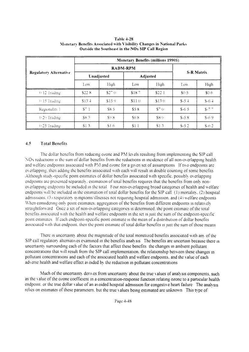
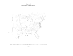 Table 4-28
Monetary Benefits Associated with Visibility Changes in National Parks
Outside the Southeast in the NOx SIP Call Region
Regulatory Alternate e
(' 12 Ira Jini:
('15 "Iradms:
Regionaht\ 1
0 2<> Trading
(i 25 'Irading
Monetan Benefits (millions 1990S)
RADM-RPM
Unadjusted
I. cm
S22 8
S134
S~ 1
$83
SI 3
High
S2"7 0
$159
$85
S9 8
SI 6
Adjusted
Lo\\
$18^
$11 U
$5 8
S68
$1 1
High
S22 1
SI 3(i
S"0
S8 (i
SI 3
S-R Matrix
I,o\\
$05
$-54
$-65
$-58
$-52
High
$06
$-64
$-7"
S-69
$-62
4.5
Total Benefits
The dollar benefits from reducing o/onc and PM le\els resulting from implementing the SIP call
NOx reductions is the sum of dollar benefits from the reductions in incidence of all non-o\erlappmg health
and \\clfare cndpomts associated \\ith PM and o/onc for a an en set of assumptions If t\\o endpomts are
o\erlapping. then adding the benefits associated \\ith each will result in double counting of some benefits
Although studx-specific point estimates of dollar benefits associated \\ith specific, possibh cnerlapping
endpomts are presented separate!}, estimation of total benefits requires that the benefits from onh non-
ox erlapping cndpomts be included in the total Four non-en erlappmg broad categories of health and \\elfare
endpomts \\ill be included in the estimation of total dollar benefits for the SIP call (1) mortality (2) hospital
admissions. (?) respirator) s\mptoms/illnesscs not requiring hospital admission, and (4) \\clfare cndpomts
When considering onh point estimates, aggregation of the benefits from different endpomts is relatneh
straightforward Once a set of non-en erlappmg categories is determined, the point estimate of the total
benefits associated \\ith the health and \\elfare endpomts in the set is just the sum of the endpomt-specific
point estimates If each endpomt-specific point estimate is the mean of a distribution of dollar benefits
associated \\ith that endpomt. then the point estimate of total dollar benefits is ]ust the sum of those means
There is uncertain!} about the magnitude of the total moneti/ed benefits associated \\ith am of the
SIP call regulator) alternate es examined in the benefits anal} sis The benefits are uncertain because there is
uncertamt) surrounding each of the factors that affect these benefits the changes in ambient pollutant
concentrations that \\ill result from the SIP call implementation, the relationship bet\\een these changes in
pollutant concentrations and each of the associated health and welfare endpomts. and the value of each
ad\ erse health and welfare effect a\ oided b> the reduction in pollutant concentrations
Much of the uncertamt} dernes from uncertainty about the true \alues of anal} sis components, such
as the \ alue of the o/one coefficient in a concentration-response function relating ozone to a particular health
endpomt. or the true dollar value of an a\ oided hospital admission for congestive heart failure The analysis
relies on estimates of these parameters, but the true \ alues being estimated are unknown This type of
Page 4-48
image:
Table 4-28
Monetary Benefits Associated with Visibility Changes in National Parks
Outside the Southeast in the NOx SIP Call Region
Regulatory Alternate e
(' 12 Ira Jini:
('15 "Iradms:
Regionaht\ 1
0 2<> Trading
(i 25 'Irading
Monetan Benefits (millions 1990S)
RADM-RPM
Unadjusted
I. cm
S22 8
S134
S~ 1
$83
SI 3
High
S2"7 0
$159
$85
S9 8
SI 6
Adjusted
Lo\\
$18^
$11 U
$5 8
S68
$1 1
High
S22 1
SI 3(i
S"0
S8 (i
SI 3
S-R Matrix
I,o\\
$05
$-54
$-65
$-58
$-52
High
$06
$-64
$-7"
S-69
$-62
4.5
Total Benefits
The dollar benefits from reducing o/onc and PM le\els resulting from implementing the SIP call
NOx reductions is the sum of dollar benefits from the reductions in incidence of all non-o\erlappmg health
and \\clfare cndpomts associated \\ith PM and o/onc for a an en set of assumptions If t\\o endpomts are
o\erlapping. then adding the benefits associated \\ith each will result in double counting of some benefits
Although studx-specific point estimates of dollar benefits associated \\ith specific, possibh cnerlapping
endpomts are presented separate!}, estimation of total benefits requires that the benefits from onh non-
ox erlapping cndpomts be included in the total Four non-en erlappmg broad categories of health and \\elfare
endpomts \\ill be included in the estimation of total dollar benefits for the SIP call (1) mortality (2) hospital
admissions. (?) respirator) s\mptoms/illnesscs not requiring hospital admission, and (4) \\clfare cndpomts
When considering onh point estimates, aggregation of the benefits from different endpomts is relatneh
straightforward Once a set of non-en erlappmg categories is determined, the point estimate of the total
benefits associated \\ith the health and \\elfare endpomts in the set is just the sum of the endpomt-specific
point estimates If each endpomt-specific point estimate is the mean of a distribution of dollar benefits
associated \\ith that endpomt. then the point estimate of total dollar benefits is ]ust the sum of those means
There is uncertain!} about the magnitude of the total moneti/ed benefits associated \\ith am of the
SIP call regulator) alternate es examined in the benefits anal} sis The benefits are uncertain because there is
uncertamt) surrounding each of the factors that affect these benefits the changes in ambient pollutant
concentrations that \\ill result from the SIP call implementation, the relationship bet\\een these changes in
pollutant concentrations and each of the associated health and welfare endpomts. and the value of each
ad\ erse health and welfare effect a\ oided b> the reduction in pollutant concentrations
Much of the uncertamt} dernes from uncertainty about the true \alues of anal} sis components, such
as the \ alue of the o/one coefficient in a concentration-response function relating ozone to a particular health
endpomt. or the true dollar value of an a\ oided hospital admission for congestive heart failure The analysis
relies on estimates of these parameters, but the true \ alues being estimated are unknown This type of
Page 4-48
image:
 uncertain!) can often be quantified For example, the uncertainty about pollutant coefficients is typicalh
quantified b\ reported standard errors of the estimates of the coefficients in the concentration-response
functions estimated b\ epidemiological studies Appendix A presents a formal quantitative anal) sis of the
statistical uncertain!) imparted to the benefits estimates b\ the \ anabihu in the underh ing concentration-
response and valuation functions
Some of the uncertamt) surrounding the results of a benefits anal) sis. howe\er. imohes basicalh
discrete choices and is less easih quantified For example, the decision of \\hich air quality model to use to
generate changes in ambient PM concentrations is a choice between t\\o models, embodying discrete sets of
air chemistn and mathematical assumptions Decisions and assumptions must be made at many points in an
analysis in the absence of complete information The estimate of total benefits is sensitne to the decisions
and assumptions made Among the most critical of these are the following
Ozone mortaliu: There is some uncertain!) surrounding the existence of a relationship betueen
troposphcric o/one exposure and premature mortaht) The two possible assumptions are (1) that
there is no relationship bctuecn o/one and mortaht). and (2) that there is a potential relationship
bet\\cen o/one and mortaht). \\hich \\e can quantif) based on the meta-anahsis of current U S
o/onc mortaht) studies
• Ozone agriculture effects: The existing set of exposure-response functions relating crop yields to
changes in o/.one exposure include both o/one-sensitn c and o/one-msensitn e cultn ars Possible
assumptions are (1) plantings of commodity crop cultn ars are pnmanh composed of sensitne
\aneties. (2) plantings of commodity crop cultn ars are pnmariK composed of non-sensitne
\aneties
PM, 5 concentration threshold: Health effects are measured onh down to the assumed ambient
concentration threshold Changes in air quaht) belo\\ the threshold \\ill ha\ e no impact on estimated
benefits EPA's Science Adxison Board has recommended examining alternatnc thresholds.
including background and 15 ...g'm5
• Sulfate Dominance: There are u\o possible interpretations of PM-related health and \\elfare
benefits depending on the model used to assess air quaht) changes (1) results generated with
RADM-RPM are indicatne of a future eastern L" S atmosphere \\here acid sulfate le\els are still
high enough to control atmospheric chemistn. and more specificalh ammonium nitrate particle
formation In this circumstance, reductions in NOx emissions ma\ result in non-linear responses in
total fine particle le\ els. in\ oh ing both decreases and increases, and (2) results generated with the
Source-Receptor Matrix are indicatne of a future eastern U S. atmosphere where acid sulfate levels
do not dominate particle formation chemistn. In this case, reductions in NOx emissions would be
expected to result more direct!) in linear reductions in PM
• Recreational visibility: Recreational \isibiht) benefits for residents of the Southeast may overlap
with "residential" visibilit) benefits T\\ o alternatn e assumptions may be considered for in-region
residents (1) recreational ^ isibiht) benefits overlap with residential visibility benefits, and to avoid
this o\erlap. the recreational Msibiht) value of $4 per deciview for out-of-region residents is used for
in-region residents ($2 40 for non-indicator parks, and $1 60 for the indicator park), or (2)
recreational visibilit) benefits are in addition to residential visibility benefits, and the m-region \alue
of S6 50 is used (S3 25 for non-indicator parks, and $3 25 for the indicator park)
Page 4-49
image:
uncertain!) can often be quantified For example, the uncertainty about pollutant coefficients is typicalh
quantified b\ reported standard errors of the estimates of the coefficients in the concentration-response
functions estimated b\ epidemiological studies Appendix A presents a formal quantitative anal) sis of the
statistical uncertain!) imparted to the benefits estimates b\ the \ anabihu in the underh ing concentration-
response and valuation functions
Some of the uncertamt) surrounding the results of a benefits anal) sis. howe\er. imohes basicalh
discrete choices and is less easih quantified For example, the decision of \\hich air quality model to use to
generate changes in ambient PM concentrations is a choice between t\\o models, embodying discrete sets of
air chemistn and mathematical assumptions Decisions and assumptions must be made at many points in an
analysis in the absence of complete information The estimate of total benefits is sensitne to the decisions
and assumptions made Among the most critical of these are the following
Ozone mortaliu: There is some uncertain!) surrounding the existence of a relationship betueen
troposphcric o/one exposure and premature mortaht) The two possible assumptions are (1) that
there is no relationship bctuecn o/one and mortaht). and (2) that there is a potential relationship
bet\\cen o/one and mortaht). \\hich \\e can quantif) based on the meta-anahsis of current U S
o/onc mortaht) studies
• Ozone agriculture effects: The existing set of exposure-response functions relating crop yields to
changes in o/.one exposure include both o/one-sensitn c and o/one-msensitn e cultn ars Possible
assumptions are (1) plantings of commodity crop cultn ars are pnmanh composed of sensitne
\aneties. (2) plantings of commodity crop cultn ars are pnmariK composed of non-sensitne
\aneties
PM, 5 concentration threshold: Health effects are measured onh down to the assumed ambient
concentration threshold Changes in air quaht) belo\\ the threshold \\ill ha\ e no impact on estimated
benefits EPA's Science Adxison Board has recommended examining alternatnc thresholds.
including background and 15 ...g'm5
• Sulfate Dominance: There are u\o possible interpretations of PM-related health and \\elfare
benefits depending on the model used to assess air quaht) changes (1) results generated with
RADM-RPM are indicatne of a future eastern L" S atmosphere \\here acid sulfate le\els are still
high enough to control atmospheric chemistn. and more specificalh ammonium nitrate particle
formation In this circumstance, reductions in NOx emissions ma\ result in non-linear responses in
total fine particle le\ els. in\ oh ing both decreases and increases, and (2) results generated with the
Source-Receptor Matrix are indicatne of a future eastern U S. atmosphere where acid sulfate levels
do not dominate particle formation chemistn. In this case, reductions in NOx emissions would be
expected to result more direct!) in linear reductions in PM
• Recreational visibility: Recreational \isibiht) benefits for residents of the Southeast may overlap
with "residential" visibilit) benefits T\\ o alternatn e assumptions may be considered for in-region
residents (1) recreational ^ isibiht) benefits overlap with residential visibility benefits, and to avoid
this o\erlap. the recreational Msibiht) value of $4 per deciview for out-of-region residents is used for
in-region residents ($2 40 for non-indicator parks, and $1 60 for the indicator park), or (2)
recreational visibilit) benefits are in addition to residential visibility benefits, and the m-region \alue
of S6 50 is used (S3 25 for non-indicator parks, and $3 25 for the indicator park)
Page 4-49
image:
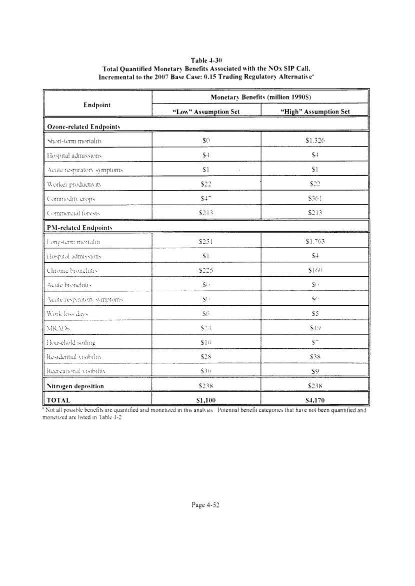
 Benefits from \isibiht\ impro\ements ma\ also occur in N0\ SIP call states outside of the
Southeast The current literature on the \alue of recreational \isibiht> in national parks is limited to
studies of \alucs in California, the Soutrmest. and the Southeast, and thus excludes the Central and
Northeast (CNE) portion of the NOx SIP call region Three altematn e assumptions ma\ be
considered \\hen \aluing \isibiht> changes in the CNE (1) recreational visibility ^ alues in the CNE
are much less than that in the Southeast and therefore to insure benefits are not o\ erstated. no \ alue
should be associated \\ith visibihtx changes in the CNE. (2) recreational \ isibility values in the CNE
are similar to the \ alues for non-indicator parks in the Southeast, and recreational and residential
benefits overlap people in and out of the CNE region \ alue CNE recreational visibility at $2 40 per
decn ie\\. or (?) recreational \ isibihtv \alues in the CNE are similar to the \alues for non-indicator
parks in the Southeast, and there is no overlap of recreational and residential benefits the m-region
CNE \ alue is based on the Southeast m-region \ alue of S3 25 per decn ie\\. and the out-of-region
CNE \ alue is based on the Southeast out-of-region \ alue of S2 40 per decn ie\\
Tables 4-29 through 4-33 present summaries of the endpomt specific monetan \ alues and the
estimate of total benefits for each of the fi\e regulator) altematn es Aggregate results are presented for t\\o
assumption sets 1) a "lo\\" assumption set reflecting the assumptions that human health and the emironment
ha\c lo\\ responsn eness to changes in ambient air quahtv and 2) a "high" assumption set reflecting the
assumptions that human health and the em ironmcnt arc highh responsn e to changes in ambient air quaht\
The "lo\\" assumption set includes the following assumptions 1) there are no PM-related health effects
occurring belo\\ a threshold of 15 jig/m'. 2) changes in PM concentrations are more accurate!} represented b\
the RADM-RPM air quaht> model. 3) there is no relationship betueen o/one and premature mortality. 4)
agricultural commodiK crops are less sensitne to o/one 5) Southeastern recreational \isibilitA \alues are not
transferable to changes in recreational \ isibilit) in the Northeast and Central U S . and 6) the lo\\-end
recreational \ isibilm \ aluation method is correct The "high" assumption set includes the follo\ung
assumptions 1} P\I-related health effects occur down to the anthropogenic background threshold. 2) changes
in PM concentrations are more accuratch represented b> the S-R Matrix air quaht\ model. 3) the relationship
bet\\een o/one and premature mortalit} is characten/ed b\ the distribution of axoided incidences derned
from the o/one mortality meta-anaKsis. 4) agricultural commodit) crops arc more sensitne to o/one. 5)
Southeastern recreational \isibiht\ \alues arc transferable to the Northeastern and Central U S . and 6) the
hiuh-end recreational \isibiht\ method is correct
Page 4-50
image:
Benefits from \isibiht\ impro\ements ma\ also occur in N0\ SIP call states outside of the
Southeast The current literature on the \alue of recreational \isibiht> in national parks is limited to
studies of \alucs in California, the Soutrmest. and the Southeast, and thus excludes the Central and
Northeast (CNE) portion of the NOx SIP call region Three altematn e assumptions ma\ be
considered \\hen \aluing \isibiht> changes in the CNE (1) recreational visibility ^ alues in the CNE
are much less than that in the Southeast and therefore to insure benefits are not o\ erstated. no \ alue
should be associated \\ith visibihtx changes in the CNE. (2) recreational \ isibility values in the CNE
are similar to the \ alues for non-indicator parks in the Southeast, and recreational and residential
benefits overlap people in and out of the CNE region \ alue CNE recreational visibility at $2 40 per
decn ie\\. or (?) recreational \ isibihtv \alues in the CNE are similar to the \alues for non-indicator
parks in the Southeast, and there is no overlap of recreational and residential benefits the m-region
CNE \ alue is based on the Southeast m-region \ alue of S3 25 per decn ie\\. and the out-of-region
CNE \ alue is based on the Southeast out-of-region \ alue of S2 40 per decn ie\\
Tables 4-29 through 4-33 present summaries of the endpomt specific monetan \ alues and the
estimate of total benefits for each of the fi\e regulator) altematn es Aggregate results are presented for t\\o
assumption sets 1) a "lo\\" assumption set reflecting the assumptions that human health and the emironment
ha\c lo\\ responsn eness to changes in ambient air quahtv and 2) a "high" assumption set reflecting the
assumptions that human health and the em ironmcnt arc highh responsn e to changes in ambient air quaht\
The "lo\\" assumption set includes the following assumptions 1) there are no PM-related health effects
occurring belo\\ a threshold of 15 jig/m'. 2) changes in PM concentrations are more accurate!} represented b\
the RADM-RPM air quaht> model. 3) there is no relationship betueen o/one and premature mortality. 4)
agricultural commodiK crops are less sensitne to o/one 5) Southeastern recreational \isibilitA \alues are not
transferable to changes in recreational \ isibilit) in the Northeast and Central U S . and 6) the lo\\-end
recreational \ isibilm \ aluation method is correct The "high" assumption set includes the follo\ung
assumptions 1} P\I-related health effects occur down to the anthropogenic background threshold. 2) changes
in PM concentrations are more accuratch represented b> the S-R Matrix air quaht\ model. 3) the relationship
bet\\een o/one and premature mortalit} is characten/ed b\ the distribution of axoided incidences derned
from the o/one mortality meta-anaKsis. 4) agricultural commodit) crops arc more sensitne to o/one. 5)
Southeastern recreational \isibiht\ \alues arc transferable to the Northeastern and Central U S . and 6) the
hiuh-end recreational \isibiht\ method is correct
Page 4-50
image:
 Table 4-29
Total Quantified Monetan Benefits Associated with the NO\ SIP Call,
Incremental to the 2007 Base Case: 0.12 Trading Regulator} Alternative*
Endpoint
Monetary Benefits (million 1990S)
"Lxnv" Assumption Set
"High" Assumption Set
Ozone-related Endpoints
Short-term moriaht\
Hospital admissions
Acute respirator, sMnptoms
N\ orker products ir\
Commodm crops
Commercial forests
$0
$5
SI
S25
S53
$233
$1.496
$5
SI
$25
S415
$233
PM-related Endpoints
Long-term mortality
Hospital admissions
Chronic bronchitis
Acute bronchi;^
Acute respirators s\mptoms
Woik lo>> da\s
MRADs
1 louschold soiliny:
Residential M>ibiht\
Recieationa! Msihihtx
Nitrogen deposition
TOTAL
SI. 468
S3
S589
S<i
SO
S14
S53
S26
SI IS
S52
S248
S2,888
$2.6^2
$4
$245
S(>
$0
$8
$29
Sll
560
S21
$248
S5,473
* Not all pobiiblc benefits are quantified and monetized in this analxsis Potential benefit categories that ha\e not been quantified anc
monetized are listed in Table 4-2
Page 4-51
image:
Table 4-29
Total Quantified Monetan Benefits Associated with the NO\ SIP Call,
Incremental to the 2007 Base Case: 0.12 Trading Regulator} Alternative*
Endpoint
Monetary Benefits (million 1990S)
"Lxnv" Assumption Set
"High" Assumption Set
Ozone-related Endpoints
Short-term moriaht\
Hospital admissions
Acute respirator, sMnptoms
N\ orker products ir\
Commodm crops
Commercial forests
$0
$5
SI
S25
S53
$233
$1.496
$5
SI
$25
S415
$233
PM-related Endpoints
Long-term mortality
Hospital admissions
Chronic bronchitis
Acute bronchi;^
Acute respirators s\mptoms
Woik lo>> da\s
MRADs
1 louschold soiliny:
Residential M>ibiht\
Recieationa! Msihihtx
Nitrogen deposition
TOTAL
SI. 468
S3
S589
S<i
SO
S14
S53
S26
SI IS
S52
S248
S2,888
$2.6^2
$4
$245
S(>
$0
$8
$29
Sll
560
S21
$248
S5,473
* Not all pobiiblc benefits are quantified and monetized in this analxsis Potential benefit categories that ha\e not been quantified anc
monetized are listed in Table 4-2
Page 4-51
image:
 Table 4-30
Total Quantified Monetan Benefits Associated with the NOx SIP Call,
Incremental to the 2007 Base Case: 0.15 Trading Regulator} Alternate e"
Endpoint
Monetary Benefits (million 1990S)
"Low" Assumption Set
"High" Assumption Set
O/one-related Endpoints
Short-term mortaliu
1 lospita! admission-!
Acute respirators s\rnptoms
X\ orkei products it\
Commodm crops
I ommereid! forests.
$0
$4
SI
$22
S4~
$21?
$1.326
$4
SI
$22
S?6!
S213
PM-related Endpoints
! one-term mo:ulit\
Hospital admissions
Chrome bronchitis
•\cute honchrus
•\ciite lespiraton s\mpioms
Vk'ork loss ja\ s
MRADs
I loiiscliold >oilnij;
Residential \isibili;\
Recieationa! \i.Mbilit\
Nitrogen deposition
TOTAL
S251
SI
S225
S"
SO
S6
S24
Sid
$2*
S30
S2?8
SI, 100
$1.~6?
$4
$160
$i>
Sfl
S5
Siv
s~
S?8
S9
$238
S-4.170
a Not all possible benefits are quantified and moneti/ed in this anahsis Potential benefit categories that ha\e not been quantified and
moncti/ed are listed in Table 4-2
Page 4-52
image:
Table 4-30
Total Quantified Monetan Benefits Associated with the NOx SIP Call,
Incremental to the 2007 Base Case: 0.15 Trading Regulator} Alternate e"
Endpoint
Monetary Benefits (million 1990S)
"Low" Assumption Set
"High" Assumption Set
O/one-related Endpoints
Short-term mortaliu
1 lospita! admission-!
Acute respirators s\rnptoms
X\ orkei products it\
Commodm crops
I ommereid! forests.
$0
$4
SI
$22
S4~
$21?
$1.326
$4
SI
$22
S?6!
S213
PM-related Endpoints
! one-term mo:ulit\
Hospital admissions
Chrome bronchitis
•\cute honchrus
•\ciite lespiraton s\mpioms
Vk'ork loss ja\ s
MRADs
I loiiscliold >oilnij;
Residential \isibili;\
Recieationa! \i.Mbilit\
Nitrogen deposition
TOTAL
S251
SI
S225
S"
SO
S6
S24
Sid
$2*
S30
S2?8
SI, 100
$1.~6?
$4
$160
$i>
Sfl
S5
Siv
s~
S?8
S9
$238
S-4.170
a Not all possible benefits are quantified and moneti/ed in this anahsis Potential benefit categories that ha\e not been quantified and
moncti/ed are listed in Table 4-2
Page 4-52
image:
 Table 4-31
Total Quantified Monetary Benefits Associated with the NOx SIP Call.
Incremental to the 2007 Base Case: Regionally 1 Regulator* Alternate ea
Endpoint
Monetan Benefits (million 1990S)
"Low" Assumption Set
"High" Assumption Set
O/one-related Endpoints
Short-term moriaim
Hospital admissions
Acute respiraton s\mptom.s
\\oiker producmm
C ommoditx crops
Commercial loicsts
$0
$4
$1
$20
S43
SI 88
$1.19.
S4
SI
$2<>
S3 IS
S1HS
PM-related Endpoints
,ont>term monaim
Hospital admissions
Chronic bionchitis
Acute bionch'.lis
•\cuic tespiraion s\mptoms
\\ cirk loss da\ s
MRADs
I iouseh(ilJ -^iilinii
Residential MMhilm
Recicational \ isibi;i;\
Nitrogen deposition
TOTAL
S3 IT
SI
S236
Sd
So
S6
S24
Sin
S?4
S3?
$221
SI, 138
$1.326
$4
$122
SO
$0
S4
$15
$t,
$2"
SK)
$221
S3.45''
1 Not all possible benefits arc quantified and monetized in this anal)sis Potential benefit categories that ha\e not been quantified and
moneti/ed are listed in 1 able 4-2
Page 4-53
image:
Table 4-31
Total Quantified Monetary Benefits Associated with the NOx SIP Call.
Incremental to the 2007 Base Case: Regionally 1 Regulator* Alternate ea
Endpoint
Monetan Benefits (million 1990S)
"Low" Assumption Set
"High" Assumption Set
O/one-related Endpoints
Short-term moriaim
Hospital admissions
Acute respiraton s\mptom.s
\\oiker producmm
C ommoditx crops
Commercial loicsts
$0
$4
$1
$20
S43
SI 88
$1.19.
S4
SI
$2<>
S3 IS
S1HS
PM-related Endpoints
,ont>term monaim
Hospital admissions
Chronic bionchitis
Acute bionch'.lis
•\cuic tespiraion s\mptoms
\\ cirk loss da\ s
MRADs
I iouseh(ilJ -^iilinii
Residential MMhilm
Recicational \ isibi;i;\
Nitrogen deposition
TOTAL
S3 IT
SI
S236
Sd
So
S6
S24
Sin
S?4
S3?
$221
SI, 138
$1.326
$4
$122
SO
$0
S4
$15
$t,
$2"
SK)
$221
S3.45''
1 Not all possible benefits arc quantified and monetized in this anal)sis Potential benefit categories that ha\e not been quantified and
moneti/ed are listed in 1 able 4-2
Page 4-53
image:
 Table 4-32
Total Quantified Monetary Benefits Associated with the NOx SIP Call,
Incremental to the 2007 Base Case: 0.20 Trading Regulatory Alternate e"
Endpoint
Monetary Benefits (million 1990S)
"Low" Assumption Set
"High" Assumption Set
Ozone-related Endpoints
Short-term mortuhn
Hospital admissions
Acute resp;:aton s\mptom>
\\orker product p. in
Commodm crops
Commeicidl lorests
$0
$4
SI
S20
S42
S1S5
$1.108
S4
SI
$2()
S3 12
S185
PM-related Endpoints
I ong-tenr. mor^i'in
1 iospitul admissions
Chionic bionch.Us
•\cutc bronchus
\cuic respnaion v\:r.ptomN
\\ ork loss da\ s
MRADs
I iousehold soilins:
Residential \ iMbilif
Rccreati.'nal \ i^ibn.u
Nitrogen deposition
TOTAL
S3~d
SI
S2 1 6
S'|
S'i
S5
S24
SI"
S?S
S"d
S2 1 0
SI, 156
SI 409
S4
Sl?5
Si '
Sd
S4
sr
$6
S?l
S"
S2 1 0
S3.543
a Not all possible benefits are quantified and moneli/ed in this anaKsis Potential benefit eategones that have not been quantified and
moneti/ed are listed in 1 able 4-2
Page 4-54
image:
Table 4-32
Total Quantified Monetary Benefits Associated with the NOx SIP Call,
Incremental to the 2007 Base Case: 0.20 Trading Regulatory Alternate e"
Endpoint
Monetary Benefits (million 1990S)
"Low" Assumption Set
"High" Assumption Set
Ozone-related Endpoints
Short-term mortuhn
Hospital admissions
Acute resp;:aton s\mptom>
\\orker product p. in
Commodm crops
Commeicidl lorests
$0
$4
SI
S20
S42
S1S5
$1.108
S4
SI
$2()
S3 12
S185
PM-related Endpoints
I ong-tenr. mor^i'in
1 iospitul admissions
Chionic bionch.Us
•\cutc bronchus
\cuic respnaion v\:r.ptomN
\\ ork loss da\ s
MRADs
I iousehold soilins:
Residential \ iMbilif
Rccreati.'nal \ i^ibn.u
Nitrogen deposition
TOTAL
S3~d
SI
S2 1 6
S'|
S'i
S5
S24
SI"
S?S
S"d
S2 1 0
SI, 156
SI 409
S4
Sl?5
Si '
Sd
S4
sr
$6
S?l
S"
S2 1 0
S3.543
a Not all possible benefits are quantified and moneli/ed in this anaKsis Potential benefit eategones that have not been quantified and
moneti/ed are listed in 1 able 4-2
Page 4-54
image:
 Table 4-33
Total Quantified Monetary Benefits Associated with the NO\ SIP Call,
Incremental to the 2007 Base Case: 0.25 Trading Regulatory Alternate ea
Endpoint
Monetary Benefits (million 1990S)
"Low" Assumption Set
"High" Assumption Set
O/one-related Endpoints
Short-term mortalm
Hospital admissions
Acute respirator. s\mptoms
Worker productn it\
C ommodm crops
Commercial forests
$0
S3
SI
S14
S?4
SI 43
S824
$3
SI
$14
S242
$143
PM-related Endpoints
Long-term mortaht\
Hospital admissions
Chronic bronchitis
Acute bronchitis
Acute respiraton s\mptonis
Work loss da\s
MRADS
1 lousehold soiling
Residential \isib:h;\
Recreational Msibihu
Nitrogen deposition
TOTAL
S208
SI
S148
Sc
S"
54
S14
S~
S25
S23
SI 52
S777
SI. 400
S4
S12^
S"
Sd
$4
S16
So
S3d
S5
$152
S2,971
' Not all possible benefits are quantified and monetized in thib analysis Potential benefit categories that ha\e not been quantified and
monetised are listed in Table 4-2
Page 4-55
image:
Table 4-33
Total Quantified Monetary Benefits Associated with the NO\ SIP Call,
Incremental to the 2007 Base Case: 0.25 Trading Regulatory Alternate ea
Endpoint
Monetary Benefits (million 1990S)
"Low" Assumption Set
"High" Assumption Set
O/one-related Endpoints
Short-term mortalm
Hospital admissions
Acute respirator. s\mptoms
Worker productn it\
C ommodm crops
Commercial forests
$0
S3
SI
S14
S?4
SI 43
S824
$3
SI
$14
S242
$143
PM-related Endpoints
Long-term mortaht\
Hospital admissions
Chronic bronchitis
Acute bronchitis
Acute respiraton s\mptonis
Work loss da\s
MRADS
1 lousehold soiling
Residential \isib:h;\
Recreational Msibihu
Nitrogen deposition
TOTAL
S208
SI
S148
Sc
S"
54
S14
S~
S25
S23
SI 52
S777
SI. 400
S4
S12^
S"
Sd
$4
S16
So
S3d
S5
$152
S2,971
' Not all possible benefits are quantified and monetized in thib analysis Potential benefit categories that ha\e not been quantified and
monetised are listed in Table 4-2
Page 4-55
image:
 4.6 Limitations of the Anah sis
Gnen incomplete information, this national benefits anal) sis \iclds approximate results because of
the uncertain!) associated \\ith am estimate Potential!) important sources of uncertain!) exist and mam of
these arc summan/ed in Table 4-34 In most cases, there is no apparent bias associated \\ith the uncertamt)
For those cases for \\hich the nature of the uncertainty suggests a direction of possible bias, this direction is
noted in the table
4.6.1 Projected Income Growth
This anal) sis does not attempt to adjust benefits estimates to reflect expected growth in real income
Economic theon. argues. ho\\e\er. that \VTP for most goods (such as en\ ironmental protection) \\ill increase
if real incomes increase The degree to \\hich \VTP ma) increase for the specific health and \\elfare benefits
pro\ ided b\ the N0\ SIP call cannot be estimated due to insufficient income elasticity information Thus, ail
else being equal, the benefit estimates presented in this anal)sis arc hkeh to be understated
4.6.2 I nquantifiable Benefits
In considering the moneti/ed benefits estimates, the reader should be a\\are that mam limitations for
conducting these anahses are mentioned throughout this RIA One significant limitation of both the health
and \\elfare benefits anahscs is the inabiht) to quantif) mam PM and ozone-induced adxerse effects Table
4-2 lists the categories of benefits that this anal) sis is able to quantif) and those discussed onh in a
qualitatnc manner In general, if it \\cre possible to include the unquantified benefits categories in the total
moncu/ed benefits, the benefits estimates presented in this RIA \\ould increase Specific examples of
unquantified benefits explored in more detail bclo\\ include other human health effects, urban ornamentals.
aesthetic injun to forests, nitrogen in drinking \\ater. and brov,n clouds
The benefits of reductions in a number of o/one- and PM-mduced health effects ha\e not been
quantified due to the una\ ailabiht) of concentration-response and or economic \ aluation data These effects
include reduced pulmonan. function, morphological changes, altered host defense mechanisms, cancer, other
chronic respirator) diseases, infant mortality air\\a\ response eness. increased susceptibihu to respiratory
infection, pulmonar) inflammation, acute inflammation and respirator) cell damage, and premature aging of
the IUITJS
Page 4-56
image:
4.6 Limitations of the Anah sis
Gnen incomplete information, this national benefits anal) sis \iclds approximate results because of
the uncertain!) associated \\ith am estimate Potential!) important sources of uncertain!) exist and mam of
these arc summan/ed in Table 4-34 In most cases, there is no apparent bias associated \\ith the uncertamt)
For those cases for \\hich the nature of the uncertainty suggests a direction of possible bias, this direction is
noted in the table
4.6.1 Projected Income Growth
This anal) sis does not attempt to adjust benefits estimates to reflect expected growth in real income
Economic theon. argues. ho\\e\er. that \VTP for most goods (such as en\ ironmental protection) \\ill increase
if real incomes increase The degree to \\hich \VTP ma) increase for the specific health and \\elfare benefits
pro\ ided b\ the N0\ SIP call cannot be estimated due to insufficient income elasticity information Thus, ail
else being equal, the benefit estimates presented in this anal)sis arc hkeh to be understated
4.6.2 I nquantifiable Benefits
In considering the moneti/ed benefits estimates, the reader should be a\\are that mam limitations for
conducting these anahses are mentioned throughout this RIA One significant limitation of both the health
and \\elfare benefits anahscs is the inabiht) to quantif) mam PM and ozone-induced adxerse effects Table
4-2 lists the categories of benefits that this anal) sis is able to quantif) and those discussed onh in a
qualitatnc manner In general, if it \\cre possible to include the unquantified benefits categories in the total
moncu/ed benefits, the benefits estimates presented in this RIA \\ould increase Specific examples of
unquantified benefits explored in more detail bclo\\ include other human health effects, urban ornamentals.
aesthetic injun to forests, nitrogen in drinking \\ater. and brov,n clouds
The benefits of reductions in a number of o/one- and PM-mduced health effects ha\e not been
quantified due to the una\ ailabiht) of concentration-response and or economic \ aluation data These effects
include reduced pulmonan. function, morphological changes, altered host defense mechanisms, cancer, other
chronic respirator) diseases, infant mortality air\\a\ response eness. increased susceptibihu to respiratory
infection, pulmonar) inflammation, acute inflammation and respirator) cell damage, and premature aging of
the IUITJS
Page 4-56
image:
 Table 4-3-J
Sources of Uncertaint\ in the Benefit Analysis
1. Uncertainties Associated With Concentration-Response Functions
There is uneertamtv surrounding the ozone or PM coefficient in each C-R function
1 here is uncerlamt\ about apphing a single C-R function to pollutant changes and populations in all locations
It is uncertain ho\\ similar future \ear C-R relationships \\ill be to current concentration-response relationships
The correct functional form of each C-R relationship is uncertain For example, it is uncertain \\hether there are
thresholds and. if so \\hat the\ are
There is uncertamn associated \\ilh extrapolation of C-R relationships beyond the range of ozone or PM
concentrations observed in the stud\
2. Uncertainties Associated With Daih Ozone and PM Concentrations
1 here is uncertamn surrounding the protected hourh ozone and daih PM concentrations
1 he changes in ozone and PM concentrations resulting from the SIP call pro\isions are uncertain
3. I ncertainties Associated W ith Possible Lagged Effects
It is uncertain \\hat portion of the PM-related long-term exposure mortality effects associated with changes in annual
PM le\els would occur in a single \ear. and \\hat portion might occur in subsequent \ears
4. Uncertainties Associated With Baseline Incidence Rates
me riasehne incidence rates arc not location-specific (e g . those taken from studies) and ma\ therefore not
accurate!} represent the actual location-specific rates
It is uncertain how well current baseline incidence rates approximate what baseline incidence rales will be in the \ear
2' i(>~ gi\en either "as is" o/one and PM concentrations or am altemame SIP call scenario
It is uncertain how well the proiected population and demographics used to derne incidences, approximate what the
actual population and demographics will be in the \cm 200"
5. Uncertainties Associated With Economic Valuation
Unit dollai \ alue.s associated \vith health and welfare endpomts are onh estimates of MWTP and therefore ha\e
ancertamu surrounding them Possible directions of bias are discussed in the technical support document (Abt
l.\en using constant dollars (e g l'»0 dollars!, it is uncertain whether MWTP for each t\pe of risk i eduction will be
the same in the \ear 20' ~ as the current M\\ 1 P
'I here is uncenainn about the appiopnate discount rate for benefits achie\ ed in the future i200~)
6. U ncertainties Associated W ith Aggregation of Moneti/ed Benefits
Because benefit estimation is limited to those health and welfare endpomts for which concentration-response functions
ha"\e been estimated, there ma\ be components of total benefit omitted This would lead to a downward bias in the
estimated total monetized benefit
Page 4-57
image:
Table 4-3-J
Sources of Uncertaint\ in the Benefit Analysis
1. Uncertainties Associated With Concentration-Response Functions
There is uneertamtv surrounding the ozone or PM coefficient in each C-R function
1 here is uncerlamt\ about apphing a single C-R function to pollutant changes and populations in all locations
It is uncertain ho\\ similar future \ear C-R relationships \\ill be to current concentration-response relationships
The correct functional form of each C-R relationship is uncertain For example, it is uncertain \\hether there are
thresholds and. if so \\hat the\ are
There is uncertamn associated \\ilh extrapolation of C-R relationships beyond the range of ozone or PM
concentrations observed in the stud\
2. Uncertainties Associated With Daih Ozone and PM Concentrations
1 here is uncertamn surrounding the protected hourh ozone and daih PM concentrations
1 he changes in ozone and PM concentrations resulting from the SIP call pro\isions are uncertain
3. I ncertainties Associated W ith Possible Lagged Effects
It is uncertain \\hat portion of the PM-related long-term exposure mortality effects associated with changes in annual
PM le\els would occur in a single \ear. and \\hat portion might occur in subsequent \ears
4. Uncertainties Associated With Baseline Incidence Rates
me riasehne incidence rates arc not location-specific (e g . those taken from studies) and ma\ therefore not
accurate!} represent the actual location-specific rates
It is uncertain how well current baseline incidence rates approximate what baseline incidence rales will be in the \ear
2' i(>~ gi\en either "as is" o/one and PM concentrations or am altemame SIP call scenario
It is uncertain how well the proiected population and demographics used to derne incidences, approximate what the
actual population and demographics will be in the \cm 200"
5. Uncertainties Associated With Economic Valuation
Unit dollai \ alue.s associated \vith health and welfare endpomts are onh estimates of MWTP and therefore ha\e
ancertamu surrounding them Possible directions of bias are discussed in the technical support document (Abt
l.\en using constant dollars (e g l'»0 dollars!, it is uncertain whether MWTP for each t\pe of risk i eduction will be
the same in the \ear 20' ~ as the current M\\ 1 P
'I here is uncenainn about the appiopnate discount rate for benefits achie\ ed in the future i200~)
6. U ncertainties Associated W ith Aggregation of Moneti/ed Benefits
Because benefit estimation is limited to those health and welfare endpomts for which concentration-response functions
ha"\e been estimated, there ma\ be components of total benefit omitted This would lead to a downward bias in the
estimated total monetized benefit
Page 4-57
image:
 In addition to the abo\c non-moncti/ed health benefits, there are a number of non-monetized \\elfare
benefits of NO\ emission controls from reduced ad\erse effects on \egetation. forests, and other natural
CCOSN stems The CAA and other statutes, through requirements to protect natural and ecological s> stems.
indicate that these are scarce and highh \ alued resources Lack of comprehcnsn e information, insufficient
\ aluation tools, and significant uncertainties result in understated \\elfare benefits estimates in this R1A
Ho\\e\cr. a number of expert biologists, ecologists. and economists (Costanza. 1997) argue that the benefits
of protecting natural resources are enormous and increasing as ecos> stems become more stressed and scarce
in the future Additional!}.. agricultural, forest and ecological scientists (Heck. 1997) believe that v egetation
appears to be more sensitn e to ozone than humans and consequent!}. that damage is occurring to \ egetation
and natural resources at concentrations below the ozone N AAQS Experts also belie\ e that the effect of
ozone on plants is both cumulame and long-term The specific non-monetized benefits from reductions in
ambient ozone concentrations \\ould accrue from decreased foliar injun . a\erted growth reduction of trees in
natural forests, maintained integrity of forest ecos\ stems (including habitat for name animal species), and
the aesthetics and utilit> of urban ornamentals (e g . grass, flowers, shrubs and trees) Other welfare
categories for \\hich there is incomplete information to estimate the economic \alue of reduced adverse
effects include existence value of Class 1 areas, materials damage, reduced sulfate deposition to aquatic and
terrestrial ecos\ stems, and usibihu impairment due to "brown clouds" (i e . distinct brown lasers of trapped
air pollutants close to the ground)
Other Human Health Effects
Human exposure to PM and ozone is known to cause health effects such as airwa\ response eness.
increased susceptibility to respirator, infection, acute inflammation and respirator, cell damage, premature
aging of the lungs and chronic respirator, damage An impro\ement in ambient PM and ozone air quality is
expected to reduce the number of incidences \\ithm each effect categon that the U S population \\ould
experience Although these health effects are kno\\n to be PM or ozone-induced, concentration-response data
is not a\ ailablc for quantising the benefits associated \\ith reducing these effects The mabiht\ to quantify
these effects leads to an underestimation of the monetized benefits presented in this anaKsis
I rban Ornamentals
Urban ornamentals represent an additional \egetation categor. hkeh to experience some degree of
effects associated \\ith exposure to ambient ozone le\els and hkeK to impact large economic sectors In the
absence of adequate exposure-response functions and economic damage functions for the potential range of
effects rele\ ant to these r\pcs of •<. egetation. no direct quantitati\e economic benefits anaKsis has been
conducted Ornamentals used in the urban and suburban landscape include shrubs, trees, grasses, and
flowers The t\pes of economic losses that could potential!} result from effects that ha\e been associated
with ozone exposure include 1) reduction in aesthetic sen ices o\er the realized lifetime of a plant. 2) the loss
of aesthetic sen ices resulting from the premature death (or earK replacement) of an injured plant. 3) the cost
associated \\ith remo\mg the injured plant and replacing it \\ith a ne\\ plant. 4) increased soil erosion. 5)
increased energy costs from loss of shade in the urban emironment. 6) reduced seedling sunn ability, and 7)
am additional costs incurred o\er the lifetime of the injured plant to mitigate the effects of ozone-induced
injun It is estimated that more than $20 billion (1990 dollars) are spent annually on landscaping using
ornamentals (Abt Associates. 1995). both b\ private property owners/tenants and b> governmental units
responsible for public areas, making this a potential!}, important \\elfare effects categon. However.
information and valuation methods are not a\ ailable to allow for plausible estimates of the percentage of
these expenditures that may be related to impacts associated with ozone exposure
Page 4-58
image:
In addition to the abo\c non-moncti/ed health benefits, there are a number of non-monetized \\elfare
benefits of NO\ emission controls from reduced ad\erse effects on \egetation. forests, and other natural
CCOSN stems The CAA and other statutes, through requirements to protect natural and ecological s> stems.
indicate that these are scarce and highh \ alued resources Lack of comprehcnsn e information, insufficient
\ aluation tools, and significant uncertainties result in understated \\elfare benefits estimates in this R1A
Ho\\e\cr. a number of expert biologists, ecologists. and economists (Costanza. 1997) argue that the benefits
of protecting natural resources are enormous and increasing as ecos> stems become more stressed and scarce
in the future Additional!}.. agricultural, forest and ecological scientists (Heck. 1997) believe that v egetation
appears to be more sensitn e to ozone than humans and consequent!}. that damage is occurring to \ egetation
and natural resources at concentrations below the ozone N AAQS Experts also belie\ e that the effect of
ozone on plants is both cumulame and long-term The specific non-monetized benefits from reductions in
ambient ozone concentrations \\ould accrue from decreased foliar injun . a\erted growth reduction of trees in
natural forests, maintained integrity of forest ecos\ stems (including habitat for name animal species), and
the aesthetics and utilit> of urban ornamentals (e g . grass, flowers, shrubs and trees) Other welfare
categories for \\hich there is incomplete information to estimate the economic \alue of reduced adverse
effects include existence value of Class 1 areas, materials damage, reduced sulfate deposition to aquatic and
terrestrial ecos\ stems, and usibihu impairment due to "brown clouds" (i e . distinct brown lasers of trapped
air pollutants close to the ground)
Other Human Health Effects
Human exposure to PM and ozone is known to cause health effects such as airwa\ response eness.
increased susceptibility to respirator, infection, acute inflammation and respirator, cell damage, premature
aging of the lungs and chronic respirator, damage An impro\ement in ambient PM and ozone air quality is
expected to reduce the number of incidences \\ithm each effect categon that the U S population \\ould
experience Although these health effects are kno\\n to be PM or ozone-induced, concentration-response data
is not a\ ailablc for quantising the benefits associated \\ith reducing these effects The mabiht\ to quantify
these effects leads to an underestimation of the monetized benefits presented in this anaKsis
I rban Ornamentals
Urban ornamentals represent an additional \egetation categor. hkeh to experience some degree of
effects associated \\ith exposure to ambient ozone le\els and hkeK to impact large economic sectors In the
absence of adequate exposure-response functions and economic damage functions for the potential range of
effects rele\ ant to these r\pcs of •<. egetation. no direct quantitati\e economic benefits anaKsis has been
conducted Ornamentals used in the urban and suburban landscape include shrubs, trees, grasses, and
flowers The t\pes of economic losses that could potential!} result from effects that ha\e been associated
with ozone exposure include 1) reduction in aesthetic sen ices o\er the realized lifetime of a plant. 2) the loss
of aesthetic sen ices resulting from the premature death (or earK replacement) of an injured plant. 3) the cost
associated \\ith remo\mg the injured plant and replacing it \\ith a ne\\ plant. 4) increased soil erosion. 5)
increased energy costs from loss of shade in the urban emironment. 6) reduced seedling sunn ability, and 7)
am additional costs incurred o\er the lifetime of the injured plant to mitigate the effects of ozone-induced
injun It is estimated that more than $20 billion (1990 dollars) are spent annually on landscaping using
ornamentals (Abt Associates. 1995). both b\ private property owners/tenants and b> governmental units
responsible for public areas, making this a potential!}, important \\elfare effects categon. However.
information and valuation methods are not a\ ailable to allow for plausible estimates of the percentage of
these expenditures that may be related to impacts associated with ozone exposure
Page 4-58
image:
 Aesthetic Injury to Forests
O/one is a regional!) dispersed air pollutant that has been sho\\n conclusive!) to cause discernible
to forest trees (Fox. 1995) One of the \\clfare benefits expected to accrue as a result of reductions in
ambient o/onc concentrations in the United States is the economic \ alue the public receives from reduced
aesthetic m]ur> to forests There is sufficient scientific information available that ambient ozone le\ els cause
visible miun to foliage and impair the growth of some sensitn e plant species Ozone inhibits photos\nthesis
and interferes with nutrient uptake, causing a loss in \ igor that affects the abiht> of trees to compete for
resources and makes them more susceptible to a \ anety of stresses (EPA. 1996a. p 5-251) Extended or
repeated exposures ma\ result in decline and e\ entual elimination of sensitn e species Ozone concentrations
of 0 06 ppm or higher arc capable of causing injun to forest ecos\ stems
The most notable effects of ozone on forest aesthetics and ecosystem function ha\e been documented
in the San Bernardino Mountains in California Visible ozone-related injun. but not necessanh ecosvstem
effects. ha\ e also been obsen ed in the Sierra Ne\ ada in California, the Appalachian Mountains from
Georma to Maine, the Blue Ridge Mountains in Virginia, the Great Smoky Mountains in North Carolina and
Tennessee, and the Green Mountains in Vermont (EPA. 1996a. pp 5-250 to 5-251) These are all locations
\\here there is substantial recreation use and \\here scenic quaht) of the forests is an important characteristic
of the resource Economic \ aluation studies of lost aesthetic value of forests attributed to plant injuries
caused b\ o/onc arc limited to t\\o studies conducted in Southern California (Crocker. 1985. Peterson et al .
1987) Both included contingent \ aluation sun e> s that asked respondents \\hat the> \\ould be \\ illmg to pa>
for reductions in (or prc\ entions of increases in) •*, isible ozone injuries to plants Crocker found that
indniduals are \\illmg to pa\ a fe\\ dollars more per da> to gain access to recreation areas \Mth onh slight
o/one miun instead of areas \vith moderate to se\ere injun Peterson et al estimated that a one-step change
(on a 5 point scale) in \ isible ozone injun in the San Bernardino and Angeles National Forests \\ould be
\alued at an aggregate amount of between S27 million and SI 44 million for all residents of Los Angeles.
Orange, and San Bernardino counties A reassessment of the sune\ design, in light of current standards for
contingent \ aluation research, suggests that it is plausible that concerns for forest ecosx stems and human
health could ha\c been embedded into these reported \ alues The extent of this possible bias is uncertain
Present anahtic tools and resources preclude EPA from quantifying the benefits of impro\ed forest
aesthetics in the eastern U S expected to occur from the NOx SIP call This is due to limitations in our
abiht} to quantifx the relationship between ozone concentrations and \ isible mjun. and limited quantitatn e
information about the \alue to the public of specific changes in \isible aesthetic quality of forests Hov\e\er.
there is sufficient supporting e\ idence in the ph\ sical sciences and economic literature to support the finding
that the proposed NOx SIP call can be expected to reduce mjun to forests, and that reductions in these
miunes \\ill likeK ha\e a significant economic \alue to the public
Nitrates in Drinking Water
Nitrates in drinking water are currenth regulated b\ a maximum contaminant level (MCL) of 10
mg/L on the basis of the risk to infants of methemoglobinemia. a condition which ad^ersel\• affects the
blood's ox>gen cam-mg capacity In an analysis of pre-1991 data. Raucher. et al (1993) found that
approximately 2 million people were consuming public drinking water supplies which exceed the MCL
Supplementing these findings, the National Research Council concluded that 42 percent of the public
drinking water users in the U S (approximately 105 million people) are either not exposed to nitrates or are
exposed to concentrations below 1 3 mg/L (National Research Council. 1995)
Page 4-59
image:
Aesthetic Injury to Forests
O/one is a regional!) dispersed air pollutant that has been sho\\n conclusive!) to cause discernible
to forest trees (Fox. 1995) One of the \\clfare benefits expected to accrue as a result of reductions in
ambient o/onc concentrations in the United States is the economic \ alue the public receives from reduced
aesthetic m]ur> to forests There is sufficient scientific information available that ambient ozone le\ els cause
visible miun to foliage and impair the growth of some sensitn e plant species Ozone inhibits photos\nthesis
and interferes with nutrient uptake, causing a loss in \ igor that affects the abiht> of trees to compete for
resources and makes them more susceptible to a \ anety of stresses (EPA. 1996a. p 5-251) Extended or
repeated exposures ma\ result in decline and e\ entual elimination of sensitn e species Ozone concentrations
of 0 06 ppm or higher arc capable of causing injun to forest ecos\ stems
The most notable effects of ozone on forest aesthetics and ecosystem function ha\e been documented
in the San Bernardino Mountains in California Visible ozone-related injun. but not necessanh ecosvstem
effects. ha\ e also been obsen ed in the Sierra Ne\ ada in California, the Appalachian Mountains from
Georma to Maine, the Blue Ridge Mountains in Virginia, the Great Smoky Mountains in North Carolina and
Tennessee, and the Green Mountains in Vermont (EPA. 1996a. pp 5-250 to 5-251) These are all locations
\\here there is substantial recreation use and \\here scenic quaht) of the forests is an important characteristic
of the resource Economic \ aluation studies of lost aesthetic value of forests attributed to plant injuries
caused b\ o/onc arc limited to t\\o studies conducted in Southern California (Crocker. 1985. Peterson et al .
1987) Both included contingent \ aluation sun e> s that asked respondents \\hat the> \\ould be \\ illmg to pa>
for reductions in (or prc\ entions of increases in) •*, isible ozone injuries to plants Crocker found that
indniduals are \\illmg to pa\ a fe\\ dollars more per da> to gain access to recreation areas \Mth onh slight
o/one miun instead of areas \vith moderate to se\ere injun Peterson et al estimated that a one-step change
(on a 5 point scale) in \ isible ozone injun in the San Bernardino and Angeles National Forests \\ould be
\alued at an aggregate amount of between S27 million and SI 44 million for all residents of Los Angeles.
Orange, and San Bernardino counties A reassessment of the sune\ design, in light of current standards for
contingent \ aluation research, suggests that it is plausible that concerns for forest ecosx stems and human
health could ha\c been embedded into these reported \ alues The extent of this possible bias is uncertain
Present anahtic tools and resources preclude EPA from quantifying the benefits of impro\ed forest
aesthetics in the eastern U S expected to occur from the NOx SIP call This is due to limitations in our
abiht} to quantifx the relationship between ozone concentrations and \ isible mjun. and limited quantitatn e
information about the \alue to the public of specific changes in \isible aesthetic quality of forests Hov\e\er.
there is sufficient supporting e\ idence in the ph\ sical sciences and economic literature to support the finding
that the proposed NOx SIP call can be expected to reduce mjun to forests, and that reductions in these
miunes \\ill likeK ha\e a significant economic \alue to the public
Nitrates in Drinking Water
Nitrates in drinking water are currenth regulated b\ a maximum contaminant level (MCL) of 10
mg/L on the basis of the risk to infants of methemoglobinemia. a condition which ad^ersel\• affects the
blood's ox>gen cam-mg capacity In an analysis of pre-1991 data. Raucher. et al (1993) found that
approximately 2 million people were consuming public drinking water supplies which exceed the MCL
Supplementing these findings, the National Research Council concluded that 42 percent of the public
drinking water users in the U S (approximately 105 million people) are either not exposed to nitrates or are
exposed to concentrations below 1 3 mg/L (National Research Council. 1995)
Page 4-59
image:
 In a recent cpidemiological stuch b\ the National Cancer Institute, a statistical!) significant
relationship bet\\ccn nitrates in drinking \\ater and incidence of non-Hodgkin's lymphoma \\ere reported
(\\ ard. et al . 1996) Though it is generalh acknowledged that traditional water pollution sources such as
agricultural runoff are mosth responsible for \iolations of the MCL. other more diffuse sources of nitrate to
drinking \\ater supplies, such as that from atmospheric deposition. ma> also become an important health
concern should the cancer link to nitrates be found \ ahd upon further study
Brown Clouds
NOx emissions, especially gaseous NCK and NO\ aerosols, can cause a brownish color to appear in
the air (EPA. 1996c) In higher elexation \\estern cities \\here wintertime temperature imersions frequently
trap air pollutants in atmospheric layers close to the ground, this can result in distinct brown la> ers In the
eastern L S . a la\ered look is not as common, but the ubiquitous haze sometimes takes on a brownish hue
To date, economic \aluation studies concerning visual air quahtx ha\e focused primanh on the clant> of the
air. and ha\c not addressed the question of ho\\ the color of the ha/e might be related to aesthetic
degradation It ma> be reasonable to presume that brown ha/e is hkeh to be perceived as dirt> air and is
more hkeh to be associated \\ith air pollution in people's minds It has not. ho\\e\er. been established that
the public \\ould hax e a greater \ alue for reducing bro\\n ha/e than for a neutral colored ha/c Results of
economic \ aluation studies of x isibihh aesthetics conducted in Dem er and in the eastern U S (McClelland
ct al . 199] i are not directh comparable because changes in \isibiht> conditions are not defined in the same
units of measure Ho\\e\cr. the \VTP estimates for impro\ements in \isibiht> conditions presented in this
assessment are based on estimates of changes in clanu of the air (measured as deciMC\\) and do not take into
account am change in color that ma\ occur It is possible that there ma> be some additional \ alue for
reductions in bro\\msh color that max also occur \\hcn N0\ emissions are reduced
Other I nquantifiable Benefits Categories
There are other \\elfarc benefits categories for \\hich there is incomplete information to permit a
quantnatn e assessment for this anah sis For some endpomts. gaps exist in the scientific literature or ke>
anahlical components and thus do not support an estimation of incidence In other cases, there is insufficient
economic information to allo\\ estimation of the economic x alue of ad\ ersc effects Potential!} significant.
but unquantified \\clfarc benefits categories include existence and user x alues related to the protection of
Class 1 areas (e g . Shenendoah National Park), damage to tree seedlings of more than 10 sensitne species
(e g . black cherry aspen, ponderosa pinej. non-commercial forests, ecosx stems, materials damage, and
reduced sulfate deposition to aquatic and terrestrial ecos\ stems Although scientific and economic data are
not axailablc to allo\\ quantification of the effect of o/one in these categories, the expectation is that, if
quantified, each of these categories \\ould lead to an increase in the moneti/ed benefits presented in this RIA
4.6.3 Potential Disbenefits
In this discussion of unquantified benefits, a discussion of potential disbenefits must also be
mentioned Se\ eral of these disbenefit categories are related to nitrogen deposition while one category is
related to the issue of ultraMolet light
Page 4-60
image:
In a recent cpidemiological stuch b\ the National Cancer Institute, a statistical!) significant
relationship bet\\ccn nitrates in drinking \\ater and incidence of non-Hodgkin's lymphoma \\ere reported
(\\ ard. et al . 1996) Though it is generalh acknowledged that traditional water pollution sources such as
agricultural runoff are mosth responsible for \iolations of the MCL. other more diffuse sources of nitrate to
drinking \\ater supplies, such as that from atmospheric deposition. ma> also become an important health
concern should the cancer link to nitrates be found \ ahd upon further study
Brown Clouds
NOx emissions, especially gaseous NCK and NO\ aerosols, can cause a brownish color to appear in
the air (EPA. 1996c) In higher elexation \\estern cities \\here wintertime temperature imersions frequently
trap air pollutants in atmospheric layers close to the ground, this can result in distinct brown la> ers In the
eastern L S . a la\ered look is not as common, but the ubiquitous haze sometimes takes on a brownish hue
To date, economic \aluation studies concerning visual air quahtx ha\e focused primanh on the clant> of the
air. and ha\c not addressed the question of ho\\ the color of the ha/e might be related to aesthetic
degradation It ma> be reasonable to presume that brown ha/e is hkeh to be perceived as dirt> air and is
more hkeh to be associated \\ith air pollution in people's minds It has not. ho\\e\er. been established that
the public \\ould hax e a greater \ alue for reducing bro\\n ha/e than for a neutral colored ha/c Results of
economic \ aluation studies of x isibihh aesthetics conducted in Dem er and in the eastern U S (McClelland
ct al . 199] i are not directh comparable because changes in \isibiht> conditions are not defined in the same
units of measure Ho\\e\cr. the \VTP estimates for impro\ements in \isibiht> conditions presented in this
assessment are based on estimates of changes in clanu of the air (measured as deciMC\\) and do not take into
account am change in color that ma\ occur It is possible that there ma> be some additional \ alue for
reductions in bro\\msh color that max also occur \\hcn N0\ emissions are reduced
Other I nquantifiable Benefits Categories
There are other \\elfarc benefits categories for \\hich there is incomplete information to permit a
quantnatn e assessment for this anah sis For some endpomts. gaps exist in the scientific literature or ke>
anahlical components and thus do not support an estimation of incidence In other cases, there is insufficient
economic information to allo\\ estimation of the economic x alue of ad\ ersc effects Potential!} significant.
but unquantified \\clfarc benefits categories include existence and user x alues related to the protection of
Class 1 areas (e g . Shenendoah National Park), damage to tree seedlings of more than 10 sensitne species
(e g . black cherry aspen, ponderosa pinej. non-commercial forests, ecosx stems, materials damage, and
reduced sulfate deposition to aquatic and terrestrial ecos\ stems Although scientific and economic data are
not axailablc to allo\\ quantification of the effect of o/one in these categories, the expectation is that, if
quantified, each of these categories \\ould lead to an increase in the moneti/ed benefits presented in this RIA
4.6.3 Potential Disbenefits
In this discussion of unquantified benefits, a discussion of potential disbenefits must also be
mentioned Se\ eral of these disbenefit categories are related to nitrogen deposition while one category is
related to the issue of ultraMolet light
Page 4-60
image:
 Passive Fertilization
Sc\ eral disbencfit categories are related to nitrogen deposition Nutrients deposited on crops from
atmospheric sources are often referred to as passn e fertilization Nitrogen is a fundamental nutrient for
pnman production in both managed and unmanaged ecos> stems Most producm e agricultural s\ stems
require external sources of nitrogen in order to satisfy nutrient requirements Nitrogen uptake b\ crops
\aries. but t\pical requirements for \\heat and corn are approximate!) 150 kg/ha/yr and 300 kg/ha/yr.
respecm el\ (N APAP. 1990) These rates compare to estimated rates of passive nitrogen fertilization in the
range of 0 to 5 5 kg/haVr (NAPAP. 1991) So. for these crops, deposited nitrogen could account for as much
as 2 to 4 percent of nitrogen needs Holding all other factors constant, farmers" use of purchased fertilizers or
manure ma\ increase as deposited nitrogen is reduced EPA has not estimated the potential A alue of this
possible increase in the use of purchased fertilizers, but a quahtatne assessment of several factors suggests
that the o\ erali \ alue is \ en small relam e to the \ alue of other health and welfare endpomts presented in this
anah sis First, reductions in N'0\ emissions affect onl\ a fraction of total nitrogen deposition
Approximate!) 70 to 80 percent of nitrogen deposition is in the form of nitrates (and thus can be traced to
N0\ emissions) \vhile most of the remainder is due to ammonia emissions (personal communication \\ith
Robin Dennis. NOAA Atmospheric Research Lab. 1997) Table 3-4 in Chapter 3 indicates the annual
a\erage change in nitrogen deposition attributable to the 0 15 Trading alternatne of the N0\ SIP call is
about 11 percent of baseline le\els. suggesting a relatneh small potential change in passn e fertilization
Second, some sources of nitrogen, such as animal manure, are a\ ailable at no cost or at a much lo\\er cost
than purchased nitrogen In addition, in certain areas nitrogen is current!) applied at rates \\hich exceed crop
uptake rates, usualh due to an o\ erabundance of a\ ailable nutrients from animal waste Small reductions in
passive fertilization in these areas is not hkeh to ha\e am consequence to fertilizer application The
combination of these factors suggests that the cost associated \\ith compensating for reductions in passn e
fertih/ation is rclatnel) minor
Information on the effects of changes in passn c nitrogen deposition on forestlands and other
terrestrial ecos\ stems is \er\ limited The multiplicity of factors affecting forests, including other potential
stressors such as ozone, and limiting factors such as moisture and other nutrients, confound assessments of
marginal changes in am one stressor or nutrient in forest ecos\ stems Ho\\e\ er. reductions in deposition of
nitrogen could ha\e ncgatne effects on forest and \egetation growth in ecos> stems \\hcre nitrogen is a
limiting factor (EPA. 1993)
On the other hand, there is CMdence that forest ecos> stems in some areas of the United States are
nitrogen saturated (EPA. 1993) Once saturation is reached. ad\erse effects of additional nitrogen begin to
occur such as soil acidification which can lead to leaching of nutrients needed for plant growth and
mobilization of harmful elements such as aluminum Increased soil acidification is also linked to higher
amounts of acidic runoff to streams and lakes and leaching of harmful elements into aquatic ecos> stems
Ultraviolet Light
A reduction of troposphenc ozone is likely to increase the penetration of ultraviolet light, specificalh
UV-b. to ground le\el UV-b is an issue of concern because depletion of the stratospheric ozone layer (i e ,
ozone in the upper atmosphere) due to chlorofluorocarbons and other ozone-depleting chemicals is associated
with increased skin cancer and cataract rates Currenth. EPA is not able to adequately quantify these effects
for the purpose of \ alumg benefits for this pohc>
Page 4-61
image:
Passive Fertilization
Sc\ eral disbencfit categories are related to nitrogen deposition Nutrients deposited on crops from
atmospheric sources are often referred to as passn e fertilization Nitrogen is a fundamental nutrient for
pnman production in both managed and unmanaged ecos> stems Most producm e agricultural s\ stems
require external sources of nitrogen in order to satisfy nutrient requirements Nitrogen uptake b\ crops
\aries. but t\pical requirements for \\heat and corn are approximate!) 150 kg/ha/yr and 300 kg/ha/yr.
respecm el\ (N APAP. 1990) These rates compare to estimated rates of passive nitrogen fertilization in the
range of 0 to 5 5 kg/haVr (NAPAP. 1991) So. for these crops, deposited nitrogen could account for as much
as 2 to 4 percent of nitrogen needs Holding all other factors constant, farmers" use of purchased fertilizers or
manure ma\ increase as deposited nitrogen is reduced EPA has not estimated the potential A alue of this
possible increase in the use of purchased fertilizers, but a quahtatne assessment of several factors suggests
that the o\ erali \ alue is \ en small relam e to the \ alue of other health and welfare endpomts presented in this
anah sis First, reductions in N'0\ emissions affect onl\ a fraction of total nitrogen deposition
Approximate!) 70 to 80 percent of nitrogen deposition is in the form of nitrates (and thus can be traced to
N0\ emissions) \vhile most of the remainder is due to ammonia emissions (personal communication \\ith
Robin Dennis. NOAA Atmospheric Research Lab. 1997) Table 3-4 in Chapter 3 indicates the annual
a\erage change in nitrogen deposition attributable to the 0 15 Trading alternatne of the N0\ SIP call is
about 11 percent of baseline le\els. suggesting a relatneh small potential change in passn e fertilization
Second, some sources of nitrogen, such as animal manure, are a\ ailable at no cost or at a much lo\\er cost
than purchased nitrogen In addition, in certain areas nitrogen is current!) applied at rates \\hich exceed crop
uptake rates, usualh due to an o\ erabundance of a\ ailable nutrients from animal waste Small reductions in
passive fertilization in these areas is not hkeh to ha\e am consequence to fertilizer application The
combination of these factors suggests that the cost associated \\ith compensating for reductions in passn e
fertih/ation is rclatnel) minor
Information on the effects of changes in passn c nitrogen deposition on forestlands and other
terrestrial ecos\ stems is \er\ limited The multiplicity of factors affecting forests, including other potential
stressors such as ozone, and limiting factors such as moisture and other nutrients, confound assessments of
marginal changes in am one stressor or nutrient in forest ecos\ stems Ho\\e\ er. reductions in deposition of
nitrogen could ha\e ncgatne effects on forest and \egetation growth in ecos> stems \\hcre nitrogen is a
limiting factor (EPA. 1993)
On the other hand, there is CMdence that forest ecos> stems in some areas of the United States are
nitrogen saturated (EPA. 1993) Once saturation is reached. ad\erse effects of additional nitrogen begin to
occur such as soil acidification which can lead to leaching of nutrients needed for plant growth and
mobilization of harmful elements such as aluminum Increased soil acidification is also linked to higher
amounts of acidic runoff to streams and lakes and leaching of harmful elements into aquatic ecos> stems
Ultraviolet Light
A reduction of troposphenc ozone is likely to increase the penetration of ultraviolet light, specificalh
UV-b. to ground le\el UV-b is an issue of concern because depletion of the stratospheric ozone layer (i e ,
ozone in the upper atmosphere) due to chlorofluorocarbons and other ozone-depleting chemicals is associated
with increased skin cancer and cataract rates Currenth. EPA is not able to adequately quantify these effects
for the purpose of \ alumg benefits for this pohc>
Page 4-61
image:
 Other EPA programs exist to address the risks posed b\ changes in UV-b associated \\ith changes in
total column o/one As presented in the Stratospheric Ozone RIA (EPA. 1992). stratospheric ozone le\els
are expected to significant!) improxe o\er the next centun as the major ozone depleting substances are
phased out globalh This expected impro\ ement in stratospheric ozone le\ els is estimated to reduce the
number of nonmelanoma skin cancers (NMSC's) b> millions of cases in the U S b> 2075
4.7 References
Abt Associates. Inc 1992 The Medical Costs of Five Illnesses Related to Exposure to Pollutants
Prepared for the U S Em ironmcntal Protection Agencv Office of Pollution Pre\cntion and Toxics.
Washington. DC
Abt Associates. Inc 1995 I'rhan Ornamental Plants Sensitivity to Ozone and Potential Economic Losses
Prepared for the L' S Em ironmental Protection Agencv Office of Air QualiU Planning and Standards.
Research Triangle Park. \ C . Jul\
Abt Associates. Inc 1998a Selectee/Health and Wei/are Benefits Methods for the NOx SIP Call RIA.
Prepared for the U S Em ironmcntal Protection Agenc>. Office of Air Quaht> Planning and
Standards. Research Triangle Park. N C . September
Abt Associates Inc 1998b Agricultural Benefits I'.sing AGSIM for the .\()x SIP Call Draft Report
Prepared for the I S Em ironmental Protection Agencv Office of Air Quality Planning and Standards.
Research Triangle Park. N C . September
Chestnut. L 1997 Draft Memorandum .\fethodoiog\ for Estimating I'alues for Changes in 1'isihihtvat
National ParL\ (April 15)
Costanza. R . d'Arge. R . de Groot. R . Farber. S . Grasso. M . Hannon. B . Limburg. K. Naeem. S . O'Neill.
R V . Paruelo. J . Raskin. R G . Sutton. P . and \an den Belt. M (1997). The Value of the \Vorld~sEcos\stcm
Scnices and Natural Capital Mature. Yol 387 253-259
Crocker T D . Horst R L . Jr 1981 Hours of Work. Labor Producm it\. and Em ironmental Conditions a
Case Stud\ Jne Revie\\ ol Economics and Statistics 63 361-368
Crocker. T D (1985 ). On the Value of the Condition of a Forest Stock Land Economics 61(3) 244-254
Cropper. M L and A J Krupmck 1990 The Social Costs of Chronic Heart and Lung Disease Resources
for the Future Discussion Paper QE 89-16-REY
Cummmgs. R . H Burness and R Norton 1981 Methods Development for Environmental Control
Benefits Assessment. Volume V Measuring Household Soiling Damages from Suspended Air Particulatcs..
A Methodological Inquirv Report prepared for the U S Environmental Protection Agenc>. Washington.
DC
Dennis. R 1998 Personal communication NOAA Atmospheric Research Lab. Research Triangle Park.
N C . August 31
Page 4-62
image:
Other EPA programs exist to address the risks posed b\ changes in UV-b associated \\ith changes in
total column o/one As presented in the Stratospheric Ozone RIA (EPA. 1992). stratospheric ozone le\els
are expected to significant!) improxe o\er the next centun as the major ozone depleting substances are
phased out globalh This expected impro\ ement in stratospheric ozone le\ els is estimated to reduce the
number of nonmelanoma skin cancers (NMSC's) b> millions of cases in the U S b> 2075
4.7 References
Abt Associates. Inc 1992 The Medical Costs of Five Illnesses Related to Exposure to Pollutants
Prepared for the U S Em ironmcntal Protection Agencv Office of Pollution Pre\cntion and Toxics.
Washington. DC
Abt Associates. Inc 1995 I'rhan Ornamental Plants Sensitivity to Ozone and Potential Economic Losses
Prepared for the L' S Em ironmental Protection Agencv Office of Air QualiU Planning and Standards.
Research Triangle Park. \ C . Jul\
Abt Associates. Inc 1998a Selectee/Health and Wei/are Benefits Methods for the NOx SIP Call RIA.
Prepared for the U S Em ironmcntal Protection Agenc>. Office of Air Quaht> Planning and
Standards. Research Triangle Park. N C . September
Abt Associates Inc 1998b Agricultural Benefits I'.sing AGSIM for the .\()x SIP Call Draft Report
Prepared for the I S Em ironmental Protection Agencv Office of Air Quality Planning and Standards.
Research Triangle Park. N C . September
Chestnut. L 1997 Draft Memorandum .\fethodoiog\ for Estimating I'alues for Changes in 1'isihihtvat
National ParL\ (April 15)
Costanza. R . d'Arge. R . de Groot. R . Farber. S . Grasso. M . Hannon. B . Limburg. K. Naeem. S . O'Neill.
R V . Paruelo. J . Raskin. R G . Sutton. P . and \an den Belt. M (1997). The Value of the \Vorld~sEcos\stcm
Scnices and Natural Capital Mature. Yol 387 253-259
Crocker T D . Horst R L . Jr 1981 Hours of Work. Labor Producm it\. and Em ironmental Conditions a
Case Stud\ Jne Revie\\ ol Economics and Statistics 63 361-368
Crocker. T D (1985 ). On the Value of the Condition of a Forest Stock Land Economics 61(3) 244-254
Cropper. M L and A J Krupmck 1990 The Social Costs of Chronic Heart and Lung Disease Resources
for the Future Discussion Paper QE 89-16-REY
Cummmgs. R . H Burness and R Norton 1981 Methods Development for Environmental Control
Benefits Assessment. Volume V Measuring Household Soiling Damages from Suspended Air Particulatcs..
A Methodological Inquirv Report prepared for the U S Environmental Protection Agenc>. Washington.
DC
Dennis. R 1998 Personal communication NOAA Atmospheric Research Lab. Research Triangle Park.
N C . August 31
Page 4-62
image:
 DeSteiger. J E . P\e. J M . Lo\c. C S (1990). Air Pollution Damage to U S Forests Journal ofEorestn.
88-8 l~7-22
Dickie. M. et al 1987 Reconciling A\ertmg Beha\ior and Contingent Valuation Benefit Estimates of
Reducing Symptoms of 0/one Exposure (draft), as cited in Neumann. J E . Dickie. M T,. and R E Uns\\orth
1994 Industrial Economics. Incorporated Memorandum to Jim DeMocker. U S EPA. Office of Air and
Radiation March 3 1
Docker}. D W . F E Spei/er. D O Stram. J H Ware. J D Spengler. and B G Ferns. Jr 1989 Effects of
Inhalable Particles on Respiraton Health of Children Am Rev Respir Dis 139 587-594
Empire State Electric Energy Research Corporation (ESEERCO) 1994 AVvt York State Environmental
Externahnes Cost Study Report 2 Methodology Prepared b\ RCG/Hagler. BailK. Inc . No\ember
Fox. S and Micklcr. R A (1995). Impact of Air Pollutants on Southern Pine Forests Ecological Studies
118. Spnngcr-Ycrlag. Ne\\ York
Heck. W W and Con ling. E B (1997). The Need for a Long Term Cumulame Secondary O/one
Standard—An Ecological Perspectne EM. Januan 1997 23-33
Industrial Economics. Incorporated (lEc) 1992 Memorandum to Jim DeMocker. Office of Air and
Radiation. Office of Pohc\ AnaKsis and Re\ie\\. U S Emironmental Protection Agcnc> November 6
Industrial Economics. Incorporated (lEc) 1993 Memorandum to Jim DeMocker. Office of Air and
Radiation. Office of Pohc\ AnaK sis and Re\ ic\\. L" S Em ironmental Protection Agcnc>. September 30.
1993
Industrial Economics. Incorporated (lEc) 1994 Memorandum to Jim DeMocker. Office of Air and
Radiation. Office of Pohc\ AnaK sis and Re\ ic\\. U S Em ironmcnta] Protection Agenc>. March 3 1
ho. K and Thurston. G D . 1996 DaiK PM10''Mortality Associations An Imestimation of At-Risk
Subpopulations Journal of Exposure Analysis and Environmental Epidenuologv 6( 1) 79-225
Kmne\ et al . 1995 A SensitniU AnaKsis of Mortality /PM10 Associations in Los Angeles Inhalation
Toxicology 7 59-69
Krupmck. A J and M L Cropper 1992 The Effect of Information on Health Risk Valuations Journal of
Risk and Uncertainty 5(2) 29-48
Krupmck. A J and R J Kopp 1988 The Health and Agricultural Benefits of Reductions m Ambient Ozone
in the United States Resources for the Future Discussion Paper QE88-10. Washington. DC August
Krupmck A J . Harrington W.. Ostro B 1990 Ambient Ozone and Acute Health Effects Evidence from
DaiK Data Journal of Environmental Economics find Management 18 1-18
Loehman. E T . S V Berg. A A Arro>o. R A Hedmger, J M Schwartz. M E Shaw. R W. Fahien. V H De.
RP Fishe. D E RJO. W F Rossle\. and A E S Green 1979 Distributional AnaKsis of Regional Benefits
and Cost of Air Quality Control Journal of Environmental Economics and Management 6 222-243
Page 4-63
image:
DeSteiger. J E . P\e. J M . Lo\c. C S (1990). Air Pollution Damage to U S Forests Journal ofEorestn.
88-8 l~7-22
Dickie. M. et al 1987 Reconciling A\ertmg Beha\ior and Contingent Valuation Benefit Estimates of
Reducing Symptoms of 0/one Exposure (draft), as cited in Neumann. J E . Dickie. M T,. and R E Uns\\orth
1994 Industrial Economics. Incorporated Memorandum to Jim DeMocker. U S EPA. Office of Air and
Radiation March 3 1
Docker}. D W . F E Spei/er. D O Stram. J H Ware. J D Spengler. and B G Ferns. Jr 1989 Effects of
Inhalable Particles on Respiraton Health of Children Am Rev Respir Dis 139 587-594
Empire State Electric Energy Research Corporation (ESEERCO) 1994 AVvt York State Environmental
Externahnes Cost Study Report 2 Methodology Prepared b\ RCG/Hagler. BailK. Inc . No\ember
Fox. S and Micklcr. R A (1995). Impact of Air Pollutants on Southern Pine Forests Ecological Studies
118. Spnngcr-Ycrlag. Ne\\ York
Heck. W W and Con ling. E B (1997). The Need for a Long Term Cumulame Secondary O/one
Standard—An Ecological Perspectne EM. Januan 1997 23-33
Industrial Economics. Incorporated (lEc) 1992 Memorandum to Jim DeMocker. Office of Air and
Radiation. Office of Pohc\ AnaKsis and Re\ie\\. U S Emironmental Protection Agcnc> November 6
Industrial Economics. Incorporated (lEc) 1993 Memorandum to Jim DeMocker. Office of Air and
Radiation. Office of Pohc\ AnaK sis and Re\ ic\\. L" S Em ironmental Protection Agcnc>. September 30.
1993
Industrial Economics. Incorporated (lEc) 1994 Memorandum to Jim DeMocker. Office of Air and
Radiation. Office of Pohc\ AnaK sis and Re\ ic\\. U S Em ironmcnta] Protection Agenc>. March 3 1
ho. K and Thurston. G D . 1996 DaiK PM10''Mortality Associations An Imestimation of At-Risk
Subpopulations Journal of Exposure Analysis and Environmental Epidenuologv 6( 1) 79-225
Kmne\ et al . 1995 A SensitniU AnaKsis of Mortality /PM10 Associations in Los Angeles Inhalation
Toxicology 7 59-69
Krupmck. A J and M L Cropper 1992 The Effect of Information on Health Risk Valuations Journal of
Risk and Uncertainty 5(2) 29-48
Krupmck. A J and R J Kopp 1988 The Health and Agricultural Benefits of Reductions m Ambient Ozone
in the United States Resources for the Future Discussion Paper QE88-10. Washington. DC August
Krupmck A J . Harrington W.. Ostro B 1990 Ambient Ozone and Acute Health Effects Evidence from
DaiK Data Journal of Environmental Economics find Management 18 1-18
Loehman. E T . S V Berg. A A Arro>o. R A Hedmger, J M Schwartz. M E Shaw. R W. Fahien. V H De.
RP Fishe. D E RJO. W F Rossle\. and A E S Green 1979 Distributional AnaKsis of Regional Benefits
and Cost of Air Quality Control Journal of Environmental Economics and Management 6 222-243
Page 4-63
image:
 Manuel. EH. RL Horst. K M Brcnnan. \V N Lancn. M C Duff and JK Tapiero 1982 Benefits
Anal) sis of Alternative Secondarv National Ambient Air Qua/in Standard* for Sulfur Dioxide and Total
Suspended Paniculate*. I 'o/umes J-Il' Prepared for U S Em ironmental Protection Agenc>. Office of Air
Qualm Planning and Standards. Research Triangle Park. NC [Cited in ESEERCO. 1994]
Mathtech. Inc 1998 Regional Model Farm Benefit Estimation of Alternative Emission Controls for the
NO-. SIP Call Prepared for Science Applications International Corporation August. 1998
McClelland. G . W Schul/c. D Waldman. J In\m. D Schenk. T Stewart. L Deck, and M Tha>er 1991
Valuing Eastern I'isibilin A Field Jest of the Contingent Valuation Me/hod Prepared for Office of
Pohc>. Planning and E\ aluation. U S Em ironmental Protection Agenc> June
Moolga\kar et al . 1995 Air Pollution and Daih Mortality in Philadelphia Epidemiology 6(5) 476-484
Moore. M J . and \V K Viscusi 1988 "The Quantit> -Adjusted Value of Life" Economic Inc/mn 26(3)
369-388
National Research Council (1995). Nitrate and Nitrite in Drinking Water Subcommittee on Nitrate and
Nitrite in Drinking Water. National Acaderm Press. Washington. DC
Ostro. B D 1987 Air Pollution and Morbidit\ Rc\isited a Specification Test J Environ Econ Manage
14 87-98
Ostro. 1995 Fine Paniculate Air Pollution and Mortalit> in T\\o Southern California Counties
Environmental Research 70 98-104
Ostro B D and S Rothschild 1989 Air Pollution and Acute Respirator) Morbiditx An Obscn ational
Stud\ of Multiple Pollutants Environmental Research 50 238-247
Ostro. B D . M J Lipsett. M B Wiener, and J C Seiner 1991 Asthmatic Responses to Airborne Acid
Aerosols American Journal of Public Health 81 694-702
Ostro. BD.MJ Lipsett. J K Mann. H Bra\ton-0\\cns. and M C White 1995 Air Pollution and Asthma
Exacerbations Among African American Children in Los Angeles Inhalation Toxicolog\
Peterson D C . Roue. R D . Schul/c. W D . Russell. G W . Bo\cc. R R . Elliott. S R . Hurd. B (1987;.
ImproMng Accurac> and Reducing Costs of Em ironmental Benefit Assessments Valuation of Visual Forest
Damages from 0/one Prepared for the L' S Em ironmental Protection Agencv Office of Air and Radiation.
Washington. D C . Cooperame Agreement *CR812054-02
Pope. C A . III. D W Dockery J D Spengler. and M E Raizenne 1991 Respirator, Health and PM,,,
Pollution a Daih Time Series Anah sis Am Rev Respir Dis 144 668-674
Pope. C A . III. M J Thun. M M Namboodm. D Wr Dockery. J S E\ans. F E Speizer. and C W Heath. Jr
1995 Paniculate Air Pollution as a Predictor of Mortaht) in a Prospectne Study of U S Adults Am J
Respir Cm Care Med 151 669-674
PortnevPR and J Mullahy 1990 Urban Air Qualit) and Chronic Respiratory Disease Regional Science
and Urban Economics 20 407-418
Page 4-64
image:
Manuel. EH. RL Horst. K M Brcnnan. \V N Lancn. M C Duff and JK Tapiero 1982 Benefits
Anal) sis of Alternative Secondarv National Ambient Air Qua/in Standard* for Sulfur Dioxide and Total
Suspended Paniculate*. I 'o/umes J-Il' Prepared for U S Em ironmental Protection Agenc>. Office of Air
Qualm Planning and Standards. Research Triangle Park. NC [Cited in ESEERCO. 1994]
Mathtech. Inc 1998 Regional Model Farm Benefit Estimation of Alternative Emission Controls for the
NO-. SIP Call Prepared for Science Applications International Corporation August. 1998
McClelland. G . W Schul/c. D Waldman. J In\m. D Schenk. T Stewart. L Deck, and M Tha>er 1991
Valuing Eastern I'isibilin A Field Jest of the Contingent Valuation Me/hod Prepared for Office of
Pohc>. Planning and E\ aluation. U S Em ironmental Protection Agenc> June
Moolga\kar et al . 1995 Air Pollution and Daih Mortality in Philadelphia Epidemiology 6(5) 476-484
Moore. M J . and \V K Viscusi 1988 "The Quantit> -Adjusted Value of Life" Economic Inc/mn 26(3)
369-388
National Research Council (1995). Nitrate and Nitrite in Drinking Water Subcommittee on Nitrate and
Nitrite in Drinking Water. National Acaderm Press. Washington. DC
Ostro. B D 1987 Air Pollution and Morbidit\ Rc\isited a Specification Test J Environ Econ Manage
14 87-98
Ostro. 1995 Fine Paniculate Air Pollution and Mortalit> in T\\o Southern California Counties
Environmental Research 70 98-104
Ostro B D and S Rothschild 1989 Air Pollution and Acute Respirator) Morbiditx An Obscn ational
Stud\ of Multiple Pollutants Environmental Research 50 238-247
Ostro. B D . M J Lipsett. M B Wiener, and J C Seiner 1991 Asthmatic Responses to Airborne Acid
Aerosols American Journal of Public Health 81 694-702
Ostro. BD.MJ Lipsett. J K Mann. H Bra\ton-0\\cns. and M C White 1995 Air Pollution and Asthma
Exacerbations Among African American Children in Los Angeles Inhalation Toxicolog\
Peterson D C . Roue. R D . Schul/c. W D . Russell. G W . Bo\cc. R R . Elliott. S R . Hurd. B (1987;.
ImproMng Accurac> and Reducing Costs of Em ironmental Benefit Assessments Valuation of Visual Forest
Damages from 0/one Prepared for the L' S Em ironmental Protection Agencv Office of Air and Radiation.
Washington. D C . Cooperame Agreement *CR812054-02
Pope. C A . III. D W Dockery J D Spengler. and M E Raizenne 1991 Respirator, Health and PM,,,
Pollution a Daih Time Series Anah sis Am Rev Respir Dis 144 668-674
Pope. C A . III. M J Thun. M M Namboodm. D Wr Dockery. J S E\ans. F E Speizer. and C W Heath. Jr
1995 Paniculate Air Pollution as a Predictor of Mortaht) in a Prospectne Study of U S Adults Am J
Respir Cm Care Med 151 669-674
PortnevPR and J Mullahy 1990 Urban Air Qualit) and Chronic Respiratory Disease Regional Science
and Urban Economics 20 407-418
Page 4-64
image:
 Pyc. J M . deStciguer. J E . Love. C (1988). Expert Opinion Sun e> on the Impact of Air Pollutants on
Forests of the USA Proceedings of Air Pollution and Forest Decline. Interlaken. Switzerland. October
Samct ct al . 1996 Air Pollution and Mortality in Philadelphia. 1974 - 1988 Report to the Health Effects
Institute on Phase IB Particle Epidemiology E\ aluation Project. March 25. 1996 (draft, accepted for
publication)
Samet ct al . 1997 Paniculate Air Pollution and Daily Mortality Analysis of the Effects of Weather and
Multiple Air Pollutants The Phase IB Report of the Particle Epidemiology E\ aluation Project Health
Effects Institute. March 1997
Sch\\art/. J 199? Paniculate Air Pollution and Chronic Respirators Disease Environmenial Research 62
7-13
Schmart/. J 1994a Air Pollution and Hospital Admissions in Elderly Patients in Birmingham. Alabama
American Journal of Epidemiology 139 589-98
Scrman/. J 1994b Air Pollution and Hospital Admissions for the Elderly in Detroit. Michigan American
Journal of Respirator}' Care hied 150 648-55
Scrmart/. J 1994c PM ,,. O/onc and Hospital Admissions for the Elderly in Minncapolis-St Paul.
Minnesota Archive*, of Environmental Health 49(5) 366-374
Sch\\art/. J 1995 Short Term Fluctuations in Air Pollution and Hospital Admissions of the Elderh for
Respiratory Disease Tnorax 50 531-538
Sch\\art/.J 1996 Air Pollution and Hospital Admissions for Respirator, Disease Epidemiology 7(1) 20-
28
Sch\\art/. J . and D YV Dockcry 1992 Increased mortality in Philadelphia associated \\ith daily air
pollution concentrations Am Rev Re^pir /);.s 145 600-604
Scrmart/. J and R Moms 1995 Air Pollution and Hospital Admissions for Cardio\ascular Disease in
Detroit. Michigan Am J Epidemiol 142 23-35
Scrmart/. J . Docker,. D \V . Neas. L M. Wypij. D . Ware. J H . Spenglcr. J D . Koutrakis. P . Spei/er. F E .
and Ferris. Jr . B G 1994 Acute Effects of Summer Air Pollution on Respiratory Symptom Reporting in
Children Am J Rcspir Cnt Care Med 150 1234-1242
Scrmart/. J. Dockery. D . and L Neas 1996 Is Daily Mortality Specifically Associated With Fine
Particles0 J Air & Waste Man Assoc 46 927-939
Thurston. G D K Ito. P L Kmneym and M Lippman 1992 A Multi-Year Study of Air Pollution and
Respiratory Hospital Admissions in Three Ne\\ York State Metropolitan Areas Results for 1988 and 1989
Summers Journal of Exposure Analysis and Environmental Epidemiology 2 (4)429-450
Page 4-65
image:
Pyc. J M . deStciguer. J E . Love. C (1988). Expert Opinion Sun e> on the Impact of Air Pollutants on
Forests of the USA Proceedings of Air Pollution and Forest Decline. Interlaken. Switzerland. October
Samct ct al . 1996 Air Pollution and Mortality in Philadelphia. 1974 - 1988 Report to the Health Effects
Institute on Phase IB Particle Epidemiology E\ aluation Project. March 25. 1996 (draft, accepted for
publication)
Samet ct al . 1997 Paniculate Air Pollution and Daily Mortality Analysis of the Effects of Weather and
Multiple Air Pollutants The Phase IB Report of the Particle Epidemiology E\ aluation Project Health
Effects Institute. March 1997
Sch\\art/. J 199? Paniculate Air Pollution and Chronic Respirators Disease Environmenial Research 62
7-13
Schmart/. J 1994a Air Pollution and Hospital Admissions in Elderly Patients in Birmingham. Alabama
American Journal of Epidemiology 139 589-98
Scrman/. J 1994b Air Pollution and Hospital Admissions for the Elderly in Detroit. Michigan American
Journal of Respirator}' Care hied 150 648-55
Scrmart/. J 1994c PM ,,. O/onc and Hospital Admissions for the Elderly in Minncapolis-St Paul.
Minnesota Archive*, of Environmental Health 49(5) 366-374
Sch\\art/. J 1995 Short Term Fluctuations in Air Pollution and Hospital Admissions of the Elderh for
Respiratory Disease Tnorax 50 531-538
Sch\\art/.J 1996 Air Pollution and Hospital Admissions for Respirator, Disease Epidemiology 7(1) 20-
28
Sch\\art/. J . and D YV Dockcry 1992 Increased mortality in Philadelphia associated \\ith daily air
pollution concentrations Am Rev Re^pir /);.s 145 600-604
Scrmart/. J and R Moms 1995 Air Pollution and Hospital Admissions for Cardio\ascular Disease in
Detroit. Michigan Am J Epidemiol 142 23-35
Scrmart/. J . Docker,. D \V . Neas. L M. Wypij. D . Ware. J H . Spenglcr. J D . Koutrakis. P . Spei/er. F E .
and Ferris. Jr . B G 1994 Acute Effects of Summer Air Pollution on Respiratory Symptom Reporting in
Children Am J Rcspir Cnt Care Med 150 1234-1242
Scrmart/. J. Dockery. D . and L Neas 1996 Is Daily Mortality Specifically Associated With Fine
Particles0 J Air & Waste Man Assoc 46 927-939
Thurston. G D K Ito. P L Kmneym and M Lippman 1992 A Multi-Year Study of Air Pollution and
Respiratory Hospital Admissions in Three Ne\\ York State Metropolitan Areas Results for 1988 and 1989
Summers Journal of Exposure Analysis and Environmental Epidemiology 2 (4)429-450
Page 4-65
image:
 Thurston. G K ho. C Ha\es. D Bates, and M Lippmann 1994 Respirator) Hospital Admission and
Summertime Ha/e Air Pollution in Toronto. Ontario Consideration of the Role of Acid Aerosols
Environmental Research 65 271 -290
Tollcx.GS el al 1986 I'aluation of Reductions in Human Health Symptoms and Risks Unnersm of
Chicago Final Report for the U S Em ironmental Protection Agencx January
US Department of Commerce. Economics and Statistics Administration 1992 Statistical Abstract of the
United States. 1992 The National Data Book 112th Edition. Washington. D C
US Department of Commerce. Bureau of Economic Analx sis BEA Regional Projections to 2045 Vol 1.
States Washington. D C US Go\t Printing Office. Julx 1995
U S Department of Health and Human Sen ices. Centers for Disease Control and Pre\ ention. National
Center for Health Statistics 1994 Vital Statistics of the United States. 1990 Volume II-Mortalit>
HxattSMlle. MD
U S Em ironmcntal Protection Agencx. 1994 Documentation for Oz-One Computer Model (Version 2 0)
Office of Air Quaht> Planning and Standards Prepared b\ Mathtech. Inc.. under EPA Contract No
68D30030. WA 1-29 August
U S En\ ironmental Protection Agcncx. 1996a Regulatory Impact Analysis for Proposed Paniculate
Matter National Ambient Air Quality Standard Prepared b> lnno\ atix e Strategies and Economics Group.
Office of Air Qualm Planning and Standards. Research Triangle Park. N C December
U S Em ironmental Protection Agencx. 1996b Regulatory Impact Anah sis for Proposed Ozone National
Ambient Air Quaht\ Standard Prepared bx Inno\ati\e Strategies and Economics Group. Office of Air
Qualm Planning and Standards. Research Triangle Park. N C December
US Emironmental Protection Agcncx. 1996c Air Qualm Criteria for 0/one and Related Photochemical
Oxidants Office of Research and Development. Office of Health and En\ ironmental Assessment. Research
Triangle Park. N C . EPA report nos EPA''600 P-93.004aF-cF
US Em ironmental Protection Agcncx. 1996d Air Qualm Criteria for Paniculate Matter Office of
Research and Development. Office of Health and Emironmental Assessment. Research Triangle Park. N C .
EPA report nos EPA 600'P-95,001aF. April
US Em ironmental Protection Agencx. 1996e Rc\ie\\ of the National Ambient Air Qualm Standards for
O/one Assessment of Scientific and Technical Information Office of Air Qualm Planning and Standards.
Research Triangle Park. N C . EPA report no EPA/4521R-96-007
U S Em ironmental Protection Agencx. 1996f Rexie\\ of the National Ambient Air Qualm Standards for
Paniculate Matter Assessment of Scientific and Technical Information Office of Air Qualm Planning and
Standards. Research Triangle Park. N C . EPA report no EPA/4521R-96-013
U S Em ironmental Protection Agencx. 1997a Regulatory Impact Analysis for Paniculate Matter and
Ozone National Ambient Air Quality Standards and Proposed Regional Haze Rule Prepared by
Page 4-66
image:
Thurston. G K ho. C Ha\es. D Bates, and M Lippmann 1994 Respirator) Hospital Admission and
Summertime Ha/e Air Pollution in Toronto. Ontario Consideration of the Role of Acid Aerosols
Environmental Research 65 271 -290
Tollcx.GS el al 1986 I'aluation of Reductions in Human Health Symptoms and Risks Unnersm of
Chicago Final Report for the U S Em ironmental Protection Agencx January
US Department of Commerce. Economics and Statistics Administration 1992 Statistical Abstract of the
United States. 1992 The National Data Book 112th Edition. Washington. D C
US Department of Commerce. Bureau of Economic Analx sis BEA Regional Projections to 2045 Vol 1.
States Washington. D C US Go\t Printing Office. Julx 1995
U S Department of Health and Human Sen ices. Centers for Disease Control and Pre\ ention. National
Center for Health Statistics 1994 Vital Statistics of the United States. 1990 Volume II-Mortalit>
HxattSMlle. MD
U S Em ironmcntal Protection Agencx. 1994 Documentation for Oz-One Computer Model (Version 2 0)
Office of Air Quaht> Planning and Standards Prepared b\ Mathtech. Inc.. under EPA Contract No
68D30030. WA 1-29 August
U S En\ ironmental Protection Agcncx. 1996a Regulatory Impact Analysis for Proposed Paniculate
Matter National Ambient Air Quality Standard Prepared b> lnno\ atix e Strategies and Economics Group.
Office of Air Qualm Planning and Standards. Research Triangle Park. N C December
U S Em ironmental Protection Agencx. 1996b Regulatory Impact Anah sis for Proposed Ozone National
Ambient Air Quaht\ Standard Prepared bx Inno\ati\e Strategies and Economics Group. Office of Air
Qualm Planning and Standards. Research Triangle Park. N C December
US Emironmental Protection Agcncx. 1996c Air Qualm Criteria for 0/one and Related Photochemical
Oxidants Office of Research and Development. Office of Health and En\ ironmental Assessment. Research
Triangle Park. N C . EPA report nos EPA''600 P-93.004aF-cF
US Em ironmental Protection Agcncx. 1996d Air Qualm Criteria for Paniculate Matter Office of
Research and Development. Office of Health and Emironmental Assessment. Research Triangle Park. N C .
EPA report nos EPA 600'P-95,001aF. April
US Em ironmental Protection Agencx. 1996e Rc\ie\\ of the National Ambient Air Qualm Standards for
O/one Assessment of Scientific and Technical Information Office of Air Qualm Planning and Standards.
Research Triangle Park. N C . EPA report no EPA/4521R-96-007
U S Em ironmental Protection Agencx. 1996f Rexie\\ of the National Ambient Air Qualm Standards for
Paniculate Matter Assessment of Scientific and Technical Information Office of Air Qualm Planning and
Standards. Research Triangle Park. N C . EPA report no EPA/4521R-96-013
U S Em ironmental Protection Agencx. 1997a Regulatory Impact Analysis for Paniculate Matter and
Ozone National Ambient Air Quality Standards and Proposed Regional Haze Rule Prepared by
Page 4-66
image:
 Inncnatne Strategics and Economics Group. Office of Air Quality Planning and Standards. Research
Triangle Park. \ C Juh
U S Em ironmental Protection Agenc>. 1997b Technical Support Document for the Regulatory Impact
Anah xi s for Paniculate Matter and Ozone National Ambient Air Quality Standards and Proposed
Regional Haze Rule Prepared by Inno\ atn e Strategies and Economics Group. Office of Air Quality
Planning and Standards. Research Triangle Park. N C Juh
US Em ironmental Protection Ageno. 1997c The Benefits and Costs of the Clean Air Act. 1970 to 1990
Prepared for U S Congress b> U S EPA. Office of Air and Radiation/Office of Polio Analysis and RCMC\\.
Washington. D C (April. 1997 - Draft)
L S Em ironmental Protection Ageno. 1998 The Regional NOx SIP Call d- Reduced Atmospheric
Deposition of \nrogen Benefits to Selected Estuaries. September. 1998
Viscusi. W K 1992 1-atal Tradeoffs Public and Private Responsibilities for Risk ("Ne\\ York Oxford
UnnersiU Press)
Ward. M H . Mark. S D . Cantor. K P . Weisenburger. D D . Correa-Villasenor. A . Zahm. S H (1996).
Drinking Water Nitrate and the Rjsk of Non-Hodgkin's L\mphoma Epidemiology 7 465-471. September
Watson. W and J Jaksch 1982 Air Pollution Household Soiling and Consumer Welfare Losses Journal
of Environmental Economics and Management 9 248-262
Wcisel. C P , R P Codv and P J Lio\ 1995 Relationship Between Summertime Ambient O/one Le\els
and emcrgc.no Department Visits for Asthma in Central Ne\\ Jerse\ Environmental Health Perspectives
10?(Suppl 7) 97-102
Whittemore AS. Korn EL 1980 Asthma and Air Pollution in the Los Angeles Area American Journal of
Public Health 70687-696
Page 4-(V]
image:
Inncnatne Strategics and Economics Group. Office of Air Quality Planning and Standards. Research
Triangle Park. \ C Juh
U S Em ironmental Protection Agenc>. 1997b Technical Support Document for the Regulatory Impact
Anah xi s for Paniculate Matter and Ozone National Ambient Air Quality Standards and Proposed
Regional Haze Rule Prepared by Inno\ atn e Strategies and Economics Group. Office of Air Quality
Planning and Standards. Research Triangle Park. N C Juh
US Em ironmental Protection Ageno. 1997c The Benefits and Costs of the Clean Air Act. 1970 to 1990
Prepared for U S Congress b> U S EPA. Office of Air and Radiation/Office of Polio Analysis and RCMC\\.
Washington. D C (April. 1997 - Draft)
L S Em ironmental Protection Ageno. 1998 The Regional NOx SIP Call d- Reduced Atmospheric
Deposition of \nrogen Benefits to Selected Estuaries. September. 1998
Viscusi. W K 1992 1-atal Tradeoffs Public and Private Responsibilities for Risk ("Ne\\ York Oxford
UnnersiU Press)
Ward. M H . Mark. S D . Cantor. K P . Weisenburger. D D . Correa-Villasenor. A . Zahm. S H (1996).
Drinking Water Nitrate and the Rjsk of Non-Hodgkin's L\mphoma Epidemiology 7 465-471. September
Watson. W and J Jaksch 1982 Air Pollution Household Soiling and Consumer Welfare Losses Journal
of Environmental Economics and Management 9 248-262
Wcisel. C P , R P Codv and P J Lio\ 1995 Relationship Between Summertime Ambient O/one Le\els
and emcrgc.no Department Visits for Asthma in Central Ne\\ Jerse\ Environmental Health Perspectives
10?(Suppl 7) 97-102
Whittemore AS. Korn EL 1980 Asthma and Air Pollution in the Los Angeles Area American Journal of
Public Health 70687-696
Page 4-(V]
image:
 Chapter 5. BENEFIT-COST COMPARISONS
This Regulator. Impact AnaKsis (RIA) provides cost, economic impact, and benefit estimates that
are potentially useful for e\ aluatmg alternative pohc> options for the NOx SIP call Benefit-cost analysis
provides a systematic framework for assessing and comparing such alternatives According to economic
theory the efficient alternative maximizes net benefits to society (i e.. social benefits minus social costs)
Hovve1. er. there are practical limitations for the comparison of benefits to costs m this analysis This chapter
also discusses the ke\ limitations and uncertainties associated with the benefit and cost estimates
Nonetheless, if one is mindful of these limitations, the relative ordering and magnitude of the benefit-cost
comparisons presented here can be useful policy information
5.1 Summary of Cost Estimates
This section provides a summan of cost results presented in Volume 1 of this RIA Table 5-1
summarizes the total annual control cost estimates developed in this analysis for the > ear 2007 for a selected
set of regulator, altematnes that closeh approximate the alternate es anahzed in the benefits anahsis
These costs include potential changes in the nationwide costs of electricity generation for the network of
electricity generating sources (EGUs). direct control costs to potentialh affected non-EGU sources, emissions
monitoring costs associated with the administrative costs associated with monitoring The majority of the
total annual cost is due to control on electnciU generating units (EGUs) for each altematne
Table 5-1
Estimated Total Annual Cost of NOx SIP Call Alternate es in 2007
Regulator* Alternate
0 1 2 Trading
60°, o/S5.00d
0 1 5 Trading
60%/S5.000
Regionaht\ 1
60%/S5.000
0 20 Trading
60%/S5.000
0 25 Trading
60%/$5,000
Total Annual Costs
(million 1990S)
$2.128
$1.660
$1.400
S1.230
$925
Page 5-1
image:
Chapter 5. BENEFIT-COST COMPARISONS
This Regulator. Impact AnaKsis (RIA) provides cost, economic impact, and benefit estimates that
are potentially useful for e\ aluatmg alternative pohc> options for the NOx SIP call Benefit-cost analysis
provides a systematic framework for assessing and comparing such alternatives According to economic
theory the efficient alternative maximizes net benefits to society (i e.. social benefits minus social costs)
Hovve1. er. there are practical limitations for the comparison of benefits to costs m this analysis This chapter
also discusses the ke\ limitations and uncertainties associated with the benefit and cost estimates
Nonetheless, if one is mindful of these limitations, the relative ordering and magnitude of the benefit-cost
comparisons presented here can be useful policy information
5.1 Summary of Cost Estimates
This section provides a summan of cost results presented in Volume 1 of this RIA Table 5-1
summarizes the total annual control cost estimates developed in this analysis for the > ear 2007 for a selected
set of regulator, altematnes that closeh approximate the alternate es anahzed in the benefits anahsis
These costs include potential changes in the nationwide costs of electricity generation for the network of
electricity generating sources (EGUs). direct control costs to potentialh affected non-EGU sources, emissions
monitoring costs associated with the administrative costs associated with monitoring The majority of the
total annual cost is due to control on electnciU generating units (EGUs) for each altematne
Table 5-1
Estimated Total Annual Cost of NOx SIP Call Alternate es in 2007
Regulator* Alternate
0 1 2 Trading
60°, o/S5.00d
0 1 5 Trading
60%/S5.000
Regionaht\ 1
60%/S5.000
0 20 Trading
60%/S5.000
0 25 Trading
60%/$5,000
Total Annual Costs
(million 1990S)
$2.128
$1.660
$1.400
S1.230
$925
Page 5-1
image:
 5.2 Summary of Benefits Estimates
Table 5-2 summarizes the total annual benefits developed m this anaKsis for the year 2007 for the
"plausible range" of assumptions Not all possible benefits are quantified and monetized in this analysis
Potential benefit categones that ha\e not been quantified and monetized are listed in Table 4-2 in Chapter 4
of Volume 2 of this RJA
Table 5-2
"Plausible Range" of Annual Quantified Benefits Estimates
for NOx SIP Call Alternatives in 2007
(million 1990S)'
Regulator) Alternative
0 12 Trading
60%/S5.000
(< 1 5 Irading
60'VS5.00U
Regionally 1
60%, '$5. 000
0 2d Trading
60% S5.00H
(i 25 Trading
60% 55 000
Annual Quantified Benefits—
"Ixw" Assumption Set
$2.888
$1.100
SI. 138
$1.156
S~"~
Annual Quantified Benefits-
"High" Assumption Set
$5.473
$4.17()
$3.457
$3.543
$2.97]
' \ot all possible benefits are quantified and moneti/ed in thi-. anaKsis Potential benefit categories that ha\e not been quantified and monetized are
listed ir, I able 4-2 in Chapter 4 of this Rl \
5.3
Summary of Net Benefits
Table 5-3 summarizes the total annual quantifiable net benefits for NOx SIP call regulatory
alternatn es for the \ ear 2007 There are se\ eral conclusions that can be drawn from Table 5-3
For the "High" assumption set. monetized net benefits are positne and substantial for all regulatory
alternatn es
As modeled. Regionality 1 is an inferior alternatn e. i.e . even though 0 20 Trading is less stringent it
achie\ es greater benefits at lower total costs
Net benefits are greatest at the most stringent regulatory alternative evaluated, i e . 0.12 Trading For
the '"High" assumption set. net benefits are approximately 33 percent higher for the 0.12 Trading
relative to the 0 15 Trading alternative For the ''Low" assumption set. net benefits are positive only
for the 0 12 Trading alternative
While net benefits are negative for the "Lov\" assumption set for all but the 0 12 Trading alternative,
it is important to remember that while all of the costs are included, mam benefit categories could not
Page 5-2
image:
5.2 Summary of Benefits Estimates
Table 5-2 summarizes the total annual benefits developed m this anaKsis for the year 2007 for the
"plausible range" of assumptions Not all possible benefits are quantified and monetized in this analysis
Potential benefit categones that ha\e not been quantified and monetized are listed in Table 4-2 in Chapter 4
of Volume 2 of this RJA
Table 5-2
"Plausible Range" of Annual Quantified Benefits Estimates
for NOx SIP Call Alternatives in 2007
(million 1990S)'
Regulator) Alternative
0 12 Trading
60%/S5.000
(< 1 5 Irading
60'VS5.00U
Regionally 1
60%, '$5. 000
0 2d Trading
60% S5.00H
(i 25 Trading
60% 55 000
Annual Quantified Benefits—
"Ixw" Assumption Set
$2.888
$1.100
SI. 138
$1.156
S~"~
Annual Quantified Benefits-
"High" Assumption Set
$5.473
$4.17()
$3.457
$3.543
$2.97]
' \ot all possible benefits are quantified and moneti/ed in thi-. anaKsis Potential benefit categories that ha\e not been quantified and monetized are
listed ir, I able 4-2 in Chapter 4 of this Rl \
5.3
Summary of Net Benefits
Table 5-3 summarizes the total annual quantifiable net benefits for NOx SIP call regulatory
alternatn es for the \ ear 2007 There are se\ eral conclusions that can be drawn from Table 5-3
For the "High" assumption set. monetized net benefits are positne and substantial for all regulatory
alternatn es
As modeled. Regionality 1 is an inferior alternatn e. i.e . even though 0 20 Trading is less stringent it
achie\ es greater benefits at lower total costs
Net benefits are greatest at the most stringent regulatory alternative evaluated, i e . 0.12 Trading For
the '"High" assumption set. net benefits are approximately 33 percent higher for the 0.12 Trading
relative to the 0 15 Trading alternative For the ''Low" assumption set. net benefits are positive only
for the 0 12 Trading alternative
While net benefits are negative for the "Lov\" assumption set for all but the 0 12 Trading alternative,
it is important to remember that while all of the costs are included, mam benefit categories could not
Page 5-2
image:
 be quantified In addition, the "Lou" assumption set estimate assumes that there are no reductions in
premature mortality associated \\ith ozone reductions Relaxing this one assumption would result in
positi\ e net benefits for all alternate es at the low end
Table 5-3
Estimated Annual Quantified Net Benefits'
for NOx SEP Call Alternatives in 2007
(million 1990S)
Regulator)
Alternative
0 12 Trading
60%''S5.00n
0 1 5 Trading
60%/$5.000
Regionaht} 1
60%/S5 000
0 20 Trading
60%/S5.000
025 Trading
60%.'S5.000
Quantified Net Benefits—
"Low" Assumption Set
$760
($5601
($262)
(S~4;
(SI 48)
Quantified Net Benefits—
"High" Assumption Set
$3345
$2.510
$2.057
$2.313
$2.046
' Calculated as quantified benefits minus costs Not all possible benefits are quantified and moneti/ed in this anaK sis Potential benefit categories that
not been quantified and monetized are listed in Table 4-2 in Chapter 4 of this \olume of the RI A.
5.4 Limitations to the Benefit-Cost Comparison
Cost-benefit anaKsis pro\ ides a \ aluable framework for organizing and e\ aluating information on
the effects of em ironmental programs When used proper!). cost-benefit anaK sis helps illuminate important
potential effects of alternative policies However, not all potential costs and benefits can be captured in am
anaK sis. and there always the issue of hou much technological changes will lower future pollution abatement
costs, or change the nature of compliance actions b> the regulated community over time EPA is general!)
able to estimate reasonably well the costs of pollution controls based on toda\ "s control technology and
assess the important impacts when it has sufficient information for its analysis EPA is developing an
increasing abiht> to estimate benefits associated with changes in emissions, but EPA believes that there are
mam important benefits that it can not quantify or monetize that are associated with the NOx SIP call,
including many health and welfare effects Potential benefit categories that have not been quantified and
monetized are listed in Table 4-2 in Chapter 4 of this volume of the RIA and should be remembered in
comparing the above quantitative benefits
Several other important limitations deserve to be mentioned:
• The state of atmospheric modeling is not sufficiently advanced to provide a workable ''one
atmosphere" model capable of characterizing ground-level pollutant exposure for all
pollutants of interest (e g.. ozone, paniculate matter, carbon monoxide., nitrogen deposition,
Page 5-3
image:
be quantified In addition, the "Lou" assumption set estimate assumes that there are no reductions in
premature mortality associated \\ith ozone reductions Relaxing this one assumption would result in
positi\ e net benefits for all alternate es at the low end
Table 5-3
Estimated Annual Quantified Net Benefits'
for NOx SEP Call Alternatives in 2007
(million 1990S)
Regulator)
Alternative
0 12 Trading
60%''S5.00n
0 1 5 Trading
60%/$5.000
Regionaht} 1
60%/S5 000
0 20 Trading
60%/S5.000
025 Trading
60%.'S5.000
Quantified Net Benefits—
"Low" Assumption Set
$760
($5601
($262)
(S~4;
(SI 48)
Quantified Net Benefits—
"High" Assumption Set
$3345
$2.510
$2.057
$2.313
$2.046
' Calculated as quantified benefits minus costs Not all possible benefits are quantified and moneti/ed in this anaK sis Potential benefit categories that
not been quantified and monetized are listed in Table 4-2 in Chapter 4 of this \olume of the RI A.
5.4 Limitations to the Benefit-Cost Comparison
Cost-benefit anaKsis pro\ ides a \ aluable framework for organizing and e\ aluating information on
the effects of em ironmental programs When used proper!). cost-benefit anaK sis helps illuminate important
potential effects of alternative policies However, not all potential costs and benefits can be captured in am
anaK sis. and there always the issue of hou much technological changes will lower future pollution abatement
costs, or change the nature of compliance actions b> the regulated community over time EPA is general!)
able to estimate reasonably well the costs of pollution controls based on toda\ "s control technology and
assess the important impacts when it has sufficient information for its analysis EPA is developing an
increasing abiht> to estimate benefits associated with changes in emissions, but EPA believes that there are
mam important benefits that it can not quantify or monetize that are associated with the NOx SIP call,
including many health and welfare effects Potential benefit categories that have not been quantified and
monetized are listed in Table 4-2 in Chapter 4 of this volume of the RIA and should be remembered in
comparing the above quantitative benefits
Several other important limitations deserve to be mentioned:
• The state of atmospheric modeling is not sufficiently advanced to provide a workable ''one
atmosphere" model capable of characterizing ground-level pollutant exposure for all
pollutants of interest (e g.. ozone, paniculate matter, carbon monoxide., nitrogen deposition,
Page 5-3
image:
 etc) Therefore. EPA must emplo> several different pollutant models to characterize the
effects of alternative policies on relevant pollutants Also, not all atmospheric models have
been widely validated against actual ambient data In particular, since a broad-scale
monitoring network does not yet exist for fine paniculate matter (PM: 5). atmospheric
models designed to capture the effects of alternative policies on PM-, 5 are not fully validated
The Agenc\ has chosen the best available models for the application needs of this RJA and
tried to make the most reasonable assumptions possible in using them for predicting air
quahu changes Limitations are noted in appropriate areas of the RJA
There are limitations in some aspects of the data that are available to perform these analyses
These limitations have been identified along the way in this RJA While they exist. EPA
behe\ es that it has used all models and assumptions in this analysis in a reasonable way
based on the a\ ailable e^ idence Qualitative and more detailed discussions of the above and
other uncertainties and limitations are included in the analysis Where information and data
exists, quantitative characterizations of these uncertainties are included An illustrative
example of ho\\ one aspect of uncertaintx can be quantified is pro\ ided in Appendix A of
Volume 2 However, data limitations pre\ ent an o\ erall quantitatn e estimate of the
uncertainfA associated \\ith final estimates Nevertheless, the reader should keep all of these
uncertainties and limitations in mind \\hen reviewing and interpreting the results
Another dimension adding to the uncertainty of the results is the potential for pollution
control inno\ ations that can occur o\ er time For the NOx SIP call. EPA expects that the
most significant costs of this regulation (i e . the costs associated with installation and
operation of NOx pollution control equipment at coal-fired electricity generating units
throughout the SIP call region) \\ill occur b> May 2003 The Agenc\ is a\\are of some
mno\ ations that equipment \ endors are considering now for application at some units before
200? that are not part of the cost anah ses presented in Volume 1 These mno\ ations
include the possible use of SCR and SNCR in h\bnd technologies, or improved combustion
controls be\ ond what \ endors ha\ e installed in the past that could be used with and without
the addition of post-combustion control technolog} It is impossible to anticipate exacth
ho\\ much of an impact, if am. these ne\\ technologies ma\ ha\e in lowering the compliance
costs for the NOx SIP call in the future Their possible influence can onh be recognized
There is also the uncertainty o\er future costs due to the flexibility afforded b\ an emissions
cap-and-trade program that EPA is encouraging the States to set up under this rule The
anahsis that EPA has completed to date has been fairh consen ati\ e—the anah sis of the
electric power mdustn, and large industrial boilers and combustion turbines assumes these
sources operate under separate trading programs In realit}. the\ should enter the same
trading pool and there should be greater efficiency resulting from their ability to trade NOx
emissions allowances with each other There is also the possibility of unforeseen innovation.
which a cap-and-trade program fosters, since it allows the regulated community to work out
the best approaches to future compliance Therefore, the Agency believes that its cost
anahsis is a reasonably conservative estimate of the future compliance costs that will occur
if States enter into the trading program that the Agency has described in the Model NOx
Budget Trading Rule as part of the NOx SIP call rule If some States do not enter the
program, any inefficiencies that result for the regulated community in those States should not
be viewed as a cost of this rule
Page 5-4
image:
etc) Therefore. EPA must emplo> several different pollutant models to characterize the
effects of alternative policies on relevant pollutants Also, not all atmospheric models have
been widely validated against actual ambient data In particular, since a broad-scale
monitoring network does not yet exist for fine paniculate matter (PM: 5). atmospheric
models designed to capture the effects of alternative policies on PM-, 5 are not fully validated
The Agenc\ has chosen the best available models for the application needs of this RJA and
tried to make the most reasonable assumptions possible in using them for predicting air
quahu changes Limitations are noted in appropriate areas of the RJA
There are limitations in some aspects of the data that are available to perform these analyses
These limitations have been identified along the way in this RJA While they exist. EPA
behe\ es that it has used all models and assumptions in this analysis in a reasonable way
based on the a\ ailable e^ idence Qualitative and more detailed discussions of the above and
other uncertainties and limitations are included in the analysis Where information and data
exists, quantitative characterizations of these uncertainties are included An illustrative
example of ho\\ one aspect of uncertaintx can be quantified is pro\ ided in Appendix A of
Volume 2 However, data limitations pre\ ent an o\ erall quantitatn e estimate of the
uncertainfA associated \\ith final estimates Nevertheless, the reader should keep all of these
uncertainties and limitations in mind \\hen reviewing and interpreting the results
Another dimension adding to the uncertainty of the results is the potential for pollution
control inno\ ations that can occur o\ er time For the NOx SIP call. EPA expects that the
most significant costs of this regulation (i e . the costs associated with installation and
operation of NOx pollution control equipment at coal-fired electricity generating units
throughout the SIP call region) \\ill occur b> May 2003 The Agenc\ is a\\are of some
mno\ ations that equipment \ endors are considering now for application at some units before
200? that are not part of the cost anah ses presented in Volume 1 These mno\ ations
include the possible use of SCR and SNCR in h\bnd technologies, or improved combustion
controls be\ ond what \ endors ha\ e installed in the past that could be used with and without
the addition of post-combustion control technolog} It is impossible to anticipate exacth
ho\\ much of an impact, if am. these ne\\ technologies ma\ ha\e in lowering the compliance
costs for the NOx SIP call in the future Their possible influence can onh be recognized
There is also the uncertainty o\er future costs due to the flexibility afforded b\ an emissions
cap-and-trade program that EPA is encouraging the States to set up under this rule The
anahsis that EPA has completed to date has been fairh consen ati\ e—the anah sis of the
electric power mdustn, and large industrial boilers and combustion turbines assumes these
sources operate under separate trading programs In realit}. the\ should enter the same
trading pool and there should be greater efficiency resulting from their ability to trade NOx
emissions allowances with each other There is also the possibility of unforeseen innovation.
which a cap-and-trade program fosters, since it allows the regulated community to work out
the best approaches to future compliance Therefore, the Agency believes that its cost
anahsis is a reasonably conservative estimate of the future compliance costs that will occur
if States enter into the trading program that the Agency has described in the Model NOx
Budget Trading Rule as part of the NOx SIP call rule If some States do not enter the
program, any inefficiencies that result for the regulated community in those States should not
be viewed as a cost of this rule
Page 5-4
image:
 Despite the abo\ e limitations and uncertainties. EPA behe\ es that the analysis pro\ ided in this report
pro\ ides the Agenc\ with a basis for believing that in the year 2007. benefits resulting from the regulator}
alternatnes that EPA anahzed for N0\ SIP call \\ill be up to t\\o and one-half times costs
5.5 References
US Em ironmental Protection Agenc\. 1997 Proposed Ozone Transport Rulemalang Regulatory
Analysis Office of Air and Radiation. Washington. D C September. 1997
Page 5-5
image:
Despite the abo\ e limitations and uncertainties. EPA behe\ es that the analysis pro\ ided in this report
pro\ ides the Agenc\ with a basis for believing that in the year 2007. benefits resulting from the regulator}
alternatnes that EPA anahzed for N0\ SIP call \\ill be up to t\\o and one-half times costs
5.5 References
US Em ironmental Protection Agenc\. 1997 Proposed Ozone Transport Rulemalang Regulatory
Analysis Office of Air and Radiation. Washington. D C September. 1997
Page 5-5
image:
 APPENDICES
to the
REGULATORY IMPACT ANALYSIS
FOR THE NOx SIP CALL, FIP, AND
126 PETITIONS
Volume 2: Health and Welfare Benefits
image:
APPENDICES
to the
REGULATORY IMPACT ANALYSIS
FOR THE NOx SIP CALL, FIP, AND
126 PETITIONS
Volume 2: Health and Welfare Benefits
image:
 Appendix A. QUANTIFIED UNCERTAINTY IN HEALTH AND WELFARE BENEFITS
A.I Over\ie«
Chapter 4 presents point estimates of the monetan benefits associated with each health and welfare
endpomt For most endpomts. an estimate of the statistical uncertainU range based on measured \ariabihu
in the underh ing health effects and \ aluation components of the anah sis can also be computed UncertainU
regarding other aspects of the anah sis (such as emissions and resulting air qualm) is not included in the
uncertainU anah sis. resulting in a likeh underestimate of the o\erall uncertainU of the monetized benefits for
each categon
The t\\o sources of uncertainU that are quantified in the NOx SIP call benefits anahsis are the
uncertainU about the concentration-response functions (and thus about changes in incidence) and the
uncertainU about mean \\ilhngness to pa\ for each unit change in incidence (i e . unit dollar values) The
total dollar benefit associated with a gn en endpoml depends on how much the endpomt will change if a gu en
NOx SIP call alternatnc is implemented (e g . ho\\ mam premature deaths will be a\oided) and hov* much
each unit of change is \\orth (e g . ho\\ much a premature death a\ oided is \\orth) Not all endpomts ha\ c
quantified uncertainU for both the concentration-response function and \aluation function
The uncertainU about each component is characterized b\ a distribution of \ alues that the
component might ha\e This distribution is essential!} a Ba\esian posterior distribution, based on the
a\ailable information A distribution of possible incidence changes and a distribution of possible unit dollar
\ alues for each endpomt is constructed from available information whenex er possible The uncertainU about
the true incidence change (or the true unit dollar \ aluc) for a gn en endpomt is expressed as a 90 percent
credible mten al This is the inten al from the fifth percentile point to the nmeU -fifth percentile point of the
Ba\ esian posterior distribution of incidence changes (or unit dollar values) for that endpomt The 90 percent
credible mten al is a "credible range" within which, according to the available information (embodied in the
Ba\esian posterior distribution of possible \alues). the true \alue lies with 90 percent probability
The uncertainty surrounding estimates of total monetan benefits for each endpomt is similarh
characten/ed b> a distribution of possible \alues. the fifth and nmeu-fifth percentile points of \\hich
comprise the 90 percent credible intcnal of total monetan benefits for the endpomt The distribution of total
monetan benefits for an endpomt is generated from the distribution of incidence changes and the distribution
of unit dollar \ alues for that endpomt. using Monte Carlo techniques In this procedure, on each of mam
iterations, a \ alue is randomh drawn from the incidence distribution and a \ alue is randomh drawn from the
unit dollar ^ alue distribution, and the total dollar benefit for that iteration is the product of the t\\o ! If this is
repeated for mam (e g . thousands of) iterations, an estimate of the distribution of total dollar benefits
associated \\ith the endpomt is generated2 The mean of this Monte Carlo-generated distribution is presented
as the point estimate of total monetan benefits for the endpomt As the number of Monte Carlo draws gets
larger and larger, the Monte Carlo-generated distribution becomes a better and better approximation to the
1 This method assumes that the incidence change and the unit dollar value for an endpomt are stochasticalh
independent
: To improxe computer efficienq. a Latin Hvpercube technique is actual!) used for the incidence change
distribution \\hen implementing all phases of the Monte Carlo anahsis
Page A-1
image:
Appendix A. QUANTIFIED UNCERTAINTY IN HEALTH AND WELFARE BENEFITS
A.I Over\ie«
Chapter 4 presents point estimates of the monetan benefits associated with each health and welfare
endpomt For most endpomts. an estimate of the statistical uncertainU range based on measured \ariabihu
in the underh ing health effects and \ aluation components of the anah sis can also be computed UncertainU
regarding other aspects of the anah sis (such as emissions and resulting air qualm) is not included in the
uncertainU anah sis. resulting in a likeh underestimate of the o\erall uncertainU of the monetized benefits for
each categon
The t\\o sources of uncertainU that are quantified in the NOx SIP call benefits anahsis are the
uncertainU about the concentration-response functions (and thus about changes in incidence) and the
uncertainU about mean \\ilhngness to pa\ for each unit change in incidence (i e . unit dollar values) The
total dollar benefit associated with a gn en endpoml depends on how much the endpomt will change if a gu en
NOx SIP call alternatnc is implemented (e g . ho\\ mam premature deaths will be a\oided) and hov* much
each unit of change is \\orth (e g . ho\\ much a premature death a\ oided is \\orth) Not all endpomts ha\ c
quantified uncertainU for both the concentration-response function and \aluation function
The uncertainU about each component is characterized b\ a distribution of \ alues that the
component might ha\e This distribution is essential!} a Ba\esian posterior distribution, based on the
a\ailable information A distribution of possible incidence changes and a distribution of possible unit dollar
\ alues for each endpomt is constructed from available information whenex er possible The uncertainU about
the true incidence change (or the true unit dollar \ aluc) for a gn en endpomt is expressed as a 90 percent
credible mten al This is the inten al from the fifth percentile point to the nmeU -fifth percentile point of the
Ba\ esian posterior distribution of incidence changes (or unit dollar values) for that endpomt The 90 percent
credible mten al is a "credible range" within which, according to the available information (embodied in the
Ba\esian posterior distribution of possible \alues). the true \alue lies with 90 percent probability
The uncertainty surrounding estimates of total monetan benefits for each endpomt is similarh
characten/ed b> a distribution of possible \alues. the fifth and nmeu-fifth percentile points of \\hich
comprise the 90 percent credible intcnal of total monetan benefits for the endpomt The distribution of total
monetan benefits for an endpomt is generated from the distribution of incidence changes and the distribution
of unit dollar \ alues for that endpomt. using Monte Carlo techniques In this procedure, on each of mam
iterations, a \ alue is randomh drawn from the incidence distribution and a \ alue is randomh drawn from the
unit dollar ^ alue distribution, and the total dollar benefit for that iteration is the product of the t\\o ! If this is
repeated for mam (e g . thousands of) iterations, an estimate of the distribution of total dollar benefits
associated \\ith the endpomt is generated2 The mean of this Monte Carlo-generated distribution is presented
as the point estimate of total monetan benefits for the endpomt As the number of Monte Carlo draws gets
larger and larger, the Monte Carlo-generated distribution becomes a better and better approximation to the
1 This method assumes that the incidence change and the unit dollar value for an endpomt are stochasticalh
independent
: To improxe computer efficienq. a Latin Hvpercube technique is actual!) used for the incidence change
distribution \\hen implementing all phases of the Monte Carlo anahsis
Page A-1
image:
 undcrh me Ba> csian distribution of total monetan benefits In the limit, it is identical to the underh ing
distribution, and its mean, presented as the point estimate, is identical to the mean of the underlying
distribution of total monetan benefits for the endpomt
The distributions of unit dollar \ alues for those health and welfare endpomts considered in this
uncertaint} anahsis. and the means of those distributions, are gi\en in Table A-l bekrn In addition, the
means and 90 percent credible mtenals (the fifth and nmet>-fifth percentile points of the distributions of
possible \alues) of axoided incidences and the corresponding means and 90 percent credible intervals of total
monelan benefits associated with these endpomts can be found in the results technical support document
(Abt Associates. 1998a)
A.2 Underlying Sources of Uncertainty
For most health endpomts (with the exception of o/.onc-related mortality and short-term PM-related
mortaht) ). the concentration-response function is obtained from a single epidemiological stud\ For all of
these studies, the uncertain!) about the unknown parameter in the concentration-response function is
characten/ed b\ a normal distribution \\ith mean equal to the estimate of the parameter \ alue reported in the
stud\ and standard de\ lation equal to the standard error of the estimate reported in the stud> To the extent
that a\ oidcd incidence is a linear function of this concentration-response function parameter, the distribution
of a\oided incidence \\ill also be normalh distributed "
For o/one-rclated mortality and short-term PM-related mortaht>. the distribution of incidence
changes is based on a pooling of the information in se\eral concentration-response functions In the case of
short-term PM-relatcd mortaht) . the input components to the concentration-response (C-R) functions
estimated in the studies (e g . functional forms, pollutant a\eragmg times. stud\ populations) are all the same
or \er\ similar, so that a pooled, "central tendcncx" C-R function can be dcrned from multiple stud} -specific
C-R functions For o/onc-relatcd mortalit). ho\\c\er. the pollutant a\eragmg time is not the same across all
studies Some of the four studies measured daih 1-hour maximum o/one concentrations while others
measured daih (or some other) a\erage ozone concentrations It is therefore not possible to pool the C-R
functions to dern e a central tendenc) "pooled" C-R function for oxone-related mortality Instead, using the
o/one data appropriate to each stud) (cither one-hour daih maxima or daih a\erages). national ozone
mortalin incidence distributions are dern cd corresponding to the C-R function from each stud\. and these
stud\ -specific national incidence distributions are then pooled That is. the pooling of results is done in
"national incidence space" rather than in "ozone coefficient space " For a more detailed discussion of the
methodology of pooling results from studies, see the report titled Selected Health and Welfare Benefits
Mcihoch for the \()x SIP Call RIA (Abt. Associates. September 1998b)
Construction of distributions of unit dollar \alues. or mean willingness to pa\ (MWTP) for a case
a\ oided. is often not as straightforward to describe Estimates of MWTP can be complicated functions of
estimated parameters, for \\hich information about the statistical distributions are not a\ailablc in published
studies The assumed distributions for MWTP for each endpomt are listed in Table A-1 For a more
complete description of the underlying studies and derivation of the distributions of MWTP. see Chapter 4
and the benefits technical support document (Abt Associates. 1998b). For some endpomts. while uncertainty-
is recognized and a range of possible \ alues is a\ ailable. there is insufficient information to construct
•' The concentration-response functions are almost linear functions of the parameter
Page A-2
image:
undcrh me Ba> csian distribution of total monetan benefits In the limit, it is identical to the underh ing
distribution, and its mean, presented as the point estimate, is identical to the mean of the underlying
distribution of total monetan benefits for the endpomt
The distributions of unit dollar \ alues for those health and welfare endpomts considered in this
uncertaint} anahsis. and the means of those distributions, are gi\en in Table A-l bekrn In addition, the
means and 90 percent credible mtenals (the fifth and nmet>-fifth percentile points of the distributions of
possible \alues) of axoided incidences and the corresponding means and 90 percent credible intervals of total
monelan benefits associated with these endpomts can be found in the results technical support document
(Abt Associates. 1998a)
A.2 Underlying Sources of Uncertainty
For most health endpomts (with the exception of o/.onc-related mortality and short-term PM-related
mortaht) ). the concentration-response function is obtained from a single epidemiological stud\ For all of
these studies, the uncertain!) about the unknown parameter in the concentration-response function is
characten/ed b\ a normal distribution \\ith mean equal to the estimate of the parameter \ alue reported in the
stud\ and standard de\ lation equal to the standard error of the estimate reported in the stud> To the extent
that a\ oidcd incidence is a linear function of this concentration-response function parameter, the distribution
of a\oided incidence \\ill also be normalh distributed "
For o/one-rclated mortality and short-term PM-related mortaht>. the distribution of incidence
changes is based on a pooling of the information in se\eral concentration-response functions In the case of
short-term PM-relatcd mortaht) . the input components to the concentration-response (C-R) functions
estimated in the studies (e g . functional forms, pollutant a\eragmg times. stud\ populations) are all the same
or \er\ similar, so that a pooled, "central tendcncx" C-R function can be dcrned from multiple stud} -specific
C-R functions For o/onc-relatcd mortalit). ho\\c\er. the pollutant a\eragmg time is not the same across all
studies Some of the four studies measured daih 1-hour maximum o/one concentrations while others
measured daih (or some other) a\erage ozone concentrations It is therefore not possible to pool the C-R
functions to dern e a central tendenc) "pooled" C-R function for oxone-related mortality Instead, using the
o/one data appropriate to each stud) (cither one-hour daih maxima or daih a\erages). national ozone
mortalin incidence distributions are dern cd corresponding to the C-R function from each stud\. and these
stud\ -specific national incidence distributions are then pooled That is. the pooling of results is done in
"national incidence space" rather than in "ozone coefficient space " For a more detailed discussion of the
methodology of pooling results from studies, see the report titled Selected Health and Welfare Benefits
Mcihoch for the \()x SIP Call RIA (Abt. Associates. September 1998b)
Construction of distributions of unit dollar \alues. or mean willingness to pa\ (MWTP) for a case
a\ oided. is often not as straightforward to describe Estimates of MWTP can be complicated functions of
estimated parameters, for \\hich information about the statistical distributions are not a\ailablc in published
studies The assumed distributions for MWTP for each endpomt are listed in Table A-1 For a more
complete description of the underlying studies and derivation of the distributions of MWTP. see Chapter 4
and the benefits technical support document (Abt Associates. 1998b). For some endpomts. while uncertainty-
is recognized and a range of possible \ alues is a\ ailable. there is insufficient information to construct
•' The concentration-response functions are almost linear functions of the parameter
Page A-2
image:
 Table A-l
Point Estimates and Assumed Distributions of MVVTP for Health and
Welfare Endpoints in the NOx SIP Call Anahsis
Endpoint
Mortalm
Chronic hi onchitis
URS (as defined b\ Pope el al .
199H
LRS (as defined b> Sehuart/ el al
1994)
"Presence of an\ of 1 l) acute
respiraton s\mptoms"
Acute Bronchitis
Minor Restricted Aeti\ m Da\ s
(MRADsi
V\'ork Loss Da\s
V. orker Pi oducln it\
Yisibihu - Residential
Visibihn - Recreational
Consumer Cleaning Cost Saungs
Point Estimate of MWTP
$4.800.000
$260 000
$19
$12
S18
$45
$38
$8?
SI \\orker 10°-(, change in O,
$14 per unit change in d\
$6 50 per unit change in d\
dn-region)
$4 per unit change in d\
lout-ol'-region)
$2 52 per ug;m' change in
PM.o per household
Derived Distribution of the Estimate of
MWTP (1990S)
A Weibull distribution. Std De\ = $3 24
million
A Monte Carlo-generated distribution.
based on three underh ing distributions, as
described in the technical support
document
Continuous uniform distribution oxer the
mtenal [$7 00. $32.72]
Continuous uniform distribution over the
mtenal |S52?,$1857J
Continuous uniform distribution o\er the
mtenal [SO 00. $36 62]
Continuous uniform distribution o\er the
mtenal [$13 29. $"1674j
triangular distribution centered at $38 3"
on the mtenal [SI 5 "2. $61 02]
N A a
N A
Triangular distribution centered at $ 1 4 on
the mtenal [SS. $21)
Normal distribution \vith std de\ equal to
0 42 (m-region) and 0 10 (out-of-region'i
Beta distribution \\ith. std de\ =$1 00 on
the interval [$ 1 26. $ 1 0 08] The shape
parameters of this distribution are cc=l 2
and P=7 3
"N \ indicates that a distribution is not a\ ailahk
Pase A-3
image:
Table A-l
Point Estimates and Assumed Distributions of MVVTP for Health and
Welfare Endpoints in the NOx SIP Call Anahsis
Endpoint
Mortalm
Chronic hi onchitis
URS (as defined b\ Pope el al .
199H
LRS (as defined b> Sehuart/ el al
1994)
"Presence of an\ of 1 l) acute
respiraton s\mptoms"
Acute Bronchitis
Minor Restricted Aeti\ m Da\ s
(MRADsi
V\'ork Loss Da\s
V. orker Pi oducln it\
Yisibihu - Residential
Visibihn - Recreational
Consumer Cleaning Cost Saungs
Point Estimate of MWTP
$4.800.000
$260 000
$19
$12
S18
$45
$38
$8?
SI \\orker 10°-(, change in O,
$14 per unit change in d\
$6 50 per unit change in d\
dn-region)
$4 per unit change in d\
lout-ol'-region)
$2 52 per ug;m' change in
PM.o per household
Derived Distribution of the Estimate of
MWTP (1990S)
A Weibull distribution. Std De\ = $3 24
million
A Monte Carlo-generated distribution.
based on three underh ing distributions, as
described in the technical support
document
Continuous uniform distribution oxer the
mtenal [$7 00. $32.72]
Continuous uniform distribution over the
mtenal |S52?,$1857J
Continuous uniform distribution o\er the
mtenal [SO 00. $36 62]
Continuous uniform distribution o\er the
mtenal [$13 29. $"1674j
triangular distribution centered at $38 3"
on the mtenal [SI 5 "2. $61 02]
N A a
N A
Triangular distribution centered at $ 1 4 on
the mtenal [SS. $21)
Normal distribution \vith std de\ equal to
0 42 (m-region) and 0 10 (out-of-region'i
Beta distribution \\ith. std de\ =$1 00 on
the interval [$ 1 26. $ 1 0 08] The shape
parameters of this distribution are cc=l 2
and P=7 3
"N \ indicates that a distribution is not a\ ailahk
Pase A-3
image:
 anything other than a uniform distribution of unit dollar \alues. \\hich assumes that each point in the range is
equalh hkeK
For agricultural, forestn. and nitrogen deposition benefits, there are no distributions or ranges of unit
\ alues a\ ailable Variation in the endpomts occurs due to changes in the underlying assumptions in the
models generating the benefit estimates, i e sensitnity of cultnars to ozone for agricultural benefits Thus.
for these endpomts. uncertainty ranges are not reported Sensitn it> to changes in the underly ing assumptions
can be examined through the plausible range approach, \\here assumptions can be grouped to form a range
\\ith lo\\ and hmh estimates
A.3 Quantified Uncertainty for Ozone-related Benefits
The quantification of the uncertainty about the magnitude of the ozone mortality relationship is a
\er\ important issue in the economic benefits estimation While the growing bod) of epidemiological studies
suggests that there in a positn e relationship bet\\ een o/onc and premature mortality. it is still unclear \vhether
the apparent o/onc effect on mortality is real There is a di\ersit> of published results and substantial
measured uncertain!.) \\ithin each stud) This high degree of uncertainty has lead to some countenntuitn e
"results " Based on the meta-anah sis generated distribution of a\ oided o/.one-related cases of premature
mortalit) corresponding to the NOx SIP call estimated future air qualit). there is approximate!) a 13 percent
probability that there is a negatne relationship betueen o/one exposure and premature mortalit) (i e . that
ele\ ated o/one prevent premature mortalit) ) This "result" should be interpreted \\ith caution. ho\\e\er It
is biologically implausible that ele\ated o/one lc\els are beneficial to human health The portion of the
estimated incidence change distribution in the negatne range is most like!) the result of random error in the
estimation of the o/one coefficients in concentration-response functions and/or the result of modeling
misspccification (the underl)ing models do not pre\ent negatne results apnon. and the estimated
coefficients are asymptotical!) normal, \\hich results in a negatne lo\\er tail of the distribution) B\
construction, the meta-anah sis distribution incorporates both bet\\een-location \ anabilit) and \\ithin-
location sampling error As more studies become a\ ailable. and. in particular, as neuer studies incorporate
information from longer periods of time and therefore ha\e results based on more obsen ations. the sampling
error component of the meta-anahsis distribution \\ill decrease As this occurs, the mcta-anahsis
distributions \\ill better approximate the underhing distributions of \\hich the) are estimates, and the
portions of the distributions in the negatne range are likcl) to diminish according!)
A.4 Quantified Lncertainty for PM-related Benefits
For household soiling damage and visibility, no point estimates or distributions are presented for
a\ oided incidences This is because PM-related household soiling is direct!) \ alued on a per household basis.
rather than measuring some unit of incidence (such as hours lost) and multiplying b\ a ^ alue per unit
Visibility is \ alued on a constant percentage decivie\\ change per household, so there are no avoided
incidences The correct unit measure is percent change in decivie\\. which is then input into a \ aluation
function to get \ alue per household, which is then summed over all households in the NOx SIP call region
Thus, uncertamt) is measured m the \ aluation stage, but not in the generation of changes in visibility
Page A-4
image:
anything other than a uniform distribution of unit dollar \alues. \\hich assumes that each point in the range is
equalh hkeK
For agricultural, forestn. and nitrogen deposition benefits, there are no distributions or ranges of unit
\ alues a\ ailable Variation in the endpomts occurs due to changes in the underlying assumptions in the
models generating the benefit estimates, i e sensitnity of cultnars to ozone for agricultural benefits Thus.
for these endpomts. uncertainty ranges are not reported Sensitn it> to changes in the underly ing assumptions
can be examined through the plausible range approach, \\here assumptions can be grouped to form a range
\\ith lo\\ and hmh estimates
A.3 Quantified Uncertainty for Ozone-related Benefits
The quantification of the uncertainty about the magnitude of the ozone mortality relationship is a
\er\ important issue in the economic benefits estimation While the growing bod) of epidemiological studies
suggests that there in a positn e relationship bet\\ een o/onc and premature mortality. it is still unclear \vhether
the apparent o/onc effect on mortality is real There is a di\ersit> of published results and substantial
measured uncertain!.) \\ithin each stud) This high degree of uncertainty has lead to some countenntuitn e
"results " Based on the meta-anah sis generated distribution of a\ oided o/.one-related cases of premature
mortalit) corresponding to the NOx SIP call estimated future air qualit). there is approximate!) a 13 percent
probability that there is a negatne relationship betueen o/one exposure and premature mortalit) (i e . that
ele\ ated o/one prevent premature mortalit) ) This "result" should be interpreted \\ith caution. ho\\e\er It
is biologically implausible that ele\ated o/one lc\els are beneficial to human health The portion of the
estimated incidence change distribution in the negatne range is most like!) the result of random error in the
estimation of the o/one coefficients in concentration-response functions and/or the result of modeling
misspccification (the underl)ing models do not pre\ent negatne results apnon. and the estimated
coefficients are asymptotical!) normal, \\hich results in a negatne lo\\er tail of the distribution) B\
construction, the meta-anah sis distribution incorporates both bet\\een-location \ anabilit) and \\ithin-
location sampling error As more studies become a\ ailable. and. in particular, as neuer studies incorporate
information from longer periods of time and therefore ha\e results based on more obsen ations. the sampling
error component of the meta-anahsis distribution \\ill decrease As this occurs, the mcta-anahsis
distributions \\ill better approximate the underhing distributions of \\hich the) are estimates, and the
portions of the distributions in the negatne range are likcl) to diminish according!)
A.4 Quantified Lncertainty for PM-related Benefits
For household soiling damage and visibility, no point estimates or distributions are presented for
a\ oided incidences This is because PM-related household soiling is direct!) \ alued on a per household basis.
rather than measuring some unit of incidence (such as hours lost) and multiplying b\ a ^ alue per unit
Visibility is \ alued on a constant percentage decivie\\ change per household, so there are no avoided
incidences The correct unit measure is percent change in decivie\\. which is then input into a \ aluation
function to get \ alue per household, which is then summed over all households in the NOx SIP call region
Thus, uncertamt) is measured m the \ aluation stage, but not in the generation of changes in visibility
Page A-4
image:
 A.5 Statistical I ncertaint> and Plausible Ranges
The tables of benefit estimates presented in Chapter 4 represent monetan benefits estimates for fi\c
NOx SIP call regulator* altematncs under the "Lou" and "High" sets of assumptions regarding the PM
threshold lex el. o/one mortality. agricultural benefits, and the PM air quahh model Benefits estimates
associated \\ith the "High" and "Lo\\" assumption sets \\a\e corresponding statistical uncertainty ranges as
well. \vith 5d percentile. mean, and 95!h percentile estimates of benefits As discussed in Chapter 4. the range
of \alues from the mean of the "Lo\\" assumption set to the mean of the "High" assumption set represents a
"plausible range" across the different assumptions Ho\ve\er. this range does not prc>-\ ide information on the
likelihood of am set of assumptions being the correct one Thus, while the plausible range indicates the
sensitivih of benefits to the \ arious assumptions, it does not express the uncertainty associated with am
particular benefits estimate To understand the uncertaint} associated with a particular estimate, it is
nccessan to kno\\ both the underh ing assumption set and the statistical distribution around the estimate
determined b\ the \ anance of the underK ing concentration-response functions and \ aluation functions
A.6 References
Abt Associates. Inc 1998a Benefit Analyse Results of Selected Health and Welfare Endpomts for the .\'Ox
SIP Call RIA. Prepared for the U S Em ironmental Protection Agency. Office of Air Quaht> Planning and
Standards. Research Triangle Park. N C . September
Abt Associates. Inc 1998b Selected Health and Welfare Benefits Methods for the NOx SIP Call RIA.
Prepared for the U S Em ironmental Protection Agcnc\. Office of Air Quaht\ Planning and
Standards. Research Triangle Park. N C . September
Page A-5
image:
A.5 Statistical I ncertaint> and Plausible Ranges
The tables of benefit estimates presented in Chapter 4 represent monetan benefits estimates for fi\c
NOx SIP call regulator* altematncs under the "Lou" and "High" sets of assumptions regarding the PM
threshold lex el. o/one mortality. agricultural benefits, and the PM air quahh model Benefits estimates
associated \\ith the "High" and "Lo\\" assumption sets \\a\e corresponding statistical uncertainty ranges as
well. \vith 5d percentile. mean, and 95!h percentile estimates of benefits As discussed in Chapter 4. the range
of \alues from the mean of the "Lo\\" assumption set to the mean of the "High" assumption set represents a
"plausible range" across the different assumptions Ho\ve\er. this range does not prc>-\ ide information on the
likelihood of am set of assumptions being the correct one Thus, while the plausible range indicates the
sensitivih of benefits to the \ arious assumptions, it does not express the uncertainty associated with am
particular benefits estimate To understand the uncertaint} associated with a particular estimate, it is
nccessan to kno\\ both the underh ing assumption set and the statistical distribution around the estimate
determined b\ the \ anance of the underK ing concentration-response functions and \ aluation functions
A.6 References
Abt Associates. Inc 1998a Benefit Analyse Results of Selected Health and Welfare Endpomts for the .\'Ox
SIP Call RIA. Prepared for the U S Em ironmental Protection Agency. Office of Air Quaht> Planning and
Standards. Research Triangle Park. N C . September
Abt Associates. Inc 1998b Selected Health and Welfare Benefits Methods for the NOx SIP Call RIA.
Prepared for the U S Em ironmental Protection Agcnc\. Office of Air Quaht\ Planning and
Standards. Research Triangle Park. N C . September
Page A-5
image:
 Appendix B. SUMMARY OF POPULATION-WEIGHTED AIR QUALITY METRICS
This appendix summan/es the predicted air quahh changes used in the benefits anahses for this
R1A. \\eightcd b\ population The population-weighted air quahn changes arc calculated for se\eral
"metrics." or measures of air quality based on results of the air quaht> modeling described in Chapter 3 For
o/one. these metrics include 1 -hour and 8-hour a\ erage concentration predictions above the level of the
respecmc health standards For PM. the metrics include annual mean PM,, and annual mean PMK,
predictions abo\ e the le\ el of the respective health standards The metrics are calculated for the total
population and for \arious subpopulations. including minority groups (represented b> the Census Bureau's
"non-\\hitc" category ). the eldcrh (65 years of age and older), children (under 18 \ears old), and the lo\\
income group (1990 annual income under $ 13.359 for a famih of 4) The air quality changes co\ er the entire
area of each modeling domain, data is presented for the entire modeling domain (37 States & D C ) and for
the SIP Call region states The population-weighted metric for modeled \ isibiht\ degradation is presented in
Chapter 2. Section 2 6. rather than in this appendix A population-weighted metric is not calculated for
modeled nitrogen deposition changes Additional detail on all population-weighted metrics can be found in
the report titled Air Quality Estimation Jor the \()x SI]' Call RIA (Abt. Associates. September 1998)
Table B-l
2007 Population-Weighted Sum of 1-Hour O/one Predictions Abo>e 124 ppb":
Adjusted and Extrapolated LAM-V Results
Population
Percent Change from Base Case
0.25
Trading
0.20
Trading
Regionally
1
0.15
Trading
0.12
Trading
SIP Call States
Ali Population*.
Xon-\\!i;;c
Undei IS
65 and o\ei
I.o\\ Income
-5('9
-4S 9
-50 "
-492
-585
-63 0
-61 6
-62 8
-ol 3
-69 0
-66 6
-64 (i
-66 2
-65 5
-71 4
-69 4
-6~ 8
-69 2
-684
- ' ^ i
-~3 9
-"3 7
-738
-73 1
-780
37 States & D.C.
All Populations
Non- White
Under 1 8
65 and over
Lou Income
-192
-147
-17 3
-25 1
-183
-24 1
-189
-21 7
-31 5
-22 1
-253
-195
-228
-335
-227
-260
-147
-173
-25 1
-183
-27 3
-21 4
-245
-366
-236
1 he 1 -hour ozone standard allou s an a\ erage of 1 exceedance abo\ e 120 ppb (rounded to the nearest ppb) o\ er a 3 \ ear period This analysis does
not predict three \earj. uorth of air qualify, and is therefore nol direct!) comparable lo the official standard
Page B-1
image:
Appendix B. SUMMARY OF POPULATION-WEIGHTED AIR QUALITY METRICS
This appendix summan/es the predicted air quahh changes used in the benefits anahses for this
R1A. \\eightcd b\ population The population-weighted air quahn changes arc calculated for se\eral
"metrics." or measures of air quality based on results of the air quaht> modeling described in Chapter 3 For
o/one. these metrics include 1 -hour and 8-hour a\ erage concentration predictions above the level of the
respecmc health standards For PM. the metrics include annual mean PM,, and annual mean PMK,
predictions abo\ e the le\ el of the respective health standards The metrics are calculated for the total
population and for \arious subpopulations. including minority groups (represented b> the Census Bureau's
"non-\\hitc" category ). the eldcrh (65 years of age and older), children (under 18 \ears old), and the lo\\
income group (1990 annual income under $ 13.359 for a famih of 4) The air quality changes co\ er the entire
area of each modeling domain, data is presented for the entire modeling domain (37 States & D C ) and for
the SIP Call region states The population-weighted metric for modeled \ isibiht\ degradation is presented in
Chapter 2. Section 2 6. rather than in this appendix A population-weighted metric is not calculated for
modeled nitrogen deposition changes Additional detail on all population-weighted metrics can be found in
the report titled Air Quality Estimation Jor the \()x SI]' Call RIA (Abt. Associates. September 1998)
Table B-l
2007 Population-Weighted Sum of 1-Hour O/one Predictions Abo>e 124 ppb":
Adjusted and Extrapolated LAM-V Results
Population
Percent Change from Base Case
0.25
Trading
0.20
Trading
Regionally
1
0.15
Trading
0.12
Trading
SIP Call States
Ali Population*.
Xon-\\!i;;c
Undei IS
65 and o\ei
I.o\\ Income
-5('9
-4S 9
-50 "
-492
-585
-63 0
-61 6
-62 8
-ol 3
-69 0
-66 6
-64 (i
-66 2
-65 5
-71 4
-69 4
-6~ 8
-69 2
-684
- ' ^ i
-~3 9
-"3 7
-738
-73 1
-780
37 States & D.C.
All Populations
Non- White
Under 1 8
65 and over
Lou Income
-192
-147
-17 3
-25 1
-183
-24 1
-189
-21 7
-31 5
-22 1
-253
-195
-228
-335
-227
-260
-147
-173
-25 1
-183
-27 3
-21 4
-245
-366
-236
1 he 1 -hour ozone standard allou s an a\ erage of 1 exceedance abo\ e 120 ppb (rounded to the nearest ppb) o\ er a 3 \ ear period This analysis does
not predict three \earj. uorth of air qualify, and is therefore nol direct!) comparable lo the official standard
Page B-1
image:
 Table B-2
2007 Population-NX eighted Sum of 8-Hour A^ erage Ozone Predictions Abo\ e 84 ppbj:
Adjusted and Extrapolated L'AM-V Results
Population
Percent Change from Base Case
0.25
Trading
0.20
Trading
Regionally
1
0.15
Trading
0.12
Trading
SIP Call States
All Populations
Non-White
I'ndei IS
65 and o\c;
Lo\\ Income
-31 0
-268
-31 4
-?" S
-38 S
-399
-354
-40 3
-39"
-48 3
-44 0
-395
-443
-43 9
-54 3
-468
-42 3
-4" 2
-46"
-56 "
-51 0
-468
-51 5
-50 9
-604
37 States & D.C.
All Population-
N'on- White
I'nde; IS
65 and o\ e'
I.o\\ Income
-24 I
-20 d
-2? 6
-260
-IS?
-3! 2
-26 4
-304
-33 6
-22 1
-34 3
-29 3
-33 3
-3" 2
-) ~i ~
-36 5
-31 4
-35 5
-39 5
-225
-39 6
-34 6
-38 5
-429
-23 6
I he 8-hour o/one M.ind.irci ol S(° pph irounded to the nearest ppb i i^ based on each \ear s 4th hiehc^t dail% ma/imum S-hour axcraee o/onc
con^entraiior a\ craved ON ei a 3 war period Ihi-- anaKM*- doe- not predict three \ear- \\orth of air qualiU. and n therefore not direct 1\ comparable to
tht. olTieial ^tan^^rd
Page B-2
image:
Table B-2
2007 Population-NX eighted Sum of 8-Hour A^ erage Ozone Predictions Abo\ e 84 ppbj:
Adjusted and Extrapolated L'AM-V Results
Population
Percent Change from Base Case
0.25
Trading
0.20
Trading
Regionally
1
0.15
Trading
0.12
Trading
SIP Call States
All Populations
Non-White
I'ndei IS
65 and o\c;
Lo\\ Income
-31 0
-268
-31 4
-?" S
-38 S
-399
-354
-40 3
-39"
-48 3
-44 0
-395
-443
-43 9
-54 3
-468
-42 3
-4" 2
-46"
-56 "
-51 0
-468
-51 5
-50 9
-604
37 States & D.C.
All Population-
N'on- White
I'nde; IS
65 and o\ e'
I.o\\ Income
-24 I
-20 d
-2? 6
-260
-IS?
-3! 2
-26 4
-304
-33 6
-22 1
-34 3
-29 3
-33 3
-3" 2
-) ~i ~
-36 5
-31 4
-35 5
-39 5
-225
-39 6
-34 6
-38 5
-429
-23 6
I he 8-hour o/one M.ind.irci ol S(° pph irounded to the nearest ppb i i^ based on each \ear s 4th hiehc^t dail% ma/imum S-hour axcraee o/onc
con^entraiior a\ craved ON ei a 3 war period Ihi-- anaKM*- doe- not predict three \ear- \\orth of air qualiU. and n therefore not direct 1\ comparable to
tht. olTieial ^tan^^rd
Page B-2
image:
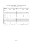 Table B-3
2007 Population-Weighted Sum of Annual Mean PM;5 Predictions Abo've 15.04
RPM Results
Population
Percent Change from 2007 Base Case
0.25
Trading
0.20
Trading
Regionally
1
0.15
Trading
0.12
Trading
SIP Call States
All Populations
Xon- White
Undei 18
(o and o\cr
I,o\\ Income
-46
-45
-46
-4 5
-5 4
-60
-60
-60
-5 9
-87
-68
-65
-68
-68
-11 4
-6~
-63
-68
-6 5
-62
-14 5
-148
-145
-143
-19 1
37 States & B.C.
All Population-.
Non-White
I'ndcr IS
65 and o'\er
Lo\\ Income
-3 0
-3 8
-3 0
-28
-44
-4 1
-5 1
-4 1
-3 9
~~ ~>
-4 5
-5 5
-4 5
-4 4
-93
-46
-5 4
-46
-4 3
-5 2
-100
-128
-99
-95
-159
8 The PM_. annual mear ^landard o! 1 5 g m' (rounded to ihc neaicst 1 ] Oth i a\ craned o\er a ^ \ ear period 1 his anal\Ms i> nol based on an
evien^ne network ol actual P\i_, oh^jnation*- and dtt*.^ nol predict ihree \ears \\orlh ol ajr qualiT\. and i^ therefore not directl\ comparable to the
ofllcia! standard
Page B-3
image:
Table B-3
2007 Population-Weighted Sum of Annual Mean PM;5 Predictions Abo've 15.04
RPM Results
Population
Percent Change from 2007 Base Case
0.25
Trading
0.20
Trading
Regionally
1
0.15
Trading
0.12
Trading
SIP Call States
All Populations
Xon- White
Undei 18
(o and o\cr
I,o\\ Income
-46
-45
-46
-4 5
-5 4
-60
-60
-60
-5 9
-87
-68
-65
-68
-68
-11 4
-6~
-63
-68
-6 5
-62
-14 5
-148
-145
-143
-19 1
37 States & B.C.
All Population-.
Non-White
I'ndcr IS
65 and o'\er
Lo\\ Income
-3 0
-3 8
-3 0
-28
-44
-4 1
-5 1
-4 1
-3 9
~~ ~>
-4 5
-5 5
-4 5
-4 4
-93
-46
-5 4
-46
-4 3
-5 2
-100
-128
-99
-95
-159
8 The PM_. annual mear ^landard o! 1 5 g m' (rounded to ihc neaicst 1 ] Oth i a\ craned o\er a ^ \ ear period 1 his anal\Ms i> nol based on an
evien^ne network ol actual P\i_, oh^jnation*- and dtt*.^ nol predict ihree \ears \\orlh ol ajr qualiT\. and i^ therefore not directl\ comparable to the
ofllcia! standard
Page B-3
image:
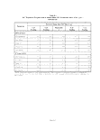 Table B-4
20(17 Population-Weighted Sum of Annual Mean PM,0 Predictions Abo\e 50.-I //g/m3 a:
RPM Resultsb
Population
All Populations
Non-While
Under IS
(o and o\c;
1 ou Income
Percent Change from Base Case
0.25
Trading
-00
-fj 0
-00
-00
-00
0.20
Trading
-00
-00
-oo
-(,0
-0 0
Regionally
1
-00
-o o
-00
-0 0
-00
0.15
Trading
-00
-00
-0 0
-0 0
-0 0
0.12
Trading
-00
-00
-00
-0 0
-00
' Tlu P\l. annual mean Mandard ol 50 . g m' i rounded U> the nearer . g) a\eraged o\er a ^ \ear penod Ihi-. anaK^i-- doe^ not predia thiee \i.
\\onh o! air quahu and is therefore no! dueclK wompa^ahle to the official -.tandard
111 Kvations ha\e predietioiT- helou the PMKi standard hence there are no reduction1- in e\po-;ure<- relatne a 50 ug nr annual mean threshold
Page B-4
image:
Table B-4
20(17 Population-Weighted Sum of Annual Mean PM,0 Predictions Abo\e 50.-I //g/m3 a:
RPM Resultsb
Population
All Populations
Non-While
Under IS
(o and o\c;
1 ou Income
Percent Change from Base Case
0.25
Trading
-00
-fj 0
-00
-00
-00
0.20
Trading
-00
-00
-oo
-(,0
-0 0
Regionally
1
-00
-o o
-00
-0 0
-00
0.15
Trading
-00
-00
-0 0
-0 0
-0 0
0.12
Trading
-00
-00
-00
-0 0
-00
' Tlu P\l. annual mean Mandard ol 50 . g m' i rounded U> the nearer . g) a\eraged o\er a ^ \ear penod Ihi-. anaK^i-- doe^ not predia thiee \i.
\\onh o! air quahu and is therefore no! dueclK wompa^ahle to the official -.tandard
111 Kvations ha\e predietioiT- helou the PMKi standard hence there are no reduction1- in e\po-;ure<- relatne a 50 ug nr annual mean threshold
Page B-4
image:
 Appendix C. EMISSION SUMMARIES FOR BENEFITS-RELATED
AIR QUALITY MODELING
This appendix presents emissions summaries rele\ ant to the air qualm modeling that is used as an
input to the benefits anah ses co\ ered in Chapter 3 The tables in this appendix contain summary emissions
estimates for the entire modeling domain, not just the area co\ered by the SIP call rule Table C-l contains a
summaiA of the ozone season NOx emissions used to drive the regional-scale ozone prediction model. UAM-
V Tables C-2 through C-5 present summaries of the warm and cold season emissions of NOx and SO. used
to drive the secondan PM prediction model. RADM-RPM Tables C-6 and C-7 contain summaries of NOx
and SO- emissions used to dm e the secondan PM prediction model. S-R Matrix Fmalh. for compansion
purposes. Table C-8 presents the emissions associated with the cost anahses for EGU and non-EGU sources
presented in Volume 1 of the RIA Each of these tables presents the emissions for each regulators alternate e
for which benefits estimates are de\eloped
PageC-1
image:
Appendix C. EMISSION SUMMARIES FOR BENEFITS-RELATED
AIR QUALITY MODELING
This appendix presents emissions summaries rele\ ant to the air qualm modeling that is used as an
input to the benefits anah ses co\ ered in Chapter 3 The tables in this appendix contain summary emissions
estimates for the entire modeling domain, not just the area co\ered by the SIP call rule Table C-l contains a
summaiA of the ozone season NOx emissions used to drive the regional-scale ozone prediction model. UAM-
V Tables C-2 through C-5 present summaries of the warm and cold season emissions of NOx and SO. used
to drive the secondan PM prediction model. RADM-RPM Tables C-6 and C-7 contain summaries of NOx
and SO- emissions used to dm e the secondan PM prediction model. S-R Matrix Fmalh. for compansion
purposes. Table C-8 presents the emissions associated with the cost anahses for EGU and non-EGU sources
presented in Volume 1 of the RIA Each of these tables presents the emissions for each regulators alternate e
for which benefits estimates are de\eloped
PageC-1
image:
 Table C-1
O/.onc Season Dailv NO\ Kmissions l>v Major Sector and Regulator) Alternative:
HAM-V Inputs
Major Sector
IX 11 I Poml Sources
Non-IXrU I'oint Sources
2007 Base Case
2.25S 112
MM. 177
0.25 Trading
1 (idd 001
()()S,7I7
0.20 Trading
1.4V) Sh')
X40694
Reg. 1
1.17<S.OXX
1,101,7X4
0. 15 Trading
1,2-=.! VI')
X40.694
O.I 2 Trading
1.1 'IS XOV
X'l(l(i<).|
Table C-2
Warm Season Annuali/cd IMO\ Emissions l»> Major Sector and Regulatory Alternative:
RADM-RPM Inputs
Major Sector
I'XHJ I'oint Sources
Non-l'XHJ I'oint Sources
2007 Base Case
4,')S').()4!
7.9IX.<)4X
0.25 Trading
1.70X,4l>S
6.175.17.1
0.2(t Trading
!.257,42(>
5.424.5X2
Reg. 1
1,075.07')
5.244.24X
0.15 Trading
2,81 1,652
4.XXO.X52
0.12 Trading
2.568,2.15
4,742,169
Table C 3
Warm Season Annuali/,ed SO, Kmissions 1>> Major Sector and Regulators Alternative:
RADM-RPM Inputs
Major Sector
I'XHJ Point Sources
Non-IXHJ Point Sources
2007 Base Case
10,4.57 .8-10
14.100,5X2
0.25 Trading
10. 196, 5X7
14,271.520
0.20 Trading
10.400,771
14.041.149
Reg. 1
10.19x291
14,017.691
0.15 Trading
10,115,766
11,958,1X5
0.12 Trading
i 0,071.X 15
11.715,866
Page C-2
image:
Table C-1
O/.onc Season Dailv NO\ Kmissions l>v Major Sector and Regulator) Alternative:
HAM-V Inputs
Major Sector
IX 11 I Poml Sources
Non-IXrU I'oint Sources
2007 Base Case
2.25S 112
MM. 177
0.25 Trading
1 (idd 001
()()S,7I7
0.20 Trading
1.4V) Sh')
X40694
Reg. 1
1.17<S.OXX
1,101,7X4
0. 15 Trading
1,2-=.! VI')
X40.694
O.I 2 Trading
1.1 'IS XOV
X'l(l(i<).|
Table C-2
Warm Season Annuali/cd IMO\ Emissions l»> Major Sector and Regulatory Alternative:
RADM-RPM Inputs
Major Sector
I'XHJ I'oint Sources
Non-l'XHJ I'oint Sources
2007 Base Case
4,')S').()4!
7.9IX.<)4X
0.25 Trading
1.70X,4l>S
6.175.17.1
0.2(t Trading
!.257,42(>
5.424.5X2
Reg. 1
1,075.07')
5.244.24X
0.15 Trading
2,81 1,652
4.XXO.X52
0.12 Trading
2.568,2.15
4,742,169
Table C 3
Warm Season Annuali/,ed SO, Kmissions 1>> Major Sector and Regulators Alternative:
RADM-RPM Inputs
Major Sector
I'XHJ Point Sources
Non-IXHJ Point Sources
2007 Base Case
10,4.57 .8-10
14.100,5X2
0.25 Trading
10. 196, 5X7
14,271.520
0.20 Trading
10.400,771
14.041.149
Reg. 1
10.19x291
14,017.691
0.15 Trading
10,115,766
11,958,1X5
0.12 Trading
i 0,071.X 15
11.715,866
Page C-2
image:
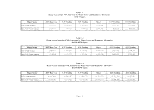 1 able (-4
Cold Season Annuali/,ed NO\ Kmissions by Major Sector and Regulatory Alternative:
RADM-RPM Inputs
Major Sector
1'X'rU Pomt Sources
Non-1 i(HJ Point Sources
2007 Base Case
•J.S60.9M
7/l8l.ln9
0.25 Trading J 0.20 Trading j Reg, 1
•1 IS |.| 47
6,(>00.}25
• 1 151 643
6 300 4X9
LI SO 23(,
6.29X.746
0.15 Trading
4.I4X7SI
6 2V7.002
0.1 2 Trailing |
-I I "') "iX"?
d.2XX.2'.>')
Talilt- C-5
Cold Season Annuali/ed SO, Kmissions In Major Sector and Regulatory Alternative:
RADM-RPM Inputs
Major Sector
I'XHJ Point Sources
Non-1 'X!U Point Sources
2007 Base Case
1>.()XO,7'H
13.623.675
0.25 Trailing
10.100.2X7
nj.n,oss
0.20 Trading
10,1 16,509
M, 759. 3X5
Reg. I
10.156 XX4
n,775.3S3
O.I 5 Trading | O.I 2 Trading
io.nx.9xx
H. 79 1,381
10, 204, 3 IX
I3,X47,!47
image:
1 able (-4
Cold Season Annuali/,ed NO\ Kmissions by Major Sector and Regulatory Alternative:
RADM-RPM Inputs
Major Sector
1'X'rU Pomt Sources
Non-1 i(HJ Point Sources
2007 Base Case
•J.S60.9M
7/l8l.ln9
0.25 Trading J 0.20 Trading j Reg, 1
•1 IS |.| 47
6,(>00.}25
• 1 151 643
6 300 4X9
LI SO 23(,
6.29X.746
0.15 Trading
4.I4X7SI
6 2V7.002
0.1 2 Trailing |
-I I "') "iX"?
d.2XX.2'.>')
Talilt- C-5
Cold Season Annuali/ed SO, Kmissions In Major Sector and Regulatory Alternative:
RADM-RPM Inputs
Major Sector
I'XHJ Point Sources
Non-1 'X!U Point Sources
2007 Base Case
1>.()XO,7'H
13.623.675
0.25 Trailing
10.100.2X7
nj.n,oss
0.20 Trading
10,1 16,509
M, 759. 3X5
Reg. I
10.156 XX4
n,775.3S3
O.I 5 Trading | O.I 2 Trading
io.nx.9xx
H. 79 1,381
10, 204, 3 IX
I3,X47,!47
image:
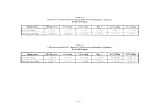 Table C-6
Annual NO\ Emissions h\ Major Sector and Regulators Alternative:
S-R Matrix Inputs
Major Sector
1'Xil ) Point Sources
Non-1 •.(HI Point Sources
2(107 Base Case
4 8(v| Xh')
1,141,0X0
0.25 Trading
1 nx1). 7S(.)
2.172.24X
0.20 Trading
i <)02.UH
2.172 24X
Ri'K- I
l.X2(O(,()
2.372.24S
((.ISTradinj-
\715.75I
2.W2.2.IX
O.I 2 Trading
Tf.l 1,(-7I
2."?72.2'I8
Table ( -7
Annual SO, Emissions b> Major Sector and Regulators Alternative:
S-R Matrix Inputs
Major Sector
1'XiU 1'oint Sources
Non-1 'XilJ Point Sources
2(K>7 Base(ase
10,277.251
\7n.552
0.25 Trading
10.121. 1S^
"?. 711.552
0.20 Trading
10 112,1X4
\711.SS2
Reg. 1
I0.isi.dl5
\7n.552
O.I 5 Trading
I0.10l).')|4
3,711,552
0.12 Trading
10,247.11 1
1,71.1.552
Page C-i
image:
Table C-6
Annual NO\ Emissions h\ Major Sector and Regulators Alternative:
S-R Matrix Inputs
Major Sector
1'Xil ) Point Sources
Non-1 •.(HI Point Sources
2(107 Base Case
4 8(v| Xh')
1,141,0X0
0.25 Trading
1 nx1). 7S(.)
2.172.24X
0.20 Trading
i <)02.UH
2.172 24X
Ri'K- I
l.X2(O(,()
2.372.24S
((.ISTradinj-
\715.75I
2.W2.2.IX
O.I 2 Trading
Tf.l 1,(-7I
2."?72.2'I8
Table ( -7
Annual SO, Emissions b> Major Sector and Regulators Alternative:
S-R Matrix Inputs
Major Sector
1'XiU 1'oint Sources
Non-1 'XilJ Point Sources
2(K>7 Base(ase
10,277.251
\7n.552
0.25 Trading
10.121. 1S^
"?. 711.552
0.20 Trading
10 112,1X4
\711.SS2
Reg. 1
I0.isi.dl5
\7n.552
O.I 5 Trading
I0.10l).')|4
3,711,552
0.12 Trading
10,247.11 1
1,71.1.552
Page C-i
image:
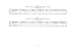 Appendix D. NONLINEAR CHEMISTRY AND FINE PARTICLE PRODUCTION
E\ aluating the effect of major reductions m emissions of nitrogen oxides on particles in made more
difficult because N0\ pla\s an important role in the atmospheric chemistry including formation of nitrate.
organic, and sulfate particles The extent to \\hich Nox reductions reduce fine particle le\els is dependent on
a number of factors that \ an. \vith time and location, including the concentration of ke> reactne gases and
particles, as well as emissions and meteorology The following discussion pro\ ides some background on the
nature of these chemical reactions as a basis for understanding the rele\ ance of non-linear modeling results
D.I Background
The h\ dro\\ 1 radical. OH. is a major oxidi/ing specie in the atmosphere The largest single source of
OH is the breakdown of ozone. O3. b\ ultra\ lolet light in the presence of \\ atcr Clearh. reduction of NOx
can affect the production ofo/one and OH radical in particular locations Sulfate. a major component of fine
particles, is formed b\ the oxidation of SO- through t\vo main path\\a\s gas-phase oxidation and aqueous-
phase oxidation (in \\ater droplets) Sulfate is formed in the gas phase b\ oxidation of SO: b> OH This
process does not use up OH. b\ and large, so a change in SO- produces approximate!} an equnalent change
in S0: Also, an incrcasc'decrease in OH \\ill cause an increase/decrease in gas-phase produced SO4
Sulfate (SO,) is also formed in the aqueous phase in cloud droplets This occurs b\ comersion of
SO- b> h\drogen peroxide. H-0-. and O-, The \ast proportion of the aqueous-phase S0: is produced b\
H-0- for eastern North American conditions This process does use up oxidants If SO- is \ cry high, then
there can be oxidant-hmited conditions, i c . the nonhncarit\ that \\as of concern in NAPAP with respect to
the cffectn eness of acid rain controls Under oxidant-hmited conditions, the production of SO, \\ill be
mosth determined b\ the a\ ailabihn of the oxidant. not b> the a\ ailabihty of SO- Modeling anah sis with
RADM estimates that a majority of the eastern L S sulfate comes from the aqueous-phase oxidation of
sulfur dioxide, the second path\\a\
Nitric acid. HNO,. the precursor to aerosol nitrate, in formed b> N0; combining with OH The
formation of HNO, is a termination reaction and uses up both OH and NO- This reaction is part of the
photochemical process that accounts for the production of O,
The radicals that arc produced during am one da> all disappear or terminate during that da> in a
matter of tens of minutes Production equals termination in the photochemical process There are t\\o
important path\\a\s of termination that are in constant competition
a) OH combines \\ith NO-, taking out one radical If there is a lot of NOx around, this pathwa\ out
competes and inhibits the a\ailabihh of radicals b\ taking so mam OH's out of the action so
quickly If NOx is scarce, then this pathwa> cannot compete as well and a second termination
path\\a> becomes most important
b) In the second mam termination path\\ay. OH combines \\ith itself, to form H-O;. hydroxy radicals
combine with perox> radicals to form organic peroxides Two radicals are taken out
The relatn e fraction of nitrate that exists in the particle phase (as opposed to vapor phase nitric acid
or ammonium nitrate) depends in turn upon the relatne concentration of acid sulfate species and ammonia
In areas \\ith high acid sulfate concentrations (e g the eastern U S. in the summer), nitrate tends to occur in
the vapor phase and reductions of NOx emissions could not result in a large reductions in fine particle
nitrates Where sulfate le\ els are much then nitrate particle le\ els would be higher
PageD-1
image:
Appendix D. NONLINEAR CHEMISTRY AND FINE PARTICLE PRODUCTION
E\ aluating the effect of major reductions m emissions of nitrogen oxides on particles in made more
difficult because N0\ pla\s an important role in the atmospheric chemistry including formation of nitrate.
organic, and sulfate particles The extent to \\hich Nox reductions reduce fine particle le\els is dependent on
a number of factors that \ an. \vith time and location, including the concentration of ke> reactne gases and
particles, as well as emissions and meteorology The following discussion pro\ ides some background on the
nature of these chemical reactions as a basis for understanding the rele\ ance of non-linear modeling results
D.I Background
The h\ dro\\ 1 radical. OH. is a major oxidi/ing specie in the atmosphere The largest single source of
OH is the breakdown of ozone. O3. b\ ultra\ lolet light in the presence of \\ atcr Clearh. reduction of NOx
can affect the production ofo/one and OH radical in particular locations Sulfate. a major component of fine
particles, is formed b\ the oxidation of SO- through t\vo main path\\a\s gas-phase oxidation and aqueous-
phase oxidation (in \\ater droplets) Sulfate is formed in the gas phase b\ oxidation of SO: b> OH This
process does not use up OH. b\ and large, so a change in SO- produces approximate!} an equnalent change
in S0: Also, an incrcasc'decrease in OH \\ill cause an increase/decrease in gas-phase produced SO4
Sulfate (SO,) is also formed in the aqueous phase in cloud droplets This occurs b\ comersion of
SO- b> h\drogen peroxide. H-0-. and O-, The \ast proportion of the aqueous-phase S0: is produced b\
H-0- for eastern North American conditions This process does use up oxidants If SO- is \ cry high, then
there can be oxidant-hmited conditions, i c . the nonhncarit\ that \\as of concern in NAPAP with respect to
the cffectn eness of acid rain controls Under oxidant-hmited conditions, the production of SO, \\ill be
mosth determined b\ the a\ ailabihn of the oxidant. not b> the a\ ailabihty of SO- Modeling anah sis with
RADM estimates that a majority of the eastern L S sulfate comes from the aqueous-phase oxidation of
sulfur dioxide, the second path\\a\
Nitric acid. HNO,. the precursor to aerosol nitrate, in formed b> N0; combining with OH The
formation of HNO, is a termination reaction and uses up both OH and NO- This reaction is part of the
photochemical process that accounts for the production of O,
The radicals that arc produced during am one da> all disappear or terminate during that da> in a
matter of tens of minutes Production equals termination in the photochemical process There are t\\o
important path\\a\s of termination that are in constant competition
a) OH combines \\ith NO-, taking out one radical If there is a lot of NOx around, this pathwa\ out
competes and inhibits the a\ailabihh of radicals b\ taking so mam OH's out of the action so
quickly If NOx is scarce, then this pathwa> cannot compete as well and a second termination
path\\a> becomes most important
b) In the second mam termination path\\ay. OH combines \\ith itself, to form H-O;. hydroxy radicals
combine with perox> radicals to form organic peroxides Two radicals are taken out
The relatn e fraction of nitrate that exists in the particle phase (as opposed to vapor phase nitric acid
or ammonium nitrate) depends in turn upon the relatne concentration of acid sulfate species and ammonia
In areas \\ith high acid sulfate concentrations (e g the eastern U S. in the summer), nitrate tends to occur in
the vapor phase and reductions of NOx emissions could not result in a large reductions in fine particle
nitrates Where sulfate le\ els are much then nitrate particle le\ els would be higher
PageD-1
image:
 D.2 \\ hat this means for NOx Emissions and Sulfate
In urban areas with rclatnch high NOx emissions radical formation and propagation is inhibited If
NOx emissions are reduced b\ small to moderate amounts. O3 and OH \\ill increase Note, the response for
a\ erage 0-. can be different than the response for peak O, If S0: is a^ ailable. then \\here the OH increases.
an increase in the amount of S0; \\ill be oxidized to S0.; in the gas phase This produces a "nonlinear"
response in S>Q. (increase) to a reduction in NOx
In rural areas \\ith relatneh models NOx le\els. O3 and OH \vill decrease \\hen NOx is reduced
Percentagewise, the decrease m O, and OH v>ill less than NOx and NO- The ratio of OH to T\O: \\ill
therefore increase and more of the OH budget \\ill terminate as H:O; This ma\ or ma\ not lead to an
increase in H-O- In the RADM simulations there \\as an increase in H:O; in certain areas, especially o\er
Ohio and western Pcnns\Kama If there is excess S0:. then \\here H:O- increases, in increased amount of
S0: \\ill be comerted to SO, in the aqueous phase This produces a ••nonlinear" response in SO4 The larger
and more pen asn c source of the nonhneanU in these model results seems to be the change in H-0;
The projected relatue abundance of sulfatc \s nitrate particles m future > ears depends upon
assumptions about the cffectneness of acid rain and as \et undecided strategies to implement regional haze
and fine particle standards Under the scenarios examined for this RIA. the sulfate le\ els \\ere high enough to
limit the amount of nitrate aerosol reduction that \\ould accompam a regional NOx reduction If. ho\\e\ er.
future strategies further reduced SOx emissions, the expected reductions in fine particles from NOx
reductions \\ould be decided!) larger, and more linear Because of the uncertainties in the atmospheric
chemistn for these future \ears. the RIA relies on modeling tools that estimate both linear and non-linear
responses for PM reductions
D.3 Reference
Dennis. R L Memorandum to Scott Mathias and John Bachmann. U S EPA Office of Air Quality Planning
and Standards from Robin Dennis. U S EPA. Office of Research and De\elopment. September 17. 1998
Page D-2
image:
D.2 \\ hat this means for NOx Emissions and Sulfate
In urban areas with rclatnch high NOx emissions radical formation and propagation is inhibited If
NOx emissions are reduced b\ small to moderate amounts. O3 and OH \\ill increase Note, the response for
a\ erage 0-. can be different than the response for peak O, If S0: is a^ ailable. then \\here the OH increases.
an increase in the amount of S0; \\ill be oxidized to S0.; in the gas phase This produces a "nonlinear"
response in S>Q. (increase) to a reduction in NOx
In rural areas \\ith relatneh models NOx le\els. O3 and OH \vill decrease \\hen NOx is reduced
Percentagewise, the decrease m O, and OH v>ill less than NOx and NO- The ratio of OH to T\O: \\ill
therefore increase and more of the OH budget \\ill terminate as H:O; This ma\ or ma\ not lead to an
increase in H-O- In the RADM simulations there \\as an increase in H:O; in certain areas, especially o\er
Ohio and western Pcnns\Kama If there is excess S0:. then \\here H:O- increases, in increased amount of
S0: \\ill be comerted to SO, in the aqueous phase This produces a ••nonlinear" response in SO4 The larger
and more pen asn c source of the nonhneanU in these model results seems to be the change in H-0;
The projected relatue abundance of sulfatc \s nitrate particles m future > ears depends upon
assumptions about the cffectneness of acid rain and as \et undecided strategies to implement regional haze
and fine particle standards Under the scenarios examined for this RIA. the sulfate le\ els \\ere high enough to
limit the amount of nitrate aerosol reduction that \\ould accompam a regional NOx reduction If. ho\\e\ er.
future strategies further reduced SOx emissions, the expected reductions in fine particles from NOx
reductions \\ould be decided!) larger, and more linear Because of the uncertainties in the atmospheric
chemistn for these future \ears. the RIA relies on modeling tools that estimate both linear and non-linear
responses for PM reductions
D.3 Reference
Dennis. R L Memorandum to Scott Mathias and John Bachmann. U S EPA Office of Air Quality Planning
and Standards from Robin Dennis. U S EPA. Office of Research and De\elopment. September 17. 1998
Page D-2
image:
 TECHNICAL REPORT DATA
(Please read Ins{mi.tic»is on reverse before completing)
1 REPORT NO
ITA-452/R-98-003ft
3 RECIPIENT'S ACCESSION NO
4 TITLE AND SI BTJTLE
Regulatory Impact Analysis for the NOx SIP Call. FIP. and
Section 126 Petitions
Volume 1: Costs and Economic Impacts
Volume 2: Health and Welfare Benefits
5 REPORT DATE
Volume 1: September 1998
Volume 2: December 1998
6 PERFORMING ORGANIZATION CODE
OAQPS/AQSSD
7 AUTHORiS)
Office of Air Quality Planning and Standards
Office of Atmospheric Programs
8 PERFORMING ORGANIZATION REPORT NO
PERFORMING ORGANIZATION NAME AND ADDRESS
U.S. Environmental Protection Agency
Office of Air Quality Planning and Standards &
Office of Atmospheric Programs
Research Triangle Park. NC 27711
10 PROGRAM ELEMENT NO
11 CONTRACT GRANT NO
i: SPONSORING AGENCY NAME AND ADDRESS
Director
Office of Air Quality Planning and Standards
Office of Air and Radiation
U.S. Environmental Protection Agenc\
Research Triansle Park. NC 27711
13 TYPE OF REPORT AND PERIOD COVERED
M SPONSORING AGENC1 CODE
EPA/200/04
1? SUPPLEMENTARY NOTES
If ABSTRACT
This report contains EPA's estimates of the annual costs and benefits of the final NOx SIP call and the
proposed NOx FIP and CAA section 126 petition actions. The report also contains a brief profile of
potentially affected sources and potential economic impacts.
17 KE^ WORDS AND DOCUMENT ANALYSIS
a DESCRIPTORS
Regulator}7 impact analysis: benefits-cost
comparison
18 DISTRIBUTION STATEMENT
Release Unlimited
b IDENTIFIERS OPEN ENDED TERMS
Air Pollution control
19 SECURITY CLASS (Report)
Unclassified
20 SECURITY CLASS (Page)
Unclassified
c COSATI Field Group
21 NO OF PAGES
22 PRICE
EPA Form 2220-1 (Re\. 4-77) PREVIOUS EDITION IS OBSOLETE
image:
TECHNICAL REPORT DATA
(Please read Ins{mi.tic»is on reverse before completing)
1 REPORT NO
ITA-452/R-98-003ft
3 RECIPIENT'S ACCESSION NO
4 TITLE AND SI BTJTLE
Regulatory Impact Analysis for the NOx SIP Call. FIP. and
Section 126 Petitions
Volume 1: Costs and Economic Impacts
Volume 2: Health and Welfare Benefits
5 REPORT DATE
Volume 1: September 1998
Volume 2: December 1998
6 PERFORMING ORGANIZATION CODE
OAQPS/AQSSD
7 AUTHORiS)
Office of Air Quality Planning and Standards
Office of Atmospheric Programs
8 PERFORMING ORGANIZATION REPORT NO
PERFORMING ORGANIZATION NAME AND ADDRESS
U.S. Environmental Protection Agency
Office of Air Quality Planning and Standards &
Office of Atmospheric Programs
Research Triangle Park. NC 27711
10 PROGRAM ELEMENT NO
11 CONTRACT GRANT NO
i: SPONSORING AGENCY NAME AND ADDRESS
Director
Office of Air Quality Planning and Standards
Office of Air and Radiation
U.S. Environmental Protection Agenc\
Research Triansle Park. NC 27711
13 TYPE OF REPORT AND PERIOD COVERED
M SPONSORING AGENC1 CODE
EPA/200/04
1? SUPPLEMENTARY NOTES
If ABSTRACT
This report contains EPA's estimates of the annual costs and benefits of the final NOx SIP call and the
proposed NOx FIP and CAA section 126 petition actions. The report also contains a brief profile of
potentially affected sources and potential economic impacts.
17 KE^ WORDS AND DOCUMENT ANALYSIS
a DESCRIPTORS
Regulator}7 impact analysis: benefits-cost
comparison
18 DISTRIBUTION STATEMENT
Release Unlimited
b IDENTIFIERS OPEN ENDED TERMS
Air Pollution control
19 SECURITY CLASS (Report)
Unclassified
20 SECURITY CLASS (Page)
Unclassified
c COSATI Field Group
21 NO OF PAGES
22 PRICE
EPA Form 2220-1 (Re\. 4-77) PREVIOUS EDITION IS OBSOLETE
image: