Table Page
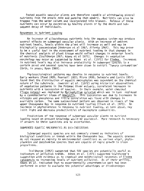
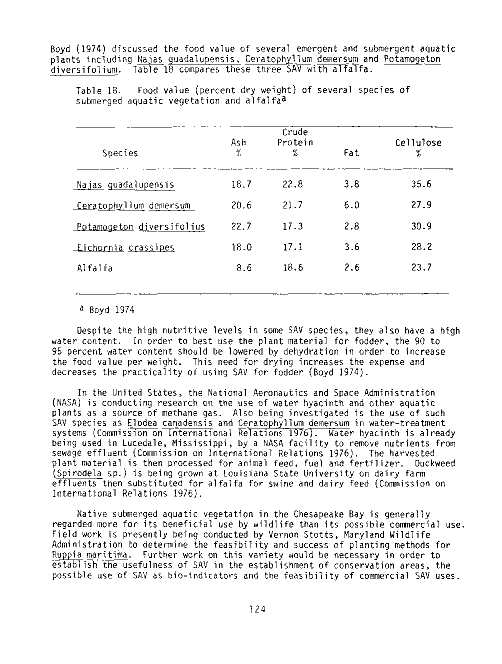
18 Food value (Percent dry weight) of several species of sub-
merged aquatic vegetation and alfalfa 124
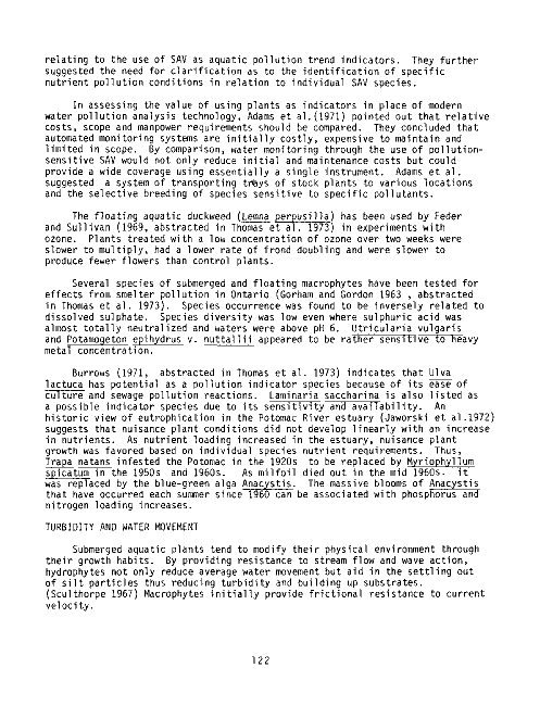
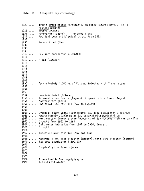
19 Chesapeake Bay chronology 127
20 Occurrence of dominant rooted submerged aquatic vegetation,
Susquehanna Flats Survey, 1958-1975 . 131
21 Frequency of occurrence of submerged aquatic species, Benthic
Survey, 1958-1961 134
22 Frequency of occurrence of vegetated samples, Vegetation
Survey, 1967-1969 136
23 Comparison of relative abundance of rooted submerged plants
in the upper Eastern Bay, Chesapeake Bay, Vegetation Survey,
June-September 1969 137
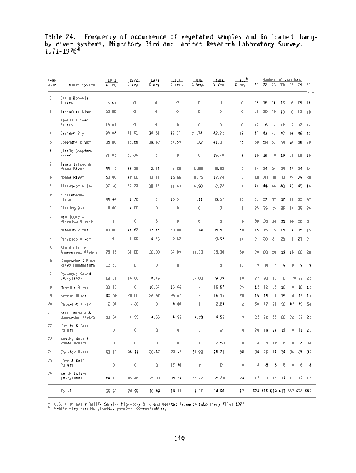
24 Frequency of occurrence of vegetated samples and indicated
change by river system, Migratory Bird and Habitat Research
Laboratory Survey, 1971-1976 .... 140
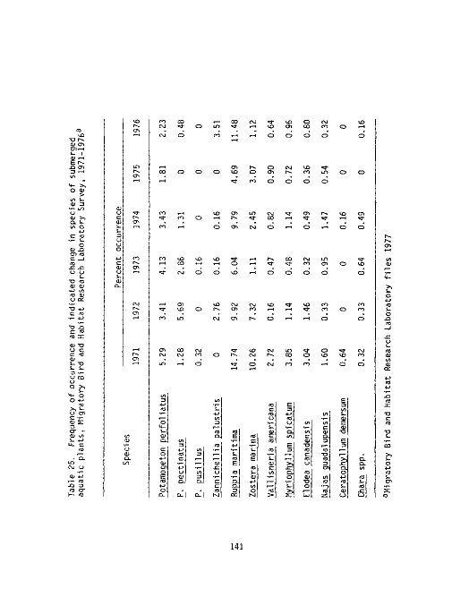
25 Frequency of occurrence and indicated change in species of
submerged aquatic plants, Migratory Bird and Habitat Research
Laboratory Survey, 1971-1976 .... 141
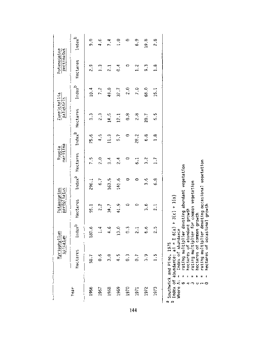
26 Annual abundance of submerged aquatic vegetation in Rhode
River, 1966-1973 143
27 Estimated total coverage of submerged aquatics for major
Virginia sections of the Chesapeake Bay, 1971 and 1974 . . 146
28 Historic documentation key 157
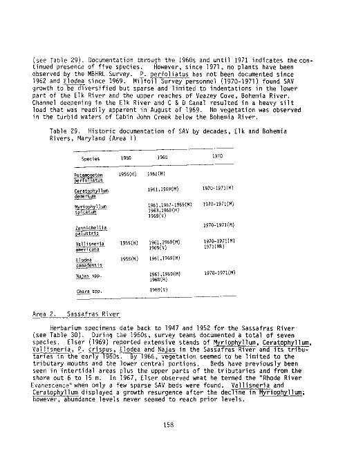
29 . Historic documentation of SAV by decades, Elk and Bohemia
Rivers, Maryland (Area 1) 158
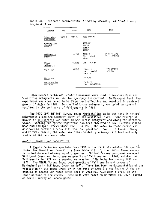
30 Historic documentation of SAV by decades, Sassafras River,
Maryland (Area 2) 159
31 Historic documentation of SAV by decades, Howell and Swan
Points, Maryland (Area 3) 160
32 Historic documentation of SAV by decades, Eastern Bay, Mary-
land (Area 4) 161
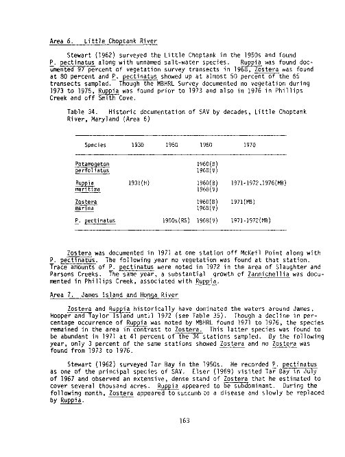
33 Historic documentation of SAV by decades, Choptank River,
Maryland (Area 5) 162
xiv
image:
 Table
34
Historic
documentation
River, Maryland (Area
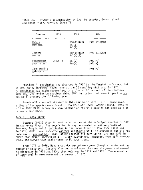
35
Historic
documentation
Honga River, Maryland
36
Historic
documentation
of
6) ,
of
SAV
SAV
by
by
decades ,
decades ,
Little Choptank
James Island and
(Area 7)
of
SAV
by
decades ,
Honga River, Mary-
land (Area 8)
37
38
39
Historic
Mary! and
Historic
Maryland
Historic
documentation
(Area 9) . .
documentation
(Area 10) , ,
documentation
of
of
of
SAV
SAV
SAV
by
by
by
decades ,
decades ,
decades ,
Bloodsworth Island
Susquehanna Flats,
Fishing Bay, Mary-
land (Area 11)
40
41
42
43
Historic
Wi comi co
Historic
Maryland
Historic
Maryl and
Historic
documentation
of
Rivers, Maryland
documentation
(Area 13)
documentation
(Area 14)
documentation
of
of
of
SAV
by
(Area
SAV
SAV
SAV
by
by
by
decades ,
12)
decades ,
decades ,
decades ,
Annemessex Rivers, Maryland (Area 15) . ,
44
Historic
documentation
Bush Rivers, Maryland
45
46
47
48
49
Historic
Maryl and
Historic
Maryland
Historic
Maryland
Historic
Maryl and
Historic
Gunpowder
documentation
(Area 17) ,
documentation
(Area 18) , ,
documentation
,(Area 19) . .
documentation
(Area 20) ,
documentation
" Rivers, Mary
of
SAV
by
decades ,
Nanticoke and
Manokin River,
Patapsco River,
Big and Little
Gunpowder and
(Area 16)
of
of
of
of
of
SAV
SAV
SAV
SAV
SAV
by
by
by
by
by
land (Area
decades ,
decades ,
decades ,
decades ,
decades ,
21) . . ,
Pocomoke Sound,
Magothy River,
Severn River,
Patuxent River,
Back, Middle and
Page
163
164
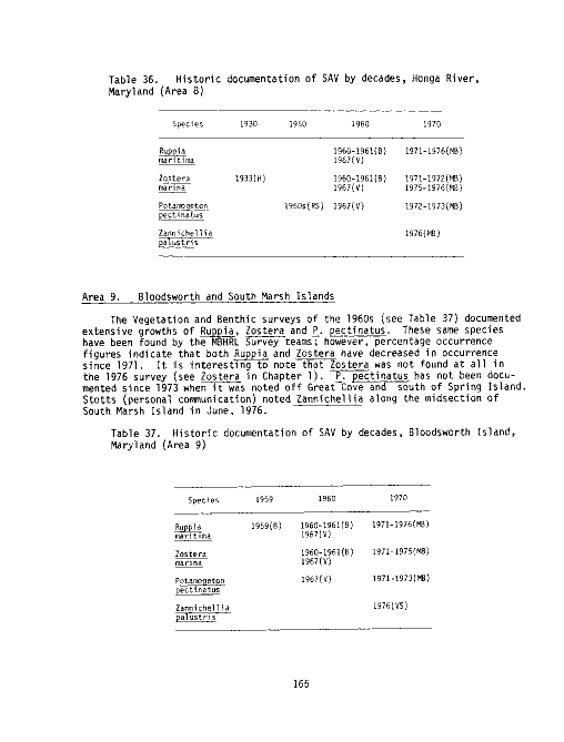
165
165
166
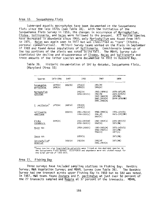
169
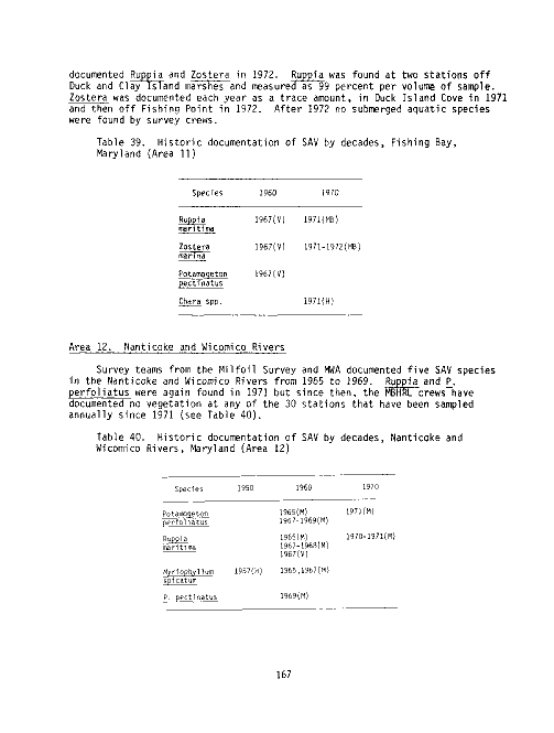
167
168
169
169
170
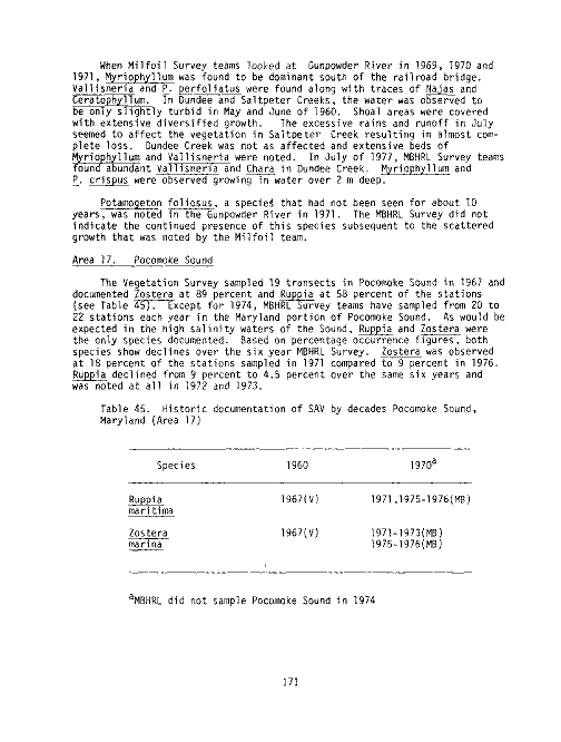
171
172
173
174
175
XV
image:
Table
34
Historic
documentation
River, Maryland (Area
35
Historic
documentation
Honga River, Maryland
36
Historic
documentation
of
6) ,
of
SAV
SAV
by
by
decades ,
decades ,
Little Choptank
James Island and
(Area 7)
of
SAV
by
decades ,
Honga River, Mary-
land (Area 8)
37
38
39
Historic
Mary! and
Historic
Maryland
Historic
documentation
(Area 9) . .
documentation
(Area 10) , ,
documentation
of
of
of
SAV
SAV
SAV
by
by
by
decades ,
decades ,
decades ,
Bloodsworth Island
Susquehanna Flats,
Fishing Bay, Mary-
land (Area 11)
40
41
42
43
Historic
Wi comi co
Historic
Maryland
Historic
Maryl and
Historic
documentation
of
Rivers, Maryland
documentation
(Area 13)
documentation
(Area 14)
documentation
of
of
of
SAV
by
(Area
SAV
SAV
SAV
by
by
by
decades ,
12)
decades ,
decades ,
decades ,
Annemessex Rivers, Maryland (Area 15) . ,
44
Historic
documentation
Bush Rivers, Maryland
45
46
47
48
49
Historic
Maryl and
Historic
Maryland
Historic
Maryland
Historic
Maryl and
Historic
Gunpowder
documentation
(Area 17) ,
documentation
(Area 18) , ,
documentation
,(Area 19) . .
documentation
(Area 20) ,
documentation
" Rivers, Mary
of
SAV
by
decades ,
Nanticoke and
Manokin River,
Patapsco River,
Big and Little
Gunpowder and
(Area 16)
of
of
of
of
of
SAV
SAV
SAV
SAV
SAV
by
by
by
by
by
land (Area
decades ,
decades ,
decades ,
decades ,
decades ,
21) . . ,
Pocomoke Sound,
Magothy River,
Severn River,
Patuxent River,
Back, Middle and
Page
163
164
165
165
166
169
167
168
169
169
170
171
172
173
174
175
XV
image:
 Table Page
50 Historic documentation of SAV by decades, Curtis and Cove
Points, Maryland (Area 22) 176
51 Historic documentation of SAV by decades, South, West and
Rhode Rivers, Maryland (Area 23) 177
52 Historic documentation of SAV by decades, Chester River,
Maryland (Area 24) 178
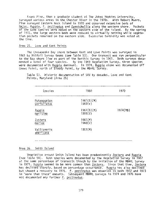
53 Historic documentation of SAV by decades, Love and Kent
Points, Maryland (Area 25) 179
54 Historic documentation of SAV by decades, Smith Island,
Maryland (Area 26) 180
55 Historic documentation of SAV by decades, Upper Potomac
River, Maryland and Virginia (Area 29) 180
56 Historic documentation of SAV by decades, Upper Middle
Potomac River, Maryland and Virginia (Area 30) 181
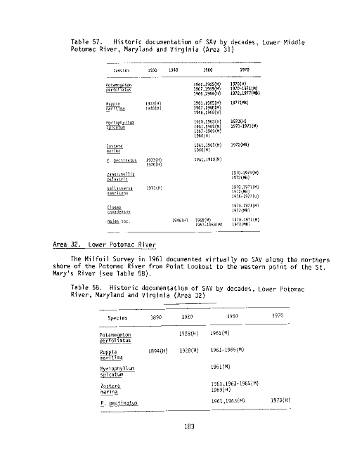
57 Historic documentation of SAV by decades, Lower Middle
Potomac River, Maryland and Virginia, (Area 31) 183
58 Historic documentation of SAV by decades, Lower Potomac
River, Maryland and Virginia (Area 32) 183
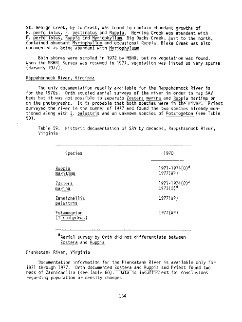
59 Historic documentation of SAV by decades, Rappahannock
River, Virginia 184
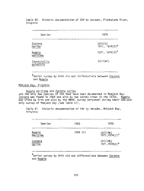
60 Historic documentation of SAV by decades, Piankatank
River, Virginia 185
61 Historic documentation of SAV by decades, Mobjack Bay,
Virginia 185
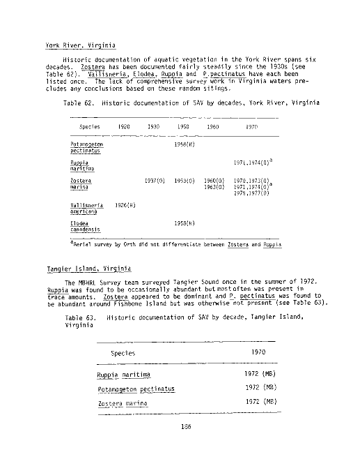
62 Historic documentation of SAV by decades, York River,
Virginia 186
63 Historic documentation of SAV by decades, Tangier Island,
Virginia 186
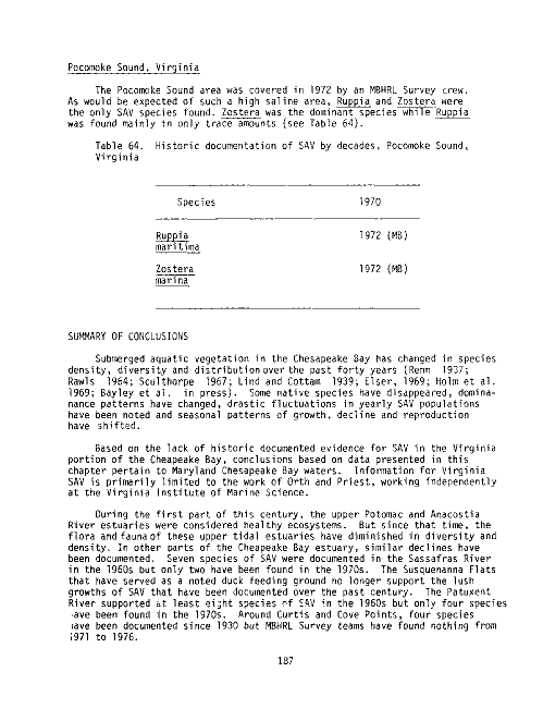
64 Historic documentation of SAV by decades, Pocomoke Sound,
Virginia 187
65 Total farmland in Maryland and Virginia, 1850-1974 .... 190
66 Total fertilizer and lime used in Maryland, 1935-1976 , . , 192
image:
Table Page
50 Historic documentation of SAV by decades, Curtis and Cove
Points, Maryland (Area 22) 176
51 Historic documentation of SAV by decades, South, West and
Rhode Rivers, Maryland (Area 23) 177
52 Historic documentation of SAV by decades, Chester River,
Maryland (Area 24) 178
53 Historic documentation of SAV by decades, Love and Kent
Points, Maryland (Area 25) 179
54 Historic documentation of SAV by decades, Smith Island,
Maryland (Area 26) 180
55 Historic documentation of SAV by decades, Upper Potomac
River, Maryland and Virginia (Area 29) 180
56 Historic documentation of SAV by decades, Upper Middle
Potomac River, Maryland and Virginia (Area 30) 181
57 Historic documentation of SAV by decades, Lower Middle
Potomac River, Maryland and Virginia, (Area 31) 183
58 Historic documentation of SAV by decades, Lower Potomac
River, Maryland and Virginia (Area 32) 183
59 Historic documentation of SAV by decades, Rappahannock
River, Virginia 184
60 Historic documentation of SAV by decades, Piankatank
River, Virginia 185
61 Historic documentation of SAV by decades, Mobjack Bay,
Virginia 185
62 Historic documentation of SAV by decades, York River,
Virginia 186
63 Historic documentation of SAV by decades, Tangier Island,
Virginia 186
64 Historic documentation of SAV by decades, Pocomoke Sound,
Virginia 187
65 Total farmland in Maryland and Virginia, 1850-1974 .... 190
66 Total fertilizer and lime used in Maryland, 1935-1976 , . , 192
image:
 Table Page
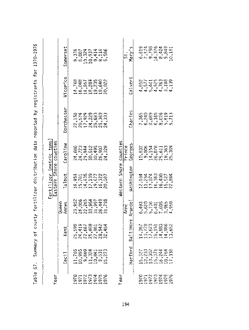
67 Summary of county fertilizer distribution data reported
by registrants for 1970-1976 194
68 Properties of commonly used herbicides 196
69 Atrazine and DCBN applications to four Coastal Plain soil
types 204
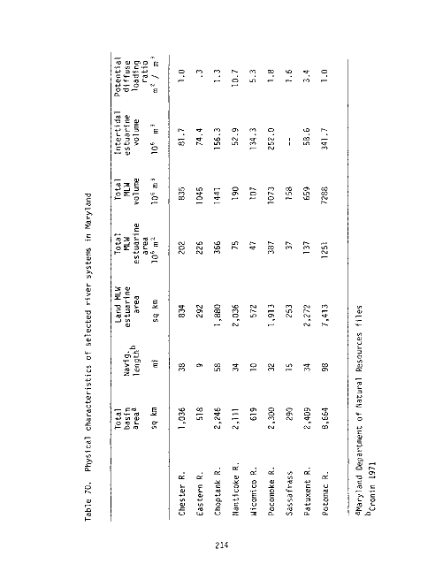
70 Physical characteristics of selected river systems in Mary-
land 214
71 Comparison of land use patterns in upper and lower Choptank
River watershed areas 215
72 Estimates of total amount of specific herbicides used for
weed control in the Choptank River drainage basin, 1975 . 217
73 Potential herbicide leakage, Choptank River drainage basin 218
74 Summary of bioassay results of various concentrations of
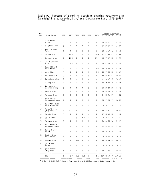
atrazine and linuron on Zannichellia palustris 218
75 Estimate of the use of selected herbicides (kg a.i.) by
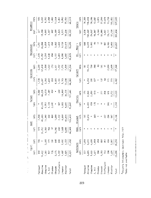
county in Maryland, 1971 and 1975 223
76 Estimate of the use of selected herbicides (kg a.i.) by
county in Virginia, 1971 and 1975 224
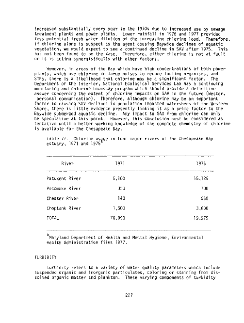
77 Chlorine usage in four major rivers of the Chesapeake Bay
estuary, 1971 and 1975 227
78 Yearly averages of suspended solids (mg/1), Maryland
Chesapeake Bay, 1971-1976 229
79 Average Secchi disk data (cm) by river system, Maryland
Chesapeake Bay, 1972-1976 232
80 Percent of total possible sunlight reaching the surface,
Baltimore-Washington International Airport 233
81 Average salinity (ppt) by river system, Maryland Chesap-
peake Bay, 1971-1976 236
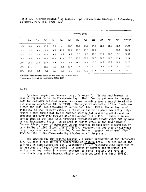
82 Average monthly salinities (ppt), Chesapeake Biological
Laboratory, Solomons, Maryland, 1970-1976 237
83 Naturally occurring soluble concentrations of various heavy
metals in seawater and United States rivers 250
xvn
image:
Table Page
67 Summary of county fertilizer distribution data reported
by registrants for 1970-1976 194
68 Properties of commonly used herbicides 196
69 Atrazine and DCBN applications to four Coastal Plain soil
types 204
70 Physical characteristics of selected river systems in Mary-
land 214
71 Comparison of land use patterns in upper and lower Choptank
River watershed areas 215
72 Estimates of total amount of specific herbicides used for
weed control in the Choptank River drainage basin, 1975 . 217
73 Potential herbicide leakage, Choptank River drainage basin 218
74 Summary of bioassay results of various concentrations of
atrazine and linuron on Zannichellia palustris 218
75 Estimate of the use of selected herbicides (kg a.i.) by
county in Maryland, 1971 and 1975 223
76 Estimate of the use of selected herbicides (kg a.i.) by
county in Virginia, 1971 and 1975 224
77 Chlorine usage in four major rivers of the Chesapeake Bay
estuary, 1971 and 1975 227
78 Yearly averages of suspended solids (mg/1), Maryland
Chesapeake Bay, 1971-1976 229
79 Average Secchi disk data (cm) by river system, Maryland
Chesapeake Bay, 1972-1976 232
80 Percent of total possible sunlight reaching the surface,
Baltimore-Washington International Airport 233
81 Average salinity (ppt) by river system, Maryland Chesap-
peake Bay, 1971-1976 236
82 Average monthly salinities (ppt), Chesapeake Biological
Laboratory, Solomons, Maryland, 1970-1976 237
83 Naturally occurring soluble concentrations of various heavy
metals in seawater and United States rivers 250
xvn
image:
 Table
84
85
86
87
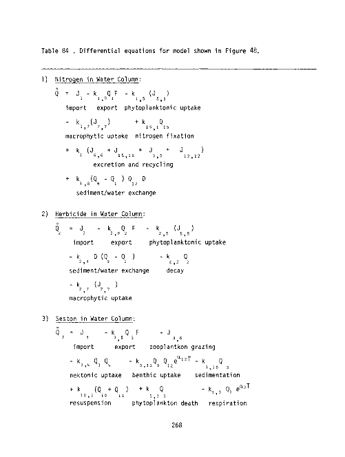
Differential equations for model shown in Figure 48 ....
Special functions used in equations given in Table 84 ...
Differential equations for model shown in Figure 49 ....
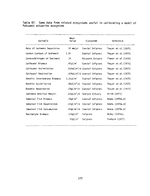
Some data from related ecosystems useful in calibrating a
model of Patuxent estuarine ecosystem
Page
268
273
274
277
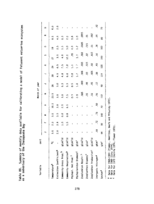
88 Summary of monthly data available for calibrating a model of
Patuxent estuarine ecosystem as a sub-estuary of the Chesa-
peake Bay 278
xvm
image:
Table
84
85
86
87
Differential equations for model shown in Figure 48 ....
Special functions used in equations given in Table 84 ...
Differential equations for model shown in Figure 49 ....
Some data from related ecosystems useful in calibrating a
model of Patuxent estuarine ecosystem
Page
268
273
274
277
88 Summary of monthly data available for calibrating a model of
Patuxent estuarine ecosystem as a sub-estuary of the Chesa-
peake Bay 278
xvm
image:
 LIST OF ABBREVIATIONS AND SYMBOLS
ABBREVIATIONS
o
A
a.e.
a.i.
C
CBCES
CBL
cm
d
dm
9
g cal
ha
HPEL
hr
kg
km
kph
1
m
m2
m3
mm
ml
MHW
MLW
MBHRL
MW
MWA
my
nm
NOAA
PCB
ppb
ppm
PPt
r, r2
SAV
sec
SES
SS
STP
US DA
USDI
USSR
UV
VIMS
angstrom
acid equivalent
active ingredients
celsius
Chesapeake Bay Center for Environmental Studies
Chesapeake Biological Laboratory
centimeter
day
decimeter
gram
gram calorie
hectare
Horn Point Environmental Laboratory
hour
kilogram
kilometer
kilometer per hour
liter
meter
square meter
cubic meter
millimeter
milliliter
mean high water
mean low water
Migratory Bird and Habitat Research Laboratory
megawatt
Maryland Wildlife Administration
millimicron
nanometer
National Oceanic and Atmospheric Administration
polychlorinated biphenyl
parts per billion
parts per million
parts per thousand
correlation coefficient
submerged aquatic vegetation
second
steam electric station
suspended solids
sewage treatment plant
U.S. Department of Agriculture
U.S. Department of Interior
Union of Soviet Socialists Republic
ultra violet
Virginia Institute of Marine Science
microgram
micro Einstein
xix
image:
LIST OF ABBREVIATIONS AND SYMBOLS
ABBREVIATIONS
o
A
a.e.
a.i.
C
CBCES
CBL
cm
d
dm
9
g cal
ha
HPEL
hr
kg
km
kph
1
m
m2
m3
mm
ml
MHW
MLW
MBHRL
MW
MWA
my
nm
NOAA
PCB
ppb
ppm
PPt
r, r2
SAV
sec
SES
SS
STP
US DA
USDI
USSR
UV
VIMS
angstrom
acid equivalent
active ingredients
celsius
Chesapeake Bay Center for Environmental Studies
Chesapeake Biological Laboratory
centimeter
day
decimeter
gram
gram calorie
hectare
Horn Point Environmental Laboratory
hour
kilogram
kilometer
kilometer per hour
liter
meter
square meter
cubic meter
millimeter
milliliter
mean high water
mean low water
Migratory Bird and Habitat Research Laboratory
megawatt
Maryland Wildlife Administration
millimicron
nanometer
National Oceanic and Atmospheric Administration
polychlorinated biphenyl
parts per billion
parts per million
parts per thousand
correlation coefficient
submerged aquatic vegetation
second
steam electric station
suspended solids
sewage treatment plant
U.S. Department of Agriculture
U.S. Department of Interior
Union of Soviet Socialists Republic
ultra violet
Virginia Institute of Marine Science
microgram
micro Einstein
xix
image:
 LIST OF ABBREVIATIONS AND SYMBOLS (cont.)
SYMBOLS
Br, Br"
C, C++
"C
Ca, Ca++
CaCl2
CaCOs
Ca(HC02)?.
Ca(OH}2
C02
14CO?
Cu <-
H
HC1
H2C03
HC03~
H2S
Hg
HgCi2
K
K2C03
KHC03
Mg, Mg
N
NH^, N
NH^-N
Na, Na
Nad
NaAs02
NaHC03
N-P-K
N03, N
N03-N
02
P
TKN
++
bromine, bromine ion
carbon, carbon ion
carbon 14
calcium, calcium ion
calcium chloride
calcium carbonate
calcium formate
calcium hydroxide
carbon dioxide
labeled carbon dioxide
copper
copper sulfate
hydrogen
hydrochloric acid
bicarbonate
bicarbonate ion
hydrogen sulfide
mercury
mercurous chloride
potassium
potassium carbonate
potassium carbonate, acid
magnesium, magnesium ion
nitrogen
ammonia, ammonium ion
ammonia nitrogen
sodium, sodium ion
sodium chloride
sodium arsenite
sodium bicarbonate
nitrogen-phosphorus-potassium
nitrate, nitrate ion
nitrate nitrogen
oxygen
phosphorus
total kjeldahl nitrogen
xx
image:
LIST OF ABBREVIATIONS AND SYMBOLS (cont.)
SYMBOLS
Br, Br"
C, C++
"C
Ca, Ca++
CaCl2
CaCOs
Ca(HC02)?.
Ca(OH}2
C02
14CO?
Cu <-
H
HC1
H2C03
HC03~
H2S
Hg
HgCi2
K
K2C03
KHC03
Mg, Mg
N
NH^, N
NH^-N
Na, Na
Nad
NaAs02
NaHC03
N-P-K
N03, N
N03-N
02
P
TKN
++
bromine, bromine ion
carbon, carbon ion
carbon 14
calcium, calcium ion
calcium chloride
calcium carbonate
calcium formate
calcium hydroxide
carbon dioxide
labeled carbon dioxide
copper
copper sulfate
hydrogen
hydrochloric acid
bicarbonate
bicarbonate ion
hydrogen sulfide
mercury
mercurous chloride
potassium
potassium carbonate
potassium carbonate, acid
magnesium, magnesium ion
nitrogen
ammonia, ammonium ion
ammonia nitrogen
sodium, sodium ion
sodium chloride
sodium arsenite
sodium bicarbonate
nitrogen-phosphorus-potassium
nitrate, nitrate ion
nitrate nitrogen
oxygen
phosphorus
total kjeldahl nitrogen
xx
image:
 ACKNOWLEDGMENTS
Special contributors to this technical document include: Robert Orth,
Virginia Institute of Marine Science, (the biology of Zostera marina) :
Charles K. Rawls, University of Maryland Chesapeake Biological Laboratory,
(the biology of Myriophyll urn spicatum) ; and W. Michael Kemp, University of
Maryland Chesapeake Biological Laboratory (presently at Horn Point Environ-
mental Laboratory) and Fred Lipschultz, University of Maryland Department of
Botany), (the use of models). Further contributors include: Mt.'lon Lewis,
University of Maryland Department of Botany, (the environmental tors
bicarbonate ion and epiphytes); Lorie Stap, University of Marylt ^artment
of Botany, (herbicide survey and waterfowl research); and Waltet . ^iest,
Virginia Institute of Marine Science, (Middlesex County, Virginia, .u.nenta-
tion survey data).
Special thanks are extended to Robin Autenreith and Diane La
University of Maryland Department of Botany, for their research support,
Vernon D. Stotts, Maryland Wildlife Administration, for his constant support
and encouragement; Robert Munro, U.S. Fish and Wildlife Service Migratory
Bird and Habitat Research Laboratory, for the use of data files; and W.S.
Vaugh, W/V Associates, for a preliminary information synthesis on herbicides.
This document is the result of the work of David Flemer (presently with
the U.S. Environmental Protection Agency) who saw the need for a literature
summary and information synthesis. He organized the cooperative funding from
the three agencies involved (U.S. Environmental Protection Agency, U.S. Fish
and Wildlife Service and the Maryland Department of Natural Resources) in
order to initiate this project.
The authors also wish to acknowledge the editorial assistance of Howard
Tait, U.S. Fish and Wildlife Service National Coastal Ecosystems Team; Richard
R. Anderson, The American University; Glenn E. Moore, Commonwealth of Virginia
Water Control Board; David L. Correll, Smithsonian Chesapeake Bay Center for
Environmental Studies; Paul F. Springer, Humbolt State University; George
Fenwick, The Johns Hopkins University; Suzanne Bayley, Maryland Coastal Zone
Management; Gerald Walsh, U.S. Environmental Protection Agency Gulf Breeze
Laboratory; and John Steenis. Glenn Patterson, University of Maryland Depart-
ment of Botany and Stephen Sulkin, University of Maryland Horn Point Environment-
al Laboratory generously provided office space and materials for the production
of this document. Eugene Cronin, Chesapeake Research Consortium; and Frank
Hamons and Kathy Schaeffer, Maryland Department of Natural Resources, provided
continual encouragement and coordination. And without whom this final docu-
ment would not have been possible, we thank Nancy Robbins, Carolyn Hurley and Nancy
Jones, office personnel.
xx i
image:
ACKNOWLEDGMENTS
Special contributors to this technical document include: Robert Orth,
Virginia Institute of Marine Science, (the biology of Zostera marina) :
Charles K. Rawls, University of Maryland Chesapeake Biological Laboratory,
(the biology of Myriophyll urn spicatum) ; and W. Michael Kemp, University of
Maryland Chesapeake Biological Laboratory (presently at Horn Point Environ-
mental Laboratory) and Fred Lipschultz, University of Maryland Department of
Botany), (the use of models). Further contributors include: Mt.'lon Lewis,
University of Maryland Department of Botany, (the environmental tors
bicarbonate ion and epiphytes); Lorie Stap, University of Marylt ^artment
of Botany, (herbicide survey and waterfowl research); and Waltet . ^iest,
Virginia Institute of Marine Science, (Middlesex County, Virginia, .u.nenta-
tion survey data).
Special thanks are extended to Robin Autenreith and Diane La
University of Maryland Department of Botany, for their research support,
Vernon D. Stotts, Maryland Wildlife Administration, for his constant support
and encouragement; Robert Munro, U.S. Fish and Wildlife Service Migratory
Bird and Habitat Research Laboratory, for the use of data files; and W.S.
Vaugh, W/V Associates, for a preliminary information synthesis on herbicides.
This document is the result of the work of David Flemer (presently with
the U.S. Environmental Protection Agency) who saw the need for a literature
summary and information synthesis. He organized the cooperative funding from
the three agencies involved (U.S. Environmental Protection Agency, U.S. Fish
and Wildlife Service and the Maryland Department of Natural Resources) in
order to initiate this project.
The authors also wish to acknowledge the editorial assistance of Howard
Tait, U.S. Fish and Wildlife Service National Coastal Ecosystems Team; Richard
R. Anderson, The American University; Glenn E. Moore, Commonwealth of Virginia
Water Control Board; David L. Correll, Smithsonian Chesapeake Bay Center for
Environmental Studies; Paul F. Springer, Humbolt State University; George
Fenwick, The Johns Hopkins University; Suzanne Bayley, Maryland Coastal Zone
Management; Gerald Walsh, U.S. Environmental Protection Agency Gulf Breeze
Laboratory; and John Steenis. Glenn Patterson, University of Maryland Depart-
ment of Botany and Stephen Sulkin, University of Maryland Horn Point Environment-
al Laboratory generously provided office space and materials for the production
of this document. Eugene Cronin, Chesapeake Research Consortium; and Frank
Hamons and Kathy Schaeffer, Maryland Department of Natural Resources, provided
continual encouragement and coordination. And without whom this final docu-
ment would not have been possible, we thank Nancy Robbins, Carolyn Hurley and Nancy
Jones, office personnel.
xx i
image:
 The Fish and Wildlife Service is grateful to the Chesapeake
Research Consortium for its financial support in printing this
publication, which has enabled a wider dissemination than would have
otherwise been possible.
xxii
image:
The Fish and Wildlife Service is grateful to the Chesapeake
Research Consortium for its financial support in printing this
publication, which has enabled a wider dissemination than would have
otherwise been possible.
xxii
image:
 CHAPTER 1
BIOLOGY
INTRODUCTION
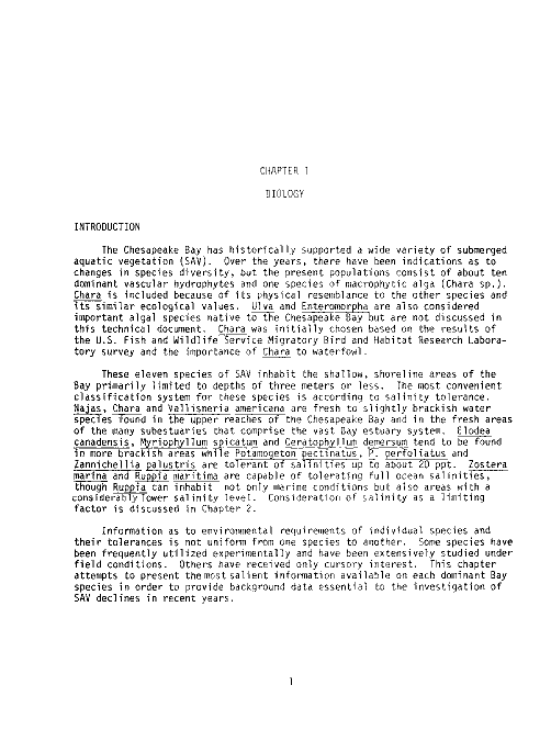
The Chesapeake Bay has historically supported a wide variety of submerged
aquatic vegetation (SAV). Over the years, there have been indications as to
changes in species diversity, but the present populations consist of about ten
dominant vascular hydrophytes and one species of macrophytic alga (Chara sp.).
Chara is included because of its physical resemblance to the other species and
its similar ecological values. Diva and Enteromorpha are also considered
important algal species native to the Chesapeake Bay but are not discussed in
this technical document. Chara was initially chosen based on the results of
the U.S. Fish and Wildlife Service Migratory Bird and Habitat Research Labora-
tory survey and the importance of Chara to waterfowl.
These eleven species of SAV inhabit the shallow, shoreline areas of the
Bay primarily limited to depths of three meters or less. The most convenient
classification system for these species is according to salinity tolerance.
Najas. Chara and Vallisneria americana are fresh to slightly brackish water
species found in the upper reaches of the Chesapeake Bay and in the fresh areas
of the many subestuaries that comprise the vast Bay estuary system. Elodea
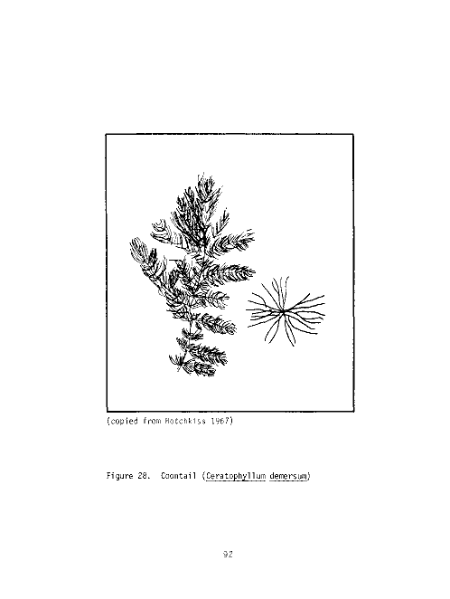
canadensis, Myriophyllum spicatum and Ceratophyllum demersum tend to be found
in more brackish areas while Potamogeton pectinatus, P_. perfoliatus and
Zannichellia palustris are tolerant of salinities up to about 20 ppt. Zostera
marina and Ruppia maritima are capable of tolerating full ocean salinities,
though Ruppia can inhabit not only marine conditions but also areas with a
considerably lower salinity level. Consideration of salinity as a limiting
factor is discussed in Chapter 2.
Information as to environmental requirements of individual species and
their tolerances is not uniform from one species to another. Some species have
been frequently utilized experimentally and have been extensively studied under
field conditions. Others have received only cursory interest. This chapter
attempts to present the most salient information available on each dominant Bay
species in order to provide background data essential to the investigation of
SAV declines in recent years.
image:
CHAPTER 1
BIOLOGY
INTRODUCTION
The Chesapeake Bay has historically supported a wide variety of submerged
aquatic vegetation (SAV). Over the years, there have been indications as to
changes in species diversity, but the present populations consist of about ten
dominant vascular hydrophytes and one species of macrophytic alga (Chara sp.).
Chara is included because of its physical resemblance to the other species and
its similar ecological values. Diva and Enteromorpha are also considered
important algal species native to the Chesapeake Bay but are not discussed in
this technical document. Chara was initially chosen based on the results of
the U.S. Fish and Wildlife Service Migratory Bird and Habitat Research Labora-
tory survey and the importance of Chara to waterfowl.
These eleven species of SAV inhabit the shallow, shoreline areas of the
Bay primarily limited to depths of three meters or less. The most convenient
classification system for these species is according to salinity tolerance.
Najas. Chara and Vallisneria americana are fresh to slightly brackish water
species found in the upper reaches of the Chesapeake Bay and in the fresh areas
of the many subestuaries that comprise the vast Bay estuary system. Elodea
canadensis, Myriophyllum spicatum and Ceratophyllum demersum tend to be found
in more brackish areas while Potamogeton pectinatus, P_. perfoliatus and
Zannichellia palustris are tolerant of salinities up to about 20 ppt. Zostera
marina and Ruppia maritima are capable of tolerating full ocean salinities,
though Ruppia can inhabit not only marine conditions but also areas with a
considerably lower salinity level. Consideration of salinity as a limiting
factor is discussed in Chapter 2.
Information as to environmental requirements of individual species and
their tolerances is not uniform from one species to another. Some species have
been frequently utilized experimentally and have been extensively studied under
field conditions. Others have received only cursory interest. This chapter
attempts to present the most salient information available on each dominant Bay
species in order to provide background data essential to the investigation of
SAV declines in recent years.
image:
 POTAMOGETON PERFOLIATUS
Biology
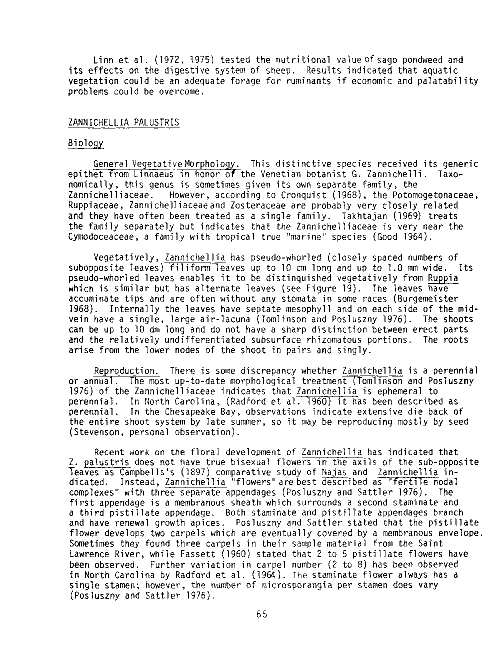
General Vegetative Morphology. Potamogeton perfoliatus exhibits exten-
sive morphological variation and has been separated into two varieties.
Formerly, these two varieties were denoted as separate species, but have since
been denoted as var. bupleuroides and var. richardsonii. Potamogeton
perfoliatus var. bupleuroides will be reviewed in this section since it is the
most common variety found in the Chesapeake Bay (Ogden 1943). For simplicity,
this variety will be referred to as P_. perfoliatus and is commonly known as
redhead grass.
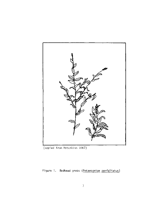
The delicate leaves of this species are flat, scarcely crisped at the
margin and have from 7 to 17 nerves (Ogden 1943) (see Figure 1). The upper
leaves are ovate, 1 to 3 cm long, while the lower leaves are ovate to lanceo-
late, 2.B to 4.5 cm long (Fernald 1970). All of the leaf bases are cordate-
clasping which is a characteristic referred to by this species' name.
Fernald (1970) further characterized the species. Stems are slender and
straight and the lower stem is simple, becoming more branched toward the upper
portion of the plant. Stipules are short and inconspicuous; peduncles are
slender, 2 to 6 cm long; spikes are 0.7 to 2 cm long; and fruit is slender,
obovoid, and 2.5 to 3.2 mm long.
Potamogeton perfoliatus is distinct from other members of the genus due
to its conspicuously heterophyllus foliage yet completely submerged existence
(Schulthope 1967). Variation among this species is so great that two plants
grown from a single rhizome or isolated branched stems can appear to be sep-
arate species (Ogden 1943). Arber (1920)observed a shoot of £. perfoliatus
placed in a rainwater tub and found that when the larger leaves decayed after
a few months, the new leaves were so much narrower and less perfoliate that
it was difficult to relate the two forms of the plant to the same species.
In areas of limited depth, foliage of IP. perfoliatus tends to become less
brilliant green, shorter, broader and thicker (Hutchinson 1975). A represent-
ative series of leaf measurements by Pearsall and Pearsall (1923) indicated
that water depths also influence the ratios of leaf length to leaf breadth.
Their experiments in Lake Windermere indicated that at a 6 m depth, IP.
perfoliatus leaves displayed a 4 to 1 ratio (7.0 cm length to 1.7 cm breadth)
as compared to a 3 m depth where the leaf ratio was 2 to I (3.3 cm length to
1.4 cm breadth).
Factors other than depth operate to alter the morphology of P_. perfoliatus.
Pearsall and Pearsall (1923) believed that a short, broad-leaf form was char-
acteristic of more calcareous substrata (1600 ppm Ca(C03)2 in dry littoral mud).
The extreme lanceolate form occurred on much less calcareous sediment (90 ppm
Ca(Co3)2 in dry littoral mud). Pearsall and Hanby (1925) suggested that calcium
enhanced the permeability of dividing cells and promoted cell division while
potassium promoted cell elongation.
image:
POTAMOGETON PERFOLIATUS
Biology
General Vegetative Morphology. Potamogeton perfoliatus exhibits exten-
sive morphological variation and has been separated into two varieties.
Formerly, these two varieties were denoted as separate species, but have since
been denoted as var. bupleuroides and var. richardsonii. Potamogeton
perfoliatus var. bupleuroides will be reviewed in this section since it is the
most common variety found in the Chesapeake Bay (Ogden 1943). For simplicity,
this variety will be referred to as P_. perfoliatus and is commonly known as
redhead grass.
The delicate leaves of this species are flat, scarcely crisped at the
margin and have from 7 to 17 nerves (Ogden 1943) (see Figure 1). The upper
leaves are ovate, 1 to 3 cm long, while the lower leaves are ovate to lanceo-
late, 2.B to 4.5 cm long (Fernald 1970). All of the leaf bases are cordate-
clasping which is a characteristic referred to by this species' name.
Fernald (1970) further characterized the species. Stems are slender and
straight and the lower stem is simple, becoming more branched toward the upper
portion of the plant. Stipules are short and inconspicuous; peduncles are
slender, 2 to 6 cm long; spikes are 0.7 to 2 cm long; and fruit is slender,
obovoid, and 2.5 to 3.2 mm long.
Potamogeton perfoliatus is distinct from other members of the genus due
to its conspicuously heterophyllus foliage yet completely submerged existence
(Schulthope 1967). Variation among this species is so great that two plants
grown from a single rhizome or isolated branched stems can appear to be sep-
arate species (Ogden 1943). Arber (1920)observed a shoot of £. perfoliatus
placed in a rainwater tub and found that when the larger leaves decayed after
a few months, the new leaves were so much narrower and less perfoliate that
it was difficult to relate the two forms of the plant to the same species.
In areas of limited depth, foliage of IP. perfoliatus tends to become less
brilliant green, shorter, broader and thicker (Hutchinson 1975). A represent-
ative series of leaf measurements by Pearsall and Pearsall (1923) indicated
that water depths also influence the ratios of leaf length to leaf breadth.
Their experiments in Lake Windermere indicated that at a 6 m depth, IP.
perfoliatus leaves displayed a 4 to 1 ratio (7.0 cm length to 1.7 cm breadth)
as compared to a 3 m depth where the leaf ratio was 2 to I (3.3 cm length to
1.4 cm breadth).
Factors other than depth operate to alter the morphology of P_. perfoliatus.
Pearsall and Pearsall (1923) believed that a short, broad-leaf form was char-
acteristic of more calcareous substrata (1600 ppm Ca(C03)2 in dry littoral mud).
The extreme lanceolate form occurred on much less calcareous sediment (90 ppm
Ca(Co3)2 in dry littoral mud). Pearsall and Hanby (1925) suggested that calcium
enhanced the permeability of dividing cells and promoted cell division while
potassium promoted cell elongation.
image:
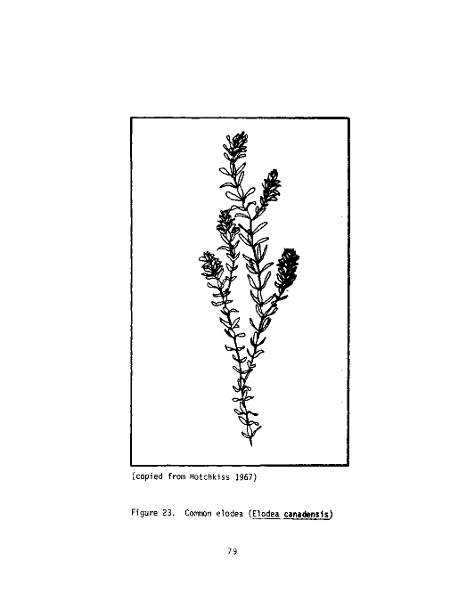
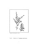
 (copied from Hotchkiss 1967)
Figure 1. Redhead grass (Potampgeton perfoliatus)
image:
(copied from Hotchkiss 1967)
Figure 1. Redhead grass (Potampgeton perfoliatus)
image:
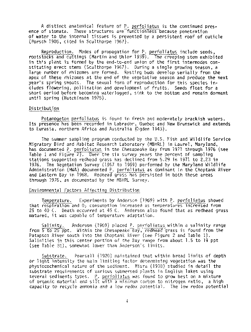
 A distinct anatomical feature of P_. perfoliatus is the continued pres-
ence of stomata. These structures are functionless because penetration
of water to the internal tissues is prevented by a persistent roof of cuticle
(Porsch 1905, cited in Sculthorpe 1967).
Reproduction. Modes of propagation for P_. perfoliatus include seeds,
rootstocks and cuttings (Martin and Uhler 1939). The creeping stem exhibited
in this plant is formed by the end-to-end union of the first internodes con-
stituting erect stems (Sculthorpe 1967). During a single growing season, a
large number of rhizomes are formed. Resting buds develop serially from the
apex of these rhizomes at the end of the vegetative season and produce the next
year's spring shoots. The sexual form of reproduction for this species in-
cludes flowering, pollination and development of fruits. Seeds float for a
short period before becoming waterlogged, sink to the bottom and remain dormant
until spring (Hutchinson 1975).
Distribution
Potamogeton perfoliatus is found in fresh and moderately brackish waters.
Its presence has been recorded in Labrador, Quebec and New Brunswick and extends
to Eurasia, northern Africa and Australia (Ogden 1943).
The summer sampling program conducted by the U.S. Fish and Wildlife Service
Migratory Bird and Habitat Research Laboratory (MBHRL) in Laurel, Maryland,
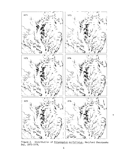
has documented P_. perfoliatus in the Chesapeake Bay from 1971 through 1976 (see
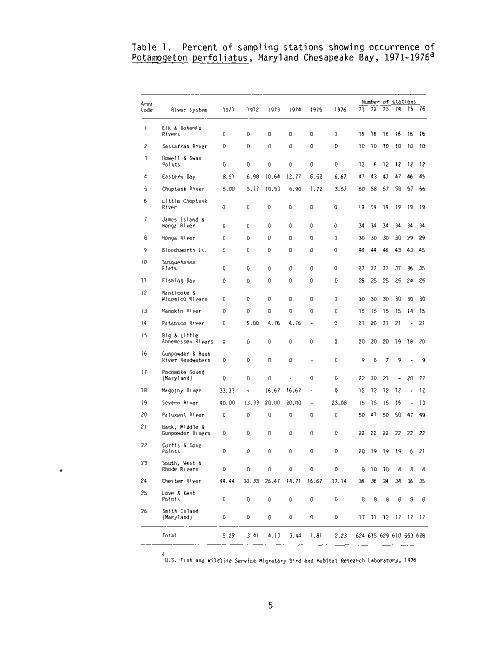
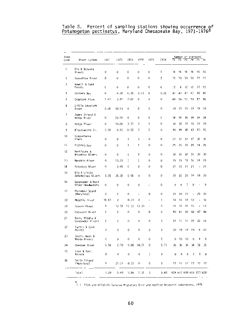
Table 1 and Figure 2).Over the six survey years the percent of sampling
stations supporting redhead grass has declined from 5.29 in 1971 to 2.23 in
1976. The Vegetation Survey (1967 to 1969) performed by the Maryland Wildlife
Administration (MWA) documented P_. perfoliatus as dominant in the Choptank River
and Eastern Bay in 1968. Redhead grass has persisted in both these areas
through 1976, as documented by the MBHRL Survey.
Environmental Factors Affecting Distribution
Temperature. Experiments by Anderson (1969) with P_. perfoliatus showed
that respiration and 02 consumption increased as temperatures increased from
25 to 40 C. Death occurred at 45 C. Anderson also found that as redhead grass
matured, it was capable of temperature adaptation.
Salinity. Anderson (1969) placed P_. perfoliatus within a salinity range
from 5 to 25 ppt. Within the Chesapeake Bay, redhead grass is found from the
Patapsco River south into the Choptank River (see Figure 2 and Table 1).
Salinities in this center portion of the Bay range from about 1.5 to 19 ppt
(see Table 81), somewhat lower than Anderson's limits.
Substrate. Pearsall (1920) maintained that within broad limits of depth
or light intensity the main limiting factor determining vegetation was the
physiocochemical nature of the sediment. Misra (1938) studied in detail the
substrate requirements of various submersed plants in English lakes using
several sediments types. £_. perfoliatus was found to grow best on a mixture
of organic material and silt with a minimum carbon to nitrogen ratio, a high
capacity to recycle ammonia and a low redox potential. The low redox potential
image:
A distinct anatomical feature of P_. perfoliatus is the continued pres-
ence of stomata. These structures are functionless because penetration
of water to the internal tissues is prevented by a persistent roof of cuticle
(Porsch 1905, cited in Sculthorpe 1967).
Reproduction. Modes of propagation for P_. perfoliatus include seeds,
rootstocks and cuttings (Martin and Uhler 1939). The creeping stem exhibited
in this plant is formed by the end-to-end union of the first internodes con-
stituting erect stems (Sculthorpe 1967). During a single growing season, a
large number of rhizomes are formed. Resting buds develop serially from the
apex of these rhizomes at the end of the vegetative season and produce the next
year's spring shoots. The sexual form of reproduction for this species in-
cludes flowering, pollination and development of fruits. Seeds float for a
short period before becoming waterlogged, sink to the bottom and remain dormant
until spring (Hutchinson 1975).
Distribution
Potamogeton perfoliatus is found in fresh and moderately brackish waters.
Its presence has been recorded in Labrador, Quebec and New Brunswick and extends
to Eurasia, northern Africa and Australia (Ogden 1943).
The summer sampling program conducted by the U.S. Fish and Wildlife Service
Migratory Bird and Habitat Research Laboratory (MBHRL) in Laurel, Maryland,
has documented P_. perfoliatus in the Chesapeake Bay from 1971 through 1976 (see
Table 1 and Figure 2).Over the six survey years the percent of sampling
stations supporting redhead grass has declined from 5.29 in 1971 to 2.23 in
1976. The Vegetation Survey (1967 to 1969) performed by the Maryland Wildlife
Administration (MWA) documented P_. perfoliatus as dominant in the Choptank River
and Eastern Bay in 1968. Redhead grass has persisted in both these areas
through 1976, as documented by the MBHRL Survey.
Environmental Factors Affecting Distribution
Temperature. Experiments by Anderson (1969) with P_. perfoliatus showed
that respiration and 02 consumption increased as temperatures increased from
25 to 40 C. Death occurred at 45 C. Anderson also found that as redhead grass
matured, it was capable of temperature adaptation.
Salinity. Anderson (1969) placed P_. perfoliatus within a salinity range
from 5 to 25 ppt. Within the Chesapeake Bay, redhead grass is found from the
Patapsco River south into the Choptank River (see Figure 2 and Table 1).
Salinities in this center portion of the Bay range from about 1.5 to 19 ppt
(see Table 81), somewhat lower than Anderson's limits.
Substrate. Pearsall (1920) maintained that within broad limits of depth
or light intensity the main limiting factor determining vegetation was the
physiocochemical nature of the sediment. Misra (1938) studied in detail the
substrate requirements of various submersed plants in English lakes using
several sediments types. £_. perfoliatus was found to grow best on a mixture
of organic material and silt with a minimum carbon to nitrogen ratio, a high
capacity to recycle ammonia and a low redox potential. The low redox potential
image:
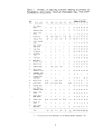
 Table 1. Percent of sampling stations showing occurrence of
Potamogeton perfpliatus, Maryland Chesapeake Bay, 1971-19763
Area
Code
1
2
3
4
5
6
7
8
9
10
11
12
13
14
15
16
17
18
19
20
21
22
23
24
25
26
Number of
River system
Elk & Bohemia
Rivers
Sassafras River
Howell 8 Swan
Points
Eastern Bay
Choptank River
Little Choptank
River
James Island 8
Honga River
Honga River
Bloodsworth Is.
Susquehanna
Flats
Fishing Bay
Nanticoke &
Wicomico Rivers
Manokin River
Patapsco River
Big & Little
Annemessex Rivers
Gunpowder 8 Bush
River Headwaters
Pocomoke Sound
(Maryland)
Magothy River
Severn River
Patuxent River
Back, Middle 8
Gunpowder Rivers
Curtis 8 Cove
Points
South, West &
Rhode Rivers
Chester River
Love 8 Kent
Points
Smith Island
(Maryland)
Total
1971
0
0
0
8.51
5.00
0
0
0
0
0
0
0
0
0
0
0
0
33.33
40.00
0
0
0
0
44.44
0
0
5.29
1972
0
0
0
6.98
5.17
0
0
0
0
0
0
0
0
5.00
0
0
0
-
13.33
0
0
0
0
33.33
0
0
3.41
1973
0
0
0
10.64
10.53
0
0
0
0
0
0
0
0
4.76
0
0
0
16.67
20.00
0
0
0
0
26.47
0
0
4.13
1974
0
0
0
12.77
6.90
0
0
0
0
0
0
0
0
4.76
0
0
-
16.67
20.00
0
0
0
0
14.71
0
0
3.44
1975
0
0
0
6.52
1.72
0
0
0
0
0
0
0
0
-
0
-
0
-
-
0
0
0
0
16.67
0
0
1.81
1976
0
0
0
6.67
3.57
0
0
0
0
0
0
0
0
0
0
0
0
0
23.08
0
0
0
0
17.14
0
0
2.23
71
15
10
12
47
60
19
34
30
40
27
25
30
15
21
20
9
22
12
15
50
22
20
8
36
8
17
624
72
16
10
6
43
58
19
34
30
44
37
25
30
15
20
20
8
20
12
15
47
22
19
10
36
8
11
615
73
16
10
12
47
57
19
34
30
46
37
25
30
15
21
20
7
21
12
15
50
22
19
10
34
8
12
629
stations
74
16
10
12
47
58
19
34
30
43
37
25
30
15
21
19
9
-
12
15
50
22
19
8
34
8
17
610
75
16
10
12
46
57
19
34
29
43
36
24
30
14
-
18
-
20
-
-
47
22
6
8
36
8
17
553
76
16
10
12
45
56
19
34
29
45
35
25
30
15
21
20
9
22
12
13
49
22
21
8
35
8
17
628
a
U.S. Fish and Wildlife Service Migratory Bird and Habitat Research Laboratory, 1976
image:
Table 1. Percent of sampling stations showing occurrence of
Potamogeton perfpliatus, Maryland Chesapeake Bay, 1971-19763
Area
Code
1
2
3
4
5
6
7
8
9
10
11
12
13
14
15
16
17
18
19
20
21
22
23
24
25
26
Number of
River system
Elk & Bohemia
Rivers
Sassafras River
Howell 8 Swan
Points
Eastern Bay
Choptank River
Little Choptank
River
James Island 8
Honga River
Honga River
Bloodsworth Is.
Susquehanna
Flats
Fishing Bay
Nanticoke &
Wicomico Rivers
Manokin River
Patapsco River
Big & Little
Annemessex Rivers
Gunpowder 8 Bush
River Headwaters
Pocomoke Sound
(Maryland)
Magothy River
Severn River
Patuxent River
Back, Middle 8
Gunpowder Rivers
Curtis 8 Cove
Points
South, West &
Rhode Rivers
Chester River
Love 8 Kent
Points
Smith Island
(Maryland)
Total
1971
0
0
0
8.51
5.00
0
0
0
0
0
0
0
0
0
0
0
0
33.33
40.00
0
0
0
0
44.44
0
0
5.29
1972
0
0
0
6.98
5.17
0
0
0
0
0
0
0
0
5.00
0
0
0
-
13.33
0
0
0
0
33.33
0
0
3.41
1973
0
0
0
10.64
10.53
0
0
0
0
0
0
0
0
4.76
0
0
0
16.67
20.00
0
0
0
0
26.47
0
0
4.13
1974
0
0
0
12.77
6.90
0
0
0
0
0
0
0
0
4.76
0
0
-
16.67
20.00
0
0
0
0
14.71
0
0
3.44
1975
0
0
0
6.52
1.72
0
0
0
0
0
0
0
0
-
0
-
0
-
-
0
0
0
0
16.67
0
0
1.81
1976
0
0
0
6.67
3.57
0
0
0
0
0
0
0
0
0
0
0
0
0
23.08
0
0
0
0
17.14
0
0
2.23
71
15
10
12
47
60
19
34
30
40
27
25
30
15
21
20
9
22
12
15
50
22
20
8
36
8
17
624
72
16
10
6
43
58
19
34
30
44
37
25
30
15
20
20
8
20
12
15
47
22
19
10
36
8
11
615
73
16
10
12
47
57
19
34
30
46
37
25
30
15
21
20
7
21
12
15
50
22
19
10
34
8
12
629
stations
74
16
10
12
47
58
19
34
30
43
37
25
30
15
21
19
9
-
12
15
50
22
19
8
34
8
17
610
75
16
10
12
46
57
19
34
29
43
36
24
30
14
-
18
-
20
-
-
47
22
6
8
36
8
17
553
76
16
10
12
45
56
19
34
29
45
35
25
30
15
21
20
9
22
12
13
49
22
21
8
35
8
17
628
a
U.S. Fish and Wildlife Service Migratory Bird and Habitat Research Laboratory, 1976
image:
 1972
1976
Figure 2. Distribution of Potamogeton perfoliatus, Maryland Chesapeake
Bay, 1971-1976.
image:
1972
1976
Figure 2. Distribution of Potamogeton perfoliatus, Maryland Chesapeake
Bay, 1971-1976.
image:
 suggested an abundance of bacterial action and a high content of exchangeable
cations. Thus it was determined that moderately organic muds fairly rich in
nitrogen and exchangeable calcium were more suitable than highly organic muds.
Light, Depth and Turbidity. Potamogeton perfoliatus is usually found in
either still or standing water ranging from 0.6 to 1.5m in depth (Martin and
Uhler 1939). Felfoldy (I960) found that a maximum rate of photosynthesis was
attained at a depth of 2 m on a day where the light intensity was about 1.1 g
cal/cm2.
Nutrient Responses. Potanogeton perfoliatus is one of the two most
common species observed by LohammarT^GBTTrTSwedish lakes. This macrophyte
occurred throughout the greater part of the concentration range of combined
nitrogen, total potassium, phosphorus and calcium in waters of these lakes.
Under conditions where calcium was limited, foliar growth was radically altered.
Susceptibility. Generally, Potamogeton is not highly susceptible to
heavy metals. Petkova and Lubyanov~[T969 cited in Hutchinson 1975) found
marked accumulation of vanadium consisting of 1300 ppm in the plant ash.
Potamogeton perfoliatus did not respond to 2,4-D(PGBEE) applied in granular
form at 44.4 kg/ha a.i. (Lawrence and Hollingsworth 1969). However, treatments
of simazine, monuron and silvex (PGBEE) apolied at the same rates as mentioned
for 2,4-D, controlled redhead grass. Enclolhall applied at 90.7 kg/ha a.i.
was found to completely control plant growth, while an application of 14.3 kg/ha
a.i. affected partial control.
Consumer Utilization
Redhead grass is ranked among the more valuable pondweeds to waterfowl
(Martin and Uhler 1939). Seeds, rootstocks and portions of the stem are
consumed by a variety of ducks. Analysis of stomach contents has indicated that
redhead grass is consumed by Black Ducks, Canvasbacks, Redheads, Ringnecks,
among other duck species. It is attractive to geese and swans and often
heavily eaten by beaver, deer and muskrat. Fassett (1960) noted that this
species of pondweed provides not only a good food source, but also protective
cover for various aquatic organisms.
RUPPIA MARITIMA
Biology
General Vegetative Morphology. The genus Rujyna. has been variously
classified in the Najadaceae and Zosteraceae families but more recently has been
separated into the single genus of the family Ruppiaceae (Takhtajan 1969).
Ruppia maritima is a highly variable, slender, branching perennial herb with
linear or filiform opposite leaves ? to 20 CD "iong and about 1 to 2 mm broad
(Welsh 1974; Fasset 1966; Weldon et al. 1969!Iree Figure 3). Stems are generally
terete (Welsh 1974) and may be up to 3 rn long (Weldon et al. 1969). In shallow
waters, R. maritima plants have been observpj '-•; short as to appear like a
carpet oT~leaves 3 to 10 cm tall without stems (Ueidon et al. 1969).
image:
suggested an abundance of bacterial action and a high content of exchangeable
cations. Thus it was determined that moderately organic muds fairly rich in
nitrogen and exchangeable calcium were more suitable than highly organic muds.
Light, Depth and Turbidity. Potamogeton perfoliatus is usually found in
either still or standing water ranging from 0.6 to 1.5m in depth (Martin and
Uhler 1939). Felfoldy (I960) found that a maximum rate of photosynthesis was
attained at a depth of 2 m on a day where the light intensity was about 1.1 g
cal/cm2.
Nutrient Responses. Potanogeton perfoliatus is one of the two most
common species observed by LohammarT^GBTTrTSwedish lakes. This macrophyte
occurred throughout the greater part of the concentration range of combined
nitrogen, total potassium, phosphorus and calcium in waters of these lakes.
Under conditions where calcium was limited, foliar growth was radically altered.
Susceptibility. Generally, Potamogeton is not highly susceptible to
heavy metals. Petkova and Lubyanov~[T969 cited in Hutchinson 1975) found
marked accumulation of vanadium consisting of 1300 ppm in the plant ash.
Potamogeton perfoliatus did not respond to 2,4-D(PGBEE) applied in granular
form at 44.4 kg/ha a.i. (Lawrence and Hollingsworth 1969). However, treatments
of simazine, monuron and silvex (PGBEE) apolied at the same rates as mentioned
for 2,4-D, controlled redhead grass. Enclolhall applied at 90.7 kg/ha a.i.
was found to completely control plant growth, while an application of 14.3 kg/ha
a.i. affected partial control.
Consumer Utilization
Redhead grass is ranked among the more valuable pondweeds to waterfowl
(Martin and Uhler 1939). Seeds, rootstocks and portions of the stem are
consumed by a variety of ducks. Analysis of stomach contents has indicated that
redhead grass is consumed by Black Ducks, Canvasbacks, Redheads, Ringnecks,
among other duck species. It is attractive to geese and swans and often
heavily eaten by beaver, deer and muskrat. Fassett (1960) noted that this
species of pondweed provides not only a good food source, but also protective
cover for various aquatic organisms.
RUPPIA MARITIMA
Biology
General Vegetative Morphology. The genus Rujyna. has been variously
classified in the Najadaceae and Zosteraceae families but more recently has been
separated into the single genus of the family Ruppiaceae (Takhtajan 1969).
Ruppia maritima is a highly variable, slender, branching perennial herb with
linear or filiform opposite leaves ? to 20 CD "iong and about 1 to 2 mm broad
(Welsh 1974; Fasset 1966; Weldon et al. 1969!Iree Figure 3). Stems are generally
terete (Welsh 1974) and may be up to 3 rn long (Weldon et al. 1969). In shallow
waters, R. maritima plants have been observpj '-•; short as to appear like a
carpet oT~leaves 3 to 10 cm tall without stems (Ueidon et al. 1969).
image:
 (copied from Hotchkiss 1976)
Figure 3. Widgeongrass (Ruppia man'tima)
8
image:
(copied from Hotchkiss 1976)
Figure 3. Widgeongrass (Ruppia man'tima)
8
image:
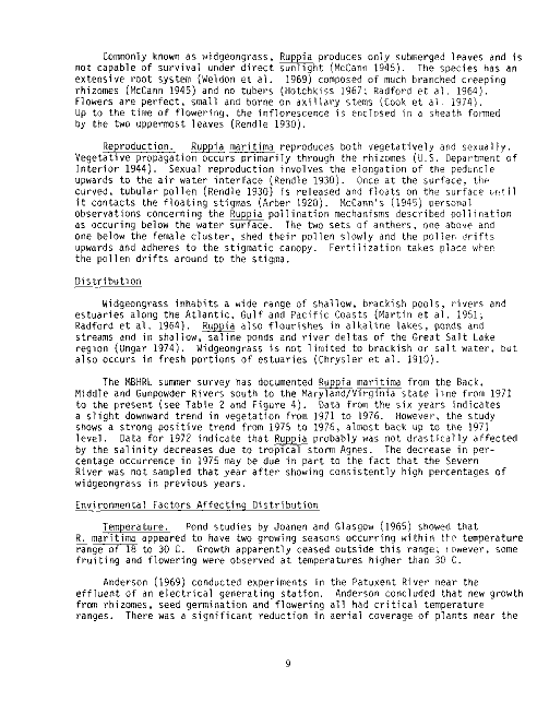
 Commonly known as widgeongrass, Ruppia produces only submerged leaves and is
not capable of survival under direct sunlight (McCann 1945). The species has an
extensive root system (Weldon et al. 1969) composed of much branched creeping
rhizomes (McCann 1945) and no tubers (Hotchkiss 1967; Radford et al. 1964).
Flowers are perfect, small and borne on axillary stems (Cook et al. 1974).
Up to the time of flowering, the inflorescence is enclosed in a sheath formed
by the two uppermost leaves (Rendle 1930).
Reproduction. Ruppia maritima reproduces both vegetatively and sexually.
Vegetative propagation occurs primarily through the rhizomes (U.S. Department of
Interior 1944). Sexual reproduction involves the elongation of the peduncle
upwards to the air water interface (Rendle 1930). Once at the surface, the
curved, tubular pollen (Rendle 1930) is released and floats on the surface until
it contacts the floating stigmas (Arber 1920). McCann's (1945) personal
observations concerning the Ruppia pollination mechanisms described pollination
as occuring below the water surface. The two sets of anthers, one above and
one below the female cluster, shed their pollen slowly and the pollen drifts
upwards and adheres to the stigmatic canopy. Fertilization takes place when
the pollen drifts around to the stigma.
Distribution
Widgeongrass inhabits a wide range of shallow, brackish pools, rivers and
estuaries along the Atlantic, Gulf and Pacific Coasts (Martin et al. 1951;
Radford et al. 1964). Ruppia also flourishes in alkaline lakes, ponds and
streams and in shallow, saline ponds and river deltas of the Great Salt Lake
region (Ungar 1974). Widgeongrass is not limited to brackish or salt water, but
also occurs in fresh portions of estuaries (Chrysler et al. 1910).
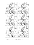
The MBHRL summer survey has documented Ruppia maritima from the Back,
Middle and Gunpowder Rivers south to the Maryland/Virginia state line from 1971
to the present (see Table 2 and Figure 4). Data from the six years indicates
a slight downward trend in vegetation from 1971 to 1976. However, the study
shows a strong positive trend from 1975 to 1976, almost back up to the 1971
level. Data for 1972 indicate that Ruppia probably was not drastically affected
by the salinity decreases due to tropical storm Agnes. The decrease in per-
centage occurrence in 1975 may be due in part to the fact that the Severn
River was not sampled that year after showing consistently high percentages of
widgeongrass in previous years.
Environmental Factors Affecting Distribution
Temperature. Pond studies by Joanen and Glasgow (1965) showed that
R. maritima appeared to have two growing seasons occurring within the temperature
range of 18 to 30 C. Growth apparently ceased outside this range; However, some
fruiting and flowering were observed at temperatures higher than 30 C.
Anderson (1969) conducted experiments in the Patuxent River near the
effluent of an electrical generating station. Anderson concluded that new growth
from rhizomes, seed germination and flowering all had critical temperature
ranges. There was a significant reduction in aerial coverage of plants near the
image:
Commonly known as widgeongrass, Ruppia produces only submerged leaves and is
not capable of survival under direct sunlight (McCann 1945). The species has an
extensive root system (Weldon et al. 1969) composed of much branched creeping
rhizomes (McCann 1945) and no tubers (Hotchkiss 1967; Radford et al. 1964).
Flowers are perfect, small and borne on axillary stems (Cook et al. 1974).
Up to the time of flowering, the inflorescence is enclosed in a sheath formed
by the two uppermost leaves (Rendle 1930).
Reproduction. Ruppia maritima reproduces both vegetatively and sexually.
Vegetative propagation occurs primarily through the rhizomes (U.S. Department of
Interior 1944). Sexual reproduction involves the elongation of the peduncle
upwards to the air water interface (Rendle 1930). Once at the surface, the
curved, tubular pollen (Rendle 1930) is released and floats on the surface until
it contacts the floating stigmas (Arber 1920). McCann's (1945) personal
observations concerning the Ruppia pollination mechanisms described pollination
as occuring below the water surface. The two sets of anthers, one above and
one below the female cluster, shed their pollen slowly and the pollen drifts
upwards and adheres to the stigmatic canopy. Fertilization takes place when
the pollen drifts around to the stigma.
Distribution
Widgeongrass inhabits a wide range of shallow, brackish pools, rivers and
estuaries along the Atlantic, Gulf and Pacific Coasts (Martin et al. 1951;
Radford et al. 1964). Ruppia also flourishes in alkaline lakes, ponds and
streams and in shallow, saline ponds and river deltas of the Great Salt Lake
region (Ungar 1974). Widgeongrass is not limited to brackish or salt water, but
also occurs in fresh portions of estuaries (Chrysler et al. 1910).
The MBHRL summer survey has documented Ruppia maritima from the Back,
Middle and Gunpowder Rivers south to the Maryland/Virginia state line from 1971
to the present (see Table 2 and Figure 4). Data from the six years indicates
a slight downward trend in vegetation from 1971 to 1976. However, the study
shows a strong positive trend from 1975 to 1976, almost back up to the 1971
level. Data for 1972 indicate that Ruppia probably was not drastically affected
by the salinity decreases due to tropical storm Agnes. The decrease in per-
centage occurrence in 1975 may be due in part to the fact that the Severn
River was not sampled that year after showing consistently high percentages of
widgeongrass in previous years.
Environmental Factors Affecting Distribution
Temperature. Pond studies by Joanen and Glasgow (1965) showed that
R. maritima appeared to have two growing seasons occurring within the temperature
range of 18 to 30 C. Growth apparently ceased outside this range; However, some
fruiting and flowering were observed at temperatures higher than 30 C.
Anderson (1969) conducted experiments in the Patuxent River near the
effluent of an electrical generating station. Anderson concluded that new growth
from rhizomes, seed germination and flowering all had critical temperature
ranges. There was a significant reduction in aerial coverage of plants near the
image:
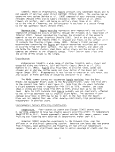 Table 2. Percent of sampling stations showing occurrence of
Ruppia maritima, Maryland Chesapeake Bay, 1971-1976a
Area
Code
1
2
3
4
5
6
7
8
9
10
11
12
13
14
15
16
17
18
19
20
21
22
23
24
25
26
Number of stations
River system
Elk 4 Bohemia
Rivers
Sassafras River
Howell & Swan
Points
Eastern Bay
Choptank River
Little Choptank
River
James Island &
Honga River
Honga River
Bloodsworth Is.
Susquehanna
Flats
Fishing Bay
Nanticoke &
vJicomico Rivers
Manokin River
Patapsco River
Big & Little
Annemessex Rivers
Gunpowder & Bush
River Headwaters
Pocomoke Sound
(Maryland)
Magothy River
Severn River
Patuxent River
Back, Middle &
Gunpowder Rivers
Curtis & Cove
Points
South, West 8
Rhode Rivers
Chester River
Love & Kent
Points
Smith Island
(Maryland)
Total
1971
0
0
0
23.40
23.33
15.79
17.65
30.00
20.00
0
8.00
0
20.00
0
45.00
0
9.09
8.33
33.33
-
4.55
0
0
27.78
0
47.06
14.74
1972
0
0
0
30.23
31.03
10.53
8.82
23.33
2.27
0
0
0
13.33
0
15.00
0
0
0
20.00
4.26
0
0
0
11.11
0
27.27
9.92
1973
0
0
0
23.40
10.53
0
2.94
10.00
8.70
0
0
0
6.67
0
25.00
0
0
0
13.33
-
0
0
0
8.82
0
16.67
6.04
1974
0
0
0
34.04
24.14
0
5.88
16.67
4.65
0
0
0
13.33
0
31.58
0
-
8.33
26.67
2.00
0
0
0
2.94
12.50
29.41
9.84
1975
0
0
0
17.39
1.72
0
5.88
10.34
4.65
0
0
0
7.14
-
16.67
_
5.00
-
-
0
0
0
0
11.11
0
5.56
4.69
1976
0
0
0
37.78
39.29
15.79
8.82
13.79
2.22
0
0
0
6.67
0
25.00
0
4.55
0
15.38
2.04
0
0
12.50
14.29
0
35.29
11.46
71
15
10
12
47
60
19
34
30
40
27
25
30
15
21
20
9
22
12
15
50
22
20
8
36
8
17
624
72
16
10
6
43
58
19
34
30
44
37
25
30
15
20
20
8
20
12
15
47
22
19
10
36
8
11
615
73
16
10
12
47
57
19
34
30
46
37
25
30
15
21
20
7
21
12
15
50
22
19
10
34
8
12
629
/4
16
10
12
47
58
19
34
30
43
37
25
30
15
21
19
9
-
12
15
50
22
19
8
34
8
17
610
7b
16
10
12
46
57
19
34
29
43
36
24
30
14
-
18
_
20
-
-
47
22
6
8
36
8
17
553
76
16
10
12
45
56
19
34
29
45
35
25
30
15
21
20
9
22
12
13
49
22
21
8
35
8
17
628
a
U.S. Fish and Wildlife Service Migratory Bird and Habitat Research Laboratory, 1976
10
image:
Table 2. Percent of sampling stations showing occurrence of
Ruppia maritima, Maryland Chesapeake Bay, 1971-1976a
Area
Code
1
2
3
4
5
6
7
8
9
10
11
12
13
14
15
16
17
18
19
20
21
22
23
24
25
26
Number of stations
River system
Elk 4 Bohemia
Rivers
Sassafras River
Howell & Swan
Points
Eastern Bay
Choptank River
Little Choptank
River
James Island &
Honga River
Honga River
Bloodsworth Is.
Susquehanna
Flats
Fishing Bay
Nanticoke &
vJicomico Rivers
Manokin River
Patapsco River
Big & Little
Annemessex Rivers
Gunpowder & Bush
River Headwaters
Pocomoke Sound
(Maryland)
Magothy River
Severn River
Patuxent River
Back, Middle &
Gunpowder Rivers
Curtis & Cove
Points
South, West 8
Rhode Rivers
Chester River
Love & Kent
Points
Smith Island
(Maryland)
Total
1971
0
0
0
23.40
23.33
15.79
17.65
30.00
20.00
0
8.00
0
20.00
0
45.00
0
9.09
8.33
33.33
-
4.55
0
0
27.78
0
47.06
14.74
1972
0
0
0
30.23
31.03
10.53
8.82
23.33
2.27
0
0
0
13.33
0
15.00
0
0
0
20.00
4.26
0
0
0
11.11
0
27.27
9.92
1973
0
0
0
23.40
10.53
0
2.94
10.00
8.70
0
0
0
6.67
0
25.00
0
0
0
13.33
-
0
0
0
8.82
0
16.67
6.04
1974
0
0
0
34.04
24.14
0
5.88
16.67
4.65
0
0
0
13.33
0
31.58
0
-
8.33
26.67
2.00
0
0
0
2.94
12.50
29.41
9.84
1975
0
0
0
17.39
1.72
0
5.88
10.34
4.65
0
0
0
7.14
-
16.67
_
5.00
-
-
0
0
0
0
11.11
0
5.56
4.69
1976
0
0
0
37.78
39.29
15.79
8.82
13.79
2.22
0
0
0
6.67
0
25.00
0
4.55
0
15.38
2.04
0
0
12.50
14.29
0
35.29
11.46
71
15
10
12
47
60
19
34
30
40
27
25
30
15
21
20
9
22
12
15
50
22
20
8
36
8
17
624
72
16
10
6
43
58
19
34
30
44
37
25
30
15
20
20
8
20
12
15
47
22
19
10
36
8
11
615
73
16
10
12
47
57
19
34
30
46
37
25
30
15
21
20
7
21
12
15
50
22
19
10
34
8
12
629
/4
16
10
12
47
58
19
34
30
43
37
25
30
15
21
19
9
-
12
15
50
22
19
8
34
8
17
610
7b
16
10
12
46
57
19
34
29
43
36
24
30
14
-
18
_
20
-
-
47
22
6
8
36
8
17
553
76
16
10
12
45
56
19
34
29
45
35
25
30
15
21
20
9
22
12
13
49
22
21
8
35
8
17
628
a
U.S. Fish and Wildlife Service Migratory Bird and Habitat Research Laboratory, 1976
10
image:
 1973
1975
Figure 4. Distribution of Ruppia maritima, Maryland Chesapeake Bay,
1971-1976
11
image:
1973
1975
Figure 4. Distribution of Ruppia maritima, Maryland Chesapeake Bay,
1971-1976
11
image:
 : : • •'•" iidl temperature may have been reached
for --•• - •. - -s!T'ftY'ture was determined to be 45 C.
^.•' A
'• -jrant of an extremely broad salinity
rancc .'"••. . • •'.••,. , .ncrqed aquatics because it can also
loie'vH- ,- . i-.-in<j dehydrated or hydro!ized (Ungar 1974;
-'•dfvh has been conducted to determine
' ' •••.!'- Kupjiju Steenis (1970) established a
ten:-;.:ii . . .',.j'8ss, Anderson (1972) determined a
Sai-rp:.- •• ' . , : !»pt. McMillan (1974) and Osterhaut
fiGU*'' ;; •"• , •< r-iinpd indefinitely in either tapwater
',.( r • .; -.'.-', i'-.uo the flowering of R. maritima
(Men-1 , I--:. '. -. . , ,r,; confined to lower salinity levels with
seed ;r:- = , - . • ••;-•'' pot to tapwater.
'-.:_:•,'r.. • : • prefer soft bottom muds (Anderson 1972)
;/eral feet (U.S. Department of Interior
; • ' : • ;:u|jj_iji marrti_ina_ beds growing on shallow
-.: • •'. ','ers and streams.
; >! extensive studies in Louisiana, Joanen and
- • of iight, depth and turbidity on Ruppia
' .;,,><r'\itory analysis was determined to occur at
., ureas where thick algal mats covered the
: ' -^itright, Ruppia plants were visibly weakened.
••-.••• nor'iMul to young plants prior to the stems
• <i:-;'»:; t} ranges showed Ruppia to develop best
• •; :-: small ponds. Experimental ponds with
• -< TJ. 1. ;:- :,o 108 ppm) could not support continuing
..,:..!•- :•,, r>>e plants reaching the surface, turbidity
and Glasgow (1965) concluded from
Ljula1* water fluctuation was the single
f?nt or elimination of widgeongrass.
sunlight penetration and provided long
-!--'ined that wave action limited the
T.ochdnic.al damage or by causing high
(1945) (ietermined that the branch tops
.'O a;:tidn. These detached fragments
ifna has shown a high tolerance to boron
r 850 ppm (Sculthorpe 1967). Ruppia
;e, sulphate, phosphorus and sodium
•s (Joanen and Glasgow 1965) poor
iih average of 177 ppm phosphorus
?vel or 120 ppm. Toxic levels were
ined "...no correlation between plant
any time inhibited plant growth."(p.13)
.o
image:
: : • •'•" iidl temperature may have been reached
for --•• - •. - -s!T'ftY'ture was determined to be 45 C.
^.•' A
'• -jrant of an extremely broad salinity
rancc .'"••. . • •'.••,. , .ncrqed aquatics because it can also
loie'vH- ,- . i-.-in<j dehydrated or hydro!ized (Ungar 1974;
-'•dfvh has been conducted to determine
' ' •••.!'- Kupjiju Steenis (1970) established a
ten:-;.:ii . . .',.j'8ss, Anderson (1972) determined a
Sai-rp:.- •• ' . , : !»pt. McMillan (1974) and Osterhaut
fiGU*'' ;; •"• , •< r-iinpd indefinitely in either tapwater
',.( r • .; -.'.-', i'-.uo the flowering of R. maritima
(Men-1 , I--:. '. -. . , ,r,; confined to lower salinity levels with
seed ;r:- = , - . • ••;-•'' pot to tapwater.
'-.:_:•,'r.. • : • prefer soft bottom muds (Anderson 1972)
;/eral feet (U.S. Department of Interior
; • ' : • ;:u|jj_iji marrti_ina_ beds growing on shallow
-.: • •'. ','ers and streams.
; >! extensive studies in Louisiana, Joanen and
- • of iight, depth and turbidity on Ruppia
' .;,,><r'\itory analysis was determined to occur at
., ureas where thick algal mats covered the
: ' -^itright, Ruppia plants were visibly weakened.
••-.••• nor'iMul to young plants prior to the stems
• <i:-;'»:; t} ranges showed Ruppia to develop best
• •; :-: small ponds. Experimental ponds with
• -< TJ. 1. ;:- :,o 108 ppm) could not support continuing
..,:..!•- :•,, r>>e plants reaching the surface, turbidity
and Glasgow (1965) concluded from
Ljula1* water fluctuation was the single
f?nt or elimination of widgeongrass.
sunlight penetration and provided long
-!--'ined that wave action limited the
T.ochdnic.al damage or by causing high
(1945) (ietermined that the branch tops
.'O a;:tidn. These detached fragments
ifna has shown a high tolerance to boron
r 850 ppm (Sculthorpe 1967). Ruppia
;e, sulphate, phosphorus and sodium
•s (Joanen and Glasgow 1965) poor
iih average of 177 ppm phosphorus
?vel or 120 ppm. Toxic levels were
ined "...no correlation between plant
any time inhibited plant growth."(p.13)
.o
image:
 Soil pH was not determined to be a limiting factor for Ruppia maritime growth;
plants grew vigorously in both high and low pH soils.
Susceptibility. Ruppia maritima has not been utilized extensively in
experiments to determine relative toxicity levels to various herbicides. A
possible explanation for this lack of information may be the recognized impor-
tance of Ruppia as waterfowl food. Further, the majority of the herbicide
toxicity experiments have been conducted in a fresh water media. Ruppia is not
often documented as a fresh water inhabitant.
Table 3 lists those herbicides documented by the U.S. Department of Agri-
culture for controlling
Table 3. Effects of certain aquatic herbicides on Ruppia maritima
Herbicide Application (ppm) Control
Sodium arsenite 1 Promising
Endothall, DOS 1.5 None
2 10 %
Acrolein 5.6 to 6.8 Good
aLawrence and Hollingsworth 1969.
CIBA-GEIGY (personal communication 1977) has not included Ruppia maritima on
their label for Aquazine (simazine). Their only information concerning Ruppia
refers to complete control with Aquazine at 1.0 ppm in a North Carolina lake.
Similar control could probably be expected with an atrazine concentration of
0.25 to 0.50 ppm.
Productivity
There is a scarcity of information available concerning productivity of
Ruppia maritima in the Chesapeake Bay. Anderson (1966) was able to compare
primary productivity of Ruppia between the Patuxent River and Chincoteague Bay
He found Ruppia to be considerably more productive in the Patuxent River (800 g/m2
average mean dry weight)than in Chincoteague Bay (250 g/m2 average mean dry
weight). The height of the growing season for Ruppia in Chincoteague Bay seemed
to occur from about the middle of June to the end of July. Growth did not
necessarily cease when the elongating stems reach the surface, so that leaf ex-
tension and expansion remained possible.
Consumer Utilization
Ruppia maritima is rivaled only by Zostera marina in importance to waterfowl
(Bourn 1935). Widgeongrassserves as food for numerous species of ducks, coots,
13
image:
Soil pH was not determined to be a limiting factor for Ruppia maritime growth;
plants grew vigorously in both high and low pH soils.
Susceptibility. Ruppia maritima has not been utilized extensively in
experiments to determine relative toxicity levels to various herbicides. A
possible explanation for this lack of information may be the recognized impor-
tance of Ruppia as waterfowl food. Further, the majority of the herbicide
toxicity experiments have been conducted in a fresh water media. Ruppia is not
often documented as a fresh water inhabitant.
Table 3 lists those herbicides documented by the U.S. Department of Agri-
culture for controlling
Table 3. Effects of certain aquatic herbicides on Ruppia maritima
Herbicide Application (ppm) Control
Sodium arsenite 1 Promising
Endothall, DOS 1.5 None
2 10 %
Acrolein 5.6 to 6.8 Good
aLawrence and Hollingsworth 1969.
CIBA-GEIGY (personal communication 1977) has not included Ruppia maritima on
their label for Aquazine (simazine). Their only information concerning Ruppia
refers to complete control with Aquazine at 1.0 ppm in a North Carolina lake.
Similar control could probably be expected with an atrazine concentration of
0.25 to 0.50 ppm.
Productivity
There is a scarcity of information available concerning productivity of
Ruppia maritima in the Chesapeake Bay. Anderson (1966) was able to compare
primary productivity of Ruppia between the Patuxent River and Chincoteague Bay
He found Ruppia to be considerably more productive in the Patuxent River (800 g/m2
average mean dry weight)than in Chincoteague Bay (250 g/m2 average mean dry
weight). The height of the growing season for Ruppia in Chincoteague Bay seemed
to occur from about the middle of June to the end of July. Growth did not
necessarily cease when the elongating stems reach the surface, so that leaf ex-
tension and expansion remained possible.
Consumer Utilization
Ruppia maritima is rivaled only by Zostera marina in importance to waterfowl
(Bourn 1935). Widgeongrassserves as food for numerous species of ducks, coots,
13
image:
 geese, grebes, swans, marsh and shore birds and game birds of the Atlantic,
Pacific and Gulf Coasts (Sculthorpe 1967; Martin and Uhler 1939). Studies of
the upper Chesapeake Bay area over the period 1959 to 1968 (Rawls in press)
showed Ruppia Maritima to have the highest frequency-of-use rate for the water-
fowl and plant species studied. Out of 1,179 geese, dabbling duck, diving duck
and Meganser gizzards utilized during the survey, 363 birds (30.79 percent) con-
tained widgeongrass plant parts. Volumetric analysis rated Ruppia third after
Zea mays and Potamogeton perfoliatus.
A study performed in the 1930s (Cottam 1934c) on the gullets of 3,499 North
American inland plant feeding ducks, included Ruppia Maritima in the list of
aquatic plants having the greatest food value to Nyroca and ruddy ducks. Water-
fowl were found to have eaten all parts of the Ruppia plants. Pond studies in
Louisiana (Joanen and Glasgow 1965) showed waterfowl utilization of Ruppia so
heavy as to consume entire plant stands.
Ruppia beds are also used as nursery grounds (Sculthorpe 1967) and as a fish
spawning medium and cover for marine organisms (Kerwin 1975b). Sculthorpe (1967)
also considered Ruppia stands of great importance to fish as a food and shade
source.
Economic Uses and Problems
Impoundments. Baldwin (1967), in studying the use of impoundments for the
management of waterfowl, concluded that when considering all types of impound-
ments, Ruppia maritima ponds probably provided more waterfowl food with the least
amount of management. Iii creating impoundments, Baldwin suggested that the fol-
lowing conditions would be delterious to Ruppia propagation: stained, acidic
water; excessive upland runoff; surplus fresh water; silt and detritus; and
organically stained water. The relatively high salinity tolerance of Ruppia
allows for the prevention of rapid changes caused by natural plant succession
and invasion by fresh water pests such as cattail (Typha spp.) (Ball 1965).
MYRIOPHYLLUM SPICATUM1
Biology
General Vegetative Morphology. Eurasian watermilfoil (Myriophyllum
spicatum) belongs to the order Hippuridales, family Haloragaceae (Takhtajan 1969).
The plant was first decribed by Linnaeus in 1953 (Anderson et al. 1965). Dis-
agreement persists in the literature as to the proper taxonomic relationship to
a very similarly appearing species, Myriophyllum exalbescens. M. spicatum is
closely related to M. exalbescens. but the latter species is found mostly in
glaciated areas (Steenis and Stotts 1961). Beaven (1962), in his summary report
included a suggestion by Dr. Paul Springer that new reports of M. spicatum in
Special contribution from Charles K. Rawls, University of Maryland Center for
Environmental and Estuarine Studies, Chesapeake Biological Laboratory.
14
image:
geese, grebes, swans, marsh and shore birds and game birds of the Atlantic,
Pacific and Gulf Coasts (Sculthorpe 1967; Martin and Uhler 1939). Studies of
the upper Chesapeake Bay area over the period 1959 to 1968 (Rawls in press)
showed Ruppia Maritima to have the highest frequency-of-use rate for the water-
fowl and plant species studied. Out of 1,179 geese, dabbling duck, diving duck
and Meganser gizzards utilized during the survey, 363 birds (30.79 percent) con-
tained widgeongrass plant parts. Volumetric analysis rated Ruppia third after
Zea mays and Potamogeton perfoliatus.
A study performed in the 1930s (Cottam 1934c) on the gullets of 3,499 North
American inland plant feeding ducks, included Ruppia Maritima in the list of
aquatic plants having the greatest food value to Nyroca and ruddy ducks. Water-
fowl were found to have eaten all parts of the Ruppia plants. Pond studies in
Louisiana (Joanen and Glasgow 1965) showed waterfowl utilization of Ruppia so
heavy as to consume entire plant stands.
Ruppia beds are also used as nursery grounds (Sculthorpe 1967) and as a fish
spawning medium and cover for marine organisms (Kerwin 1975b). Sculthorpe (1967)
also considered Ruppia stands of great importance to fish as a food and shade
source.
Economic Uses and Problems
Impoundments. Baldwin (1967), in studying the use of impoundments for the
management of waterfowl, concluded that when considering all types of impound-
ments, Ruppia maritima ponds probably provided more waterfowl food with the least
amount of management. Iii creating impoundments, Baldwin suggested that the fol-
lowing conditions would be delterious to Ruppia propagation: stained, acidic
water; excessive upland runoff; surplus fresh water; silt and detritus; and
organically stained water. The relatively high salinity tolerance of Ruppia
allows for the prevention of rapid changes caused by natural plant succession
and invasion by fresh water pests such as cattail (Typha spp.) (Ball 1965).
MYRIOPHYLLUM SPICATUM1
Biology
General Vegetative Morphology. Eurasian watermilfoil (Myriophyllum
spicatum) belongs to the order Hippuridales, family Haloragaceae (Takhtajan 1969).
The plant was first decribed by Linnaeus in 1953 (Anderson et al. 1965). Dis-
agreement persists in the literature as to the proper taxonomic relationship to
a very similarly appearing species, Myriophyllum exalbescens. M. spicatum is
closely related to M. exalbescens. but the latter species is found mostly in
glaciated areas (Steenis and Stotts 1961). Beaven (1962), in his summary report
included a suggestion by Dr. Paul Springer that new reports of M. spicatum in
Special contribution from Charles K. Rawls, University of Maryland Center for
Environmental and Estuarine Studies, Chesapeake Biological Laboratory.
14
image:
 the Northern United States may have been the results of misidentification of
M. exalbescens. Love (1961) maintained that differences between the two species
are so pronounced that they can confidently be considered to be separate species.
The Terminology Committee of the Weed Society of America (Klingman 1962) has
given approval to common names of Eurasian watermilfoil for M. spicatum and to
northern watermilfoil for M_. exalbescens.
Myriophyllum spicatum is an aquatic perennial with verticilliate submerged
leaves which are pinnatified (Southwick 1972) (see Figure 5). Springer (1959)
described milfoil as generally having leaves with 14 to 21 pairs of upward curv-
ing, threadlike divisions and stems that are greenish and remain this color when
dry. Springer et al. (1961) compared milfoil leaves to weathered, watersoaked
feathers. M_. spicatum is much branching, variable in growth under various condi-
tions and with leaflets near the flowering tips more numerous (usually 13 or
more) than in other milfoil species (Stotts 1961). The leaflets are about 1.8
cm long (Haven 1961). The flowers are axillary and monoecious.
Reproduction. Patten (1956) studied the flowering and reproductive cycles
of the perennial M_. spicatum in the shallow, alkaline, eutrophic New Jersey
Lake Musconetcong. Flowering began in late May and continued until early October
with the earliest flowering occurring in the shallower lake depths.
Patten (1955) described the sexual reproductive cycle of milfoil. Upper
flowers are staminate, the lower pistillate, both are sessile in axils of strong
bracts and the sexual flowering cycle is brief. The spike axis elongates, then
pollination follows and finally resubmergence. Pollination is aerial, but mil-
foil is not self pollinated; the stigmas ripen in advance of the stamens. The
achenes sink to the bottom, exhibit high viability (as much as 80 to 90 percent)
and can remain viable for as much as 10 years. Germination is generally delayed,
but is speeded up by freezing and drying. Seed capacity to germinate increases
with age.
Milfoil reproduces most effectively by way of vegetative reproduction
through fragmentation, rhizomes and axillary buds (Patten 1956). In the Chesa-
peake Bay, Haven (1961) found that foliage of this perennial plant died back in
the late fall, was renewed from roots and reached maximum growth in late summer.
Springer (1959) found reproduction by fragmentation in the fall, by seeding (no
time given) and by budding or sprouting in the spring.
Annual fluctuations in submerged aquatic vegetation species is natural and
presents a continually changing picture. Some species, such as Eurasian water-
milfoil, seem to be more subject to changes in their range and density than other
species. In most areas, milfoil has two growth-surge periods during the growing
season. To keep abreast of such changes, two or three surveys of vegetation beds
should be made annually (Rawls 1971a_).
Distribution
There is some controversy as to where milfoil was originally introduced on
the East Coast of the United States. Beaven (1962) noted that the plant oriainal-
ly may have been introducted between 1880 and 1890 when ships coming from Europe
15
image:
the Northern United States may have been the results of misidentification of
M. exalbescens. Love (1961) maintained that differences between the two species
are so pronounced that they can confidently be considered to be separate species.
The Terminology Committee of the Weed Society of America (Klingman 1962) has
given approval to common names of Eurasian watermilfoil for M. spicatum and to
northern watermilfoil for M_. exalbescens.
Myriophyllum spicatum is an aquatic perennial with verticilliate submerged
leaves which are pinnatified (Southwick 1972) (see Figure 5). Springer (1959)
described milfoil as generally having leaves with 14 to 21 pairs of upward curv-
ing, threadlike divisions and stems that are greenish and remain this color when
dry. Springer et al. (1961) compared milfoil leaves to weathered, watersoaked
feathers. M_. spicatum is much branching, variable in growth under various condi-
tions and with leaflets near the flowering tips more numerous (usually 13 or
more) than in other milfoil species (Stotts 1961). The leaflets are about 1.8
cm long (Haven 1961). The flowers are axillary and monoecious.
Reproduction. Patten (1956) studied the flowering and reproductive cycles
of the perennial M_. spicatum in the shallow, alkaline, eutrophic New Jersey
Lake Musconetcong. Flowering began in late May and continued until early October
with the earliest flowering occurring in the shallower lake depths.
Patten (1955) described the sexual reproductive cycle of milfoil. Upper
flowers are staminate, the lower pistillate, both are sessile in axils of strong
bracts and the sexual flowering cycle is brief. The spike axis elongates, then
pollination follows and finally resubmergence. Pollination is aerial, but mil-
foil is not self pollinated; the stigmas ripen in advance of the stamens. The
achenes sink to the bottom, exhibit high viability (as much as 80 to 90 percent)
and can remain viable for as much as 10 years. Germination is generally delayed,
but is speeded up by freezing and drying. Seed capacity to germinate increases
with age.
Milfoil reproduces most effectively by way of vegetative reproduction
through fragmentation, rhizomes and axillary buds (Patten 1956). In the Chesa-
peake Bay, Haven (1961) found that foliage of this perennial plant died back in
the late fall, was renewed from roots and reached maximum growth in late summer.
Springer (1959) found reproduction by fragmentation in the fall, by seeding (no
time given) and by budding or sprouting in the spring.
Annual fluctuations in submerged aquatic vegetation species is natural and
presents a continually changing picture. Some species, such as Eurasian water-
milfoil, seem to be more subject to changes in their range and density than other
species. In most areas, milfoil has two growth-surge periods during the growing
season. To keep abreast of such changes, two or three surveys of vegetation beds
should be made annually (Rawls 1971a_).
Distribution
There is some controversy as to where milfoil was originally introduced on
the East Coast of the United States. Beaven (1962) noted that the plant oriainal-
ly may have been introducted between 1880 and 1890 when ships coming from Europe
15
image:
 (copied from Hotchkiss 1967)
Figure 5. Eurasian watermiIfoi ! (Hyr1ophy11 urn spicatum)
16
image:
(copied from Hotchkiss 1967)
Figure 5. Eurasian watermiIfoi ! (Hyr1ophy11 urn spicatum)
16
image:
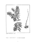 dumped their ballast. Others (Bayley et al. in press; Steenis 1970; Rawls
1964, 1975; Steenis et al. 1962; Springer et al. 1961; Elser 1966; Steenis
et al. 1967) have traced the early history of milfoil back to various dates
ranging from 1895 to 1902.
From the turn of the century until the 1950s, milfoil was found sporadically
from the C & D Canal in Baltimore south into North Carolina. However, according
to Virginia Institute of Marine Science (VIMS), Chesapeake Bay Laboratory
(CBL) and Migratory Bird and Habitat Research Laboratory (MBHRL) personnel,
rapid spread did not begin until around 1954. By 1959 live fragments of milfoil
could be found floating all over the Bay (Steenis et al. 1962). Bay acreage
infested by milfoil increased from 20,200 ha in 1960 to 40,500 ha in 1961, An
example of the rapidity with which milfoil infested the Bay was seen on the
Susquehanna Flats where a survey showed that the percentage of established
transect stations with milfoil was 0 in 1957, 1 percent in 1958, 47 percent in
1959, 94 percent in 1960, 71 percent in 1961 and 88 percent during another 1961
sampling of the same stations (Steenis et al. 1962).
As dramatically as milfoil infested the Bay from about 1959 to 1965, it
declined just as rapidly. However, the decline was not uniform within the
entire Bay. From 1959 to 1960, there was a decrease in milfoil infested areas
in the Lower Machodoc Creek, Virginia, for no known reason (Stotts 1961).
Rawls (1968) described changes in one Potomac River tributary, the Wicomico
River. Milfoil was classed as abundant throughout the entire Wicomico River in
1964 and 1965. In 1966 it was abundant only in the upper portion of the river
above Mills Point and by 1967 was limited to a small acreage near Allan's Fresh
at the head of the river. However, in 1968, there were 80 ha where there had
been 5 ha in 1967, and along the western shore between the power line river
crossing and Chaptico Bay, rooted milfoil beds covered an estimated 300 to 400
ha in a continuous stretch. The previous year, for the entire Wicomico, the
estimate was less than 4 ha of milfoil.
Munro (1976b_) discussed the decrease in Chesapeake Bay aquatic vegetation
based on the 1971 to 1976 MBHRL survey (see Figure 6). Milfoil declined over
the six-year survey from 3.85 percent vegetated stations in 1971 to 0.96 percent
vegetated stations in 1976. In attempting to characterize the spectacular
invasion of the Chesapeake Bay by milfoil, Bayley et al. (in press) described
the milfoil spread on the Susquehanna Flats as a "wave phenomenon" from an
epicenter, spreading from the most optimal to the least optimal areas. At
first milfoil was co-dominant with Najas spp. and Vallisneria americana.
Bayley et al.(in press) further stated that milfoil stands tended to become
homogenic and discrete within three years, but later were structured to include
several species of SAV at various densities. In time the milfoil epidemic
receded and a new equilibrium was established. In theory an area is most
susceptible to an epidemic when, the natural ecosystems are disturbed, partic-
ularly by man.
The present (summer, 1977) statu of Eurasian milfoil in the Chesapeake
Bay is uncertain. The Susquehanna Flats Survey and the MBHRL Survey were
conducted over July and August. Unless tnese surveys uncover drastic changes
over 1976 populations, there will again be remnant stands and pockets of milfoil
in scattered areas of the upper Chesapeake Bay and its tributaries.
17
image:
dumped their ballast. Others (Bayley et al. in press; Steenis 1970; Rawls
1964, 1975; Steenis et al. 1962; Springer et al. 1961; Elser 1966; Steenis
et al. 1967) have traced the early history of milfoil back to various dates
ranging from 1895 to 1902.
From the turn of the century until the 1950s, milfoil was found sporadically
from the C & D Canal in Baltimore south into North Carolina. However, according
to Virginia Institute of Marine Science (VIMS), Chesapeake Bay Laboratory
(CBL) and Migratory Bird and Habitat Research Laboratory (MBHRL) personnel,
rapid spread did not begin until around 1954. By 1959 live fragments of milfoil
could be found floating all over the Bay (Steenis et al. 1962). Bay acreage
infested by milfoil increased from 20,200 ha in 1960 to 40,500 ha in 1961, An
example of the rapidity with which milfoil infested the Bay was seen on the
Susquehanna Flats where a survey showed that the percentage of established
transect stations with milfoil was 0 in 1957, 1 percent in 1958, 47 percent in
1959, 94 percent in 1960, 71 percent in 1961 and 88 percent during another 1961
sampling of the same stations (Steenis et al. 1962).
As dramatically as milfoil infested the Bay from about 1959 to 1965, it
declined just as rapidly. However, the decline was not uniform within the
entire Bay. From 1959 to 1960, there was a decrease in milfoil infested areas
in the Lower Machodoc Creek, Virginia, for no known reason (Stotts 1961).
Rawls (1968) described changes in one Potomac River tributary, the Wicomico
River. Milfoil was classed as abundant throughout the entire Wicomico River in
1964 and 1965. In 1966 it was abundant only in the upper portion of the river
above Mills Point and by 1967 was limited to a small acreage near Allan's Fresh
at the head of the river. However, in 1968, there were 80 ha where there had
been 5 ha in 1967, and along the western shore between the power line river
crossing and Chaptico Bay, rooted milfoil beds covered an estimated 300 to 400
ha in a continuous stretch. The previous year, for the entire Wicomico, the
estimate was less than 4 ha of milfoil.
Munro (1976b_) discussed the decrease in Chesapeake Bay aquatic vegetation
based on the 1971 to 1976 MBHRL survey (see Figure 6). Milfoil declined over
the six-year survey from 3.85 percent vegetated stations in 1971 to 0.96 percent
vegetated stations in 1976. In attempting to characterize the spectacular
invasion of the Chesapeake Bay by milfoil, Bayley et al. (in press) described
the milfoil spread on the Susquehanna Flats as a "wave phenomenon" from an
epicenter, spreading from the most optimal to the least optimal areas. At
first milfoil was co-dominant with Najas spp. and Vallisneria americana.
Bayley et al.(in press) further stated that milfoil stands tended to become
homogenic and discrete within three years, but later were structured to include
several species of SAV at various densities. In time the milfoil epidemic
receded and a new equilibrium was established. In theory an area is most
susceptible to an epidemic when, the natural ecosystems are disturbed, partic-
ularly by man.
The present (summer, 1977) statu of Eurasian milfoil in the Chesapeake
Bay is uncertain. The Susquehanna Flats Survey and the MBHRL Survey were
conducted over July and August. Unless tnese surveys uncover drastic changes
over 1976 populations, there will again be remnant stands and pockets of milfoil
in scattered areas of the upper Chesapeake Bay and its tributaries.
17
image:
 1971
1973
1975
\
\
Figure 6. Distribution of Myriophyllum spicatum, Maryland Chesapeake
Bay, 1971-1976
18
image:
1971
1973
1975
\
\
Figure 6. Distribution of Myriophyllum spicatum, Maryland Chesapeake
Bay, 1971-1976
18
image:
 Outside the Chesapeake Bay area, milfoil has also infested many lakes in
New York, New Jersey and Tennessee (Springer et al. 1961; Stotts 1961). Eurasian
watermilfoil is still a problem in the Kawartha Lake region of Ontario, Canada
(Steenis 1976). It also has become a nuisance in such areas of British Columbia
as Osoyoos and Kalamalka in Skaha and Okanagan Lakes (Newroth 1977). As one
would suspect from the name, it is native to Europe and Asia (Anonymous 1976),
and is widespread in Europe, Asia and parts of Africa (Springer 1959).
Eurasian watermilfoil is the chief submersed aquatic vegetation species in
company with redhead grass (Potamggeton perfoliatus) and sago pondweed
(Potamogeton pectinatus) in the Kiliyskaya Delta of the Russian Danube (Klokov
Zimbalevskaya 1974).Milfoil is also known to be in at least the middle
course of the Saale River of East Germany (Krausch 1976).
Environmental Factors Affecting Distribution
Temperature. Anderson (1964) and Anderson et al. (1965) found milfoil
growing in temperatures ranging from 0.1 to 30 C in the freshwater Twin Ponds.
Vigorously growing milfoil was even found under 25 cm of ice.
Titus et al. (1975) described temperature as a primary environmental
forcing function. In a production model, Titus et al. determined that a 10 C
increase stimulated a 10 percent increase in the peak standing crop.
In the reactor cooling reservior Par Pond, South Carolina, the distribution
of aquatic macrophytes was studied by Grace and Tilly (1976). The standing
crop of milfoil as measured by biomass, was most abundant at the warm station
(average maximum temperature was 23.8 C), was twice as high as the cold station
(maximum temperature was 2.2 C) and three times as high as the hot station
(maximum temperature was 26.3 C).
Salinity. Myriophyllum spicatum customarily inhabits fresh to brackish
waters. Under natural conditions, milfoil can be found in salinities ranging
from 0 to 20 ppt (Rawls 1964). At 20 ppt, Beaven (1960) found milfoil alive
during the summer, but plants exhibited little growth. Only the foliage
remaining at the growing tips was alive. From observations in the Chesapeake
Bay, Davis et al. (1974) commented that milfoil disappeared as salinities
increased to 13 or 14 ppt.
In laboratory studies, Boyer (1960bJ found milfoil to grow well in water
from 0 to 5 ppt. Springer (1959) determined that milfoil rooted best at 3.5 ppt.
As salinities were increased, milfoil growth decreased. Boyer (1960) proved
this experimentally; inhibition started at 10 ppt and became severe from 15 to
20 ppt. Haller et al. (1974) in similar experiments, found some toxicity to
occur in salinities from 10 to 13.3 ppt. At 16.6 ppt, plants died.
Leaf area, stem diameter and extent of flowering was found to decrease
as salinity increased, while flowering was delayed or non-existent with
sufficient salinity increases. When salinities increased above 15 ppt, stems
broke near the bottom and large floating mats of partially decayed plant material
formed (Anderson 1964).
19
image:
Outside the Chesapeake Bay area, milfoil has also infested many lakes in
New York, New Jersey and Tennessee (Springer et al. 1961; Stotts 1961). Eurasian
watermilfoil is still a problem in the Kawartha Lake region of Ontario, Canada
(Steenis 1976). It also has become a nuisance in such areas of British Columbia
as Osoyoos and Kalamalka in Skaha and Okanagan Lakes (Newroth 1977). As one
would suspect from the name, it is native to Europe and Asia (Anonymous 1976),
and is widespread in Europe, Asia and parts of Africa (Springer 1959).
Eurasian watermilfoil is the chief submersed aquatic vegetation species in
company with redhead grass (Potamggeton perfoliatus) and sago pondweed
(Potamogeton pectinatus) in the Kiliyskaya Delta of the Russian Danube (Klokov
Zimbalevskaya 1974).Milfoil is also known to be in at least the middle
course of the Saale River of East Germany (Krausch 1976).
Environmental Factors Affecting Distribution
Temperature. Anderson (1964) and Anderson et al. (1965) found milfoil
growing in temperatures ranging from 0.1 to 30 C in the freshwater Twin Ponds.
Vigorously growing milfoil was even found under 25 cm of ice.
Titus et al. (1975) described temperature as a primary environmental
forcing function. In a production model, Titus et al. determined that a 10 C
increase stimulated a 10 percent increase in the peak standing crop.
In the reactor cooling reservior Par Pond, South Carolina, the distribution
of aquatic macrophytes was studied by Grace and Tilly (1976). The standing
crop of milfoil as measured by biomass, was most abundant at the warm station
(average maximum temperature was 23.8 C), was twice as high as the cold station
(maximum temperature was 2.2 C) and three times as high as the hot station
(maximum temperature was 26.3 C).
Salinity. Myriophyllum spicatum customarily inhabits fresh to brackish
waters. Under natural conditions, milfoil can be found in salinities ranging
from 0 to 20 ppt (Rawls 1964). At 20 ppt, Beaven (1960) found milfoil alive
during the summer, but plants exhibited little growth. Only the foliage
remaining at the growing tips was alive. From observations in the Chesapeake
Bay, Davis et al. (1974) commented that milfoil disappeared as salinities
increased to 13 or 14 ppt.
In laboratory studies, Boyer (1960bJ found milfoil to grow well in water
from 0 to 5 ppt. Springer (1959) determined that milfoil rooted best at 3.5 ppt.
As salinities were increased, milfoil growth decreased. Boyer (1960) proved
this experimentally; inhibition started at 10 ppt and became severe from 15 to
20 ppt. Haller et al. (1974) in similar experiments, found some toxicity to
occur in salinities from 10 to 13.3 ppt. At 16.6 ppt, plants died.
Leaf area, stem diameter and extent of flowering was found to decrease
as salinity increased, while flowering was delayed or non-existent with
sufficient salinity increases. When salinities increased above 15 ppt, stems
broke near the bottom and large floating mats of partially decayed plant material
formed (Anderson 1964).
19
image:
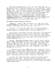 Biological stress induced by severe drought in 1933 to 1934 reduced most
vegetation in the lower Potomac River to remnant stands. Presumably this was
due to salt water intrusion which moved as far up the Potomac River as Mt.
Vernon.
Alkalinity, pH, C02, 02. Milfoil is generally absent in more acid waters
while the alkalinity of brackish waters favor growth (Steenis and Stotts 1961).
Eurasian watermilfoil has an affinity for alkaline waters (Patten 1956) and can
precipitate encrusting marl under highly calcareous conditions (Nichols 1975).
On August 1, 1962, near the mouth of the South River, Southwick (1972) obtained
pH readings from 7.2 to 8.9; free C02=0.00, phenolthalein alkalinity = 7.25 to
21.0. The readings were made as water temperatures rose from 25 C to 29 C.
Based on measurements obtained over a 13-hour tidal cycle in the Wicomico River
(Potomac River estuary) Anderson et al. (1965) concluded that a pH range from
5.8 to 9.7 and a low concentration of COa were not limiting factors. In field
studies, Rawls (1977) reported a pH range of 7.9 to 9.3 between June 24 and
October 16, in Chaptico Bay. Oxygen during the same period was measured from
5.6 to 9.9 ppm at the surface and 6.64 to 7.66 ppm at the bottom in milfoil
infested waters. Southwick (1972) stated that milfoil could survive in oxygen
depleted waters (no levels given).
Substrate. Studies by Patten (1956) in Lake Musconetcong, New Jersey,
correlated milfoil density to substrate particle size. Maximum density coin-
cided with fine organic ooze while minimum density was found in sand.
In the Chesapeake Bay, milfoil has generally been considered to grow best
in soft muck or sandy muck bottoms (Anderson 1972; Steenis et al. 1967;
Philipp and Brown 1965; Springer 1959). However, milfoil is capable of invading
hard sand in protected areas (Steenis and Stotts 1961) and in oyster beds
(Rawls 1964, 1965a_, 1975).
Light, Depth and Turbidity. The limiting or lethal extremes of depth,
turbidity and light as they apply to milfoil are not clear. The penetration
of light into water is directly proportional to both depth and turbidity, and
turbidity in turn is a reflection not only of sedimentation rates, but wave,
tidal and wind action, erosion, and a multiplicity of environmental factors
encountered under field conditions.
From a production study in Lake Wingra, Wisconsin, Titus et al. (1975)
concluded that light and temperature were primary environmental forcing
functions. Plant growth was limited in extremely turbid waters to 1.5 m, but
plants reaching the surface were able to slough off the lower leaves and thus
better adapt to turbid waters. Patten (1956) felt that in Lake Musconetcong,
New Jersey, where milfoil was found in waters to 2 m deep, water depth and
temperature were secondary in determining milfoil density. In studying the
relation of depth to temperature, Grace and Tilly (1976) looked at three stations
in a reactor cooling reservoir. Rooting depth was greater at the cold station
than the hot: 4 to 5 m at the cold; 4 m at the warm; and 3 m at the hot station.
Light penetration may have been partially responsible.
20
image:
Biological stress induced by severe drought in 1933 to 1934 reduced most
vegetation in the lower Potomac River to remnant stands. Presumably this was
due to salt water intrusion which moved as far up the Potomac River as Mt.
Vernon.
Alkalinity, pH, C02, 02. Milfoil is generally absent in more acid waters
while the alkalinity of brackish waters favor growth (Steenis and Stotts 1961).
Eurasian watermilfoil has an affinity for alkaline waters (Patten 1956) and can
precipitate encrusting marl under highly calcareous conditions (Nichols 1975).
On August 1, 1962, near the mouth of the South River, Southwick (1972) obtained
pH readings from 7.2 to 8.9; free C02=0.00, phenolthalein alkalinity = 7.25 to
21.0. The readings were made as water temperatures rose from 25 C to 29 C.
Based on measurements obtained over a 13-hour tidal cycle in the Wicomico River
(Potomac River estuary) Anderson et al. (1965) concluded that a pH range from
5.8 to 9.7 and a low concentration of COa were not limiting factors. In field
studies, Rawls (1977) reported a pH range of 7.9 to 9.3 between June 24 and
October 16, in Chaptico Bay. Oxygen during the same period was measured from
5.6 to 9.9 ppm at the surface and 6.64 to 7.66 ppm at the bottom in milfoil
infested waters. Southwick (1972) stated that milfoil could survive in oxygen
depleted waters (no levels given).
Substrate. Studies by Patten (1956) in Lake Musconetcong, New Jersey,
correlated milfoil density to substrate particle size. Maximum density coin-
cided with fine organic ooze while minimum density was found in sand.
In the Chesapeake Bay, milfoil has generally been considered to grow best
in soft muck or sandy muck bottoms (Anderson 1972; Steenis et al. 1967;
Philipp and Brown 1965; Springer 1959). However, milfoil is capable of invading
hard sand in protected areas (Steenis and Stotts 1961) and in oyster beds
(Rawls 1964, 1965a_, 1975).
Light, Depth and Turbidity. The limiting or lethal extremes of depth,
turbidity and light as they apply to milfoil are not clear. The penetration
of light into water is directly proportional to both depth and turbidity, and
turbidity in turn is a reflection not only of sedimentation rates, but wave,
tidal and wind action, erosion, and a multiplicity of environmental factors
encountered under field conditions.
From a production study in Lake Wingra, Wisconsin, Titus et al. (1975)
concluded that light and temperature were primary environmental forcing
functions. Plant growth was limited in extremely turbid waters to 1.5 m, but
plants reaching the surface were able to slough off the lower leaves and thus
better adapt to turbid waters. Patten (1956) felt that in Lake Musconetcong,
New Jersey, where milfoil was found in waters to 2 m deep, water depth and
temperature were secondary in determining milfoil density. In studying the
relation of depth to temperature, Grace and Tilly (1976) looked at three stations
in a reactor cooling reservoir. Rooting depth was greater at the cold station
than the hot: 4 to 5 m at the cold; 4 m at the warm; and 3 m at the hot station.
Light penetration may have been partially responsible.
20
image:
 In the Chesapeake Bay milfoil ius been found to require moderately high
light intensity, is sensitive to turbidity and grows in water more than 2 m deep,
if clear (Southwick 1972). Springer et al. (1961) reported milfoil in clear
water to 3.5 m deep at high tide, and in 1.8 to 2.1 m when the Secchi disc read-
ing was 0.8 m. Rawls (1964) found milfoil growing in clear waters from a few
centimeters deep to 2.7 m deep at mean low tide (tidal amplitude in the upper
Chesapeake Bay areas studied averaged about 0.5 m). Southwick (1967-1969) felt
that low light and turbidity might have been the main limiting factors for mil-
foil establishment in Back River at Baltimore. Rawls (1971bJ during field
studies in Chaptico Bay, found dense milfoil beds in waters where Secchi disc
readings ranged from 0.5 to 1.2 m. During the period of this study, carp-root-
ing action kept the water extremely turbid in fingers and small guts, but mil-
foil was present in moderate to heavy stands and extended to the surface at high
tide. A Secchi reading in these areas at such times of carp activity was about
7.5 cm.
Kerwin et al. (1975bJ assumed turbidity along with salinity to be major
limiting factors affecting the distribution and abundance of vascular aquatic
plants in the Chesapeake Bay. Rawls et al. (1975) pointed out such activities
as bank and upland erosion, construction, dredging, increased boating, stream
channelization and straightening and eul.rophication were contributing factors to
turbidity increases.
Current, Wind and Wave Action- Milfoil grows best in protected waters
but can withstand tidal fluctuations of 0.6 m (Springer 1959). Milfoil is vul-
nerable to strong tidal currents and wave action that might not affect other
native, rooted submersed aquatic vegetation species (Rawls et al. 1975). Severe
wave action limits milfoil establishment, but once established, milfoil helps
reduce wave effects (Stotts 1961).
Sedimentation. Grace and Tilly (1976) list Sculthorpe (1967) in their
literature cited, and attribute him with having generalized that milfoil is
likely to be eliminated from regions where suspended solids tend to settle at
high rates.
Nutrient Response. The growth of aquatic weeds, including Eurasian
watermilfoil, is promoted through enrichment of habitat waters by nutrient
materials, mainly nitrogen and phosphorous, The chief sources of these nutrients
are fertilizers, sewage effluents, disposal plants, overflow and seepage from
septic tanks, waste from pleasure craft and other vessels and migrating ducks
and geese (Elser 1966).
Dr. Clyde Reed pointed out (Beaven 1962) that in Maryland, all waters that
were heavily infested by milfoil received their runoff from limestone areas.
This was also true in T.V.A. lakes and other areas where milfoil was abundant.
With a reduction in coal mining in Pennsylvania, acid wastes finding their way
into the Susquehanna River at the head of the Chesapeake Bay decreased and cal-
cium ions sharply increased in recent years. This has favored growth of milfoil
in the upper Bay. John Gallagher reported (Beaven 1962) that the milfoil problem
was severe in northern New Jersey where the presence of iron was high. Anderson
(1964) found no significant increase in minerals in milfoil, despite mineral in-
creases in waters from which the milfoil was taken. He felt that milfoil could
use the bicarbonate ion directly from the wafer for its carbon source since
21
image:
In the Chesapeake Bay milfoil ius been found to require moderately high
light intensity, is sensitive to turbidity and grows in water more than 2 m deep,
if clear (Southwick 1972). Springer et al. (1961) reported milfoil in clear
water to 3.5 m deep at high tide, and in 1.8 to 2.1 m when the Secchi disc read-
ing was 0.8 m. Rawls (1964) found milfoil growing in clear waters from a few
centimeters deep to 2.7 m deep at mean low tide (tidal amplitude in the upper
Chesapeake Bay areas studied averaged about 0.5 m). Southwick (1967-1969) felt
that low light and turbidity might have been the main limiting factors for mil-
foil establishment in Back River at Baltimore. Rawls (1971bJ during field
studies in Chaptico Bay, found dense milfoil beds in waters where Secchi disc
readings ranged from 0.5 to 1.2 m. During the period of this study, carp-root-
ing action kept the water extremely turbid in fingers and small guts, but mil-
foil was present in moderate to heavy stands and extended to the surface at high
tide. A Secchi reading in these areas at such times of carp activity was about
7.5 cm.
Kerwin et al. (1975bJ assumed turbidity along with salinity to be major
limiting factors affecting the distribution and abundance of vascular aquatic
plants in the Chesapeake Bay. Rawls et al. (1975) pointed out such activities
as bank and upland erosion, construction, dredging, increased boating, stream
channelization and straightening and eul.rophication were contributing factors to
turbidity increases.
Current, Wind and Wave Action- Milfoil grows best in protected waters
but can withstand tidal fluctuations of 0.6 m (Springer 1959). Milfoil is vul-
nerable to strong tidal currents and wave action that might not affect other
native, rooted submersed aquatic vegetation species (Rawls et al. 1975). Severe
wave action limits milfoil establishment, but once established, milfoil helps
reduce wave effects (Stotts 1961).
Sedimentation. Grace and Tilly (1976) list Sculthorpe (1967) in their
literature cited, and attribute him with having generalized that milfoil is
likely to be eliminated from regions where suspended solids tend to settle at
high rates.
Nutrient Response. The growth of aquatic weeds, including Eurasian
watermilfoil, is promoted through enrichment of habitat waters by nutrient
materials, mainly nitrogen and phosphorous, The chief sources of these nutrients
are fertilizers, sewage effluents, disposal plants, overflow and seepage from
septic tanks, waste from pleasure craft and other vessels and migrating ducks
and geese (Elser 1966).
Dr. Clyde Reed pointed out (Beaven 1962) that in Maryland, all waters that
were heavily infested by milfoil received their runoff from limestone areas.
This was also true in T.V.A. lakes and other areas where milfoil was abundant.
With a reduction in coal mining in Pennsylvania, acid wastes finding their way
into the Susquehanna River at the head of the Chesapeake Bay decreased and cal-
cium ions sharply increased in recent years. This has favored growth of milfoil
in the upper Bay. John Gallagher reported (Beaven 1962) that the milfoil problem
was severe in northern New Jersey where the presence of iron was high. Anderson
(1964) found no significant increase in minerals in milfoil, despite mineral in-
creases in waters from which the milfoil was taken. He felt that milfoil could
use the bicarbonate ion directly from the wafer for its carbon source since
21
image:
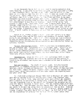 carbon levels were almost identical in milfoil taken from fresh waters as milfoil
taken from brackish waters. Potassium and sodium were concentrated in plants
taken from fresh water, but not in plants from brackish waters. The magnesium
ion increased in the plant as it increased in the water.
In a New Jersey study using plastic ponds and pond water, Ryan et al.
(1972) investigated the effects of fertilization on milfoil, El odea canadensis
and Potamogeton pulcher. The addition of NH^, N03, phosphorus and potassium
added nothing to plant growth the first year. In the second year, £_. pulcher
benefited, but milfoil and El odea grew better in a control environment, possibly
due to no competition from algae. Mulligan et al. (1976) experimented with
nitrogen and phosphorus fertilization on Elodea, milfoil (Myriophyllum spicatum
var. exalbescens), Cfiratophvllum demersum, Potamoqeton crispus and algae in 0.004
ha experimental ponds at Cornell, New York. High fertilization tended to elimin-
ate benthic plant populations and decrease the standing crop of phytoplankton.
Elodea grew in the high nutrient levels, but Ceratophyllum and Myriophyllum were
eliminated. Amonium nitrate and triple super phosphate were used in weekly
applications. Low fertilization rates were 0.05 mg nitrogen/1 and 0.005 phos-
phorus/1; high rates were 100 times the low amounts.
Susceptibility and Control. Due to extensive research initiated to deter-
mine effective methods of control for Myriophyllum spicatum, a strong data base
is available concerning elements,compounds and organisms that negatively impact
milfoil. Natural physical controls such as sedimentation, light, turbidity and
salinity have been discussed previously. Some are quite effective. For instance.
in North Carolina at Pea Island Refuge, just south of Currituck Sound, milfoil
beds were decimated by salt water intrusion in 1962 and by 1967 had not regained
problem status (Crowell et al. 1967).
Bio-controls may cause reduction of milfoil beds also. In 1963, when mil-
foil began to disappear in many areas, some milfoil beds in the Potomac River
were so smothered by blankets of diatomaceous algal growth, that milfoil photo-
synthesis would have to have been highly reduced, if even possible. Other plant
species associated with milfoil were similarly affected, (e.g., Potamogeton
perfoliatus) (Rawls 1964; Steenis and King 1964). A minor controlling influence
might have been barnacles which set on milfoil stems, virtually weighting them
to the bottom, or furnishing resistance to mechanical actions of tides and winds
until the stems became broken. However, since only a node is required to begin
a new plant, thinning of milfoil in such a fashion would be strictly localized
and distribution possibly even enhanced.
Boyer (1960), while experimenting upon milfoil in tubs, found that after
25 days such an intense diatom bloom developed that milfoil growth was inhibited.
Boylen and Brock (1974) identified the diatom Cymbella as epiphytic on stems
and leaves of milfoil decaying under ice in Lake Wingra, Wisconsin. They also
found a heavy epiphytic mat of Oedogonium sp. on milfoil from June to September.
Sparrow (1974) reported a species of the fungus Physoderma found on M_. spicatum
in Squaw Lake, Michigan in 1972.
The Agricultural Research Service through Public Law 480 has sponsored
research on bio-control by insects on plant hosts. Larvae of the moth,
Farponyx stratiotata and the weevil (Litodactylus leucogaster) prefer to feed on
22
image:
carbon levels were almost identical in milfoil taken from fresh waters as milfoil
taken from brackish waters. Potassium and sodium were concentrated in plants
taken from fresh water, but not in plants from brackish waters. The magnesium
ion increased in the plant as it increased in the water.
In a New Jersey study using plastic ponds and pond water, Ryan et al.
(1972) investigated the effects of fertilization on milfoil, El odea canadensis
and Potamogeton pulcher. The addition of NH^, N03, phosphorus and potassium
added nothing to plant growth the first year. In the second year, £_. pulcher
benefited, but milfoil and El odea grew better in a control environment, possibly
due to no competition from algae. Mulligan et al. (1976) experimented with
nitrogen and phosphorus fertilization on Elodea, milfoil (Myriophyllum spicatum
var. exalbescens), Cfiratophvllum demersum, Potamoqeton crispus and algae in 0.004
ha experimental ponds at Cornell, New York. High fertilization tended to elimin-
ate benthic plant populations and decrease the standing crop of phytoplankton.
Elodea grew in the high nutrient levels, but Ceratophyllum and Myriophyllum were
eliminated. Amonium nitrate and triple super phosphate were used in weekly
applications. Low fertilization rates were 0.05 mg nitrogen/1 and 0.005 phos-
phorus/1; high rates were 100 times the low amounts.
Susceptibility and Control. Due to extensive research initiated to deter-
mine effective methods of control for Myriophyllum spicatum, a strong data base
is available concerning elements,compounds and organisms that negatively impact
milfoil. Natural physical controls such as sedimentation, light, turbidity and
salinity have been discussed previously. Some are quite effective. For instance.
in North Carolina at Pea Island Refuge, just south of Currituck Sound, milfoil
beds were decimated by salt water intrusion in 1962 and by 1967 had not regained
problem status (Crowell et al. 1967).
Bio-controls may cause reduction of milfoil beds also. In 1963, when mil-
foil began to disappear in many areas, some milfoil beds in the Potomac River
were so smothered by blankets of diatomaceous algal growth, that milfoil photo-
synthesis would have to have been highly reduced, if even possible. Other plant
species associated with milfoil were similarly affected, (e.g., Potamogeton
perfoliatus) (Rawls 1964; Steenis and King 1964). A minor controlling influence
might have been barnacles which set on milfoil stems, virtually weighting them
to the bottom, or furnishing resistance to mechanical actions of tides and winds
until the stems became broken. However, since only a node is required to begin
a new plant, thinning of milfoil in such a fashion would be strictly localized
and distribution possibly even enhanced.
Boyer (1960), while experimenting upon milfoil in tubs, found that after
25 days such an intense diatom bloom developed that milfoil growth was inhibited.
Boylen and Brock (1974) identified the diatom Cymbella as epiphytic on stems
and leaves of milfoil decaying under ice in Lake Wingra, Wisconsin. They also
found a heavy epiphytic mat of Oedogonium sp. on milfoil from June to September.
Sparrow (1974) reported a species of the fungus Physoderma found on M_. spicatum
in Squaw Lake, Michigan in 1972.
The Agricultural Research Service through Public Law 480 has sponsored
research on bio-control by insects on plant hosts. Larvae of the moth,
Farponyx stratiotata and the weevil (Litodactylus leucogaster) prefer to feed on
22
image:
 milfoil. Another moth species, P_. allionalis, in Florida seems to have similar
habits, but further study is needed (Sailer 1972).
Pumpkinseed (Lepomis gibbosus) was seen (Rawls, personal observation) in
shallow shoreline waters uprooting milfoil by nosing and finning it out of the
substrate until an area large enough to accommodate their nest had been cleared.
When many nests occupied a small area, the small depressions were noticeable in
an otherwise unbroken band of milfoil. Carp, noted for rooting activities and
creation of turbid conditions, can clear an area of milfoil. But by fragmenta-
tion, both carp and pumpkinseed can indirectly aid in milfoil distribution
Steenis and King 1964). Rawls et aT. (1975) gave examples of carp destructive-
ness. Almost 5,000 ha of aquatics were eliminated by carp in the late 1950s on
-on the Susquehanna Flats. In Marshall Creek, off Nomini Creek, a Virginia tri-
butary to the lower Potomac River, a surface mat of milfoil was eradicated by
carp in the last two weeks of May, 1968.
Much research has been conducted on a possible disease control of milfoil.
One of the earliest observations that subsequently led to studies of the "Lake
Venice" disease of Eurasian watermilfoil was made by the late Harold Elser
(Haven and Wass 1963). Elser watched the reduction of milfoil in Lake Venice,
Maryland, during the summer of 1962, and suggested a natural control might be
operating. Elser (1966) said that there might actually be two diseases involved
but since the phenomena affecting the plants were not definitely known to be
diseases, perhaps "valetudinous plants" would be a better word than disease.
The Lake Venice disease had reduced the plant cover from 100 percent to 20 per-
cent by 1963, and to 10 percent by 1964.
The chief characteristic of the disease was a heavy overgrowth of diatoms,
epiphytic algae and various sessile protozoans. These organisms became so
thick that along with the silt they collected, the leaflets became entirely ob-
scured. Elser did not know whether the overgrowth was the disease or the symptom.
By 1964, the so-called Lake Venice disease was seen almost everywhere in the Bay,
usually affecting large areas.
The second disease was first noticed by Maryland biologists Vernon Stotts
and Guy Lerner in the Northeast River, tributary to the northeast corner of the
Susquehanna Flats at the head of the Chesapeake Bay. The condition was charac-
terized by a stiffening of the stem and leaves. As the disease advanced, the
leaves fell off, leaving stiff bare stems which stood out of the water at low
tide. However, the roots apparently were not affected because new growth
started even before all the dead stems were gone. In late June of 1964, the
extensive beds of milfoil in the upper western shore Bay tributaries (Seneca,
Salt Peter and Dundee Creeks) had all but disappeared, but by the first of
August, new growth again had reached the surface. By 1964, the two diseases
were so widespread that it was difficult to find four tons of healthy milfoil
for experiments.
The Department of Chesapeake Bay Affairs, as reported by Johnson (1966),
estimated that by 1966 the total milfoil remaining in the Bay was less than 15
percent of the 40,500 ha estimated to be present in 1963, presumably because of
the diseases. Elser was quoted as having said, "However, during the last week
of July many beds of milfoil suddenly showed a very rapid growth of new stems.
23
image:
milfoil. Another moth species, P_. allionalis, in Florida seems to have similar
habits, but further study is needed (Sailer 1972).
Pumpkinseed (Lepomis gibbosus) was seen (Rawls, personal observation) in
shallow shoreline waters uprooting milfoil by nosing and finning it out of the
substrate until an area large enough to accommodate their nest had been cleared.
When many nests occupied a small area, the small depressions were noticeable in
an otherwise unbroken band of milfoil. Carp, noted for rooting activities and
creation of turbid conditions, can clear an area of milfoil. But by fragmenta-
tion, both carp and pumpkinseed can indirectly aid in milfoil distribution
Steenis and King 1964). Rawls et aT. (1975) gave examples of carp destructive-
ness. Almost 5,000 ha of aquatics were eliminated by carp in the late 1950s on
-on the Susquehanna Flats. In Marshall Creek, off Nomini Creek, a Virginia tri-
butary to the lower Potomac River, a surface mat of milfoil was eradicated by
carp in the last two weeks of May, 1968.
Much research has been conducted on a possible disease control of milfoil.
One of the earliest observations that subsequently led to studies of the "Lake
Venice" disease of Eurasian watermilfoil was made by the late Harold Elser
(Haven and Wass 1963). Elser watched the reduction of milfoil in Lake Venice,
Maryland, during the summer of 1962, and suggested a natural control might be
operating. Elser (1966) said that there might actually be two diseases involved
but since the phenomena affecting the plants were not definitely known to be
diseases, perhaps "valetudinous plants" would be a better word than disease.
The Lake Venice disease had reduced the plant cover from 100 percent to 20 per-
cent by 1963, and to 10 percent by 1964.
The chief characteristic of the disease was a heavy overgrowth of diatoms,
epiphytic algae and various sessile protozoans. These organisms became so
thick that along with the silt they collected, the leaflets became entirely ob-
scured. Elser did not know whether the overgrowth was the disease or the symptom.
By 1964, the so-called Lake Venice disease was seen almost everywhere in the Bay,
usually affecting large areas.
The second disease was first noticed by Maryland biologists Vernon Stotts
and Guy Lerner in the Northeast River, tributary to the northeast corner of the
Susquehanna Flats at the head of the Chesapeake Bay. The condition was charac-
terized by a stiffening of the stem and leaves. As the disease advanced, the
leaves fell off, leaving stiff bare stems which stood out of the water at low
tide. However, the roots apparently were not affected because new growth
started even before all the dead stems were gone. In late June of 1964, the
extensive beds of milfoil in the upper western shore Bay tributaries (Seneca,
Salt Peter and Dundee Creeks) had all but disappeared, but by the first of
August, new growth again had reached the surface. By 1964, the two diseases
were so widespread that it was difficult to find four tons of healthy milfoil
for experiments.
The Department of Chesapeake Bay Affairs, as reported by Johnson (1966),
estimated that by 1966 the total milfoil remaining in the Bay was less than 15
percent of the 40,500 ha estimated to be present in 1963, presumably because of
the diseases. Elser was quoted as having said, "However, during the last week
of July many beds of milfoil suddenly showed a very rapid growth of new stems.
23
image:
 This new growth flowered profusely, a phenomenon which had not been observed
since 1964. The new, lush growth of milfoil remained healthy for about two
weeks when definite symptoms of the disease again appeared. By the middle of
August, the plants again were seriously infected and it appears that beds will
be further diminished."
Elser (1967) stated that by 1965, only 5 percent of the original milfoil
acreage remained in Lake Venice. There was a definite lack of flowering on
diseased specimens, but in July, 1966, with the explosive growth from old stems
(up to 10 cm per day), flowering began immediately.
Bayley et al. (1968) believed pathologic conditions were responsible for
the decline of milfoil. Northeast disease symptoms were transmitted in the
laboratory by a bacteriologically sterile filtrate passed through a 0.2 micron
filter. This could indicate a virus, vi-us-like particle or a toxin as the
etiologic agent. Gram-negative bacilli tained from diseased milfoil probably
represented a secondary infection. Because diseased milfoil in some Bay areas
showed a resurgency of growth in 1967, and successfully flowered, it was thought
possibly to indicate development of genetic resistance to the pathogen, or a
natural cyclic pattern with reduced pathogen virulence.
Southwick (1967-1969) detailed in quarterly progress reports studies of
the Northeast disease of milfoil. In 1968, infectivity of an active filtrate
from diseased milfoil was significantly reduced by heating to 70 C for 30
minutes. This was considered as evidence of virus. Electron microscopy of a
filtrate from diseased plants revealed virus particles 80 millimicrons in length
which resembled the potato yellow dwarf virus in morphology, though smaller. In
1969, Southwick (1967-1969) was unable to detect the milfoil virus by physical
tests on frozen preparations of diseased milfoil. This indicated an agent un-
stable to freezing and storage and not easily characterized by standard viro-
logical techniques. In a later 1969 progress report, Southwick was unable to
isolate the virus and demonstrate infectivity as in 1967 and 1968. He believed
the main wave of the virus had passed but the symptoms persisted. He was unable
to infect milfoil with other common plant viruses. In the last progress report
of 1969, Southwick wrote that milfoil had disappeared from the three study areas,
presumably the Back, Middle and Rhode Rivers. The complete loss was attributed
to diseased conditions in September. He reported that milfoil had continued to
decline the last four years in the'Middle and Rhode Rivers and that summer growth
was not persistent.
Steenis (1970) reported that no virus-type disease factors had been noted
in the Currituck Sound area, that attempts to introduce the disease into TVA
lakes were unsuccessful and that symptoms had been noted in the Chassahowitska
area in Florida, but not in the adjoining Homossassa and Crystal Bay localities.
Attempts by Bayley and Weldon to introduce the disease into Crystal River also
failed. Steenis (1970) pointed out that the disease factors accentuated vulner-
ability to adverse environmental conditions.
Bean et al. (1973) performed a laboratory study on Lake Venice disease.
They were not able to produce diseased plants by direct innoculation of healthy
plants or by growing diseased and healthy plants together. However, plants
under low light intensity innoculated with extracts of diseased tissues produced
24
image:
This new growth flowered profusely, a phenomenon which had not been observed
since 1964. The new, lush growth of milfoil remained healthy for about two
weeks when definite symptoms of the disease again appeared. By the middle of
August, the plants again were seriously infected and it appears that beds will
be further diminished."
Elser (1967) stated that by 1965, only 5 percent of the original milfoil
acreage remained in Lake Venice. There was a definite lack of flowering on
diseased specimens, but in July, 1966, with the explosive growth from old stems
(up to 10 cm per day), flowering began immediately.
Bayley et al. (1968) believed pathologic conditions were responsible for
the decline of milfoil. Northeast disease symptoms were transmitted in the
laboratory by a bacteriologically sterile filtrate passed through a 0.2 micron
filter. This could indicate a virus, vi-us-like particle or a toxin as the
etiologic agent. Gram-negative bacilli tained from diseased milfoil probably
represented a secondary infection. Because diseased milfoil in some Bay areas
showed a resurgency of growth in 1967, and successfully flowered, it was thought
possibly to indicate development of genetic resistance to the pathogen, or a
natural cyclic pattern with reduced pathogen virulence.
Southwick (1967-1969) detailed in quarterly progress reports studies of
the Northeast disease of milfoil. In 1968, infectivity of an active filtrate
from diseased milfoil was significantly reduced by heating to 70 C for 30
minutes. This was considered as evidence of virus. Electron microscopy of a
filtrate from diseased plants revealed virus particles 80 millimicrons in length
which resembled the potato yellow dwarf virus in morphology, though smaller. In
1969, Southwick (1967-1969) was unable to detect the milfoil virus by physical
tests on frozen preparations of diseased milfoil. This indicated an agent un-
stable to freezing and storage and not easily characterized by standard viro-
logical techniques. In a later 1969 progress report, Southwick was unable to
isolate the virus and demonstrate infectivity as in 1967 and 1968. He believed
the main wave of the virus had passed but the symptoms persisted. He was unable
to infect milfoil with other common plant viruses. In the last progress report
of 1969, Southwick wrote that milfoil had disappeared from the three study areas,
presumably the Back, Middle and Rhode Rivers. The complete loss was attributed
to diseased conditions in September. He reported that milfoil had continued to
decline the last four years in the'Middle and Rhode Rivers and that summer growth
was not persistent.
Steenis (1970) reported that no virus-type disease factors had been noted
in the Currituck Sound area, that attempts to introduce the disease into TVA
lakes were unsuccessful and that symptoms had been noted in the Chassahowitska
area in Florida, but not in the adjoining Homossassa and Crystal Bay localities.
Attempts by Bayley and Weldon to introduce the disease into Crystal River also
failed. Steenis (1970) pointed out that the disease factors accentuated vulner-
ability to adverse environmental conditions.
Bean et al. (1973) performed a laboratory study on Lake Venice disease.
They were not able to produce diseased plants by direct innoculation of healthy
plants or by growing diseased and healthy plants together. However, plants
under low light intensity innoculated with extracts of diseased tissues produced
24
image:
 symptoms resembling Lake Venice dise<r-::
under stress conditions and to increase \-' .
organisms.
A natural or biological control o;" a '•• .
duction of herbicides into waters which fr •
undesirable pollutants. Usually bio-con'n
ately available, so often the urgent nox"! '
tion requires the careful and immediate- ••-•
knowledge of what effects such an herbieH
general environmental quality surround'-v; r
Steenis (1966) referred to some nr in-
effectiveness of a herbicide. Laboratov1'
is requisite, but one is not necessari; • * • :<
herbicide that is effective on one pUnt
certain time and in a particular geojrip''"
physical and biological character]':;, ic, ;n
away where an application is made within .n • '. ""
and where environmental parameters appea-
Jersey, milfoil's vulnerable period to !Vl ; . M.-
in the Chesapeake Bay, the vulnerable peri;.: .«:ie
herbicide extends from the last 10 days ^
Apparently, anthesis and density of the r,>': •---.>-•
logical difference.
Sodium arsenite at one time was Vfide'y • •• • " r-t.ion.
In an Iowa lake, Myriophyllum s pi catnip ar/ii •••• • • .
treated from the air and by boat with t.hi? .;-'-: • -• -f ; r,o 5
ppm. Fishes were not adversely affe:f,t-I ••••, . ^ >:
and cray fish were killed (Rose 1955),
Through the years other chemical', ii.v,- '..<,
(1975) used glyphosphate at up to 5,000 p;vi •-. :• •
ineffective in preventing root regrowth. r- ; '-.
2,4-D, Fenac and silvex in weighted emulsioi'.c. - •' -•: . ••- ;
learned that control was hampered and co»ip- '• r •
(Springer and Stewart 1959). Sprinqer ;_;r .->! '••• " • .--j.-'ular
formulations of ^,4-D esters at 2? t'i "1 '-•• ;• ^-' -"lat
2,4-D was less expensive and more speclt; >•'*,- -T-v , -,\-
Steenis and Stotts (1961) found that of !6 O^-'M-. ; • - • -or^en-
trations, 2,4-D as noted above was nior',' ^'• . - • •'.:••;• • be
applied when the tide was ebbing or ne^r " :'•.•••;• . ; • ;ai,hed
the surface and the water temperature v;ar ..•: ^ ' r ' Uq65)
stated that diquat was picked up more rapid'- ..-. •- ..-•* h"=;per-
sal was obtained with it, but that itseffe--'; " -, < ;-, ;o.is
factors such as roiled water and algal -did r,r>\
Beaven (1962) wrote that the most con'• > ; •. u i
tained with esters of 2,4-D (butoxyethano'' , '<- •"• : , :- -j---! ' •• to
butyl ether). Dosage rates at 2? kq/hn 3.0 •• •>-• •'--•*,
and when water movement was limited, the amirv.-1 * ' •• ,.-2.
gave similar results. Herbicides were iiiip'-:'. • ,>
c :~i
image:
symptoms resembling Lake Venice dise<r-::
under stress conditions and to increase \-' .
organisms.
A natural or biological control o;" a '•• .
duction of herbicides into waters which fr •
undesirable pollutants. Usually bio-con'n
ately available, so often the urgent nox"! '
tion requires the careful and immediate- ••-•
knowledge of what effects such an herbieH
general environmental quality surround'-v; r
Steenis (1966) referred to some nr in-
effectiveness of a herbicide. Laboratov1'
is requisite, but one is not necessari; • * • :<
herbicide that is effective on one pUnt
certain time and in a particular geojrip''"
physical and biological character]':;, ic, ;n
away where an application is made within .n • '. ""
and where environmental parameters appea-
Jersey, milfoil's vulnerable period to !Vl ; . M.-
in the Chesapeake Bay, the vulnerable peri;.: .«:ie
herbicide extends from the last 10 days ^
Apparently, anthesis and density of the r,>': •---.>-•
logical difference.
Sodium arsenite at one time was Vfide'y • •• • " r-t.ion.
In an Iowa lake, Myriophyllum s pi catnip ar/ii •••• • • .
treated from the air and by boat with t.hi? .;-'-: • -• -f ; r,o 5
ppm. Fishes were not adversely affe:f,t-I ••••, . ^ >:
and cray fish were killed (Rose 1955),
Through the years other chemical', ii.v,- '..<,
(1975) used glyphosphate at up to 5,000 p;vi •-. :• •
ineffective in preventing root regrowth. r- ; '-.
2,4-D, Fenac and silvex in weighted emulsioi'.c. - •' -•: . ••- ;
learned that control was hampered and co»ip- '• r •
(Springer and Stewart 1959). Sprinqer ;_;r .->! '••• " • .--j.-'ular
formulations of ^,4-D esters at 2? t'i "1 '-•• ;• ^-' -"lat
2,4-D was less expensive and more speclt; >•'*,- -T-v , -,\-
Steenis and Stotts (1961) found that of !6 O^-'M-. ; • - • -or^en-
trations, 2,4-D as noted above was nior',' ^'• . - • •'.:••;• • be
applied when the tide was ebbing or ne^r " :'•.•••;• . ; • ;ai,hed
the surface and the water temperature v;ar ..•: ^ ' r ' Uq65)
stated that diquat was picked up more rapid'- ..-. •- ..-•* h"=;per-
sal was obtained with it, but that itseffe--'; " -, < ;-, ;o.is
factors such as roiled water and algal -did r,r>\
Beaven (1962) wrote that the most con'• > ; •. u i
tained with esters of 2,4-D (butoxyethano'' , '<- •"• : , :- -j---! ' •• to
butyl ether). Dosage rates at 2? kq/hn 3.0 •• •>-• •'--•*,
and when water movement was limited, the amirv.-1 * ' •• ,.-2.
gave similar results. Herbicides were iiiip'-:'. • ,>
c :~i
image:
 attaclay granules and dispersed by an air blower through a hose mounted on the
bow of an outboard motor boat.
Stanley (1974) found in a laboratory study that the effectiveness of 2,-
4-D was twice as great on milfoil growing in soil than on milfoil growing in
sand. Calcium chloride added to sand cultures caused a comparable or greater
increase in 2,4-D effectiveness than sand cultures without calcium chloride.
In TVA field treatments there was up to 48 percent difference in effectiveness
between areas that had the highest natural calcium content and the lowest.
In laboratory experiments, Stanley (1974) investigated the synergistic
effects of combining 2,4-D with other compounds. He found that control effec-
tiveness increased with HgCl2, A1C13, NaCl, NaAs02 and CuSO^. Nad as
a synergist, however, required concentrations so high that it was economically
and environmentally unfeasible. Stanley felt that this high concentration
demand might account for the erratic results in field tests of 2,4-D on milfoil
in estuaries subject to salinity fluctuations.
Controlling milfoil by shutting off light from the plant has been studied.
Smith (1962), in TVA lakes, experimented with black polyethylene covers held
in place over milfoil beds with anchors and floats. In 72 days, this complete
shading killed the plants, while a 21 day period did not (Beaven 1962; Smith
1962). Elser (1967) stated that a black aniline dye had been successfully used
in Arizona in 1947 to shade out plants. It was quite successful, but required
a year to produce results. In 1965 to 1966, experimental use was made of black
plastic anchored and weighted to the bottom or floated over the top of milfoil
beds in the South and Sassafras Rivers. From these experiments, Elser (1967)
concluded that black plastic floated on the surface for a two-week period early
in June would give weed control for the entire summer.
Mechanical control (underwater cutting, mowing, scraping, dragging, water-
jetting with numerous variations and combinations) has also been used in milfoil
eradication attempts. Springer (1959) mentioned that cutting about 15 cm above
the bottom with a small, horizontally-mounted buzz saw made possible the tem-
porary clearance of about 0.5 ha day at a daily cost of $40 (1959 figures).
Revegetation of the cut area occurred during the same or following season but
the cut portions created new infestations. Elser (1966, 1967) described dif-
ferent devices used for cutting and/or removing aquatic weeds: hydraulic jets;
a 15 m steel ribbon with saw teeth on both sides and wooden handles on the ends;
and a V-shaped blade dragged along the bottom. He also mentioned that the
Department of Chesapeake Bay Affairs owned a large harvester which, though it
did a good job, would have taken 37 years to get around once to all the Bay's
weed beds, even if the machine would work all year-round. Mowing, at best,
Elser concluded, was a temporary measure. Rawls (1964, 1975) concluded that
mowing alone was effective only for a season and had to be repeated monthly,
depending on the type of activity necessitating the mowing. Cutting followed
by 2,4-D application at usual rates extended milfoil's vulnerable period beyond
anthesis, but the control effects were scarcely noticeable the following season.
Mowing seemed to be practical only for small areas such as private boat docks,
small marinas, opening short channels to open water, etc.
26
image:
attaclay granules and dispersed by an air blower through a hose mounted on the
bow of an outboard motor boat.
Stanley (1974) found in a laboratory study that the effectiveness of 2,-
4-D was twice as great on milfoil growing in soil than on milfoil growing in
sand. Calcium chloride added to sand cultures caused a comparable or greater
increase in 2,4-D effectiveness than sand cultures without calcium chloride.
In TVA field treatments there was up to 48 percent difference in effectiveness
between areas that had the highest natural calcium content and the lowest.
In laboratory experiments, Stanley (1974) investigated the synergistic
effects of combining 2,4-D with other compounds. He found that control effec-
tiveness increased with HgCl2, A1C13, NaCl, NaAs02 and CuSO^. Nad as
a synergist, however, required concentrations so high that it was economically
and environmentally unfeasible. Stanley felt that this high concentration
demand might account for the erratic results in field tests of 2,4-D on milfoil
in estuaries subject to salinity fluctuations.
Controlling milfoil by shutting off light from the plant has been studied.
Smith (1962), in TVA lakes, experimented with black polyethylene covers held
in place over milfoil beds with anchors and floats. In 72 days, this complete
shading killed the plants, while a 21 day period did not (Beaven 1962; Smith
1962). Elser (1967) stated that a black aniline dye had been successfully used
in Arizona in 1947 to shade out plants. It was quite successful, but required
a year to produce results. In 1965 to 1966, experimental use was made of black
plastic anchored and weighted to the bottom or floated over the top of milfoil
beds in the South and Sassafras Rivers. From these experiments, Elser (1967)
concluded that black plastic floated on the surface for a two-week period early
in June would give weed control for the entire summer.
Mechanical control (underwater cutting, mowing, scraping, dragging, water-
jetting with numerous variations and combinations) has also been used in milfoil
eradication attempts. Springer (1959) mentioned that cutting about 15 cm above
the bottom with a small, horizontally-mounted buzz saw made possible the tem-
porary clearance of about 0.5 ha day at a daily cost of $40 (1959 figures).
Revegetation of the cut area occurred during the same or following season but
the cut portions created new infestations. Elser (1966, 1967) described dif-
ferent devices used for cutting and/or removing aquatic weeds: hydraulic jets;
a 15 m steel ribbon with saw teeth on both sides and wooden handles on the ends;
and a V-shaped blade dragged along the bottom. He also mentioned that the
Department of Chesapeake Bay Affairs owned a large harvester which, though it
did a good job, would have taken 37 years to get around once to all the Bay's
weed beds, even if the machine would work all year-round. Mowing, at best,
Elser concluded, was a temporary measure. Rawls (1964, 1975) concluded that
mowing alone was effective only for a season and had to be repeated monthly,
depending on the type of activity necessitating the mowing. Cutting followed
by 2,4-D application at usual rates extended milfoil's vulnerable period beyond
anthesis, but the control effects were scarcely noticeable the following season.
Mowing seemed to be practical only for small areas such as private boat docks,
small marinas, opening short channels to open water, etc.
26
image:
 As previously pointed out, salt water intrusion decimated Eurasian water-
milfoil in the lower Potomac River in 1933 and at Pea Island National Wildlife
Refuge in 1962. Knowles (1976) developed two models evaluating control through
salinity manipulation in Currituck Sound, Economically, neither the pumping in
of salt water or the opening of an inlet to the sea seemed feasible. Also, if
salinity were to be raised, other fresh water macrophytes would probably be ex-
cluded.
A further control method that has met with success in TVA lakes is water
level manipulation along with herbicide application. However, conditions with-
in the Chesapeake Bay estuary preclude the use of such measures.
Productivity
Productivity of Myriophyllum in the natural environment is influenced by
a host of environmental factors. Inclusive are carbon sources and concentra-
tions, light, temperature and salinity. Variations in these factors may affect
productivity alone or variations in two or more factors may produce synergistic
or antagonistic interactions.
Myriophyl1 urnis able to utilize the bicarbonate ion as a carbon source
(Anderson 1964; Hutchinson 1970, cited in Nichols 1975; Van et al. 1976) though
free C02 is the preferred form (Van et al. 1976; Steemann Nielson 1951). Mil-
foil can also utilize half-bound C02 (Patten 1956). Carbon sources are absorb-
ed by both the upper and lower leaf surfaces. The absorption and subsequent
translocatiqn is linearly dependent on the ion concentration up to a concentra-
tion of 10~°M CO?(HC03~) /I under optimum light conditions. There is a decrease
in HC03" adsorption when Myriophyllum is switched from a balanced salt solution
to a pure solution of KHC03, NaHC03 or Ca(HC03)2 with the same HC03~ concentra-
tion. Photosynthesis rates respond rapidly to changes in aqueous concentrations
of carbon with decreasing photosynthesis as carbon levels decrease (McCraken
et al. 1975).
Hydrogen ion concentration indirectly affects photosynthesis by affecting
the carbon concentration. Milfoil photosynthesis, when taken from pH 3.1 to
9.3, is unduly affected by the reduction in free C02 (Van et al. 1976); however,
Shiyan and Merezhko (1972) found the efficiency of milfoil to be 10 times higher
in alkaline solutions than in acid conditions provided in two had equal C02 con-
centrations.
Titus et al. (1975) pointed out that milfoil has the potential of becoming
a plant nuisance in thermally enriched environments, probably due to high optimum
temperatures required for milfoil photosynthesis.
Several authors have reported on the effects of light on photosynthesis.
Steemann Nielson (1951) in a laboratory study with milfoil grown in optimum light
and in optimum HC03~ concentration showed that photosynthesis was not limited
by a photochemical reaction. In Lake Wingra, Wisconsin, Adams et al. (1974)
found that at a depth of 2.4 m, 56 percent of the photosynthetic activity
occurred within 1.0 m of the surface in May. In August, 57 percent occurred
within only 20 cm of the surface. They concluded that light and depth distri-
bution of photosynthetic tissue was most important in causing variation in
27
image:
As previously pointed out, salt water intrusion decimated Eurasian water-
milfoil in the lower Potomac River in 1933 and at Pea Island National Wildlife
Refuge in 1962. Knowles (1976) developed two models evaluating control through
salinity manipulation in Currituck Sound, Economically, neither the pumping in
of salt water or the opening of an inlet to the sea seemed feasible. Also, if
salinity were to be raised, other fresh water macrophytes would probably be ex-
cluded.
A further control method that has met with success in TVA lakes is water
level manipulation along with herbicide application. However, conditions with-
in the Chesapeake Bay estuary preclude the use of such measures.
Productivity
Productivity of Myriophyllum in the natural environment is influenced by
a host of environmental factors. Inclusive are carbon sources and concentra-
tions, light, temperature and salinity. Variations in these factors may affect
productivity alone or variations in two or more factors may produce synergistic
or antagonistic interactions.
Myriophyl1 urnis able to utilize the bicarbonate ion as a carbon source
(Anderson 1964; Hutchinson 1970, cited in Nichols 1975; Van et al. 1976) though
free C02 is the preferred form (Van et al. 1976; Steemann Nielson 1951). Mil-
foil can also utilize half-bound C02 (Patten 1956). Carbon sources are absorb-
ed by both the upper and lower leaf surfaces. The absorption and subsequent
translocatiqn is linearly dependent on the ion concentration up to a concentra-
tion of 10~°M CO?(HC03~) /I under optimum light conditions. There is a decrease
in HC03" adsorption when Myriophyllum is switched from a balanced salt solution
to a pure solution of KHC03, NaHC03 or Ca(HC03)2 with the same HC03~ concentra-
tion. Photosynthesis rates respond rapidly to changes in aqueous concentrations
of carbon with decreasing photosynthesis as carbon levels decrease (McCraken
et al. 1975).
Hydrogen ion concentration indirectly affects photosynthesis by affecting
the carbon concentration. Milfoil photosynthesis, when taken from pH 3.1 to
9.3, is unduly affected by the reduction in free C02 (Van et al. 1976); however,
Shiyan and Merezhko (1972) found the efficiency of milfoil to be 10 times higher
in alkaline solutions than in acid conditions provided in two had equal C02 con-
centrations.
Titus et al. (1975) pointed out that milfoil has the potential of becoming
a plant nuisance in thermally enriched environments, probably due to high optimum
temperatures required for milfoil photosynthesis.
Several authors have reported on the effects of light on photosynthesis.
Steemann Nielson (1951) in a laboratory study with milfoil grown in optimum light
and in optimum HC03~ concentration showed that photosynthesis was not limited
by a photochemical reaction. In Lake Wingra, Wisconsin, Adams et al. (1974)
found that at a depth of 2.4 m, 56 percent of the photosynthetic activity
occurred within 1.0 m of the surface in May. In August, 57 percent occurred
within only 20 cm of the surface. They concluded that light and depth distri-
bution of photosynthetic tissue was most important in causing variation in
27
image:
 photosynthesis. McCracken et al. (1975) stated that photosynthesis peaked at
mid-day or shortly thereafter.
Photosynthesis, but not respiration, appears to be affected by salinity
although there seems to be a controversy. Without giving quantitative salinity
measurements, Boyer (1960) stated that there was no difference in milfoil res-
piration and photosynthesis in fresh or saline waters. However, in the labora-
tory, McGahee and Davis (1971) demonstrated a depression in photosynthesis
when apical portions of My r i o p hy 11 urn we re taken from lower to higher salinities
and whole plants were killed or stunted at 13 to 14 ppt. Graham and Davis
(1972) found that photosynthesis was inhibited at 32 ppt after 20 hours but
that respiration was unaffected. After 10 days at 16 ppt photosynthesis was
low. At salinities of 4, 8, 16 and 32 ppt, net photosynthesis was found to
decrease with increased salinity in light bottles, but again respiration was
little affected in dark bottles. The effect was found to be reversed if CaCl2
was added to high concentrations (1:22 and 0.1:22 Ca:Na). At lower concentra-
tions (0:22 and 0.01:22 Ca:Na), milfoil cells were observed to disintegrate
and the membranes ruptured (Davis et al. 1974).
McGahee and Davis (1971) studied interactions between light and depth in
regard to photosynthesis of apical portions of Myriophyllum collected in water
0 ppt salinity. Under 20 hours of low light in constant illumination and in
32 ppt, photosynthesis was depressed but neither photosynthesis nor respira-
tion was affected when salinity was lowered. With moderate light in a light/
dark regime of 10 hours/14 hours, photosynthesis was inhibited at 16 ppt and
respiration remained high.
Milfoil grows rapidly. In the Chesapeake Bay, during its mid-summer pro-
duction peak, it can grow 2.5 cm a day after being severed by an underwater
mower (Rawls 1964), or after being cut in other growth periods, as much as
45 cm per month from a new node (Rawls 1975). Smith (1962) found 1 m of
growth in one season from a 7 cm fragment in a TVA lake. In turbid waters
where the lower leaves are sloughed off, the same biomass tends to become con-
centrated in the upper canopy. Loss of lower leaves also occurs in non-turbid
waters of the Chesapeake, and appears to be characteristic of Myriophllum
spicatum particularly in dense beds (Rawls, personal observation).
Adams et al. (1974) determined that the maximum ash-free dry weight of
a standing crop of milfoil (220 g/m2) was about 100 g C/m2. Nicholson and
Post (1975) stated that ash content was required to estimate organic produc-
tion and possible economic uses. Ash content increased with alkalinity in
the Haloragaceae but not in some other aquatic plant families.
Consumer Uti1ization
As with most submersed aquatic vegetation species, Eurasian watermilfoil
provides some or all of the basic life requirements—food, shelter, protection,
nesting and resting—for animals and to a lesser extent, plant species assoc-
iated with it or coming in contact with it.
Many of the minnows and larger fish are known to deposit eggs on sub-
mersed vegetation. When plant species serving this purpose are listed,
28
image:
photosynthesis. McCracken et al. (1975) stated that photosynthesis peaked at
mid-day or shortly thereafter.
Photosynthesis, but not respiration, appears to be affected by salinity
although there seems to be a controversy. Without giving quantitative salinity
measurements, Boyer (1960) stated that there was no difference in milfoil res-
piration and photosynthesis in fresh or saline waters. However, in the labora-
tory, McGahee and Davis (1971) demonstrated a depression in photosynthesis
when apical portions of My r i o p hy 11 urn we re taken from lower to higher salinities
and whole plants were killed or stunted at 13 to 14 ppt. Graham and Davis
(1972) found that photosynthesis was inhibited at 32 ppt after 20 hours but
that respiration was unaffected. After 10 days at 16 ppt photosynthesis was
low. At salinities of 4, 8, 16 and 32 ppt, net photosynthesis was found to
decrease with increased salinity in light bottles, but again respiration was
little affected in dark bottles. The effect was found to be reversed if CaCl2
was added to high concentrations (1:22 and 0.1:22 Ca:Na). At lower concentra-
tions (0:22 and 0.01:22 Ca:Na), milfoil cells were observed to disintegrate
and the membranes ruptured (Davis et al. 1974).
McGahee and Davis (1971) studied interactions between light and depth in
regard to photosynthesis of apical portions of Myriophyllum collected in water
0 ppt salinity. Under 20 hours of low light in constant illumination and in
32 ppt, photosynthesis was depressed but neither photosynthesis nor respira-
tion was affected when salinity was lowered. With moderate light in a light/
dark regime of 10 hours/14 hours, photosynthesis was inhibited at 16 ppt and
respiration remained high.
Milfoil grows rapidly. In the Chesapeake Bay, during its mid-summer pro-
duction peak, it can grow 2.5 cm a day after being severed by an underwater
mower (Rawls 1964), or after being cut in other growth periods, as much as
45 cm per month from a new node (Rawls 1975). Smith (1962) found 1 m of
growth in one season from a 7 cm fragment in a TVA lake. In turbid waters
where the lower leaves are sloughed off, the same biomass tends to become con-
centrated in the upper canopy. Loss of lower leaves also occurs in non-turbid
waters of the Chesapeake, and appears to be characteristic of Myriophllum
spicatum particularly in dense beds (Rawls, personal observation).
Adams et al. (1974) determined that the maximum ash-free dry weight of
a standing crop of milfoil (220 g/m2) was about 100 g C/m2. Nicholson and
Post (1975) stated that ash content was required to estimate organic produc-
tion and possible economic uses. Ash content increased with alkalinity in
the Haloragaceae but not in some other aquatic plant families.
Consumer Uti1ization
As with most submersed aquatic vegetation species, Eurasian watermilfoil
provides some or all of the basic life requirements—food, shelter, protection,
nesting and resting—for animals and to a lesser extent, plant species assoc-
iated with it or coming in contact with it.
Many of the minnows and larger fish are known to deposit eggs on sub-
mersed vegetation. When plant species serving this purpose are listed,
28
image:
 milfoil is frequently among them. Rawls (1975) observed fishermen casting for
largetnouth black bass (Micropterus salmoides) along the edges of experimental
plots cleared of milfoil in Dundee Creek.The fishermen reported excellent
catches as long as plots remained open. Crowell et al. (1967) reported that
in the Currituck Sound-Back Bay area, an increase in sport fishermen catch rates
occurred until milfoil beds became so dense the edge effect was lost.
Patten (1956) stated that waterfowl feed upon milfoil achenes, and from
his literature cited, mentioned that Guppy in 1897 suggested that seed germina-
tion might be increased by passage through the alimentary system of birds.
Patten (1956) concluded that waterfowl were probably the most important disper-
sal agents of fruits to various drainage systems. However in food habit studies
in the Chesapeake Bay (Rawls, in press), most of the milfoil seeds in waterfowl
gizzards were crushed and broken by the powerful grinding action of the gizzard,
unless the seeds were freshly ingested. Patten (1956) suggested that the small,
slime-covered spring buds or turions were able to adhere to waterfowl feet be-
cause of a glucosidic envelope and provided a potential source for milfoil dis-
tribution into new areas.
Springer and Stewart (1959) reported that Coot (Fulica americana), Wigeon
(Anas americana) and probably Gadwall (Anas strepera) have been observed feeding
on milfoil. Crowell et al. (1967) discovered that apparent feeding by water-
fowl on milfoil in the Currituck Sound-Back Bay area was deceiving. Milfoil
was growing in the same type habitat as were preferred plant foods and after
about the third year, as desirable foods were crowded out by milfoil, waterfowl
left and moved to areas where choice foods still existed.
Bayley et al. (in press) observed that waterfowl numbers decreased on the
Susquehanna Flats during the period of greatest milfoil abundance. Martin et al.
(1951) classified milfoil as a low grade duck food. However, though the quantity
of woody seeds eaten was usually small, the nutlets were eaten to a considerable
extent in the prairie lakes of the Dakotas and in adjoining states. Florschutz
(1973) examined the contents of 170 waterfowl digestive tracts collected in the
vicinity of Back Bay and Currituck Sound during hunting seasons from 1968 to
1971. Included were 27 Canada Geese, 6 species of dabbling ducks, and 4 species
of diving ducks, plus 31 Coots. Milfoil was found in 71.8 percent of the birds
and comprised about 33 percent of the total food volume. The highest milfoil
use was noted in Scaups. Rawls (in press) examined 2,747 waterfowl gizzards
taken during hunting seasons in the Chesapeake Bay area during 1959 to 1968.
Represented were 2 species of geese, 6 species of dabblers, 8 species of divers
and 1 species of Merganser. Slightly over 10 percent contained milfoil seed,
stems or leaves. In volume, milfoil averaged 4.2 percent by volume of all foods
eaten, and per individual bird, ranged from zero or trace amounts to 100 percent.
Wigeons used milfoil to the greatest extent (over 21 percent) of all birds ex-
amined.
Milfoil offers attachment sites for organisms which later become food for
higher life forms (Springer 1959; Springer et al. 1961). Patten (1956) found
that milfoil offered support for attached Aufwuchs and detached organisms such
as tychoplankton and that milfoil, because of its finely dissected leaves, could
support more periphyton than most other aquatic phanerogams.
29
image:
milfoil is frequently among them. Rawls (1975) observed fishermen casting for
largetnouth black bass (Micropterus salmoides) along the edges of experimental
plots cleared of milfoil in Dundee Creek.The fishermen reported excellent
catches as long as plots remained open. Crowell et al. (1967) reported that
in the Currituck Sound-Back Bay area, an increase in sport fishermen catch rates
occurred until milfoil beds became so dense the edge effect was lost.
Patten (1956) stated that waterfowl feed upon milfoil achenes, and from
his literature cited, mentioned that Guppy in 1897 suggested that seed germina-
tion might be increased by passage through the alimentary system of birds.
Patten (1956) concluded that waterfowl were probably the most important disper-
sal agents of fruits to various drainage systems. However in food habit studies
in the Chesapeake Bay (Rawls, in press), most of the milfoil seeds in waterfowl
gizzards were crushed and broken by the powerful grinding action of the gizzard,
unless the seeds were freshly ingested. Patten (1956) suggested that the small,
slime-covered spring buds or turions were able to adhere to waterfowl feet be-
cause of a glucosidic envelope and provided a potential source for milfoil dis-
tribution into new areas.
Springer and Stewart (1959) reported that Coot (Fulica americana), Wigeon
(Anas americana) and probably Gadwall (Anas strepera) have been observed feeding
on milfoil. Crowell et al. (1967) discovered that apparent feeding by water-
fowl on milfoil in the Currituck Sound-Back Bay area was deceiving. Milfoil
was growing in the same type habitat as were preferred plant foods and after
about the third year, as desirable foods were crowded out by milfoil, waterfowl
left and moved to areas where choice foods still existed.
Bayley et al. (in press) observed that waterfowl numbers decreased on the
Susquehanna Flats during the period of greatest milfoil abundance. Martin et al.
(1951) classified milfoil as a low grade duck food. However, though the quantity
of woody seeds eaten was usually small, the nutlets were eaten to a considerable
extent in the prairie lakes of the Dakotas and in adjoining states. Florschutz
(1973) examined the contents of 170 waterfowl digestive tracts collected in the
vicinity of Back Bay and Currituck Sound during hunting seasons from 1968 to
1971. Included were 27 Canada Geese, 6 species of dabbling ducks, and 4 species
of diving ducks, plus 31 Coots. Milfoil was found in 71.8 percent of the birds
and comprised about 33 percent of the total food volume. The highest milfoil
use was noted in Scaups. Rawls (in press) examined 2,747 waterfowl gizzards
taken during hunting seasons in the Chesapeake Bay area during 1959 to 1968.
Represented were 2 species of geese, 6 species of dabblers, 8 species of divers
and 1 species of Merganser. Slightly over 10 percent contained milfoil seed,
stems or leaves. In volume, milfoil averaged 4.2 percent by volume of all foods
eaten, and per individual bird, ranged from zero or trace amounts to 100 percent.
Wigeons used milfoil to the greatest extent (over 21 percent) of all birds ex-
amined.
Milfoil offers attachment sites for organisms which later become food for
higher life forms (Springer 1959; Springer et al. 1961). Patten (1956) found
that milfoil offered support for attached Aufwuchs and detached organisms such
as tychoplankton and that milfoil, because of its finely dissected leaves, could
support more periphyton than most other aquatic phanerogams.
29
image:
 Economic Uses and Problems
The redeeming qualities of milfoil are not as noticeable as the problems
it causes. However, Myriophyllum spicatum is not totally devoid of positive
features. Springer (1959) noted that milfoil could occupy sites which other-
wise would be inhabited by objectionable algae. Nichols (1975) found that
milfoil was a good hydrosol stabilizer, and as animal food, had a high xantho-
phyll content and was comparable to alfalfa in protein content. However, Haven
and Wass (1963) noted that milfoil xanthophyll was unstable. Haven and Mass
(1963) reported that the amounts of Ca, K, Na, N, P, and Mg were insufficient
to class milfoil as a good source of nutritive elements.
Elser (1966) reported that the high ash content of milfoil precluded its
use as a chicken food because it gave the birds diarrhea. As cattle food, it
was about as good as high quality hay (about 19 percent protein). Milfoil's
chief drawback was its water content of 90 percent . Elser (1966) added that
one Annapolis high school girl made cookies of milfoil flour and pronounced
them good. Elser (1967) wrote that milfoil's N-P-K value was 3-2-5. This was
better than cow (2-1-1) or sheep (1-1-2) manure (Elser 1965).
However, the story of milfoil is concerned less with pleasure and more
with vexation ranging from mildly annoying to verging on economic disaster.
In order to cope with ramifications of the milfoil explosion, an interagency
cooperative effort of personnel representing Federal, state, private, educa-
tional, commercial and industrial interests plus representatives of the general
public met annually from 1959 through 1964 to discuss any and all aspects of
milfoil infestation not only in Maryland, but in other affected areas. Agencies
and their representatives most active in milfoil investigations in the Chesapeake
Bay area were: U.S. Fish and Wildlife Service, Patuxent Wildlife Research Center
(John Steenis); Maryland Department of Natural Resources Wildlife Administration
(Vernon Stotts); Virginia Institute of Marine Science (Dexter Haven); University
of Maryland, Chesapeake Biological Laboratory (Charles K. Rawls, Gordon Beckett,
Theordore Will and G. Francis Beaven).
By early 1963 (Kelly 1963), milfoil had become such a problem that a noxious
weed bill H.R. 2994 (Morton) was introducted in the House of Representatives.
The bill provided for the control and progressive eradication of certain aquatic
plants in Maryland, Virginia, New Jersey and Tennessee. It was concerned with
Eurasian watermilfoil and involved Federal and state cooperation through the
U.S. Army Corps of Engineers.
The impacts of the milfoil explosion were felt in many areas of the
Chesapeake Bay. Waterfowl distribution was affected because winter feeding
grounds, such as the Susquehanna Flats, seemed to lose their attractiveness to
many species of water birds, among them, Canvasback (Aythya vallisneria), a
threatened species. Springer et al. (1961) identified some of the aquatic plants
favored by waterfowl for food which milfoil chokes out: Potamogeton pectinatus
Vallisneria americana and Ruppia maritima. Steenis and Stotts (1961) noted that
oxygen was reduced under the heavy, surface milfoil blanket.
30
image:
Economic Uses and Problems
The redeeming qualities of milfoil are not as noticeable as the problems
it causes. However, Myriophyllum spicatum is not totally devoid of positive
features. Springer (1959) noted that milfoil could occupy sites which other-
wise would be inhabited by objectionable algae. Nichols (1975) found that
milfoil was a good hydrosol stabilizer, and as animal food, had a high xantho-
phyll content and was comparable to alfalfa in protein content. However, Haven
and Wass (1963) noted that milfoil xanthophyll was unstable. Haven and Mass
(1963) reported that the amounts of Ca, K, Na, N, P, and Mg were insufficient
to class milfoil as a good source of nutritive elements.
Elser (1966) reported that the high ash content of milfoil precluded its
use as a chicken food because it gave the birds diarrhea. As cattle food, it
was about as good as high quality hay (about 19 percent protein). Milfoil's
chief drawback was its water content of 90 percent . Elser (1966) added that
one Annapolis high school girl made cookies of milfoil flour and pronounced
them good. Elser (1967) wrote that milfoil's N-P-K value was 3-2-5. This was
better than cow (2-1-1) or sheep (1-1-2) manure (Elser 1965).
However, the story of milfoil is concerned less with pleasure and more
with vexation ranging from mildly annoying to verging on economic disaster.
In order to cope with ramifications of the milfoil explosion, an interagency
cooperative effort of personnel representing Federal, state, private, educa-
tional, commercial and industrial interests plus representatives of the general
public met annually from 1959 through 1964 to discuss any and all aspects of
milfoil infestation not only in Maryland, but in other affected areas. Agencies
and their representatives most active in milfoil investigations in the Chesapeake
Bay area were: U.S. Fish and Wildlife Service, Patuxent Wildlife Research Center
(John Steenis); Maryland Department of Natural Resources Wildlife Administration
(Vernon Stotts); Virginia Institute of Marine Science (Dexter Haven); University
of Maryland, Chesapeake Biological Laboratory (Charles K. Rawls, Gordon Beckett,
Theordore Will and G. Francis Beaven).
By early 1963 (Kelly 1963), milfoil had become such a problem that a noxious
weed bill H.R. 2994 (Morton) was introducted in the House of Representatives.
The bill provided for the control and progressive eradication of certain aquatic
plants in Maryland, Virginia, New Jersey and Tennessee. It was concerned with
Eurasian watermilfoil and involved Federal and state cooperation through the
U.S. Army Corps of Engineers.
The impacts of the milfoil explosion were felt in many areas of the
Chesapeake Bay. Waterfowl distribution was affected because winter feeding
grounds, such as the Susquehanna Flats, seemed to lose their attractiveness to
many species of water birds, among them, Canvasback (Aythya vallisneria), a
threatened species. Springer et al. (1961) identified some of the aquatic plants
favored by waterfowl for food which milfoil chokes out: Potamogeton pectinatus
Vallisneria americana and Ruppia maritima. Steenis and Stotts (1961) noted that
oxygen was reduced under the heavy, surface milfoil blanket.
30
image:
 Milfoil interferes with oyster (Crassostrea virginica) growth by reducing
water movement and restricting flow of food to oysters. Lack of water move-
ment also permits surface water temperatures to increase to the point they may
have detrimental effects to plants and animals in shallow waters. Anaerobic
conditions arise as a result of decomposing milfoil, and sulphur bacteria then
release hydrogen sulfide, killing the oysters. In addition, dense mats make
harvest almost impossible by dredge and tongs.
Milfoil seriously interferes with angling, with fishing by means of haul
seines or fyke nets and with crabbing by pots, trot lines and scrapers. Milfoil
also restricts navigation for commercial fisheries, curtails pleasure boating,
water skiing, swimming and clogs water intakes in pumps and motors. It con-
tributes to a more rapid build-up of the bottom through deposition of organic
material and facilitation of silting. Milfoil beds appear to provide conditions
suitable for mosquito (Anopheles quadrimaculatus) and possibly certain Culex sp.
Undesirable odors are created by windrows of decomposing vegetation deposited by
wind and tide on shorelines. The possibility exists that milfoil can impart
off-tastes to the water and it may lower nearby real estate values.
ZOSTERA MARINA2
Biology
General Morphology. Zostera marina is one of the few species of aquatic
plants to inhabit the marine environment (Hartog 1970). It is a true flowering
plant belonging to the phylum Spermatophyta and to the class Monocotyledoneae
or plants with embryos with a single cotyledon. It is a member of the pondweed
family, the Potamogetonaceae. The plant is known commonly by many names, the
most widely used being eel grass, but sometimes referred to as grass wrack. The
name Zostera comes from the Greek word Zoster, a belt, in reference to the long,
blade-like leaves of the sea.
Eel grass has a creeping rhizome, 2 to 5 mm thick, with numerous roots and
a leaf at each node. Internodes are 10 to 35 mm long. The tubular, membranous
leaf sheath may be 5 to 20 cm long and is wider than the leaf-blade. The leaf-
blade may be up to 120 cm long and 2 to 12 mm wide with 5 to 11 nerves (Hartog
1970) (see Figure 7).
The leaf-blade of eelgrass displays a variety of morphological forms de-
pending on the depth of the water, salinity, temperature, current regimes and
sedimentological characteristics (sand, mud, related nutrients) (Orth, in press;
Ostenfeld 1905; Butcher 1935; Burkholder and Doheny 1968; Harrison and Mann 1975
Hartog 1970; Setchell 1927, 1929; Phillips and Grant 1965; Phillips 1972; McRoy
1966, 1970ju 1970b_; Philip 1936). In general, eelgrass has usually displayed
the small narrow-leaf form in shallow, more physically exposed, sandy substrates
2Special contribution from Rober Orth, Virginia Institute of Marine Science
31
image:
Milfoil interferes with oyster (Crassostrea virginica) growth by reducing
water movement and restricting flow of food to oysters. Lack of water move-
ment also permits surface water temperatures to increase to the point they may
have detrimental effects to plants and animals in shallow waters. Anaerobic
conditions arise as a result of decomposing milfoil, and sulphur bacteria then
release hydrogen sulfide, killing the oysters. In addition, dense mats make
harvest almost impossible by dredge and tongs.
Milfoil seriously interferes with angling, with fishing by means of haul
seines or fyke nets and with crabbing by pots, trot lines and scrapers. Milfoil
also restricts navigation for commercial fisheries, curtails pleasure boating,
water skiing, swimming and clogs water intakes in pumps and motors. It con-
tributes to a more rapid build-up of the bottom through deposition of organic
material and facilitation of silting. Milfoil beds appear to provide conditions
suitable for mosquito (Anopheles quadrimaculatus) and possibly certain Culex sp.
Undesirable odors are created by windrows of decomposing vegetation deposited by
wind and tide on shorelines. The possibility exists that milfoil can impart
off-tastes to the water and it may lower nearby real estate values.
ZOSTERA MARINA2
Biology
General Morphology. Zostera marina is one of the few species of aquatic
plants to inhabit the marine environment (Hartog 1970). It is a true flowering
plant belonging to the phylum Spermatophyta and to the class Monocotyledoneae
or plants with embryos with a single cotyledon. It is a member of the pondweed
family, the Potamogetonaceae. The plant is known commonly by many names, the
most widely used being eel grass, but sometimes referred to as grass wrack. The
name Zostera comes from the Greek word Zoster, a belt, in reference to the long,
blade-like leaves of the sea.
Eel grass has a creeping rhizome, 2 to 5 mm thick, with numerous roots and
a leaf at each node. Internodes are 10 to 35 mm long. The tubular, membranous
leaf sheath may be 5 to 20 cm long and is wider than the leaf-blade. The leaf-
blade may be up to 120 cm long and 2 to 12 mm wide with 5 to 11 nerves (Hartog
1970) (see Figure 7).
The leaf-blade of eelgrass displays a variety of morphological forms de-
pending on the depth of the water, salinity, temperature, current regimes and
sedimentological characteristics (sand, mud, related nutrients) (Orth, in press;
Ostenfeld 1905; Butcher 1935; Burkholder and Doheny 1968; Harrison and Mann 1975
Hartog 1970; Setchell 1927, 1929; Phillips and Grant 1965; Phillips 1972; McRoy
1966, 1970ju 1970b_; Philip 1936). In general, eelgrass has usually displayed
the small narrow-leaf form in shallow, more physically exposed, sandy substrates
2Special contribution from Rober Orth, Virginia Institute of Marine Science
31
image:
 (copied from Hotchkiss 1967)
Figure 7. Eelgrass (Zostera marina)
32
image:
(copied from Hotchkiss 1967)
Figure 7. Eelgrass (Zostera marina)
32
image:
 while in deeper muddy and/or less exposed areas, the longer, wider form pre-
dominates. These characteristics are typical of the eelgrass found in various
locations in the Chesapeake Bay with one exception. The eelgrass at Tangier
Island is exceedingly lush (turions over 1 m long in water only 0.3 m at MLW)
and may be a response to nutrient addition from the adjacent, low lying, un-
sewered community. Orth (in press) found that the addition of commercial fer-
tilizer increased the growth of eelgrass significantly (both length of turions
and biomass) in a bed on the Eastern Shore of Virginia and suggested that the
growth form may be a function of the amount of nutrients in the sediment. Sedi-
mentary nutrient content may in turn be directly related to sediment type (i.e.
mud or sand).
This difference in growth form has created some taxonomic problems in that
two species of eelgrass have been described, one for each form (Hartog 1970).
However, Phillips (1972, 1974bJ has demonstrated via transplants, that eelgrass
maintains phenotypic plasticity and conforms to the conditions of its environ-
ment. One interesting observation is that of Blackburn (1934) who noted that
after the wasting disease in the 1930s in England the narrow-leaf form returned
in areas where the wide leaf form had previously been found. The drastic change
in sediment type after the disappearance of eelgrass (mud to sand and associated
nutrient changes) may have resulted in the change in form of the grass. Similar
observations have been made in the York River, Virginia, after the disappearance
of eelgrass in this area (Orth, personal observation). The eelgrass inhabiting
these areas, in what were once extensive meadows, is of the short, narrow leafed
variety where, prior to the loss, the long, wide-leaf form was prevalent. The
sediments in this area have been drastically altered after the removal of eel-
grass (Orth 1975a).
Reproduction. Vegetative propagation as in most other aquatic plants occurs
via elongation and growth of the rhizome. Sexual reproduction occurs with the
formation of generative shoots which are erect branches born from the prostrate
perennial rhizome. These shoots are normally terminal on the rhizome (Churchill,
in press; McRoy 1966; Orth, personal observation; Setchell 1929) but may appear
on lateral branches (Phillips 1972). Reproductive turions may represent 3 to
22 percent of the total number of turions (Churchill, is press; McRoy 1966,
1970aj Phillips 1972; Sand-Jensen 1975; Orth, unpublished) but may be as much
as 100 percent of the turions (Felger and McRoy 1975).
Eelgrass is monoecious, bearing both stamens and pistils in structures
called spathes, born on the reproductive shoots. There may be from 1 to 25
spathes per turion (see all references in first paragraph of this section).
Pollination occurs with the aid of water currents. The stigmas of the pistils
protrude through the spadix opening and are pollinated by contact with the
drifting, threadlike pollen grains (Phillips 1972). Flowering and fertilization
occur in the spring or summer (depending on geographical location—-spring in
the Chesapeake Bay) and self-fertilization is prevented by protandrous develop-
ment of stamens and pistils. The fruits of eelgrass do not have any special
adaptation for dispersal. Usually, the generative shoots become detached at the
time of fruiting and float to the surface where they are carried by currents.
Ripe fruits are shed as the shoots are carried along the surface. However, it
may be that many of the seeds are released in the bed before the generative
shoots break off.
33
image:
while in deeper muddy and/or less exposed areas, the longer, wider form pre-
dominates. These characteristics are typical of the eelgrass found in various
locations in the Chesapeake Bay with one exception. The eelgrass at Tangier
Island is exceedingly lush (turions over 1 m long in water only 0.3 m at MLW)
and may be a response to nutrient addition from the adjacent, low lying, un-
sewered community. Orth (in press) found that the addition of commercial fer-
tilizer increased the growth of eelgrass significantly (both length of turions
and biomass) in a bed on the Eastern Shore of Virginia and suggested that the
growth form may be a function of the amount of nutrients in the sediment. Sedi-
mentary nutrient content may in turn be directly related to sediment type (i.e.
mud or sand).
This difference in growth form has created some taxonomic problems in that
two species of eelgrass have been described, one for each form (Hartog 1970).
However, Phillips (1972, 1974bJ has demonstrated via transplants, that eelgrass
maintains phenotypic plasticity and conforms to the conditions of its environ-
ment. One interesting observation is that of Blackburn (1934) who noted that
after the wasting disease in the 1930s in England the narrow-leaf form returned
in areas where the wide leaf form had previously been found. The drastic change
in sediment type after the disappearance of eelgrass (mud to sand and associated
nutrient changes) may have resulted in the change in form of the grass. Similar
observations have been made in the York River, Virginia, after the disappearance
of eelgrass in this area (Orth, personal observation). The eelgrass inhabiting
these areas, in what were once extensive meadows, is of the short, narrow leafed
variety where, prior to the loss, the long, wide-leaf form was prevalent. The
sediments in this area have been drastically altered after the removal of eel-
grass (Orth 1975a).
Reproduction. Vegetative propagation as in most other aquatic plants occurs
via elongation and growth of the rhizome. Sexual reproduction occurs with the
formation of generative shoots which are erect branches born from the prostrate
perennial rhizome. These shoots are normally terminal on the rhizome (Churchill,
in press; McRoy 1966; Orth, personal observation; Setchell 1929) but may appear
on lateral branches (Phillips 1972). Reproductive turions may represent 3 to
22 percent of the total number of turions (Churchill, is press; McRoy 1966,
1970aj Phillips 1972; Sand-Jensen 1975; Orth, unpublished) but may be as much
as 100 percent of the turions (Felger and McRoy 1975).
Eelgrass is monoecious, bearing both stamens and pistils in structures
called spathes, born on the reproductive shoots. There may be from 1 to 25
spathes per turion (see all references in first paragraph of this section).
Pollination occurs with the aid of water currents. The stigmas of the pistils
protrude through the spadix opening and are pollinated by contact with the
drifting, threadlike pollen grains (Phillips 1972). Flowering and fertilization
occur in the spring or summer (depending on geographical location—-spring in
the Chesapeake Bay) and self-fertilization is prevented by protandrous develop-
ment of stamens and pistils. The fruits of eelgrass do not have any special
adaptation for dispersal. Usually, the generative shoots become detached at the
time of fruiting and float to the surface where they are carried by currents.
Ripe fruits are shed as the shoots are carried along the surface. However, it
may be that many of the seeds are released in the bed before the generative
shoots break off.
33
image:
 Sexual reproduction is apparently controlled by temperature (Setchell
1929; McRoy 1966) though day length may be highly integrated into this activity
(Phillips 1974a_; Harrison and Mann 1975). Setchell (1929) proposed that flower-
ing occurred between 15 to 20 C although some authors have found flowers in
waters less than this temperature (Phillips 1972, 1974a_ • Harrison and Mann
1975). Setchell (1929) and McRoy (1966) have noted that in one particular area,
eelgrass in shallow water, which warmed more rapidly and reached a slightly
higher temperature than a deeper area, flowered while that in a deeper area,
where temperatures remained cooler, never flowered. In the Chesapeake Bay,
eelgrass has been observed flowering in shallow water (<0.1 m MLW) almost one
month before reproductive structi/res were found in a adjacent deeper area
(1 m MLW) (Orth, personal observation).
Germination of seeds is also related to temperature. In the Chesapeake Bay,
seeds (sampled from monthly sediment samples taken in an aelgrass bed) apparen-
ly germinate in the fall as temperature declines (Orth 1975^, 1976). Reports
from more northern locations indicate some seed germination in the fall with the
majority of the germination occurring the following spring (Tutin 1938; Addy
1947a_, 1947b^; Arasaki 1950tr, Taylor 1957b^; Churchill, personal communication).
However, these studies failed to look at seeds from sediment samples in the beds
and based their observations on visual sightings of new leaves emerging from
the substrate. Thus, germination may actually occur in the fall. However, if
temperature is a critical factor (e.g. 10 C) for germination and seeds are not
released from the plant until temperatures are at or below this critical tempera-
ture, then germination may occur in the spring, as temperature begins to rise
to that critical temperature. Phillips (1972) found that seed germination
occurred throughout the year but with the major occurrence between April and
July. Setchell (1929), Tutin (1938) and Taylor (1957a_,b) gave a complete des-
cription of embryo and seed development.
Distribution
Historically, eelgrass has been the dominant submerged aquatic vegetation
in the mesohaline and polyhaline regions of the Bay and its subestuaries. During
the 1970s, eelgrass has experienced a dramatic decline in both the Virginia and
Maryland sections of the Chesapeake Bay.
In Maryland, eelgrass has been found abundantly from Eastern Bay south to
Smith Island. During the last six years there has been a significant decline
of the Zostera beds in these areas, with most of the decline occurring between
1972 and 1973 (see Table 4, Figure 8). The areas most affected by this decline
were Manokin River, Bloodsworth Island, Honga River, Big and Little Annemesex
Rivers, Pocomoke Sound and Smith Island. There appeared to be a minor decline
in these areas between 1975 and 1976.
Zostera marina is the most widespread species of this genus. It is dis-
tributed in both the northern Pacific and the northern Atlantic and is the only
seagrass extending into the Arctic Circle. On the Pacific Coast of North America,
eelgrass extends from Grantly Harbor, Alaska (65°N; McRoy 1968) to Agiahampo
Lagoon in the Gulf of California (26°N; Steinbeck and Picketts 1941). On the
Atlantic Coast of North America, eelgrass extends from Hudson Bay, Canada, the
34
image:
Sexual reproduction is apparently controlled by temperature (Setchell
1929; McRoy 1966) though day length may be highly integrated into this activity
(Phillips 1974a_; Harrison and Mann 1975). Setchell (1929) proposed that flower-
ing occurred between 15 to 20 C although some authors have found flowers in
waters less than this temperature (Phillips 1972, 1974a_ • Harrison and Mann
1975). Setchell (1929) and McRoy (1966) have noted that in one particular area,
eelgrass in shallow water, which warmed more rapidly and reached a slightly
higher temperature than a deeper area, flowered while that in a deeper area,
where temperatures remained cooler, never flowered. In the Chesapeake Bay,
eelgrass has been observed flowering in shallow water (<0.1 m MLW) almost one
month before reproductive structi/res were found in a adjacent deeper area
(1 m MLW) (Orth, personal observation).
Germination of seeds is also related to temperature. In the Chesapeake Bay,
seeds (sampled from monthly sediment samples taken in an aelgrass bed) apparen-
ly germinate in the fall as temperature declines (Orth 1975^, 1976). Reports
from more northern locations indicate some seed germination in the fall with the
majority of the germination occurring the following spring (Tutin 1938; Addy
1947a_, 1947b^; Arasaki 1950tr, Taylor 1957b^; Churchill, personal communication).
However, these studies failed to look at seeds from sediment samples in the beds
and based their observations on visual sightings of new leaves emerging from
the substrate. Thus, germination may actually occur in the fall. However, if
temperature is a critical factor (e.g. 10 C) for germination and seeds are not
released from the plant until temperatures are at or below this critical tempera-
ture, then germination may occur in the spring, as temperature begins to rise
to that critical temperature. Phillips (1972) found that seed germination
occurred throughout the year but with the major occurrence between April and
July. Setchell (1929), Tutin (1938) and Taylor (1957a_,b) gave a complete des-
cription of embryo and seed development.
Distribution
Historically, eelgrass has been the dominant submerged aquatic vegetation
in the mesohaline and polyhaline regions of the Bay and its subestuaries. During
the 1970s, eelgrass has experienced a dramatic decline in both the Virginia and
Maryland sections of the Chesapeake Bay.
In Maryland, eelgrass has been found abundantly from Eastern Bay south to
Smith Island. During the last six years there has been a significant decline
of the Zostera beds in these areas, with most of the decline occurring between
1972 and 1973 (see Table 4, Figure 8). The areas most affected by this decline
were Manokin River, Bloodsworth Island, Honga River, Big and Little Annemesex
Rivers, Pocomoke Sound and Smith Island. There appeared to be a minor decline
in these areas between 1975 and 1976.
Zostera marina is the most widespread species of this genus. It is dis-
tributed in both the northern Pacific and the northern Atlantic and is the only
seagrass extending into the Arctic Circle. On the Pacific Coast of North America,
eelgrass extends from Grantly Harbor, Alaska (65°N; McRoy 1968) to Agiahampo
Lagoon in the Gulf of California (26°N; Steinbeck and Picketts 1941). On the
Atlantic Coast of North America, eelgrass extends from Hudson Bay, Canada, the
34
image:
 Table 4. Percent of sampling stations showing occurrence of
Zostera marina, Maryland Chesapeake Bay, 1971-19763
Area
Code
1
2
3
4
5
6
7
8
9
10
11
12
13
14
15
16
17
18
19
20
21
- 22
23
24
25
26
Number of
River system
Elk & Bohemia
Rivers
Sassafras River
Howell & Swan
Points
Eastern Bay
Choptank River
Little Choptank
River
James Island &
Honga River
Honga River
Bloodsworth Is.
Susquehanna
Flats
Fishing Bay
Nanticoke &
Wicomico Rivers
Manokin River
Patapsco River
Big & Little
Annemessex Rivers
Gunpowder & Bush
River Headwaters
Pocomoke Sound
(Maryland)
Magothy River
Severn River
Patuxent River
Back, Middle &
Gunpowder Rivers
Curtis & Cover
Points
South, West &
Rhode Rivers
Chester River
Love & Kent
Points
Smith Island
(Maryland)
Total
1971
0
0
0
4.26
5.00
5.26
41.18
26.67
20.00
0
4.00
0
33.33
0
60.00
0
18.18
0
0
2.00
0
0
0
0
0
29.41
10.26
1972
0
0
0
11.63
5.17
0
2.94
16.67
15.91
0
4.00
0
40.00
0
50.00
0
10.00
0
0
0
0
0
0
0
0
45.45
7.32
1973
0
0
0
0
0
a
0
0
2.17
0
0
0
13.33
0
15.00
0
4.76
0
0
0
0
0
0
0
0
0
1.11
1974
0
0
0
0
0
0
0
0
9.30
0
0
0
20.00
0
31.58
0
-
0
0
0
0
0
0
0
0
11.76
2.46
1975
0
0
0
2.17
0
0
0
3.45
6.98
0
0
0
7.14
-
27.28
-
15.00
-
-
0
0
0
0
0
0
16.67
3.07
1976
0
0
0
0
0
0
0
3.45
0
0
0
0
0
0
15.00
0
9.09
0
0
0
0
0
0
0
0
5.88
1.11
71
15
10
12
47
60
19
34
30
40
27
25
30
15
21
20
9
22
12
15
50
22
20
8
36
8
17
624
fi
16
10
6
43
58
19
34
30
44
37
25
30
15
20
20
8
20
12
15
47
22
19
10
36
8
11
615
73
16
10
12
47
57
19
34
30
46
37
25
30
15
21
20
7
21
12
15
50
22
19
10
34
8
12
629
stations
74
16
10
12
47
58
19
34
30
43
37
25
30
15
21
19
9
-
12
15
50
22
19
8
34
8
17
610
/b
16
10
12
46
57
19
34
29
43
36
24
30
14
-
18
-
20
-
-
47
22
6
8
36
8
17
553
76
16
10
12
45
56
19
34
29
45
35
25
30
15
21
20
9
22
12
13
49
22
21
8
35
8
17
628
a
U.S. Fish and Wildlife Service Migratory Bird and Habitat Research Laboratory, 1976
35
image:
Table 4. Percent of sampling stations showing occurrence of
Zostera marina, Maryland Chesapeake Bay, 1971-19763
Area
Code
1
2
3
4
5
6
7
8
9
10
11
12
13
14
15
16
17
18
19
20
21
- 22
23
24
25
26
Number of
River system
Elk & Bohemia
Rivers
Sassafras River
Howell & Swan
Points
Eastern Bay
Choptank River
Little Choptank
River
James Island &
Honga River
Honga River
Bloodsworth Is.
Susquehanna
Flats
Fishing Bay
Nanticoke &
Wicomico Rivers
Manokin River
Patapsco River
Big & Little
Annemessex Rivers
Gunpowder & Bush
River Headwaters
Pocomoke Sound
(Maryland)
Magothy River
Severn River
Patuxent River
Back, Middle &
Gunpowder Rivers
Curtis & Cover
Points
South, West &
Rhode Rivers
Chester River
Love & Kent
Points
Smith Island
(Maryland)
Total
1971
0
0
0
4.26
5.00
5.26
41.18
26.67
20.00
0
4.00
0
33.33
0
60.00
0
18.18
0
0
2.00
0
0
0
0
0
29.41
10.26
1972
0
0
0
11.63
5.17
0
2.94
16.67
15.91
0
4.00
0
40.00
0
50.00
0
10.00
0
0
0
0
0
0
0
0
45.45
7.32
1973
0
0
0
0
0
a
0
0
2.17
0
0
0
13.33
0
15.00
0
4.76
0
0
0
0
0
0
0
0
0
1.11
1974
0
0
0
0
0
0
0
0
9.30
0
0
0
20.00
0
31.58
0
-
0
0
0
0
0
0
0
0
11.76
2.46
1975
0
0
0
2.17
0
0
0
3.45
6.98
0
0
0
7.14
-
27.28
-
15.00
-
-
0
0
0
0
0
0
16.67
3.07
1976
0
0
0
0
0
0
0
3.45
0
0
0
0
0
0
15.00
0
9.09
0
0
0
0
0
0
0
0
5.88
1.11
71
15
10
12
47
60
19
34
30
40
27
25
30
15
21
20
9
22
12
15
50
22
20
8
36
8
17
624
fi
16
10
6
43
58
19
34
30
44
37
25
30
15
20
20
8
20
12
15
47
22
19
10
36
8
11
615
73
16
10
12
47
57
19
34
30
46
37
25
30
15
21
20
7
21
12
15
50
22
19
10
34
8
12
629
stations
74
16
10
12
47
58
19
34
30
43
37
25
30
15
21
19
9
-
12
15
50
22
19
8
34
8
17
610
/b
16
10
12
46
57
19
34
29
43
36
24
30
14
-
18
-
20
-
-
47
22
6
8
36
8
17
553
76
16
10
12
45
56
19
34
29
45
35
25
30
15
21
20
9
22
12
13
49
22
21
8
35
8
17
628
a
U.S. Fish and Wildlife Service Migratory Bird and Habitat Research Laboratory, 1976
35
image:
 1975
IV
" ^1
^c
'(%li«
^
1974
Figure 8. Distribution of Zostera marina, Maryland Chesapeake Bay,
1971-1976
36
image:
1975
IV
" ^1
^c
'(%li«
^
1974
Figure 8. Distribution of Zostera marina, Maryland Chesapeake Bay,
1971-1976
36
image:
 southern tip of Greenland, and one locality in Iceland (to at least 65*N; Ottam
1934b_; Ostenfeld 1918; Phillips 1974a_) to Bogue Sound, North Carolina (35*N;
Dillon 1971).
Eelgrass populations along the East Coast suffered a dramatic decline in
the early 1930s and this decline was attributed to a protozoan parasite,
Labyrinthula spp. This decline had a significant effect on the invertebrates
and wildlife utilizing eelgrass beds as well as significant effects on bottom
sediments. (Urner 1934; Renn 1934, 1935, 1937; Cottam 1935<n Stauffer 1937;
Tutin 1938; Dreyer and Castle 1941; Addy and Aylward 1944; Dexter 1944, 1950,
1953; Milne and Milne 1951; Cottam and Munro 1954; Johnson and Sparrow 1961;
Pokorny 1967; Burkholder and Doheny 1968).
Fluctuations in eelgrass were recorded in several periods prior to the
1930s along the East Coast (1854, 1889, 1894, 1908, 1913, 1915, 1917, 1920 to
1922), but these periods are not as well documented as the 1930s decline
(Cottam 1934^, 1935bJ. Many of these reports represent local changes but the
1894 decline appeared to be a more widespread phenomenon along the East Coast.
In addition to its occurrence on the North American coasts, eelgrass is
present along the European coast from the White Sea (65°to 70°N) and Cheshskaya
Cuba in northern Russia to Spain, near Gibralter (Zenkevitch 1963; Hartog 1970).
It is rare in the Mediterranean, Adriatic and Aegean Seas but is common in the
Black Sea. It has been reported from only one locality on the North African
coast in Algeria (Hartog 1970).
Along the East Asian coast, eelgrass is common in Japan and Korea but
little is known about its distribution in China and the U.S.S.R. (Hartog 1970).
Eelgrass populations along the European coasts also suffered a dramatic
decline in the 1930s, again attributed to the protozoan Labyrinthula though
other causes were suspected (Cottam 1933a^, 1933t^; Blackburn 1934; Butcher 1935;
Atkins 1938; Wilson 1949; Rasmussen 1973, 1977). Rasmussen (1973, 1977) examin-
ed eelgrass fluctuations in the Isefjord area of Denmark from 1899 to 1968, re-
lating temperature fluctuations to disappearance of eelgrass, and concluded that
a combination of warm winters and warm summers were responsible for past periods
of decline. Kikuchi (1974a_, 1974bJ found large portions of eelgrass meadows had
disappeared in the last 15 years in Japan. These losses were attributed to land
filling, water pollution accompanying rapid industrialization of the coastal area
and increased turbidity also due to increased development and subsequent runoff.
Hartog and Polderman (1975) examined changes in eelgrass populations in the
Dutch Waddenzee between 1869 and 1973. They found considerable changes between
1869 and 1930, prior to the "wasting disease" destruction and regarded these
changes as normal long-term fluctuations within the large-scale pattern of the
dynamic equilibrium of the Waddenzee ecosystem.
The 1930s wasting disease substantiantly reduced the sublittoral populations
of eelgrass in the Waddenzee while littoral populations were unaffected. Coin-
cident with the wasting disease was the closure of the Ziderzee, an inland sea
formerly in open connection with the Waddenzee. The closure caused considerable
hydrological changes, resulting in erosion of substrates formerly occupied by
eelgrass. This closure may have aided in the decline but more importantly,
37
image:
southern tip of Greenland, and one locality in Iceland (to at least 65*N; Ottam
1934b_; Ostenfeld 1918; Phillips 1974a_) to Bogue Sound, North Carolina (35*N;
Dillon 1971).
Eelgrass populations along the East Coast suffered a dramatic decline in
the early 1930s and this decline was attributed to a protozoan parasite,
Labyrinthula spp. This decline had a significant effect on the invertebrates
and wildlife utilizing eelgrass beds as well as significant effects on bottom
sediments. (Urner 1934; Renn 1934, 1935, 1937; Cottam 1935<n Stauffer 1937;
Tutin 1938; Dreyer and Castle 1941; Addy and Aylward 1944; Dexter 1944, 1950,
1953; Milne and Milne 1951; Cottam and Munro 1954; Johnson and Sparrow 1961;
Pokorny 1967; Burkholder and Doheny 1968).
Fluctuations in eelgrass were recorded in several periods prior to the
1930s along the East Coast (1854, 1889, 1894, 1908, 1913, 1915, 1917, 1920 to
1922), but these periods are not as well documented as the 1930s decline
(Cottam 1934^, 1935bJ. Many of these reports represent local changes but the
1894 decline appeared to be a more widespread phenomenon along the East Coast.
In addition to its occurrence on the North American coasts, eelgrass is
present along the European coast from the White Sea (65°to 70°N) and Cheshskaya
Cuba in northern Russia to Spain, near Gibralter (Zenkevitch 1963; Hartog 1970).
It is rare in the Mediterranean, Adriatic and Aegean Seas but is common in the
Black Sea. It has been reported from only one locality on the North African
coast in Algeria (Hartog 1970).
Along the East Asian coast, eelgrass is common in Japan and Korea but
little is known about its distribution in China and the U.S.S.R. (Hartog 1970).
Eelgrass populations along the European coasts also suffered a dramatic
decline in the 1930s, again attributed to the protozoan Labyrinthula though
other causes were suspected (Cottam 1933a^, 1933t^; Blackburn 1934; Butcher 1935;
Atkins 1938; Wilson 1949; Rasmussen 1973, 1977). Rasmussen (1973, 1977) examin-
ed eelgrass fluctuations in the Isefjord area of Denmark from 1899 to 1968, re-
lating temperature fluctuations to disappearance of eelgrass, and concluded that
a combination of warm winters and warm summers were responsible for past periods
of decline. Kikuchi (1974a_, 1974bJ found large portions of eelgrass meadows had
disappeared in the last 15 years in Japan. These losses were attributed to land
filling, water pollution accompanying rapid industrialization of the coastal area
and increased turbidity also due to increased development and subsequent runoff.
Hartog and Polderman (1975) examined changes in eelgrass populations in the
Dutch Waddenzee between 1869 and 1973. They found considerable changes between
1869 and 1930, prior to the "wasting disease" destruction and regarded these
changes as normal long-term fluctuations within the large-scale pattern of the
dynamic equilibrium of the Waddenzee ecosystem.
The 1930s wasting disease substantiantly reduced the sublittoral populations
of eelgrass in the Waddenzee while littoral populations were unaffected. Coin-
cident with the wasting disease was the closure of the Ziderzee, an inland sea
formerly in open connection with the Waddenzee. The closure caused considerable
hydrological changes, resulting in erosion of substrates formerly occupied by
eelgrass. This closure may have aided in the decline but more importantly,
37
image:
 prevented successful recruitment in later years because of these new conditions.
Fluctuations occurred also between 1932 and 1965, but since 1965 there has been
a general decline of eelgrass which was not considered part of the normal fluc-
tuation (Hartog and Polderman 1975). The exact cause for this recent decline
had not been ascertained but it was strongly suggested by Hartog and Polderman
that increasing pollution was the major factor.
There has been no reported recent decline of eelgrass similar to that
found in the Chesapeake Bay, northward of the Bay to Maine. However, there
appear to be no programs specifically designed to investigate distribution of
eelgrass. Several individuals working on eelgrass in Long Island Sound have not
noticed any decline (Churchill, personal communication).
Environmental Factors Affecting Distribution
Temperature. Eelgrass is a perennial plant and exhibits distinct phases
of seasonal growth. Setchell (1929) attributed these phases to changes in
ambient temperature and delineated five periods of activity governed by 5 C sea
water temperature intervals. In the Chesapeake Bay, eelgrass has been observed
to grow slowly during the winter months (December through February) as noted
by the growth of seedlings during this period (Orth, personal observation).
Biebel and McRoy (1971) studied temperature responses of eelgrass in tide-
pools (short form) and subtidal areas (long form). They showed that photo-
synthesis increased with temperature in the tidepool form up to 35 C but in the
subtidal form up to 30 C only. Above these temperatures photosynthesis decreas-
ed sharply. They also found that both forms withstood temperatures to -6 C but
died after exposure to -9 C. Eelgrass has been found in good vegetative condi-
tion under Arctic ice (McRoy 1969) which gives some indication of its tolerance
to cold conditions.
Thus, it appears that the phenology of eelgrass at different geographical
localities may be determined by those climatic factors (mainly temperature)
specific to that region.
Salinity. Eelgrass is a euryhaline species and can tolerate salinities
rangino from 8 ppt to full strength sea water (Ostenfeld 1908; Tutin 1938;
Martin"and Uhler 1939; Arasaki 1950a^, 1950bj Phillips 1974aJ. In the York River
Virginia, eelgrass does not grow above Clay Bank where salinity does not fall
below 10 ppt (Orth 1971).
Biebel and McRoy (1971) studied the salinity tolerance of eelgrass in
Alaska and found plasmatic resistance in a range from distilled water up to
about 90 ppt. In about 120 ppt, leaf pieces were completely dead within 24
hours. Photosynthesis which had its maximum in normal seawater decreased to
nearly zero in distilled water and in about 60 ppt salinity.
Osterhaut (1917) found that eelgrass exposed to alternating fresh and
marine water responded differently to fresh water than plants only exposed to
marine water. He proposed physiological types of eelgrass, i.e., eelgrass
growing at different salinity regimes or exposure to alternating salinities.
38
image:
prevented successful recruitment in later years because of these new conditions.
Fluctuations occurred also between 1932 and 1965, but since 1965 there has been
a general decline of eelgrass which was not considered part of the normal fluc-
tuation (Hartog and Polderman 1975). The exact cause for this recent decline
had not been ascertained but it was strongly suggested by Hartog and Polderman
that increasing pollution was the major factor.
There has been no reported recent decline of eelgrass similar to that
found in the Chesapeake Bay, northward of the Bay to Maine. However, there
appear to be no programs specifically designed to investigate distribution of
eelgrass. Several individuals working on eelgrass in Long Island Sound have not
noticed any decline (Churchill, personal communication).
Environmental Factors Affecting Distribution
Temperature. Eelgrass is a perennial plant and exhibits distinct phases
of seasonal growth. Setchell (1929) attributed these phases to changes in
ambient temperature and delineated five periods of activity governed by 5 C sea
water temperature intervals. In the Chesapeake Bay, eelgrass has been observed
to grow slowly during the winter months (December through February) as noted
by the growth of seedlings during this period (Orth, personal observation).
Biebel and McRoy (1971) studied temperature responses of eelgrass in tide-
pools (short form) and subtidal areas (long form). They showed that photo-
synthesis increased with temperature in the tidepool form up to 35 C but in the
subtidal form up to 30 C only. Above these temperatures photosynthesis decreas-
ed sharply. They also found that both forms withstood temperatures to -6 C but
died after exposure to -9 C. Eelgrass has been found in good vegetative condi-
tion under Arctic ice (McRoy 1969) which gives some indication of its tolerance
to cold conditions.
Thus, it appears that the phenology of eelgrass at different geographical
localities may be determined by those climatic factors (mainly temperature)
specific to that region.
Salinity. Eelgrass is a euryhaline species and can tolerate salinities
rangino from 8 ppt to full strength sea water (Ostenfeld 1908; Tutin 1938;
Martin"and Uhler 1939; Arasaki 1950a^, 1950bj Phillips 1974aJ. In the York River
Virginia, eelgrass does not grow above Clay Bank where salinity does not fall
below 10 ppt (Orth 1971).
Biebel and McRoy (1971) studied the salinity tolerance of eelgrass in
Alaska and found plasmatic resistance in a range from distilled water up to
about 90 ppt. In about 120 ppt, leaf pieces were completely dead within 24
hours. Photosynthesis which had its maximum in normal seawater decreased to
nearly zero in distilled water and in about 60 ppt salinity.
Osterhaut (1917) found that eelgrass exposed to alternating fresh and
marine water responded differently to fresh water than plants only exposed to
marine water. He proposed physiological types of eelgrass, i.e., eelgrass
growing at different salinity regimes or exposure to alternating salinities.
38
image:
 However, he found no difference between eel grass types when roots were exposed
to fresh water. Roots of both types were killed after exposure for a few minutes.
Substrate. Eelgrass has been found growing on a wide variety of substrates
ranging from pure firm sand to pure soft mud (Phillips 1974aJ. Within the
Chesapeake Bay, eelgrass has been found primarily on sandy substrates (sediments
with 70 percent sand or more)(Orth 1971, 1973, 1975a, 1975b, 1977b, in press)
though Orth (personal observation) has observed eelgrass growing in finer sedi-
ments.
Light, Depth and Turbidity. Eelgrass requires some minimum of sunlight to
be able to maintain its photosynthetic machinery. Thus, its vertical distribu-
tion will be determined by light penetration, which in turn is affected by depth
and turbidity.
Eelgrass has been found growing from about 2m above MLW to depths down to
30 m (Cottam and Munro 1954; Phillips 1974aJ. The depth at which maximum growth
occurs will depend on the water clarity. In many areas, for example in the
Chesapeake Bay, eelgrass does not occur intertidally. In the Bay, eelgrass ap-
parently does not grow at depths greater than 2 m (MLW) (Marsh 1970; Orth and
Gordon 1975; Orth, personal observation).
Several experiments have demonstrated the importance of light for growth
of eelgrass. Burkholder and Doheny (1968) placed cages with nylon screen shades
over eelgrass and found that a light levels of 20, 10 and 1.6 percent of daylight
in Long Island, eelgrass became stunted and eventually died while it flourished
in control areas. They also examined photosynthetic rates and found that at
levels of 10 and 1.6 percent of incident daylight, the fixation of carbon was
reduced in eelgrass of 0.33 and 0.14 percent the value obtained in full daylight.
They suggested that 1 percent incident daylight may be the threshold for photo-
synthetic maintenance. These rates are relative to this area and may not re-
present the absolute light requirements of eelgrass.
Backman and Barilotti (1976) also found a direct relationship between
irradiance received by the plants and turion density. In a simple, but elegant
experiment, they found that turion density decreased in shaded plots and that
flowering was apparently inhibited by low light intensity conditions.
Epiphytic growth on blades of eelgrass can also limit the growth of eel-
grass by effectively reducing light available to eelgrass. Sand-Jensen (1975,
1977) found that epiphytes reduced eelgrass photosynthesis by a maximum of up to
about 31 percent at optimum light conditions and ambient HC03" concentrations
in his study area. The epiphytes reduced the photosynthetic rate of the leaves
by acting both as a barrier to carbon uptake and by reducing light intensity.
Current Wind and Wave Action. Because eelgrass grows in shallow water
environments, it is subject to the erosive activities of currents, wind and
wave action. The presence of eelgrass in an area normally mitigates these effects
by baffling currents and wave action, thus preventing erosion and destabilization
of the bed (Wilson 1949; Ginsburg and Lowenstam 1958). The margins of many eel-
grass beds show more irregularities than the middle of the grass bed, especially
39
image:
However, he found no difference between eel grass types when roots were exposed
to fresh water. Roots of both types were killed after exposure for a few minutes.
Substrate. Eelgrass has been found growing on a wide variety of substrates
ranging from pure firm sand to pure soft mud (Phillips 1974aJ. Within the
Chesapeake Bay, eelgrass has been found primarily on sandy substrates (sediments
with 70 percent sand or more)(Orth 1971, 1973, 1975a, 1975b, 1977b, in press)
though Orth (personal observation) has observed eelgrass growing in finer sedi-
ments.
Light, Depth and Turbidity. Eelgrass requires some minimum of sunlight to
be able to maintain its photosynthetic machinery. Thus, its vertical distribu-
tion will be determined by light penetration, which in turn is affected by depth
and turbidity.
Eelgrass has been found growing from about 2m above MLW to depths down to
30 m (Cottam and Munro 1954; Phillips 1974aJ. The depth at which maximum growth
occurs will depend on the water clarity. In many areas, for example in the
Chesapeake Bay, eelgrass does not occur intertidally. In the Bay, eelgrass ap-
parently does not grow at depths greater than 2 m (MLW) (Marsh 1970; Orth and
Gordon 1975; Orth, personal observation).
Several experiments have demonstrated the importance of light for growth
of eelgrass. Burkholder and Doheny (1968) placed cages with nylon screen shades
over eelgrass and found that a light levels of 20, 10 and 1.6 percent of daylight
in Long Island, eelgrass became stunted and eventually died while it flourished
in control areas. They also examined photosynthetic rates and found that at
levels of 10 and 1.6 percent of incident daylight, the fixation of carbon was
reduced in eelgrass of 0.33 and 0.14 percent the value obtained in full daylight.
They suggested that 1 percent incident daylight may be the threshold for photo-
synthetic maintenance. These rates are relative to this area and may not re-
present the absolute light requirements of eelgrass.
Backman and Barilotti (1976) also found a direct relationship between
irradiance received by the plants and turion density. In a simple, but elegant
experiment, they found that turion density decreased in shaded plots and that
flowering was apparently inhibited by low light intensity conditions.
Epiphytic growth on blades of eelgrass can also limit the growth of eel-
grass by effectively reducing light available to eelgrass. Sand-Jensen (1975,
1977) found that epiphytes reduced eelgrass photosynthesis by a maximum of up to
about 31 percent at optimum light conditions and ambient HC03" concentrations
in his study area. The epiphytes reduced the photosynthetic rate of the leaves
by acting both as a barrier to carbon uptake and by reducing light intensity.
Current Wind and Wave Action. Because eelgrass grows in shallow water
environments, it is subject to the erosive activities of currents, wind and
wave action. The presence of eelgrass in an area normally mitigates these effects
by baffling currents and wave action, thus preventing erosion and destabilization
of the bed (Wilson 1949; Ginsburg and Lowenstam 1958). The margins of many eel-
grass beds show more irregularities than the middle of the grass bed, especially
39
image:
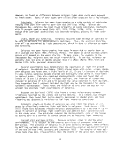 g g
SNOI10VHJ 0 iN33a3d
(%) M31.WH
1V.L01
(0)iN3IOIdJ300
9NI1HOS 1N3WIQ3S
1N3HI03S NVI03W
<XJ
(O
s_
<D
5
-o
a>
CO
fO
CO
c
3
-©-
c
OJ
I/I
01
CL
res
CO
o e
2 CM
+J CD
II
<1)
01 -r-
c x:
<a a.
M
-a
ta
a>
s:
re
cu
s-
Ol
o
.a
fO
ID
ra
10
CO
o
o
fO
CO
o
s
O)
CO
S-
<a
x:
o
•o
(U
to
CTi
OJ
3
a>
40
image:
g g
SNOI10VHJ 0 iN33a3d
(%) M31.WH
1V.L01
(0)iN3IOIdJ300
9NI1HOS 1N3WIQ3S
1N3HI03S NVI03W
<XJ
(O
s_
<D
5
-o
a>
CO
fO
CO
c
3
-©-
c
OJ
I/I
01
CL
res
CO
o e
2 CM
+J CD
II
<1)
01 -r-
c x:
<a a.
M
-a
ta
a>
s:
re
cu
s-
Ol
o
.a
fO
ID
ra
10
CO
o
o
fO
CO
o
s
O)
CO
S-
<a
x:
o
•o
(U
to
CTi
OJ
3
a>
40
image:
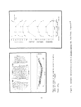 in exposed areas, indicating a greater intensity of erosional activity along
these edges (Hartog 1970; Orth and Gordon 1975).
Along the bayside of the Delmarva Peninsula, Virginia, the presence of an
extensive offshore intertidal sand bar allows the development of eel grass beds
behind the bars, by reducing wave activity from offshore winds. Intertidal
sand bars interspersed with eel grass between the bars are features typical of
some exposed areas in the Chesapeake Bay (Orth 1975b; Orth and Gordon 1975)
and the persistence of these sand bars is probably related to the hydrodynamics
and bottom topography of the region. As with the offshore bar, the presence of
these smaller sand bars allows the growth of eelgrass by reduci'nq wave activity.
Current itself apparently is important to the growth of ee'lgrass. Phillips
(1974a_) found luxuriant eelgrass where currents reached speeds up to 3.5 knots.
Conover (1958, 1968) found similar results for eelgrass in Rhode Island and
Massachusetts. He showed that gross and net production rates cou'ld be raised or
lowered by changing the recirculation velocity of the seawater in experimental
tanks. Eelgrass attained peak biomass figures in current cpeeds of around one
knot with a sharp dropoff above this figure. The connection between current
velocity and plant metabolic rates is believed to be a function of the rate of
transfer of required gaseous and dissolved nutrients from the water into the
organisms.
Sedimentation. As mentioned in the previous section, eelgrass has the
ability to trap and bind sediments, providing some stability to the bottom
substrate. This trapping effect usually results in a slight elevation of the
eelgrass bed above the surrounding unvegetated bottom (Hartog 1979; Orth,
personal observation). In some areas, movement of sand may be so great, e.g.
during periods of intense storm activity, as to actually cover the grass thereby
killing it. Blois et al.(1971, cited in Hartog 1970) described this phenomena
to occur in one day. However, they observed new rhizome growth in the sanded
area resulting in a new horizon of rhizomes. In one Zostera bed they found seven
separate rhizome layers. In one location in the Chesapeake Bay, Orth (personal
observation) found an edge of a sand bar migrating across an eelgrass bed.
Recently covered grass that was still green was observed 20 cm or more beneath
the surface of the sand.
Some areas in the Bay have characteristic sand bars parallel to the shore
with slight depressions between the bars. In some areas, these depressions are
inhabited by eelgrass and the trapping and binding properties of eelgrass are
evident here also (see Figure 9). Sediments just inside the grass bed are
distinctly different from those immediately outside the bed and they <;jet pro-
gressively finer from the edge to the center of the bed.
Susceptibility. Because eelgrass lives in an aquatic environment,,, it is
subject to pollutants from both point and non-point sources. Unfortunately,
there is very little information concerning the effects of various toxicants
on the growth and survival of eelgrass.
Thomas (1967) and Thomas and Duffy (1968) tested the effect of nine dif-
ferent herbicides on the growth of eelgrass (see Table 5). They found that
41
image:
in exposed areas, indicating a greater intensity of erosional activity along
these edges (Hartog 1970; Orth and Gordon 1975).
Along the bayside of the Delmarva Peninsula, Virginia, the presence of an
extensive offshore intertidal sand bar allows the development of eel grass beds
behind the bars, by reducing wave activity from offshore winds. Intertidal
sand bars interspersed with eel grass between the bars are features typical of
some exposed areas in the Chesapeake Bay (Orth 1975b; Orth and Gordon 1975)
and the persistence of these sand bars is probably related to the hydrodynamics
and bottom topography of the region. As with the offshore bar, the presence of
these smaller sand bars allows the growth of eelgrass by reduci'nq wave activity.
Current itself apparently is important to the growth of ee'lgrass. Phillips
(1974a_) found luxuriant eelgrass where currents reached speeds up to 3.5 knots.
Conover (1958, 1968) found similar results for eelgrass in Rhode Island and
Massachusetts. He showed that gross and net production rates cou'ld be raised or
lowered by changing the recirculation velocity of the seawater in experimental
tanks. Eelgrass attained peak biomass figures in current cpeeds of around one
knot with a sharp dropoff above this figure. The connection between current
velocity and plant metabolic rates is believed to be a function of the rate of
transfer of required gaseous and dissolved nutrients from the water into the
organisms.
Sedimentation. As mentioned in the previous section, eelgrass has the
ability to trap and bind sediments, providing some stability to the bottom
substrate. This trapping effect usually results in a slight elevation of the
eelgrass bed above the surrounding unvegetated bottom (Hartog 1979; Orth,
personal observation). In some areas, movement of sand may be so great, e.g.
during periods of intense storm activity, as to actually cover the grass thereby
killing it. Blois et al.(1971, cited in Hartog 1970) described this phenomena
to occur in one day. However, they observed new rhizome growth in the sanded
area resulting in a new horizon of rhizomes. In one Zostera bed they found seven
separate rhizome layers. In one location in the Chesapeake Bay, Orth (personal
observation) found an edge of a sand bar migrating across an eelgrass bed.
Recently covered grass that was still green was observed 20 cm or more beneath
the surface of the sand.
Some areas in the Bay have characteristic sand bars parallel to the shore
with slight depressions between the bars. In some areas, these depressions are
inhabited by eelgrass and the trapping and binding properties of eelgrass are
evident here also (see Figure 9). Sediments just inside the grass bed are
distinctly different from those immediately outside the bed and they <;jet pro-
gressively finer from the edge to the center of the bed.
Susceptibility. Because eelgrass lives in an aquatic environment,,, it is
subject to pollutants from both point and non-point sources. Unfortunately,
there is very little information concerning the effects of various toxicants
on the growth and survival of eelgrass.
Thomas (1967) and Thomas and Duffy (1968) tested the effect of nine dif-
ferent herbicides on the growth of eelgrass (see Table 5). They found that
41
image:
 *d
LO
4-3
c
QJ
gr
•r—
t.
cu
Q.
X
cu
, —
o
S-
•*->
E
O
0
to
re
CO
"cu
O)
^_
'o
CO
-(->
r~
3
CO
cu
s-
E
•r—
re
•^j
E
re
-o
cu
CO
3
CO
E
O
•r-
-^*
re
4J
E
CU
o
E
O
u
f
T3
CU
4J
to
CU
to
re
o
'i
CU
c™
I—
0
•
LO
CU
r—
f">
re
I—
to
4_>
r~.
^25
to
CU
fV
4_>
E
O) CU
> T-
•r- -0
.— ( 4-* QJ
2 0 S-
:r < CO
to *"•
cu -I~
re
i_
E
Q
, ^
frt ^
(w -_
OO
,
1H +->
Q. re
5" |
5^.
o
LJ_
CU
£
E
r—
re
o
• r—
£
CU
_E
CJ
1 —
re
o
'i
cu
c**
o
cu
E
re
E
CU
-o
re
s-
h-
i —
n3
C"
^
re
(4—
CU
g^
o
to
N. ^
cu cu
E E
O O
"^ "^
CO CO
O 0
CM CM
1 1
LO LO
• •
O O
S- S_
cu cu
4_> 4-i
•r™ *f_
r— 1— —
CO CO
• »
CO CO
00 00
1 1
o^ o^
• •
I— r—
,^— %
i.
,— , CU
t- -4- '
CU -r-
1 ^ ^
i— co
"^ *^
CO
-ii CM
O
CM •
0 O
• V ^
o
^ , j \
re
+-> 3
re cr
3 re
cr s-
•t- 03
Q 0-
CU
E
CU O
E X
O O
i— E
co re
CU i-
cc o
i— tO
r— S-
re cu
-t~>
4- to
0 >,
O
>^
^_> ^_>
•r- Q.
r— CU
re o
-M X
s- cu
o
E CU
r— O
re v-
4~) o
O
1—
S-
eu
^_3
•r—
n—
i^—
r^.
i-^
S-
cu
i^I
to
en
f~>
i
X
CD
i—
t-~ <
•i—
S-
Q
CU
E
O
"5*"
CD
^y
CO
CM
^"
1
C\J
r—
i —
01
J$£
vo
oo
r—
1
O
•
CTi
•=^-
s~ -*+
is*.
oo
CM
^ *•
X
a;
r—
•r-.
00
r n
f—
re
to
o
s-
3
^
CU
E
O
^^
j
CO
\/
p-^.
LO
r-.
1
CM
•
to
OO
co
^
CO
CO
1
LO
en
•—
, — ^
^-^
LO
^ — *
r-—
re
40
o
•73
E
UJ
r-^
O
_c
40
«J
3
o-
4_)
03
i—
,—
•i —
-^
^5,
r- CU
E re
re s-
.E
4_> •
X
to re
to E
cu
i
CO
sx
to
•
oo
VO
1
CO
•
r—
CO
CD
,,.yf
^*
CT»
LO
1
r^*.
O"^
CM
x1 s.,^ -s
^5 S1^
r— VO
• •
LO LO
*• — -•*- — -*
r- X
re cu
-E >
-4—^ r—
O •!-
T3 OO
E
LU
to
i — 3
0 •—
-E D-
4«^
re
3
CT
ef
CU
E
O
^^
CD
,^|
i—
•
O"i
CO
i
CM
•
^"
CM
CD
^^,
o
r—
r^
i
o
^~
•*
^— ^
^^
LO
•
LO
x ^
O
re
E
CU
CJ3
LO
O
re
E
CU
LJ_
' ^
cu
4-> QJ
fO 4->
s_ re
S-
•
X •
re E
E T-
E
4-)
ns 4->
re
^^
o cu
O E
r— O
1 E
0
LO
CO
-^
^O
•
r^.
CM
,—
1
CO
•
CM
CO
_v
o
^J-
"vt-
1
fv».
^j-
<—
•~-~^
^^
o^
CM
^_^
Q
1
<sj-
*»
CM
C
CU
cu
r—
S/^
1
rT3
Z5
cr
. ^
OJ
4-* QJ
(0 +^
s- re
i.
.
x •
re E
E T-
E
10 -)->
re
o &s
en LO
1 CM
o
LO
CO
\s
^~
•
CM
CM
1
«sj-
•
1 — ^
CO
VX
O
LO
LO
1
p*^
CO
<—
, — ,
<3~^
^J-
*. — ^
r—
• r-
E
CU
J2
o
s-
o
^^
_c
u
•r~
o
^-
crs
E
O
0
to
re
o
cj^
o
o
1
o
en
CO
\s
en
oo
i
LO
>^f
CO
\x
to
•=3-
1
OO
CM
CM
^ — ^
^Q
en
CM
v — -•
i ^
i
«sj-
n
CM
E
CU
CU
r—~
^S
|
re
3
cr
<C
O)
E
O
SZ
cn
_^
to
px^.
r—
1
r*^».
•
r^.
en
\s
to
^j-
«^J-
1
O
o
CM
, — ^
c3-*i
^J-
^ — ••
r^*
• r—
E
CU
o
O
O
r-~
-E
U
•r—
Q
to
*=j- en
CJ3 •—
E tO
o re
S- E
O O
tO -E
re h-
cj> to
image:
*d
LO
4-3
c
QJ
gr
•r—
t.
cu
Q.
X
cu
, —
o
S-
•*->
E
O
0
to
re
CO
"cu
O)
^_
'o
CO
-(->
r~
3
CO
cu
s-
E
•r—
re
•^j
E
re
-o
cu
CO
3
CO
E
O
•r-
-^*
re
4J
E
CU
o
E
O
u
f
T3
CU
4J
to
CU
to
re
o
'i
CU
c™
I—
0
•
LO
CU
r—
f">
re
I—
to
4_>
r~.
^25
to
CU
fV
4_>
E
O) CU
> T-
•r- -0
.— ( 4-* QJ
2 0 S-
:r < CO
to *"•
cu -I~
re
i_
E
Q
, ^
frt ^
(w -_
OO
,
1H +->
Q. re
5" |
5^.
o
LJ_
CU
£
E
r—
re
o
• r—
£
CU
_E
CJ
1 —
re
o
'i
cu
c**
o
cu
E
re
E
CU
-o
re
s-
h-
i —
n3
C"
^
re
(4—
CU
g^
o
to
N. ^
cu cu
E E
O O
"^ "^
CO CO
O 0
CM CM
1 1
LO LO
• •
O O
S- S_
cu cu
4_> 4-i
•r™ *f_
r— 1— —
CO CO
• »
CO CO
00 00
1 1
o^ o^
• •
I— r—
,^— %
i.
,— , CU
t- -4- '
CU -r-
1 ^ ^
i— co
"^ *^
CO
-ii CM
O
CM •
0 O
• V ^
o
^ , j \
re
+-> 3
re cr
3 re
cr s-
•t- 03
Q 0-
CU
E
CU O
E X
O O
i— E
co re
CU i-
cc o
i— tO
r— S-
re cu
-t~>
4- to
0 >,
O
>^
^_> ^_>
•r- Q.
r— CU
re o
-M X
s- cu
o
E CU
r— O
re v-
4~) o
O
1—
S-
eu
^_3
•r—
n—
i^—
r^.
i-^
S-
cu
i^I
to
en
f~>
i
X
CD
i—
t-~ <
•i—
S-
Q
CU
E
O
"5*"
CD
^y
CO
CM
^"
1
C\J
r—
i —
01
J$£
vo
oo
r—
1
O
•
CTi
•=^-
s~ -*+
is*.
oo
CM
^ *•
X
a;
r—
•r-.
00
r n
f—
re
to
o
s-
3
^
CU
E
O
^^
j
CO
\/
p-^.
LO
r-.
1
CM
•
to
OO
co
^
CO
CO
1
LO
en
•—
, — ^
^-^
LO
^ — *
r-—
re
40
o
•73
E
UJ
r-^
O
_c
40
«J
3
o-
4_)
03
i—
,—
•i —
-^
^5,
r- CU
E re
re s-
.E
4_> •
X
to re
to E
cu
i
CO
sx
to
•
oo
VO
1
CO
•
r—
CO
CD
,,.yf
^*
CT»
LO
1
r^*.
O"^
CM
x1 s.,^ -s
^5 S1^
r— VO
• •
LO LO
*• — -•*- — -*
r- X
re cu
-E >
-4—^ r—
O •!-
T3 OO
E
LU
to
i — 3
0 •—
-E D-
4«^
re
3
CT
ef
CU
E
O
^^
CD
,^|
i—
•
O"i
CO
i
CM
•
^"
CM
CD
^^,
o
r—
r^
i
o
^~
•*
^— ^
^^
LO
•
LO
x ^
O
re
E
CU
CJ3
LO
O
re
E
CU
LJ_
' ^
cu
4-> QJ
fO 4->
s_ re
S-
•
X •
re E
E T-
E
4-)
ns 4->
re
^^
o cu
O E
r— O
1 E
0
LO
CO
-^
^O
•
r^.
CM
,—
1
CO
•
CM
CO
_v
o
^J-
"vt-
1
fv».
^j-
<—
•~-~^
^^
o^
CM
^_^
Q
1
<sj-
*»
CM
C
CU
cu
r—
S/^
1
rT3
Z5
cr
. ^
OJ
4-* QJ
(0 +^
s- re
i.
.
x •
re E
E T-
E
10 -)->
re
o &s
en LO
1 CM
o
LO
CO
\s
^~
•
CM
CM
1
«sj-
•
1 — ^
CO
VX
O
LO
LO
1
p*^
CO
<—
, — ,
<3~^
^J-
*. — ^
r—
• r-
E
CU
J2
o
s-
o
^^
_c
u
•r~
o
^-
crs
E
O
0
to
re
o
cj^
o
o
1
o
en
CO
\s
en
oo
i
LO
>^f
CO
\x
to
•=3-
1
OO
CM
CM
^ — ^
^Q
en
CM
v — -•
i ^
i
«sj-
n
CM
E
CU
CU
r—~
^S
|
re
3
cr
<C
O)
E
O
SZ
cn
_^
to
px^.
r—
1
r*^».
•
r^.
en
\s
to
^j-
«^J-
1
O
o
CM
, — ^
c3-*i
^J-
^ — ••
r^*
• r—
E
CU
o
O
O
r-~
-E
U
•r—
Q
to
*=j- en
CJ3 •—
E tO
o re
S- E
O O
tO -E
re h-
cj> to
image:
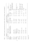 only dichlobenil and 2,4-D had any effect on eelgrass and further testing
showed 2,4-D to be extremely toxic. Areas killed by 2,4-D ranged from 3.2 to
5.8 times the area treated because of current-born herbicide.
Nutrient Response. Nutrient cycles in eelgrass beds are complex and the
problems associated with nutrient limitation, sites and rates of uptake still
need further investigation. Recent work has shown that eelgrass can absorb
phosphorus and nitrogen across the leaves and roots and transport it to other
parts of the pTant (McRoy and Barsdate 1970; McRoy et al. 1972; McRoy et al.
1973; Barsdate et al. 1974; Penhale 1976). Eelgrass also serves as a "nutrient
pump", pumping phosphate and ammonia from the sediments through the plant and
releasing them into the water. The flow of phosphorus can occur in the opposite
direction, but the net effect is to transport phosphorus from the sediment to
the water, effectively increasing the concentration of these nutrients in the
water.
This transport of nutrients is very important to epiphytic algae because
they apparently utilize carbon, nitrogen and phosphorus excreted by the plant
(Harlin 1971; McRoy and Goering 1974; Penhale 1976). This would potentially
allow greater growths of algae on grass blades in nutrient poor water than
otherwise possible.
Little work has been conducted with nutrient enrichment studies. Raymont
(1947) and Marshall and Orr (1948) studied the effects of the addition of fer-
tilizers (sodium nitrate and superphosphate) to sea lochs, primarly to study
the effects on algal primary productivity and resultant fish production. They
noticed an increased abundance of eelgrass but no actual measurements were made
of this increase, nor were appropriate controls available (i.e. they did not
differentiate normal seasonal growth from growth presumably enhanced by fer-
tilizing). Marshall and Orr suspected that eelgrass utilized the added nutrients
before the phytoplankton. Orth (in press) working in a more controlled experi-
ment off Hungers Creek, Delmarva Peninsula, found that the biomass, length and
number of vegetative turions of eelgrass increased significantly when commercial
fertilizer was added to sediments in an eelgrass bed (see Figure 10). Fertili-
zers with N-P-K values of 5-10-10 and 10-10-10 were used.
Eelgrass appears to be very effective in concentrating various elements
from the water (e.g. major elements such as carbon, nitrogen and phosphorus,
minor elements such as manganese, aluminum and iron, and trace elements such as
copper, cobalt and beryllium) including radioactive isotopes (McRoy 1970lb;
Barsdate et al. 1974). The "accumulation of elements in eelgrass is proportional
to the abundance of an element in the water. Thus, it would appear that any
increase in a major element would be reflected in eelgrass.
Productivity
Table 6 summarizes the available information on productivity measurements
for eelgrass. Data on standing stock (g/m2 dry weight) and productivity
(g C/m2/day) of eelgrass at different localities vary widely, ranging 1 to 5157
and 0.04 to 8, respectively. Turion density is also highly variable. The ranges
found in Table 6 for those parameters probably correlate with the diverse mor-
phology observed for eelgrass in environmentally different yet often geograph-
ically close areas. Considerable attention is necessary when comparing these
43
image:
only dichlobenil and 2,4-D had any effect on eelgrass and further testing
showed 2,4-D to be extremely toxic. Areas killed by 2,4-D ranged from 3.2 to
5.8 times the area treated because of current-born herbicide.
Nutrient Response. Nutrient cycles in eelgrass beds are complex and the
problems associated with nutrient limitation, sites and rates of uptake still
need further investigation. Recent work has shown that eelgrass can absorb
phosphorus and nitrogen across the leaves and roots and transport it to other
parts of the pTant (McRoy and Barsdate 1970; McRoy et al. 1972; McRoy et al.
1973; Barsdate et al. 1974; Penhale 1976). Eelgrass also serves as a "nutrient
pump", pumping phosphate and ammonia from the sediments through the plant and
releasing them into the water. The flow of phosphorus can occur in the opposite
direction, but the net effect is to transport phosphorus from the sediment to
the water, effectively increasing the concentration of these nutrients in the
water.
This transport of nutrients is very important to epiphytic algae because
they apparently utilize carbon, nitrogen and phosphorus excreted by the plant
(Harlin 1971; McRoy and Goering 1974; Penhale 1976). This would potentially
allow greater growths of algae on grass blades in nutrient poor water than
otherwise possible.
Little work has been conducted with nutrient enrichment studies. Raymont
(1947) and Marshall and Orr (1948) studied the effects of the addition of fer-
tilizers (sodium nitrate and superphosphate) to sea lochs, primarly to study
the effects on algal primary productivity and resultant fish production. They
noticed an increased abundance of eelgrass but no actual measurements were made
of this increase, nor were appropriate controls available (i.e. they did not
differentiate normal seasonal growth from growth presumably enhanced by fer-
tilizing). Marshall and Orr suspected that eelgrass utilized the added nutrients
before the phytoplankton. Orth (in press) working in a more controlled experi-
ment off Hungers Creek, Delmarva Peninsula, found that the biomass, length and
number of vegetative turions of eelgrass increased significantly when commercial
fertilizer was added to sediments in an eelgrass bed (see Figure 10). Fertili-
zers with N-P-K values of 5-10-10 and 10-10-10 were used.
Eelgrass appears to be very effective in concentrating various elements
from the water (e.g. major elements such as carbon, nitrogen and phosphorus,
minor elements such as manganese, aluminum and iron, and trace elements such as
copper, cobalt and beryllium) including radioactive isotopes (McRoy 1970lb;
Barsdate et al. 1974). The "accumulation of elements in eelgrass is proportional
to the abundance of an element in the water. Thus, it would appear that any
increase in a major element would be reflected in eelgrass.
Productivity
Table 6 summarizes the available information on productivity measurements
for eelgrass. Data on standing stock (g/m2 dry weight) and productivity
(g C/m2/day) of eelgrass at different localities vary widely, ranging 1 to 5157
and 0.04 to 8, respectively. Turion density is also highly variable. The ranges
found in Table 6 for those parameters probably correlate with the diverse mor-
phology observed for eelgrass in environmentally different yet often geograph-
ically close areas. Considerable attention is necessary when comparing these
43
image:
 STATION A
STATION B
600-
300-
• 400
300
200
2
3
z 100-
_J
»-
0
40-
7
0
5 30-
o
K
X
H
o
z
_J
z
U)
40
N
E
£30-
m
Ul
520-
u
_J
0
« 10-
to
4
5-
o
2 _
0-
(
I ^
_L
/X
APRIL 13 JUNE 22
<
~T"
UL
^ o^^o
APRIL 13 JUNE 22
-1
<
_
T
I
^ >«
<£? •>' $
APRIL 13 JUNE 22
<
)
/
-3
/
r
' I
L ,
<
.
>°
'
'
1
r
'
.
IT
1 i f
-0^ -P' x«
^ .* >°
APRIL 13 JULY 8
ll
I
^V'o'*'
APRIL 13 JULY •
-p
I"
--
5
^ ,* >*'
<j? V5*^
APRIL 13 JULY •
600
•MM
•4OO
SOO
•ZOO
•100
40
30
• 20
10
40
30
•20
•10
STATION A
STATION •
Figure 10. Effect of the addition of fertilizers
5-10-10 and 10-10-10 on the growth of Zostera
marina
44
image:
STATION A
STATION B
600-
300-
• 400
300
200
2
3
z 100-
_J
»-
0
40-
7
0
5 30-
o
K
X
H
o
z
_J
z
U)
40
N
E
£30-
m
Ul
520-
u
_J
0
« 10-
to
4
5-
o
2 _
0-
(
I ^
_L
/X
APRIL 13 JUNE 22
<
~T"
UL
^ o^^o
APRIL 13 JUNE 22
-1
<
_
T
I
^ >«
<£? •>' $
APRIL 13 JUNE 22
<
)
/
-3
/
r
' I
L ,
<
.
>°
'
'
1
r
'
.
IT
1 i f
-0^ -P' x«
^ .* >°
APRIL 13 JULY 8
ll
I
^V'o'*'
APRIL 13 JULY •
-p
I"
--
5
^ ,* >*'
<j? V5*^
APRIL 13 JULY •
600
•MM
•4OO
SOO
•ZOO
•100
40
30
• 20
10
40
30
•20
•10
STATION A
STATION •
Figure 10. Effect of the addition of fertilizers
5-10-10 and 10-10-10 on the growth of Zostera
marina
44
image:
 to ro
>>io
rO Ol
8
I
QJ
CM >>
r^. c N
Ol OJ 4->
,81
O) QJ QJ O
•*-> i_ I O !/>
C QJ T3 -4-* C
CD Q. (/) CD O
> > C -C p r—
3E <3 O Z
I •«- 10 VO
3 i- §£ 2g""
- oj*>-"_^ ro
•— CLr— r—
- "O i— O O (O
O f> -r-
Q. +J >
-_
D. (— ^C
•U 01
*> W
Si1
1
ro i r—
O Or
ro LO ro
o o o
21=
8
o o o
Oi CO CO
<v> CM i—
ro o Oi
i— Ol
r-. m
ro m
CM CO
r-. m o
CM m o
in CM ^j-
trt
(-
: Oi
o oo moo"^ cor->
ICM'i— ICM « .Ol • f^.
r- O CM \£> CO Ol IT) CM
^— lO CO i— \O
0
Ol
c\j«3-roioos
COOOCMOCO^IDOCOO
u-jr-cMoicM'sfcoroooLn
i — CM^-I — ^f^Di — CMOICMI —
in 01 vo • —
Ol S-
•— 0)
e"
Q.-P-
go
CO -M -O -O
(O fO -4-> C C
r-— «i— Q) fO rO
tfl 4-> W •— !—j:
CO DQ CO t- -I— T- -I— -i— •(—
Q) p— .— p- r— r- L) JD
>>a)<l)Q)>OOOOOrOraC
<O ra
C OJ QJ
•p- (/) C/)
o <u o E
S-r- E O
4- Q. o in
E i/) J=
•a ro <u .c Q-
QJ Ul O •*-» ro
•M T3 T- t-
O >, X 0>
QJ r- S-
t.^: OT3 E
S- -M QJ O
O C O1.C i-
O O C (J«-
"o i— r —
C i. Q.
rO O E
"O i— tfl trt i—
QJ ro (OO
-f- C 1- ro Q.
M- O OJ S. t-
•p- Wl E Ol QJ
O OJ 3 QJ C
E tO IO UJ »-H
fO -Q U "O QJ
45
image:
to ro
>>io
rO Ol
8
I
QJ
CM >>
r^. c N
Ol OJ 4->
,81
O) QJ QJ O
•*-> i_ I O !/>
C QJ T3 -4-* C
CD Q. (/) CD O
> > C -C p r—
3E <3 O Z
I •«- 10 VO
3 i- §£ 2g""
- oj*>-"_^ ro
•— CLr— r—
- "O i— O O (O
O f> -r-
Q. +J >
-_
D. (— ^C
•U 01
*> W
Si1
1
ro i r—
O Or
ro LO ro
o o o
21=
8
o o o
Oi CO CO
<v> CM i—
ro o Oi
i— Ol
r-. m
ro m
CM CO
r-. m o
CM m o
in CM ^j-
trt
(-
: Oi
o oo moo"^ cor->
ICM'i— ICM « .Ol • f^.
r- O CM \£> CO Ol IT) CM
^— lO CO i— \O
0
Ol
c\j«3-roioos
COOOCMOCO^IDOCOO
u-jr-cMoicM'sfcoroooLn
i — CM^-I — ^f^Di — CMOICMI —
in 01 vo • —
Ol S-
•— 0)
e"
Q.-P-
go
CO -M -O -O
(O fO -4-> C C
r-— «i— Q) fO rO
tfl 4-> W •— !—j:
CO DQ CO t- -I— T- -I— -i— •(—
Q) p— .— p- r— r- L) JD
>>a)<l)Q)>OOOOOrOraC
<O ra
C OJ QJ
•p- (/) C/)
o <u o E
S-r- E O
4- Q. o in
E i/) J=
•a ro <u .c Q-
QJ Ul O •*-» ro
•M T3 T- t-
O >, X 0>
QJ r- S-
t.^: OT3 E
S- -M QJ O
O C O1.C i-
O O C (J«-
"o i— r —
C i. Q.
rO O E
"O i— tfl trt i—
QJ ro (OO
-f- C 1- ro Q.
M- O OJ S. t-
•p- Wl E Ol QJ
O OJ 3 QJ C
E tO IO UJ »-H
fO -Q U "O QJ
45
image:
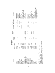 studies; some numbers represent samples from seasonal studies, where the range
of values will be greater than those from studies where samples were only col-
lected during the season of maximal biomass. Sampling techniques vary widely,
especially in productivity studies, and make it difficult to draw distinct con-
clusions.
Eelgrass is a temperate seagrass and has a distinct growing season. Maxi-
mal biomass of leaves is normally attained from June through August (Penhale
(1977 found this in March) while minimal biomass is attained during January
and February.
Consumer Utilization
Despite the abundance of eel grass along the coast, there are relatively
few animals that directly utilize the grass as a food course. However, this
fact alone does not belie the importance of eel grass as a habitat and nursery
for many forms of invertebrates and vertebrates, both juveniles and adults.
These organisms often undoubtedly serve as a source of food of species at higher
trophic levels.
The fauna and flora of eelgrass beds can be divided into several cate-
gories: the epibiota (animals and plants utilizing the blades of eelgrass as
a substrate), the infauna, (animals found on or in the sediments) and the motile
invertebrates and vertebrates. Within this last group there can be subgroups
such as permanent residents, seasonal residents, transients which utilize a
wider area than the seagrass bed and occasional migrants.
The epibiota and infauna represent a diverse and complex assemblage which
includes micro- and macroalgae, protozoans, hydrozoans, anthozoans, turbellarians,
gastropods, isopods, amphipods, polychaetes, oligochaetes, bivalves, decapods
and barnacles. Many of these groups exhibit distinct seasonal pulses of abun-
dance depending on their individual spawning periods (Barnard 1970; Kikuchi 1968;
Kikuchi and Peres 1977; Lappalainen 1973; Lappalainen and Kangas 1975; Levinton
1977; Levinton and Bambach 1975; Marsh 1970, 1973, 1976; Nagle 1968; Orth 1971,
1973, 1975a_, 1975^, 1977a_,lb; Rasmussen 1973; Thayer et al. 1975).
The biotic community within grass beds is quite distinct from the commun-
ities in adjacent unvegetated areas. Because of the lack of suitable substratum,
there is usually very little epifauna in bare sand or mud areas. The animals
are primarily using blades as a substratum or in the case of herbivorous
gastropods, grazing on the microalgae that grow on the blades. In experiments
where artifical grasses were used, an epifaunal community similar to that found
on the real seagrass developed on the artificial seagrass (Moulton 1971; Orth,
unpublished data).
The infaunal community is also quite distinct from adjacent unvegetated
areas. There is a tremendous increase in numbers of species and individuals in
grass areas and this may be related to increased sediment stability, micro-
habitat complexity of food supply (Kikuchi 1966; Williams and Thomas 1967;
Nilsson 1969; Adams and Angelovic 1970; Tenore 1975; Orth 1975^, 1977b/, Thayer
et al. 1975). Orth (1975^, 19775.) working with infauna of Chesapeake Bay eel-
grass, found infauna to increase in density and diversity from the edge of an
46
image:
studies; some numbers represent samples from seasonal studies, where the range
of values will be greater than those from studies where samples were only col-
lected during the season of maximal biomass. Sampling techniques vary widely,
especially in productivity studies, and make it difficult to draw distinct con-
clusions.
Eelgrass is a temperate seagrass and has a distinct growing season. Maxi-
mal biomass of leaves is normally attained from June through August (Penhale
(1977 found this in March) while minimal biomass is attained during January
and February.
Consumer Utilization
Despite the abundance of eel grass along the coast, there are relatively
few animals that directly utilize the grass as a food course. However, this
fact alone does not belie the importance of eel grass as a habitat and nursery
for many forms of invertebrates and vertebrates, both juveniles and adults.
These organisms often undoubtedly serve as a source of food of species at higher
trophic levels.
The fauna and flora of eelgrass beds can be divided into several cate-
gories: the epibiota (animals and plants utilizing the blades of eelgrass as
a substrate), the infauna, (animals found on or in the sediments) and the motile
invertebrates and vertebrates. Within this last group there can be subgroups
such as permanent residents, seasonal residents, transients which utilize a
wider area than the seagrass bed and occasional migrants.
The epibiota and infauna represent a diverse and complex assemblage which
includes micro- and macroalgae, protozoans, hydrozoans, anthozoans, turbellarians,
gastropods, isopods, amphipods, polychaetes, oligochaetes, bivalves, decapods
and barnacles. Many of these groups exhibit distinct seasonal pulses of abun-
dance depending on their individual spawning periods (Barnard 1970; Kikuchi 1968;
Kikuchi and Peres 1977; Lappalainen 1973; Lappalainen and Kangas 1975; Levinton
1977; Levinton and Bambach 1975; Marsh 1970, 1973, 1976; Nagle 1968; Orth 1971,
1973, 1975a_, 1975^, 1977a_,lb; Rasmussen 1973; Thayer et al. 1975).
The biotic community within grass beds is quite distinct from the commun-
ities in adjacent unvegetated areas. Because of the lack of suitable substratum,
there is usually very little epifauna in bare sand or mud areas. The animals
are primarily using blades as a substratum or in the case of herbivorous
gastropods, grazing on the microalgae that grow on the blades. In experiments
where artifical grasses were used, an epifaunal community similar to that found
on the real seagrass developed on the artificial seagrass (Moulton 1971; Orth,
unpublished data).
The infaunal community is also quite distinct from adjacent unvegetated
areas. There is a tremendous increase in numbers of species and individuals in
grass areas and this may be related to increased sediment stability, micro-
habitat complexity of food supply (Kikuchi 1966; Williams and Thomas 1967;
Nilsson 1969; Adams and Angelovic 1970; Tenore 1975; Orth 1975^, 1977b/, Thayer
et al. 1975). Orth (1975^, 19775.) working with infauna of Chesapeake Bay eel-
grass, found infauna to increase in density and diversity from the edge of an
46
image:
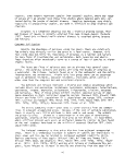 eelgrass bed to the center of the bed (see Figure 11) and also with increasing
size of the bed (see Figure 12). He related this increase to the sediment
stability component of eelgrass and showed that decreasing the stability of
sediments experimentally (removing blades of grass by clipping, simulating wave
action) and naturally (cownose ray activity (Orth 1975-a)), decreased the density
and diversity of the infauna.
The motile community is also diverse and quite distinct from surrounding
unvegetated areas (Orth and Heck, unpublished; Briggs and O'Conner 1971; Kikuchi
1974b). Utilization of these grass areas by fish and invertebrates may be for
distinctly different reasons. Hartfwick (1973) found that on the West Coast,
the herring (Clupea harengus pallasi) used eelgrass leaves to lay most of their
eggs. Juveniles and adults of many species may utilize eelgrass for protection.
The blue crab (Callinectes sapidus) is found in greater abundance in eelgrass
both as juveniles and adults (Lippson 1970; Sulkin 1973, 1977; Orth and Heck,
unpublished). Many species may use eelgrass beds primarily as a habitat and
feeding ground because of the abundance of food. Barry (1974) found shrimp,
(Hippolyte californiensis) which inhabit eelgrass beds on the West Coast, were
able to recognize the leaves of eelgrass by discriminating it on the basis of
its form.
One of the more complete studies of fish communities of eelgrass was done
by Adams (1976c[, 1976t^, 1976cJ. He found the highest fish biomass when tempera-
ture and eelgrass biomass were maximal. Further, food produced within the grass
bed could have accounted for approximately 56 percent by weight of the diet of
the fish community. The high fish production was due to juveniles which had
higher growth efficiences than older fishes. They accounted for 79 to 84 percent
of the total annual fish production.
The only groups of animals that consume eelgrass directly are waterfowl and
sea turtles. Cottam (1934bJ stated that eelgrass made up 80 percent of the
winter food of Sea Brant and that Canada Geese, Scaups, Redheads and Black ducks
consumed considerable quantities of eelgrass (Addy and Aylward 1944).
Human consumption of eelgrass has been found among the Seri Indians in the
Gulf of California (Felger and Moser 1973). They would harvest the seed and pre-
pare a gruel which is eaten with other food. Felger and McRoy (1975) made bread
from the flour and found the bread "had a good flavor when fresh, and is somewhat
like rye bread."
The importance of eelgrass as a habitat became more evident after its de-
cline in the early 1930s. Stauffer (1937) reported a decline of 33 percent of
the characteristic species normally found in eelgrass after the demise. There
were sharp declines in waterfowl populations. Urner (1934) reported that
Canada Geese and Brant declined by 75 percent and 92 percent, respectively, in
New Jersey. Similar declines for these species and other waterfowl were re-
ported from Europe (Bruijns and Tanis 1955; Ranwell and Downing 1959) and other
sections of the United States (Moffit and Cottam 1941).
Another serious effect was on the bay scallop (Aequipecten irradians) popu-
lation on the Eastern Shore of Virginia. The commercial fishery that amounted
to a harvest of over 14,000 kg/year in the late 1920s and early 1930s was reduced
47
image:
eelgrass bed to the center of the bed (see Figure 11) and also with increasing
size of the bed (see Figure 12). He related this increase to the sediment
stability component of eelgrass and showed that decreasing the stability of
sediments experimentally (removing blades of grass by clipping, simulating wave
action) and naturally (cownose ray activity (Orth 1975-a)), decreased the density
and diversity of the infauna.
The motile community is also diverse and quite distinct from surrounding
unvegetated areas (Orth and Heck, unpublished; Briggs and O'Conner 1971; Kikuchi
1974b). Utilization of these grass areas by fish and invertebrates may be for
distinctly different reasons. Hartfwick (1973) found that on the West Coast,
the herring (Clupea harengus pallasi) used eelgrass leaves to lay most of their
eggs. Juveniles and adults of many species may utilize eelgrass for protection.
The blue crab (Callinectes sapidus) is found in greater abundance in eelgrass
both as juveniles and adults (Lippson 1970; Sulkin 1973, 1977; Orth and Heck,
unpublished). Many species may use eelgrass beds primarily as a habitat and
feeding ground because of the abundance of food. Barry (1974) found shrimp,
(Hippolyte californiensis) which inhabit eelgrass beds on the West Coast, were
able to recognize the leaves of eelgrass by discriminating it on the basis of
its form.
One of the more complete studies of fish communities of eelgrass was done
by Adams (1976c[, 1976t^, 1976cJ. He found the highest fish biomass when tempera-
ture and eelgrass biomass were maximal. Further, food produced within the grass
bed could have accounted for approximately 56 percent by weight of the diet of
the fish community. The high fish production was due to juveniles which had
higher growth efficiences than older fishes. They accounted for 79 to 84 percent
of the total annual fish production.
The only groups of animals that consume eelgrass directly are waterfowl and
sea turtles. Cottam (1934bJ stated that eelgrass made up 80 percent of the
winter food of Sea Brant and that Canada Geese, Scaups, Redheads and Black ducks
consumed considerable quantities of eelgrass (Addy and Aylward 1944).
Human consumption of eelgrass has been found among the Seri Indians in the
Gulf of California (Felger and Moser 1973). They would harvest the seed and pre-
pare a gruel which is eaten with other food. Felger and McRoy (1975) made bread
from the flour and found the bread "had a good flavor when fresh, and is somewhat
like rye bread."
The importance of eelgrass as a habitat became more evident after its de-
cline in the early 1930s. Stauffer (1937) reported a decline of 33 percent of
the characteristic species normally found in eelgrass after the demise. There
were sharp declines in waterfowl populations. Urner (1934) reported that
Canada Geese and Brant declined by 75 percent and 92 percent, respectively, in
New Jersey. Similar declines for these species and other waterfowl were re-
ported from Europe (Bruijns and Tanis 1955; Ranwell and Downing 1959) and other
sections of the United States (Moffit and Cottam 1941).
Another serious effect was on the bay scallop (Aequipecten irradians) popu-
lation on the Eastern Shore of Virginia. The commercial fishery that amounted
to a harvest of over 14,000 kg/year in the late 1920s and early 1930s was reduced
47
image:
 UJ
o
UJ
Q.
tr
UJ
CD
26
24-
22
20
18-
16-
14-
12-
ID-
S'
6-
4-
2-
0-
500^
CD
11.0
i
I
10.5
26.5
BARE SAND\
DISTANCE FROM STATION
EEL GRASS -
42.0, 43.0
(METERS) !
-\BARE SAND
aSee figure 9 for station locations
bOrth 1977b
Figure 11. Fauna! characteristics across a Zostera marina beda''D
48
image:
UJ
o
UJ
Q.
tr
UJ
CD
26
24-
22
20
18-
16-
14-
12-
ID-
S'
6-
4-
2-
0-
500^
CD
11.0
i
I
10.5
26.5
BARE SAND\
DISTANCE FROM STATION
EEL GRASS -
42.0, 43.0
(METERS) !
-\BARE SAND
aSee figure 9 for station locations
bOrth 1977b
Figure 11. Fauna! characteristics across a Zostera marina beda''D
48
image:
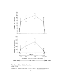 NUMBER OF INDIVIDUALS
NUMBER OF SPECIES
Cn-^
S&O-
^
OO\K —
b.
Ul
0.070-
0.125-
> 0471 —
— | u^ncn-
£ 0.658-
x 0785-
V> '°'
N
m
— * y '^c
^ <£.OOO
ro •* IAA
Ol-
K QQO
7 nKO
/ .UDU
o-
16.50
iQfin
23.0
44 n
""•*JOI-
o
5
1 1^ IO
— — ro ro oi en
en O en O 01 O en
OOOOOOOC
i i i i i i i
N
kD— 1
rw~i
KH
ho — 1 -
ho— 1
,1-gH ,
H G — |
1 x-> 1
(— e- 1
1 o _., J
1 o 1
r w 1
L - o J
h ^( "* I
f T r> ' 1
1 O 1
r ^^" n j
1 0 J
1 w 1
_ _ _ _ — iv> ro
^ro-t^cDODOro-^cDCDOro
i i i i i i i i i i i
KH
L -.^a - J
r ° 1
HH
HM
L r, 1
1 W" ' -|
MH
^^H
l__n J
1 ° 1
I 0 1
1 ° 1
L A J
1 'o 1 '
r ° 1
L ^r> 1
'l £ 1*
't—f^J° '
r-cH
L. .. -o 1
|" -O 1
L ^» '
1 o i
aMean and 95 percent confidence levels
bOrth 19775
Figure 12. Faunal characteristics of a Zpstera marina beda?
49
image:
NUMBER OF INDIVIDUALS
NUMBER OF SPECIES
Cn-^
S&O-
^
OO\K —
b.
Ul
0.070-
0.125-
> 0471 —
— | u^ncn-
£ 0.658-
x 0785-
V> '°'
N
m
— * y '^c
^ <£.OOO
ro •* IAA
Ol-
K QQO
7 nKO
/ .UDU
o-
16.50
iQfin
23.0
44 n
""•*JOI-
o
5
1 1^ IO
— — ro ro oi en
en O en O 01 O en
OOOOOOOC
i i i i i i i
N
kD— 1
rw~i
KH
ho — 1 -
ho— 1
,1-gH ,
H G — |
1 x-> 1
(— e- 1
1 o _., J
1 o 1
r w 1
L - o J
h ^( "* I
f T r> ' 1
1 O 1
r ^^" n j
1 0 J
1 w 1
_ _ _ _ — iv> ro
^ro-t^cDODOro-^cDCDOro
i i i i i i i i i i i
KH
L -.^a - J
r ° 1
HH
HM
L r, 1
1 W" ' -|
MH
^^H
l__n J
1 ° 1
I 0 1
1 ° 1
L A J
1 'o 1 '
r ° 1
L ^r> 1
'l £ 1*
't—f^J° '
r-cH
L. .. -o 1
|" -O 1
L ^» '
1 o i
aMean and 95 percent confidence levels
bOrth 19775
Figure 12. Faunal characteristics of a Zpstera marina beda?
49
image:
 to nothing by 1933 (see Table 7). The species still has not returned to this
area in marketable quantities. The life cycle of the bay scallop depends upon
the presence of eelgrass as a setting substrate for the post-veliger larvae
(Outsell 1930). Without this substrate, the scallop population would decline
rapidly since it completes its life cycle in two years.
Table 7. Harvested bay scallops (shucked meat), 1925-1975
Year Harvested Meat Value
(Kilograms) (dollars)
1925 5,050 74,272
1929 16,038 207,883
1930 25,549 147,564
1931 17,170 78,990
1932 9,220 80,090
1933 0 0
1975 0 0
Economic Uses and Problems
Eelgrass was apparently utilized in the past for a variety of different
economic reasons. Eelgrass had been used for fuel, mattress filling, packing,
upholstering, insulation, bedding for domestic animals, dike construction and
fertilizer (Burkholder and Doheny 1968; Cottam 1934tr, Phillips 1974a_). Its use
today is probably much more limited because of the development of alternative
synthetic substances. However, eelgrass is still used by some commercial fisher-
men in the Chesapeake Bay for packing soft shell crabs. Eelgrass can perhaps
be best used today as an organic mulch and compost for gardens.
The most important use of eelgrass today would be as an erosion control
barrier. Eelgrass, because of its abilities to reduce current and wave action
and bind sediments, could prove very effective as an alternative to bulkheading.
However, there have been no published attempts to establish eelgrass to stabi-
lize the shoreline. One would first have to establish the cost-effectiven ^s of
planting eelgrass or establishing a bulkhead prior to any attempts to initiate
this activity.
50
image:
to nothing by 1933 (see Table 7). The species still has not returned to this
area in marketable quantities. The life cycle of the bay scallop depends upon
the presence of eelgrass as a setting substrate for the post-veliger larvae
(Outsell 1930). Without this substrate, the scallop population would decline
rapidly since it completes its life cycle in two years.
Table 7. Harvested bay scallops (shucked meat), 1925-1975
Year Harvested Meat Value
(Kilograms) (dollars)
1925 5,050 74,272
1929 16,038 207,883
1930 25,549 147,564
1931 17,170 78,990
1932 9,220 80,090
1933 0 0
1975 0 0
Economic Uses and Problems
Eelgrass was apparently utilized in the past for a variety of different
economic reasons. Eelgrass had been used for fuel, mattress filling, packing,
upholstering, insulation, bedding for domestic animals, dike construction and
fertilizer (Burkholder and Doheny 1968; Cottam 1934tr, Phillips 1974a_). Its use
today is probably much more limited because of the development of alternative
synthetic substances. However, eelgrass is still used by some commercial fisher-
men in the Chesapeake Bay for packing soft shell crabs. Eelgrass can perhaps
be best used today as an organic mulch and compost for gardens.
The most important use of eelgrass today would be as an erosion control
barrier. Eelgrass, because of its abilities to reduce current and wave action
and bind sediments, could prove very effective as an alternative to bulkheading.
However, there have been no published attempts to establish eelgrass to stabi-
lize the shoreline. One would first have to establish the cost-effectiven ^s of
planting eelgrass or establishing a bulkhead prior to any attempts to initiate
this activity.
50
image:
 Some undesirable features of eel grass are hazards to small boats, hindrances
to navigation and interference with water skiing and swimming. On the Pacific
coast, eelgrass interfered with oyster harvesting and decreased amount of useable
bottom for oyster culture. Eelgrass was considered a nuisance and measures were
tried to eradicate it (Thomas 1967; Thomas and Duffy 1968).
Thus, today, there are very few direct uses of eelgrass. However, the in-
direct benefits to man, by supplying a food source to commercially important
species as the blue crab and sport fishes such as speckled and grey trout and
acting as a natural erosion control barrier, make this community very valuable
in the Bay.
Man's Impact on the Eelgrass Ecosystem
Because eelgrass inhabits the shallows of the coast zone, the increasing
use of this zone by man for industrial and recreational activities and the
coastal zone's susceptibility to point and non-point sources of pollution, make
this species extremely vulnerable to potential degradation.
Several examples from the Chesapeake Bay will illustrate these points.
Figure 13 shows an area of the south shore of the lower York River, Virginia,
taken in 1953 and 1960. The extent of the eelgrass bed is delineated in the
outlined area. The construction of an oil refinery and oil-generated power
plant in the seven years between the two photographs resulted in the extensive
loss of eelgrass, most likely resulting from construction activities (i.e.
increasing water turbidity) along the shore line. Today, there is no eelgrass
in front of the refinery or power plant. The loss of eelgrass was not natural
as eelgrass increased in area! extent directly across the river during
this same period. Recolonization of eelgrass after construction was finished
may have been prevented by alteration of sediments or perhaps the heated efflu-
ent from the power plant may have altered normal temperature patterns around
this area.
Figure 14 shows an area of the Severn River, a tributary of the Mobjack
Bay, Virginia. The light colored area surrounded by the darker band (eelgrass)
was the result of a dredging operation by a private individual for fill material.
This operation eliminated 1.3 ha of eelgrass. The speckled appearance of this
area is due to small patches of eelgrass and widgeongrass colonizing the area.
Figure 15 shows a portion of an eelgrass bed in the Mobjack Bay, Virginia.
The light bands crossing the eelgrass bed are the result of intense boating
activity in the grass area. This is not an atypical situation as many eelgrass
beds in the lower Bay, especially those in shallower areas, exhibit this criss-
crossing pattern.
Dredge and fill operations and spoil disposal pose a serious threat to
eelgrass survival. These activities alone can destroy or reduce eelgrass abun-
dance but the resultant activity usually increases the turbidity of a region
and this too may cause a decrease in eelgrass abundance, either through silting
and smothering or a reduction in light intensity below that necessary for photo-
synthetic maintenance.
51
image:
Some undesirable features of eel grass are hazards to small boats, hindrances
to navigation and interference with water skiing and swimming. On the Pacific
coast, eelgrass interfered with oyster harvesting and decreased amount of useable
bottom for oyster culture. Eelgrass was considered a nuisance and measures were
tried to eradicate it (Thomas 1967; Thomas and Duffy 1968).
Thus, today, there are very few direct uses of eelgrass. However, the in-
direct benefits to man, by supplying a food source to commercially important
species as the blue crab and sport fishes such as speckled and grey trout and
acting as a natural erosion control barrier, make this community very valuable
in the Bay.
Man's Impact on the Eelgrass Ecosystem
Because eelgrass inhabits the shallows of the coast zone, the increasing
use of this zone by man for industrial and recreational activities and the
coastal zone's susceptibility to point and non-point sources of pollution, make
this species extremely vulnerable to potential degradation.
Several examples from the Chesapeake Bay will illustrate these points.
Figure 13 shows an area of the south shore of the lower York River, Virginia,
taken in 1953 and 1960. The extent of the eelgrass bed is delineated in the
outlined area. The construction of an oil refinery and oil-generated power
plant in the seven years between the two photographs resulted in the extensive
loss of eelgrass, most likely resulting from construction activities (i.e.
increasing water turbidity) along the shore line. Today, there is no eelgrass
in front of the refinery or power plant. The loss of eelgrass was not natural
as eelgrass increased in area! extent directly across the river during
this same period. Recolonization of eelgrass after construction was finished
may have been prevented by alteration of sediments or perhaps the heated efflu-
ent from the power plant may have altered normal temperature patterns around
this area.
Figure 14 shows an area of the Severn River, a tributary of the Mobjack
Bay, Virginia. The light colored area surrounded by the darker band (eelgrass)
was the result of a dredging operation by a private individual for fill material.
This operation eliminated 1.3 ha of eelgrass. The speckled appearance of this
area is due to small patches of eelgrass and widgeongrass colonizing the area.
Figure 15 shows a portion of an eelgrass bed in the Mobjack Bay, Virginia.
The light bands crossing the eelgrass bed are the result of intense boating
activity in the grass area. This is not an atypical situation as many eelgrass
beds in the lower Bay, especially those in shallower areas, exhibit this criss-
crossing pattern.
Dredge and fill operations and spoil disposal pose a serious threat to
eelgrass survival. These activities alone can destroy or reduce eelgrass abun-
dance but the resultant activity usually increases the turbidity of a region
and this too may cause a decrease in eelgrass abundance, either through silting
and smothering or a reduction in light intensity below that necessary for photo-
synthetic maintenance.
51
image:
 <T3
4-
O
o
3
-p
co
o
o
Ol
_c
-M
s_
0)
4J
4-
rc
CO
(O
O)
S-
re
HI
to
CO
(O
i.
CT
"ol
O)
to
to
O
O)
u
c
(1)
T3
O) i-
c o
•I- +J <4-
O <o to
to Q. C
to S- O
<— ni o
Q- 3
(COO)
S- CL O
O) C
O "O 0)
4J C S-
O fO CV
i— CD
(O
2
(C
O
vo
ro
in
(T3
Dl
1.
S.
(U
•r-
o:
o
o
0)
D>
52
image:
<T3
4-
O
o
3
-p
co
o
o
Ol
_c
-M
s_
0)
4J
4-
rc
CO
(O
O)
S-
re
HI
to
CO
(O
i.
CT
"ol
O)
to
to
O
O)
u
c
(1)
T3
O) i-
c o
•I- +J <4-
O <o to
to Q. C
to S- O
<— ni o
Q- 3
(COO)
S- CL O
O) C
O "O 0)
4J C S-
O fO CV
i— CD
(O
2
(C
O
vo
ro
in
(T3
Dl
1.
S.
(U
•r-
o:
o
o
0)
D>
52
image:
 The light colored area in the middle of the eel grass bed was the result of
dredging activities in this area for fill material for the adjacent marsh.
Figure 14. Aerial photograph of an area in the Severn River, Virginia3
53
image:
The light colored area in the middle of the eel grass bed was the result of
dredging activities in this area for fill material for the adjacent marsh.
Figure 14. Aerial photograph of an area in the Severn River, Virginia3
53
image:
 Light colored streaks across the eelgrass bed are boat tracks
Figure 15.
Virginia9
Aerial photograph of a portion of an eelgrass bed in Mobjack Bay,
54
image:
Light colored streaks across the eelgrass bed are boat tracks
Figure 15.
Virginia9
Aerial photograph of a portion of an eelgrass bed in Mobjack Bay,
54
image:
 The activities mentioned above in the Chesapeake Bay are not unique to
this area. The increasing demand for waterfront property with deep water piers
and recreational pressure in the shallows make it imperative for the development
of some management scheme for the protection of eel grass.
Causes for the Decline of Eel grass in the Chesapeake Bay. Eel grass in the
past has undergone major fluctutations in abundance, the most well-documented
being the one that occurred in the 1930s along the East Coast of the U.S. and
the West Coast of Europe. The cause for this decline was attributed to a pro-
tozoan, Labyrinthula (Renn 1934, 1935, 1937) though many other causes were sug-
gested (e.g. salinity, climatical changes, pollution). That Labyrinthula was
the sole cause for this decline has not been proven conclusively and recent
papers (Rasmussen 1973, 1977) cite this as a secondary agent because Labyrinthula
has been found living on healthy eel grass instead of being only on dead eel grass.
More recently, temperature has been implicated as the major factor for
causing changes in eelgrass abundance (McRoy 1966; Rasmussen 1973, 1977; Orth
1976). Temperature is extremely important in regulating the growth, reproduc-
tion and senescense of eelgrass and it is not an unreasonable assumption to
implicate temperature as a primary agent in the decline of eelgrass.
Rasmussen (1973, 1977) examined patterns of abundance of eelgrass in Denmark
and correlated this with annual temperature patterns. He attributed eelgrass
fluctuations to warm summers and exceptionally mild winters. He postulated that
high water temperature would weaken the plant, which directly affected metabolism
and indrectly weakened the plant making it more susceptible to the ever-present
bacteria and protozoa.
The first recently recorded decline of the major eelgrass beds in the Bay
occurred in the early fall, 1973, and another mass defoliation in the early fall
of 1975. Some eelgrass areas, for example in Mobjack Bay, did not decline dur-
ing 1973 but declined in 1975. There were reports of declines of eelgrass in
1972 after Agnes but these were limited to the up-estuary limits of eelgrass.
It appears that the freshet produced by Agnes did not cause the decline unless
there was a delayed reaction which did not appear until a year later. This
appears unreasonable since eelgrass declined almost 14 months after Agnes.
The period of the early to mid 1970s was marked by a warming trend charac-
terized by warm winters (see Figure 16). Because eelgrass is approaching its
southern limits in the Chesapeake Bay (North Carolina is the southern limit of
eelgrass on the East Coast) any shift in the critical temperature regime may
dramatically affect the growth cycle of eelgrass. There is no documented evi-
dence from North Carolina to indicate recent changes in abundance of eelgrass
aside from small areas. However, Dillon (1971) found the almost complete die-
off of eelgrass in the late summer with subsequent regrowth from seedlings and
rhizomes. Whether this phenomenon observed in North Carolina is an annual
occurrence is unknown, but this was similar to what had happended in the Bay,
except that in many areas, e.g. the York River and the Rappahannock River,
there has been very little regrowth.
There have been no reports of eelgrass die-backs north of Chesapeake Bay
to Maine but there have been no extensive surveys of eelgrass populations in
55
image:
The activities mentioned above in the Chesapeake Bay are not unique to
this area. The increasing demand for waterfront property with deep water piers
and recreational pressure in the shallows make it imperative for the development
of some management scheme for the protection of eel grass.
Causes for the Decline of Eel grass in the Chesapeake Bay. Eel grass in the
past has undergone major fluctutations in abundance, the most well-documented
being the one that occurred in the 1930s along the East Coast of the U.S. and
the West Coast of Europe. The cause for this decline was attributed to a pro-
tozoan, Labyrinthula (Renn 1934, 1935, 1937) though many other causes were sug-
gested (e.g. salinity, climatical changes, pollution). That Labyrinthula was
the sole cause for this decline has not been proven conclusively and recent
papers (Rasmussen 1973, 1977) cite this as a secondary agent because Labyrinthula
has been found living on healthy eel grass instead of being only on dead eel grass.
More recently, temperature has been implicated as the major factor for
causing changes in eelgrass abundance (McRoy 1966; Rasmussen 1973, 1977; Orth
1976). Temperature is extremely important in regulating the growth, reproduc-
tion and senescense of eelgrass and it is not an unreasonable assumption to
implicate temperature as a primary agent in the decline of eelgrass.
Rasmussen (1973, 1977) examined patterns of abundance of eelgrass in Denmark
and correlated this with annual temperature patterns. He attributed eelgrass
fluctuations to warm summers and exceptionally mild winters. He postulated that
high water temperature would weaken the plant, which directly affected metabolism
and indrectly weakened the plant making it more susceptible to the ever-present
bacteria and protozoa.
The first recently recorded decline of the major eelgrass beds in the Bay
occurred in the early fall, 1973, and another mass defoliation in the early fall
of 1975. Some eelgrass areas, for example in Mobjack Bay, did not decline dur-
ing 1973 but declined in 1975. There were reports of declines of eelgrass in
1972 after Agnes but these were limited to the up-estuary limits of eelgrass.
It appears that the freshet produced by Agnes did not cause the decline unless
there was a delayed reaction which did not appear until a year later. This
appears unreasonable since eelgrass declined almost 14 months after Agnes.
The period of the early to mid 1970s was marked by a warming trend charac-
terized by warm winters (see Figure 16). Because eelgrass is approaching its
southern limits in the Chesapeake Bay (North Carolina is the southern limit of
eelgrass on the East Coast) any shift in the critical temperature regime may
dramatically affect the growth cycle of eelgrass. There is no documented evi-
dence from North Carolina to indicate recent changes in abundance of eelgrass
aside from small areas. However, Dillon (1971) found the almost complete die-
off of eelgrass in the late summer with subsequent regrowth from seedlings and
rhizomes. Whether this phenomenon observed in North Carolina is an annual
occurrence is unknown, but this was similar to what had happended in the Bay,
except that in many areas, e.g. the York River and the Rappahannock River,
there has been very little regrowth.
There have been no reports of eelgrass die-backs north of Chesapeake Bay
to Maine but there have been no extensive surveys of eelgrass populations in
55
image:
 UJ
Lt
cc.
U
O.
ft
UJ
20
15
0
20
10
0
20
10
0
20
0
30
20
10
0
30
20
10
0
30
20
10
0
SUMMER
BOSTON, *&«$.
NEW YORK (ftotttf?)
, MO.
SOLOMONS ISLAND, MO,
GLOUCESTER POINT, VA.
'" |""l""l""l""l""l""l""l""l ""I""!""!""!""!""!
1910 1920 1930 1940 1950 I960 1970 I960
Figure 16. Mean temperatures for coldest
and warmest months at various East Coast
locations, 1906-1977
56
image:
UJ
Lt
cc.
U
O.
ft
UJ
20
15
0
20
10
0
20
10
0
20
0
30
20
10
0
30
20
10
0
30
20
10
0
SUMMER
BOSTON, *&«$.
NEW YORK (ftotttf?)
, MO.
SOLOMONS ISLAND, MO,
GLOUCESTER POINT, VA.
'" |""l""l""l""l""l""l""l""l ""I""!""!""!""!""!
1910 1920 1930 1940 1950 I960 1970 I960
Figure 16. Mean temperatures for coldest
and warmest months at various East Coast
locations, 1906-1977
56
image:
 these areas, as have been done in the Bay. An examination of temperature
records for various locations along the East Coast (see Figure 16) also indicate
a warming trend in the 1970s but with no apparent decline of eel grass.
The temperature records for the East Coast showed a warm period (i.e. warm
winters) around 1932 (see Figure 16). The winter of 1932 was unusual because
the coldest month was March contrasted to January and February in other years.
This period was also preceded by a decade of stable cold winters. If the hypo-
thesis that extreme temperature conditions stress the plants is correct, then
extreme variations in certain temperature patterns may account for the eel grass
decline in the 1930s. However, the picture is confused by another warming period
in the early 1950s when, supposedly, eel grass was exhibiting an upswing in abun-
dance. Eel grass was abundant in 1953 in the lower York River, Virginia, but it
is not known what preceded this period in terms of eel grass coverage. Also
lacking are precise data as to rate of recovery and any seasonal changes in
already existing beds during periods of recovery.
Temperature may be the primary cause for the disappearance of eel grass but
the lack of controlled experiments over extended periods along with accurate
information of present status of existing eel grass, makes this only an hypothesis
for the disappearance of eel grass.
POTAMOGETON PECTINATUS
Biology
General Morphology. In its native setting, Potamogeton pectinatus, or
sago pondweed, is completely submerged and recognized by a characteristic fan!ike
spreading of leaves at the water's surface (see Figure 17). P_. pectinatus
derives its name from the pectinate or closely inserted growth of its stems and
leaves. The stems often develop up to 2 to 5 m in length and support linear-
filiform leaf blades 5 to 35 cm long. Leaf tips are sharply pointed to gradually
tapered in young plants. With increasing age, several types of leaf ends can
occur on the same plant (Mason 1969).
Two morphological forms of reproductive structures include leafy outgrowths
or auxiliary tubers and slender peduncles. The peduncles, ranging in length
from 50 to 25 cm, have spikes conspicuously interrupted by 2 to 6 whorls, with
the axis of the spike becoming lax at maturity (Mason 1969). The starch con-
taining druplets of this species can be distinguished from other pondweeds by
the rounded apex of the trap door (Martin and Uhler 1939). The rootstocks are
long and straight and often bear rhizoids or specialized turions or winter buds
rich in starch (Hotchkiss 1967; Sculthorpe 1967).
There is a reduction series in the general anatomy of Potamogetonaceae
with P_. pectinatus illustrating the most simplistic and reduce form. Unlike
other species, the stem of P_. pectinatus displays a homogeneous zone of phloem
surrounding the axial lacuna (Sculthorpe 1967). In the roots the xylem is a
single central vessel with the five protoxylem elements absent at maturity
(Arbor 1920).
57
image:
these areas, as have been done in the Bay. An examination of temperature
records for various locations along the East Coast (see Figure 16) also indicate
a warming trend in the 1970s but with no apparent decline of eel grass.
The temperature records for the East Coast showed a warm period (i.e. warm
winters) around 1932 (see Figure 16). The winter of 1932 was unusual because
the coldest month was March contrasted to January and February in other years.
This period was also preceded by a decade of stable cold winters. If the hypo-
thesis that extreme temperature conditions stress the plants is correct, then
extreme variations in certain temperature patterns may account for the eel grass
decline in the 1930s. However, the picture is confused by another warming period
in the early 1950s when, supposedly, eel grass was exhibiting an upswing in abun-
dance. Eel grass was abundant in 1953 in the lower York River, Virginia, but it
is not known what preceded this period in terms of eel grass coverage. Also
lacking are precise data as to rate of recovery and any seasonal changes in
already existing beds during periods of recovery.
Temperature may be the primary cause for the disappearance of eel grass but
the lack of controlled experiments over extended periods along with accurate
information of present status of existing eel grass, makes this only an hypothesis
for the disappearance of eel grass.
POTAMOGETON PECTINATUS
Biology
General Morphology. In its native setting, Potamogeton pectinatus, or
sago pondweed, is completely submerged and recognized by a characteristic fan!ike
spreading of leaves at the water's surface (see Figure 17). P_. pectinatus
derives its name from the pectinate or closely inserted growth of its stems and
leaves. The stems often develop up to 2 to 5 m in length and support linear-
filiform leaf blades 5 to 35 cm long. Leaf tips are sharply pointed to gradually
tapered in young plants. With increasing age, several types of leaf ends can
occur on the same plant (Mason 1969).
Two morphological forms of reproductive structures include leafy outgrowths
or auxiliary tubers and slender peduncles. The peduncles, ranging in length
from 50 to 25 cm, have spikes conspicuously interrupted by 2 to 6 whorls, with
the axis of the spike becoming lax at maturity (Mason 1969). The starch con-
taining druplets of this species can be distinguished from other pondweeds by
the rounded apex of the trap door (Martin and Uhler 1939). The rootstocks are
long and straight and often bear rhizoids or specialized turions or winter buds
rich in starch (Hotchkiss 1967; Sculthorpe 1967).
There is a reduction series in the general anatomy of Potamogetonaceae
with P_. pectinatus illustrating the most simplistic and reduce form. Unlike
other species, the stem of P_. pectinatus displays a homogeneous zone of phloem
surrounding the axial lacuna (Sculthorpe 1967). In the roots the xylem is a
single central vessel with the five protoxylem elements absent at maturity
(Arbor 1920).
57
image:
 (copied from Hotchkiss 1967)
Figure 17. Sago pondweed (fotamogeton pectinatus)
58
image:
(copied from Hotchkiss 1967)
Figure 17. Sago pondweed (fotamogeton pectinatus)
58
image:
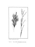 Reproduction. Potamogeton pectinatus reproduces both sexually and
asexually. Sexual reproduction occurs through the production of monoecious
flowers arranged in a spike (Yeo 1965aJ. In a series of studies on reproduc-
tion in an irrigation ditch in Huntley, Montana, Yeo (1965a) determined that
pollination, fertilization and fruit development occur at the water/air inter-
face. Pollen floats on the surface (Sculthorpe 1967) and after fertilization
a druplet is formed. These seeds remain on the rachis of the inflorescence
until late fall or until they are removed by moving water (Yeo 1965a_).
Vegetative reproduction occurs by two separate mechanisms to form propa-
gules. Subterranean tubers develop from specialized tissue at the branch ends.
Occuring in chains of up to five tubers, these structures store large amounts of
starch and persist over winter to produce shoots the following spring. A second
mode of vegetative reproduction occurs through the development of axillary tubers
which form in the fall from the ends of leaf shoots in the leaf axils. Similar
to the subterranean tubers, these axillary structures occur singly or in pairs,
sink to the bottom and form new plants in the spring (Yeo 1965a).
Based on single season experiments using different sized pools, Yeo (1965bJ
found that the number of tubers and seeds produced from plants grown from tubers
increased as pool sizes increased. In the largest pool (about 23.6 m2), one sago
pondweed plant developed over 36,000 subterranean tubers, 800 axillary tubers
and 6,000 seeds within six months. Yeo's experiments readily demonstrated the
rapidity with which sago pondweed can colonize a favorable habitat within a
short period of time.
Distribution
Potamogeton pectinatus is reported in similar habitats all over the world.
Not only does the range of this perennial include fresh streams and ponds, but
also brackish coastal waters of the United States and portions of Canada. It
has been observed in Russia, India, South Africa, Hungary, Pakistan, and East
Germany and exhibits a wide range in altitude from sea level in England to about
5,000 m in Venezuela and Tibet (Klokov and Zimbalevskaya 1974; Misra 1972; Hill
et al. 1975; Andrikovics 1973; Ali 1973; Krausch 1976; Ascherson and Grabener
1907.
Though most abundant in the northwestern states and the Chesapeake Bay in
the United States (Martin and Uhler 1939), it is reported to be a pest species
often encountered in the operation of irrigation systems in the west (Hodgson
and Otto 1963) and in water supply ditches in the cranberry bogs of Massachusetts
(Devlin 1973).
The continuing survey of submerged aquatic vegetation that is being con-
ducted annually by MBHRL has documented P. pectinatus in the Chesapeake from
1971 to 1977 with the exception of 1975 Tsee Table 8 and Figure 18). Results
of the summer survey for 1977 are not available at this time for the individual
species. The 1972 sampling yielded the highest percentage of vegetated stations
despite the fact that sampling was conducted subsequent to Hurricane Agnes. MBHRL
survey crews found sago pondweed at 5.69 percent of the 615 stations sampled in
1972 from the Chester River south into Tangier Sound on the Eastern Shore and in
the Severn and Patapsco Rivers on the Western Shore. In 1973, P_. pectinatus
59
image:
Reproduction. Potamogeton pectinatus reproduces both sexually and
asexually. Sexual reproduction occurs through the production of monoecious
flowers arranged in a spike (Yeo 1965aJ. In a series of studies on reproduc-
tion in an irrigation ditch in Huntley, Montana, Yeo (1965a) determined that
pollination, fertilization and fruit development occur at the water/air inter-
face. Pollen floats on the surface (Sculthorpe 1967) and after fertilization
a druplet is formed. These seeds remain on the rachis of the inflorescence
until late fall or until they are removed by moving water (Yeo 1965a_).
Vegetative reproduction occurs by two separate mechanisms to form propa-
gules. Subterranean tubers develop from specialized tissue at the branch ends.
Occuring in chains of up to five tubers, these structures store large amounts of
starch and persist over winter to produce shoots the following spring. A second
mode of vegetative reproduction occurs through the development of axillary tubers
which form in the fall from the ends of leaf shoots in the leaf axils. Similar
to the subterranean tubers, these axillary structures occur singly or in pairs,
sink to the bottom and form new plants in the spring (Yeo 1965a).
Based on single season experiments using different sized pools, Yeo (1965bJ
found that the number of tubers and seeds produced from plants grown from tubers
increased as pool sizes increased. In the largest pool (about 23.6 m2), one sago
pondweed plant developed over 36,000 subterranean tubers, 800 axillary tubers
and 6,000 seeds within six months. Yeo's experiments readily demonstrated the
rapidity with which sago pondweed can colonize a favorable habitat within a
short period of time.
Distribution
Potamogeton pectinatus is reported in similar habitats all over the world.
Not only does the range of this perennial include fresh streams and ponds, but
also brackish coastal waters of the United States and portions of Canada. It
has been observed in Russia, India, South Africa, Hungary, Pakistan, and East
Germany and exhibits a wide range in altitude from sea level in England to about
5,000 m in Venezuela and Tibet (Klokov and Zimbalevskaya 1974; Misra 1972; Hill
et al. 1975; Andrikovics 1973; Ali 1973; Krausch 1976; Ascherson and Grabener
1907.
Though most abundant in the northwestern states and the Chesapeake Bay in
the United States (Martin and Uhler 1939), it is reported to be a pest species
often encountered in the operation of irrigation systems in the west (Hodgson
and Otto 1963) and in water supply ditches in the cranberry bogs of Massachusetts
(Devlin 1973).
The continuing survey of submerged aquatic vegetation that is being con-
ducted annually by MBHRL has documented P. pectinatus in the Chesapeake from
1971 to 1977 with the exception of 1975 Tsee Table 8 and Figure 18). Results
of the summer survey for 1977 are not available at this time for the individual
species. The 1972 sampling yielded the highest percentage of vegetated stations
despite the fact that sampling was conducted subsequent to Hurricane Agnes. MBHRL
survey crews found sago pondweed at 5.69 percent of the 615 stations sampled in
1972 from the Chester River south into Tangier Sound on the Eastern Shore and in
the Severn and Patapsco Rivers on the Western Shore. In 1973, P_. pectinatus
59
image:
 Table 8. Percent of sampling stations showing occurrence of
Potamogeton pectinatus, Maryland Chesapeake Bay, 1971-19763
Area
Code
1
2
3
4
5
6
7
8
9
10
11
12
13
14
15
16
17
18
19
20
21
22
23
24
25
26
Number
River system
Elk & Bohemia
Rivers
Sassafras River
Howe 11 & Swan
Points
Eastern Bay
Choptank River
Little Choptank
River
James Island *
Honga River
Honga River
Bloodsworth Is.
Susquehanna
Flats
Fishing Bay
Nantiocke &
Wicomico Rivers
Hanokin River
Patapsco River
Big & Little
Annemessex Rivers
Gunpowder & Bush
River Headwaters
Pocomoke Sound
(Maryland)
Magothy River
Severn River
Patuxent River
Back, Middle &
Gunpowder Rivers
Curtis & Cove
Points
South, West &
Rhode Rivers
Chester River
Love & Kent
Points
Smith Island
(Maryland)
Total
1971
0
0
0
0
1.67
5.26
0
0
2.50
0
0
0
0
0
5.00
0
0
16.67
0
0
0
0
0
5.56
0
0
1.28
1972
0
0
0
9.30
3.45
10.53
20.59
10.00
6.82
0
0
0
13.33
5.00
25.00
0
0
0
13.33
0
0
0
0
2.78
0
27.27
5.69
1973
0
0
0
6.38
7.02
0
0
3.33
6.52
0
0
0
0
0
5.00
0
0
8.33
13.33
0
0
0
0
5.88
0
8.33
2.86
1974
0
0
0
2.13
0
0
0
0
0
0
0
0
0
0
0
0
-
0
13.33
0
0
0
0
14.71
0
0
1.31
1975
0
0
0
0
0
0
0
0
0
0
0
0
0
0
0
-
0
-
-
0
0
0
0
0
0
0
0
1976
0
0
0
2.22
0
0
0
0
0
0
0
0
0
0
0
0
0
0
0
0
0
0
0
5.71
0
0
0.48
71
15
10
12
47
60
19
34
30
40
27
25
30
15
21
20
9
22
12
15
50
22
20
8
36
8
17
624
72
16
10
6
43
58
19
34
30
44
37
25
30
15
20
20
8
20
12
15
47
22
19
10
36
8
11
615
of
/3
16
10
12
47
57
19
34
30
46
37
25
30
15
21
20
7
21
12
15
50
22
19
10
34
8
12
629
stations
74
16
10
12
47
58
19
34
30
43
37
25
30
15
21
19
9
-
12
15
50
22
19
8
34
8
17
610
75
16
10
12
46
57
19
34
29
43
36
24
30
14
-
18
-
20
-
-
47
22
6
8
36
8
17
553
76
16
10
12
45
56
19
34
29
45
35
25
30
15
21
20
9
22
12
13
49
22
21
8
35
8
17
628
U.S. Fish and Wildlife Service Migratory Bird and Habitat Research Laboratory, 1976
60
image:
Table 8. Percent of sampling stations showing occurrence of
Potamogeton pectinatus, Maryland Chesapeake Bay, 1971-19763
Area
Code
1
2
3
4
5
6
7
8
9
10
11
12
13
14
15
16
17
18
19
20
21
22
23
24
25
26
Number
River system
Elk & Bohemia
Rivers
Sassafras River
Howe 11 & Swan
Points
Eastern Bay
Choptank River
Little Choptank
River
James Island *
Honga River
Honga River
Bloodsworth Is.
Susquehanna
Flats
Fishing Bay
Nantiocke &
Wicomico Rivers
Hanokin River
Patapsco River
Big & Little
Annemessex Rivers
Gunpowder & Bush
River Headwaters
Pocomoke Sound
(Maryland)
Magothy River
Severn River
Patuxent River
Back, Middle &
Gunpowder Rivers
Curtis & Cove
Points
South, West &
Rhode Rivers
Chester River
Love & Kent
Points
Smith Island
(Maryland)
Total
1971
0
0
0
0
1.67
5.26
0
0
2.50
0
0
0
0
0
5.00
0
0
16.67
0
0
0
0
0
5.56
0
0
1.28
1972
0
0
0
9.30
3.45
10.53
20.59
10.00
6.82
0
0
0
13.33
5.00
25.00
0
0
0
13.33
0
0
0
0
2.78
0
27.27
5.69
1973
0
0
0
6.38
7.02
0
0
3.33
6.52
0
0
0
0
0
5.00
0
0
8.33
13.33
0
0
0
0
5.88
0
8.33
2.86
1974
0
0
0
2.13
0
0
0
0
0
0
0
0
0
0
0
0
-
0
13.33
0
0
0
0
14.71
0
0
1.31
1975
0
0
0
0
0
0
0
0
0
0
0
0
0
0
0
-
0
-
-
0
0
0
0
0
0
0
0
1976
0
0
0
2.22
0
0
0
0
0
0
0
0
0
0
0
0
0
0
0
0
0
0
0
5.71
0
0
0.48
71
15
10
12
47
60
19
34
30
40
27
25
30
15
21
20
9
22
12
15
50
22
20
8
36
8
17
624
72
16
10
6
43
58
19
34
30
44
37
25
30
15
20
20
8
20
12
15
47
22
19
10
36
8
11
615
of
/3
16
10
12
47
57
19
34
30
46
37
25
30
15
21
20
7
21
12
15
50
22
19
10
34
8
12
629
stations
74
16
10
12
47
58
19
34
30
43
37
25
30
15
21
19
9
-
12
15
50
22
19
8
34
8
17
610
75
16
10
12
46
57
19
34
29
43
36
24
30
14
-
18
-
20
-
-
47
22
6
8
36
8
17
553
76
16
10
12
45
56
19
34
29
45
35
25
30
15
21
20
9
22
12
13
49
22
21
8
35
8
17
628
U.S. Fish and Wildlife Service Migratory Bird and Habitat Research Laboratory, 1976
60
image:
 1971
1973
1975
1972
1974
1976
Figure 18. Distribution of Potamogeton pectinatus, Maryland Chesapeake
Bay, 1971-1976
61
image:
1971
1973
1975
1972
1974
1976
Figure 18. Distribution of Potamogeton pectinatus, Maryland Chesapeake
Bay, 1971-1976
61
image:
 was found in the same general areas but at only 2.86 of the 629 stations sampled
In 1974 this species was found in only three river systems compared to 12 in
1972. In 1975 no IP. pectinatus was found at any of the 553 stations sampled.
By 1976 only Eastern Bay and Chester River showed any sago pondweed.
Environmental Factors Affecting Distribution
Temperature. Temperature often determines the type of vegetation produced
and limits its distribution. In English lakes, Pearsall (1920) reported that
growth of IP. pectinatus did not occur until mid-June (mean temperature 12.3 C)
even though maximum sunshine had persisted since May. Yeo (1965b) stated that
_P. pectinatus propagules planted in water temperatures of 13 C did not germinate;
however, those planted later in the season when temperatures reached 15 to 18 C
did germinate.
Salinity. Teeter (1965) discussed work by Metcalf (1931) documenting sago
pondweed in North Dakota. Through his own research, Teeter was not able to cor-
roborate Metcalf's high salinity tolerance level but did provide data relating
salinity to seed production, set and germination plus tuber growth and production.
In general, Teeter observed that growing, healthy plants could tolerate salinity
levels that killed mature plants which had slower growth rates. Maximum seed
production, seed germination and vegetative growth occurred in freshwater.
Salinities of 8 to 9 ppt generally decreased growth and germination rates by 50
percent. Salinity at 3 ppt stimulated tuber production and growth.
Substrate. According to Sculthorpe (1967), P. pectinatus is a "silt-
loving" species. A study by Hannan (1967), concluded that plants (including
P_. pectinatus) in gravel and mud-gravel transition beds had shorter shoots than
plants growing in mud and silt-pebble beds. The latter displayed continuous
growth and an increase in species number. Rickett (1923) reported that
P_. pectinatus grew on both mud and sand bottoms.
Light, Depth and Turbidity. Bourn (1932), in studying Back Bay and
Currituck Sound, determined that JP. pectinatus required at least 3.5 percent
total sunlight for growth. Much below 4.0 percent total solar energy, growth
declined rapidly. Based on Bourn's field observations, it appeared that sub-
terranean tuber size and quantity decreased with decreasing light. Shading of
P_. pectinatus plants produced yellowed, sparse foliage, elongated nodes and
rigid unbranched stems. Stem tips and terminal leaves protruded above the
water surface and wilted.
Current, Hind and Wave Action. Under conditions of strong winds and wave
action, P_. pectinatus can persist due to a lattice root structure (Hannan 1967).
This may have been instrumental in sago pondweed's persistence in the Chesapeake
Bay through Hurricane Agnes in June 1972. Even though the species has recent-
ly declined subsequent to the hurricane, the July 1972 sampling of the Bay by
MBHRL showed the highest percent of P_. pectinatus occurrence of the six-year
survey.
62
image:
was found in the same general areas but at only 2.86 of the 629 stations sampled
In 1974 this species was found in only three river systems compared to 12 in
1972. In 1975 no IP. pectinatus was found at any of the 553 stations sampled.
By 1976 only Eastern Bay and Chester River showed any sago pondweed.
Environmental Factors Affecting Distribution
Temperature. Temperature often determines the type of vegetation produced
and limits its distribution. In English lakes, Pearsall (1920) reported that
growth of IP. pectinatus did not occur until mid-June (mean temperature 12.3 C)
even though maximum sunshine had persisted since May. Yeo (1965b) stated that
_P. pectinatus propagules planted in water temperatures of 13 C did not germinate;
however, those planted later in the season when temperatures reached 15 to 18 C
did germinate.
Salinity. Teeter (1965) discussed work by Metcalf (1931) documenting sago
pondweed in North Dakota. Through his own research, Teeter was not able to cor-
roborate Metcalf's high salinity tolerance level but did provide data relating
salinity to seed production, set and germination plus tuber growth and production.
In general, Teeter observed that growing, healthy plants could tolerate salinity
levels that killed mature plants which had slower growth rates. Maximum seed
production, seed germination and vegetative growth occurred in freshwater.
Salinities of 8 to 9 ppt generally decreased growth and germination rates by 50
percent. Salinity at 3 ppt stimulated tuber production and growth.
Substrate. According to Sculthorpe (1967), P. pectinatus is a "silt-
loving" species. A study by Hannan (1967), concluded that plants (including
P_. pectinatus) in gravel and mud-gravel transition beds had shorter shoots than
plants growing in mud and silt-pebble beds. The latter displayed continuous
growth and an increase in species number. Rickett (1923) reported that
P_. pectinatus grew on both mud and sand bottoms.
Light, Depth and Turbidity. Bourn (1932), in studying Back Bay and
Currituck Sound, determined that JP. pectinatus required at least 3.5 percent
total sunlight for growth. Much below 4.0 percent total solar energy, growth
declined rapidly. Based on Bourn's field observations, it appeared that sub-
terranean tuber size and quantity decreased with decreasing light. Shading of
P_. pectinatus plants produced yellowed, sparse foliage, elongated nodes and
rigid unbranched stems. Stem tips and terminal leaves protruded above the
water surface and wilted.
Current, Hind and Wave Action. Under conditions of strong winds and wave
action, P_. pectinatus can persist due to a lattice root structure (Hannan 1967).
This may have been instrumental in sago pondweed's persistence in the Chesapeake
Bay through Hurricane Agnes in June 1972. Even though the species has recent-
ly declined subsequent to the hurricane, the July 1972 sampling of the Bay by
MBHRL showed the highest percent of P_. pectinatus occurrence of the six-year
survey.
62
image:
 Sedimentation. Sago pondweed has long, narrow, vertical leaves which do
not provide a good surface for settling particles or organisms. This allows
for participate matter to settle and build up bottom sediments more conducive
to invasion by other macrophytes (Butcher 1933).
Nutrient Response. Sculthorpe (1967) listed P_. pectinatus as capable of
tolerating river water polluted with sewage, other wastes and high nutrient
levels that tend to limit other species. Jones and Cullimore (1973) correlated
a wide range of nutrient levels in Canadian lakes with the distribution of
vegetation. In all cases studied, P_. pectinatus was a predominant species in
the lakes. These studies were undertaken in late May and early June during a
time when nutrient levels were critical to the development of young plants. The
nutrient ranges supporting the largest populations of P_. pectinatus included:
Nitrates 0.13 to 1.7 ppm
TKN 1.14 to 1.8 ppm
Total phosphate (dissolved) 0.6 to 1.7 ppm
Total inorganic carbon 28 to 42 ppm
Total hardness (CaCo3) 346 to 405 ppm
Total organic carbon 12 to 18 ppm
Total phosphate (sediment) 0.03 to 2 ppm
Susceptibility. Heavy metals and herbicides are selectively toxic to
P_. pectinatus plants. Analysis of plant ash contents have revealed that these
plants can concentrate high levels of vanadium (16,500 ppm) and lower levels of
cobalt and nickel (2.8 ppm and 12 ppm respectively) (Varenko and Chuiko 1971).
Plants exposed to 0.12 ppm copper in the form of copper sulfate penthydrate
resulted in the development of proportionally shorter stems with yellowing of
plant tissue. In the case of acute copper toxicity, the plant's outer surface
became brown and internodes were shorter giving the plant a rosette appearance
(Ryan and Riemer 1975).
Selectively researched herbicides, commonly used for the control of
terrestrial weeds, have been reported by Yeo (1966) to be toxic to P_. pectinatus.
Experiments indicated that popularly used diquat and paraquat controlled the
growth of sago pondweed. Application rates of 250 ppb of diquat or paraquat
controlled plant growth for eight weeks. A concentration of 125 ppb diquat con-
trolled plant growth in two reservoirs but was unsuccessful in two others.
Experiments by Frank et al. (1963) found that Potamogeton spp. were satis-
factorily controlled by atrazine granules applied at 5 and 6 ppm a.i.. Simazine
applied at 4.5 to 9 kg/ha controlled the growth of Potamogeton spp.
Newbold (1975) indicated that P_. pectinatus was controlled in a pond for a
year by concentrations of 10, 20 or 40 mg/1 dichlobenil and chlorthiamid. A
comparatively low concentration of 0.05 mg/1 terbutryne controlled growth for
one year. A concentration of 2 ppm a.i. silvex and 7 to 10 ppm a.i. sodium
arsenite have been recorded to cause the cessation of IP. pectinatus growth
(Lawrence and Hollingsworth 1969).
Experiments by Devlin et al. (1972) and Devlin and Karczmarczyk (1975)
on the effects of napthalam and norflurazon on sago pondweed, suggested that
63
image:
Sedimentation. Sago pondweed has long, narrow, vertical leaves which do
not provide a good surface for settling particles or organisms. This allows
for participate matter to settle and build up bottom sediments more conducive
to invasion by other macrophytes (Butcher 1933).
Nutrient Response. Sculthorpe (1967) listed P_. pectinatus as capable of
tolerating river water polluted with sewage, other wastes and high nutrient
levels that tend to limit other species. Jones and Cullimore (1973) correlated
a wide range of nutrient levels in Canadian lakes with the distribution of
vegetation. In all cases studied, P_. pectinatus was a predominant species in
the lakes. These studies were undertaken in late May and early June during a
time when nutrient levels were critical to the development of young plants. The
nutrient ranges supporting the largest populations of P_. pectinatus included:
Nitrates 0.13 to 1.7 ppm
TKN 1.14 to 1.8 ppm
Total phosphate (dissolved) 0.6 to 1.7 ppm
Total inorganic carbon 28 to 42 ppm
Total hardness (CaCo3) 346 to 405 ppm
Total organic carbon 12 to 18 ppm
Total phosphate (sediment) 0.03 to 2 ppm
Susceptibility. Heavy metals and herbicides are selectively toxic to
P_. pectinatus plants. Analysis of plant ash contents have revealed that these
plants can concentrate high levels of vanadium (16,500 ppm) and lower levels of
cobalt and nickel (2.8 ppm and 12 ppm respectively) (Varenko and Chuiko 1971).
Plants exposed to 0.12 ppm copper in the form of copper sulfate penthydrate
resulted in the development of proportionally shorter stems with yellowing of
plant tissue. In the case of acute copper toxicity, the plant's outer surface
became brown and internodes were shorter giving the plant a rosette appearance
(Ryan and Riemer 1975).
Selectively researched herbicides, commonly used for the control of
terrestrial weeds, have been reported by Yeo (1966) to be toxic to P_. pectinatus.
Experiments indicated that popularly used diquat and paraquat controlled the
growth of sago pondweed. Application rates of 250 ppb of diquat or paraquat
controlled plant growth for eight weeks. A concentration of 125 ppb diquat con-
trolled plant growth in two reservoirs but was unsuccessful in two others.
Experiments by Frank et al. (1963) found that Potamogeton spp. were satis-
factorily controlled by atrazine granules applied at 5 and 6 ppm a.i.. Simazine
applied at 4.5 to 9 kg/ha controlled the growth of Potamogeton spp.
Newbold (1975) indicated that P_. pectinatus was controlled in a pond for a
year by concentrations of 10, 20 or 40 mg/1 dichlobenil and chlorthiamid. A
comparatively low concentration of 0.05 mg/1 terbutryne controlled growth for
one year. A concentration of 2 ppm a.i. silvex and 7 to 10 ppm a.i. sodium
arsenite have been recorded to cause the cessation of IP. pectinatus growth
(Lawrence and Hollingsworth 1969).
Experiments by Devlin et al. (1972) and Devlin and Karczmarczyk (1975)
on the effects of napthalam and norflurazon on sago pondweed, suggested that
63
image:
 factors such as increased light, mineral deficiencies and growth regulators
influenced the extent of herbicide damage. P_, pectinatus plants slightly
deficient in nitrogen and phosphorous took up 45 percent more napthalam than
plants grown in a complete inorganic medium. Plants deficient in calcium
accumulated 20 percent more napthalam, perhaps resulting from tissue breakdown
due to a limited supply of calcium. Plants deficient in both magnesium and
potassium took up decreased amounts of napthalam as compared to control plants.
More recently, Devlin (1973, 1974) showed that sago pondweed treated with
gibberilic acid,2,4-D and parachlorophenoxyacetic acid took up considerably
more napthalam than untreated plants. An accelerated rate of napthalam uptake
occurred with an increase in 2,4-D.
Significant data was compiled by Frank and Hodgson (1964) on the absorption
of the herbicide Fenac by isolated organs of P_. pectinatus. Exposures to a
labelled Fenac solution indicated high herbicide activities in both leaves and
roots.
Pathogens. Pathogenic fungi and bacteria and a brackish-water hydroid are
frequently associaed with sago pondweed. The brackish-water hydroid,
(Cordylophora lacustris) secretes a gelatinous substance and was found to
result in mechanical injure (Bourn 1932). The fungus Rhizoctonia solani is
often located between places of contact of hydroid colonies and the plant stem.
Another fungal group, designated Pythium-3, has been determined to be the pri-
mary pathogen of P_. pectinatus in northern Back Bay, Virginia. Evidence showed
that increased salinities inhibited the growth of this fungus in lower Currituck
Sound, North Carolina (Lumsden et al. 1963).
Productivity
Photosynthesis in hydrophytes is affected by the form of carbon available
to plants (Steemann Nielson 1951). Potamogeton pectinatus has been shown to be
able to assimilate HCOlj as an alternate carbon source for photosynthesis (Martin
and Uhler 1939). In alkaline calcareous water, £_. pectinatus often becomes
encrusted with carbon deposits known collectively as marl (Sculthorpe 1967).
These deposits result from the absorption and transfer of bicarbonate ions
through the leaves.
Consumer Utilization
Potamogeton pectinatus is one of the more important waterfowl plant foods
on this continent. It has been responsible for approximately 50 percent of the
total food provided by the genus Potamogeton (Martin and Uhler 1939). The
starchy nutlets and tubers have been reputed to be an excellent food source for
ducks; rootstocks and stems are consumed to a lesser degree (Martin and Uhler
1939). Extensive beds of sago pondweed are recorded to attract Canvasbacks and
Redheads to an area (Bergman 1973). Observations of Whistling Swan feeding be-
havior indicate that this species also consumes sago pondweed. In addition to
ducks and swans, the marsh birds, geese and shorebirds are P_. pectinatus feeders
Other wildlife such as muskrat, deer and beaver have been observed feeding on
P_. pectinatus (Fassett 1960). In addition to providing a source of food, this
plant provides a protective habitat for fish, oysters and benthic creatures
(Fassett 1960).
64
image:
factors such as increased light, mineral deficiencies and growth regulators
influenced the extent of herbicide damage. P_, pectinatus plants slightly
deficient in nitrogen and phosphorous took up 45 percent more napthalam than
plants grown in a complete inorganic medium. Plants deficient in calcium
accumulated 20 percent more napthalam, perhaps resulting from tissue breakdown
due to a limited supply of calcium. Plants deficient in both magnesium and
potassium took up decreased amounts of napthalam as compared to control plants.
More recently, Devlin (1973, 1974) showed that sago pondweed treated with
gibberilic acid,2,4-D and parachlorophenoxyacetic acid took up considerably
more napthalam than untreated plants. An accelerated rate of napthalam uptake
occurred with an increase in 2,4-D.
Significant data was compiled by Frank and Hodgson (1964) on the absorption
of the herbicide Fenac by isolated organs of P_. pectinatus. Exposures to a
labelled Fenac solution indicated high herbicide activities in both leaves and
roots.
Pathogens. Pathogenic fungi and bacteria and a brackish-water hydroid are
frequently associaed with sago pondweed. The brackish-water hydroid,
(Cordylophora lacustris) secretes a gelatinous substance and was found to
result in mechanical injure (Bourn 1932). The fungus Rhizoctonia solani is
often located between places of contact of hydroid colonies and the plant stem.
Another fungal group, designated Pythium-3, has been determined to be the pri-
mary pathogen of P_. pectinatus in northern Back Bay, Virginia. Evidence showed
that increased salinities inhibited the growth of this fungus in lower Currituck
Sound, North Carolina (Lumsden et al. 1963).
Productivity
Photosynthesis in hydrophytes is affected by the form of carbon available
to plants (Steemann Nielson 1951). Potamogeton pectinatus has been shown to be
able to assimilate HCOlj as an alternate carbon source for photosynthesis (Martin
and Uhler 1939). In alkaline calcareous water, £_. pectinatus often becomes
encrusted with carbon deposits known collectively as marl (Sculthorpe 1967).
These deposits result from the absorption and transfer of bicarbonate ions
through the leaves.
Consumer Utilization
Potamogeton pectinatus is one of the more important waterfowl plant foods
on this continent. It has been responsible for approximately 50 percent of the
total food provided by the genus Potamogeton (Martin and Uhler 1939). The
starchy nutlets and tubers have been reputed to be an excellent food source for
ducks; rootstocks and stems are consumed to a lesser degree (Martin and Uhler
1939). Extensive beds of sago pondweed are recorded to attract Canvasbacks and
Redheads to an area (Bergman 1973). Observations of Whistling Swan feeding be-
havior indicate that this species also consumes sago pondweed. In addition to
ducks and swans, the marsh birds, geese and shorebirds are P_. pectinatus feeders
Other wildlife such as muskrat, deer and beaver have been observed feeding on
P_. pectinatus (Fassett 1960). In addition to providing a source of food, this
plant provides a protective habitat for fish, oysters and benthic creatures
(Fassett 1960).
64
image:
 Linn et al. (1972, 1975) tested the nutritional value of sago pondweed and
its effects on the digestive system of sheep. Results indicated that aquatic
vegetation could be an adequate forage for ruminants if economic and palatability
problems could be overcome.
ZANNICHELLIA PALUSTRIS
Biology
General Vegetative Morphology. This distinctive species received its generic
epithet from Linnaeus in honor of the Venetian botanist G. Zannichelli. Taxo-
nomically, this genus is sometimes given its own separate family, the
Zannichelliaceae. However, according to Cronquist (1968), the Potomogetonaceae,
Ruppiaceae, Zannichelliaceae and Zosteraceae are probably very closely related
and they have often been treated as a single family. Takhtajan (1969) treats
the family separately but indicates that the Zannichelliaceae is very near the
Cymodoceaceae, a family with tropical true "marine" species (Good 1964).
Vegetatively, Zannichellia has pseudo-whorled (closely spaced numbers of
subopposite leaves) filiform leaves up to 10 cm long and up to 1.0 mm wide. Its
pseudo-whorled leaves enables it to be distinguished vegetatively from Ruppia
which is similar but has alternate leaves (see Figure 19). The leaves have
accuminate tips and are often without any stomata in some races (Burgemeister
1968). Internally the leaves have septate mesophyll and on each side of the mid-
vein have a single, large air-lacuna (Tomlinson and Posluszny 1976). The shoots
can be up to 10 dm long and do not have a sharp distinction between erect parts
and the relatively undifferentiated subsurface rhizomatous portions. The roots
arise from the lower nodes of the shoot in pairs and singly.
Reproduction. There is some discrepancy whether Zannichellia is a perennial
or annual.The most up-to-date morphological treatment (Tomlinson and Posluszny
1976) of the Zannichelliaceae indicates that Zannichellia is ephemeral to
perennial. In North Carolina, (Radford et al. 1960) it has been described as
perennial. In the Chesapeake Bay, observations indicate extensive die back of
the entire shoot system by late summer, so it may be reproducing mostly by seed
(Stevenson, personal observation).
Recent work on the floral development of Zannichellia has indicated that
Z_. palustris does not have true bisexual flowers in the axils of the sub-opposite
leaves as Campbells's (1897) comparative study of Najas and Zannichellia in-
dicated. Instead, Zannichellia "flowers" are best described as "fertile nodal
complexes" with three separate appendages (Posluszny and Sattler 1976). The
first appendage is a membranous sheath which surrounds a second staminate and
a third pistillate appendage. Both staminate and pistillate appendages branch
and have renewal growth apices. Posluszny and Sattler stated that the pistillate
flower develops two carpels which are eventually covered by a membranous envelope.
Sometimes they found three carpels in their sample material from the Saint
Lawrence River, while Fassett (1960) stated that 2 to 5 pistillate flowers have
been observed. Further variation in carpel number (2 to 8) has been observed
in North Carolina by Radford et al. (1964). The staminate flower always has a
single stamen; however, the number of microsporangia per stamen does vary
(Posluszny and Sattler 1976).
65
image:
Linn et al. (1972, 1975) tested the nutritional value of sago pondweed and
its effects on the digestive system of sheep. Results indicated that aquatic
vegetation could be an adequate forage for ruminants if economic and palatability
problems could be overcome.
ZANNICHELLIA PALUSTRIS
Biology
General Vegetative Morphology. This distinctive species received its generic
epithet from Linnaeus in honor of the Venetian botanist G. Zannichelli. Taxo-
nomically, this genus is sometimes given its own separate family, the
Zannichelliaceae. However, according to Cronquist (1968), the Potomogetonaceae,
Ruppiaceae, Zannichelliaceae and Zosteraceae are probably very closely related
and they have often been treated as a single family. Takhtajan (1969) treats
the family separately but indicates that the Zannichelliaceae is very near the
Cymodoceaceae, a family with tropical true "marine" species (Good 1964).
Vegetatively, Zannichellia has pseudo-whorled (closely spaced numbers of
subopposite leaves) filiform leaves up to 10 cm long and up to 1.0 mm wide. Its
pseudo-whorled leaves enables it to be distinguished vegetatively from Ruppia
which is similar but has alternate leaves (see Figure 19). The leaves have
accuminate tips and are often without any stomata in some races (Burgemeister
1968). Internally the leaves have septate mesophyll and on each side of the mid-
vein have a single, large air-lacuna (Tomlinson and Posluszny 1976). The shoots
can be up to 10 dm long and do not have a sharp distinction between erect parts
and the relatively undifferentiated subsurface rhizomatous portions. The roots
arise from the lower nodes of the shoot in pairs and singly.
Reproduction. There is some discrepancy whether Zannichellia is a perennial
or annual.The most up-to-date morphological treatment (Tomlinson and Posluszny
1976) of the Zannichelliaceae indicates that Zannichellia is ephemeral to
perennial. In North Carolina, (Radford et al. 1960) it has been described as
perennial. In the Chesapeake Bay, observations indicate extensive die back of
the entire shoot system by late summer, so it may be reproducing mostly by seed
(Stevenson, personal observation).
Recent work on the floral development of Zannichellia has indicated that
Z_. palustris does not have true bisexual flowers in the axils of the sub-opposite
leaves as Campbells's (1897) comparative study of Najas and Zannichellia in-
dicated. Instead, Zannichellia "flowers" are best described as "fertile nodal
complexes" with three separate appendages (Posluszny and Sattler 1976). The
first appendage is a membranous sheath which surrounds a second staminate and
a third pistillate appendage. Both staminate and pistillate appendages branch
and have renewal growth apices. Posluszny and Sattler stated that the pistillate
flower develops two carpels which are eventually covered by a membranous envelope.
Sometimes they found three carpels in their sample material from the Saint
Lawrence River, while Fassett (1960) stated that 2 to 5 pistillate flowers have
been observed. Further variation in carpel number (2 to 8) has been observed
in North Carolina by Radford et al. (1964). The staminate flower always has a
single stamen; however, the number of microsporangia per stamen does vary
(Posluszny and Sattler 1976).
65
image:
 (copied from Hotchkiss 1967)
Figure 19. Horned pondweed (Zannichel1ia palustris)
66
image:
(copied from Hotchkiss 1967)
Figure 19. Horned pondweed (Zannichel1ia palustris)
66
image:
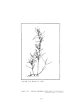 Since the staminate flower is only a couple of millimeters away from the
stigmatic surfaces of the carpels at maturity, it is possible that this species
reproduces by selfing. The hyaline membranous cup around the base of the car-
pels may help in pollen capture. Fruit development is very rapid. In the
Chesapeake Bay, seeds are found very early in the year, almost as soon as veg-
etative shoot growth begins. The fruit with its persistent horn-shaped style
gives this species the common name of horned pondweed. Technically the fruit
is classified as an achene (i.e., a small one-sided indehiscent structure with
thin pericarp derived from a single carpel). The body of the achene is up to
2 to 3 mm long while the style is another 1 to 2 mm.
Seed germination of Zannichellia is much more rapid than most other sub-
merged aquatics which often germinate several years after seed set. This species
has shown significant germination in the same year as the seed was set (Guppy
1897). In Lake Titicaca, Tutin (1940) found Zannichellia fruiting and germin-
ating abundantly at the same time of the year. The short life cycle of this
species may help account for its rapid colonizing ability.
Distribution
Figure 20 and Table 9 show the distribution of Zannichellia in the Chesa-
peake Bay for the 1970s based on summer survey data from MBHRL. In only two
years, 1972 and 1976, was Zannichellia found in abundance. Distribution was
centered in the Choptank River and Eastern Bay areas. In the years 1971, 1973,
1974 and 1975, survey teams found horned pondweed at one station or less. Pre-
liminary reports by various researchers indicate that populations may have re-
turned to higher levels in 1977. Confirmation from MBHRL is not available at
this time. This distribution pattern is among the more erratic of all the
Chesapeake Bay submerged aquatic species. To some extent, this may be an arti-
fact of summer surveying. Zannichellia populations seem to decline rapidly in
June and early July, so that late July and August surveys might not be adequate
to monitor this species. However, Zannichellia does appear to be an ephemeral
pioneer species which does show considerable yearly fluctuations in occurrence
off Horn Point in the Choptank River (Stevenson, personal communication).
Fenwick (personal communication) has studied Zannichellia abundance in Eastern
Bay and has suggested that Zannichellia can be easily missed in beds of mixed
species. After its early growing period, Zanni'chellia beds are often over run
by other morphologically similar species, (i.e. Ruppia). Dense Ruppia beds
tend to hide the shorter Zanm'chellia plants.
Historically in the Chesapeake Bay, this species seems tobea relative
"late comer" in the herbarium record. The earliest reported specimen from a
Bay area herbarium dates from 1931 in the Cove Point area on the Western Shore.
After that, there have been relatively few records until the 1960s. Most other
submerged aquatic species are documented in herbaria before the 1900s in the
Chesapeake Bay. This may indicate that Zannichellia has been established re-
latively recently or at least was in relatively low frequencies in the Chesapeake
in the past. However, paleopollen studies of Bay sediments would be necessary
to confirm or reject this hypothesis.
Zanni'chelli'a palustris is remarkably cosmopolitan. Clapham et al. (1952)
reported that it was a native of the British Isles and is locally common in
67
image:
Since the staminate flower is only a couple of millimeters away from the
stigmatic surfaces of the carpels at maturity, it is possible that this species
reproduces by selfing. The hyaline membranous cup around the base of the car-
pels may help in pollen capture. Fruit development is very rapid. In the
Chesapeake Bay, seeds are found very early in the year, almost as soon as veg-
etative shoot growth begins. The fruit with its persistent horn-shaped style
gives this species the common name of horned pondweed. Technically the fruit
is classified as an achene (i.e., a small one-sided indehiscent structure with
thin pericarp derived from a single carpel). The body of the achene is up to
2 to 3 mm long while the style is another 1 to 2 mm.
Seed germination of Zannichellia is much more rapid than most other sub-
merged aquatics which often germinate several years after seed set. This species
has shown significant germination in the same year as the seed was set (Guppy
1897). In Lake Titicaca, Tutin (1940) found Zannichellia fruiting and germin-
ating abundantly at the same time of the year. The short life cycle of this
species may help account for its rapid colonizing ability.
Distribution
Figure 20 and Table 9 show the distribution of Zannichellia in the Chesa-
peake Bay for the 1970s based on summer survey data from MBHRL. In only two
years, 1972 and 1976, was Zannichellia found in abundance. Distribution was
centered in the Choptank River and Eastern Bay areas. In the years 1971, 1973,
1974 and 1975, survey teams found horned pondweed at one station or less. Pre-
liminary reports by various researchers indicate that populations may have re-
turned to higher levels in 1977. Confirmation from MBHRL is not available at
this time. This distribution pattern is among the more erratic of all the
Chesapeake Bay submerged aquatic species. To some extent, this may be an arti-
fact of summer surveying. Zannichellia populations seem to decline rapidly in
June and early July, so that late July and August surveys might not be adequate
to monitor this species. However, Zannichellia does appear to be an ephemeral
pioneer species which does show considerable yearly fluctuations in occurrence
off Horn Point in the Choptank River (Stevenson, personal communication).
Fenwick (personal communication) has studied Zannichellia abundance in Eastern
Bay and has suggested that Zannichellia can be easily missed in beds of mixed
species. After its early growing period, Zanni'chellia beds are often over run
by other morphologically similar species, (i.e. Ruppia). Dense Ruppia beds
tend to hide the shorter Zanm'chellia plants.
Historically in the Chesapeake Bay, this species seems tobea relative
"late comer" in the herbarium record. The earliest reported specimen from a
Bay area herbarium dates from 1931 in the Cove Point area on the Western Shore.
After that, there have been relatively few records until the 1960s. Most other
submerged aquatic species are documented in herbaria before the 1900s in the
Chesapeake Bay. This may indicate that Zannichellia has been established re-
latively recently or at least was in relatively low frequencies in the Chesapeake
in the past. However, paleopollen studies of Bay sediments would be necessary
to confirm or reject this hypothesis.
Zanni'chelli'a palustris is remarkably cosmopolitan. Clapham et al. (1952)
reported that it was a native of the British Isles and is locally common in
67
image:
 1971
1973
\
1975
Figure 20. Distribution of Zannichellia palustris, Maryland Chesapeake
Bay, 1971-1976
68
image:
1971
1973
\
1975
Figure 20. Distribution of Zannichellia palustris, Maryland Chesapeake
Bay, 1971-1976
68
image:
 Table 9. Percent of sampling stations showing occurrence of
Zanm'chell ia palustris, Maryland Chesapeake Bay, 1971-1976 a
ftrea
Code
1
2
3
4
5
6
7
8
9
10
11
12
13
14
15
16
17
18
19
20
21
22
23
24
25
26
Number of stations
River System
Elk & Bohemia
Rivers
Sassafras River
Howell & Swarm
Points
Eastern Bay
Choptank River
Little Choptank
River
James Island &
Honga River
Honga River
Bloodsworth Is.
Susquehanna Flats
Fishing Bay
Nanticoke &
Wicomico Rivers
Manokin River
Patapsco River
Big & Little
Annemessex Rivers
Gunpowder & Bush
River Headwaters
Pocomoke Sound
(Maryland)
Hagothy River
Severn River
Patuxent River
Back, Middle &
Gunpowder Rivers
Curtis & Cover
Points
South, West &
Rhode Rivers
Chester River
Love & Kent
Points
Smith Island
(Maryland)
Total
1971
0
0
0
0
0
0
0
0
0
0
0
0
0
0
0
0
0
0
0
0
0
0
0
0
0
0
0
1972
0
0
0
13.95
17.24
5.26
0
0
0
0
0
0
0
0
0
0
0
0
0
0
0
0
0
0
0
0
2.76
1973
0
0
0
0
0
0
0
0
0
0
0
0
0
0
0
0
0
0
0
0
0
0
0
2,94
0
0
0.16
1974
0
0
0
0
0
0
0
0
0
0
0
0
0
0
0
0
-
0
6.67
0
0
0
0
0
0
0
0.16
1975
0
0
0
0
0
0
0
0
0
0
0
0
0
0
0
-
0
-
-
0
0
0
0
0
0
0
0
1976
0
0
0
20.00
14.29
0
2.94
3.45
0
0
0
0
0
0
0
0
0
0
7.69
0
0
0
0
5.71
0
0
3.50
71
15
10
12
47
60
19
34
30
40
27
25
3C
15
21
20
9
22
12
15
50
22
20
8
36
8
17
624
72 73
16 16
10 10
6 12
43 47
58 57
19 19
34 34
30 30
44 46
37 37
25 25
30 30
15 15
20 21
20 20
8 7
20 21
12 12
15 15
47 50
22 22
19 19
10 10
36 34
8 8
11 12
74
16
10
12
47
58
19
34
30
43
37
25
30
15
21
19
9
-
12
15
50
22
19
8
34
8
17
615629610
75
16
10
12
46
57
19
34
29
43
36
24
30
14
0
18
-
20
-
-
47
22
6
8
36
8
17
553
76
16
10
12
45
56
19
34
29
45
35
25
30
15
21
20
9
22
12
13
49
22
21
8
35
8
17
628
U.S. Fish and Wildlife Service Migratory Bird and Habitat Research Laboratory, 1976.
69
image:
Table 9. Percent of sampling stations showing occurrence of
Zanm'chell ia palustris, Maryland Chesapeake Bay, 1971-1976 a
ftrea
Code
1
2
3
4
5
6
7
8
9
10
11
12
13
14
15
16
17
18
19
20
21
22
23
24
25
26
Number of stations
River System
Elk & Bohemia
Rivers
Sassafras River
Howell & Swarm
Points
Eastern Bay
Choptank River
Little Choptank
River
James Island &
Honga River
Honga River
Bloodsworth Is.
Susquehanna Flats
Fishing Bay
Nanticoke &
Wicomico Rivers
Manokin River
Patapsco River
Big & Little
Annemessex Rivers
Gunpowder & Bush
River Headwaters
Pocomoke Sound
(Maryland)
Hagothy River
Severn River
Patuxent River
Back, Middle &
Gunpowder Rivers
Curtis & Cover
Points
South, West &
Rhode Rivers
Chester River
Love & Kent
Points
Smith Island
(Maryland)
Total
1971
0
0
0
0
0
0
0
0
0
0
0
0
0
0
0
0
0
0
0
0
0
0
0
0
0
0
0
1972
0
0
0
13.95
17.24
5.26
0
0
0
0
0
0
0
0
0
0
0
0
0
0
0
0
0
0
0
0
2.76
1973
0
0
0
0
0
0
0
0
0
0
0
0
0
0
0
0
0
0
0
0
0
0
0
2,94
0
0
0.16
1974
0
0
0
0
0
0
0
0
0
0
0
0
0
0
0
0
-
0
6.67
0
0
0
0
0
0
0
0.16
1975
0
0
0
0
0
0
0
0
0
0
0
0
0
0
0
-
0
-
-
0
0
0
0
0
0
0
0
1976
0
0
0
20.00
14.29
0
2.94
3.45
0
0
0
0
0
0
0
0
0
0
7.69
0
0
0
0
5.71
0
0
3.50
71
15
10
12
47
60
19
34
30
40
27
25
3C
15
21
20
9
22
12
15
50
22
20
8
36
8
17
624
72 73
16 16
10 10
6 12
43 47
58 57
19 19
34 34
30 30
44 46
37 37
25 25
30 30
15 15
20 21
20 20
8 7
20 21
12 12
15 15
47 50
22 22
19 19
10 10
36 34
8 8
11 12
74
16
10
12
47
58
19
34
30
43
37
25
30
15
21
19
9
-
12
15
50
22
19
8
34
8
17
615629610
75
16
10
12
46
57
19
34
29
43
36
24
30
14
0
18
-
20
-
-
47
22
6
8
36
8
17
553
76
16
10
12
45
56
19
34
29
45
35
25
30
15
21
20
9
22
12
13
49
22
21
8
35
8
17
628
U.S. Fish and Wildlife Service Migratory Bird and Habitat Research Laboratory, 1976.
69
image:
 rivers, streams, ditches and brackish pools. It is also widespread throughout
Europe where Reese (1963) documented several chromosome races. The species is
also well distributed in the Old World.
In North America, Porsild (1932) reported Zannichellia palustris within
the Artie Circle on the north coast of the Seward Penninsula in the Buckland
River delta region. Although this species has been documented in every state in
the continental United States (Fassett I960), it is not a commonly occurring
submerged aquatic. Deane (1910) reported that Zannichellia could be found only
occasionally in brackish marshes along the New England coast, but it rarely
occurred inland. South of the Chesapeake Bay, this species can be found in
abundance in the Currituck and Pamlico Sound areas in North Carolina. However,
in South Carolina and the southern Coastal Plain counties of North Carolina,
Zannichellia is relatively rare.
In South America, this species has been found in Lake Titicaca located at
3,815 m in the Andes Mountains (Hutchinson 1975). The widespread occurrence
of this species even at such remote locations suggests excellent dispersal
mechanisms as well as a wide range of adaptability to varying climates and
altitudes.
Environmental Factors Affecting Distribution
Temperature. Comparatively little information is available from the litera-
ture on how physical environment and water quality parameters affect this species.
There are indications in the Chesapeake Bay that this species may be sensitive
to high water temperatures. As summer approaches and water temperatures in-
crease above 30 C, Zannichellia populations often begin to decline rapidly.
However, it is unclear whether this is a strict temperature effect or whether
other variables are involved. Fenwick (personal communication) found healthy
Zannichellia growing in Eastern Neck (Eastern Bay area) tidal pools where the
temperature often exceeded 38 C. Porsild (1932) indicated that this species
was found in hot springs in Kamchatka (USSR) where water temperatures varied
from 25 to 30 C. At the lower end of the temperature range is Lake Titicaca
where Tutin (1940) reported Zannichellia populations existed in a temperature
range from 10.5 to 14.8 C.
Salinity. Horned pondweed is able to persist in fresh water, but there
seems to be a definite preference of this species for brackish areas or cal-
careous pools (Radford et al. 1964) and hard water situations (Fassett 1960).
In the Chesapeake Bay this species has been found as far south as the mouth
of the Honga River. Salinities seldom go beyond 20 ppt in this area so this
may be the maximum limit of salinity tolerance for Zannichellia in the Chesapeake
Bay.
Sediments. Zanm'chellia has a tendency to grow in clay to sandy sediments
in shallower water than other submerged aquatics in the Chesapeake Bay. This
is also the case in Lake Titicaca where Tutin found Zannichellia in the shallow-
est situations whereas Potamogeton, Myriophyllum and El odea dominated the deep-
er waters. This suggests that Zannichellia may need higher light intensities
than other submerged aquatics for optimal growth. Correll et al. (1977) sub-
jected Zannichellia to 80 to 140 yE/m2/sec at the water surface (approximately
70
image:
rivers, streams, ditches and brackish pools. It is also widespread throughout
Europe where Reese (1963) documented several chromosome races. The species is
also well distributed in the Old World.
In North America, Porsild (1932) reported Zannichellia palustris within
the Artie Circle on the north coast of the Seward Penninsula in the Buckland
River delta region. Although this species has been documented in every state in
the continental United States (Fassett I960), it is not a commonly occurring
submerged aquatic. Deane (1910) reported that Zannichellia could be found only
occasionally in brackish marshes along the New England coast, but it rarely
occurred inland. South of the Chesapeake Bay, this species can be found in
abundance in the Currituck and Pamlico Sound areas in North Carolina. However,
in South Carolina and the southern Coastal Plain counties of North Carolina,
Zannichellia is relatively rare.
In South America, this species has been found in Lake Titicaca located at
3,815 m in the Andes Mountains (Hutchinson 1975). The widespread occurrence
of this species even at such remote locations suggests excellent dispersal
mechanisms as well as a wide range of adaptability to varying climates and
altitudes.
Environmental Factors Affecting Distribution
Temperature. Comparatively little information is available from the litera-
ture on how physical environment and water quality parameters affect this species.
There are indications in the Chesapeake Bay that this species may be sensitive
to high water temperatures. As summer approaches and water temperatures in-
crease above 30 C, Zannichellia populations often begin to decline rapidly.
However, it is unclear whether this is a strict temperature effect or whether
other variables are involved. Fenwick (personal communication) found healthy
Zannichellia growing in Eastern Neck (Eastern Bay area) tidal pools where the
temperature often exceeded 38 C. Porsild (1932) indicated that this species
was found in hot springs in Kamchatka (USSR) where water temperatures varied
from 25 to 30 C. At the lower end of the temperature range is Lake Titicaca
where Tutin (1940) reported Zannichellia populations existed in a temperature
range from 10.5 to 14.8 C.
Salinity. Horned pondweed is able to persist in fresh water, but there
seems to be a definite preference of this species for brackish areas or cal-
careous pools (Radford et al. 1964) and hard water situations (Fassett 1960).
In the Chesapeake Bay this species has been found as far south as the mouth
of the Honga River. Salinities seldom go beyond 20 ppt in this area so this
may be the maximum limit of salinity tolerance for Zannichellia in the Chesapeake
Bay.
Sediments. Zanm'chellia has a tendency to grow in clay to sandy sediments
in shallower water than other submerged aquatics in the Chesapeake Bay. This
is also the case in Lake Titicaca where Tutin found Zannichellia in the shallow-
est situations whereas Potamogeton, Myriophyllum and El odea dominated the deep-
er waters. This suggests that Zannichellia may need higher light intensities
than other submerged aquatics for optimal growth. Correll et al. (1977) sub-
jected Zannichellia to 80 to 140 yE/m2/sec at the water surface (approximately
70
image:
 4 to 7 percent of the maximum noon summer sunlight)and obtained good growth.
Little else is available concerning the light requirements of this species.
Current, Wind and Wave Action. In the Chesapeake, Zannichellia grows in
shallow areas where up to one knot currents develop. Sculthorpe (1967) mention-
ed that the adventitious roots of this species are spiral, tendril-like and aid
in anchorage. The rhizomes of this species are very slender and would other-
wise be easily dislodged in strong currents without the adventitious root
system. However, this adaptation is apparently not effective where wave action
is significant, since this species is never found on high energy shorelines.
Zannichellia was one of the -few submerged aquatics that did well in the
Chesapeake Bay after Hurricane AGNES when much sediment was deposited on the
Bay bottom. The adaptive strategy of this species in regard to sedimentation
seems to be toward rapid recolonization, rather than growing up through sedi-
ments which are being rapidly deposited. No information is available on how
well this species does in regard to trapping sediments and reducing turbidity.
However, its filiform leaves and slender rhizomes are probably not as effective
in this regard as Myriophyllum and other species which grow in thick masses.
In terms of water quality responses, Zannichellia may be associated with
increased nutrient loading. In reviewing some of the work on central European
Lakes, Hutchinson (1975) indicated that Zannichellia was an important species
in eutrophic waters. In mesotrophic locations, Najas displaced Zannichellia
as a codominant with narrow leaved Potamogeton species. Zannichellia has been
found in recent surveys of Lake Mendota. This lake has been undergoing rapid
eutrophication since the early 1900s. Hutchinson (1975) cited early surveys of
Lake Mendota in 1912, 1922 and 1940 as having found no Zannichellia. Recent
work by Lind and Cottam (1969) showed that Zannichellia appeared in the lake in
the shallowest emersed zone while Myriophyllum exalbescens formed monospecific
stands in deeper waters. Since Zannichellia, as mentioned previously, has only
been widely established in the Chesapeake Bay since the 1960s, it is possible
that its spread may be an indicator of increased eutrophication of the Bay.
However, Zannichellia is not found in all eutrophic waters of the Chesapeake Bay.
Productivity
The only productivity data available for Zannichellia comes from in situ
measurements in the Rhode River, a subestuary of the Chesapeake Bay. Correll
et al. (1977) measured oxygen metabolism of plants placed in glass bottles at
depths of 20 and 40 cm below the surface. At 20 cm net oxygen production was
calculated to be 462 mg 02/9 dry weight tissue while at 40 cm it was 298 mg, 02/g
dry weight tissue. Net photosynthesis was 26.0 mg 02/hr/g dry weight at 20 cm
and 22.0 mg 02hr/g dry weight at 40 cm. Respiration measured in dark bottles
was 6.3 mg 02/hr/g dry weight at 20 cm and 7.1 mg 02/hr/g dry weight at 40 cm.
Unfortunately, there is presently little comparative data for other submerged
aquatics using similar techniques.
Consumer Utilization
Fassett (1960) reported that fruits and sometimes foliage of Zannichellia
are good for waterfowl in brackish pools. Furthermore, it was rated by
71
image:
4 to 7 percent of the maximum noon summer sunlight)and obtained good growth.
Little else is available concerning the light requirements of this species.
Current, Wind and Wave Action. In the Chesapeake, Zannichellia grows in
shallow areas where up to one knot currents develop. Sculthorpe (1967) mention-
ed that the adventitious roots of this species are spiral, tendril-like and aid
in anchorage. The rhizomes of this species are very slender and would other-
wise be easily dislodged in strong currents without the adventitious root
system. However, this adaptation is apparently not effective where wave action
is significant, since this species is never found on high energy shorelines.
Zannichellia was one of the -few submerged aquatics that did well in the
Chesapeake Bay after Hurricane AGNES when much sediment was deposited on the
Bay bottom. The adaptive strategy of this species in regard to sedimentation
seems to be toward rapid recolonization, rather than growing up through sedi-
ments which are being rapidly deposited. No information is available on how
well this species does in regard to trapping sediments and reducing turbidity.
However, its filiform leaves and slender rhizomes are probably not as effective
in this regard as Myriophyllum and other species which grow in thick masses.
In terms of water quality responses, Zannichellia may be associated with
increased nutrient loading. In reviewing some of the work on central European
Lakes, Hutchinson (1975) indicated that Zannichellia was an important species
in eutrophic waters. In mesotrophic locations, Najas displaced Zannichellia
as a codominant with narrow leaved Potamogeton species. Zannichellia has been
found in recent surveys of Lake Mendota. This lake has been undergoing rapid
eutrophication since the early 1900s. Hutchinson (1975) cited early surveys of
Lake Mendota in 1912, 1922 and 1940 as having found no Zannichellia. Recent
work by Lind and Cottam (1969) showed that Zannichellia appeared in the lake in
the shallowest emersed zone while Myriophyllum exalbescens formed monospecific
stands in deeper waters. Since Zannichellia, as mentioned previously, has only
been widely established in the Chesapeake Bay since the 1960s, it is possible
that its spread may be an indicator of increased eutrophication of the Bay.
However, Zannichellia is not found in all eutrophic waters of the Chesapeake Bay.
Productivity
The only productivity data available for Zannichellia comes from in situ
measurements in the Rhode River, a subestuary of the Chesapeake Bay. Correll
et al. (1977) measured oxygen metabolism of plants placed in glass bottles at
depths of 20 and 40 cm below the surface. At 20 cm net oxygen production was
calculated to be 462 mg 02/9 dry weight tissue while at 40 cm it was 298 mg, 02/g
dry weight tissue. Net photosynthesis was 26.0 mg 02/hr/g dry weight at 20 cm
and 22.0 mg 02hr/g dry weight at 40 cm. Respiration measured in dark bottles
was 6.3 mg 02/hr/g dry weight at 20 cm and 7.1 mg 02/hr/g dry weight at 40 cm.
Unfortunately, there is presently little comparative data for other submerged
aquatics using similar techniques.
Consumer Utilization
Fassett (1960) reported that fruits and sometimes foliage of Zannichellia
are good for waterfowl in brackish pools. Furthermore, it was rated by
71
image:
 Needham (1938) as a fair food producer for trout. However, Ruppia, Vallisneria
and Potamogeton spp. are usually considered more important in nourishing fish
and wildlife species.
Economic Uses and Problems
This species has not reached the epidemic proportion in terms of population
size as did Myriophyllum. Therefore, there are no particular problems in the
Chesapeake Bay associated with its occurrence. Since it is a pioneer species,
it may be helpful in revegetating areas where it is desirable to have submerged
aquatics. Little use has been made of Zannichellia for this purpose up to the
present time.
VALLISNERIA AMERICANA
Biology
General Vegetative Morphology. Often referred to as wild celery, tape grass
or eel-grass, Vallisneria americana belongs to the Hydrocharitaceae family along
with El odea. V_. americana, _V. asiatica and V^ aethiopica are thought by some
botanists to be geographic races of V_. spiral is (Sculthorpe 1967). Fassett
(1960) used the name V_. americana and listed V_. spiral is as a synonym referenced
with Gray's Manual and Britton and Brown. The name _V. americana will be used
for the purpose of this document.
Vallisneria americana is a monocotolydon, with ribbon or strap-shaped trans-
lucent leaves, 3 to 10 mm wide and arranged in basal clusters at the ends of
creeping stems (Schuette and Alder 1927; Sculthorpe 1967; Radford et al. 1964;
Needham and Lloyd 1930) (see Figure 21). Leaves may attain up to 1.8 m in length
with the height of the plant more or less limtied by water depth (Schuette and
Alder 1927).
Reproduction. Vegetative propogation occurs primarily through the vigorous
growth of stolons or runners and through tubers (Sculthorpe 1967; Lamoureux 1957).
Sexual reproduction is more complex. Pistillate flowers are borne on peduncles
that elongate at anthesis until they reach the water surface. Staminate flowers,
by comparison, are free-floating after having broken away from the plant base at
anthesis. Once fertilization has occurred at the water/air interface, the
pistillate peduncles coil downwards and submerge the many seeded, berry-like
fruit (Sculthorpe 1967; Muenscher 1936).
Distribution
Wild celery is considered to be a fresh water macrophyte occurring in the
tidal streams of the Atlantic Coastal Plain (Martin and Uhler 1939).
The summer sampling conducted by MBHRL has documented V_. americana in the
Chesapeake Bay from 1971 through 1976. Though the data is sparse (see Table 10
and Figure 22) species occurrence shows a decline over the six year period. In
1971, wild celery was well represented in the Susquehanna Flats. By 1973, those
same stations were bare of wild celery and subsequent sampling has not shown any
72
image:
Needham (1938) as a fair food producer for trout. However, Ruppia, Vallisneria
and Potamogeton spp. are usually considered more important in nourishing fish
and wildlife species.
Economic Uses and Problems
This species has not reached the epidemic proportion in terms of population
size as did Myriophyllum. Therefore, there are no particular problems in the
Chesapeake Bay associated with its occurrence. Since it is a pioneer species,
it may be helpful in revegetating areas where it is desirable to have submerged
aquatics. Little use has been made of Zannichellia for this purpose up to the
present time.
VALLISNERIA AMERICANA
Biology
General Vegetative Morphology. Often referred to as wild celery, tape grass
or eel-grass, Vallisneria americana belongs to the Hydrocharitaceae family along
with El odea. V_. americana, _V. asiatica and V^ aethiopica are thought by some
botanists to be geographic races of V_. spiral is (Sculthorpe 1967). Fassett
(1960) used the name V_. americana and listed V_. spiral is as a synonym referenced
with Gray's Manual and Britton and Brown. The name _V. americana will be used
for the purpose of this document.
Vallisneria americana is a monocotolydon, with ribbon or strap-shaped trans-
lucent leaves, 3 to 10 mm wide and arranged in basal clusters at the ends of
creeping stems (Schuette and Alder 1927; Sculthorpe 1967; Radford et al. 1964;
Needham and Lloyd 1930) (see Figure 21). Leaves may attain up to 1.8 m in length
with the height of the plant more or less limtied by water depth (Schuette and
Alder 1927).
Reproduction. Vegetative propogation occurs primarily through the vigorous
growth of stolons or runners and through tubers (Sculthorpe 1967; Lamoureux 1957).
Sexual reproduction is more complex. Pistillate flowers are borne on peduncles
that elongate at anthesis until they reach the water surface. Staminate flowers,
by comparison, are free-floating after having broken away from the plant base at
anthesis. Once fertilization has occurred at the water/air interface, the
pistillate peduncles coil downwards and submerge the many seeded, berry-like
fruit (Sculthorpe 1967; Muenscher 1936).
Distribution
Wild celery is considered to be a fresh water macrophyte occurring in the
tidal streams of the Atlantic Coastal Plain (Martin and Uhler 1939).
The summer sampling conducted by MBHRL has documented V_. americana in the
Chesapeake Bay from 1971 through 1976. Though the data is sparse (see Table 10
and Figure 22) species occurrence shows a decline over the six year period. In
1971, wild celery was well represented in the Susquehanna Flats. By 1973, those
same stations were bare of wild celery and subsequent sampling has not shown any
72
image:
 (copied from Hotchkiss 1967)
Figure 21. Wildcelery (Vallisneria americana)
73
image:
(copied from Hotchkiss 1967)
Figure 21. Wildcelery (Vallisneria americana)
73
image:
 Table 10. Percent of sampling stations showing occurrence of
Vailisneria americana, Maryland Chesapeake Bay, 1971-19763
Area
Code
1
2
3
4
5
6
7
8
9
10
11
12
13
14
15
16
17
18
19
20
21
22
23
24
25
26
Number of
River system
Elk & Bohemia
Rivers
Sassafras River
Howell & Swann
Points
Eastern Bay
Choptank River
Little Choptank
River
James Island &
Honga River
Honga River
Bloodsworth Is.
Susquehanna
Flats
Fishing Bay
Nanticoke &
Wicomico Rivers
Manokin River
Patapsco River
Big & Little
Annemessex Rivers
Gunpowder & Bush
River Headwaters
Pocomoke Sound
(Maryland)
Magothy River
Severn River
Patuxent River
Back, Middle &
Gunpowder Rivers
Curtis & Cove
Points
South, West &
Rhode Rivers
Chester River
Love & Kent
Points
Smith Island
(Maryland)
Total
1971
6.67
20.00
8.33
0
0
0
0
0
0
37.04
0
0
0
0
0
0
0
16.67
0
0
0
0
0
2.78
0
0
2.72
1972
0
0
0
0
0
0
0
0
0
2.70
0
0
0
0
0
0
0
0
0
0
0
0
0
0
0
0
0.16
1973
0
0
0
0
0
0
0
0
0
0
0
0
0
4.76
0
0
0
8.33
0
0
0
0
0
2.94
0
0
0.48
1974
0
0
0
0
0
0
0
0
0
0
0
0
0
9.52
0
0
0
0
0
0
4.55
0
0
5.88
0
0
0.82
1975
0
0
0
0
0
0
0
0
0
0
0
0
0
-
0
-
0
-
-
0
9.09
0
0
8.33
0
0
0.90
1976
0
0
0
0
0
0
0
0
0
0
0
0
0
9.52
0
0
0
8.33
0
0
0
0
0
2.86
0
0
0.64
71
15
10
12
47
60
19
34
30
40
27
25
30
15
21
20
9
22
12
15
50
22
20
8
36
8
17
624
72
16
10
6
43
58
19
34
30
44
37
25
30
15
20
20
8
20
12
15
47
22
19
10
36
8
11
615
/3
16
10
12
47
57
19
34
30
46
37
25
30
15
21
20
7
21
12
15
50
22
19
10
34
8
12
629
stations
74
16
10
12
47
58
19
34
30
43
37
25
30
15
21
19
9
0
12
15
50
22
19
8
34
8
17
610
/b
16
10
12
46
57
19
34
29
43
36
24
30
14
-
18
-
20
-
-
47
22
6
8
36
8
17
553
76
16
10
12
45
56
19
34
29
45
35
25
30
15
21
20
9
22
12
13
49
22
21
8
35
8
17
628
a
U.S. Fish and Wildlife Service Migratory Bird and Habitat Research Laboratory, 1976
74
image:
Table 10. Percent of sampling stations showing occurrence of
Vailisneria americana, Maryland Chesapeake Bay, 1971-19763
Area
Code
1
2
3
4
5
6
7
8
9
10
11
12
13
14
15
16
17
18
19
20
21
22
23
24
25
26
Number of
River system
Elk & Bohemia
Rivers
Sassafras River
Howell & Swann
Points
Eastern Bay
Choptank River
Little Choptank
River
James Island &
Honga River
Honga River
Bloodsworth Is.
Susquehanna
Flats
Fishing Bay
Nanticoke &
Wicomico Rivers
Manokin River
Patapsco River
Big & Little
Annemessex Rivers
Gunpowder & Bush
River Headwaters
Pocomoke Sound
(Maryland)
Magothy River
Severn River
Patuxent River
Back, Middle &
Gunpowder Rivers
Curtis & Cove
Points
South, West &
Rhode Rivers
Chester River
Love & Kent
Points
Smith Island
(Maryland)
Total
1971
6.67
20.00
8.33
0
0
0
0
0
0
37.04
0
0
0
0
0
0
0
16.67
0
0
0
0
0
2.78
0
0
2.72
1972
0
0
0
0
0
0
0
0
0
2.70
0
0
0
0
0
0
0
0
0
0
0
0
0
0
0
0
0.16
1973
0
0
0
0
0
0
0
0
0
0
0
0
0
4.76
0
0
0
8.33
0
0
0
0
0
2.94
0
0
0.48
1974
0
0
0
0
0
0
0
0
0
0
0
0
0
9.52
0
0
0
0
0
0
4.55
0
0
5.88
0
0
0.82
1975
0
0
0
0
0
0
0
0
0
0
0
0
0
-
0
-
0
-
-
0
9.09
0
0
8.33
0
0
0.90
1976
0
0
0
0
0
0
0
0
0
0
0
0
0
9.52
0
0
0
8.33
0
0
0
0
0
2.86
0
0
0.64
71
15
10
12
47
60
19
34
30
40
27
25
30
15
21
20
9
22
12
15
50
22
20
8
36
8
17
624
72
16
10
6
43
58
19
34
30
44
37
25
30
15
20
20
8
20
12
15
47
22
19
10
36
8
11
615
/3
16
10
12
47
57
19
34
30
46
37
25
30
15
21
20
7
21
12
15
50
22
19
10
34
8
12
629
stations
74
16
10
12
47
58
19
34
30
43
37
25
30
15
21
19
9
0
12
15
50
22
19
8
34
8
17
610
/b
16
10
12
46
57
19
34
29
43
36
24
30
14
-
18
-
20
-
-
47
22
6
8
36
8
17
553
76
16
10
12
45
56
19
34
29
45
35
25
30
15
21
20
9
22
12
13
49
22
21
8
35
8
17
628
a
U.S. Fish and Wildlife Service Migratory Bird and Habitat Research Laboratory, 1976
74
image:
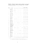 Figure 22. Distribution of Vallisneria americana, Maryland Chesapeake
Bay, 1971-1976 ~
75
image:
Figure 22. Distribution of Vallisneria americana, Maryland Chesapeake
Bay, 1971-1976 ~
75
image:
 any return of the species. Data for 1977 is not available at the present time
for individual species.
A further study conducted by Bayley et al. (in press) in the Susquehanna
Flats over the period 1958 to 1975 supports the species decline noted in the
previous study. A drastic decline in the Flats was noted after 1971. Prior to
1971, in the early and mid 1960s, Vallisneria seemed to have been impacted by the
explosive growth of Myriophyllum spicatum.
Environmental Factors Effecting Distribution
Temperature. Laboratory tests (Wilkinson 1963) showed that Vallisneria
grew best within a temperature range of 33 to 36 C. Arrested growth occurred
below 19 C; and above 50 C plants became limp and disintegrated. Wild celery
has not been found to overwinter in green form (Lind and Cottam 1969).
Salinity. Bourn (1934) found that Vallisneria could not be successfully
maintained under laboratory conditions with a salinity concentration greater
than 4.2 ppt. Growth was slightly stimulated by increasing concentrations of
saltwater up to 8 percent; however, this stimulation resulted in only a very
slight increase in dry weight when compared to fresh-water grown control plants.
Etiolation was noted in plants grown in upwards of 6.6 ppt.
Studies in Currituck Sound (Bureau of Sport Fisheries and Wildlife 1965)
concluded that wild celery plants were capable of tolerating higher salinities
when grown in a silt substrate rather than sand. This possibly was due to the
high cation exchange in silt soils that protected the root structure. Sand
substrates were not found to have the same buffering capacity.
Substrate. Schuette and Alder (1927) found that V. americana grew equally
well in sandy soil and mud. However, in Lake Mendota, Wisconsin, wild celery
was observed growing only on sandy substrate (Lind and Cottam 1969). In experi-
ments utilizing different types of soils, Hutchinson (1975) found that
X- americana thrived best in a soil composed of:
6.50 percent organics
8.78 percent gravel
21.46 percent sand
47.90 percent silt
14.26 percent clay
Light, Depth and Turbidity. Vallisneria americana has been found to be
tolerant of muddy, roiled water (Steenis 1970). Lake studies (Meyer et al. 1943)
demonstrated that V^. americana was able to maintain 25 percent of its surface
photosynthetic rate at a depth of 10 m where the prevailing light intensity was
0.5 percent of surface light on the clearest days. In northern Currituck Sound,
North Carolina, during the summer and fall, 1977, Vallisneria americana was
invariably found in shallow water (0.5 to 1.0 m) compared to MyriophyHum spicatum
76
image:
any return of the species. Data for 1977 is not available at the present time
for individual species.
A further study conducted by Bayley et al. (in press) in the Susquehanna
Flats over the period 1958 to 1975 supports the species decline noted in the
previous study. A drastic decline in the Flats was noted after 1971. Prior to
1971, in the early and mid 1960s, Vallisneria seemed to have been impacted by the
explosive growth of Myriophyllum spicatum.
Environmental Factors Effecting Distribution
Temperature. Laboratory tests (Wilkinson 1963) showed that Vallisneria
grew best within a temperature range of 33 to 36 C. Arrested growth occurred
below 19 C; and above 50 C plants became limp and disintegrated. Wild celery
has not been found to overwinter in green form (Lind and Cottam 1969).
Salinity. Bourn (1934) found that Vallisneria could not be successfully
maintained under laboratory conditions with a salinity concentration greater
than 4.2 ppt. Growth was slightly stimulated by increasing concentrations of
saltwater up to 8 percent; however, this stimulation resulted in only a very
slight increase in dry weight when compared to fresh-water grown control plants.
Etiolation was noted in plants grown in upwards of 6.6 ppt.
Studies in Currituck Sound (Bureau of Sport Fisheries and Wildlife 1965)
concluded that wild celery plants were capable of tolerating higher salinities
when grown in a silt substrate rather than sand. This possibly was due to the
high cation exchange in silt soils that protected the root structure. Sand
substrates were not found to have the same buffering capacity.
Substrate. Schuette and Alder (1927) found that V. americana grew equally
well in sandy soil and mud. However, in Lake Mendota, Wisconsin, wild celery
was observed growing only on sandy substrate (Lind and Cottam 1969). In experi-
ments utilizing different types of soils, Hutchinson (1975) found that
X- americana thrived best in a soil composed of:
6.50 percent organics
8.78 percent gravel
21.46 percent sand
47.90 percent silt
14.26 percent clay
Light, Depth and Turbidity. Vallisneria americana has been found to be
tolerant of muddy, roiled water (Steenis 1970). Lake studies (Meyer et al. 1943)
demonstrated that V^. americana was able to maintain 25 percent of its surface
photosynthetic rate at a depth of 10 m where the prevailing light intensity was
0.5 percent of surface light on the clearest days. In northern Currituck Sound,
North Carolina, during the summer and fall, 1977, Vallisneria americana was
invariably found in shallow water (0.5 to 1.0 m) compared to MyriophyHum spicatum
76
image:
 which was dominant in the deeper areas (1.0 to 2.0 m). This
suggests that VaTlisneria nay require higher light intensities for optimal
growth than other SAV species, specifically milfoil (Confer, personal observa-
ti on).
Current Velocity, Wind and Have Action. Extensive damage to Vallisneria
can occur from severe natural wave turbulence and from the action of motorboat
propellers (Lamoureux 1957).
Nutrient Responses. In assessing the role of Vallisneria in nutrient
cycles, wild celery was found to remove more silica, phosphorus, iron, aluminum,
manganese, lime, potassium and sodium than Potamogeton spp. but less sulphur,
nitrogen and magnesium (Schuette and Alder 1927).
Susceptibility. Table 11 lists various chemical agents that have been
used experimentally to eradicate Val 1i sneri a americana.
Table 11. Effects of selected herbicides on Vallisneria americana3
Herbicide
Si 1 vex
Diquat dibromide
Diquat dichloride
Paraquat dichloride
2,4-D IOE
2,4-D D, E
Acrolein
Endothall, DSS
Application
rate
Central
0.5 to 2 ppm
5 to 30 ppm
2 ppm
0.25 ppm
0.25 to 0.5 ppm
0.25 to 0.5 ppm
16.5 to 27.5 kg/ha granules
44 kg/ha granules
2.55 ppm
2 to 3 ppm
None
70 to 100%
Satisfactory
30 to 90%
30 to 100%
67 to 93%
Unsatisfactory
None
Killed
Seasonal
Lawrence and Hollingsworth 1969
Consumer Utilization
All parts of the plant structure of V_. ameri cana are consumed by fish,
ducks, coots, geese, grebes, swans, waders, shore and game birds. Wild celery
77
image:
which was dominant in the deeper areas (1.0 to 2.0 m). This
suggests that VaTlisneria nay require higher light intensities for optimal
growth than other SAV species, specifically milfoil (Confer, personal observa-
ti on).
Current Velocity, Wind and Have Action. Extensive damage to Vallisneria
can occur from severe natural wave turbulence and from the action of motorboat
propellers (Lamoureux 1957).
Nutrient Responses. In assessing the role of Vallisneria in nutrient
cycles, wild celery was found to remove more silica, phosphorus, iron, aluminum,
manganese, lime, potassium and sodium than Potamogeton spp. but less sulphur,
nitrogen and magnesium (Schuette and Alder 1927).
Susceptibility. Table 11 lists various chemical agents that have been
used experimentally to eradicate Val 1i sneri a americana.
Table 11. Effects of selected herbicides on Vallisneria americana3
Herbicide
Si 1 vex
Diquat dibromide
Diquat dichloride
Paraquat dichloride
2,4-D IOE
2,4-D D, E
Acrolein
Endothall, DSS
Application
rate
Central
0.5 to 2 ppm
5 to 30 ppm
2 ppm
0.25 ppm
0.25 to 0.5 ppm
0.25 to 0.5 ppm
16.5 to 27.5 kg/ha granules
44 kg/ha granules
2.55 ppm
2 to 3 ppm
None
70 to 100%
Satisfactory
30 to 90%
30 to 100%
67 to 93%
Unsatisfactory
None
Killed
Seasonal
Lawrence and Hollingsworth 1969
Consumer Utilization
All parts of the plant structure of V_. ameri cana are consumed by fish,
ducks, coots, geese, grebes, swans, waders, shore and game birds. Wild celery
77
image:
 further serves as a shade, shelter and spawning medium for fish, (Sculthorpe
1967), Abundant aquatic insect life has also been observed on and about wild
celery plants (Fassett 1960; Lamoureux 1957).
An infusion prepared from Vallisneria leaves has historically served as
an invigorating tonic (Sculthorpe 1967).
Economic Uses a'nd Problems
Impoundments. Use has been m^ide of Vallisneria americana for waterfowl
food in waterfowl management in the southeast (Ball 1965).However, due to
natural plant succession and almost certain invasion by pest plants in fresh
or low saline areas, beneficial results were found to be temporary unless
strenuous management practices were employed.
ELODEA CANADENSIS
Biology
General Vegetative Morphology. El odea canadensis is a member of the
Hydrocharitaceae family and is commonly referred to as waterweed (U.S. Army
Corps of Engineers 1974). Endemic to North America and naturalized to many
"industrialized nations of Europe and the southern hemisphere, this species has
long been recognized as an aquatic weed with great ability to colonize new
environments and nutrient enriched waters (Adams et al. 1971). It is also known
as both Anacharis and Elodea planchonii. The later name results from the tax-
onomic classification of a rare hermaphroditic condition of Elodea canadensis.
The term Anacharis is an acceptable name which includes both dioecious and
hermaphrodite species. Elodea canadensis, however, applies only to the dioecious
species which is characteristic of those normal specimens found in North America
(Weatherby 1932).
Mason (1969) characterized El odea as having slender stems and leaves in
threes with the lower ones opposite, ovate-oblong, acute, whorled, crowded and
overlapping near the tips (see Figure 23). The staminate flowers are solitary,
long-remaining and attached by a long peduncle, while the pistillate flowers are
solitary and sessile. The fruit is linear or lanceolate-linear. The plants are
submersed with branching stems forming large masses near the bottom (Fassett
I960).
Fragments of Elodea have been known to survive lengthy periods of exposure
(Hutchinson 1975). Introduction to formerly uncolonized areas has commonly lead
to massive proliferation. Evidence suggests that ordinarily large populations
that develop after a region has been invaded are temporary and may be expected
to decline naturally without apparent reason. Portions that break off from the
plant do not usually die, but regenerate to form new plants. Efficient produc-
tion of a large number of vegetative propagules has allowed almost complete
independence from sexual reproduction (Mitchell 1974). These segments, in-
cluding stem apices and small branches, are usually specialized asexual pro-
pagules that can overwinter (Yeo 1965bj.
78
image:
further serves as a shade, shelter and spawning medium for fish, (Sculthorpe
1967), Abundant aquatic insect life has also been observed on and about wild
celery plants (Fassett 1960; Lamoureux 1957).
An infusion prepared from Vallisneria leaves has historically served as
an invigorating tonic (Sculthorpe 1967).
Economic Uses a'nd Problems
Impoundments. Use has been m^ide of Vallisneria americana for waterfowl
food in waterfowl management in the southeast (Ball 1965).However, due to
natural plant succession and almost certain invasion by pest plants in fresh
or low saline areas, beneficial results were found to be temporary unless
strenuous management practices were employed.
ELODEA CANADENSIS
Biology
General Vegetative Morphology. El odea canadensis is a member of the
Hydrocharitaceae family and is commonly referred to as waterweed (U.S. Army
Corps of Engineers 1974). Endemic to North America and naturalized to many
"industrialized nations of Europe and the southern hemisphere, this species has
long been recognized as an aquatic weed with great ability to colonize new
environments and nutrient enriched waters (Adams et al. 1971). It is also known
as both Anacharis and Elodea planchonii. The later name results from the tax-
onomic classification of a rare hermaphroditic condition of Elodea canadensis.
The term Anacharis is an acceptable name which includes both dioecious and
hermaphrodite species. Elodea canadensis, however, applies only to the dioecious
species which is characteristic of those normal specimens found in North America
(Weatherby 1932).
Mason (1969) characterized El odea as having slender stems and leaves in
threes with the lower ones opposite, ovate-oblong, acute, whorled, crowded and
overlapping near the tips (see Figure 23). The staminate flowers are solitary,
long-remaining and attached by a long peduncle, while the pistillate flowers are
solitary and sessile. The fruit is linear or lanceolate-linear. The plants are
submersed with branching stems forming large masses near the bottom (Fassett
I960).
Fragments of Elodea have been known to survive lengthy periods of exposure
(Hutchinson 1975). Introduction to formerly uncolonized areas has commonly lead
to massive proliferation. Evidence suggests that ordinarily large populations
that develop after a region has been invaded are temporary and may be expected
to decline naturally without apparent reason. Portions that break off from the
plant do not usually die, but regenerate to form new plants. Efficient produc-
tion of a large number of vegetative propagules has allowed almost complete
independence from sexual reproduction (Mitchell 1974). These segments, in-
cluding stem apices and small branches, are usually specialized asexual pro-
pagules that can overwinter (Yeo 1965bj.
78
image:
 (copied from Hotchkiss 1967)
Figure 23. Common elodea (Elodea canadensls)
79
image:
(copied from Hotchkiss 1967)
Figure 23. Common elodea (Elodea canadensls)
79
image:
 Reproduction. El odea is rarely seen to reproduce sexually and the dominant
plants found are female. It is believed that El odea in Europe consists of only
female plants. Therefore, reproduction is predominantly asexual resulting from
the fragmentation of parent plants, Detached pieces form adventitious roots
and often become the "face" of new infestations. Population declines are be-
lieved to result from a decline in viability but introduction to a new regions
often results in temporary proliferation (Mitchell 1974).
Distribution
Prior to 1962, El odea canadensis was reported in the Susquehanna Flats;
the upper Eastern Shore; from the Middle River to the Rhode River on the
Western Shore; the upper Potomac River; and the Patuxent River. The MBHRL
Maryland sampling program (see Table 12, Figure 24) has revealed that from 1971
to 1972 the range of Elodea increased. In 1973, however, only two reports of
Elodea were documented: Kent Island and the Choptank River. Since 1974, El odea
appears to have increased, but not up to the level of 1971. Extensive studies
of the Susquehanna Flats (Bayley et al. in press) have revealed a population
decline since 1971. Populations were found to be the greatest in the early and
late 1960s. Growth is not considered to be abundant in the Chesapeake Bay as
a whole (U.S. Army Corps of Engineers 1974).
Hutchinson (1975) has described the historic occurrence of Elodea. The
earliest well-documented case of an accidentally introduced species of an aquatic
plant becoming a major economic problem in North America concerns El odea
canadensis. Found first in North America, it spread initially to Europe and
later to other parts of the Old World. It was found in Ireland in 1836 through
three separate introductions. It continued to spread throughout England, entered
France in 1850 and can presently be found even in western Siberia. There seems
to be a tendency toward rapid multiplication, spreading and choking of water
systems followed by a decline within five to seven years. Hutchinson suggests
several reasons for this characteristic decline: loss of vitality owing to lack
of sexual reproduction; a nutrient limitation sensitivity to ferrous iron, al-
though it seems unlikely that such a limitation would tend to result in variable
reduction and stabilization of the population; changes of the bottom sediments
involving changes in the availability of iron; possible cyclic nature; and per-
haps, biotic rather than physiochemical factors.
Environmental Factors Affecting Distribution
Temperature and Salinity. Water temperatures of 15 to 18 C are necessary
for successful growth (Yeo 1965bJ. The salinity range is from fresh water to
brackish water of 10 ppt salinity (U.S. Army Corps of Engineers 1974).
Substrate. Hutchinson (1975) found that when Elodea plants were rooted
they grew much better than if suspended, especially when in calcareous waters.
Yeo (1965b) determined that Elodea preferred a soil to sand substrate, develop-
ing roots originating at the nodes. Elodea has been found to be an important
member of the- deep water community in Poland and England. Rooted in stream
sediment, Elodea did much better than many other plants (Hutchinson 1975).
80
image:
Reproduction. El odea is rarely seen to reproduce sexually and the dominant
plants found are female. It is believed that El odea in Europe consists of only
female plants. Therefore, reproduction is predominantly asexual resulting from
the fragmentation of parent plants, Detached pieces form adventitious roots
and often become the "face" of new infestations. Population declines are be-
lieved to result from a decline in viability but introduction to a new regions
often results in temporary proliferation (Mitchell 1974).
Distribution
Prior to 1962, El odea canadensis was reported in the Susquehanna Flats;
the upper Eastern Shore; from the Middle River to the Rhode River on the
Western Shore; the upper Potomac River; and the Patuxent River. The MBHRL
Maryland sampling program (see Table 12, Figure 24) has revealed that from 1971
to 1972 the range of Elodea increased. In 1973, however, only two reports of
Elodea were documented: Kent Island and the Choptank River. Since 1974, El odea
appears to have increased, but not up to the level of 1971. Extensive studies
of the Susquehanna Flats (Bayley et al. in press) have revealed a population
decline since 1971. Populations were found to be the greatest in the early and
late 1960s. Growth is not considered to be abundant in the Chesapeake Bay as
a whole (U.S. Army Corps of Engineers 1974).
Hutchinson (1975) has described the historic occurrence of Elodea. The
earliest well-documented case of an accidentally introduced species of an aquatic
plant becoming a major economic problem in North America concerns El odea
canadensis. Found first in North America, it spread initially to Europe and
later to other parts of the Old World. It was found in Ireland in 1836 through
three separate introductions. It continued to spread throughout England, entered
France in 1850 and can presently be found even in western Siberia. There seems
to be a tendency toward rapid multiplication, spreading and choking of water
systems followed by a decline within five to seven years. Hutchinson suggests
several reasons for this characteristic decline: loss of vitality owing to lack
of sexual reproduction; a nutrient limitation sensitivity to ferrous iron, al-
though it seems unlikely that such a limitation would tend to result in variable
reduction and stabilization of the population; changes of the bottom sediments
involving changes in the availability of iron; possible cyclic nature; and per-
haps, biotic rather than physiochemical factors.
Environmental Factors Affecting Distribution
Temperature and Salinity. Water temperatures of 15 to 18 C are necessary
for successful growth (Yeo 1965bJ. The salinity range is from fresh water to
brackish water of 10 ppt salinity (U.S. Army Corps of Engineers 1974).
Substrate. Hutchinson (1975) found that when Elodea plants were rooted
they grew much better than if suspended, especially when in calcareous waters.
Yeo (1965b) determined that Elodea preferred a soil to sand substrate, develop-
ing roots originating at the nodes. Elodea has been found to be an important
member of the- deep water community in Poland and England. Rooted in stream
sediment, Elodea did much better than many other plants (Hutchinson 1975).
80
image:
 Table 12. Percent of sampling stations showing occurrence of
Elodea canadensis, Maryland Chesapeake Bay, 1971-19763
Area
Code
1
2
3
4
5
6
7
8
9
10
11
12
13
14
15
16
17
18
19
20
21
22
23
24
25
26
Number of stations
River System
Elk & Bohemia
Rivers
Sassafras River
Howell & Swan
Points
Eastern Bay
Choptank River
Little Choptank
River
James Island &
Honga River
Honga Ri ver
Bloodsworth Is.
Susquehanna
Flats
Fishing Bay
Nanticoke &
Wicomico Rivers
Manokin River
Patapsco River
Big & Little
Annemessex Rivers
Gunpowder & Bush
River Headwaters
Pocomoke Sound
(Maryland)
Magothy River
Severn River
Patuxent River
Back, Middle &
Gunpowder River
Curtis & Cover
Points
South, West &
Rhode Rivers
Chester River
Love & Kent
Points
Smith Island
(Maryland)
Total
1971
0
0
0
0
6.67
0
0
0
0
33.33
0
0
0
0
0
0
0
0
0
0
0
0
0
16.67
0
0
3.04
1972
0
0
0
4.65
6.90
0
0
0
0
0
0
0
0
0
0
0
0
0
0
0
4.55
0
0
5.56
0
0
1.46
1973
0
0
0
2.13
1.75
0
0
0
0
0
0
0
0
0
0
0
0
0
0
0
0
0
0
0
0
0
0.32
1974
0
0
0
4.26
1.72
0
0
0
0
0
0
0
0
0
0
0
-
0
0
0
0
0
0
0
0
0
0.49
1975
0
0
0
0
0
0
0
0
0
0
0
0
0
-
0
-
0
-
-
0
0
0
0
5.56
0
0
0.36
1976
0
0
0
6.67
1.79
0
0
0
0
0
0
0
0
0
0
0
0
0
0
0
0
0
0
2.86
0
0
0.80
71
15
10
12
47
60
19
34
30
40
27
25
30
15
21
20
9
22
12
15
50
22
20
8
36
8
17
624
li
16
10
6
43
58
19
34
30
44
37
25
30
15
20
20
8
20
12
15
47
22
19
10
36
8
11
615
n
16
10
12
47
57
19
34
30
46
37
25
30
15
21
20
7
21
12
15
50
22
19
10
34
8
12
629
74
16
10
12
47
58
19
34
30
43
37
25
30
15
20
19
9
-
12
15
50
22
19
8
34
8
17
610
/b
16
10
12
46
57
19
34
29
43
36
24
30
14
-
18
-
20
-
-
47
22
6
8
36
8
17
553
/6
16
10
12
45
56
19
34
29
45
35
25
30
15
21
20
9
22
12
13
49
22
21
8
35
8
17
628
U.S. Fish and Wildlife Service Migratory Bird and Habitat Research Laboratory, 1976
81
image:
Table 12. Percent of sampling stations showing occurrence of
Elodea canadensis, Maryland Chesapeake Bay, 1971-19763
Area
Code
1
2
3
4
5
6
7
8
9
10
11
12
13
14
15
16
17
18
19
20
21
22
23
24
25
26
Number of stations
River System
Elk & Bohemia
Rivers
Sassafras River
Howell & Swan
Points
Eastern Bay
Choptank River
Little Choptank
River
James Island &
Honga River
Honga Ri ver
Bloodsworth Is.
Susquehanna
Flats
Fishing Bay
Nanticoke &
Wicomico Rivers
Manokin River
Patapsco River
Big & Little
Annemessex Rivers
Gunpowder & Bush
River Headwaters
Pocomoke Sound
(Maryland)
Magothy River
Severn River
Patuxent River
Back, Middle &
Gunpowder River
Curtis & Cover
Points
South, West &
Rhode Rivers
Chester River
Love & Kent
Points
Smith Island
(Maryland)
Total
1971
0
0
0
0
6.67
0
0
0
0
33.33
0
0
0
0
0
0
0
0
0
0
0
0
0
16.67
0
0
3.04
1972
0
0
0
4.65
6.90
0
0
0
0
0
0
0
0
0
0
0
0
0
0
0
4.55
0
0
5.56
0
0
1.46
1973
0
0
0
2.13
1.75
0
0
0
0
0
0
0
0
0
0
0
0
0
0
0
0
0
0
0
0
0
0.32
1974
0
0
0
4.26
1.72
0
0
0
0
0
0
0
0
0
0
0
-
0
0
0
0
0
0
0
0
0
0.49
1975
0
0
0
0
0
0
0
0
0
0
0
0
0
-
0
-
0
-
-
0
0
0
0
5.56
0
0
0.36
1976
0
0
0
6.67
1.79
0
0
0
0
0
0
0
0
0
0
0
0
0
0
0
0
0
0
2.86
0
0
0.80
71
15
10
12
47
60
19
34
30
40
27
25
30
15
21
20
9
22
12
15
50
22
20
8
36
8
17
624
li
16
10
6
43
58
19
34
30
44
37
25
30
15
20
20
8
20
12
15
47
22
19
10
36
8
11
615
n
16
10
12
47
57
19
34
30
46
37
25
30
15
21
20
7
21
12
15
50
22
19
10
34
8
12
629
74
16
10
12
47
58
19
34
30
43
37
25
30
15
20
19
9
-
12
15
50
22
19
8
34
8
17
610
/b
16
10
12
46
57
19
34
29
43
36
24
30
14
-
18
-
20
-
-
47
22
6
8
36
8
17
553
/6
16
10
12
45
56
19
34
29
45
35
25
30
15
21
20
9
22
12
13
49
22
21
8
35
8
17
628
U.S. Fish and Wildlife Service Migratory Bird and Habitat Research Laboratory, 1976
81
image:
 1972
1974
Figure 24. Distribution of Elodea canadensis, Maryland Chesapeake
Bay, 1971-1976
82
image:
1972
1974
Figure 24. Distribution of Elodea canadensis, Maryland Chesapeake
Bay, 1971-1976
82
image:
 Light, Depth and Salinity. The maximum frequency of El odea occurrence has
been found at a depth of about 3.0 m and a lower limit of 7.5m [Hutchinson 1975).
Elodea does not appear to be sensitive to pressure increases. These plants ex-
hibit rapid growth capable of quickly growing up through covering layers of silt.
According to McCombie and Wile (1971), Elodea occurred only at the upper end of
the transparency range between 2.7 and 5.8 m. Near the surface the plants were
bushy in appearance while at greater depths the internodes were longer.
If not too intense, excessive turbidity and stains are often remedied by
planting "mail-forming" species such as Elodea canadensis. Mitchell (1974) found
plant cover dense in chalk streams. In sparsely populated areas, growth consist-
ed of fibrous roots or matted stems.
Current Hind and Wave Action. Mitchell (1974, p. 92) stated "Stabilization
or diminuation of the water flow, control of the water-level fluctuation and
ensured continuity of water supply are all factors which potentially promote
growth of certain aquatic plants such as E_. canadensis." Mitchell also claimed
that the above factors may have affected water turbidity and depth thus altering
light quality such that growth of submerged plants was promoted. Desirable
growth conditions for Elodea included slow current velocity and a silted bed.
Nutrient Response. Elodea tends to prefer high concentrations of nitrogen
and phosphorous. Adams et al. (1971) showed that in nutrient enriched waters
an increase in nitrogen concentration was observed and correlated with increases
in phosphorous, potassium, calcium, manganese, copper, boron, and zinc levels
and tended to increase stem diameter. Morphological deviance was noted in
nutrient enriched areas; however, Elodea grew faster, larger and more luxuriantly
with increasing nutrient enrichment. Ryan et al. (1972) also found fertilization
or nutrient enrichment to enhance growth unless the growth of algae became com-
petitive. However, vegetative pleomorphism was a consequence of this increased
biomass.
Elodea can tolerate a SO^2" range of 0 to 37 mg/1 ; pH of 7.0 to 8.8; and
alkalinity range as HC03~ of 43 to 363 mg/1. The bicarbonate ion can be used
as a source of carbon in photosynthesis (Hutchinson 1975).
Susceptibility. Sutton et al. (1969) found treatment of Elodea with sima-
zine (80 percent wettable powder formulation) at concentrations of 0, 0.12, 0.50,
and 1.00 ppm resulted in a decrease in dissolved oxygen relative to the increase
in herbicide concentration. Simazine has been found to cause a decrease in photo-
synthesis and possibly some alteration in respiration.
Way et al. (1970)applied paraquat in a concentration of 0.5 mg/1 which re-
sulted in total elimination of Elodea. Diquat in 10 mg/1 doses completely killed
Elodea shoots within six hours.. The effectiveness of paraquat or diquat was
hindered by the presence of adsorptive organic or inorganic surfaces in the water
due to the high affinity of the chemicals for adsorption. These chemicals were
most effective during tne period fo rapid growth in the summer because Elodea,
when dormant, was found to be more resistant to the effects of herbicides.
A constant concentration of about 0.25 ppm copper in a stream has been found
to eliminate Elodea (Mclntosh 1974). Control was termed satisfactory with 3 ppm
copper sulfate but the effect was temporary.
83
image:
Light, Depth and Salinity. The maximum frequency of El odea occurrence has
been found at a depth of about 3.0 m and a lower limit of 7.5m [Hutchinson 1975).
Elodea does not appear to be sensitive to pressure increases. These plants ex-
hibit rapid growth capable of quickly growing up through covering layers of silt.
According to McCombie and Wile (1971), Elodea occurred only at the upper end of
the transparency range between 2.7 and 5.8 m. Near the surface the plants were
bushy in appearance while at greater depths the internodes were longer.
If not too intense, excessive turbidity and stains are often remedied by
planting "mail-forming" species such as Elodea canadensis. Mitchell (1974) found
plant cover dense in chalk streams. In sparsely populated areas, growth consist-
ed of fibrous roots or matted stems.
Current Hind and Wave Action. Mitchell (1974, p. 92) stated "Stabilization
or diminuation of the water flow, control of the water-level fluctuation and
ensured continuity of water supply are all factors which potentially promote
growth of certain aquatic plants such as E_. canadensis." Mitchell also claimed
that the above factors may have affected water turbidity and depth thus altering
light quality such that growth of submerged plants was promoted. Desirable
growth conditions for Elodea included slow current velocity and a silted bed.
Nutrient Response. Elodea tends to prefer high concentrations of nitrogen
and phosphorous. Adams et al. (1971) showed that in nutrient enriched waters
an increase in nitrogen concentration was observed and correlated with increases
in phosphorous, potassium, calcium, manganese, copper, boron, and zinc levels
and tended to increase stem diameter. Morphological deviance was noted in
nutrient enriched areas; however, Elodea grew faster, larger and more luxuriantly
with increasing nutrient enrichment. Ryan et al. (1972) also found fertilization
or nutrient enrichment to enhance growth unless the growth of algae became com-
petitive. However, vegetative pleomorphism was a consequence of this increased
biomass.
Elodea can tolerate a SO^2" range of 0 to 37 mg/1 ; pH of 7.0 to 8.8; and
alkalinity range as HC03~ of 43 to 363 mg/1. The bicarbonate ion can be used
as a source of carbon in photosynthesis (Hutchinson 1975).
Susceptibility. Sutton et al. (1969) found treatment of Elodea with sima-
zine (80 percent wettable powder formulation) at concentrations of 0, 0.12, 0.50,
and 1.00 ppm resulted in a decrease in dissolved oxygen relative to the increase
in herbicide concentration. Simazine has been found to cause a decrease in photo-
synthesis and possibly some alteration in respiration.
Way et al. (1970)applied paraquat in a concentration of 0.5 mg/1 which re-
sulted in total elimination of Elodea. Diquat in 10 mg/1 doses completely killed
Elodea shoots within six hours.. The effectiveness of paraquat or diquat was
hindered by the presence of adsorptive organic or inorganic surfaces in the water
due to the high affinity of the chemicals for adsorption. These chemicals were
most effective during tne period fo rapid growth in the summer because Elodea,
when dormant, was found to be more resistant to the effects of herbicides.
A constant concentration of about 0.25 ppm copper in a stream has been found
to eliminate Elodea (Mclntosh 1974). Control was termed satisfactory with 3 ppm
copper sulfate but the effect was temporary.
83
image:
 Productivity
Owens et al, (1967) determined from data on the dry matter and organic
carbon contents of El odea that the average growth rate was 0,47 g organic
carbon/m2/day. According to these values, Elodea had a 0.12 percent efficiency
of utilization of the shortwave solar radiation (3,000 to 30,000 A)that fell on
the lake surface,
Consumer Utilization
i
Martin and Uhler (1939) considered Elodea canadensis to be of little value
to waterfowl, since it rarely produced seeds. Consequently, they rated Elodea
as a "salad" course for captive or other grain-fed ducks.
Elodea canadenis is generally unpalatable to aquatic insects. Hutchinson
(1975) suggested that this may be due to chemical protection. Hutchinson further
discussed work related to a possible suppression of phytoplankton by Elodea.
This could be due to an inhibitory substance produced by Elodea or possibly com-
petition for light and nutrients.
There appears to be no inhibition of epiphytes by Elodea. Epiphytes have
been found to grow abundantly between the teeth on the leaf margins and on the
upper leaf surfaces (Hutchinson 1975). Bownik (1970) found diverse examples of
periphyton in association with Elodea. Ramsey (1974) found bacterial assocations
to increase seasonally and be more abundant on mature leaves.
Economic Problems and Uses
Elodea canadensis is known as "waterweed" and well deserves its name. It
characteristically invades a region and often chokes the water system with its
prolific growth. The grasscarp or white amur (Ctenopharygodon idella), native
to large rivers of southern China, has been considered one of the more promising
biological controls (Mitchell 1974).
CHARA. NITELLA AND TOLYPELLAS
Biology
General Vegetative Morphology. The three genera, Chara, Mi tell a and
Tplpellas are members of the single living Characeae family of the singlfe order
Charales. Although the Charales differ widely from other algae, the order is
commonly grouped in the class Chlorophyceae (Fritsch 1965). The Characeae are
commonly referred to as muskgrass or stoneworts. The latter name derives from
the stony, brittle texture of the alga caused by lime deposits that are frequent-
ly found on the plant in highly calcareous waters (Reid 1961).
Members of the Characeae are macroscopic submerged aquatics with upright
green stems divided into multicellular nodes (Hutchinson 1975) (see Figure 25
and 26). All species exhibit a whorled arrangement of leaves arising from
special nodes (Fritsch 1965). Rooted by branched rhizomes, species vary in
84
image:
Productivity
Owens et al, (1967) determined from data on the dry matter and organic
carbon contents of El odea that the average growth rate was 0,47 g organic
carbon/m2/day. According to these values, Elodea had a 0.12 percent efficiency
of utilization of the shortwave solar radiation (3,000 to 30,000 A)that fell on
the lake surface,
Consumer Utilization
i
Martin and Uhler (1939) considered Elodea canadensis to be of little value
to waterfowl, since it rarely produced seeds. Consequently, they rated Elodea
as a "salad" course for captive or other grain-fed ducks.
Elodea canadenis is generally unpalatable to aquatic insects. Hutchinson
(1975) suggested that this may be due to chemical protection. Hutchinson further
discussed work related to a possible suppression of phytoplankton by Elodea.
This could be due to an inhibitory substance produced by Elodea or possibly com-
petition for light and nutrients.
There appears to be no inhibition of epiphytes by Elodea. Epiphytes have
been found to grow abundantly between the teeth on the leaf margins and on the
upper leaf surfaces (Hutchinson 1975). Bownik (1970) found diverse examples of
periphyton in association with Elodea. Ramsey (1974) found bacterial assocations
to increase seasonally and be more abundant on mature leaves.
Economic Problems and Uses
Elodea canadensis is known as "waterweed" and well deserves its name. It
characteristically invades a region and often chokes the water system with its
prolific growth. The grasscarp or white amur (Ctenopharygodon idella), native
to large rivers of southern China, has been considered one of the more promising
biological controls (Mitchell 1974).
CHARA. NITELLA AND TOLYPELLAS
Biology
General Vegetative Morphology. The three genera, Chara, Mi tell a and
Tplpellas are members of the single living Characeae family of the singlfe order
Charales. Although the Charales differ widely from other algae, the order is
commonly grouped in the class Chlorophyceae (Fritsch 1965). The Characeae are
commonly referred to as muskgrass or stoneworts. The latter name derives from
the stony, brittle texture of the alga caused by lime deposits that are frequent-
ly found on the plant in highly calcareous waters (Reid 1961).
Members of the Characeae are macroscopic submerged aquatics with upright
green stems divided into multicellular nodes (Hutchinson 1975) (see Figure 25
and 26). All species exhibit a whorled arrangement of leaves arising from
special nodes (Fritsch 1965). Rooted by branched rhizomes, species vary in
84
image:
 (copied from Hotchkiss 1967)
Figure 25. Muskgrass (Chara sp.)
85
image:
(copied from Hotchkiss 1967)
Figure 25. Muskgrass (Chara sp.)
85
image:
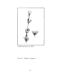 (copied from Hotchkiss 1967)
Figure 26. Nitella (Nftellas. sp,)
86
image:
(copied from Hotchkiss 1967)
Figure 26. Nitella (Nftellas. sp,)
86
image:
 size from 3 cm to 1.25 m tall. Many species form structures called bulbils
(Hutchinson 1975). Found on the rhizome,bulbils serve as anchors as well as
reproductive structures. Chara spp. are distinguished from the genera Nitella
and Tolypella mainly by the morphology of the apical crown on the oogonium
(Hutchinson 1975).
Reproduction. Characeae have highly specialized reproductive organization
(Fritsch 1965).Sexual reproduction usually occurs in the summer and autumn,
the photoperiod determining the ripening of the antheridia and oogonia (Migula
1909 cited in Hutchinson 1975). The germination of the oospores generally re-
quires from one to three months diapause in cold water (Proctor I960; Forsberg
1964, cited in Hutchinson 1975). Both sex organs are usually borne on secondary
leaves, originating from the nodes, with the oogonium directly above the anther-
idium (Fritsch 1965). Large numbers of motile sperm cells are produced by the
antheridia, fertilizing the oogonia through an opening at the top and producing
a resting spore (Schuette and Alder 1929aJ.
Chara reproduces asexually from bulbils and protonemata that arise from
the oospore and later from stem nodes (Hutchinson 1975). Hutchinson suggests
that asexual reproduction plays a major role in the species maintenance of the
Characeae.
Distribution
The Characeae constitute a group of primarily freshwater macrophytes that
forms a substantial part of the world's submerged vegetation in lakes, ponds
and streams (Cook et al. 1974). Chara species tend to inhabit hard or calcareous
waters and Nitella species generally inhabit soft or circumneutral water
(Hutchinson 1975). Inland saline lakes and ponds may be dominated by the
Characeae (Ungar 1974). Some species inhabit brackish waters but are not found
in truly marine environments (Hutchinson 1975) with various species found in
temperate and tropical regions of all the continents (Cook et al. 1974).
Since 1971, MBHRL has conducted an annual summer sampling program for sub-
merged aquatics in the Maryland portion of the Chesapeake Bay. Out of over 600
stations sampled each year, the survey has documented Characeae only in the
Susquehanna Flats and Magothy, Severn and Chester Rivers (see Figure 27). How-
ever, compared to Potamogeton spp. for example, Chara spp. showed a very low
rate of occurrence within the Maryland Bay portion. Chapter 3 discusses avail-
able historic data on the Characeae in the Chesapeake Bay.
Environmental Factors Affecting Distribution
Temperature. Temperature affects Characeae distribution through the regula-
tion of oospore germination. Maintenance at about 40 C for one to three months
was shown to be necessary to produce germination (Hutchinson 1975). Various
species within the Characeae persist throughout the year in temperate climates
and can even be found as green plants well below the ice layer (Flossner 1964,
cited in Hutchinson 1975).
Salinity. Though Characeae are predominantly freshwater inhabitants,
Dawson (1966) allocated about 13 percent of the known species to brackish waters
87
image:
size from 3 cm to 1.25 m tall. Many species form structures called bulbils
(Hutchinson 1975). Found on the rhizome,bulbils serve as anchors as well as
reproductive structures. Chara spp. are distinguished from the genera Nitella
and Tolypella mainly by the morphology of the apical crown on the oogonium
(Hutchinson 1975).
Reproduction. Characeae have highly specialized reproductive organization
(Fritsch 1965).Sexual reproduction usually occurs in the summer and autumn,
the photoperiod determining the ripening of the antheridia and oogonia (Migula
1909 cited in Hutchinson 1975). The germination of the oospores generally re-
quires from one to three months diapause in cold water (Proctor I960; Forsberg
1964, cited in Hutchinson 1975). Both sex organs are usually borne on secondary
leaves, originating from the nodes, with the oogonium directly above the anther-
idium (Fritsch 1965). Large numbers of motile sperm cells are produced by the
antheridia, fertilizing the oogonia through an opening at the top and producing
a resting spore (Schuette and Alder 1929aJ.
Chara reproduces asexually from bulbils and protonemata that arise from
the oospore and later from stem nodes (Hutchinson 1975). Hutchinson suggests
that asexual reproduction plays a major role in the species maintenance of the
Characeae.
Distribution
The Characeae constitute a group of primarily freshwater macrophytes that
forms a substantial part of the world's submerged vegetation in lakes, ponds
and streams (Cook et al. 1974). Chara species tend to inhabit hard or calcareous
waters and Nitella species generally inhabit soft or circumneutral water
(Hutchinson 1975). Inland saline lakes and ponds may be dominated by the
Characeae (Ungar 1974). Some species inhabit brackish waters but are not found
in truly marine environments (Hutchinson 1975) with various species found in
temperate and tropical regions of all the continents (Cook et al. 1974).
Since 1971, MBHRL has conducted an annual summer sampling program for sub-
merged aquatics in the Maryland portion of the Chesapeake Bay. Out of over 600
stations sampled each year, the survey has documented Characeae only in the
Susquehanna Flats and Magothy, Severn and Chester Rivers (see Figure 27). How-
ever, compared to Potamogeton spp. for example, Chara spp. showed a very low
rate of occurrence within the Maryland Bay portion. Chapter 3 discusses avail-
able historic data on the Characeae in the Chesapeake Bay.
Environmental Factors Affecting Distribution
Temperature. Temperature affects Characeae distribution through the regula-
tion of oospore germination. Maintenance at about 40 C for one to three months
was shown to be necessary to produce germination (Hutchinson 1975). Various
species within the Characeae persist throughout the year in temperate climates
and can even be found as green plants well below the ice layer (Flossner 1964,
cited in Hutchinson 1975).
Salinity. Though Characeae are predominantly freshwater inhabitants,
Dawson (1966) allocated about 13 percent of the known species to brackish waters
87
image:
 Figure 27.
1971-1976
Distribution of Chara sp. , Maryland Chesapeake Bay,
88
image:
Figure 27.
1971-1976
Distribution of Chara sp. , Maryland Chesapeake Bay,
88
image:
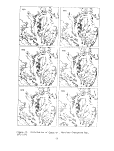 of coastal lagoons, ponds, coves and inland salt lakes and springs. Species
ranged in salinities up to 15 ppt with growth cessation and limited survival at
20 ppt.
Substrate. Most species of Characeae grow in silt or mud substrate though
a small number of species tend to grow in shallow water on sandy bottoms
(Hutchinson 1975). Studies in the Soviet Union (Zenkevitch 1963) uncovered
extensive Chareal growths on the shallow hydrogen sulfide silt soils of the
eastern coast of Russia. Further abundant growths have been documented in the
bays and inlets of the Soviet Aral Sea, growing on black ooze which smelled of
H2S.
Some species require not more than a few millimeters of soft deposits over
bedrock to insure survival (Hutchinson 1975).
Light, Depth and Turbidity. The Characeae are capable of surviving in low
light intensities, though none of the species are confined to such light inten-
sities in nature. Chara and Nitella species have often been found to grow
covered with calcium carbonate or mud deposits, respectively, which provided an
effective screen against solar radiation (Hutchinson 1975).
Characeae species can be found inhabiting transparent water well below the
limit of flowering plants. The greatest established depth for Chara spp. was
in Lake Tahoe at 65.5 m with incident radiation slightly more than 2 percent
of that reaching the lake surface (Hutchinson 1975).
The Charales are capable of existing with a small oxygen supply but require
pure water; they cannot tolerate turbid or contaminated conditions (Fritsch
1965).
Current Wind and Wave Action. Most of the Characeae are not conspicuous
littoral inhabitants, occupying instead the deep waters in lakes and some-
times running water (Hutchinson 1975).
Nutrient Response. Charophyceae are able to take up HC03" as an alternate
carbon source to C02 (Hutchinson 1975). Chara is known for its ability to
inhabit hard water. This may be related to the generally higher availability
of HC03~ in hard water and the ability of Chara to use the bicarbonate ion.
Anderson (1968) and Forsberg (1964, 1965), working with several different
species of Chara. determined that small excesses of phosphorus in the medium
inhibited growth. Experiments resulted in plant reduction but not destruction..
Optimum development occurred within a range of 5 to 20 mg total P/m~3.
As mentioned previously, Characeae can tolerate large amounts of free
H2S in bottom sediments. The green parts, however, are not as tolerant as are
the rhizomes, surviving for two weeks or more at only about 10 percent the H2S
tolerance level of the rhizomes (Hutchinson 1975).
Chara species have a high tolerance for photosynthetic CaC03 precipitates
(Hutchinson 1975). Calcium is essential to Chara, though requirements vary for
different species (Fritsch 1965).
89
image:
of coastal lagoons, ponds, coves and inland salt lakes and springs. Species
ranged in salinities up to 15 ppt with growth cessation and limited survival at
20 ppt.
Substrate. Most species of Characeae grow in silt or mud substrate though
a small number of species tend to grow in shallow water on sandy bottoms
(Hutchinson 1975). Studies in the Soviet Union (Zenkevitch 1963) uncovered
extensive Chareal growths on the shallow hydrogen sulfide silt soils of the
eastern coast of Russia. Further abundant growths have been documented in the
bays and inlets of the Soviet Aral Sea, growing on black ooze which smelled of
H2S.
Some species require not more than a few millimeters of soft deposits over
bedrock to insure survival (Hutchinson 1975).
Light, Depth and Turbidity. The Characeae are capable of surviving in low
light intensities, though none of the species are confined to such light inten-
sities in nature. Chara and Nitella species have often been found to grow
covered with calcium carbonate or mud deposits, respectively, which provided an
effective screen against solar radiation (Hutchinson 1975).
Characeae species can be found inhabiting transparent water well below the
limit of flowering plants. The greatest established depth for Chara spp. was
in Lake Tahoe at 65.5 m with incident radiation slightly more than 2 percent
of that reaching the lake surface (Hutchinson 1975).
The Charales are capable of existing with a small oxygen supply but require
pure water; they cannot tolerate turbid or contaminated conditions (Fritsch
1965).
Current Wind and Wave Action. Most of the Characeae are not conspicuous
littoral inhabitants, occupying instead the deep waters in lakes and some-
times running water (Hutchinson 1975).
Nutrient Response. Charophyceae are able to take up HC03" as an alternate
carbon source to C02 (Hutchinson 1975). Chara is known for its ability to
inhabit hard water. This may be related to the generally higher availability
of HC03~ in hard water and the ability of Chara to use the bicarbonate ion.
Anderson (1968) and Forsberg (1964, 1965), working with several different
species of Chara. determined that small excesses of phosphorus in the medium
inhibited growth. Experiments resulted in plant reduction but not destruction..
Optimum development occurred within a range of 5 to 20 mg total P/m~3.
As mentioned previously, Characeae can tolerate large amounts of free
H2S in bottom sediments. The green parts, however, are not as tolerant as are
the rhizomes, surviving for two weeks or more at only about 10 percent the H2S
tolerance level of the rhizomes (Hutchinson 1975).
Chara species have a high tolerance for photosynthetic CaC03 precipitates
(Hutchinson 1975). Calcium is essential to Chara, though requirements vary for
different species (Fritsch 1965).
89
image:
 Susceptibility. Experiments using the herbicides simazine, propazine and
atrazine in whole ponds in Missouri (Walker 1964) determined varied toxicity
results for Chara vulgaris. Propazine was the least effective herbicide, need-
ing a maximum application of 3.0 ppm (wettable powder) for only limited control.
Simazine and atrazine were slow to provide results. Simazine was applied at
rates ranging from 0.5 to 10.0 ppm and 5.5 to 132 kg/ha. Dry applications re-
sulted in zero control. Wet applications resulted in increasing control with
increasing concentration of herbicide, the maximum control being achieved at
10.0 ppm. Atrazine applications, corresponding to the simazine rates, resulted
in zero control of C_. vulgaris. Applications of herbicides during cold, cloudy
weather periods indicated that such weather did not favor the efficacy of the
chemicals. However, some limited growth inhibition did result from cold weather
applications.
Experimental work performed in Great Britain (Newbold 1975) recorded the
effects of eight herbicides approved by the Pesticide Safety Precautions Scheme
for use in or near water. Dichlobenil and chlorthiamid were found to be the
most effective, resulting in a 2-year kill of Chara spp. Terbutryne resulted
in a one-year kill and diquat and paraquat resulted inan initial kill, but re-
vegetation occurred within the same year. Applications of dalapon, dalapon-
paraquat and 2,4-D were not recommended for use and considered likely to be
inefficient.
Consumer Utilization
The Characeae are of considerable economic value and have been used for
water purification, as food for farm stock and fish stock, as an agent in
settling silt and in the manufacture of polishes (Cook et al. 1974). Many
species of ducks feed exclusively on Charophyceae while some species feed solely
on the bulbils (Hutchinson 1975).
By forming often times vast bottom meadows, the Characeae provide habitat
for aquatic fauna plus support for many lesser epiphytes (Needham and Lloyd
1930). According to Fassett (1960), Chara provides fair shelter and an excell-
ent source of fish food, especially for juvenile trout and large mouth and
small black bass.
Martin and Uhler (1939) studied aquatic plant usage by game ducks in
various areas of the United States and Canada. Based on volumetric percentage
of stomach materials, the study rated Characeae as having good to excellent
usage, the plants being consumed by many kinds of waterfowl, especially diving
ducks. All parts of the plants were discovered in duck stomachs, especially
the oogonia and bulbils.
Cottam (1939) studied the contents of gizzards and gullets from approxi-
mately 3,500 inland plant-feeding ducks in North America. Along with the pond-
weed family, Chara spp. was included in the list of submerged aquatics having
greatest value to Nyroca spp. and ruddy ducks. The study revealed that the
ducks were utilizing all parts of the plants: seeds, rhizomes, leaves and
bilbils.
90
image:
Susceptibility. Experiments using the herbicides simazine, propazine and
atrazine in whole ponds in Missouri (Walker 1964) determined varied toxicity
results for Chara vulgaris. Propazine was the least effective herbicide, need-
ing a maximum application of 3.0 ppm (wettable powder) for only limited control.
Simazine and atrazine were slow to provide results. Simazine was applied at
rates ranging from 0.5 to 10.0 ppm and 5.5 to 132 kg/ha. Dry applications re-
sulted in zero control. Wet applications resulted in increasing control with
increasing concentration of herbicide, the maximum control being achieved at
10.0 ppm. Atrazine applications, corresponding to the simazine rates, resulted
in zero control of C_. vulgaris. Applications of herbicides during cold, cloudy
weather periods indicated that such weather did not favor the efficacy of the
chemicals. However, some limited growth inhibition did result from cold weather
applications.
Experimental work performed in Great Britain (Newbold 1975) recorded the
effects of eight herbicides approved by the Pesticide Safety Precautions Scheme
for use in or near water. Dichlobenil and chlorthiamid were found to be the
most effective, resulting in a 2-year kill of Chara spp. Terbutryne resulted
in a one-year kill and diquat and paraquat resulted inan initial kill, but re-
vegetation occurred within the same year. Applications of dalapon, dalapon-
paraquat and 2,4-D were not recommended for use and considered likely to be
inefficient.
Consumer Utilization
The Characeae are of considerable economic value and have been used for
water purification, as food for farm stock and fish stock, as an agent in
settling silt and in the manufacture of polishes (Cook et al. 1974). Many
species of ducks feed exclusively on Charophyceae while some species feed solely
on the bulbils (Hutchinson 1975).
By forming often times vast bottom meadows, the Characeae provide habitat
for aquatic fauna plus support for many lesser epiphytes (Needham and Lloyd
1930). According to Fassett (1960), Chara provides fair shelter and an excell-
ent source of fish food, especially for juvenile trout and large mouth and
small black bass.
Martin and Uhler (1939) studied aquatic plant usage by game ducks in
various areas of the United States and Canada. Based on volumetric percentage
of stomach materials, the study rated Characeae as having good to excellent
usage, the plants being consumed by many kinds of waterfowl, especially diving
ducks. All parts of the plants were discovered in duck stomachs, especially
the oogonia and bulbils.
Cottam (1939) studied the contents of gizzards and gullets from approxi-
mately 3,500 inland plant-feeding ducks in North America. Along with the pond-
weed family, Chara spp. was included in the list of submerged aquatics having
greatest value to Nyroca spp. and ruddy ducks. The study revealed that the
ducks were utilizing all parts of the plants: seeds, rhizomes, leaves and
bilbils.
90
image:
 Economic Uses and Problems
Impoundments^ Chara has been utilized in southeast U.S. as waterfowl food
in shallow fresh water lakes and ponds (Ball 1965). However, beneficial results
were found to be temporary unless extensive management procedures were used to
prevent natural plant succession and invasion of pest plants.
Impacts to Mosquitoes. Hutchinson (1975) cited experimental work performed
in numerous countries on the effects of Chara and Mi tell a on mosquitoes. Ex-
perimental evidence implicated various Chara species as having possible larvici-
dal properties and egg laying inhibitors. Hutchinson expressed the need for
experimental determination of the possibility of using native species of Chara
and Nitella for mosquito control.
CERATOPHYLLUM DEMERSUM
Biology
General Vegetative Morphology. Known variously as hornwort or coontail,
Ceratophyllum demersum is a variable, cosmopolitan species of the family
Ceratophyllaceae. Found primarily in the still or slow moving waters of streams
and ponds, £. demersum is rootless (Steward et al. 1960; Fasset 1960). Coontail
may form large masses that drift just below the water surface (Mitchell 1974).
Capable of extreme reproductive growth, £. demersum was first recorded in a New
Zealand lake in 1963 and two years later caused the closure of a power station
after large mats of coontail had completely blocked the turbine screens (Chapman
et al. 1974).
Hornwort is exceedingly variable in form and foliage toothing. In general,
the leaves are divided into filiform or linear segments that are sparsely forked,
minutely denticulate with 9 to 10 leaves to a whorl (see Figure 28). Stems are
densely branched, up to 3 m in length, slender and extremely fragile. Flowers
are generally small and monoecious, with staminate flowers usuallyborne in pairs
on either side of a leaf axil and pistilate flowers solitary in leaf axial, both
usually found at different nodes (Mason 1969; Sculthorpe 1967).
As one of the primary colonizers in aquatic ecosystems, £. demersum is in-
cluded by Mitchell (1974) among a group of macrophytes characterized by the
following:
• capable of rapid vegetative growth;
• able to regenerate from small vegetative portions;
• partially independent from structures of sexual reproduction;
• attains large areas of photosynthetic tissue through vegetative
growth; and
• independent of water level fluctuations and bottom substrate.
91
image:
Economic Uses and Problems
Impoundments^ Chara has been utilized in southeast U.S. as waterfowl food
in shallow fresh water lakes and ponds (Ball 1965). However, beneficial results
were found to be temporary unless extensive management procedures were used to
prevent natural plant succession and invasion of pest plants.
Impacts to Mosquitoes. Hutchinson (1975) cited experimental work performed
in numerous countries on the effects of Chara and Mi tell a on mosquitoes. Ex-
perimental evidence implicated various Chara species as having possible larvici-
dal properties and egg laying inhibitors. Hutchinson expressed the need for
experimental determination of the possibility of using native species of Chara
and Nitella for mosquito control.
CERATOPHYLLUM DEMERSUM
Biology
General Vegetative Morphology. Known variously as hornwort or coontail,
Ceratophyllum demersum is a variable, cosmopolitan species of the family
Ceratophyllaceae. Found primarily in the still or slow moving waters of streams
and ponds, £. demersum is rootless (Steward et al. 1960; Fasset 1960). Coontail
may form large masses that drift just below the water surface (Mitchell 1974).
Capable of extreme reproductive growth, £. demersum was first recorded in a New
Zealand lake in 1963 and two years later caused the closure of a power station
after large mats of coontail had completely blocked the turbine screens (Chapman
et al. 1974).
Hornwort is exceedingly variable in form and foliage toothing. In general,
the leaves are divided into filiform or linear segments that are sparsely forked,
minutely denticulate with 9 to 10 leaves to a whorl (see Figure 28). Stems are
densely branched, up to 3 m in length, slender and extremely fragile. Flowers
are generally small and monoecious, with staminate flowers usuallyborne in pairs
on either side of a leaf axil and pistilate flowers solitary in leaf axial, both
usually found at different nodes (Mason 1969; Sculthorpe 1967).
As one of the primary colonizers in aquatic ecosystems, £. demersum is in-
cluded by Mitchell (1974) among a group of macrophytes characterized by the
following:
• capable of rapid vegetative growth;
• able to regenerate from small vegetative portions;
• partially independent from structures of sexual reproduction;
• attains large areas of photosynthetic tissue through vegetative
growth; and
• independent of water level fluctuations and bottom substrate.
91
image:
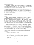 (copied from Hotchkiss 1967)
Figure 28. Coontail (CeratophyTlum denier sum)
92
image:
(copied from Hotchkiss 1967)
Figure 28. Coontail (CeratophyTlum denier sum)
92
image:
 Reproduction. Ceratophyllum demersum reproduces mainly through vegetative
means. Almost any fragment of stem bearing a lateral bud is capable of forming
a new plant, Sexual reproduction occurs when the mature anther reaches the
surface, dehisces and releases microspores which sink down slowly to the female
flower (Sculthorpe 1967). Fertilization produces a one-seeded nutlet which
needs to remain in the water in order to germinate. Experiments by Muenscher
(1936) indicated that once seeds were dried, no germination would occur.
Distribution
Ceratophyllum demersum is considered to be truly cosmopolitan exhibiting
remarkable latitude penetration. Fossil records show hornwort to be well re-
presented in Pliocene deposits at Castle Eden and Palsefield in Suffolk
(Sculthorpe 1967). Worldwide, coontail frequents quiet, fresh water pools and
slow streams (Mason 1969). Fragments of Ceratophyllurn are frequently transported
casually when caught in waterfowl feathers (Sculthorpe 1967).
MBHRL Survey work from 1971 to 1976 has documented £. demersum as sparse
and limited primarily to the Susquehanna Flats, Magothy, Severn and Chester
Rivers (see Figure 29). Chapter 3 includes available data by river system per-
taining to historic distribution of hornwort in the Maryland portion of the
Chesapeake Bay.
Environmental Factors Effecting Distribution
Temperature. Fruit maturation of C. demersum seems to require almost
tropical temperature conditions, thus limiting sexual reproduction mainly to
warm climates (Martin and Uhler 1939). Wilkinson (1963) determined a critical
minimum temperature for vegetative growth of 20 C with optimum growth at 30 C.
Salinity. Ceratophyllum demersum is essentially a fresh water macrophyte
(Martin and Uhler 1939). Salinity experiments (Bourn 1932) conducted under
favorable soil, C02, light and temperature conditions resulted in growth retar-
dation of Ceratophyllum with increasing concentrations of salinity. Based on
percentage increase in dry weight, Ceratophyllum decreased in growth roughly
proportional to the increase in salinity. However, plants appeared to develop
normally in salinities under 6.5 ppt. Above 6.5 ppt, plants showed size red-
uction, spindly stems and curling leaves. An endurance limit was established at
about 8 ppt.
Substrate. Hornwort often grows independently of substrate material. Ac-
cording to experiments by Shannon (1953), Ceratophyllum showed no capability
for root production even when grown in wet sand or wet sphagnum. However,
when C^. demersum plants were suspended over sand or mud, the plants grown over
mud produced a mean crop that was twice that produced over sand (Hutchinson 1975),
Though available literature refers to Ceratophyllum as being rootless
(Sculthorpe 1967), there appears to be some question as to whether C_. demersum
is always rootless in the Cheapeake Bay. Stotts (personal communication) has
found hornwort in the Bay that has been rooted. This may be due to the location
of the Bay in a temperature transition zone for Ceratophyllum. The Bay has both
93
image:
Reproduction. Ceratophyllum demersum reproduces mainly through vegetative
means. Almost any fragment of stem bearing a lateral bud is capable of forming
a new plant, Sexual reproduction occurs when the mature anther reaches the
surface, dehisces and releases microspores which sink down slowly to the female
flower (Sculthorpe 1967). Fertilization produces a one-seeded nutlet which
needs to remain in the water in order to germinate. Experiments by Muenscher
(1936) indicated that once seeds were dried, no germination would occur.
Distribution
Ceratophyllum demersum is considered to be truly cosmopolitan exhibiting
remarkable latitude penetration. Fossil records show hornwort to be well re-
presented in Pliocene deposits at Castle Eden and Palsefield in Suffolk
(Sculthorpe 1967). Worldwide, coontail frequents quiet, fresh water pools and
slow streams (Mason 1969). Fragments of Ceratophyllurn are frequently transported
casually when caught in waterfowl feathers (Sculthorpe 1967).
MBHRL Survey work from 1971 to 1976 has documented £. demersum as sparse
and limited primarily to the Susquehanna Flats, Magothy, Severn and Chester
Rivers (see Figure 29). Chapter 3 includes available data by river system per-
taining to historic distribution of hornwort in the Maryland portion of the
Chesapeake Bay.
Environmental Factors Effecting Distribution
Temperature. Fruit maturation of C. demersum seems to require almost
tropical temperature conditions, thus limiting sexual reproduction mainly to
warm climates (Martin and Uhler 1939). Wilkinson (1963) determined a critical
minimum temperature for vegetative growth of 20 C with optimum growth at 30 C.
Salinity. Ceratophyllum demersum is essentially a fresh water macrophyte
(Martin and Uhler 1939). Salinity experiments (Bourn 1932) conducted under
favorable soil, C02, light and temperature conditions resulted in growth retar-
dation of Ceratophyllum with increasing concentrations of salinity. Based on
percentage increase in dry weight, Ceratophyllum decreased in growth roughly
proportional to the increase in salinity. However, plants appeared to develop
normally in salinities under 6.5 ppt. Above 6.5 ppt, plants showed size red-
uction, spindly stems and curling leaves. An endurance limit was established at
about 8 ppt.
Substrate. Hornwort often grows independently of substrate material. Ac-
cording to experiments by Shannon (1953), Ceratophyllum showed no capability
for root production even when grown in wet sand or wet sphagnum. However,
when C^. demersum plants were suspended over sand or mud, the plants grown over
mud produced a mean crop that was twice that produced over sand (Hutchinson 1975),
Though available literature refers to Ceratophyllum as being rootless
(Sculthorpe 1967), there appears to be some question as to whether C_. demersum
is always rootless in the Cheapeake Bay. Stotts (personal communication) has
found hornwort in the Bay that has been rooted. This may be due to the location
of the Bay in a temperature transition zone for Ceratophyllum. The Bay has both
93
image:
 1971
1973
1975
1972
1974
1976
Figure 29. Distribution of Ceratophyllum demersum, Maryland Chesapeake
Bay, 1971-1976 ~~
94
image:
1971
1973
1975
1972
1974
1976
Figure 29. Distribution of Ceratophyllum demersum, Maryland Chesapeake
Bay, 1971-1976 ~~
94
image:
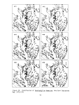 sheltered areas with higher ambient temperatures possibly more conducive to sexual
reproduction and more exposed areas with lower mean temperatures where vegetative
growth could be favored (Confer, personal communication).
Light, Depth and Turbidity. Coontail is shade tolerant (Lamoureux 1957)
requiring a minimum of 2 percent full sunlight for optimum growth (Chapman et al.
1974). Experiments conducted in an Ohio Lake (Meyer et al. 1943) concluded
that C_. demersum reached a compensation point of zero photosynthesis at less
2 percent full sunlight intensity. In Back Bay and Currituck Sound, C_. demersum
was found thriving in the dark brown water draining from the swamps (Bourn 1932).
Coontail is sufficiently shade tolerant to exist under floating leaved plants
(Lind and Cottam 1969).
Ceratophyllum generally is not considered to be depth limited due to its
often rootless nature. Turbidity is not as negative a factor for coontail as
for rooted aquatics due to shade tolerance and water surface habitat.
Current Hind and Wave Action. Ceratophyllum demersum is sensitive to
current,wind and wave action (Mitchell 1974).Any violent disturbance has been
found to break the fragile stems (Sculthorpe 1967). However, this does not re-
sult in mortality but instead acts in dispersal and increased vegetative growth.
Nutrient Response. Ceratophyllum absorbs necessary nutrients from water
rather than soil media (Sculthorpe 1967). Toetz (1973) suggested that for
Ceratophyllum, dissolved NH^ input from sediments, animal excretion, autolysis
and microbial decomposition might have been the ultimate limiting factor in
waters with an immense biomass. Table 13 lists several other elements found to
concentrate in Ceratophyllum.
Table 13. Concentration factors for Ceratophyllum demersum9
Mean Mean
Element concentration concentration Concentration
water dry plant factor
(mg/r1) (ppm x 0.1)
Cooper .0160 3.23 202
.0083 1.52 183
Zinc .0090 16.40 1820
Cadmium .0015b 9.12b 600 to 700
aHutchinson 1975
Value in ppm
95
image:
sheltered areas with higher ambient temperatures possibly more conducive to sexual
reproduction and more exposed areas with lower mean temperatures where vegetative
growth could be favored (Confer, personal communication).
Light, Depth and Turbidity. Coontail is shade tolerant (Lamoureux 1957)
requiring a minimum of 2 percent full sunlight for optimum growth (Chapman et al.
1974). Experiments conducted in an Ohio Lake (Meyer et al. 1943) concluded
that C_. demersum reached a compensation point of zero photosynthesis at less
2 percent full sunlight intensity. In Back Bay and Currituck Sound, C_. demersum
was found thriving in the dark brown water draining from the swamps (Bourn 1932).
Coontail is sufficiently shade tolerant to exist under floating leaved plants
(Lind and Cottam 1969).
Ceratophyllum generally is not considered to be depth limited due to its
often rootless nature. Turbidity is not as negative a factor for coontail as
for rooted aquatics due to shade tolerance and water surface habitat.
Current Hind and Wave Action. Ceratophyllum demersum is sensitive to
current,wind and wave action (Mitchell 1974).Any violent disturbance has been
found to break the fragile stems (Sculthorpe 1967). However, this does not re-
sult in mortality but instead acts in dispersal and increased vegetative growth.
Nutrient Response. Ceratophyllum absorbs necessary nutrients from water
rather than soil media (Sculthorpe 1967). Toetz (1973) suggested that for
Ceratophyllum, dissolved NH^ input from sediments, animal excretion, autolysis
and microbial decomposition might have been the ultimate limiting factor in
waters with an immense biomass. Table 13 lists several other elements found to
concentrate in Ceratophyllum.
Table 13. Concentration factors for Ceratophyllum demersum9
Mean Mean
Element concentration concentration Concentration
water dry plant factor
(mg/r1) (ppm x 0.1)
Cooper .0160 3.23 202
.0083 1.52 183
Zinc .0090 16.40 1820
Cadmium .0015b 9.12b 600 to 700
aHutchinson 1975
Value in ppm
95
image:
 Susceptibility. Ceratophyllum has been shown to be highly resistant to
large concentrations of boron. Boron is even stimulatory to photosynthesis
within a range of 0.5 to 100 mg/1. Greater concentrations were found to affect
protein synthesis, water balance and nutrient assimilation (Wetzel 1964). In
normal water, arsenic has been found to accumulate in C. demersum up to 26 ppm.
In geothermal waters in New Zealand coontail has been recorded to contain 1,000
ppm arsenic as dry material (Hutchinson 1975).
Attempts to eradicate Certophyl'lum demersum have been well documented.
Table 14 lists various herbicides and related application rates and control
results.
Various fauna are known to consume £. demersum including Chinese grass carp
or white amur (Ctenopharyngodon idella). The Brazilian snail (Marisa cornvarietis)
also consumes coontail; however, research into the use of these snails for con-
trol of Ceratophyllum has shown that such action would probably disturb the
entire ecosystem (Chapman et al. 1974).
Productivity
As has been previously mentioned, £. demersum is highly productive through
vegetative means. Any fragment that includes a bud is capable of producing a
new plant. Chapman et al. (1974) found high photosynthesis rates in these
apical buds plus in relatively new leaves. Stems and older leaves produced con-
siderably lower amounts of oxygen.
Consumer Utilization
Ceratophyllum demersum is not unanimously considered to be of great impor-
tance to wildlife. Cottam (1939) did not include coontail in his listing of
aquatic macrophytes having great value to Nyroca and ruddy ducks. Lamoureux
(1957) rated Ceratophyllum as slightly important as duck food with seeds and
leaves eaten only occasionally. Sculthorpe (1967), however, rated foliage and
seeds as having great food importance to ducks, coots, geese, grebes, swans,
waders, shore and game birds. Ceratophyllum foliage has further moderate impor-
tance as fish food. As a shade, shelter and spawning medium, Sculthorpe rated
coontail high. The dissected leaves of Ceratophyllum may support dense com-
munities of epiphytic desmids, diatoms, filamentous algae and zooplankton
which all provide food for fish.
On a somewhat different note, preparations of leaves have historically
been used internally as purgatives and diuretics, for dysentery and as remedies
for bilousness and jaundice. Topically, leaf extracts have been used to treat
anything from elephantiasis to sunburn (Sculthorpe, 1967).
96
image:
Susceptibility. Ceratophyllum has been shown to be highly resistant to
large concentrations of boron. Boron is even stimulatory to photosynthesis
within a range of 0.5 to 100 mg/1. Greater concentrations were found to affect
protein synthesis, water balance and nutrient assimilation (Wetzel 1964). In
normal water, arsenic has been found to accumulate in C. demersum up to 26 ppm.
In geothermal waters in New Zealand coontail has been recorded to contain 1,000
ppm arsenic as dry material (Hutchinson 1975).
Attempts to eradicate Certophyl'lum demersum have been well documented.
Table 14 lists various herbicides and related application rates and control
results.
Various fauna are known to consume £. demersum including Chinese grass carp
or white amur (Ctenopharyngodon idella). The Brazilian snail (Marisa cornvarietis)
also consumes coontail; however, research into the use of these snails for con-
trol of Ceratophyllum has shown that such action would probably disturb the
entire ecosystem (Chapman et al. 1974).
Productivity
As has been previously mentioned, £. demersum is highly productive through
vegetative means. Any fragment that includes a bud is capable of producing a
new plant. Chapman et al. (1974) found high photosynthesis rates in these
apical buds plus in relatively new leaves. Stems and older leaves produced con-
siderably lower amounts of oxygen.
Consumer Utilization
Ceratophyllum demersum is not unanimously considered to be of great impor-
tance to wildlife. Cottam (1939) did not include coontail in his listing of
aquatic macrophytes having great value to Nyroca and ruddy ducks. Lamoureux
(1957) rated Ceratophyllum as slightly important as duck food with seeds and
leaves eaten only occasionally. Sculthorpe (1967), however, rated foliage and
seeds as having great food importance to ducks, coots, geese, grebes, swans,
waders, shore and game birds. Ceratophyllum foliage has further moderate impor-
tance as fish food. As a shade, shelter and spawning medium, Sculthorpe rated
coontail high. The dissected leaves of Ceratophyllum may support dense com-
munities of epiphytic desmids, diatoms, filamentous algae and zooplankton
which all provide food for fish.
On a somewhat different note, preparations of leaves have historically
been used internally as purgatives and diuretics, for dysentery and as remedies
for bilousness and jaundice. Topically, leaf extracts have been used to treat
anything from elephantiasis to sunburn (Sculthorpe, 1967).
96
image:
 Table 14. Effects of certain herbicides on Ceratophy11 urn demersum
Herbicide
Application rate
Control
Silvex, K salt
Diquat dibromide
Diquat
Paraquat
Ipazine
Acrolein
Endothall
Endothall DOS
2,4,-D
Ametryne
Sodium arsenite
Simazine
Atrazine
1.5 to 2 ppm
22 kg/ha granules
1 to 2.5 ppm
5 to 10 ppm
5 ppm
1 to 2.5 ppm
5 to 10 ppm
1 to 2.5 ppm
5 to 10 ppm
1 to 2.5 ppm
5 to 10 ppm
1 ppm
2 to 3 ppm
16.5 to 33 kg/ha granules
5 ppm granules
1 to 5 ppm
3 ppm
33 kg/ha granules
4 to 5 ppm
1 to 2 ppm
7 to 10 ppm
10 to 20 ppm bottom granules
5 to 6 ppm wettable powder
6 ppm granules
5 to 6 ppm wettable powder
5 to 6 ppm granules
100%
100% initial kill with regrowth
75 - 80% after 24 hours
89 - 100% after 24 hours
Satisfactory
50 - 65% after 24 hours
90 - 97% after 24 hours
0 - 5% after 24 hours
10% after 24 hours
79 - 95% after 24 hours
99 - 100% after 24 hours
Poor
For Season
None
Effective
Good
Good
Good
Good
90%
Killed within one week
Unsatisfactory
Erratic
Satisfactory
Erratic
Satisfactory
Source: Lawrence and Hollingsworth 1969.
97
image:
Table 14. Effects of certain herbicides on Ceratophy11 urn demersum
Herbicide
Application rate
Control
Silvex, K salt
Diquat dibromide
Diquat
Paraquat
Ipazine
Acrolein
Endothall
Endothall DOS
2,4,-D
Ametryne
Sodium arsenite
Simazine
Atrazine
1.5 to 2 ppm
22 kg/ha granules
1 to 2.5 ppm
5 to 10 ppm
5 ppm
1 to 2.5 ppm
5 to 10 ppm
1 to 2.5 ppm
5 to 10 ppm
1 to 2.5 ppm
5 to 10 ppm
1 ppm
2 to 3 ppm
16.5 to 33 kg/ha granules
5 ppm granules
1 to 5 ppm
3 ppm
33 kg/ha granules
4 to 5 ppm
1 to 2 ppm
7 to 10 ppm
10 to 20 ppm bottom granules
5 to 6 ppm wettable powder
6 ppm granules
5 to 6 ppm wettable powder
5 to 6 ppm granules
100%
100% initial kill with regrowth
75 - 80% after 24 hours
89 - 100% after 24 hours
Satisfactory
50 - 65% after 24 hours
90 - 97% after 24 hours
0 - 5% after 24 hours
10% after 24 hours
79 - 95% after 24 hours
99 - 100% after 24 hours
Poor
For Season
None
Effective
Good
Good
Good
Good
90%
Killed within one week
Unsatisfactory
Erratic
Satisfactory
Erratic
Satisfactory
Source: Lawrence and Hollingsworth 1969.
97
image:
 NAJAS GUADALUPENSIS
Biology
General Vegetative Morphology. Najas guadalupensis is commonly referred
to as bushy pondweed (Radford et al. 1964) or water nymph (Schuette and Alder
1929b). Physically resembling Zannichellia and Elodea, Najas is the single genus
of the Najadaceae family. Members of the genus are either monoecious or dioecious,
annual or perennial and have slender branched stems with simple, linear, opposite
leaves that are often marginally toothed and have sheathed bases (See Figure 30)
(Cook et al. 1974).
Around the turn of the century there appears to have been a rather heated
debate among several reknowned botanists regarding the primitive or advanced
nature of Najas. Rendle (1899, cited in Arbor 1920) maintained that Najas
was a primitive monocotyledon. Guppy's "Differentiation Theory" also
categorized Najas as a primitive species. He maintained that N. marina had
evolved into other distinct species within the same genus since N. marina ex-
hibited a wider range than other species of Najas. Arbor (1920) disagreed with
both Rendle and Guppy, stating that the genus Najas was a "highly reduced form
representing perhaps the ultimate term of reduction in the Potamogetonaceae
series." Schuette and Alder (1929), some years after the previous controversy,
referred to Najas as appearing to be a primitive monocotyledon.
There appears to be further confusion in literature regarding whether
Najas spp. are annual or perennial. Radford et al. (1964) and Hutchinson (1975)
refer to the genus as annual. Arbor (1920), however, cites only the species
N. minor and N. flexibis as being annuals. Cook et al. (1974) leaves the choice
open for individual species and simply lists the genus as either annual or
perennial. Information as to which group N. guadalupensis fits in is not readily
available.
Najas spp. do not have rhizomes or tubers as do most other species of SAV
(U.S. Department of the Interior 1944). Roots are simple and small with a
radicle that is either short-lived or undeveloped (Arbor 1920; Bourn 1932).
Reproduction. Najas spp. appear to reproduce primarily sexually. Pollina-
tion takes place underwater (Hutchinson 1975) as the globular or elipsoid micro-
spores float up through the water and are caught on the elongated stigmas
(Schulthorpe 1967). The female flower consists of a single ovule that sometimes
is surrounded by one or two envelopes, evidently depending on the species
(Arbor 1920).
Vegetative reproduction does not appear to be as common or successful as
sexual reproduction. In discussing attempts to propagate Najas sp., the U.S.
Department of Interior (1944) suggested propagation by whole plants or seeds.
Vegetation by cuttings seemed to require a specimen with at least three nodes.
Distribution. Najas is essentially a freshwater species that ranges in
habitat from Oregon to Quebec and from California to Florida (Hotchkiss 1967).
Martin and Uhler (1939) considered Najas guadalupensis as a fresh or mildly
brackish water species.
98
image:
NAJAS GUADALUPENSIS
Biology
General Vegetative Morphology. Najas guadalupensis is commonly referred
to as bushy pondweed (Radford et al. 1964) or water nymph (Schuette and Alder
1929b). Physically resembling Zannichellia and Elodea, Najas is the single genus
of the Najadaceae family. Members of the genus are either monoecious or dioecious,
annual or perennial and have slender branched stems with simple, linear, opposite
leaves that are often marginally toothed and have sheathed bases (See Figure 30)
(Cook et al. 1974).
Around the turn of the century there appears to have been a rather heated
debate among several reknowned botanists regarding the primitive or advanced
nature of Najas. Rendle (1899, cited in Arbor 1920) maintained that Najas
was a primitive monocotyledon. Guppy's "Differentiation Theory" also
categorized Najas as a primitive species. He maintained that N. marina had
evolved into other distinct species within the same genus since N. marina ex-
hibited a wider range than other species of Najas. Arbor (1920) disagreed with
both Rendle and Guppy, stating that the genus Najas was a "highly reduced form
representing perhaps the ultimate term of reduction in the Potamogetonaceae
series." Schuette and Alder (1929), some years after the previous controversy,
referred to Najas as appearing to be a primitive monocotyledon.
There appears to be further confusion in literature regarding whether
Najas spp. are annual or perennial. Radford et al. (1964) and Hutchinson (1975)
refer to the genus as annual. Arbor (1920), however, cites only the species
N. minor and N. flexibis as being annuals. Cook et al. (1974) leaves the choice
open for individual species and simply lists the genus as either annual or
perennial. Information as to which group N. guadalupensis fits in is not readily
available.
Najas spp. do not have rhizomes or tubers as do most other species of SAV
(U.S. Department of the Interior 1944). Roots are simple and small with a
radicle that is either short-lived or undeveloped (Arbor 1920; Bourn 1932).
Reproduction. Najas spp. appear to reproduce primarily sexually. Pollina-
tion takes place underwater (Hutchinson 1975) as the globular or elipsoid micro-
spores float up through the water and are caught on the elongated stigmas
(Schulthorpe 1967). The female flower consists of a single ovule that sometimes
is surrounded by one or two envelopes, evidently depending on the species
(Arbor 1920).
Vegetative reproduction does not appear to be as common or successful as
sexual reproduction. In discussing attempts to propagate Najas sp., the U.S.
Department of Interior (1944) suggested propagation by whole plants or seeds.
Vegetation by cuttings seemed to require a specimen with at least three nodes.
Distribution. Najas is essentially a freshwater species that ranges in
habitat from Oregon to Quebec and from California to Florida (Hotchkiss 1967).
Martin and Uhler (1939) considered Najas guadalupensis as a fresh or mildly
brackish water species.
98
image:
 (redrawn after Hotchkiss 1967)
Figure 30. Naiad (Najas sp.)
99
image:
(redrawn after Hotchkiss 1967)
Figure 30. Naiad (Najas sp.)
99
image:
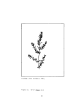 Distribution of NL guadalupensis in the Maryland portion of the Chesapeake
Bay presently appears to be limited to the Chester River (see Figure 31).
Historically, Najas was once abundant on the Susquehanna Flats. The Susquehanna
Flats Survey (1958 to 1975) documented Najas through 1971. Then Najas suddenly
disappeared and neither the Susquehanna Flats or MBHRL survey teams found Najas
in the area until 1977 when the Flats survey teams documented N_. guadalupensis
as "rare" (Stotts, personal communication).
Environmental Factors Affecting Distribution
Salinity. According to Steenis'(1970), Najas prefers a salinity of 3 ppt.
Haller et al. (1974) concluded from experiments that N^. guadalupensis died
after four weeks at 10 ppt. Growth experiments based on g/dry weight measure-
ments resulted in maximum growth at 0.17 ppt with decreasing growth in increasing
salinities. Martin and Uhler (1939) found N_. guadalupens in the Potomac River
growing in salinities from about 6 to 9 ppt.
Substrate. U.S. Department of Interior (1944) and Martin and Uhler (1939)
agreed that Najas thrived best in soils containing a predominance of sand though
the species has been found growing on almost pure muck. USDI added that firmer
substrates appeared to be preferred.
Light. Depth and Turbidity. U.S. Department of Interior (1944) stated
that Najas sp. required less light than most other species of SAV. Martin
a-nd Uhler (1939) added that Najas sp. was usually found in depths ranging from
0.3 to 1.2 m but could be found locally at depths over 6 m. Seed germination
appears to be affected by light intensity. Hutchinson (1975) described germina-
tion of NL marina and N_. flexilis as being inhibited by light.
Nutrient Responses. Najas guadalupensis growth does not appear to be re-
la ted^tb^eltheTliiltrogFn or phosphorous levels (Peltier and Welch 1969).
Currents and Wave Action. Martin and Uhler (1939) found N_. guadalupensis
growing in areas with retarded currents but only if sedimentation was not
extreme.
Susceptibility. The destruction of aquatic vegetation in Back Bay/Currituck
Sound around 1929 provided a situation for the study of environmental factors
affecting SAV growth. Najas sp. was found to be intolerant of extreme turbidity
and varying salinity (Martin and Uhler 1939). It was also concluded that
negative impacts to Najas occurred due to the brackish water hydroid Cordylophora
lacustris and the fungus Rhizoctom'a sol am' (Martin and Uhler 1939). Crawfish
Cambarus rusticus) was found tocontrol Najas sp. in the lower Ohio River and its
tributaries (Martin and Uhler 1939). Smothering by benthic algae was also found
to be a successful method of control (Sculthorpel967). Mitchell (1974) listed
the marisa snail (Schistosoma mansoni) as providing seasonal control. Grass
carp feed on young Najas stems and leaves along with Potamogeton sp. and El odea
sp. though established, mature growth was not controlled. In discussing the
grass carp (Ctenopharyngodon idell us), the Avauet (1965) concluded that the carp
could effect complete control of j\L guadalupensis after two to three weeks in
experimental plastic pools. Seaman and Porterfield (1964) found complete control
of IN. guadalupensis by the fresh water snail Marisa cornuarietis.
100
image:
Distribution of NL guadalupensis in the Maryland portion of the Chesapeake
Bay presently appears to be limited to the Chester River (see Figure 31).
Historically, Najas was once abundant on the Susquehanna Flats. The Susquehanna
Flats Survey (1958 to 1975) documented Najas through 1971. Then Najas suddenly
disappeared and neither the Susquehanna Flats or MBHRL survey teams found Najas
in the area until 1977 when the Flats survey teams documented N_. guadalupensis
as "rare" (Stotts, personal communication).
Environmental Factors Affecting Distribution
Salinity. According to Steenis'(1970), Najas prefers a salinity of 3 ppt.
Haller et al. (1974) concluded from experiments that N^. guadalupensis died
after four weeks at 10 ppt. Growth experiments based on g/dry weight measure-
ments resulted in maximum growth at 0.17 ppt with decreasing growth in increasing
salinities. Martin and Uhler (1939) found N_. guadalupens in the Potomac River
growing in salinities from about 6 to 9 ppt.
Substrate. U.S. Department of Interior (1944) and Martin and Uhler (1939)
agreed that Najas thrived best in soils containing a predominance of sand though
the species has been found growing on almost pure muck. USDI added that firmer
substrates appeared to be preferred.
Light. Depth and Turbidity. U.S. Department of Interior (1944) stated
that Najas sp. required less light than most other species of SAV. Martin
a-nd Uhler (1939) added that Najas sp. was usually found in depths ranging from
0.3 to 1.2 m but could be found locally at depths over 6 m. Seed germination
appears to be affected by light intensity. Hutchinson (1975) described germina-
tion of NL marina and N_. flexilis as being inhibited by light.
Nutrient Responses. Najas guadalupensis growth does not appear to be re-
la ted^tb^eltheTliiltrogFn or phosphorous levels (Peltier and Welch 1969).
Currents and Wave Action. Martin and Uhler (1939) found N_. guadalupensis
growing in areas with retarded currents but only if sedimentation was not
extreme.
Susceptibility. The destruction of aquatic vegetation in Back Bay/Currituck
Sound around 1929 provided a situation for the study of environmental factors
affecting SAV growth. Najas sp. was found to be intolerant of extreme turbidity
and varying salinity (Martin and Uhler 1939). It was also concluded that
negative impacts to Najas occurred due to the brackish water hydroid Cordylophora
lacustris and the fungus Rhizoctom'a sol am' (Martin and Uhler 1939). Crawfish
Cambarus rusticus) was found tocontrol Najas sp. in the lower Ohio River and its
tributaries (Martin and Uhler 1939). Smothering by benthic algae was also found
to be a successful method of control (Sculthorpel967). Mitchell (1974) listed
the marisa snail (Schistosoma mansoni) as providing seasonal control. Grass
carp feed on young Najas stems and leaves along with Potamogeton sp. and El odea
sp. though established, mature growth was not controlled. In discussing the
grass carp (Ctenopharyngodon idell us), the Avauet (1965) concluded that the carp
could effect complete control of j\L guadalupensis after two to three weeks in
experimental plastic pools. Seaman and Porterfield (1964) found complete control
of IN. guadalupensis by the fresh water snail Marisa cornuarietis.
100
image:
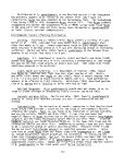 1971
1973
1975
\
\
Figure 31.
1971-1976
Distribution of Najjy^sp,, Maryland Chesapeake Bay,
101
image:
1971
1973
1975
\
\
Figure 31.
1971-1976
Distribution of Najjy^sp,, Maryland Chesapeake Bay,
101
image:
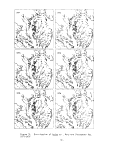 Since Najas spp. have been considered pest species in the past, they have
been used extensively in herbicide control experiments. Table 15 lists some
of the herbicides that are discussed in Chater 4 and their effects on Najas sp.
Productivity
Literature has little to reveal concerning the productivity of Najas sp.
Wetzel (1975) cited the work of Hough (1974) who studied photorespiration and
dark respiration. Hough found a 10-fold increase in respiration during the
fall compared to the summer.
Utilization
Martin and Uhler (1939) rated N. guadalupensis as excellent in food value
for waterfowl. Birds were found to eat both the seeds and the leafy plant
parts. Many species of Najas provide food for Tilapia melanopleura. an econo-
mically valuable fish species (Cook et al. 1974). Shuette and Alder (1929b_)
firmly stated that Najas spp. were of no economic importance. Several years
later, USDA (1939) recommended the use of N_. guadalupensis in the establishment
of permanent waterfowl impoundments.
N. guadalupensis appears to be high in crude protein and low in dry weight
yield (Mitchell 1974). Comparisons of crude protein content in Najas guadalupensis
and young alfalfa hay determined that Najas contained 22 percent dry weight as
protein compared to 19 percent for alfalfa. Najas would appear to be a potential
valuable protein source except for its low dry weight yield. Mitchell (1974)
lists Najas as yielding the lowest dry weight of 18 species of emergent, ter-
restrial and submerged plants. Typha latifolia ranked highest with 15.3 t/ha
dry weight while N_. guadalupensis yielded only 1.1 t/ha dry weight.
102
image:
Since Najas spp. have been considered pest species in the past, they have
been used extensively in herbicide control experiments. Table 15 lists some
of the herbicides that are discussed in Chater 4 and their effects on Najas sp.
Productivity
Literature has little to reveal concerning the productivity of Najas sp.
Wetzel (1975) cited the work of Hough (1974) who studied photorespiration and
dark respiration. Hough found a 10-fold increase in respiration during the
fall compared to the summer.
Utilization
Martin and Uhler (1939) rated N. guadalupensis as excellent in food value
for waterfowl. Birds were found to eat both the seeds and the leafy plant
parts. Many species of Najas provide food for Tilapia melanopleura. an econo-
mically valuable fish species (Cook et al. 1974). Shuette and Alder (1929b_)
firmly stated that Najas spp. were of no economic importance. Several years
later, USDA (1939) recommended the use of N_. guadalupensis in the establishment
of permanent waterfowl impoundments.
N. guadalupensis appears to be high in crude protein and low in dry weight
yield (Mitchell 1974). Comparisons of crude protein content in Najas guadalupensis
and young alfalfa hay determined that Najas contained 22 percent dry weight as
protein compared to 19 percent for alfalfa. Najas would appear to be a potential
valuable protein source except for its low dry weight yield. Mitchell (1974)
lists Najas as yielding the lowest dry weight of 18 species of emergent, ter-
restrial and submerged plants. Typha latifolia ranked highest with 15.3 t/ha
dry weight while N_. guadalupensis yielded only 1.1 t/ha dry weight.
102
image:
 Table 15. Herbicide control of Najas sp.
Herbicide
Diquat
1st year
+ paraquat 2nd year
Diquat
(4 week exposure)
Diquat
(16 weeks after exposure)
Paraquat
1st year
+ paraquat 2nd year
Paraquat
(16 weeks after exposure)
Paraquat
(4 week exposure)
Fenac
1st year
2nd year
Diquat
1st year
+ paraquat 2nd year
Simazine
1st year
2nd year
Diquat and Simazine
1st year
+ paraquat 2nd year
Endothal
Linuron
1st year
2nd year
Paraquat and Linuron
1st year
2nd year
Appl icati on
rate
2.75 kg/ha
1.1 kg/ha
1 ppm
5 ppm
10 ppm
1 ppm
2.75 kg/ha
1.1 kg/ha
1 ppm
1 ppm
5 ppm
10 ppm
11.0 kg/ha
none
0.66 kg/ha
11.0 kg/ha
11.0 kg/ha
none
0.66 kg/ha
11.0 kg/ha
1.1 kg/ha
1 ppm
5 ppm
10 ppm
11.0 kg/ha
none
0.1 kg/ha
5.5 kg/ha
none
Control
complete
complete
98%
100%
100%
85%
complete
complete
90%
87%
100%
100%
complete
complete
complete
complete
complete
complete
complete
complete
complete
99%
100%
100%
complete
complete
complete
complete
compl ete
Source
Lawrence 1965
Lawrence 1965
Blackburn 1963
Blackburn 1963
Blackburn and Wei don
Blackburn and Weldon
Lawrence 1965
Lawrence 1965
Blackburn and Weldon
Blackburn 1963
Blackburn 1963
Blackburn 1963
Lawrence 1965
Lawrence 1965
Lawrence 1965
Lawrence 1965
Lawrence 1965
Lawrence 1965
Lawrence 1965
Lawrence 1965
Lawrence 1965
Blackburn 1963
Blackburn 1963
Blackburn 1963
Lawrence 1965
Lawrence 1965
Lawrence 1965
Lawrence 1965
Lawrence 1965
1964
1964
1064
103
image:
Table 15. Herbicide control of Najas sp.
Herbicide
Diquat
1st year
+ paraquat 2nd year
Diquat
(4 week exposure)
Diquat
(16 weeks after exposure)
Paraquat
1st year
+ paraquat 2nd year
Paraquat
(16 weeks after exposure)
Paraquat
(4 week exposure)
Fenac
1st year
2nd year
Diquat
1st year
+ paraquat 2nd year
Simazine
1st year
2nd year
Diquat and Simazine
1st year
+ paraquat 2nd year
Endothal
Linuron
1st year
2nd year
Paraquat and Linuron
1st year
2nd year
Appl icati on
rate
2.75 kg/ha
1.1 kg/ha
1 ppm
5 ppm
10 ppm
1 ppm
2.75 kg/ha
1.1 kg/ha
1 ppm
1 ppm
5 ppm
10 ppm
11.0 kg/ha
none
0.66 kg/ha
11.0 kg/ha
11.0 kg/ha
none
0.66 kg/ha
11.0 kg/ha
1.1 kg/ha
1 ppm
5 ppm
10 ppm
11.0 kg/ha
none
0.1 kg/ha
5.5 kg/ha
none
Control
complete
complete
98%
100%
100%
85%
complete
complete
90%
87%
100%
100%
complete
complete
complete
complete
complete
complete
complete
complete
complete
99%
100%
100%
complete
complete
complete
complete
compl ete
Source
Lawrence 1965
Lawrence 1965
Blackburn 1963
Blackburn 1963
Blackburn and Wei don
Blackburn and Weldon
Lawrence 1965
Lawrence 1965
Blackburn and Weldon
Blackburn 1963
Blackburn 1963
Blackburn 1963
Lawrence 1965
Lawrence 1965
Lawrence 1965
Lawrence 1965
Lawrence 1965
Lawrence 1965
Lawrence 1965
Lawrence 1965
Lawrence 1965
Blackburn 1963
Blackburn 1963
Blackburn 1963
Lawrence 1965
Lawrence 1965
Lawrence 1965
Lawrence 1965
Lawrence 1965
1964
1964
1064
103
image:
 CHAPTER 2
THE ROLE OF SUBMERGED AQUATIC VEGETATION
INTRODUCTION
Submerged aquatic vegetation is an integral part of an estuarine system
such as the Chesapeake Bay. Submerged macrophytes constitute the principal
food source for waterfowl and some fish; they provide, direct or indirect,
food and shelter for many of the small host organisms that are eaten by fish
and other predators; the spawning activities of certain organisms require
them; they purify the water of such noxious substances as carbonic acid and
return oxygen; they shade the underlying waters and sediments from solar
heating; reduce turbidity by precipitating fine sediments; and provide an
important source of detritus. The assimilation of inorganic substances into
organic compounds usable by organisms enhances the importance of these plants
as a vital link in the food chain. Functioning as prime areas for hiding and
breeding, this vegetation group provides surfaces for attachment of eggs.
Also, an abundance of animal life, including insects, crustacean, molluscan,
fish and others find excellent feeding grounds on SAV (Baker 1916).
Submerged macrophytes help stabilize sediments and reduce shoreline
erosion. Bays with benthic flora have been shown to have relatively stable
metabolism with less fluctuation in comparison to plankton dominated bays
(Odum and Hoskin 1958). SAV further functions in the estuarine nutrient cycle
as a nutrient trap for dissolved phosphorus and nitrogen (Clark et al. 1973).
Though not presently utilized for such purposes in the Chesapeake Bay
area, aquatic plants serve as livestock food, human food, soil additives, fuel
and wastewater treatment in various other parts of the world. Primary
utilization in the Chesapeake Bay area is for wildlife conservation.
WATERFOWL
The Chesapeake Bay is an important waterfowl feeding area used by migrating
and wintering birds. Migration patterns can be classified according to
particular flyways and specific migration routes (Bellrose 1976). Distinguish-
ing a Flyway is a useful tool for interpreting waterfowl population trends
since migratory birds show greater affinity to a particular Flyway than to the
country as a whole. Flyways cover extensive areas and show population movement
from the general north-south direction. Migration routes, however, are more
clearly defined since they are 16 km wide at most and birds are directed to
river valleys, lakes and sea coasts that are in sight.
104
image:
CHAPTER 2
THE ROLE OF SUBMERGED AQUATIC VEGETATION
INTRODUCTION
Submerged aquatic vegetation is an integral part of an estuarine system
such as the Chesapeake Bay. Submerged macrophytes constitute the principal
food source for waterfowl and some fish; they provide, direct or indirect,
food and shelter for many of the small host organisms that are eaten by fish
and other predators; the spawning activities of certain organisms require
them; they purify the water of such noxious substances as carbonic acid and
return oxygen; they shade the underlying waters and sediments from solar
heating; reduce turbidity by precipitating fine sediments; and provide an
important source of detritus. The assimilation of inorganic substances into
organic compounds usable by organisms enhances the importance of these plants
as a vital link in the food chain. Functioning as prime areas for hiding and
breeding, this vegetation group provides surfaces for attachment of eggs.
Also, an abundance of animal life, including insects, crustacean, molluscan,
fish and others find excellent feeding grounds on SAV (Baker 1916).
Submerged macrophytes help stabilize sediments and reduce shoreline
erosion. Bays with benthic flora have been shown to have relatively stable
metabolism with less fluctuation in comparison to plankton dominated bays
(Odum and Hoskin 1958). SAV further functions in the estuarine nutrient cycle
as a nutrient trap for dissolved phosphorus and nitrogen (Clark et al. 1973).
Though not presently utilized for such purposes in the Chesapeake Bay
area, aquatic plants serve as livestock food, human food, soil additives, fuel
and wastewater treatment in various other parts of the world. Primary
utilization in the Chesapeake Bay area is for wildlife conservation.
WATERFOWL
The Chesapeake Bay is an important waterfowl feeding area used by migrating
and wintering birds. Migration patterns can be classified according to
particular flyways and specific migration routes (Bellrose 1976). Distinguish-
ing a Flyway is a useful tool for interpreting waterfowl population trends
since migratory birds show greater affinity to a particular Flyway than to the
country as a whole. Flyways cover extensive areas and show population movement
from the general north-south direction. Migration routes, however, are more
clearly defined since they are 16 km wide at most and birds are directed to
river valleys, lakes and sea coasts that are in sight.
104
image:
 The two most important migration paths pertinent to the Bay are the
eastern route, primarily through Quebec, and the route from the central and
northwest Canadian interior breeding grounds (Lincoln 1953; Bellrose 1976).
Some Greater Snow Geese and American Brant, originating as far north as the
eastern Artie islands and Greenland coast, partly follow coastal routes to Mid-
Atlantic bays and sounds. A more interior route directs Black Ducks and
Canada Geese from northern points of Quebec and Ontario.
Most diving ducks of the genus Aythya and a large portion of the dabbling
ducks are produced in the north central part of the continent and migrate
southward through the Great Lakes region (Bellrose 1976). Thus, a northwest
to southeast route is pursued by Canvasback, Redhead, and Greater and Lesser
Scaup wintering in Chesapeake Bay, Back Bay and other Mid-Atlantic coastal
waters.
For the purpose of this report, waterfowl species inhabiting the Bay area
are arranged into genera and represented by nomenclature used by Bellrose (1976)
(see Table 16).
A review of literature (Stewart and Manning 1958; Addy 1953; Longwell and
Stotts 1958; Stotts 1955; Henny and Holgersen 1974) indicates various waterfowl
species in Chesapeake Bay are undergoing changes in distribution, population
size and feeding habits. Data sources monitoring such changes include aerial
population counts and gullet and gizzard food content analyses. Observations
of banded birds are an additional information source used to trace harvest
patterns, mortality, migration corridors and breeding ground derivations.
Whistling Swan patterns also have been studied by using collar bands which
facilitate multiple resighting of birds. Radio telemetry is another tracing
method with a normal recovery range of 8 to 240 km (Sladen 1975). About 1,000
Canada Geese are banded each winter from primary Eastern Shore flocks to
monitor the status of the population (Stotts, personal communication).
Observations of production and band recoveries of diving ducks and also dabbling
ducks such as Gadwalls and Black Ducks have indicated changes in the breeding
range and migration routes for these species.
Population Trends of Wintering Waterfowl in Chesapeake Bay
Information on the distribution and population count for all waterfowl
species of the United States is available from the U.S. Bureau of Sport
Fisheries and Wildlife, Migratory Bird and Habitat Research Laboratory, Laurel,
Maryland. This annual aerial continental survey (January inventory), initiated
in 1948, is presently ongoing in cooperation with State and provincial con-
servation departments. Graphs of the population trends for eight species of
waterfowl inhabiting the Atlantic Flyway and the Chesapeake Bay region are
represented in Figure 32.
The two most abundant puddle ducks on Chesapeake Bay are Black Ducks and
Mallards. Generally, Black Ducks and Mallards have maintained fairly stable
populations after declines from outstanding highs observed in the mid-1950's.
The high population of Mallards was a result of excellent water conditions on
the western and northern breeding grounds succeeded by poor water conditions in
105
image:
The two most important migration paths pertinent to the Bay are the
eastern route, primarily through Quebec, and the route from the central and
northwest Canadian interior breeding grounds (Lincoln 1953; Bellrose 1976).
Some Greater Snow Geese and American Brant, originating as far north as the
eastern Artie islands and Greenland coast, partly follow coastal routes to Mid-
Atlantic bays and sounds. A more interior route directs Black Ducks and
Canada Geese from northern points of Quebec and Ontario.
Most diving ducks of the genus Aythya and a large portion of the dabbling
ducks are produced in the north central part of the continent and migrate
southward through the Great Lakes region (Bellrose 1976). Thus, a northwest
to southeast route is pursued by Canvasback, Redhead, and Greater and Lesser
Scaup wintering in Chesapeake Bay, Back Bay and other Mid-Atlantic coastal
waters.
For the purpose of this report, waterfowl species inhabiting the Bay area
are arranged into genera and represented by nomenclature used by Bellrose (1976)
(see Table 16).
A review of literature (Stewart and Manning 1958; Addy 1953; Longwell and
Stotts 1958; Stotts 1955; Henny and Holgersen 1974) indicates various waterfowl
species in Chesapeake Bay are undergoing changes in distribution, population
size and feeding habits. Data sources monitoring such changes include aerial
population counts and gullet and gizzard food content analyses. Observations
of banded birds are an additional information source used to trace harvest
patterns, mortality, migration corridors and breeding ground derivations.
Whistling Swan patterns also have been studied by using collar bands which
facilitate multiple resighting of birds. Radio telemetry is another tracing
method with a normal recovery range of 8 to 240 km (Sladen 1975). About 1,000
Canada Geese are banded each winter from primary Eastern Shore flocks to
monitor the status of the population (Stotts, personal communication).
Observations of production and band recoveries of diving ducks and also dabbling
ducks such as Gadwalls and Black Ducks have indicated changes in the breeding
range and migration routes for these species.
Population Trends of Wintering Waterfowl in Chesapeake Bay
Information on the distribution and population count for all waterfowl
species of the United States is available from the U.S. Bureau of Sport
Fisheries and Wildlife, Migratory Bird and Habitat Research Laboratory, Laurel,
Maryland. This annual aerial continental survey (January inventory), initiated
in 1948, is presently ongoing in cooperation with State and provincial con-
servation departments. Graphs of the population trends for eight species of
waterfowl inhabiting the Atlantic Flyway and the Chesapeake Bay region are
represented in Figure 32.
The two most abundant puddle ducks on Chesapeake Bay are Black Ducks and
Mallards. Generally, Black Ducks and Mallards have maintained fairly stable
populations after declines from outstanding highs observed in the mid-1950's.
The high population of Mallards was a result of excellent water conditions on
the western and northern breeding grounds succeeded by poor water conditions in
105
image:
 Table 16. Waterfowl of the Chesapeake Bay3
Family Anatidae (Swans, Geese and Ducks)
Subfamily Anserinae (Swans, Geese)
Cygnus columbianus (Whistling Swan)
Cygnus olor (Mut¥~Swan)...recently introduced
Cygnus buccinator (Trumpeter Swan)... formerly present
Anser c. caerulescens (Lesser Snow Goose)
Anser caerulescens atlantica (Greater Snow Goose)
Brantja canadensis (Canada Goose)
Branta bernicla hrota (Atlantic Brant)
Subfamily Anatinae (Surface-Feeding and Diving Ducks, Mergansers,
Stiff-Tailed Ducks)
Aix sponsa (Wood Duck)
Anas penelope (European Wigeon)... rare
Anas americana (American Wigeon)
Anas strepera (Gadwal1)
Anas crecca carolinensis (Green-winged Teal)
Anas platyrhynchos platyrhynchos (Mallard)
Anas rubripes (Black Duck)
Anas acuta acuta (Pintail)
Anas discors (Blue-winged Teal)
Anas clypeata (Northern Shoveler)
Aythya valisineria (Canvasback)
Aythya amer i cana~TRedhead)
Aythya collaris (Ring-necked Duck)
Aythya man'la mariloides (Greater Scaup)
Aythya affinis (Lesser Scaup)
Clangula hyemalis (Oldsquaw)
Melanitta nigra americana (Black Scoter)
Melanitta perspicillata (Surf Scoter)
Melanitta fusca deglandi (White-winged Scoter)
Bucephala albeola (Bufflehead)
Bucephala clangula americana (Common Goldeneye)
Mergus cucullatus (Hooded Merganser)
Mergus ¥errator~TReh-breasted Merganser)
Mergus merganser americanus (Common Merganser)
Oxyura jamaicensis ribida (Ruddy Duck)
a Bell rose 1976
106
image:
Table 16. Waterfowl of the Chesapeake Bay3
Family Anatidae (Swans, Geese and Ducks)
Subfamily Anserinae (Swans, Geese)
Cygnus columbianus (Whistling Swan)
Cygnus olor (Mut¥~Swan)...recently introduced
Cygnus buccinator (Trumpeter Swan)... formerly present
Anser c. caerulescens (Lesser Snow Goose)
Anser caerulescens atlantica (Greater Snow Goose)
Brantja canadensis (Canada Goose)
Branta bernicla hrota (Atlantic Brant)
Subfamily Anatinae (Surface-Feeding and Diving Ducks, Mergansers,
Stiff-Tailed Ducks)
Aix sponsa (Wood Duck)
Anas penelope (European Wigeon)... rare
Anas americana (American Wigeon)
Anas strepera (Gadwal1)
Anas crecca carolinensis (Green-winged Teal)
Anas platyrhynchos platyrhynchos (Mallard)
Anas rubripes (Black Duck)
Anas acuta acuta (Pintail)
Anas discors (Blue-winged Teal)
Anas clypeata (Northern Shoveler)
Aythya valisineria (Canvasback)
Aythya amer i cana~TRedhead)
Aythya collaris (Ring-necked Duck)
Aythya man'la mariloides (Greater Scaup)
Aythya affinis (Lesser Scaup)
Clangula hyemalis (Oldsquaw)
Melanitta nigra americana (Black Scoter)
Melanitta perspicillata (Surf Scoter)
Melanitta fusca deglandi (White-winged Scoter)
Bucephala albeola (Bufflehead)
Bucephala clangula americana (Common Goldeneye)
Mergus cucullatus (Hooded Merganser)
Mergus ¥errator~TReh-breasted Merganser)
Mergus merganser americanus (Common Merganser)
Oxyura jamaicensis ribida (Ruddy Duck)
a Bell rose 1976
106
image:
 r-~ 10 LO •=!• oo CM
(OOO'OOIX) spjiq ±o
LO
10
o
10
LO
LO
to
-a
t/> s-
s- ra
03 r—
cu •—
>- (O
CO
o
/
L LO
to
in o.
S- 3
(C n3
O) O
LO >- 00
OsJ
00
C\J
(OOO'OOIX) spuiq
LO
LO
to
O)
•I—
o
d)
Q.
to
cu
-M
ns
ns
CQ
OJ
(J (O
(O (/)
r— O»
•M ^:
=t o
II II
U_ CQ
«C O
LO
<• m CM
(OOO'OOIX) spuiq ^c
LO
to Q
ra -^
CU O
LO >~ *°
10 S
LO
LO
LO O LO O S O LO
CO CO CM CM t—I •—I O
(OOO'OOLX) spuiq ^
u
to ns
S- .0
ra l^
O) ra
>->
LO
LO
a.
to
cu
o
<a
S-
OJ
>
(U
to
c/)
-a
ra
a.
o
Q.
C\J
OO
0)
CD
107
image:
r-~ 10 LO •=!• oo CM
(OOO'OOIX) spjiq ±o
LO
10
o
10
LO
LO
to
-a
t/> s-
s- ra
03 r—
cu •—
>- (O
CO
o
/
L LO
to
in o.
S- 3
(C n3
O) O
LO >- 00
OsJ
00
C\J
(OOO'OOIX) spuiq
LO
LO
to
O)
•I—
o
d)
Q.
to
cu
-M
ns
ns
CQ
OJ
(J (O
(O (/)
r— O»
•M ^:
=t o
II II
U_ CQ
«C O
LO
<• m CM
(OOO'OOIX) spuiq ^c
LO
to Q
ra -^
CU O
LO >~ *°
10 S
LO
LO
LO O LO O S O LO
CO CO CM CM t—I •—I O
(OOO'OOLX) spuiq ^
u
to ns
S- .0
ra l^
O) ra
>->
LO
LO
a.
to
cu
o
<a
S-
OJ
>
(U
to
c/)
-a
ra
a.
o
Q.
C\J
OO
0)
CD
107
image:
 I— <1> LO ^" CO CM i—
O , O O p CD O O
(OOO'OOIX) spuiq ic
LT>
o
r-
LO
to
-a
<o
CD
</) .C
S- O)
re i—
OMM-
>- V
3
CQ
LO
LO
...•i^—'
*f CM O CO l£)
LO
in
c.
oo
CJ)
LO
vo
i-
fO i
CD
>-
^- CM
LO
LO
(OOO'OOTX) spaiq ^
3 re
>>CQ
U_ d)
_^:
o re
•i- OJ
-i-> Q.
c re
re to
i— OJ
•M ^=
•a: o
ii n
U- CQ
ca; <_>
LO
CO
Lf>
CM
co
LO
CD
CD
to CD
S_
re re
cu ~o
LO
LO
n CM CM
(OOO'OOTX)
(OOO'OOIX) sp-uq
-a
§
c
+J
c
o
CM
ro
2:
3
CD
108
image:
I— <1> LO ^" CO CM i—
O , O O p CD O O
(OOO'OOIX) spuiq ic
LT>
o
r-
LO
to
-a
<o
CD
</) .C
S- O)
re i—
OMM-
>- V
3
CQ
LO
LO
...•i^—'
*f CM O CO l£)
LO
in
c.
oo
CJ)
LO
vo
i-
fO i
CD
>-
^- CM
LO
LO
(OOO'OOTX) spaiq ^
3 re
>>CQ
U_ d)
_^:
o re
•i- OJ
-i-> Q.
c re
re to
i— OJ
•M ^=
•a: o
ii n
U- CQ
ca; <_>
LO
CO
Lf>
CM
co
LO
CD
CD
to CD
S_
re re
cu ~o
LO
LO
n CM CM
(OOO'OOTX)
(OOO'OOIX) sp-uq
-a
§
c
+J
c
o
CM
ro
2:
3
CD
108
image:
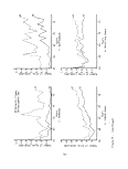 the late 1950s (Perry 1977). Data for individual puddle duck species show
that population trends for the Atlantic Flyway parallel those of Chesapeake Bay
(see Graphs A and B) though Mallards have undergone greater population fluxes
in the Atlantic Flyway than the Chesapeake Bay.
Total populations for members of the diving ducks of genus Aythya showed
trends similar to the puddle ducks (refer to Figure 32, C, D, E and F). The
Canvasback populations of Chesapeake Bay in early survey years comprised nearly
50 percent of the Flyway population. The average total population size of
Canvasbacks was higher in the 1960s when vegetation was more readily available
in Chesapeake Bay. Canvasbacks have adapted to available invertebrates as
their food resources owing to vegetation reductions.
Scaups, which are the second most important diving duck species in the Bay,
remained relatively stable during the past 30 years in the Chesapeake Bay.
The Bay populations of Redheads has been on the decline; Atlantic Flyway
numbers increased erratically with a high in 1966 which was not reflected in the
Chesapeake Bay population. This species shows the greatest dependence on SAV
of all the diving ducks. In both the Atlantic Flyway and Chesapeake Bay, the
population of the Buffieheads, a traditional animal feeder (McAtee 1911), has
fluctuated upward.
The Canada Goose population has been rising steadily over the past 20 years
(see Figure 32, Graph G). Field feeding on corn (Zea mays) has enlarged the
range and carrying capacity for this species. Similarly, Whistling Swans have
changed their feeding habits from submerged aquatic vegetation to field feeding
(see Figure 32 Graph H). In the past decades, the population count of Whistling
Swans has decreased slightly in the Bay and increased on the Atlantic Flyway.
The Mute Swan was recently introduced into the Eastern Shore of the
Chesapeake Bay when five birds escaped from captivity in 1962. By 1970 there
were approximately 27 birds inhabiting the Miles River area. Since 1970, the
Mute Swan population has increased yearly by almost 40 percent (Fenwick personal
communication). If this rate of increase continues, there could be about 10,000
mutes in the Bay by 1988. Bay area researchers are concerned that the Mute Swan
may be causing interspecific competition for vegetable food resources of
native waterfowl. A single Mute Swan can consume up to about 4.6 kg of SAV
daily (Fenwick, personal communication).
Feeding Habits of Predominant Waterfowl of The Chesapeake Bay
Changes in the availability of traditional food sources is regarded by Bay
area researchers as a primary cause of Chesapeake Bay waterfowl population
fluctuations (Rawls, in press; Fenwick, personal communication; Stotts,
personal communication; Perry et al. 1976). Not only have there been
fluctuations in submerged aquatic vegetation abundance but also in the avail-
ability of the brackish water clam (Rangia cuneata).
In order to study past and present feeding habits, ducks can be conveniently
divided into two groups based on physical morphology. Diving ducks exhibit a
posterior leg position which makes terrestrial movement difficult and restricts
feeding to an aquatic environment. Dabbling ducks have a more forward leg
109
image:
the late 1950s (Perry 1977). Data for individual puddle duck species show
that population trends for the Atlantic Flyway parallel those of Chesapeake Bay
(see Graphs A and B) though Mallards have undergone greater population fluxes
in the Atlantic Flyway than the Chesapeake Bay.
Total populations for members of the diving ducks of genus Aythya showed
trends similar to the puddle ducks (refer to Figure 32, C, D, E and F). The
Canvasback populations of Chesapeake Bay in early survey years comprised nearly
50 percent of the Flyway population. The average total population size of
Canvasbacks was higher in the 1960s when vegetation was more readily available
in Chesapeake Bay. Canvasbacks have adapted to available invertebrates as
their food resources owing to vegetation reductions.
Scaups, which are the second most important diving duck species in the Bay,
remained relatively stable during the past 30 years in the Chesapeake Bay.
The Bay populations of Redheads has been on the decline; Atlantic Flyway
numbers increased erratically with a high in 1966 which was not reflected in the
Chesapeake Bay population. This species shows the greatest dependence on SAV
of all the diving ducks. In both the Atlantic Flyway and Chesapeake Bay, the
population of the Buffieheads, a traditional animal feeder (McAtee 1911), has
fluctuated upward.
The Canada Goose population has been rising steadily over the past 20 years
(see Figure 32, Graph G). Field feeding on corn (Zea mays) has enlarged the
range and carrying capacity for this species. Similarly, Whistling Swans have
changed their feeding habits from submerged aquatic vegetation to field feeding
(see Figure 32 Graph H). In the past decades, the population count of Whistling
Swans has decreased slightly in the Bay and increased on the Atlantic Flyway.
The Mute Swan was recently introduced into the Eastern Shore of the
Chesapeake Bay when five birds escaped from captivity in 1962. By 1970 there
were approximately 27 birds inhabiting the Miles River area. Since 1970, the
Mute Swan population has increased yearly by almost 40 percent (Fenwick personal
communication). If this rate of increase continues, there could be about 10,000
mutes in the Bay by 1988. Bay area researchers are concerned that the Mute Swan
may be causing interspecific competition for vegetable food resources of
native waterfowl. A single Mute Swan can consume up to about 4.6 kg of SAV
daily (Fenwick, personal communication).
Feeding Habits of Predominant Waterfowl of The Chesapeake Bay
Changes in the availability of traditional food sources is regarded by Bay
area researchers as a primary cause of Chesapeake Bay waterfowl population
fluctuations (Rawls, in press; Fenwick, personal communication; Stotts,
personal communication; Perry et al. 1976). Not only have there been
fluctuations in submerged aquatic vegetation abundance but also in the avail-
ability of the brackish water clam (Rangia cuneata).
In order to study past and present feeding habits, ducks can be conveniently
divided into two groups based on physical morphology. Diving ducks exhibit a
posterior leg position which makes terrestrial movement difficult and restricts
feeding to an aquatic environment. Dabbling ducks have a more forward leg
109
image:
 position which facilitates maneuverability on land but does not restrict aquatic
movement. Table 17 lists in detail the feeding habits of the major waterfowl in
the Chesapeake Bay. The following section discusses these feeding habits and the
changes that have been noted.
Canvasbacks, one of the diving ducks, have fluctuated in number over the past
few decades. Traditionally, wintering Canvasbacks were vegetation feeders, their
mainstays being wild celery and sago pondweed. In the 1950s it was found that
"Cans" existed on a mixed diet of vegetation and invertebrates (Stewart 1962).
Recent declines of submerged aquatic vegetation has had an effect on the number
of not only Canvasbacks but of most waterfowl wintering in the various regions of
the Bay (Perry et al. 1976).
Canvasbacks have adapted their diet to abundances of particular foods. This
flexibility has enabled the "Cans" to adapt to a situation of decreased submerged
vegetation and become independent of vegetable foods. Currently their diet con-
sists of about 48 percent animal and 52 percent vegetable matter (Rawls in press).
Baltic and soft shelled clams constitute the main animal foods while corn and red-
head grass are the primary vegetable foods. The availability of animals, particu-
larly the brackish water clam may have caused yearly fluctuations in the Canyasback
populations on the Western Shore. In 1968, only 11 percent of Canvasbacks wintered
there; while in 1971 the population on the Western Shore increased to 87 percent.
The availablity of Rangia to Canvasbacks has decreased due to diminished spawning
and excessive clam size (Perry et al. 1976).
The Redhead, another diving duck, presently shows a greater dependence on
vegetation than does the Canvasback. Gizzard studies by Rawls (in press) showed
that the Redhead's diet consisted of about 76 percent vegetable and about 23 percent
animal foods. Studies by Stewart (1962) showed that leaves, stems, root stalks
and seeds of various species of rooted aquatics were the predominant foods.
The Lesser Scaup, also a diving duck, feeds on both vegetable and animal foods.
Stewart (1962) showed that various species of mollusk were the principal food
sources. Rawls (in press) determined animal foods comprised almost 48 percent of
their diets. Percent vegetable intake over the 1959 to 1968 study constituted
slightly over 52 percent.
Two other diving ducks, the Bufflehead and Goldeneye, are traditionally
mollusk and crustacean feeders but will also consume vegetable matter (Stewart
1962). Rawls (in press) found that in the Chesapeake Bay, over 67 percent of the
Buffleheads total food intake was animal. A 1962 study done in Back Bay and
Currituck Sound showed that Bufflehead's subsisted on the seeds of widgeongrass
and naiad, with plants comprising 64 percent of their diet (Sincock 1962). Recent
work in Chesapeake Bay by Rawls (in press) showed that the Goldeneye has an animal
diet similar to the Bufflehead: 63 percent animal food and 37 percent vegetable food,
Dabbling ducks such as Mallards and Black Ducks are able to feed in both
aquatic and terrestrial environments. Mallards have been found to eat almost
anything available (Bellrose 1976) but subsist almost entirely on a vegetable diet
in the Chesapeake Bay (Stewart 1962; Rawls in press). The natural foods of
Mallards differ sharply in freshwater estuarine marshes compared to brackish
110
image:
position which facilitates maneuverability on land but does not restrict aquatic
movement. Table 17 lists in detail the feeding habits of the major waterfowl in
the Chesapeake Bay. The following section discusses these feeding habits and the
changes that have been noted.
Canvasbacks, one of the diving ducks, have fluctuated in number over the past
few decades. Traditionally, wintering Canvasbacks were vegetation feeders, their
mainstays being wild celery and sago pondweed. In the 1950s it was found that
"Cans" existed on a mixed diet of vegetation and invertebrates (Stewart 1962).
Recent declines of submerged aquatic vegetation has had an effect on the number
of not only Canvasbacks but of most waterfowl wintering in the various regions of
the Bay (Perry et al. 1976).
Canvasbacks have adapted their diet to abundances of particular foods. This
flexibility has enabled the "Cans" to adapt to a situation of decreased submerged
vegetation and become independent of vegetable foods. Currently their diet con-
sists of about 48 percent animal and 52 percent vegetable matter (Rawls in press).
Baltic and soft shelled clams constitute the main animal foods while corn and red-
head grass are the primary vegetable foods. The availability of animals, particu-
larly the brackish water clam may have caused yearly fluctuations in the Canyasback
populations on the Western Shore. In 1968, only 11 percent of Canvasbacks wintered
there; while in 1971 the population on the Western Shore increased to 87 percent.
The availablity of Rangia to Canvasbacks has decreased due to diminished spawning
and excessive clam size (Perry et al. 1976).
The Redhead, another diving duck, presently shows a greater dependence on
vegetation than does the Canvasback. Gizzard studies by Rawls (in press) showed
that the Redhead's diet consisted of about 76 percent vegetable and about 23 percent
animal foods. Studies by Stewart (1962) showed that leaves, stems, root stalks
and seeds of various species of rooted aquatics were the predominant foods.
The Lesser Scaup, also a diving duck, feeds on both vegetable and animal foods.
Stewart (1962) showed that various species of mollusk were the principal food
sources. Rawls (in press) determined animal foods comprised almost 48 percent of
their diets. Percent vegetable intake over the 1959 to 1968 study constituted
slightly over 52 percent.
Two other diving ducks, the Bufflehead and Goldeneye, are traditionally
mollusk and crustacean feeders but will also consume vegetable matter (Stewart
1962). Rawls (in press) found that in the Chesapeake Bay, over 67 percent of the
Buffleheads total food intake was animal. A 1962 study done in Back Bay and
Currituck Sound showed that Bufflehead's subsisted on the seeds of widgeongrass
and naiad, with plants comprising 64 percent of their diet (Sincock 1962). Recent
work in Chesapeake Bay by Rawls (in press) showed that the Goldeneye has an animal
diet similar to the Bufflehead: 63 percent animal food and 37 percent vegetable food,
Dabbling ducks such as Mallards and Black Ducks are able to feed in both
aquatic and terrestrial environments. Mallards have been found to eat almost
anything available (Bellrose 1976) but subsist almost entirely on a vegetable diet
in the Chesapeake Bay (Stewart 1962; Rawls in press). The natural foods of
Mallards differ sharply in freshwater estuarine marshes compared to brackish
110
image:
 Table 17. Food habits of waterfowl in the upper Chesapeake Bay, Maryland9'5
Waterfowl
species
Canvasback
Redhead
Lesser Scaup
Bufflehead
Go! den eye
Mallard
Black Duck
Canada Goose
Animal Vegetable Total
food food %
% %
47.76 51.85 99.61 19.65
18.42
16.32
14.29
7.44
23.40 76.59 99.99 29.29
15.19
14.74
10.53
6.73
47.56 52.47 100.03 20.48
12.32
11.59
10.85
6.89
67.42 32.59 100.01 13.52
11.85
10.00
8.52
7.22
63.09 36.87 99.96 19.44
17.67
14.88
9.22
9.00
5.00 94.80 99.80 24.14
10.41
8.17
9.13
1.64
1.31
6.44 93.54 99.98 17.52
15.50
14.20
8.40
1.91
1.76
0.00 100.00 100.00 32.42
29.61
6.97
5.11
2.99
Predominant foods
% total volume
Baltic clam
Corn
Soft-shelled clam
Redhead grass
Widgeongrass
Corn
Redhead grass
Widgeongrass
Soft-shelled, Baltic and Mitchell's clams
Conrad's false mussel
Widgeongrass
Soft-shelled clam
Corn
Redhead grass
Mussel
Widgeongrass
Redhead grass
Barnacle
Fish
Mud crabs
Mud crab
Corn
Soft-shelled clam
Barnacle
Bivalves (unidentified fragments)
Corn
Redhead grass
Widgeongrass
Other submerged macrophytes
Conrad's false mussel
Soft-shelled clam
Corn
Redhead grass
Widgeongrass
Milfoil
Conrad's false mussel
Amphipods
Grasses (Gramineae)
Corn
Milfoil
White clover
Crab grass
aBased on waterfowl gizzards collected during 1959-1968 hunting seasons
^Rawls (in press)
111
image:
Table 17. Food habits of waterfowl in the upper Chesapeake Bay, Maryland9'5
Waterfowl
species
Canvasback
Redhead
Lesser Scaup
Bufflehead
Go! den eye
Mallard
Black Duck
Canada Goose
Animal Vegetable Total
food food %
% %
47.76 51.85 99.61 19.65
18.42
16.32
14.29
7.44
23.40 76.59 99.99 29.29
15.19
14.74
10.53
6.73
47.56 52.47 100.03 20.48
12.32
11.59
10.85
6.89
67.42 32.59 100.01 13.52
11.85
10.00
8.52
7.22
63.09 36.87 99.96 19.44
17.67
14.88
9.22
9.00
5.00 94.80 99.80 24.14
10.41
8.17
9.13
1.64
1.31
6.44 93.54 99.98 17.52
15.50
14.20
8.40
1.91
1.76
0.00 100.00 100.00 32.42
29.61
6.97
5.11
2.99
Predominant foods
% total volume
Baltic clam
Corn
Soft-shelled clam
Redhead grass
Widgeongrass
Corn
Redhead grass
Widgeongrass
Soft-shelled, Baltic and Mitchell's clams
Conrad's false mussel
Widgeongrass
Soft-shelled clam
Corn
Redhead grass
Mussel
Widgeongrass
Redhead grass
Barnacle
Fish
Mud crabs
Mud crab
Corn
Soft-shelled clam
Barnacle
Bivalves (unidentified fragments)
Corn
Redhead grass
Widgeongrass
Other submerged macrophytes
Conrad's false mussel
Soft-shelled clam
Corn
Redhead grass
Widgeongrass
Milfoil
Conrad's false mussel
Amphipods
Grasses (Gramineae)
Corn
Milfoil
White clover
Crab grass
aBased on waterfowl gizzards collected during 1959-1968 hunting seasons
^Rawls (in press)
111
image:
 water marshes within the Chesapeake Bay estuary. Stewart (1962) found that seeds
of smartweeds, soft stem and three-square bulrushes and bur reeds predominated
in freshwater, while in brackish water marshes, seeds of widgeongrass, pondweeds,
smartweeds and the leaves and stems of submerged aquatics were more important
food sources.
Black Ducks display feeding habits similar to Mallards with a diet consisting
mainly of plant food (Stewart 1962; Rawls in press). One notable difference be-
tween Mallards and Black Ducks was a higher consumption of sea lettuce by Black
Ducks (Rawls in press). Presently underway is a study by George Fenwick (The
Johns Hopkins University) of about 300 duck gizzards collected in Eastern Bay,
Miles River and Wye River from 1972 to 1976. Predominant species included in
the analysis are Black Duck, Wigeon, Mai lard,Scaup, Goldeneye, Bufflehead,
Old Squaw and Ruddy Duck. Though the study has not as yet been completed, a
tentative conclusion shows that submerged aquatic vegetation has been declining
as a waterfowl food source (Fenwick, personal communication). Fenwick further
hopes to show the impacts of the increased Mute Swan population on food avail-
ability to not only Whistling Swans but native diving and dabbling ducks.
Canada Geese are herbivores and have benefited from agricultural products
more than any other waterfowl species of North America (Bellrose 1976). The
population of this species has increased rapidly over the past three decades. It
has been estimated that with modern crop harvesting methods, 10 percent of the
crop remains after harvesting. Canada Geese have reduced their intake of
aquatic plants and turned to croplands along the Atlantic Flyway.
Whistling Swans have a diet that is similar to Canada Geese. These swans
now commonly feed on field grains and can cause crop damage (Sladen 1975).
Early observations of Whistling Swans (Bent 1925) suggested that their diet was
predominantly vegetable but they fed on some shellfish. Stomach analyses by
Martin et al. (1951) indicated a diet of emergent and submerged vegetation with
sago pondweed most common. Stewart and Manning (1958) found that Whistling Swans
in brackish estuary waters consumed widgeongrass (50 percent ) and mollusks
(40 percent), in addition to small quantities of redhead grass and sago pondweed.
In contrast, swans observed feeding in the fresh waters of the northern Chesapeake
Bay fed entirely on wild celery.
The Role of Myriophyllum spicatum as a Waterfowl Food Source
The extravagant growth of milfoil that infested the Chesapeake Bay in the
1960s caused some concern among waterfowl enthusiasts as to milfoil's use as
a waterfowl food source.
Based on information available at the time, Martin and Uhler (1939) had
determined that milfoil was a less than satisfactory food for ducks. Florschutz
(1969) analyzed the digestive tracts of three geese and 74 ducks from Back Bay
and Currituck Sound and found milfoil in all of the geese. Wigeons had ingested
large quantities of milfoil though Mallard and Black Duck digestive tracts showed
little milfoil. The average food content for all 77 waterfowl showed that 45.5
percent was Eurasian water-milfoil. Gadwalls contained the highest (88.9 percent)
by volume. Canada Geese followed with 83.0 percent which was higher than
112
image:
water marshes within the Chesapeake Bay estuary. Stewart (1962) found that seeds
of smartweeds, soft stem and three-square bulrushes and bur reeds predominated
in freshwater, while in brackish water marshes, seeds of widgeongrass, pondweeds,
smartweeds and the leaves and stems of submerged aquatics were more important
food sources.
Black Ducks display feeding habits similar to Mallards with a diet consisting
mainly of plant food (Stewart 1962; Rawls in press). One notable difference be-
tween Mallards and Black Ducks was a higher consumption of sea lettuce by Black
Ducks (Rawls in press). Presently underway is a study by George Fenwick (The
Johns Hopkins University) of about 300 duck gizzards collected in Eastern Bay,
Miles River and Wye River from 1972 to 1976. Predominant species included in
the analysis are Black Duck, Wigeon, Mai lard,Scaup, Goldeneye, Bufflehead,
Old Squaw and Ruddy Duck. Though the study has not as yet been completed, a
tentative conclusion shows that submerged aquatic vegetation has been declining
as a waterfowl food source (Fenwick, personal communication). Fenwick further
hopes to show the impacts of the increased Mute Swan population on food avail-
ability to not only Whistling Swans but native diving and dabbling ducks.
Canada Geese are herbivores and have benefited from agricultural products
more than any other waterfowl species of North America (Bellrose 1976). The
population of this species has increased rapidly over the past three decades. It
has been estimated that with modern crop harvesting methods, 10 percent of the
crop remains after harvesting. Canada Geese have reduced their intake of
aquatic plants and turned to croplands along the Atlantic Flyway.
Whistling Swans have a diet that is similar to Canada Geese. These swans
now commonly feed on field grains and can cause crop damage (Sladen 1975).
Early observations of Whistling Swans (Bent 1925) suggested that their diet was
predominantly vegetable but they fed on some shellfish. Stomach analyses by
Martin et al. (1951) indicated a diet of emergent and submerged vegetation with
sago pondweed most common. Stewart and Manning (1958) found that Whistling Swans
in brackish estuary waters consumed widgeongrass (50 percent ) and mollusks
(40 percent), in addition to small quantities of redhead grass and sago pondweed.
In contrast, swans observed feeding in the fresh waters of the northern Chesapeake
Bay fed entirely on wild celery.
The Role of Myriophyllum spicatum as a Waterfowl Food Source
The extravagant growth of milfoil that infested the Chesapeake Bay in the
1960s caused some concern among waterfowl enthusiasts as to milfoil's use as
a waterfowl food source.
Based on information available at the time, Martin and Uhler (1939) had
determined that milfoil was a less than satisfactory food for ducks. Florschutz
(1969) analyzed the digestive tracts of three geese and 74 ducks from Back Bay
and Currituck Sound and found milfoil in all of the geese. Wigeons had ingested
large quantities of milfoil though Mallard and Black Duck digestive tracts showed
little milfoil. The average food content for all 77 waterfowl showed that 45.5
percent was Eurasian water-milfoil. Gadwalls contained the highest (88.9 percent)
by volume. Canada Geese followed with 83.0 percent which was higher than
112
image:
 American Wigeons (71.0 percent). Mallards and Black Ducks were lowest with
11.0 percent and 14.3 percent, respectively.
Florschutz (1969) indicated that although the availability of higher
quality waterfowl food was reduced by the milfoil invasion, various waterfowl
species used milfoil as a food source. Subsequently, the waterfowl populations
of the inland waters of Virginia and North Carolina increased when total
Atlantic Flyway populations decreased. Florschutz concluded that these popula-
tion trends showed that milfoil was "not totally unacceptable" as a food
resource.
Contrary to waterfowl trends of Back Bay and Currituck Sound in the 1960s,
populations on the Susquehanna Flats showed marked declines. During this time,
milfoil displaced more than a dozen native rooted aquatic species (Bayley et al.
in press). January populations of waterfowl on the Flats averaged 4,900 during
early infestation of milfoil (1958-1961). During the milfoil peak, January
waterfowl counts on the Flats averaged only 390 birds. By 1965, when Vallisneria
returned to about 50 percent the level sustained prior to milfoil invasion, an
average of 4,860 birds wintered on the Flats.
Conclusions
An overall decline of Redheads and Whistling Swans suggests that the
diminishing supply of a traditional food source of submerged macrophytes is a
contributing factor. The Bufflehead, an animal feeder, has increased its
population size in the Chesapeake Bay during the past few decades. Canada
Geese, Mallards and Black Ducks have adapted to terrestrial feeding. Diving
ducks such as Canvasbacks, have adapted to a more animal diet. Apparently, a
decrease of a traditionally desired food source such as SAV results in several
options for native and migratory waterfowl. They can either seek an alternative
food source or compete for the diminishing food source. Either alternative
could result in population reductions and locale changes.
AQUATIC FAUNAL ASSOCIATIONS
Submerged aquatic vegetation functions as an essential link in the aquatic
faunal environment. SAV serves as both a direct and indirect food source; beds
provide breeding and protection areas; and a variety of organisms use SAV roots,
stems and leaves for attachment.
As a direct food source, SAV plant material, in both living and decaying
forms, provides food for a variety of vertebrates and invertebrates. Physa eats
the tender green shoots of Chara and Elodea; Planorbis lives entirely on sub-
merged aquatic plants; Ancylus consumes decaying plant material; and Ruppia
martima and Vailisneria spiralis can comprise up to 45 percent of the diet
of the sheepshead (Archosargus probatocephalus). SAV, as an important source of
detritus further serves as a food source for a wide variety of filter feeders.
By serving as habitat breeding and protection areas, SAV beds provide an
indirect food source for many species of fauna. Plant roots, stems and leaves
provide firm bases for attachment of such sedentary epibenthos as mussels,
barnacles and mollusks (Green 1968). Fish, such as the cownose ray (Rhinoptera
bonasusyactively feed on mollusks that inhabit SAV beds (Orth 1975a_). Marsh
113
image:
American Wigeons (71.0 percent). Mallards and Black Ducks were lowest with
11.0 percent and 14.3 percent, respectively.
Florschutz (1969) indicated that although the availability of higher
quality waterfowl food was reduced by the milfoil invasion, various waterfowl
species used milfoil as a food source. Subsequently, the waterfowl populations
of the inland waters of Virginia and North Carolina increased when total
Atlantic Flyway populations decreased. Florschutz concluded that these popula-
tion trends showed that milfoil was "not totally unacceptable" as a food
resource.
Contrary to waterfowl trends of Back Bay and Currituck Sound in the 1960s,
populations on the Susquehanna Flats showed marked declines. During this time,
milfoil displaced more than a dozen native rooted aquatic species (Bayley et al.
in press). January populations of waterfowl on the Flats averaged 4,900 during
early infestation of milfoil (1958-1961). During the milfoil peak, January
waterfowl counts on the Flats averaged only 390 birds. By 1965, when Vallisneria
returned to about 50 percent the level sustained prior to milfoil invasion, an
average of 4,860 birds wintered on the Flats.
Conclusions
An overall decline of Redheads and Whistling Swans suggests that the
diminishing supply of a traditional food source of submerged macrophytes is a
contributing factor. The Bufflehead, an animal feeder, has increased its
population size in the Chesapeake Bay during the past few decades. Canada
Geese, Mallards and Black Ducks have adapted to terrestrial feeding. Diving
ducks such as Canvasbacks, have adapted to a more animal diet. Apparently, a
decrease of a traditionally desired food source such as SAV results in several
options for native and migratory waterfowl. They can either seek an alternative
food source or compete for the diminishing food source. Either alternative
could result in population reductions and locale changes.
AQUATIC FAUNAL ASSOCIATIONS
Submerged aquatic vegetation functions as an essential link in the aquatic
faunal environment. SAV serves as both a direct and indirect food source; beds
provide breeding and protection areas; and a variety of organisms use SAV roots,
stems and leaves for attachment.
As a direct food source, SAV plant material, in both living and decaying
forms, provides food for a variety of vertebrates and invertebrates. Physa eats
the tender green shoots of Chara and Elodea; Planorbis lives entirely on sub-
merged aquatic plants; Ancylus consumes decaying plant material; and Ruppia
martima and Vailisneria spiralis can comprise up to 45 percent of the diet
of the sheepshead (Archosargus probatocephalus). SAV, as an important source of
detritus further serves as a food source for a wide variety of filter feeders.
By serving as habitat breeding and protection areas, SAV beds provide an
indirect food source for many species of fauna. Plant roots, stems and leaves
provide firm bases for attachment of such sedentary epibenthos as mussels,
barnacles and mollusks (Green 1968). Fish, such as the cownose ray (Rhinoptera
bonasusyactively feed on mollusks that inhabit SAV beds (Orth 1975a_). Marsh
113
image:
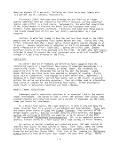 (1973) observed the predation by numerous fish on the epifauna of the
aquatic plants. Mi nidi a mi nidi a (common silversides), Apeltes quadracus
(four-spined stickleback) and Syngnathus fuscus (pipefish) were the
most abundant fish observed.
Baker (1918) found associations of Potamogeton perfoliatus,
Vanisneria spiral is, El odea canadensis, Ceratophyl 1 urn demersum,
Myripphyllum spicatum and Chara spp. with the mollusks Acel1 a haldemani
living on the leaves and stems and in the vegetation. By th in ia
tentaculata, Galba cataseopium, Planorbis spp., Physa ancillaria and the
crustacean Gammarus fasciatus were among the other inhabitants. For a
450 sq m area, Baker estimated the animal life on Potamogeton sp.
Myriophyllum sp. as:
and
Potamogeton sp.
247,500 mollusks
90,000 associated animals
337,500 Total fauna
Myriophyllum sp.
45,000 mollusks
56,250 associated animals
101,250 Total fauna
These values were calculated from fresh water areas, but salt water
areas characteristically have larger population numbers.
Numerous insects and insect larvae use the SAV for food and
attachment. Damage can be done to aquatic plants by such insects as
various leaf beetles (Chrysome!idae), snout beetles (Curulipnidae),
caddisfly larvae (Leptoceri dae and"Hydropti1idae) and froghoppers
(Delphacidae) (Martin and Uhler 1939).
As a consequence of the wasting disease of Zostera marina in 1930
and 1931, the population of small motile seed of the scallop (Pecten)
irradians) severely declined and all but destroyed the commercial scallop
activity (Linduska 1964; Cottam and Addy 1947). Radical adjustments
were necessary for the spat of other shellfish which depended on eel grass
for a place of anchorage. Shellfish such as crabs, scuds and other
crustaceans were also sheltered by these dense beds. The eel grass also
provided protection in its dense foliage for the young of many species
of fish (Cottam and Addy 1947).
The blue crab (Callinectes sapidus) is known to spend much of its maturation
period dependent on SAV beds for sanction (Darnell 1959). Once caught and
prepared for shipment, soft-shelled crabs are often packed in eel grass and
114
image:
(1973) observed the predation by numerous fish on the epifauna of the
aquatic plants. Mi nidi a mi nidi a (common silversides), Apeltes quadracus
(four-spined stickleback) and Syngnathus fuscus (pipefish) were the
most abundant fish observed.
Baker (1918) found associations of Potamogeton perfoliatus,
Vanisneria spiral is, El odea canadensis, Ceratophyl 1 urn demersum,
Myripphyllum spicatum and Chara spp. with the mollusks Acel1 a haldemani
living on the leaves and stems and in the vegetation. By th in ia
tentaculata, Galba cataseopium, Planorbis spp., Physa ancillaria and the
crustacean Gammarus fasciatus were among the other inhabitants. For a
450 sq m area, Baker estimated the animal life on Potamogeton sp.
Myriophyllum sp. as:
and
Potamogeton sp.
247,500 mollusks
90,000 associated animals
337,500 Total fauna
Myriophyllum sp.
45,000 mollusks
56,250 associated animals
101,250 Total fauna
These values were calculated from fresh water areas, but salt water
areas characteristically have larger population numbers.
Numerous insects and insect larvae use the SAV for food and
attachment. Damage can be done to aquatic plants by such insects as
various leaf beetles (Chrysome!idae), snout beetles (Curulipnidae),
caddisfly larvae (Leptoceri dae and"Hydropti1idae) and froghoppers
(Delphacidae) (Martin and Uhler 1939).
As a consequence of the wasting disease of Zostera marina in 1930
and 1931, the population of small motile seed of the scallop (Pecten)
irradians) severely declined and all but destroyed the commercial scallop
activity (Linduska 1964; Cottam and Addy 1947). Radical adjustments
were necessary for the spat of other shellfish which depended on eel grass
for a place of anchorage. Shellfish such as crabs, scuds and other
crustaceans were also sheltered by these dense beds. The eel grass also
provided protection in its dense foliage for the young of many species
of fish (Cottam and Addy 1947).
The blue crab (Callinectes sapidus) is known to spend much of its maturation
period dependent on SAV beds for sanction (Darnell 1959). Once caught and
prepared for shipment, soft-shelled crabs are often packed in eel grass and
114
image:
 crushed ice (Anonymous 1959). Fish, for example the black bass, sunfish and
bluegill, are known to build nests out of pondweed when breeding in shallow
waters. Still others, Cyprinus carpio and Aineirus nebulosus seek marshy or
swampy areas characterized by dense SAV (Baker 1916).
EPIPHYTE ASSOCIATIONS
Aquatic macrophytes growing in natural conditions typically support a
dense epiphytic community. Historically, only the number, species composition
and biomass of the epiphytes have been examined intensively (Krecker 1939;
Skerman 1956; Hargraves 1965; Marsh 1973). In more recent years there has
been an increased interest in interactions between the host and its associated
epibiota. Prouse (1959) first indicated the possibility of such interactions
by showing statistically significant differences between epiphyte populations
on three different species in the same environment. With the advent of sensitive
chemical techniques and the initial delineation of the role of dissolved organic
matter in aqueous environments, it has become increasingly clear that the
epiphyte-macrophyte association is complex and the interactions numerous.
The epiphytic community of macrophytes in a littoral zone may have a biomass
of significant size and, in an area heavily grown over with submerged aquatic
vegetation, may have a biomass greater than the phytoplankton in the immediate
area (Allen 1971). Primary productivity of the epiphytic flora in some areas
may be among the highest recorded, especially if the macrophytic vegetation
is well developed (Allen 1971; Wetzel 1964). Furthermore, Allen showed that
the bacterial populations on the leaves of Chara and Mitel la had high activity
rates in the utilization of glucose and acetate. That this high rate of
productivity and chemo-organotrophy exists, even in areas of low ambient nutrient
levels, suggests that the epiphytic flora is possibly being subsidized to a
certain extent by the host, aside from a locally enriched oxygen level.
Macrophytic algae and phytoplankton excrete dissolved organic carbon under
many conditions (Hellebust 1965; Fogg 1966; Khailov and Burlakova 1969), although
the extent to which this occurs has been questioned recently by Sharp (1977).
Khailov and Burlakova (1969) suggested that dissolved organic material represents
another port of entry into the food web, in addition to the traditional grazing
and detrital pathways.
Excretion by aquatic angiosperms has also been noted. Najas flexilis. grown
under sterile conditions, was found to excrete significant proportions of total
carbon fixed as dissolved organic matter (Wetzel 1969; Allen 1971). Zostera
marina excreted organic matter at the rate of 0.6 to 2.5 percent of total
carbon fixed (Penhale 1977). It also appears likely that with the onset of
senescence, organic output is increased. The numbers of bacteria epiphytic on
El odea, that are capable of utilizing glucose were found to increase nine-fold
as the leaves became senescent (Ramsey, 1974). Epiphytic flora and fauna, due
to spatial configurations with the host plant, are ideally positioned to use
organic matter and nutrients liberated by the host. Many species of animals and
plants capable of an epiphytic existence can make use of dissolved organic matter
(Stephens 1967; Provasoli 1971).
115
image:
crushed ice (Anonymous 1959). Fish, for example the black bass, sunfish and
bluegill, are known to build nests out of pondweed when breeding in shallow
waters. Still others, Cyprinus carpio and Aineirus nebulosus seek marshy or
swampy areas characterized by dense SAV (Baker 1916).
EPIPHYTE ASSOCIATIONS
Aquatic macrophytes growing in natural conditions typically support a
dense epiphytic community. Historically, only the number, species composition
and biomass of the epiphytes have been examined intensively (Krecker 1939;
Skerman 1956; Hargraves 1965; Marsh 1973). In more recent years there has
been an increased interest in interactions between the host and its associated
epibiota. Prouse (1959) first indicated the possibility of such interactions
by showing statistically significant differences between epiphyte populations
on three different species in the same environment. With the advent of sensitive
chemical techniques and the initial delineation of the role of dissolved organic
matter in aqueous environments, it has become increasingly clear that the
epiphyte-macrophyte association is complex and the interactions numerous.
The epiphytic community of macrophytes in a littoral zone may have a biomass
of significant size and, in an area heavily grown over with submerged aquatic
vegetation, may have a biomass greater than the phytoplankton in the immediate
area (Allen 1971). Primary productivity of the epiphytic flora in some areas
may be among the highest recorded, especially if the macrophytic vegetation
is well developed (Allen 1971; Wetzel 1964). Furthermore, Allen showed that
the bacterial populations on the leaves of Chara and Mitel la had high activity
rates in the utilization of glucose and acetate. That this high rate of
productivity and chemo-organotrophy exists, even in areas of low ambient nutrient
levels, suggests that the epiphytic flora is possibly being subsidized to a
certain extent by the host, aside from a locally enriched oxygen level.
Macrophytic algae and phytoplankton excrete dissolved organic carbon under
many conditions (Hellebust 1965; Fogg 1966; Khailov and Burlakova 1969), although
the extent to which this occurs has been questioned recently by Sharp (1977).
Khailov and Burlakova (1969) suggested that dissolved organic material represents
another port of entry into the food web, in addition to the traditional grazing
and detrital pathways.
Excretion by aquatic angiosperms has also been noted. Najas flexilis. grown
under sterile conditions, was found to excrete significant proportions of total
carbon fixed as dissolved organic matter (Wetzel 1969; Allen 1971). Zostera
marina excreted organic matter at the rate of 0.6 to 2.5 percent of total
carbon fixed (Penhale 1977). It also appears likely that with the onset of
senescence, organic output is increased. The numbers of bacteria epiphytic on
El odea, that are capable of utilizing glucose were found to increase nine-fold
as the leaves became senescent (Ramsey, 1974). Epiphytic flora and fauna, due
to spatial configurations with the host plant, are ideally positioned to use
organic matter and nutrients liberated by the host. Many species of animals and
plants capable of an epiphytic existence can make use of dissolved organic matter
(Stephens 1967; Provasoli 1971).
115
image:
 It now appears likely that the excretion of dissolved organic matter is
responsible, in part, for the high rates of physiological activity noted earlier.
Several studies have shown that transfer of material does exist between host and
epiphyte. Harlin (1973) showed reversable, light-independent, translocation of
photosynthate between Zostera marina and an epiphytic Rhodophyta, Smithora
naradum. Isotopes of carbon and nitrogen taken up in the rhizosphere of Z._
marina were found to be transferred to the natural epiphytic flora within one
hour (McRoy and Goering 1974). In a more indirect study by Penhale (1977), the
release of dissolved carbon by Z. marina was monitored in three experimental
situations: (a) Z. marina alone; (b) Z. marina plus epiphytes; and
(c) epiphytes alone. She reported significant differences in the percentage
of released carbon to carbon fixed between situation (a) and (b), and between
(b) and (c). Differences between "clean" plants and epiphytes alone were
not significant. The conclusion was reached that this difference was due to an
interchange between the host and epiphytes involving transfer of organic material.
Fry and Ramsey (1977) and Ramsey and Fry (1976) treated two species of
aquatic plants, El odea canadensis and Chara vulgaris, with the herbicide
paraquat to observe changes in the activity rates'of the attached microbial flora.
E^ canadensis, which is sensitive to the herbicide, showed an increase in
heterotrophicactivity of its epiphytes, while C. vulgaris, a resistant species
did not. This was accounted for by the increase in extracellular matter
given off by the dying E. canadensis. Although both plants were in the same
immediate vicinity, the epiphytes of Chara did not respond to the pulse of
nutrient and dissolved matter given off by El odea indicating that the host plant
probably provides a substantive portion of the substrate for the epibiota.
Excreted carbon may also affect many animal species as well, both directly
and indirectly. For example, algal exudates were found to influence the
selection of substrata by the marine peritrich ciliate Vorticella marine
(Langlois 1975). This may be due to direct chemical influence or indirect
enhancement of growth of the bacteria on which Vorticella feeds. Although
elucidated in the algae, there is no reason to suspect a different case in
the angiosperms.
Extracellular products produced by macrophytes probably do not all increase
activity of the epiphytes. Sieburth (1968) lists a variety of antibiotic agents
released by macrophytic algae. Some of these, including tannins and other
polyphenols, may be excreted by submerged aquatics and interact with the
epiphytic community (Harlin 1973). Macrophytes in the field have been noticed
to produce an inhibitory effect on epiphytes in a freshwater lake (Fitzgerald
1969). The effect is thought to be a nutritional competition (epiphytic growth
was abundant only when nitrogen levels were high) or a toxic principal released
by the macrophytes (Fitzgerald 1969). Ceratophyllurn demersum was found to
inhibit the growth of several cyanobacteria of the order Nostocales when grown
together in non-limiting media; however, a dilute water extract of the angiosperm
had a stimulating effect on the same organism (Kogan and Chinnova 1972).
Release of dissolved organic matter by higher plants represents an
inefficiency that, at first, would seem to be non-adaptive. If this excretion
enhances the growth of epiphytes, it would lead to a reduction in light to the
photosynthetic units of the higher plant and a decrease in bicarbonate flux as
116
image:
It now appears likely that the excretion of dissolved organic matter is
responsible, in part, for the high rates of physiological activity noted earlier.
Several studies have shown that transfer of material does exist between host and
epiphyte. Harlin (1973) showed reversable, light-independent, translocation of
photosynthate between Zostera marina and an epiphytic Rhodophyta, Smithora
naradum. Isotopes of carbon and nitrogen taken up in the rhizosphere of Z._
marina were found to be transferred to the natural epiphytic flora within one
hour (McRoy and Goering 1974). In a more indirect study by Penhale (1977), the
release of dissolved carbon by Z. marina was monitored in three experimental
situations: (a) Z. marina alone; (b) Z. marina plus epiphytes; and
(c) epiphytes alone. She reported significant differences in the percentage
of released carbon to carbon fixed between situation (a) and (b), and between
(b) and (c). Differences between "clean" plants and epiphytes alone were
not significant. The conclusion was reached that this difference was due to an
interchange between the host and epiphytes involving transfer of organic material.
Fry and Ramsey (1977) and Ramsey and Fry (1976) treated two species of
aquatic plants, El odea canadensis and Chara vulgaris, with the herbicide
paraquat to observe changes in the activity rates'of the attached microbial flora.
E^ canadensis, which is sensitive to the herbicide, showed an increase in
heterotrophicactivity of its epiphytes, while C. vulgaris, a resistant species
did not. This was accounted for by the increase in extracellular matter
given off by the dying E. canadensis. Although both plants were in the same
immediate vicinity, the epiphytes of Chara did not respond to the pulse of
nutrient and dissolved matter given off by El odea indicating that the host plant
probably provides a substantive portion of the substrate for the epibiota.
Excreted carbon may also affect many animal species as well, both directly
and indirectly. For example, algal exudates were found to influence the
selection of substrata by the marine peritrich ciliate Vorticella marine
(Langlois 1975). This may be due to direct chemical influence or indirect
enhancement of growth of the bacteria on which Vorticella feeds. Although
elucidated in the algae, there is no reason to suspect a different case in
the angiosperms.
Extracellular products produced by macrophytes probably do not all increase
activity of the epiphytes. Sieburth (1968) lists a variety of antibiotic agents
released by macrophytic algae. Some of these, including tannins and other
polyphenols, may be excreted by submerged aquatics and interact with the
epiphytic community (Harlin 1973). Macrophytes in the field have been noticed
to produce an inhibitory effect on epiphytes in a freshwater lake (Fitzgerald
1969). The effect is thought to be a nutritional competition (epiphytic growth
was abundant only when nitrogen levels were high) or a toxic principal released
by the macrophytes (Fitzgerald 1969). Ceratophyllurn demersum was found to
inhibit the growth of several cyanobacteria of the order Nostocales when grown
together in non-limiting media; however, a dilute water extract of the angiosperm
had a stimulating effect on the same organism (Kogan and Chinnova 1972).
Release of dissolved organic matter by higher plants represents an
inefficiency that, at first, would seem to be non-adaptive. If this excretion
enhances the growth of epiphytes, it would lead to a reduction in light to the
photosynthetic units of the higher plant and a decrease in bicarbonate flux as
116
image:
 pointed out by Sand-Jenson (1977). It would seem that this release would be
selected against unless a feedback mechanism existed to explain this apparent
paradox. Several mechanisms have been suggested. An encrusting layer of
epiphytes on leaf surfaces may serve a protective function against biting and
sucking herbivores (Hutchinson 1975; Sieburth and Thomas 1973). Another
possibility is the passing of nitrogenous compounds to the higher plants by
nitrogen-fixing epiphytes. Goering and Parker (1972) presented evidence that
nitrogen-fixing epiphytes of sea grasses in Redfish Bay, Texas, contributed to
the nitrogen budget of the sea grass community. Patriquin and Knowles (1972)
found high levels of fixation in the rhizosphere of tropical sea grasses, but
less so in the temperate Zostera marina. However, other investigators (McRoy
et al. 1973), found no measurablfe nitrogen fixation in the communities associated
with Z. marina and concluded that this activity might be more common in tropical
environs where ambient levels of nitrogen might be less. Capone and Taylor
(1977) working with the epiphytic community of Thai!isera testudimum found that
nitrogen fixation (mainly of the genus Callothrix) may provide 8 to 38 percent
of the daily nitrogen requirement for leaf production. That nitrogen fixing
activities may be enhanced by the extracellular production of reduced carbon
substrates (Head and Carpenter 1975) lends support to the possibility of a
nitrogen-fixing feedback mechanism.
Wetzel and Allen (1971) and Allen (1971) have proposed a conceptual model
to explain interactions between the various components of submerged aquatic
vegetation and their associated epibiota (see Figure 33). The spatial
arrangement of the components required by the model is supported by electron
microscopy (Allanson 1973). Although the system was originally proposed to
deal with freshwater macrophytes in a marl lake, it is not presumptuous to
assume that many of the interconnections are similar in an estuarine system.
The application and testing of this model as well as attempts to quantify it,
may yield a more generalized model and provide insight into the role of the
macrophyte-epiphyte interaction in the ecosystem as a whole.
NUTRIENT CYCLING AND THE EFFECTS OF NUTRIENT LOADING
Nutrient cycling
Submerged aquatic vascular plants potentially have two sources of nutrients
available for uptake. Dissolved nutrients in the water column can be taken
up by the leaves and stems in varying quantities depending on specific plant
characteristics (e.g. degree of development of the cuticle) (Sculthorpe 1967).
Rooted aquatics such as Potamogeton, El odea, Zostera and Myriophyllum may also
draw on the nutrient reservoir contained within the sediment (Hutchinson 19,75,
Sculthorpe 1967). Rootless plants, such as Ceratophyllurn demersum, depend
solely on leaf and stem uptake. In the absence of rooted aquatics, there is an
exchange of nutrients between the sediments and overlying water column due to
biological and physiochemical forces (Syers et al. 1973). Thus, the
role of submerged aquatic vegetation as an interface agent between sediments and
pelagic zone and as a source/sink is of ecological significance.
In a discussion on mineral nutrients, attention should be given to the form
in which the nutrient occurs, The forms available to aquatic species may be
different than those for species of terrestrial habitats because of differences
117
image:
pointed out by Sand-Jenson (1977). It would seem that this release would be
selected against unless a feedback mechanism existed to explain this apparent
paradox. Several mechanisms have been suggested. An encrusting layer of
epiphytes on leaf surfaces may serve a protective function against biting and
sucking herbivores (Hutchinson 1975; Sieburth and Thomas 1973). Another
possibility is the passing of nitrogenous compounds to the higher plants by
nitrogen-fixing epiphytes. Goering and Parker (1972) presented evidence that
nitrogen-fixing epiphytes of sea grasses in Redfish Bay, Texas, contributed to
the nitrogen budget of the sea grass community. Patriquin and Knowles (1972)
found high levels of fixation in the rhizosphere of tropical sea grasses, but
less so in the temperate Zostera marina. However, other investigators (McRoy
et al. 1973), found no measurablfe nitrogen fixation in the communities associated
with Z. marina and concluded that this activity might be more common in tropical
environs where ambient levels of nitrogen might be less. Capone and Taylor
(1977) working with the epiphytic community of Thai!isera testudimum found that
nitrogen fixation (mainly of the genus Callothrix) may provide 8 to 38 percent
of the daily nitrogen requirement for leaf production. That nitrogen fixing
activities may be enhanced by the extracellular production of reduced carbon
substrates (Head and Carpenter 1975) lends support to the possibility of a
nitrogen-fixing feedback mechanism.
Wetzel and Allen (1971) and Allen (1971) have proposed a conceptual model
to explain interactions between the various components of submerged aquatic
vegetation and their associated epibiota (see Figure 33). The spatial
arrangement of the components required by the model is supported by electron
microscopy (Allanson 1973). Although the system was originally proposed to
deal with freshwater macrophytes in a marl lake, it is not presumptuous to
assume that many of the interconnections are similar in an estuarine system.
The application and testing of this model as well as attempts to quantify it,
may yield a more generalized model and provide insight into the role of the
macrophyte-epiphyte interaction in the ecosystem as a whole.
NUTRIENT CYCLING AND THE EFFECTS OF NUTRIENT LOADING
Nutrient cycling
Submerged aquatic vascular plants potentially have two sources of nutrients
available for uptake. Dissolved nutrients in the water column can be taken
up by the leaves and stems in varying quantities depending on specific plant
characteristics (e.g. degree of development of the cuticle) (Sculthorpe 1967).
Rooted aquatics such as Potamogeton, El odea, Zostera and Myriophyllum may also
draw on the nutrient reservoir contained within the sediment (Hutchinson 19,75,
Sculthorpe 1967). Rootless plants, such as Ceratophyllurn demersum, depend
solely on leaf and stem uptake. In the absence of rooted aquatics, there is an
exchange of nutrients between the sediments and overlying water column due to
biological and physiochemical forces (Syers et al. 1973). Thus, the
role of submerged aquatic vegetation as an interface agent between sediments and
pelagic zone and as a source/sink is of ecological significance.
In a discussion on mineral nutrients, attention should be given to the form
in which the nutrient occurs, The forms available to aquatic species may be
different than those for species of terrestrial habitats because of differences
117
image:
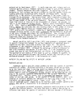 CT)
O)
-Q
f\
to
ITS
S-
cu
O)
">>
Q.
•r—
o.
O)
CO
o
T3
o
n3
3
•P
Q.
ai
o
c
o
o
oo
O)
Z5
cn
118
image:
CT)
O)
-Q
f\
to
ITS
S-
cu
O)
">>
Q.
•r—
o.
O)
CO
o
T3
o
n3
3
•P
Q.
ai
o
c
o
o
oo
O)
Z5
cn
118
image:
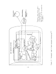 Energy source
Passive energy storage
Heat sink
Plant population
Self maintaining consumer population
Switch
Work gate
Figure 34. Energy language symbols (Odum 1972)
119
image:
Energy source
Passive energy storage
Heat sink
Plant population
Self maintaining consumer population
Switch
Work gate
Figure 34. Energy language symbols (Odum 1972)
119
image:
 in physical and chemical regimes. Phosphorus compounds in soils of low redox
potential, such as those found in the inundated root zone of aquatic plants, are
more soluble and more available than those found in aerobic soils. A marked
increase in extractable phosphorus was found in a soil profile ranging from a
redox potential of +200 mv to -200 mv which resulted from the transformation
of the ferric salt to the more reduced (and more soluble) ferrous phosphate
(Patrick andMahapatra 1968). The relative mobility of phosphorus is increased
in anoxic soils although little is known of the rate of transport to the over-
lying water (Syers et al. 1973).
Nitrogen mineralization in reducing conditions cannot proceed past the
formation of ammonium salts due to the absence of oxygen needed to convert to
nitrate. Rooted aquatics probably have adapted to this by selective uptake of
ammonium. Potamogeton alpinus was found to die when supplied nitrate as the
sole nitrogen source (Misra 1938). Other species may respond to nitrate,
however (Sculthorpe 1967). Ammonium ions tend to be bound to negatively charged
clay particles in the sediments although iffusion does occur. It is thought,
therefore, that the sediments function as a sink of phosphorus and nitrogen
and as a potential source for aquatic plants to draw on. The nutrient pool in
the water column can be accessed by submerged aquatic plants through the leaves
and stems. Submerged vascular plants act as nutrient traps and as a sink for
these dissolved minerals (Clark et al. 1973).
Submerged aquatic plants may serve as "nutrient pumps" in that the roots
can trap available nutrients and transport them to the pelagic zone. Inorganic
phosphate has been shown to be absorbed by the roots and translocated through-
out the plant (McRoy and Barsdate 1970; Bristow and Whitcombe 1971; McRoy et al.
1972; DeMarte and Hartman 1974) and may be excreted or "leaked" through the
leaves. The rate of transport may be light-dependent as shown by McRoy and
Barsdate (1970) with Zostera marina; however, DeMarte and Hartman (1974) found
no significant differences between light and dark translocation in Myriophyllutn
spicatum. If transport and release are affected by light, increased turbidity
and depth would decrease nutrient uptake and excretion. Leakage of phosphorus
may be considerable. Thirty-three percent of phosphate absorbed in the root
zone of Zostera marina was excreted from the plant (McRoy and Barsdate 1970).
DeMart and Hartman (1974) exhibited release of radioactive phosphate from
intact Myriophyllum spicatum, and the amount could be increased by physical
injury to the plant. However, working with the same species, Bristow and
Whitcombe (1971) found no leakage of phosphorus. Harlin (1973) showed a transfer
of inorganic phosphorus from Zostera marina to an algal epiphyte.
Nitrogen supplied to Z. marina roots in the N03~, NH^, and NH2(CO) forms
was translocated throughout the plant and excreted to an epiphytic community
(McRoy and Goering 1974). Iron and calcium were also found to be absorbed
from the sediment and released by the macrophyte Myriophyllum spicatum (DeMarte
and Hartman 1974).
In several freshwater aquatic species, inorganic carbon was taken up by
the roots and transported to the photosynthetic site (Wiurn-Anderson 1971).
This may also represent a mode of material transfer from the sediments.
120
image:
in physical and chemical regimes. Phosphorus compounds in soils of low redox
potential, such as those found in the inundated root zone of aquatic plants, are
more soluble and more available than those found in aerobic soils. A marked
increase in extractable phosphorus was found in a soil profile ranging from a
redox potential of +200 mv to -200 mv which resulted from the transformation
of the ferric salt to the more reduced (and more soluble) ferrous phosphate
(Patrick andMahapatra 1968). The relative mobility of phosphorus is increased
in anoxic soils although little is known of the rate of transport to the over-
lying water (Syers et al. 1973).
Nitrogen mineralization in reducing conditions cannot proceed past the
formation of ammonium salts due to the absence of oxygen needed to convert to
nitrate. Rooted aquatics probably have adapted to this by selective uptake of
ammonium. Potamogeton alpinus was found to die when supplied nitrate as the
sole nitrogen source (Misra 1938). Other species may respond to nitrate,
however (Sculthorpe 1967). Ammonium ions tend to be bound to negatively charged
clay particles in the sediments although iffusion does occur. It is thought,
therefore, that the sediments function as a sink of phosphorus and nitrogen
and as a potential source for aquatic plants to draw on. The nutrient pool in
the water column can be accessed by submerged aquatic plants through the leaves
and stems. Submerged vascular plants act as nutrient traps and as a sink for
these dissolved minerals (Clark et al. 1973).
Submerged aquatic plants may serve as "nutrient pumps" in that the roots
can trap available nutrients and transport them to the pelagic zone. Inorganic
phosphate has been shown to be absorbed by the roots and translocated through-
out the plant (McRoy and Barsdate 1970; Bristow and Whitcombe 1971; McRoy et al.
1972; DeMarte and Hartman 1974) and may be excreted or "leaked" through the
leaves. The rate of transport may be light-dependent as shown by McRoy and
Barsdate (1970) with Zostera marina; however, DeMarte and Hartman (1974) found
no significant differences between light and dark translocation in Myriophyllutn
spicatum. If transport and release are affected by light, increased turbidity
and depth would decrease nutrient uptake and excretion. Leakage of phosphorus
may be considerable. Thirty-three percent of phosphate absorbed in the root
zone of Zostera marina was excreted from the plant (McRoy and Barsdate 1970).
DeMart and Hartman (1974) exhibited release of radioactive phosphate from
intact Myriophyllum spicatum, and the amount could be increased by physical
injury to the plant. However, working with the same species, Bristow and
Whitcombe (1971) found no leakage of phosphorus. Harlin (1973) showed a transfer
of inorganic phosphorus from Zostera marina to an algal epiphyte.
Nitrogen supplied to Z. marina roots in the N03~, NH^, and NH2(CO) forms
was translocated throughout the plant and excreted to an epiphytic community
(McRoy and Goering 1974). Iron and calcium were also found to be absorbed
from the sediment and released by the macrophyte Myriophyllum spicatum (DeMarte
and Hartman 1974).
In several freshwater aquatic species, inorganic carbon was taken up by
the roots and transported to the photosynthetic site (Wiurn-Anderson 1971).
This may also represent a mode of material transfer from the sediments.
120
image:
 Rooted aquatic vascular plants are therefore capable of withdrawing mineral
nutrients from the anoxic zone and pumping them upward. Nutrients can also be
trapped from the water column and incorporated into biomass. Release of these
nutrients can occur by excretion by healthy plants or by the death and sub-
sequent decay of individuals.
Responses to Nutrient Loading
An increase of allochthonous nutrients into the aqueous system may produce
several effects on submerged vascular plants. With an increase of ambient
nutrient levels, levels within the plant will increase as well and may be
biologically concentrated (Anderson et al 1967; Allenby 1968). This may prove
to be a useful tool in the assessment of nutrient loading in that changes in
the chemical analysis of plant tissue would reflect changes in exterior levels
of nutrients (Sculthorpe 1967; Adams et al 1973). Changes in vegetative
morphology may occur as suggested by Adams et al. (1971) for El odea. Increases
in nutrient levels may also increase productivity in submerged species to a
certain point and several species have been shown to exhibit "luxury consumption"
(Orth, in press; Ryan 1969).
Phytosociological patterns may develop in response to nutrient levels.
Early workers (Pond 1905; Pearsall 1920; Misra 1938; Swindale and Curtis 1957)
found that the distribution of aquatic macrophytes was dependent on the chemical
nature of the substrate. Jaworski et al. (1972) using historical observations
of vegetation patterns in the Potomac River estuary, correlated increases in
nutrients with a succession of species. In their example, water chestnut
(Trapa natans) was replaced by Myriophyllum spicatum which was in turn replaced
by a cyanobacterial bloom of Anacystis. This succession was due to increases in
nitrogen and phosphorus and little correlation was found with changes in
available carbon. The same successional pattern was observed in rivers of the
upper Chesapeake Bay in response to nutrient loading (Clark et al. 1973). An
increase in phytoplankton in response to nutrient loading, as seen above, may
limit light and decrease productivities of macrophyte communities.
Predictions of the response of submerged vascular plants to nutrient
loading based on present knowledge would be equivocal. More research is necessary
if answers to these questions are to ascertained.
SUBMERGED AQUATIC MACROPHYTES AS BIO-INDICATORS
Submerged aquatic species are not commonly viewed as indicators of
biological conditions or trends within the Chesapeake Bay. The aquatic grasses
do not respond as rapidly to environmental conditions as various algal, phyto-
plankton and zooplankton species that are capable of rapid growth in bloom
proportions.
Sculthorpe (1967) suggested that SAV species are potentially useful as
indicators of pollution trends. Adams et al. (1971) supported Sculthorpe's
suggestion with evidence as to chemical and morphological responses of El odea
canadensis to increasing levels of nutrient pollution. As of their writing,
Adams et al. indicated that no experimentally comprehensive work had been
performed in order to evaluate the potential advantages or disadvantages
121
image:
Rooted aquatic vascular plants are therefore capable of withdrawing mineral
nutrients from the anoxic zone and pumping them upward. Nutrients can also be
trapped from the water column and incorporated into biomass. Release of these
nutrients can occur by excretion by healthy plants or by the death and sub-
sequent decay of individuals.
Responses to Nutrient Loading
An increase of allochthonous nutrients into the aqueous system may produce
several effects on submerged vascular plants. With an increase of ambient
nutrient levels, levels within the plant will increase as well and may be
biologically concentrated (Anderson et al 1967; Allenby 1968). This may prove
to be a useful tool in the assessment of nutrient loading in that changes in
the chemical analysis of plant tissue would reflect changes in exterior levels
of nutrients (Sculthorpe 1967; Adams et al 1973). Changes in vegetative
morphology may occur as suggested by Adams et al. (1971) for El odea. Increases
in nutrient levels may also increase productivity in submerged species to a
certain point and several species have been shown to exhibit "luxury consumption"
(Orth, in press; Ryan 1969).
Phytosociological patterns may develop in response to nutrient levels.
Early workers (Pond 1905; Pearsall 1920; Misra 1938; Swindale and Curtis 1957)
found that the distribution of aquatic macrophytes was dependent on the chemical
nature of the substrate. Jaworski et al. (1972) using historical observations
of vegetation patterns in the Potomac River estuary, correlated increases in
nutrients with a succession of species. In their example, water chestnut
(Trapa natans) was replaced by Myriophyllum spicatum which was in turn replaced
by a cyanobacterial bloom of Anacystis. This succession was due to increases in
nitrogen and phosphorus and little correlation was found with changes in
available carbon. The same successional pattern was observed in rivers of the
upper Chesapeake Bay in response to nutrient loading (Clark et al. 1973). An
increase in phytoplankton in response to nutrient loading, as seen above, may
limit light and decrease productivities of macrophyte communities.
Predictions of the response of submerged vascular plants to nutrient
loading based on present knowledge would be equivocal. More research is necessary
if answers to these questions are to ascertained.
SUBMERGED AQUATIC MACROPHYTES AS BIO-INDICATORS
Submerged aquatic species are not commonly viewed as indicators of
biological conditions or trends within the Chesapeake Bay. The aquatic grasses
do not respond as rapidly to environmental conditions as various algal, phyto-
plankton and zooplankton species that are capable of rapid growth in bloom
proportions.
Sculthorpe (1967) suggested that SAV species are potentially useful as
indicators of pollution trends. Adams et al. (1971) supported Sculthorpe's
suggestion with evidence as to chemical and morphological responses of El odea
canadensis to increasing levels of nutrient pollution. As of their writing,
Adams et al. indicated that no experimentally comprehensive work had been
performed in order to evaluate the potential advantages or disadvantages
121
image:
 relating to the use of SAV as aquatic pollution trend indicators. They further
suggested the need for clarification as to the identification of specific
nutrient pollution conditions in relation to individual SAV species.
In assessing the value of using plants as indicators in place of modern
water pollution analysis technology, Adams et al.(1971) pointed out that relative
costs, scope and manpower requirements should be compared. They concluded that
automated monitoring systems are initially costly, expensive to maintain and
limited in scope. By comparison, water monitoring through the use of pollution-
sensitive SAV would not only reduce initial and maintenance costs but could
provide a wide coverage using essentially a single instrument. Adams et al.
suggested a system of transporting trfays of stock plants to various locations
and the selective breeding of species sensitive to specific pollutants.
The floating aquatic duckweed (Lemna perpusilla) has been used by Feder
and Sullivan (1969, abstracted in Thomas et al. 1973) in experiments with
ozone. Plants treated with a low concentration of ozone over two weeks were
slower to multiply, had a lower rate of frond doubling and were slower to
produce fewer flowers than control plants.
Several species of submerged and floating macrophytes have been tested for
effects from smelter pollution in Ontario (Gorham and Gordon 1963 , abstracted
in Thomas et al. 1973). Species occurrence was found to be inversely related to
dissolved sulphate. Species diversity was low even where sulphuric acid was
almost totally neutralized and waters were above pH 6. Utricularia vulgaris
and Potamogeton epihydrus v. nuttallii appeared to be rather sensitive to heavy
metal concentration.
Burrows (1971, abstracted in Thomas et al. 1973) indicates that Ulva
lactuca has potential as a pollution indicator species because of its ease of
culture and sewage pollution reactions. Laminaria saccharina is also listed as
a possible indicator species due to its sensitivity and availability. An
historic view of eutrophication in the Potomac River estuary (Jaworski et al.1972)
suggests that nuisance plant conditions did not develop linearly with an increase
in nutrients. As nutrient loading increased in the estuary, nuisance plant
growth was favored based on individual species nutrient requirements. Thus,
Trapa natans infested the Potomac in the 1920s to be replaced by Myriophyllum
spicatum in the 1950s and 1960s. As milfoil died out in the mid 1960s, it
was replaced by the blue-green alga Anacystis. The massive blooms of Anacystis
that have occurred each summer since 1960 can be associated with phosphorus and
nitrogen loading increases.
TURBIDITY AND WATER MOVEMENT
Submerged aquatic plants tend to modify their physical environment through
their growth habits. By providing resistance to stream flow and wave action,
hydrophytes not only reduce average water movement but aid in the settling out
of silt particles thus reducing turbidity and building up substrates.
(Sculthorpe 1967) Macrophytes initially provide frictional resistance to current
velocity.
122
image:
relating to the use of SAV as aquatic pollution trend indicators. They further
suggested the need for clarification as to the identification of specific
nutrient pollution conditions in relation to individual SAV species.
In assessing the value of using plants as indicators in place of modern
water pollution analysis technology, Adams et al.(1971) pointed out that relative
costs, scope and manpower requirements should be compared. They concluded that
automated monitoring systems are initially costly, expensive to maintain and
limited in scope. By comparison, water monitoring through the use of pollution-
sensitive SAV would not only reduce initial and maintenance costs but could
provide a wide coverage using essentially a single instrument. Adams et al.
suggested a system of transporting trfays of stock plants to various locations
and the selective breeding of species sensitive to specific pollutants.
The floating aquatic duckweed (Lemna perpusilla) has been used by Feder
and Sullivan (1969, abstracted in Thomas et al. 1973) in experiments with
ozone. Plants treated with a low concentration of ozone over two weeks were
slower to multiply, had a lower rate of frond doubling and were slower to
produce fewer flowers than control plants.
Several species of submerged and floating macrophytes have been tested for
effects from smelter pollution in Ontario (Gorham and Gordon 1963 , abstracted
in Thomas et al. 1973). Species occurrence was found to be inversely related to
dissolved sulphate. Species diversity was low even where sulphuric acid was
almost totally neutralized and waters were above pH 6. Utricularia vulgaris
and Potamogeton epihydrus v. nuttallii appeared to be rather sensitive to heavy
metal concentration.
Burrows (1971, abstracted in Thomas et al. 1973) indicates that Ulva
lactuca has potential as a pollution indicator species because of its ease of
culture and sewage pollution reactions. Laminaria saccharina is also listed as
a possible indicator species due to its sensitivity and availability. An
historic view of eutrophication in the Potomac River estuary (Jaworski et al.1972)
suggests that nuisance plant conditions did not develop linearly with an increase
in nutrients. As nutrient loading increased in the estuary, nuisance plant
growth was favored based on individual species nutrient requirements. Thus,
Trapa natans infested the Potomac in the 1920s to be replaced by Myriophyllum
spicatum in the 1950s and 1960s. As milfoil died out in the mid 1960s, it
was replaced by the blue-green alga Anacystis. The massive blooms of Anacystis
that have occurred each summer since 1960 can be associated with phosphorus and
nitrogen loading increases.
TURBIDITY AND WATER MOVEMENT
Submerged aquatic plants tend to modify their physical environment through
their growth habits. By providing resistance to stream flow and wave action,
hydrophytes not only reduce average water movement but aid in the settling out
of silt particles thus reducing turbidity and building up substrates.
(Sculthorpe 1967) Macrophytes initially provide frictional resistance to current
velocity.
122
image:
 Some species of macrophytes, ideally those SAV with linear ribbon-like
leaves do not provide finely dissected surfaces that trap silt particles and
organisms. Thus particulate matter settles, becomes established and provides
bottom sediments that are often conducive to the establishment of further SAV.
Further colonization results in yet slower currents and greater sediment
deposition (Mitchell 1974). Sculthorpe (1967) cited Millebrand (1950) as having
found a 75 percent reduction in maximum current velocity in SAV colonized river
areas.
SEDIMENT STABILIZATION
High energy shorelines are not conducive to colonization by SAV. However,
in areas where vegetation is established, grass beds aid in the deposition and
stabilization of bottom sediments. As plants provide resistance to currents,
particulate matter settles and builds up a substrate of fine silt particles
that enhances plant colonization. As plant root stock developes and the SAV
beds expand, bottom substrates are further stabilized.
PH
Hydrogen ion concentration, or pH in an aquatic environment, is a function
of the dissolved C02 content; as the C02 content is lowered, pH increases. Thus
as plants photosynthesize during the day and lower the dissolved C02, the pH
will increase. At night as plants respire and give off C02, the pH will decrease.
The degree of change in pH is greatly determined by the buffering capacity
of the aquatic medium. Carbon dioxide combines with water to form H2C03 which
in turn reacts with limestone to form carbonates (-C03) and bicarbonates (HCOs).
This carbon dioxide-carbonate-bicarbonate complex acts as a buffer and results
in more neutral conditions.
Aquatic plants thus affect pH through C02 fluctuations and pH in turn
affects plant chemical processes. Enzyme activity rate has been determined to
be influenced by the pH of the medium as enzymes exhibit optimum activity
within specific pH ranges (Small 1946). pH further influences imbibition or
swelling of prbteins and is thus related to seed germination. Hydrogen ion
concentration may alter heat susceptibility and enzyme solubility and is related
to absorption and accumulation of salts (Curtis and Clark 1950). Toxicity
and solubility of heavy metals, detergents, aromatic solvents, acids, alkalis
and salts may also be influenced by pH (Sculthorpe 1967).
COMMERCIAL AND CONSERVATION VALUES
In various parts of the world, species of submerged aquatic vegetation are
considered a resource and used for forage and fertilizer. Commission on Inter-
national Relations (1976) includes such examples as the use of water hyacinth
(Eichornia spp») for bedding material in mushroom cultivation in the Philippines,
as a substitute for German peat moss, as a propagation medium for houseplants
and as a nutritional supplement for nonruminant animals in Southeast Asia.
123
image:
Some species of macrophytes, ideally those SAV with linear ribbon-like
leaves do not provide finely dissected surfaces that trap silt particles and
organisms. Thus particulate matter settles, becomes established and provides
bottom sediments that are often conducive to the establishment of further SAV.
Further colonization results in yet slower currents and greater sediment
deposition (Mitchell 1974). Sculthorpe (1967) cited Millebrand (1950) as having
found a 75 percent reduction in maximum current velocity in SAV colonized river
areas.
SEDIMENT STABILIZATION
High energy shorelines are not conducive to colonization by SAV. However,
in areas where vegetation is established, grass beds aid in the deposition and
stabilization of bottom sediments. As plants provide resistance to currents,
particulate matter settles and builds up a substrate of fine silt particles
that enhances plant colonization. As plant root stock developes and the SAV
beds expand, bottom substrates are further stabilized.
PH
Hydrogen ion concentration, or pH in an aquatic environment, is a function
of the dissolved C02 content; as the C02 content is lowered, pH increases. Thus
as plants photosynthesize during the day and lower the dissolved C02, the pH
will increase. At night as plants respire and give off C02, the pH will decrease.
The degree of change in pH is greatly determined by the buffering capacity
of the aquatic medium. Carbon dioxide combines with water to form H2C03 which
in turn reacts with limestone to form carbonates (-C03) and bicarbonates (HCOs).
This carbon dioxide-carbonate-bicarbonate complex acts as a buffer and results
in more neutral conditions.
Aquatic plants thus affect pH through C02 fluctuations and pH in turn
affects plant chemical processes. Enzyme activity rate has been determined to
be influenced by the pH of the medium as enzymes exhibit optimum activity
within specific pH ranges (Small 1946). pH further influences imbibition or
swelling of prbteins and is thus related to seed germination. Hydrogen ion
concentration may alter heat susceptibility and enzyme solubility and is related
to absorption and accumulation of salts (Curtis and Clark 1950). Toxicity
and solubility of heavy metals, detergents, aromatic solvents, acids, alkalis
and salts may also be influenced by pH (Sculthorpe 1967).
COMMERCIAL AND CONSERVATION VALUES
In various parts of the world, species of submerged aquatic vegetation are
considered a resource and used for forage and fertilizer. Commission on Inter-
national Relations (1976) includes such examples as the use of water hyacinth
(Eichornia spp») for bedding material in mushroom cultivation in the Philippines,
as a substitute for German peat moss, as a propagation medium for houseplants
and as a nutritional supplement for nonruminant animals in Southeast Asia.
123
image:
 Boyd (1974) discussed the food value of several emergent and submergent aquatic
plants including Najas guadalupensis, Ceratophyllurn demersum and Potampgeton
diversifolium. Table 18 compares these three SAV with alfalfa.
Table 18. Food value (percent dry weight) of several species of
submerged aquatic vegetation and alfalfa3
Crude
Ash Protein Cellulose
Species % % Fat %
Najas guadalupensis
Ceratophyllum demersum
Potamogeton diversifolius
Eichornia crass ipes
Alfalfa
18.7
20.6
22.7
18.0
8.6
22.8
21.7
17.3
17.1
18.6
3.8
6.0
2.8
3.6
2.6
35.6
27.9
30.9
28.2
23.7
a Boyd 1974
Despite the high nutritive levels in some SAV species, they also have a high
water content. In order to best use the plant material for fodder, the 90 to
95 percent water content should be lowered by dehydration in order to increase
the food value per weight. This need for drying increases the expense and
decreases the practicality of using SAV for fodder (Boyd 1974).
In the United States, the National Aeronautics and Space Administration
(NASA) is conducting research on the use of water hyacinth and other aquatic
plants as a source of methane gas. Also being investigated is the use of such
SAV species as Elodea canadensis and Ceratophyllum demersum in water-treatment
systems (Commission on International Relations 1976). Water hyacinth is already
being used in Lucedale, Mississippi, by a NASA facility to remove nutrients from
sewage effluent (Commission on International Relations 1976). The harvested
plant material is then processed for animal feed, fuel and fertilizer. Duckweed
(Spirodela sp.) is being grown at Louisiana State University on dairy farm
effluents then substituted for alfalfa for swine and dairy feed (Commission on
International Relations 1976).
Native submerged aquatic vegetation in the Chesapeake Bay is generally
regarded more for its beneficial use by wildlife than its possible commercial use.
Field work is presently being conducted by Vernon Stotts, Maryland Wildlife
Administration to determine the feasibility and success of planting methods for
Ruppia maritima. Further work on this variety would be necessary in order to
establish the usefulness of SAV in the establishment of conservation areas, the
possible use of SAV as bio-indicators and the feasibility of commercial SAV uses.
124
image:
Boyd (1974) discussed the food value of several emergent and submergent aquatic
plants including Najas guadalupensis, Ceratophyllurn demersum and Potampgeton
diversifolium. Table 18 compares these three SAV with alfalfa.
Table 18. Food value (percent dry weight) of several species of
submerged aquatic vegetation and alfalfa3
Crude
Ash Protein Cellulose
Species % % Fat %
Najas guadalupensis
Ceratophyllum demersum
Potamogeton diversifolius
Eichornia crass ipes
Alfalfa
18.7
20.6
22.7
18.0
8.6
22.8
21.7
17.3
17.1
18.6
3.8
6.0
2.8
3.6
2.6
35.6
27.9
30.9
28.2
23.7
a Boyd 1974
Despite the high nutritive levels in some SAV species, they also have a high
water content. In order to best use the plant material for fodder, the 90 to
95 percent water content should be lowered by dehydration in order to increase
the food value per weight. This need for drying increases the expense and
decreases the practicality of using SAV for fodder (Boyd 1974).
In the United States, the National Aeronautics and Space Administration
(NASA) is conducting research on the use of water hyacinth and other aquatic
plants as a source of methane gas. Also being investigated is the use of such
SAV species as Elodea canadensis and Ceratophyllum demersum in water-treatment
systems (Commission on International Relations 1976). Water hyacinth is already
being used in Lucedale, Mississippi, by a NASA facility to remove nutrients from
sewage effluent (Commission on International Relations 1976). The harvested
plant material is then processed for animal feed, fuel and fertilizer. Duckweed
(Spirodela sp.) is being grown at Louisiana State University on dairy farm
effluents then substituted for alfalfa for swine and dairy feed (Commission on
International Relations 1976).
Native submerged aquatic vegetation in the Chesapeake Bay is generally
regarded more for its beneficial use by wildlife than its possible commercial use.
Field work is presently being conducted by Vernon Stotts, Maryland Wildlife
Administration to determine the feasibility and success of planting methods for
Ruppia maritima. Further work on this variety would be necessary in order to
establish the usefulness of SAV in the establishment of conservation areas, the
possible use of SAV as bio-indicators and the feasibility of commercial SAV uses.
124
image:
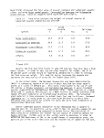 CHAPTER 3
HISTORICAL TRENDS OF CHESAPEAKE BAY SUBMERGED AQUATICS
INTRODUCTION
Historic documentation of the distribution and abundance of aquatic vege-
tation in the Chesapeake Bay is sparse until the late 1950s. Up to that time,
documentation is limited primarily to occasional newspaper references, herbarium
notations, personal communications and occasional scientific papers dealing with
single-season populations found in specific areas. The oldest records available
are found in the Smithsonian's herbarium dating back to 1871. From the late
1920s through the present, Francis Uhler of the U.S. Fish and Wildlife Service
Migratory Bird and Habitat Research Laboratory (MBHRL), has observed and noted
Bay grasses, especially in the Potomac River.
The first comprehensive survey of SAV was begun in 1958 on the Susquehanna
Flats by MBHRL personnel. Located in the upper Bay at the mouth of the
Susquehanna River, this area has always been important for waterfowl feeding.
This study is presently being continued and documents the occurrence and relative
abundance of all the major species of SAV on the Flats.
In 1959, Vernon Stotts of the Maryland Wildlife Administration designed
a transect system for sampling Maryland Chesapeake Bay benthos in the autumn
(Maryland Pittman-Robertson Project W-30-R-8). Based on nine transect lines,
this Benthic Survey was continued through 1961.
In 1967, Vernon Stotts again designed a summer vegetation sampling program
(Maryland Pittman-Robertson Project W-45-2). This survey dealt only with SAV
and was based on an intensive network of transects radiating from the shorelines.
The Vegetation Survey covered the Maryland Eastern Shore and was continued
through 1969.
The idea of this survey was picked up by James A. Kerwin and Robert E.
Munro of the MBHRL and summer sampling began in 1971 with the aid of Vernon
Stotts. This survey is presently in operation and is the only Maryland Bay-wide
program in existence for rooted aquatics.
Available information for SAV in Virginia waters is limited mainly to herbarium
specimens and the work of Robert Orth and Walter Priest from Virginia Institute
of Marine Science. Orth has studied extensively the history of Zostera marina
in the Bay as well as searching literature on the world-wide distribution and
abundance of eel grass. Priest surveyed the Rappahannock and Piankatank Rivers
125
image:
CHAPTER 3
HISTORICAL TRENDS OF CHESAPEAKE BAY SUBMERGED AQUATICS
INTRODUCTION
Historic documentation of the distribution and abundance of aquatic vege-
tation in the Chesapeake Bay is sparse until the late 1950s. Up to that time,
documentation is limited primarily to occasional newspaper references, herbarium
notations, personal communications and occasional scientific papers dealing with
single-season populations found in specific areas. The oldest records available
are found in the Smithsonian's herbarium dating back to 1871. From the late
1920s through the present, Francis Uhler of the U.S. Fish and Wildlife Service
Migratory Bird and Habitat Research Laboratory (MBHRL), has observed and noted
Bay grasses, especially in the Potomac River.
The first comprehensive survey of SAV was begun in 1958 on the Susquehanna
Flats by MBHRL personnel. Located in the upper Bay at the mouth of the
Susquehanna River, this area has always been important for waterfowl feeding.
This study is presently being continued and documents the occurrence and relative
abundance of all the major species of SAV on the Flats.
In 1959, Vernon Stotts of the Maryland Wildlife Administration designed
a transect system for sampling Maryland Chesapeake Bay benthos in the autumn
(Maryland Pittman-Robertson Project W-30-R-8). Based on nine transect lines,
this Benthic Survey was continued through 1961.
In 1967, Vernon Stotts again designed a summer vegetation sampling program
(Maryland Pittman-Robertson Project W-45-2). This survey dealt only with SAV
and was based on an intensive network of transects radiating from the shorelines.
The Vegetation Survey covered the Maryland Eastern Shore and was continued
through 1969.
The idea of this survey was picked up by James A. Kerwin and Robert E.
Munro of the MBHRL and summer sampling began in 1971 with the aid of Vernon
Stotts. This survey is presently in operation and is the only Maryland Bay-wide
program in existence for rooted aquatics.
Available information for SAV in Virginia waters is limited mainly to herbarium
specimens and the work of Robert Orth and Walter Priest from Virginia Institute
of Marine Science. Orth has studied extensively the history of Zostera marina
in the Bay as well as searching literature on the world-wide distribution and
abundance of eel grass. Priest surveyed the Rappahannock and Piankatank Rivers
125
image:
 in the spring of 1977. Preliminary results of the 1977 MBHRL Survey of the
Potomac River have been included in the conclusion section of this chapter.
these data are for both Maryland and Virginia,
These surveys constitute the main body of available knowledge on the dis-
tribution of SAV in the Bay. Along with site-specific studies, herbaria speci-
mens, newspaper accounts and personal communications, the findings of the
surveys will be presented later in this chapter.
CHESAPEAKE BAY CHRONOLOGY
In attempting to assess an historic documentation of declines in submerged
aquatic vegetation in the Chesapeake Bay, it is first necessary to view the
situation chronologically. Table 19 presents almost fifty years of Bay area
history including major storms,droughts, population growth, pest plant infesta-
tions and abnormal precipitation levels. The following section discusses many
of these major events and their immediate results.
1920s
Water chestnut (Trapa natans) first appeared near the mouth of Oxon Run
at the head of the Potomac River in 1923 (Rawls 1964). Within a decade, the
species had spread over forty miles of the river in shallow water areas. Water-
fowl breeding grounds were termed useless (Maryland Department of Tidewater
Fisheries 1955) presumably because milfoil is generally considered to be one of
the least desirable waterfowl foods.
1930s
In the early 1930s, Francis Uhler, MBHRL is reported to having seen ducks
feeding on redhead grass and wild celery from the old 14th Street Bridge in
Washington, D. C. (Rawls et al. 1975).
On August 23, 1933, the Bay was hit by the century's worst storm. Water
rose about 45 cm per hour sending 0.6 to 0.9 m high waves over land
and resulting in 6 to 9 m high waves in the ocean. The water level was
almost three feet higher than the "great centennial" storm of 1876 (Daily Banner),
August 25, 1933).
On September 16, 1933, another storm hit, raising water levels to similar
heights as the storm of the previous month. The Daily Banner reported September
20, 1933, that thousands of tons of eel grass and peat plants were destroyed in
the Nanticoke, Blackwater and Hooper Island area by excessive wave action.
From 1930 to 1932, an unprecedented drought brought brackish water farther
up into the estuaries (Stewart 1962). This impact, coupled with the crowding
out effects of an increasing abundance of Trapa natarrs, caused SAV to gradually
disappear by 1935 (Gwathmey 1945; Stewart 1962). The impact of the drought
followed by the 1933 storms contributed to about five years of severe biological
stress to the Chesapeake Bay ecosystem.
126
image:
in the spring of 1977. Preliminary results of the 1977 MBHRL Survey of the
Potomac River have been included in the conclusion section of this chapter.
these data are for both Maryland and Virginia,
These surveys constitute the main body of available knowledge on the dis-
tribution of SAV in the Bay. Along with site-specific studies, herbaria speci-
mens, newspaper accounts and personal communications, the findings of the
surveys will be presented later in this chapter.
CHESAPEAKE BAY CHRONOLOGY
In attempting to assess an historic documentation of declines in submerged
aquatic vegetation in the Chesapeake Bay, it is first necessary to view the
situation chronologically. Table 19 presents almost fifty years of Bay area
history including major storms,droughts, population growth, pest plant infesta-
tions and abnormal precipitation levels. The following section discusses many
of these major events and their immediate results.
1920s
Water chestnut (Trapa natans) first appeared near the mouth of Oxon Run
at the head of the Potomac River in 1923 (Rawls 1964). Within a decade, the
species had spread over forty miles of the river in shallow water areas. Water-
fowl breeding grounds were termed useless (Maryland Department of Tidewater
Fisheries 1955) presumably because milfoil is generally considered to be one of
the least desirable waterfowl foods.
1930s
In the early 1930s, Francis Uhler, MBHRL is reported to having seen ducks
feeding on redhead grass and wild celery from the old 14th Street Bridge in
Washington, D. C. (Rawls et al. 1975).
On August 23, 1933, the Bay was hit by the century's worst storm. Water
rose about 45 cm per hour sending 0.6 to 0.9 m high waves over land
and resulting in 6 to 9 m high waves in the ocean. The water level was
almost three feet higher than the "great centennial" storm of 1876 (Daily Banner),
August 25, 1933).
On September 16, 1933, another storm hit, raising water levels to similar
heights as the storm of the previous month. The Daily Banner reported September
20, 1933, that thousands of tons of eel grass and peat plants were destroyed in
the Nanticoke, Blackwater and Hooper Island area by excessive wave action.
From 1930 to 1932, an unprecedented drought brought brackish water farther
up into the estuaries (Stewart 1962). This impact, coupled with the crowding
out effects of an increasing abundance of Trapa natarrs, caused SAV to gradually
disappear by 1935 (Gwathmey 1945; Stewart 1962). The impact of the drought
followed by the 1933 storms contributed to about five years of severe biological
stress to the Chesapeake Bay ecosystem.
126
image:
 Table 19. Chesapeake Bay chronology
1930 1930's Trapa natans infestation in Upper Potomac River; 1930's
Zostera decline
1931 Severe drought
1932 Hurricane (August) -- extreme tides
1934 Residual severe biological stress from 1933
1935
1936 Record flood (March)
1937
1938
1939
1940 Bay area population 1,600,000
1941
1942 Flood (October)
1943
1944
1945
1946
1947
1948
1949
1950 Approximately 4,000 ha of Potomac infested with Trapa natans
1951
1952
1953
1954 Hurrican Hazel (October)
1955 Tropical storm Connie (August); tropical storm Diane (August)
1956 Northeastern (April)
1957 One-third 1958 rainfall (May to August)
1958
1959
1960 Tropical storm Donna (September); Bay area population 2,600,000
1961 Approximately 20,000 ha of Bay covered with Myriophyllum
1962 Northeastern (March); over 40,000 ha of Bay covered with Myriophyllum
1963 Drought from 1963 to 1965
1964 Salt water intrusion from 1964 to 1966; drought
1965 Drought
1966
1967 Excessive precipitation (May and June)
1968
1969 Abnormally low precipitation (winter); high precipitation (summer)
1970 Bay area population 3,100,000
1971
1972 Tropical storm Agnes (June)
1973
1974
1975
1976 Exceptionally low precipitation
1977 Record cold winter
127
image:
Table 19. Chesapeake Bay chronology
1930 1930's Trapa natans infestation in Upper Potomac River; 1930's
Zostera decline
1931 Severe drought
1932 Hurricane (August) -- extreme tides
1934 Residual severe biological stress from 1933
1935
1936 Record flood (March)
1937
1938
1939
1940 Bay area population 1,600,000
1941
1942 Flood (October)
1943
1944
1945
1946
1947
1948
1949
1950 Approximately 4,000 ha of Potomac infested with Trapa natans
1951
1952
1953
1954 Hurrican Hazel (October)
1955 Tropical storm Connie (August); tropical storm Diane (August)
1956 Northeastern (April)
1957 One-third 1958 rainfall (May to August)
1958
1959
1960 Tropical storm Donna (September); Bay area population 2,600,000
1961 Approximately 20,000 ha of Bay covered with Myriophyllum
1962 Northeastern (March); over 40,000 ha of Bay covered with Myriophyllum
1963 Drought from 1963 to 1965
1964 Salt water intrusion from 1964 to 1966; drought
1965 Drought
1966
1967 Excessive precipitation (May and June)
1968
1969 Abnormally low precipitation (winter); high precipitation (summer)
1970 Bay area population 3,100,000
1971
1972 Tropical storm Agnes (June)
1973
1974
1975
1976 Exceptionally low precipitation
1977 Record cold winter
127
image:
 By 1933, 4,000 ha of Trapa natans thrived in the Potamac River from
Quantico north, to the falls. Satisfactory control was achieved through under-
water mowing techniques by the U.S. Army Corps of Engineers (Rawls 1964).
Along the east coast of North America and the west coast of Europe, major
declines in Zostera occurred in the 1930s. The causal organism may have been
the protozoan, Labyrinthula. Discussions as to the decline of eelgrass are
presented in Chapter 1 in the section dealing with Zostera marina and in Chapter
4 in the section on diseases.
1950s
Hurricane Hazel hit the Eastern Shore on October 5, 1954, with 161 kph
winds and 45 m waves (Daily Banner, October 15, 1954). Farm pastures
and agricultural land was destroyed by salt water (Daily Banner, October 20,
1954). It was estimated that from 2,200 to 11,000 kg/ha salt was deposited on
the fields (Daily Banner, November 4, 1954). Captain Amos Creighton, Department
of Tidewater Fisheries, surveyed Eastern Shore oyster beds and found little
damage (Daily Banner, October 22, 1954). The Compass (Maryland Department of
Tidewater Fisheries, December, 1954) reported that the grass beds did not seem
to be damaged even though the storm was the worst one since August 23, 1933.
Within three years after Hurricane Hazel and tropical storms Connie and Diane
(1955), aquatic plant populations in the Bay were termed luxuriant (Springer
et al. 1958),
Invasion of the upper Chesapeake Bay by Eurasian watermilfoil (Myriophyllum
spicatum) became apparent in 1954 when plants were discovered in the Gunpowder
River (Steenis et al. 1962). By 1958, Myriophyllum was becoming a very serious
pest plant. Chesapeake Bay Laboratory, Virginia Institute of Marine Science
and MBHRL had begun to receive complaints and aid requests from property owners,
and sport, civic and commercial groups. Creeks and small rivers where choked
with milfoil mats that prevented navigation (Rawls 1964).
Waterchestnut infestation became a serious problem again in 1950 with ap-
proximately 72 km of the Potomac River covered with the species. The River and
Harbor Act of May 17, 1950, provided authorization for the complete eradication
of Trapa from the Potomac River and tributaties (Kolessar 1967)
1960s
By 1961, an estimated 20,200 ha of tidewater Maryland were infested with
Myriophy11umH In the summer of the following year, over 40,500 ha were covered
(Rawls 1964). On the Susquehanna Flats alone, autumn surveys in 1960 documented
milfoil at 84 percent of the 60 to 80 stations surveyed (Stotts 1961).
In June of 1967, continuous excessive precipitation caused a "wash-in" of
muddy water. Though this condition was probably not solely at fault, it seemed
to be instrumental in bringing about a noticeable reduction of SAV to scattered
pockets of vegetation in the fresh and brackish portions of the Bay (Steenis
1970).
128
image:
By 1933, 4,000 ha of Trapa natans thrived in the Potamac River from
Quantico north, to the falls. Satisfactory control was achieved through under-
water mowing techniques by the U.S. Army Corps of Engineers (Rawls 1964).
Along the east coast of North America and the west coast of Europe, major
declines in Zostera occurred in the 1930s. The causal organism may have been
the protozoan, Labyrinthula. Discussions as to the decline of eelgrass are
presented in Chapter 1 in the section dealing with Zostera marina and in Chapter
4 in the section on diseases.
1950s
Hurricane Hazel hit the Eastern Shore on October 5, 1954, with 161 kph
winds and 45 m waves (Daily Banner, October 15, 1954). Farm pastures
and agricultural land was destroyed by salt water (Daily Banner, October 20,
1954). It was estimated that from 2,200 to 11,000 kg/ha salt was deposited on
the fields (Daily Banner, November 4, 1954). Captain Amos Creighton, Department
of Tidewater Fisheries, surveyed Eastern Shore oyster beds and found little
damage (Daily Banner, October 22, 1954). The Compass (Maryland Department of
Tidewater Fisheries, December, 1954) reported that the grass beds did not seem
to be damaged even though the storm was the worst one since August 23, 1933.
Within three years after Hurricane Hazel and tropical storms Connie and Diane
(1955), aquatic plant populations in the Bay were termed luxuriant (Springer
et al. 1958),
Invasion of the upper Chesapeake Bay by Eurasian watermilfoil (Myriophyllum
spicatum) became apparent in 1954 when plants were discovered in the Gunpowder
River (Steenis et al. 1962). By 1958, Myriophyllum was becoming a very serious
pest plant. Chesapeake Bay Laboratory, Virginia Institute of Marine Science
and MBHRL had begun to receive complaints and aid requests from property owners,
and sport, civic and commercial groups. Creeks and small rivers where choked
with milfoil mats that prevented navigation (Rawls 1964).
Waterchestnut infestation became a serious problem again in 1950 with ap-
proximately 72 km of the Potomac River covered with the species. The River and
Harbor Act of May 17, 1950, provided authorization for the complete eradication
of Trapa from the Potomac River and tributaties (Kolessar 1967)
1960s
By 1961, an estimated 20,200 ha of tidewater Maryland were infested with
Myriophy11umH In the summer of the following year, over 40,500 ha were covered
(Rawls 1964). On the Susquehanna Flats alone, autumn surveys in 1960 documented
milfoil at 84 percent of the 60 to 80 stations surveyed (Stotts 1961).
In June of 1967, continuous excessive precipitation caused a "wash-in" of
muddy water. Though this condition was probably not solely at fault, it seemed
to be instrumental in bringing about a noticeable reduction of SAV to scattered
pockets of vegetation in the fresh and brackish portions of the Bay (Steenis
1970).
128
image:
 1970s
Hurricane Agnes reached the Chesapeake Bay on June 21, 1972, after an
unusually wet winter and spring. Over a three-day period from 19 to 45 cm
of rain was dumped on various portions of the Bay watershed. Documented
results of the subsequent flooding include impacts to; salinity regimes;
sedimentation rates; dissolved phosphorus and nitrogen levels; trace metal
and pesticide budgets; dissolved oxygen content; shellfish; aquatic plants;
plankton; and benthos. Economic impact was assessed at $43 million distri-
buted mainly on the Western Shore in the shellfishing, tourism and recreation
industries in both Maryland and Virginia (Davis 1974).
Bayley et al. (in press) indicated that submerged aquatic plant recovery
had been slower than after the storms of the 1950s. Also after Agnes they
reported that dominant aquatic plant species in the Susquehanna Flats no longer
grew at the deeper depths as during the early 1960s.
DOCUMENTATION SURVEYS
Documentation surveys vary widely as to geographic coverage, season, year,
sampling method, data analysis and purpose. The only common denominator is
species occurrence.
The two most important variables that affect the individual surveys results
are season and data quantification. The time of year in which a survey is
performed will greatly affect the results. Some species, for example
ZannicheTMa palustris, exhibits two growing seasons, one in the spring and
another in the fall. Therefore, a survey performed during July and August,
such as the MBHRL Survey, would not document as much Z_. palustris as a survey
done in May or June or in the fall.
In comparing some surveys, data quantification becomes a problem of
semantics. The commonly used terms of "abundant", "common" and "rare" sometimes
refer to visual estimates and other times refer to volumetric analysis. Visual
estimates are highly subjective and at times are based on the percent of a
grab sample or the density of a quadrat. Other times the assessment is made
according to relative abundance among species.
Survey data is presented in this chapter to the degree of analysis avail-
able in the original work. However, conclusions based on the body of informa-
tion available by combining all surveys has been limited primarily to species
occurrence due to the analysis problems just described.
General conclusions and possible trends based on these surveys are pre-
sented and analyzed in Chapter 4 in relation to the environmental parameters
that are known to affect submerged aquatic vegetation.
Susquehanna Flats Survey, 1958 - present
The first major study of rooted aquatics was conceived in 1957 to study
the effects of hurricanes on the Susquehanna Flats. Paul Springer,
129
image:
1970s
Hurricane Agnes reached the Chesapeake Bay on June 21, 1972, after an
unusually wet winter and spring. Over a three-day period from 19 to 45 cm
of rain was dumped on various portions of the Bay watershed. Documented
results of the subsequent flooding include impacts to; salinity regimes;
sedimentation rates; dissolved phosphorus and nitrogen levels; trace metal
and pesticide budgets; dissolved oxygen content; shellfish; aquatic plants;
plankton; and benthos. Economic impact was assessed at $43 million distri-
buted mainly on the Western Shore in the shellfishing, tourism and recreation
industries in both Maryland and Virginia (Davis 1974).
Bayley et al. (in press) indicated that submerged aquatic plant recovery
had been slower than after the storms of the 1950s. Also after Agnes they
reported that dominant aquatic plant species in the Susquehanna Flats no longer
grew at the deeper depths as during the early 1960s.
DOCUMENTATION SURVEYS
Documentation surveys vary widely as to geographic coverage, season, year,
sampling method, data analysis and purpose. The only common denominator is
species occurrence.
The two most important variables that affect the individual surveys results
are season and data quantification. The time of year in which a survey is
performed will greatly affect the results. Some species, for example
ZannicheTMa palustris, exhibits two growing seasons, one in the spring and
another in the fall. Therefore, a survey performed during July and August,
such as the MBHRL Survey, would not document as much Z_. palustris as a survey
done in May or June or in the fall.
In comparing some surveys, data quantification becomes a problem of
semantics. The commonly used terms of "abundant", "common" and "rare" sometimes
refer to visual estimates and other times refer to volumetric analysis. Visual
estimates are highly subjective and at times are based on the percent of a
grab sample or the density of a quadrat. Other times the assessment is made
according to relative abundance among species.
Survey data is presented in this chapter to the degree of analysis avail-
able in the original work. However, conclusions based on the body of informa-
tion available by combining all surveys has been limited primarily to species
occurrence due to the analysis problems just described.
General conclusions and possible trends based on these surveys are pre-
sented and analyzed in Chapter 4 in relation to the environmental parameters
that are known to affect submerged aquatic vegetation.
Susquehanna Flats Survey, 1958 - present
The first major study of rooted aquatics was conceived in 1957 to study
the effects of hurricanes on the Susquehanna Flats. Paul Springer,
129
image:
 Robert E. Stewart and Francis Uhler, MBHRL, were requested to investigate what
species were present on the Flats. Sampling began during the summer of 1958
along established transect lines covering a total of 37 km (Bayley et al. in
press). Sampling was accomplished every 274 to 366 m by dragging grappling
plant hooks spaced about 3.05 m apart. Plants were rated as "abundant,"
"common," "occasional," or "rare" based on visual observations. Table 20 re-
presents the ratings over the 18-year sampling period for the four dominant SAV
species found on the Flats.
Though initiated in order to study the effects of hurricanes, this survey
was able to document not only population fluctuations of native rooted aquatic
species but also the spectacular rise and decline of Myriophyllum spicatum.
Results of the survey through 1976 include:
• Eurasian watermilfoil increased in occurrence from 1958 to a peak in
1962.
• Other dominant species remained at fairly constant levels from 1958
to 1961.
• Dramatic declines of wild celery, naiads and elodea were noted in 1962.
• Milfoil decreased after 1962 except for slight increases in 1966 and
1967.
• As milfoil decreased after 1962, other dominant native species increased,
returning to near former levels after 8 to 10 years.'
In 1972 all plant populations declined to near zero.
• Plant populations have remained extremely low since 1972.
• Of the average 13.5 species documented from 1958 to 1962, 9 species
remained from 1963 to 1965 and 10.5 species were present from 1966 to
1971.
• Potamogeton amplifolius, P_. gramineus, and P_. nodosus did not return
after milfoil declined.
Benthic Survey, 1959 - 1960
In order to determine the importance of SAV and benthos to waterfowl,
Stotts (1960) initiated an inventory of Bay benthos in 1959 for correlation with
waterfowl numbers. Based on nine established Bay transects (see Figure 35),
sampling occurred in autumn and was continued for three years. The transect
lines were established in correlation with water quality transects being used
by The Johns Hopkins Chesapeake Bay Institute. Samples were taken mainly with
a Peterson sampler and station locations were determined by ambient depth. Three
samples were taken in both the 0 to 1.5-m and the 1.8 to 3.7-m range.
130
image:
Robert E. Stewart and Francis Uhler, MBHRL, were requested to investigate what
species were present on the Flats. Sampling began during the summer of 1958
along established transect lines covering a total of 37 km (Bayley et al. in
press). Sampling was accomplished every 274 to 366 m by dragging grappling
plant hooks spaced about 3.05 m apart. Plants were rated as "abundant,"
"common," "occasional," or "rare" based on visual observations. Table 20 re-
presents the ratings over the 18-year sampling period for the four dominant SAV
species found on the Flats.
Though initiated in order to study the effects of hurricanes, this survey
was able to document not only population fluctuations of native rooted aquatic
species but also the spectacular rise and decline of Myriophyllum spicatum.
Results of the survey through 1976 include:
• Eurasian watermilfoil increased in occurrence from 1958 to a peak in
1962.
• Other dominant species remained at fairly constant levels from 1958
to 1961.
• Dramatic declines of wild celery, naiads and elodea were noted in 1962.
• Milfoil decreased after 1962 except for slight increases in 1966 and
1967.
• As milfoil decreased after 1962, other dominant native species increased,
returning to near former levels after 8 to 10 years.'
In 1972 all plant populations declined to near zero.
• Plant populations have remained extremely low since 1972.
• Of the average 13.5 species documented from 1958 to 1962, 9 species
remained from 1963 to 1965 and 10.5 species were present from 1966 to
1971.
• Potamogeton amplifolius, P_. gramineus, and P_. nodosus did not return
after milfoil declined.
Benthic Survey, 1959 - 1960
In order to determine the importance of SAV and benthos to waterfowl,
Stotts (1960) initiated an inventory of Bay benthos in 1959 for correlation with
waterfowl numbers. Based on nine established Bay transects (see Figure 35),
sampling occurred in autumn and was continued for three years. The transect
lines were established in correlation with water quality transects being used
by The Johns Hopkins Chesapeake Bay Institute. Samples were taken mainly with
a Peterson sampler and station locations were determined by ambient depth. Three
samples were taken in both the 0 to 1.5-m and the 1.8 to 3.7-m range.
130
image:
 9^61
i? / f\ T
vLQ I
e/6i
2Z6I
U6I
OZ6I
6961
8961
Z96I
996T
9961
1?96I
C96T
Z96I
1961
0961
6961
8961
>^
ro s-
C 0
4-> CLI
ro -l->
C£. ro
LJ
4->
c to
ro 4->
C C
•r- to
E r—
O CX
Q
O
0
0
O
LO
t— 1
1 —
t-H
O
CM
oo
LO
LO OO CM O
i — I OO
oo LO r-~ o
CM LO
o CM oo r^ o
CM CM
0
LO
t-H
r-
LO
f-H
0
f-H
t-H
O f-H
CM OJ
CTv
t-H
O
OO
O
CTi
LO
CM
CO
CM
O
ej
E
P—
(—~
>^
.c
o.
o
•r—
£_
>^
•Si
t-H
t-H
LO
t-H
O
f-H
^
O
CD
CM
LO
O
(_J
E
+J
ro
U
Ct
to
OO OO CO O
f-H f-H
LO LO LO OO
CM O CM
f-H
«* CT> *3- CO
t-l O
f-H
LO O CO «d/
OO t-H
f-H
CTI O LO CO
CM OO CM
f-H
CM f-H 00 10
f-H f-< LO CM
f-H
«3- LO r-- CM
LO CM
t-H
en ' * r^ LO
OJ ^t t-H
I-H
CTI OJ LO t-H
t-H CTi
f-H
CTI LO «xf" i — I
t-H CM
CM
LO <* OO CTi
i-H
00
LO co LO en
1 — 1 f-H [•"-
OJ
^j- oo oo co
oo I-H r->
f-H
OO CO r^ CD
f-H I-H r-- OJ
o oj oj en
LO
O c£ > <=C
to
«l—
S-
cu
c
• f—
f—
r_
rO
o
o
o
o
CO
CM
OJ
t-H
CM
CTI
CM
OO
CM
t-H
CM
LO
t-H
00
LO
t-H
i-H
OO
•=J-
OJ
r-,
CM
OO
(_>
ro
ro
•i—
i.
O)
^
to
OOO OOOOO 0
OOO O O O t-H t-H O
OOO OOOOO O
OOO OOOOO O
o i — i r**- en o LO en LO i —
f-H f-H O f-H CO
CM
en oo LO oo en oo r^ CM r-^
f-H OO LO
t-H
LO f-H OJ OOLOLOCOO CM
t— 1 CM OO f— 1 LO t-H
f-H
OJ f-H CM f-H •=!• CM
Cvl f-H
^HT O f-H i-HOOCTit-HCM *H/
CO CM i-H LO
t-H f-H
f*-* O LO *H^ LO Cn i — I O O
t-H r>s CM I-H I-H r^
f-H f-H
«3-*3-O LOOOOO OO
f-H OO f-H f-H OJ CTi
t-H
OO f-H LO
LOOOCM OLOOO«a-CO O
t-H I-H CTI OJ <=HT
^-^t-CZ? LOCTtCMCMOO f-H
OO f-H LO f-H f-H f-H t-H
i — 1 f-H
LOCMt-H cnr-.-H^LOO oo
^ f-H LO ^3- f-H t-H CO
CM CM
cooooo ooooojr--oj oo
^ O LO f-H t-H CO
OJ OJ
OO CO «=f CM
CM CM
r--ocM ooooococn CD
LO LO I-H i-H l1^. t-H
OO OJ
Ocrr> =tc_3CDCi:>. <:
•
ex
Q.
to
to
toi cu
rO T3
•0 0
tO r-
•Z\ LU
o
o
CD
o
CM
t-H
f-H
o
f-H
1-H
1 —
t-H
oo
LO
oo
o
o
LO
t-H
CO
CO
f-H
LO
t-H
o
to
>r_
to
c
cu
T3
rO
c
rO
LJ
O CD CD
OOO
OOO
OOO
CO LO LO
f-H CTJ
en CM o
f-H 0
f-H
LO ro t-H
t-H CM OO
f-H
en f-H o
t-H LO
1 — 1
OJ O t— I
f-H CO
OO «3- CTi
f-H CM
^- LO O
o oo oj
f-H
t-H O CM
i-H f-H
1- OJ *±
I-H f-H «d"
co r-~ oo
OO f-H LO
t-H
^- **• co
CM OO •— I
f-H
LO ^d- co
OJ f-H f-H
f-H
CD OO CO
OO *3-
f-H
o"i >
C ro
cu c
<u o
J2 -r-
LO
(D to
> o
to u
-C O
!~ II
to
cu =
>>O CD
"5 •- '5
ro C O
CU O i —
CO 4-
o o
•r- CU S-
4-> II JZ tO
ro +-> CU
+-> = >>
to O O
— -)_> c~
t- " u
O •" Cn ro
+J C QJ
S- C -i-
CU to T3 LO
-Q T3 S- CU
33 U 0
C J3 (J O)
ro to O-
cn LO
CM i—
•f- ro CU
to = cu
> +-> s-
ro O
CU • E M-
-c >>
+-> "O -f^ "O
3 E CU
o +-> to s-
-*J LO i — ro
Q. CU
<u cu cx
3 .C 4_ Q.
-d +-> O ro
LO 4- -f-* >i
CD O C S_
<J =3 O
C C O CD
CU O E CU
S_ -r- ro -»->
CU 4J ro
LI- ro i — O
M- S. to
Q -O O CU O
4-> S- ro
CU ro CU
• -C CU S-
>>-f-> JZ tO
S~ •*-> 1 OJ
OS- E
CD O M- t-H -f-
CU L(- o 4->
•fJ T3
to LO CU C 4-
0 C +-> to O
O ro
-C ••- E " S-
O 4J "- i — CU
to ro 4-> rO -Q
CU 4-> to C E
to CU O 3
C T- C
•t- t- C LO
O ra ra O)
-o u J=
CU S- I/) U 4->
H-> cu ai o
to -Q > >,
S- E •>- I -Q
3 en
to c: CM -o
to j_i cu
3 cu to ••r-
CD JC C i —
• to to -I-1 O CX
to cu S- E •<-
w -t- cu cu E •*-»
01 O > 3 O i —
S- CU to i — O 3
l/l CU > 1
C -C CU
•i- to +-> en co s-
CU C to
• E O •!- •>
,_ -r- +J -p 4-> tO
to +-> • ra c CD
-O CU S- ro 3
-,-> M- O) S- -O r-
ai o N to to c to
•r- i- 3 >
>5 S- r— LO JD
cu a) ra u T- to cu
i— -Q E to
>, E s- = = i cu
rO 3 O CrT P- -C
03 Z C z = <3- 1—
ro -" «
131
image:
9^61
i? / f\ T
vLQ I
e/6i
2Z6I
U6I
OZ6I
6961
8961
Z96I
996T
9961
1?96I
C96T
Z96I
1961
0961
6961
8961
>^
ro s-
C 0
4-> CLI
ro -l->
C£. ro
LJ
4->
c to
ro 4->
C C
•r- to
E r—
O CX
Q
O
0
0
O
LO
t— 1
1 —
t-H
O
CM
oo
LO
LO OO CM O
i — I OO
oo LO r-~ o
CM LO
o CM oo r^ o
CM CM
0
LO
t-H
r-
LO
f-H
0
f-H
t-H
O f-H
CM OJ
CTv
t-H
O
OO
O
CTi
LO
CM
CO
CM
O
ej
E
P—
(—~
>^
.c
o.
o
•r—
£_
>^
•Si
t-H
t-H
LO
t-H
O
f-H
^
O
CD
CM
LO
O
(_J
E
+J
ro
U
Ct
to
OO OO CO O
f-H f-H
LO LO LO OO
CM O CM
f-H
«* CT> *3- CO
t-l O
f-H
LO O CO «d/
OO t-H
f-H
CTI O LO CO
CM OO CM
f-H
CM f-H 00 10
f-H f-< LO CM
f-H
«3- LO r-- CM
LO CM
t-H
en ' * r^ LO
OJ ^t t-H
I-H
CTI OJ LO t-H
t-H CTi
f-H
CTI LO «xf" i — I
t-H CM
CM
LO <* OO CTi
i-H
00
LO co LO en
1 — 1 f-H [•"-
OJ
^j- oo oo co
oo I-H r->
f-H
OO CO r^ CD
f-H I-H r-- OJ
o oj oj en
LO
O c£ > <=C
to
«l—
S-
cu
c
• f—
f—
r_
rO
o
o
o
o
CO
CM
OJ
t-H
CM
CTI
CM
OO
CM
t-H
CM
LO
t-H
00
LO
t-H
i-H
OO
•=J-
OJ
r-,
CM
OO
(_>
ro
ro
•i—
i.
O)
^
to
OOO OOOOO 0
OOO O O O t-H t-H O
OOO OOOOO O
OOO OOOOO O
o i — i r**- en o LO en LO i —
f-H f-H O f-H CO
CM
en oo LO oo en oo r^ CM r-^
f-H OO LO
t-H
LO f-H OJ OOLOLOCOO CM
t— 1 CM OO f— 1 LO t-H
f-H
OJ f-H CM f-H •=!• CM
Cvl f-H
^HT O f-H i-HOOCTit-HCM *H/
CO CM i-H LO
t-H f-H
f*-* O LO *H^ LO Cn i — I O O
t-H r>s CM I-H I-H r^
f-H f-H
«3-*3-O LOOOOO OO
f-H OO f-H f-H OJ CTi
t-H
OO f-H LO
LOOOCM OLOOO«a-CO O
t-H I-H CTI OJ <=HT
^-^t-CZ? LOCTtCMCMOO f-H
OO f-H LO f-H f-H f-H t-H
i — 1 f-H
LOCMt-H cnr-.-H^LOO oo
^ f-H LO ^3- f-H t-H CO
CM CM
cooooo ooooojr--oj oo
^ O LO f-H t-H CO
OJ OJ
OO CO «=f CM
CM CM
r--ocM ooooococn CD
LO LO I-H i-H l1^. t-H
OO OJ
Ocrr> =tc_3CDCi:>. <:
•
ex
Q.
to
to
toi cu
rO T3
•0 0
tO r-
•Z\ LU
o
o
CD
o
CM
t-H
f-H
o
f-H
1-H
1 —
t-H
oo
LO
oo
o
o
LO
t-H
CO
CO
f-H
LO
t-H
o
to
>r_
to
c
cu
T3
rO
c
rO
LJ
O CD CD
OOO
OOO
OOO
CO LO LO
f-H CTJ
en CM o
f-H 0
f-H
LO ro t-H
t-H CM OO
f-H
en f-H o
t-H LO
1 — 1
OJ O t— I
f-H CO
OO «3- CTi
f-H CM
^- LO O
o oo oj
f-H
t-H O CM
i-H f-H
1- OJ *±
I-H f-H «d"
co r-~ oo
OO f-H LO
t-H
^- **• co
CM OO •— I
f-H
LO ^d- co
OJ f-H f-H
f-H
CD OO CO
OO *3-
f-H
o"i >
C ro
cu c
<u o
J2 -r-
LO
(D to
> o
to u
-C O
!~ II
to
cu =
>>O CD
"5 •- '5
ro C O
CU O i —
CO 4-
o o
•r- CU S-
4-> II JZ tO
ro +-> CU
+-> = >>
to O O
— -)_> c~
t- " u
O •" Cn ro
+J C QJ
S- C -i-
CU to T3 LO
-Q T3 S- CU
33 U 0
C J3 (J O)
ro to O-
cn LO
CM i—
•f- ro CU
to = cu
> +-> s-
ro O
CU • E M-
-c >>
+-> "O -f^ "O
3 E CU
o +-> to s-
-*J LO i — ro
Q. CU
<u cu cx
3 .C 4_ Q.
-d +-> O ro
LO 4- -f-* >i
CD O C S_
<J =3 O
C C O CD
CU O E CU
S_ -r- ro -»->
CU 4J ro
LI- ro i — O
M- S. to
Q -O O CU O
4-> S- ro
CU ro CU
• -C CU S-
>>-f-> JZ tO
S~ •*-> 1 OJ
OS- E
CD O M- t-H -f-
CU L(- o 4->
•fJ T3
to LO CU C 4-
0 C +-> to O
O ro
-C ••- E " S-
O 4J "- i — CU
to ro 4-> rO -Q
CU 4-> to C E
to CU O 3
C T- C
•t- t- C LO
O ra ra O)
-o u J=
CU S- I/) U 4->
H-> cu ai o
to -Q > >,
S- E •>- I -Q
3 en
to c: CM -o
to j_i cu
3 cu to ••r-
CD JC C i —
• to to -I-1 O CX
to cu S- E •<-
w -t- cu cu E •*-»
01 O > 3 O i —
S- CU to i — O 3
l/l CU > 1
C -C CU
•i- to +-> en co s-
CU C to
• E O •!- •>
,_ -r- +J -p 4-> tO
to +-> • ra c CD
-O CU S- ro 3
-,-> M- O) S- -O r-
ai o N to to c to
•r- i- 3 >
>5 S- r— LO JD
cu a) ra u T- to cu
i— -Q E to
>, E s- = = i cu
rO 3 O CrT P- -C
03 Z C z = <3- 1—
ro -" «
131
image:
 Figure 35. Benthic Survey, 1959-1961
132
image:
Figure 35. Benthic Survey, 1959-1961
132
image:
 The survey was discontinued subsequent to the 1961 sampling due to the
inadequacy of sampling scale in contrast to the extreme variability of organisms
and conditions within the Bay. Table 21 presents percentage occurrence of vege-
tation based on Stotts' original sample yields.
The limited coverage of the Bay plus the short-term nature of the sampling
program do not allow for conclusions as to SAV declines based solely on the
Benthic Survey. However, the survey does provide some evidence as to species
occurrence especially when correlated with the results of the other surveys.
These correlation results are outlined later in this section.
Vegetation Survey, 1967-1969
In order to determine variations in abundance and distribution of SAV in
estuarine shoalwaters of Maryland's Eastern Shore, Stotts (1970) initiated a
further survey of the Chesapeake Bay in 1967. Established as a pilot study,
the survey attempted to determine what methods would be necessary to develop a
study that would relate significant changes in SAV occurrence and abundance.
A system of transects was established covering all bays and major rivers.
Located approximately one mile apart, these transects ran more or less perpen-
dicular to the shore. From one to three samples were taken on each transect
based on available depths, one station fell within each 0.3 to 0.9, 1.2 to 1.8,
and 2.1 to 2.4-m depths. Four 3.0 m random drags with a 35-cm cultivator rake
head were made at each station and the results for each drag recorded by species
and rated as to "abundant," "common," "occasional" or "rare."
A total of approximately 1,000 transects were sampled over the three years.
In 1967, about 250 transects were surveyed from the Maryland/Virginia state line
north to the head of the Honga River. The following year approximately 375
transects were sampled from Hooper's Island to Tilgham Point. In the final year,
about 380 transects were surveyed north from Tilghman Point up into the Elk
River. Figure 35 delineates the areas covered each year and Table 22 and 23
shows frequency of occurrence. Survey findings include:
• Massive mortality of SAV occurred north of the Choptank River during
the latter part of July and early August.
• A general comparison of SAV abundance indicated that the southerly,
more brackish embayments and the fresher bayshores were better pro- t
ducers than the northerly and brackish counterparts, respectively.
• Vegetated samples were located primarily from the 0.3 to 2.0 m range.
Vegetation was notably less in the 2.1 to 2.7 m range.
* Causal agents were thought to be heavy rains, high sediment loads and
an increase in phytoplankton and zooplankton blooms.
133
image:
The survey was discontinued subsequent to the 1961 sampling due to the
inadequacy of sampling scale in contrast to the extreme variability of organisms
and conditions within the Bay. Table 21 presents percentage occurrence of vege-
tation based on Stotts' original sample yields.
The limited coverage of the Bay plus the short-term nature of the sampling
program do not allow for conclusions as to SAV declines based solely on the
Benthic Survey. However, the survey does provide some evidence as to species
occurrence especially when correlated with the results of the other surveys.
These correlation results are outlined later in this section.
Vegetation Survey, 1967-1969
In order to determine variations in abundance and distribution of SAV in
estuarine shoalwaters of Maryland's Eastern Shore, Stotts (1970) initiated a
further survey of the Chesapeake Bay in 1967. Established as a pilot study,
the survey attempted to determine what methods would be necessary to develop a
study that would relate significant changes in SAV occurrence and abundance.
A system of transects was established covering all bays and major rivers.
Located approximately one mile apart, these transects ran more or less perpen-
dicular to the shore. From one to three samples were taken on each transect
based on available depths, one station fell within each 0.3 to 0.9, 1.2 to 1.8,
and 2.1 to 2.4-m depths. Four 3.0 m random drags with a 35-cm cultivator rake
head were made at each station and the results for each drag recorded by species
and rated as to "abundant," "common," "occasional" or "rare."
A total of approximately 1,000 transects were sampled over the three years.
In 1967, about 250 transects were surveyed from the Maryland/Virginia state line
north to the head of the Honga River. The following year approximately 375
transects were sampled from Hooper's Island to Tilgham Point. In the final year,
about 380 transects were surveyed north from Tilghman Point up into the Elk
River. Figure 35 delineates the areas covered each year and Table 22 and 23
shows frequency of occurrence. Survey findings include:
• Massive mortality of SAV occurred north of the Choptank River during
the latter part of July and early August.
• A general comparison of SAV abundance indicated that the southerly,
more brackish embayments and the fresher bayshores were better pro- t
ducers than the northerly and brackish counterparts, respectively.
• Vegetated samples were located primarily from the 0.3 to 2.0 m range.
Vegetation was notably less in the 2.1 to 2.7 m range.
* Causal agents were thought to be heavy rains, high sediment loads and
an increase in phytoplankton and zooplankton blooms.
133
image:
 Table 21. Frequency of occurrence of submerged
aquatic species, Bentic Survey, 1959-19613
Transect locations and species
Susquehanna Flats
Potamogeton sppF
Vallisneria americana
Najas guadalupensis
Elodea canadensis
Myriophyllum spicatum
Chara sp.
Ceratophylluin demersum
Back River to Fairlee Creek
Myriophyllum spicatum
Vallisneria americana
Najas guadalupensis
Magothy to Chester Rivers
Ruppia maritima
Potamogeton spp.c
P. perfoliatus
P. pectinatus
Vallisneria araericana
Najas guadalupensis
Zostera maritima
Myriophyllum spicatum
Elodea canadensis
Chara sp
Ceratophyllum demersum
West River to Eastern Bay
Potamogeton gerfoliatus
P. pectinatus
Elodea canadensis
Myriophyllum spicatum
Ruppia maritima
Zostera marina
Breezy Point to Choptank River
Ruppia maritima
Potamogeton spp.1-
Dares Beach to Little Choptank River
Ruppia maritima
Potamogeton perfoliatus
Zostera marina
Elodea canadensis
Patuxent to Honga Rivers
Ruppia maritima
Zostera marina
Point Lookout
Zostera marina
Ruppia maritima
Tangier Sound
Ruppia maritima
Zostera marina
' Vernon Stotts, personal files
° Number of stations sampled
c In 1959, all species of Potamogeton were
Percent of
1959
14b
50
36
36
0
0
0
14
None
26b
8
15
0
0
0
0
0
0
0
None
18b
8
8
None
None
9b
0
0
16b
38
6
grouped together
sampling
1960
47b
17
60
51
21
8
19
0
38b
5
3
0
47b
11
26
6
4
2
2
0
0
0
0
64b
9
20
9
2
3
5
None
46b
20
9
4
0
72b
17
10
13b
75
38
31b
19
3
stations
1961
23b
22
69
74
48
48
17
9
25b
16
16
8
36b
22
28
36
8
33
0
22
14
8
6
39b
28
10
31
10
15
8
None
33b
45
15
6
3
36b
36
50
8b
85
8
25b
64
68
134
image:
Table 21. Frequency of occurrence of submerged
aquatic species, Bentic Survey, 1959-19613
Transect locations and species
Susquehanna Flats
Potamogeton sppF
Vallisneria americana
Najas guadalupensis
Elodea canadensis
Myriophyllum spicatum
Chara sp.
Ceratophylluin demersum
Back River to Fairlee Creek
Myriophyllum spicatum
Vallisneria americana
Najas guadalupensis
Magothy to Chester Rivers
Ruppia maritima
Potamogeton spp.c
P. perfoliatus
P. pectinatus
Vallisneria araericana
Najas guadalupensis
Zostera maritima
Myriophyllum spicatum
Elodea canadensis
Chara sp
Ceratophyllum demersum
West River to Eastern Bay
Potamogeton gerfoliatus
P. pectinatus
Elodea canadensis
Myriophyllum spicatum
Ruppia maritima
Zostera marina
Breezy Point to Choptank River
Ruppia maritima
Potamogeton spp.1-
Dares Beach to Little Choptank River
Ruppia maritima
Potamogeton perfoliatus
Zostera marina
Elodea canadensis
Patuxent to Honga Rivers
Ruppia maritima
Zostera marina
Point Lookout
Zostera marina
Ruppia maritima
Tangier Sound
Ruppia maritima
Zostera marina
' Vernon Stotts, personal files
° Number of stations sampled
c In 1959, all species of Potamogeton were
Percent of
1959
14b
50
36
36
0
0
0
14
None
26b
8
15
0
0
0
0
0
0
0
None
18b
8
8
None
None
9b
0
0
16b
38
6
grouped together
sampling
1960
47b
17
60
51
21
8
19
0
38b
5
3
0
47b
11
26
6
4
2
2
0
0
0
0
64b
9
20
9
2
3
5
None
46b
20
9
4
0
72b
17
10
13b
75
38
31b
19
3
stations
1961
23b
22
69
74
48
48
17
9
25b
16
16
8
36b
22
28
36
8
33
0
22
14
8
6
39b
28
10
31
10
15
8
None
33b
45
15
6
3
36b
36
50
8b
85
8
25b
64
68
134
image:
 Figure 36 . Vegetation Survey, 1967-1969
135
image:
Figure 36 . Vegetation Survey, 1967-1969
135
image:
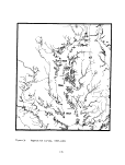 Table 22. Frequency of occurrence of vegetated samples, Vegetation Survey,
1967-1969
Percent transects vegetated
in
3
t/i ro
O •!-
r Ol •(->
Sampling station locations £ ro
ro d
i- •!-
-!-> S-
ro
"4- E
o
<o
S- S-
0) 01
E "i
3 0
ro
i *
>n.
s_
ro
E
ID
CL
O-
3
C£
O
HI
Q.
f-
o
QJ
cn
^
ro
o
Q.
(/>
•^
S-
+J
t/)
•r-
t/J
4J
fT3
r-
o
£_
OJ
Q.
•
D_
in
OJ
T3
ro
s=
ro
u
ro
OJ
•o
0
LjJ
3
ro
a.
ro
i —
r—
QJ
-C
u
«r"
C"
C
ro
M
ro
c
ro
r_>
•f—
S-
<D
ro
ro
•T—
^
Ol
c
U)
•r-
^~
r^
ro
>
E
3
4J
ro
o
a
l/V
E
3
i —
r-»
^
.C
a
o
^,
>.
2:
•
D. a.
a. a.
t/i (/)
ro t/>
i- ro
ro T-J
-c ro
0 Z
1967 Sampling
Pocomoke Sound
Big and Little Annemessex Rivers
Manokin River
Nanticoke and Wicomico Rivers
Fishing Bay
Smith Island
Honga River
Bloodsworth and Marsh Islands
1968 Sampling
Hooper and Taylor Islands
Little Choptank River
Choptank River
Eastern Bay
1969 Sampling
Kent and Love Points
Chester River
Howell and Swan Points
Sassafras River
Elk River
19 89 58
26 96 46 69
27 85 63
42 21 36
27 56 37 52
17 78 78
31 84 68 87
16 100 81 75
39 82 44 59
65 80 97 45 23
146 32 84 25 91 19 21
121 36 57 17 69 12 70
15 7 47 33
113 1 58 85 26 23 29 21 58 27 30
44 18 5 20 7 36 23 7 5
47 34 11 2 2
60 535
Maryland Wildlife Administration files 1977
b Locations correspond to area delineations of MBHRL Survey
136
image:
Table 22. Frequency of occurrence of vegetated samples, Vegetation Survey,
1967-1969
Percent transects vegetated
in
3
t/i ro
O •!-
r Ol •(->
Sampling station locations £ ro
ro d
i- •!-
-!-> S-
ro
"4- E
o
<o
S- S-
0) 01
E "i
3 0
ro
i *
>n.
s_
ro
E
ID
CL
O-
3
C£
O
HI
Q.
f-
o
QJ
cn
^
ro
o
Q.
(/>
•^
S-
+J
t/)
•r-
t/J
4J
fT3
r-
o
£_
OJ
Q.
•
D_
in
OJ
T3
ro
s=
ro
u
ro
OJ
•o
0
LjJ
3
ro
a.
ro
i —
r—
QJ
-C
u
«r"
C"
C
ro
M
ro
c
ro
r_>
•f—
S-
<D
ro
ro
•T—
^
Ol
c
U)
•r-
^~
r^
ro
>
E
3
4J
ro
o
a
l/V
E
3
i —
r-»
^
.C
a
o
^,
>.
2:
•
D. a.
a. a.
t/i (/)
ro t/>
i- ro
ro T-J
-c ro
0 Z
1967 Sampling
Pocomoke Sound
Big and Little Annemessex Rivers
Manokin River
Nanticoke and Wicomico Rivers
Fishing Bay
Smith Island
Honga River
Bloodsworth and Marsh Islands
1968 Sampling
Hooper and Taylor Islands
Little Choptank River
Choptank River
Eastern Bay
1969 Sampling
Kent and Love Points
Chester River
Howell and Swan Points
Sassafras River
Elk River
19 89 58
26 96 46 69
27 85 63
42 21 36
27 56 37 52
17 78 78
31 84 68 87
16 100 81 75
39 82 44 59
65 80 97 45 23
146 32 84 25 91 19 21
121 36 57 17 69 12 70
15 7 47 33
113 1 58 85 26 23 29 21 58 27 30
44 18 5 20 7 36 23 7 5
47 34 11 2 2
60 535
Maryland Wildlife Administration files 1977
b Locations correspond to area delineations of MBHRL Survey
136
image:
 E
^
c—
CL
O
"£
^-
E
-[_>
(O
(J
Cl
ro
., —
S-
tu
VI
,—
(O
fd
c:
rd
si
QJ
E
(/)
ro| (/I
0) c
-o 01
o -o
•- «
LjJ| £1
ro
<J
rc
•r-
'
c-
-r-
C
C
fd
r-*j
in
S-
-M
zs
rd
CL
c:
o
CD
en
0
E
rO
O
0-
in
^
ro
C
*\->
(J
QJ
CL
c
o
(U
CT
O
E
-4_>
O
^
4_1
rd
O
S-
OJ
CL
ro
Q.
Q.
3
E
+"*
s_
ro
E
ro
S-
<u
en
o
rO
.,_
i
t- </i
O C
0
<u +->
-O fO
E <->
3 t/1
^
O -C
•r- +J
4-> CL
rO CD
-t-> Q
OO
0)
S-
r_
£ £
01 >
0) 3
CD 1/1
•53" CO CO CM ^" CM i — 1
O O LO O O LO C\J
S- O O III O--HO OOl I 1 1 1
1—
<3" <— 1 O CO «^~ CO r- 1
m .-i en o •— i I-H o
111 III OO OOl OOl Oil
O i— i i — i i — 1< — iO OOO LO >— ( O
OOO III OOO OOO OOl Oil
LO CM i — 1 "•£> P-^
r--. LO ^-t ^r o
T-HOO III OOl III III III
co r^. i— i LO i — i i — i
O <-< <— I CM O O
OOl III OOl OOl ill ill
O"1 i-H CM CT* *d~ CTl "5J" O^ ^i" CO CO
LOOCM CMCO r-^r^.i — i ^3-1 — II-H
O t— I O OOl i— ii— iO OOO 111 III
fO CO i — I ^~ ^3" CTl ^J" ' — I r*^ LO
i— I OJ O COCO CTi T— i O COCM
«— I O O OOl OOO OOl III III
LO CO LO t— 1 i— t
o LO ro o O
000 liO iQl III ill III
cor^co CO^OLO rooiCTi roocn t— i CM LO c\i«cj-cM
CTlCOCO i — li — 1 i— ' CMQlCTi «^-^-CM LOCOCM kOLO«^l*
co *^ cTt co vo CTI ro <*o rji ro ^o CTI co <^3 CT^ co ^o cri
III III III III 111 III
s- >
QJ -r-
>> -a > >> a:
fd C ••- 4J
CQ <a o; c m s-
i — CU 13 OJ fd CU
c i/>s_ i- os- s- >
S-E — < O CUE OO 4-E -i- E
CUQJ jC -MQJ c~ rdQJ rV rjj
+->-(-> 4-Jin m-M -Mm m-M -M
</)in c>^ QJm c>) mm -^to
fO >•> QJ rd -^ >^ fiJ ro ro >i t— >^
LiJt/) i^CQ OCO i^CQ COLO LUC/)
4-> 0
Q--M
CD
"O "O
4-> -P
ro u
_C QJ
-l-> S-
S-
+J O
ro O
tn c
O QJ
-(->
rO +->
•4-> O
tn c:
M- QJ
o >
rd
S- -C
OJ
^H in
E -c
c: CL
QJ
>-) O
-O
-o •
-a o
>
-a c:
<d
OJ
cn =
c: r-t
JC =
4-> CM
Cur
QJ
t/> CO
Cnz •
O3 -1-i
S- -C S-
~o en o
Zi CL
OJ O QJ
y J_ ^_
fa -c:
s- -*-> in
M- ~D QJ
OS- S-
rd en
</> 3 o
Cn C S-
c: 3 CL
•i- O
+-> -a QJ
S- = 3
*fr O
OJ = _C
ra o
"O "
is en to
fa -c ul
QJ rd -O
> c
+J 0 r^
ra s- c:
13
E -a -o
Z3 QJ C
o en ro
c:
Erd QJ
S_ E
O ro
4- Cn CD
£Z
-a -r- M-
QJ -M 0
•r- S- +J
S- C
QJ QJ OJ
-a o E
C . -M
OJ fO S- S-
T3 ~D CU rO
ra C -t-> CL
s- 13 fa cu
en o 3 o
-a 3-0
cu o c:
en <u i —
•r- en c >>
in c: ro s-
in ro QJ ro
<c s- E s:
rO J3
137
image:
E
^
c—
CL
O
"£
^-
E
-[_>
(O
(J
Cl
ro
., —
S-
tu
VI
,—
(O
fd
c:
rd
si
QJ
E
(/)
ro| (/I
0) c
-o 01
o -o
•- «
LjJ| £1
ro
<J
rc
•r-
'
c-
-r-
C
C
fd
r-*j
in
S-
-M
zs
rd
CL
c:
o
CD
en
0
E
rO
O
0-
in
^
ro
C
*\->
(J
QJ
CL
c
o
(U
CT
O
E
-4_>
O
^
4_1
rd
O
S-
OJ
CL
ro
Q.
Q.
3
E
+"*
s_
ro
E
ro
S-
<u
en
o
rO
.,_
i
t- </i
O C
0
<u +->
-O fO
E <->
3 t/1
^
O -C
•r- +J
4-> CL
rO CD
-t-> Q
OO
0)
S-
r_
£ £
01 >
0) 3
CD 1/1
•53" CO CO CM ^" CM i — 1
O O LO O O LO C\J
S- O O III O--HO OOl I 1 1 1
1—
<3" <— 1 O CO «^~ CO r- 1
m .-i en o •— i I-H o
111 III OO OOl OOl Oil
O i— i i — i i — 1< — iO OOO LO >— ( O
OOO III OOO OOO OOl Oil
LO CM i — 1 "•£> P-^
r--. LO ^-t ^r o
T-HOO III OOl III III III
co r^. i— i LO i — i i — i
O <-< <— I CM O O
OOl III OOl OOl ill ill
O"1 i-H CM CT* *d~ CTl "5J" O^ ^i" CO CO
LOOCM CMCO r-^r^.i — i ^3-1 — II-H
O t— I O OOl i— ii— iO OOO 111 III
fO CO i — I ^~ ^3" CTl ^J" ' — I r*^ LO
i— I OJ O COCO CTi T— i O COCM
«— I O O OOl OOO OOl III III
LO CO LO t— 1 i— t
o LO ro o O
000 liO iQl III ill III
cor^co CO^OLO rooiCTi roocn t— i CM LO c\i«cj-cM
CTlCOCO i — li — 1 i— ' CMQlCTi «^-^-CM LOCOCM kOLO«^l*
co *^ cTt co vo CTI ro <*o rji ro ^o CTI co <^3 CT^ co ^o cri
III III III III 111 III
s- >
QJ -r-
>> -a > >> a:
fd C ••- 4J
CQ <a o; c m s-
i — CU 13 OJ fd CU
c i/>s_ i- os- s- >
S-E — < O CUE OO 4-E -i- E
CUQJ jC -MQJ c~ rdQJ rV rjj
+->-(-> 4-Jin m-M -Mm m-M -M
</)in c>^ QJm c>) mm -^to
fO >•> QJ rd -^ >^ fiJ ro ro >i t— >^
LiJt/) i^CQ OCO i^CQ COLO LUC/)
4-> 0
Q--M
CD
"O "O
4-> -P
ro u
_C QJ
-l-> S-
S-
+J O
ro O
tn c
O QJ
-(->
rO +->
•4-> O
tn c:
M- QJ
o >
rd
S- -C
OJ
^H in
E -c
c: CL
QJ
>-) O
-O
-o •
-a o
>
-a c:
<d
OJ
cn =
c: r-t
JC =
4-> CM
Cur
QJ
t/> CO
Cnz •
O3 -1-i
S- -C S-
~o en o
Zi CL
OJ O QJ
y J_ ^_
fa -c:
s- -*-> in
M- ~D QJ
OS- S-
rd en
</> 3 o
Cn C S-
c: 3 CL
•i- O
+-> -a QJ
S- = 3
*fr O
OJ = _C
ra o
"O "
is en to
fa -c ul
QJ rd -O
> c
+J 0 r^
ra s- c:
13
E -a -o
Z3 QJ C
o en ro
c:
Erd QJ
S_ E
O ro
4- Cn CD
£Z
-a -r- M-
QJ -M 0
•r- S- +J
S- C
QJ QJ OJ
-a o E
C . -M
OJ fO S- S-
T3 ~D CU rO
ra C -t-> CL
s- 13 fa cu
en o 3 o
-a 3-0
cu o c:
en <u i —
•r- en c >>
in c: ro s-
in ro QJ ro
<c s- E s:
rO J3
137
image:
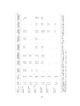 Migratory Bird and Habitat Research Laboratory (MBHRL) Survey, 1971 - present
In response to the need for a data base on SAV in the Chesapeake Bay, the
U.S. Fish and Wildlife Service Migratory Bird and Habitat Research Laboratory
(in Laurel, Maryland) established a summer sampling program of over 600 stations
within the Maryland Bay estuary. The objectives of the study were to measure
annual trends in abundance, composition and distribution of SAV; and to deter-
mine major environmental factors that might impact the vegetation (Kerwin et al.
1975; Munro 1976a[, 1976b). Sampling started the summer of 1971 and has con-
tinued to the present.
Based on percent acreage of Bay shoal waters (3.2 or less in depth at
mean low water), sample station locations were distributed among 26 river
system groups (see Figure 37) plus the Potomac River. The delineation of areas
based on river systems is not to be interpreted as drainage basins. Rather,
boundaries were drawn for ease of sampling and data presentation. Crews returned
to the individual established locations each year; however, an estimated error
factor of approximately 90 meters parallel to the contour was determined to be
acceptable in open areas such as the Susquehanna Flats (Munro, personal commun-
ication). At low tide it was occasionally necessary to relocate some stations
up to 180 m. Samples were run in triplicate with percent composition by species
based on a visual estimate.
In 1972, the MBHRL Survey included not only the Potomac River but also
portion of the Virginia section of the Chesapeake Bay. After 1972, these areas
were dropped from the survey until 1977 when sampling of the Potomac was resumed.
Haramis (1977) provided preliminary results of the Potomac stations which have
been included in this document. Available results for Tangier Island and
Pocomoke Sound (Virginia) have also been included for 1972. Preliminary results
for 1977 for stations located on the Eastern and Western Shores of the Maryland
Bay are limited to total vegetated stations by river area. Specific species
results will not be available until after June , 1978.
Table 24 shows annual percentage occurrence by river system and Table 25
depicts annual percentage occurrence by plant species. Based on six sampling
years, the following results have been noted (Kerwin et al. 1975; Munro 1976a^,
1976b):
• Significantly more vegetation was recorded in 1976 than
in 1975, though 1976 levels were still only one-half the recorded
level for 1971.
• Widgeongrass, horned-pondweed and redhead grass were the most fre-
guently recorded species over the six years.
• Sago pondweed, eel grass and wild celery continued to be recorded
infrequently.
• Concern had been expressed for the Choptank River after the 1975 survey.
However, vegetation in the Choptank showed a significant increase in
1976 over the extremely scarce occurrence in 1975.
138
image:
Migratory Bird and Habitat Research Laboratory (MBHRL) Survey, 1971 - present
In response to the need for a data base on SAV in the Chesapeake Bay, the
U.S. Fish and Wildlife Service Migratory Bird and Habitat Research Laboratory
(in Laurel, Maryland) established a summer sampling program of over 600 stations
within the Maryland Bay estuary. The objectives of the study were to measure
annual trends in abundance, composition and distribution of SAV; and to deter-
mine major environmental factors that might impact the vegetation (Kerwin et al.
1975; Munro 1976a[, 1976b). Sampling started the summer of 1971 and has con-
tinued to the present.
Based on percent acreage of Bay shoal waters (3.2 or less in depth at
mean low water), sample station locations were distributed among 26 river
system groups (see Figure 37) plus the Potomac River. The delineation of areas
based on river systems is not to be interpreted as drainage basins. Rather,
boundaries were drawn for ease of sampling and data presentation. Crews returned
to the individual established locations each year; however, an estimated error
factor of approximately 90 meters parallel to the contour was determined to be
acceptable in open areas such as the Susquehanna Flats (Munro, personal commun-
ication). At low tide it was occasionally necessary to relocate some stations
up to 180 m. Samples were run in triplicate with percent composition by species
based on a visual estimate.
In 1972, the MBHRL Survey included not only the Potomac River but also
portion of the Virginia section of the Chesapeake Bay. After 1972, these areas
were dropped from the survey until 1977 when sampling of the Potomac was resumed.
Haramis (1977) provided preliminary results of the Potomac stations which have
been included in this document. Available results for Tangier Island and
Pocomoke Sound (Virginia) have also been included for 1972. Preliminary results
for 1977 for stations located on the Eastern and Western Shores of the Maryland
Bay are limited to total vegetated stations by river area. Specific species
results will not be available until after June , 1978.
Table 24 shows annual percentage occurrence by river system and Table 25
depicts annual percentage occurrence by plant species. Based on six sampling
years, the following results have been noted (Kerwin et al. 1975; Munro 1976a^,
1976b):
• Significantly more vegetation was recorded in 1976 than
in 1975, though 1976 levels were still only one-half the recorded
level for 1971.
• Widgeongrass, horned-pondweed and redhead grass were the most fre-
guently recorded species over the six years.
• Sago pondweed, eel grass and wild celery continued to be recorded
infrequently.
• Concern had been expressed for the Choptank River after the 1975 survey.
However, vegetation in the Choptank showed a significant increase in
1976 over the extremely scarce occurrence in 1975.
138
image:
 NAUTICAL MILES
0 5 10 15 20 25
Figure37. River system sampling areas, Migratory Bird and Habitat Research
Laboratory Survey, 1971-present
139
image:
NAUTICAL MILES
0 5 10 15 20 25
Figure37. River system sampling areas, Migratory Bird and Habitat Research
Laboratory Survey, 1971-present
139
image:
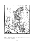 Table 24. Frequency of occurrence of vegetated samples and indicated change
by river systems, Migratory Bird and Habitat Research Laboratory Survey,
1971-19763
Area
code
1
2
3
4
5
6
7
8
9
10
11
12
13
14
15
16
17
18
19
20
21
22
23
24
25
26
River system
Elk & Bohemia
Rivers
Sassafras River
Howe 11 & Swan
Points
Eastern Bay
Choptank River
Little Choptank
River
James Island &
Honga River
Honga River
Bloodsworth Is.
Susquehanna
Flats
Fishing Bay
Nanticoke &
Wicomico Rivers
Manokin River
Patapsco River
Big & Little
Annemessex Rivers
Gunpowder & Bush
River Headwaters
Pocomoke Sound
(Maryland)
Magothy River
Severn River
Patuxent River
Back, Middle &
Gunpowder Rivers
Curtis & Cove
Points
South, West &
Rhode Rivers
Chester River
Love & Kent
Points
Smith Island
(Maryland)
Total
1971
% Veg.
6.67
30.00
16.67
34.04
35.00
21.05
44.12
50.00
37.50
44.44
8.00
0
40.00
0
70.00
11.11
18.18
33.33
40.00
2.00
13.64
0
0
61.11
0
64.71
28.53
1972
% Veg.
0
0
0
46.51
39.66
21.05
35.29
40.00
22.73
2.70
4.00
0
46.67
5.00
60.00
0
10.00
0
20.00
4.26
4.55
0
u
36.11
0
45.46
20.98
1973
% Veg.
0
0
0
34.04
19.30
0
2.94
13.33
10.87
0
0
0
13.33
4.76
30.00
0
4.76
16.67
26.67
0
4.55
0
0
26.47
0
25.00
10.49
1974
% Veg.
0
0
0
36.17
27.59
0
5.88
16.66
11.63
13.51
0
0
20.00
9.52
57.89
0
16.66
26.67
4.00
4.55
0
0
23.52
12.50
35.29
14.85
1975
X Veg.
0
0
0
21.74
1.72
0
5.88
10.35
6.98
11.11
0
0
7.14
33.33
15.00
-
-
0
9.09
0
0
25.00
0
22.22
8.70
197fi
% Veg.
0
0
0
42.22
41.07
15.79
8.82
17.24
2.22
8.57
0
0
6.67
9.52
30.00
0
9.09
16.67
46.15
2.04
4.55
0
12.50
26.71
0
35.29
14.97
1977b
* Veg.
0
0
0
28
25
5
3
3
4
11
0
0
20
14
30
11
10
25
20
2
9
0
0
38
0
24
12
Number
71
15
10
12
47
60
19
34
30
40
27
25
30
15
21
20
9
22
12
15
50
22
20
8
36
8
17
624
72
16
10
6
43
58
19
34
30
44
37
25
30
15
20
20
8
20
12
15
47
22
19
10
36
8
11
615
73
16
10
12
47
57
19
34
30
46
37
25
30
15
21
20
7
21
12
15
50
22
19
10
34
8
12
629
of stations
74
16
10
12
47
58
19
34
30
43
37
25
31
15
21
19
9
0
12
15
50
22
19
8
34
8
17
611
75
16
10
12
46
58
19
34
29
43
36
24
30
14
0
18
0
20
0
0
47
22
6
8
36
8
17
552
76
16
10
12
45
56
19
34
29
45
35
25
30
15
21
20
9
22
12
13
49
22
21
8
35
8
17
628
77
16
10
12
47
60
19
34
30
46
37
25
31
15
21
20
9
22
12
15
50
22
21
10
36
8
17
645
j> U.S. Fish and Wildlife Service Migratory Bird and Habitat Research Laboratory files 1977
° Preliminary results (Stotts, personal communication)
140
image:
Table 24. Frequency of occurrence of vegetated samples and indicated change
by river systems, Migratory Bird and Habitat Research Laboratory Survey,
1971-19763
Area
code
1
2
3
4
5
6
7
8
9
10
11
12
13
14
15
16
17
18
19
20
21
22
23
24
25
26
River system
Elk & Bohemia
Rivers
Sassafras River
Howe 11 & Swan
Points
Eastern Bay
Choptank River
Little Choptank
River
James Island &
Honga River
Honga River
Bloodsworth Is.
Susquehanna
Flats
Fishing Bay
Nanticoke &
Wicomico Rivers
Manokin River
Patapsco River
Big & Little
Annemessex Rivers
Gunpowder & Bush
River Headwaters
Pocomoke Sound
(Maryland)
Magothy River
Severn River
Patuxent River
Back, Middle &
Gunpowder Rivers
Curtis & Cove
Points
South, West &
Rhode Rivers
Chester River
Love & Kent
Points
Smith Island
(Maryland)
Total
1971
% Veg.
6.67
30.00
16.67
34.04
35.00
21.05
44.12
50.00
37.50
44.44
8.00
0
40.00
0
70.00
11.11
18.18
33.33
40.00
2.00
13.64
0
0
61.11
0
64.71
28.53
1972
% Veg.
0
0
0
46.51
39.66
21.05
35.29
40.00
22.73
2.70
4.00
0
46.67
5.00
60.00
0
10.00
0
20.00
4.26
4.55
0
u
36.11
0
45.46
20.98
1973
% Veg.
0
0
0
34.04
19.30
0
2.94
13.33
10.87
0
0
0
13.33
4.76
30.00
0
4.76
16.67
26.67
0
4.55
0
0
26.47
0
25.00
10.49
1974
% Veg.
0
0
0
36.17
27.59
0
5.88
16.66
11.63
13.51
0
0
20.00
9.52
57.89
0
16.66
26.67
4.00
4.55
0
0
23.52
12.50
35.29
14.85
1975
X Veg.
0
0
0
21.74
1.72
0
5.88
10.35
6.98
11.11
0
0
7.14
33.33
15.00
-
-
0
9.09
0
0
25.00
0
22.22
8.70
197fi
% Veg.
0
0
0
42.22
41.07
15.79
8.82
17.24
2.22
8.57
0
0
6.67
9.52
30.00
0
9.09
16.67
46.15
2.04
4.55
0
12.50
26.71
0
35.29
14.97
1977b
* Veg.
0
0
0
28
25
5
3
3
4
11
0
0
20
14
30
11
10
25
20
2
9
0
0
38
0
24
12
Number
71
15
10
12
47
60
19
34
30
40
27
25
30
15
21
20
9
22
12
15
50
22
20
8
36
8
17
624
72
16
10
6
43
58
19
34
30
44
37
25
30
15
20
20
8
20
12
15
47
22
19
10
36
8
11
615
73
16
10
12
47
57
19
34
30
46
37
25
30
15
21
20
7
21
12
15
50
22
19
10
34
8
12
629
of stations
74
16
10
12
47
58
19
34
30
43
37
25
31
15
21
19
9
0
12
15
50
22
19
8
34
8
17
611
75
16
10
12
46
58
19
34
29
43
36
24
30
14
0
18
0
20
0
0
47
22
6
8
36
8
17
552
76
16
10
12
45
56
19
34
29
45
35
25
30
15
21
20
9
22
12
13
49
22
21
8
35
8
17
628
77
16
10
12
47
60
19
34
30
46
37
25
31
15
21
20
9
22
12
15
50
22
21
10
36
8
17
645
j> U.S. Fish and Wildlife Service Migratory Bird and Habitat Research Laboratory files 1977
° Preliminary results (Stotts, personal communication)
140
image:
 rO
to
-a r-x
cu o->
n^ r j
\*J' n^
S_ 1
CU «— I
>-* p*x.
JD Cn
3 r-H
in
A
<*- >>
O 0)
in S-
OJ 3
•r- c/o
u
CU >5
Q. C
CO O
1 Jt
c: <o
•r- S-
o
CU -Q
rT» trt
w* «O
E —1
(C
-C .E
U O
s_
•O rO
CU CU
•P in
(O CU
0 CC
•5 -P
C ro
•r- -P
• r—
c-S
t— *V
ro :c
CU TD
U C
E ro
CU
i- TD
i_ S_
3 T-
0 OQ
O
0 >>
S-
M- 0
O 4->
to
>•> s-
u o>
E -r-
0) s:
3
o- «
cu to
S- -P
U_ C
rO
r—
• Q.
LO
CM O
• r—
CU 4->
r— ro
-Q 3
ro CT
t— ro
CO
O
E
CU
s-
£_
3
U
0
o
•P
E
CU
o
S-
cu
o_
to
r^
cr>
i-H
LO
r-*
CTi
i— i
«d-
r-^
cr>
t— i
co
r-^
o->
i— i
CM
f>*
CT>
i— 1
r— 1
r^
<Ti
I— 1
in
cu
•r—
U
0)
C3.
(/)
co
CM
0.
CM
r-H
CO
t
i-H
CO
<d-
CO
CO
i-H
r
CO r
•H CO CM
<4- o LO <d- I-H
•
• • *
O CO «— 1 i— I
i— 1
cr> r*.
o o o to o
V *
«* CO
r-H lO O» LO
CO O r
H r«. <3-
• * •
i— 1 O CH CM
to to <.
OO i-l r
• •
0 «* »-H
-1 O t-H
* • *
<* CM O O IO r-H
•51-
to
r
o
o
0>
»
o
CM
00
d
r^
«*
t
o
to
CT»
9
o
CM
r~>
*
o
•li-
t—i
••
I— 1
CO
<d-
,
o
I-H O1 tO CM CM tO ^f
*3-
*
CO
01
CM
•
LO
to
3
+J
to
•i —
i—
O
<4-
s-
<D
O.
C
0
+-)
O)
C7)
*
4->
O
O-
to o r
.
•^ a> ro
• * *
LO CM a> r>.
00 CM
^ vo
I— 1
•
o
CM
CM CO O !•*» CM f^
• •
i-H O
(
•1
4
(
r~
t
{
to
3 (
4-> I/I -i
ro 3 i-
C r— r-
•r- I — <
4-> -r- J
o to <
CU 3 -F
a. a. i
S
•l "l '
o_| o_| r«
• •
«d- o
i— 1 r-H
/)
_
«_
-)
n
3
a ro
5J E ro
•r- C
O -P •!-
•r- S-
S- rO
- (0 E
u e
= ro
J ro i-
- -r- CU
= Q- +*
r O- in
0 3 O
•J Oi M
•
CM
to
E
to
o
*l— •
i-
(U
£
ra
rO
• ^
S-
0)
E
to
f^
f—
rO
>•
t-H
•
1— I
LO
CO
»
co
£
3
4->
ra
o
•t—
Q.
to
E
3
p_
r—
>,
£
a.
o
T
>,
S
o
CO
»
o
to
CO
»
o
en
^J-
*
o
CM
co
,
o
to
«d-
•
1— I
«*
o
r
co
to
•r—
to
E
(U
-o
ro
E
ra
o
ro
cu
-o
o
LU
CM
co
r
o
*J-
LO
*
o
r>.
<=J-
f
t-H
LO
en
,
o
CO
CO
•
0
o
to
*
I— 1
in
• f—
in
E
cu
a.
3
r«
ro
"O
ra
3
O)
in
to
•o
ra
•z.
0
o
to
i-H
v
o
o
o
•*
to
n
0
E
3
to
cu
E
cu
•a
E
f.^
r_
>,
.E
Q.
o
•P
ra
s_
cu
o
to
1— 1
•
o
o
en
«3-
•
0
•sj-
to
o
co
CO
o
CM
co
*
o
•
Q.
Q.
in
rO
ro
.E
<_>
r^
^»
CT»
I-H
I/)
cu
•r-
(f-
>,
c
o
4_>
ra
o
J2
rO
_1
£1
o
s_
rO
cu
to
cu
o:
-P
ra
•P
JD
ra
rr~
T3
E
rO
•o
•r-
CQ
>,
c
o
•P
rO
en
•r—
rO
141
image:
rO
to
-a r-x
cu o->
n^ r j
\*J' n^
S_ 1
CU «— I
>-* p*x.
JD Cn
3 r-H
in
A
<*- >>
O 0)
in S-
OJ 3
•r- c/o
u
CU >5
Q. C
CO O
1 Jt
c: <o
•r- S-
o
CU -Q
rT» trt
w* «O
E —1
(C
-C .E
U O
s_
•O rO
CU CU
•P in
(O CU
0 CC
•5 -P
C ro
•r- -P
• r—
c-S
t— *V
ro :c
CU TD
U C
E ro
CU
i- TD
i_ S_
3 T-
0 OQ
O
0 >>
S-
M- 0
O 4->
to
>•> s-
u o>
E -r-
0) s:
3
o- «
cu to
S- -P
U_ C
rO
r—
• Q.
LO
CM O
• r—
CU 4->
r— ro
-Q 3
ro CT
t— ro
CO
O
E
CU
s-
£_
3
U
0
o
•P
E
CU
o
S-
cu
o_
to
r^
cr>
i-H
LO
r-*
CTi
i— i
«d-
r-^
cr>
t— i
co
r-^
o->
i— i
CM
f>*
CT>
i— 1
r— 1
r^
<Ti
I— 1
in
cu
•r—
U
0)
C3.
(/)
co
CM
0.
CM
r-H
CO
t
i-H
CO
<d-
CO
CO
i-H
r
CO r
•H CO CM
<4- o LO <d- I-H
•
• • *
O CO «— 1 i— I
i— 1
cr> r*.
o o o to o
V *
«* CO
r-H lO O» LO
CO O r
H r«. <3-
• * •
i— 1 O CH CM
to to <.
OO i-l r
• •
0 «* »-H
-1 O t-H
* • *
<* CM O O IO r-H
•51-
to
r
o
o
0>
»
o
CM
00
d
r^
«*
t
o
to
CT»
9
o
CM
r~>
*
o
•li-
t—i
••
I— 1
CO
<d-
,
o
I-H O1 tO CM CM tO ^f
*3-
*
CO
01
CM
•
LO
to
3
+J
to
•i —
i—
O
<4-
s-
<D
O.
C
0
+-)
O)
C7)
*
4->
O
O-
to o r
.
•^ a> ro
• * *
LO CM a> r>.
00 CM
^ vo
I— 1
•
o
CM
CM CO O !•*» CM f^
• •
i-H O
(
•1
4
(
r~
t
{
to
3 (
4-> I/I -i
ro 3 i-
C r— r-
•r- I — <
4-> -r- J
o to <
CU 3 -F
a. a. i
S
•l "l '
o_| o_| r«
• •
«d- o
i— 1 r-H
/)
_
«_
-)
n
3
a ro
5J E ro
•r- C
O -P •!-
•r- S-
S- rO
- (0 E
u e
= ro
J ro i-
- -r- CU
= Q- +*
r O- in
0 3 O
•J Oi M
•
CM
to
E
to
o
*l— •
i-
(U
£
ra
rO
• ^
S-
0)
E
to
f^
f—
rO
>•
t-H
•
1— I
LO
CO
»
co
£
3
4->
ra
o
•t—
Q.
to
E
3
p_
r—
>,
£
a.
o
T
>,
S
o
CO
»
o
to
CO
»
o
en
^J-
*
o
CM
co
,
o
to
«d-
•
1— I
«*
o
r
co
to
•r—
to
E
(U
-o
ro
E
ra
o
ro
cu
-o
o
LU
CM
co
r
o
*J-
LO
*
o
r>.
<=J-
f
t-H
LO
en
,
o
CO
CO
•
0
o
to
*
I— 1
in
• f—
in
E
cu
a.
3
r«
ro
"O
ra
3
O)
in
to
•o
ra
•z.
0
o
to
i-H
v
o
o
o
•*
to
n
0
E
3
to
cu
E
cu
•a
E
f.^
r_
>,
.E
Q.
o
•P
ra
s_
cu
o
to
1— 1
•
o
o
en
«3-
•
0
•sj-
to
o
co
CO
o
CM
co
*
o
•
Q.
Q.
in
rO
ro
.E
<_>
r^
^»
CT»
I-H
I/)
cu
•r-
(f-
>,
c
o
4_>
ra
o
J2
rO
_1
£1
o
s_
rO
cu
to
cu
o:
-P
ra
•P
JD
ra
rr~
T3
E
rO
•o
•r-
CQ
>,
c
o
•P
rO
en
•r—
rO
141
image:
 • Vegetation in the Bloodsworth Island area was at the lowest level
recorded during 1976.
• Salinities decreased significantly over the upper Bay averaging:
1971 15.441 ppt
1972 9.663 ppt
1973 10.371 ppt
1974 13.490 ppt
1975 10.956 ppt
1976 8.487 ppt
• Secchi disk readings were taken from 1972 through 1976 and showed a
small overall increase, indicating greater light penetration.
• Preliminary results from the 1977 survey indicate that the total
number vegetated stations decreased about 2 percent from the 1976
count.
MBHRL data related to individual species are presented in Chapter 1 in the
write-ups of the SAV species common to the Bay. The increase in light penetra-
tion documented by the MBHRL Survey is not consistent with the commonly held
notion that the Bay is becomming more turbid. Chapter 4 discusses the problems
and inconsistencies related to assessing turbidity.
Milfoil Survey, 1957-1977
In the late 1950s, in response to a growing concern and a need for infor-
mation concerning the infestation of Eurasian watermilfoil (Myriophyllum
spicatum) a network was formulated among various scientific organizations in
the Chesapeake Bay area. Over a 20-year period, the various organizations
involved in documenting the milfoil story included: Chesapeake Bay Laboratory
(University of Maryland), The Johns Hopkins University, U. S. Fish and Wildlife
Service Migratory Bird Habitat Research Laboratory, Maryland Wildlife Administra-
tion and the Maryland Department of Chesapeake Bay Affairs. Numerous adminis-
trative reports, lectures, progress reports and survey data are available through
these various organizations. For ease of presentation, these data have been
compiled in this report as a general Milfoil Survey.
Though the milfoil work w,as begun to study only Myriophyllum spicatum,
other species were documented. Myriophyllum infestations had such a negative
impact on indigenous SAV that it was necessary to study submerged aquatic species
in general. Though the years, many techniques were utilized for sampling.
However, for the purposes of this document, only general qualitative results
have been included. SAV documentation data from portions of the 20 years of
surveying have been compiled by the various organizations into several reports
that deal with observations by river system. These observations have been
142
image:
• Vegetation in the Bloodsworth Island area was at the lowest level
recorded during 1976.
• Salinities decreased significantly over the upper Bay averaging:
1971 15.441 ppt
1972 9.663 ppt
1973 10.371 ppt
1974 13.490 ppt
1975 10.956 ppt
1976 8.487 ppt
• Secchi disk readings were taken from 1972 through 1976 and showed a
small overall increase, indicating greater light penetration.
• Preliminary results from the 1977 survey indicate that the total
number vegetated stations decreased about 2 percent from the 1976
count.
MBHRL data related to individual species are presented in Chapter 1 in the
write-ups of the SAV species common to the Bay. The increase in light penetra-
tion documented by the MBHRL Survey is not consistent with the commonly held
notion that the Bay is becomming more turbid. Chapter 4 discusses the problems
and inconsistencies related to assessing turbidity.
Milfoil Survey, 1957-1977
In the late 1950s, in response to a growing concern and a need for infor-
mation concerning the infestation of Eurasian watermilfoil (Myriophyllum
spicatum) a network was formulated among various scientific organizations in
the Chesapeake Bay area. Over a 20-year period, the various organizations
involved in documenting the milfoil story included: Chesapeake Bay Laboratory
(University of Maryland), The Johns Hopkins University, U. S. Fish and Wildlife
Service Migratory Bird Habitat Research Laboratory, Maryland Wildlife Administra-
tion and the Maryland Department of Chesapeake Bay Affairs. Numerous adminis-
trative reports, lectures, progress reports and survey data are available through
these various organizations. For ease of presentation, these data have been
compiled in this report as a general Milfoil Survey.
Though the milfoil work w,as begun to study only Myriophyllum spicatum,
other species were documented. Myriophyllum infestations had such a negative
impact on indigenous SAV that it was necessary to study submerged aquatic species
in general. Though the years, many techniques were utilized for sampling.
However, for the purposes of this document, only general qualitative results
have been included. SAV documentation data from portions of the 20 years of
surveying have been compiled by the various organizations into several reports
that deal with observations by river system. These observations have been
142
image:
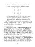 included in the conclusion section of this report and have been correlated with
the results of the other surveys.
South River, 1961
Philipp and Brown (1965) studied the distribution of SAV in two transi-
tional areas of the South River for 1961. One area was near the mouth of the
river in a small cove on the southeast side of Lime House Cove. The second
site was just north of the Route 50 bridge. Samples were taken at both sites
along transect lines and both plant species and bottom sediment were noted over
an eight year period.
Elodea canadensis dominated the northern site near the head of the river,
though relative abundance was considered sparse. Bottom sediment was found
to be muck/clay. The south site near the mouth of the river was dominated by
Potamogeton perfoliatus mixed with some Ruppia maritima and Myriophyllum
spicatum. This latter species and P_. perfoliatus dominated the deeper areas of
the cove (1.5 m maximum). Dense masses of Elodea nuttalli and £. perfoliatus
were observed at the surface. Sediments at this Icoation were mainly sand with
some sand/muck.
Philipp and Brown surveyed these two areas in the South River for a single
year in order to study species dominance, salinity, temperature and various
other water quality parameters. Their results have been included in order to
document SAV presence for 1961.
Rhode River, 1966-1973
Southwick and Pine (1975) surveyed SAV in the Rhode River starting with
preliminary observations in the early 1960s and continuing with extensive field
surveys from 1966 to 1973. Middle and Back Rivers were included for some of
the field surveys.
Surveys were made during the summer months, concentrated in June and July,
by traversing the shoreline to cover the area within the .6 to 1.2 m depth range
at mean low water. Results were plotted on maps for area! interpretation.
Table 26 depicts annual abundance for Rhode River in both hectares and indices
of abundance (see explanation at bottom of Table 20).
From observations and data over the survey's eight years, Myriophyllum and
P_. perfoliatus showed the most pronounced fluctuations in abundance. The latter
species plus Ruppia and P_. pectinatus disappeared entirely in 1970 though within
the next two years made at least a partial comeback. The eight year period
however, showed a general though erratic downward trend for all species.
Bay Bridge Tidal Pond, 1972-1975
From 1972 to 1975, James R. Goldsberry of the Maryland Wildlife Admini-
stration surveyed the submerged vegetation of the tidal pool that was created
at the east end of the Chesapeake Bay Bridge when the second bridge span was
constructed. Covering about 4 ha, the fill area provided an opportunity to
observe the natural succession of SAV into an essentially new area. Transects
143
image:
included in the conclusion section of this report and have been correlated with
the results of the other surveys.
South River, 1961
Philipp and Brown (1965) studied the distribution of SAV in two transi-
tional areas of the South River for 1961. One area was near the mouth of the
river in a small cove on the southeast side of Lime House Cove. The second
site was just north of the Route 50 bridge. Samples were taken at both sites
along transect lines and both plant species and bottom sediment were noted over
an eight year period.
Elodea canadensis dominated the northern site near the head of the river,
though relative abundance was considered sparse. Bottom sediment was found
to be muck/clay. The south site near the mouth of the river was dominated by
Potamogeton perfoliatus mixed with some Ruppia maritima and Myriophyllum
spicatum. This latter species and P_. perfoliatus dominated the deeper areas of
the cove (1.5 m maximum). Dense masses of Elodea nuttalli and £. perfoliatus
were observed at the surface. Sediments at this Icoation were mainly sand with
some sand/muck.
Philipp and Brown surveyed these two areas in the South River for a single
year in order to study species dominance, salinity, temperature and various
other water quality parameters. Their results have been included in order to
document SAV presence for 1961.
Rhode River, 1966-1973
Southwick and Pine (1975) surveyed SAV in the Rhode River starting with
preliminary observations in the early 1960s and continuing with extensive field
surveys from 1966 to 1973. Middle and Back Rivers were included for some of
the field surveys.
Surveys were made during the summer months, concentrated in June and July,
by traversing the shoreline to cover the area within the .6 to 1.2 m depth range
at mean low water. Results were plotted on maps for area! interpretation.
Table 26 depicts annual abundance for Rhode River in both hectares and indices
of abundance (see explanation at bottom of Table 20).
From observations and data over the survey's eight years, Myriophyllum and
P_. perfoliatus showed the most pronounced fluctuations in abundance. The latter
species plus Ruppia and P_. pectinatus disappeared entirely in 1970 though within
the next two years made at least a partial comeback. The eight year period
however, showed a general though erratic downward trend for all species.
Bay Bridge Tidal Pond, 1972-1975
From 1972 to 1975, James R. Goldsberry of the Maryland Wildlife Admini-
stration surveyed the submerged vegetation of the tidal pool that was created
at the east end of the Chesapeake Bay Bridge when the second bridge span was
constructed. Covering about 4 ha, the fill area provided an opportunity to
observe the natural succession of SAV into an essentially new area. Transects
143
image:
 c
0
1 %
CD
o>
(O
4-J
O
0-
1/5
3
1 ^
fO
C
4->
<J
CU
cx
<O
'r—
i —
"ou
s:
o
•r-
c
c
(O
M
00
£.
4->
I/)
3
r—-.
10
Q4
(O
•^™
a.
Q.
3
Qi
to
E
4->
• r—
S-
(O
C
o
4->
CU
CT
O
e
03
4->
o
a.
00
3
4->
to
•i —
I—
O
l+-
s-
cu
O.
e
B
-
>i
_c
a
o
•r-
S_
>,
£1
£
3
4->
<0
O
O.
t/>
J3
X
CU
T3
C
t—t
1/5
CU
(O
4->
O
CU
;n
J2
X
CD
-o
C
1 — 1
(/5
CD
s-
to
4->
O
CD
3:
J3
X
CD
•a
c
i — i
</5
CU
s_
to
4->
U
CD
^:
xi
X
CU
-a
c
i — i
00
CD
S-
<o
+->
u
CU
n:
JD
X
CD
T3
C
i — i
(/)
CD
S-
(O
4->
U
a>
n:
s-
(O
<U
>-
ovo^-oocyicx)co
• • • • • • •
CTl «* 1^. i-H VO <Tl CM
1—1
cncoi-H«j-ocMcooo
CM t-H CM O i-l CTl i-i
'd-cMor~.ooO'-i
• •••••••
or^cnr~-CMr-~cOLn
•—I <d" CO IO r-H
cocoir>^ncooor--LO
• •••••••
cooj^j-ojoojotn
r-H r-( CM
lOLDCOr^-OCMOOOO
• • • • • • •
lf> *t r-t If) OO <J3 i-H
CM i— 1 CM
ino*i-'sJ-o«-iojt-.
r^ CM co OJ 10 oo .-i
^-ir^Lnioooiooo
. • • • • •
<JO IO CO t— 1 CO »£>
O1 >£> <t
OJ r-i i— 1
t-lCMI^-CTlOOVOi-l
in oj «* i— i co CM
en co «=*•
io^j-voOoo^HU?Ln
• •••••••
Ot-H«*COOCMlOOJ
CO r-H
i — 1
r~-uDCOLf)cor~.cr>ur)
oooco^-ooco<-i
LD
yDi — cocno>— ICMCO
loioioioi — r~« r>« p~
CTl C71 CTl CTl O^ CTi CTl CTl
»-H 1 1 1— 1 1 1 1 1 ! 1 1 1 « 1
c
o
C •!-
0 4->
•r- (O
^ % 4->
(0 CU
4J a-
CU CU
O) C >
ai o
> ••- r—
4-> 03
4J (0 C
C 4-» O
x-^ <B CD -r-
O "O CD (/)
~— ' c cu as
i-H 3 > O
J3 O J=
4- (0 C O 4->
-CO 3
*— O14J £ CD O
u c: s E -c c i-
— ' T- O O 4-> -r- CD
CO 4-> S- U 2 4->
O O) O O r—
+ > S- S_ C 10
CD 4-> O D) O) C
^~ T3 C <4- X3 O
(O CU «3 C -i-
— > O i- "O i- O 5- I/)
voccuccuE<u<a
IO -r- 3-r- g T- O
W -O r— JD r— Or- O
E: a. to a. u a. o
Lf> II 3-r- -r- -r-
1^ XJ4-><4-4J<t-4-><+-
CTl •!— /Or— Or— O ' — O
i— 1 0} 3 3 3
«*- E </> E l/> E ">
* • • O CD CD CU
a> a> en s_ en j_ en s_
cuxsrtaciacio
•r- C CD -r- 4-> T- 4-> -r- 4->
Q.(O-O4->O4->O4->O
T3CcocD/acD(acu
•oci— is-.ci..c:s-.c
C 3
CO -Q
IO II II II II II II II
i^X
O 4- ••
•r- o«a;^o toco Oi-to
S
-C X CU
4-> CD S-
3 -O CD
o c .c
00 1-1 3
(O J3
144
image:
c
0
1 %
CD
o>
(O
4-J
O
0-
1/5
3
1 ^
fO
C
4->
<J
CU
cx
<O
'r—
i —
"ou
s:
o
•r-
c
c
(O
M
00
£.
4->
I/)
3
r—-.
10
Q4
(O
•^™
a.
Q.
3
Qi
to
E
4->
• r—
S-
(O
C
o
4->
CU
CT
O
e
03
4->
o
a.
00
3
4->
to
•i —
I—
O
l+-
s-
cu
O.
e
B
-
>i
_c
a
o
•r-
S_
>,
£1
£
3
4->
<0
O
O.
t/>
J3
X
CU
T3
C
t—t
1/5
CU
(O
4->
O
CU
;n
J2
X
CD
-o
C
1 — 1
(/5
CD
s-
to
4->
O
CD
3:
J3
X
CD
•a
c
i — i
</5
CU
s_
to
4->
U
CD
^:
xi
X
CU
-a
c
i — i
00
CD
S-
<o
+->
u
CU
n:
JD
X
CD
T3
C
i — i
(/)
CD
S-
(O
4->
U
a>
n:
s-
(O
<U
>-
ovo^-oocyicx)co
• • • • • • •
CTl «* 1^. i-H VO <Tl CM
1—1
cncoi-H«j-ocMcooo
CM t-H CM O i-l CTl i-i
'd-cMor~.ooO'-i
• •••••••
or^cnr~-CMr-~cOLn
•—I <d" CO IO r-H
cocoir>^ncooor--LO
• •••••••
cooj^j-ojoojotn
r-H r-( CM
lOLDCOr^-OCMOOOO
• • • • • • •
lf> *t r-t If) OO <J3 i-H
CM i— 1 CM
ino*i-'sJ-o«-iojt-.
r^ CM co OJ 10 oo .-i
^-ir^Lnioooiooo
. • • • • •
<JO IO CO t— 1 CO »£>
O1 >£> <t
OJ r-i i— 1
t-lCMI^-CTlOOVOi-l
in oj «* i— i co CM
en co «=*•
io^j-voOoo^HU?Ln
• •••••••
Ot-H«*COOCMlOOJ
CO r-H
i — 1
r~-uDCOLf)cor~.cr>ur)
oooco^-ooco<-i
LD
yDi — cocno>— ICMCO
loioioioi — r~« r>« p~
CTl C71 CTl CTl O^ CTi CTl CTl
»-H 1 1 1— 1 1 1 1 1 ! 1 1 1 « 1
c
o
C •!-
0 4->
•r- (O
^ % 4->
(0 CU
4J a-
CU CU
O) C >
ai o
> ••- r—
4-> 03
4J (0 C
C 4-» O
x-^ <B CD -r-
O "O CD (/)
~— ' c cu as
i-H 3 > O
J3 O J=
4- (0 C O 4->
-CO 3
*— O14J £ CD O
u c: s E -c c i-
— ' T- O O 4-> -r- CD
CO 4-> S- U 2 4->
O O) O O r—
+ > S- S_ C 10
CD 4-> O D) O) C
^~ T3 C <4- X3 O
(O CU «3 C -i-
— > O i- "O i- O 5- I/)
voccuccuE<u<a
IO -r- 3-r- g T- O
W -O r— JD r— Or- O
E: a. to a. u a. o
Lf> II 3-r- -r- -r-
1^ XJ4-><4-4J<t-4-><+-
CTl •!— /Or— Or— O ' — O
i— 1 0} 3 3 3
«*- E </> E l/> E ">
* • • O CD CD CU
a> a> en s_ en j_ en s_
cuxsrtaciacio
•r- C CD -r- 4-> T- 4-> -r- 4->
Q.(O-O4->O4->O4->O
T3CcocD/acD(acu
•oci— is-.ci..c:s-.c
C 3
CO -Q
IO II II II II II II II
i^X
O 4- ••
•r- o«a;^o toco Oi-to
S
-C X CU
4-> CD S-
3 -O CD
o c .c
00 1-1 3
(O J3
144
image:
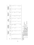 were run the length of the pond and samples were taken at depths from 15 to
100 cm. Bottom composition was found to be generally soft muck with occasional
sand or rock.
The first year, 1972, the pond yielded Ruppia maritime, Potamogeton
perfoliatus and Myriophyllum spicatum. The second year showed no new species
invaders4 By the third year, Potamogeton pusillus and El odea canadensis were
found along with the three species represented in 1972. By 1975, no new species
beyond the five already present were found.
In the summer of 1977, lush aquatic growth was again present and monitored
by the Maryland Wildlife Administration. Significant increases in El odea were
noted in July of 1977 along with extensive beds of P_. perfoliatus, scattered
Myriophyllum and a trace of P_. pectinatus (Jayne, personal communication). The
increase in the pond SAV that has been observed since 1972 compared to the docu-
mented decline in SAV in the Bay deserves further study. The lane that drains
into the pond is vegetated with grass and receives maintenance by state crews.
Therefore, it is microwatershed where there is little fertilizer input (Bridge
Authority personnel, personal communication) but where herbicides (dalopon and
amitol-t) have been sprayed for control of Phragmites around the pond. Also, it
does have high turbidity from carp populations which are capable of stirring up
bottom sediments (Stotts, personal communication).
Marshy Creek, 1975
The files of the Maryland Wildlife Administration contain a study of Marshy
Creek, south of Kent Narrows surveyed by James R. Goldsberry on July 7, 1975.
Documentation was made of the following species: Potamogeton perfoliatus,
Myriophyllum spicatum, Najas guadalupensis, Ruppia maritima, Chara sp.,
Zannichellia palustris and El odea canadensis.
Potamogeton perfoliatus and M_. spicatum were found primarily in the main-
stream of the creek. The inlets off the creek included some of these species
but were predominantly populated by Ruppia, Chara sp. and Najas. This study
has been included in order to further document species occurrence for the
Eastern Bay area.
Eastern Bay Survey, 1976
During the summer of 1976, George H. Fenwick, The Johns Hopkins University,
surveyed SAV in the Eastern Bay. The survey was part of a joint program initi-
ated by the Chesapeake Bay Foundation, The Johns Hopkins University waterfowl
research group and the Youth Conservation Corps.
The survey was based on a system of random transects located about 122
shoreline meters apart and extending about 55 m perpendicular to the shore.
Sampling stations were located at seven intervals along the 55 m transects. A
total of 2,192 stations were sampled in the Wye River and tributaries; Miles
River and tributaries; Kent Island; Rich Neck, including Claiborne Harbor; and
from Kent Narrows Bridge to Bennett Point. The survey spanned the time between
June 28 and August 27, 1976. The various parameters analyzed included: percent
occurrence, biomass, plant height, substrate and visual estimates of ground cover.
144 a
image:
were run the length of the pond and samples were taken at depths from 15 to
100 cm. Bottom composition was found to be generally soft muck with occasional
sand or rock.
The first year, 1972, the pond yielded Ruppia maritime, Potamogeton
perfoliatus and Myriophyllum spicatum. The second year showed no new species
invaders4 By the third year, Potamogeton pusillus and El odea canadensis were
found along with the three species represented in 1972. By 1975, no new species
beyond the five already present were found.
In the summer of 1977, lush aquatic growth was again present and monitored
by the Maryland Wildlife Administration. Significant increases in El odea were
noted in July of 1977 along with extensive beds of P_. perfoliatus, scattered
Myriophyllum and a trace of P_. pectinatus (Jayne, personal communication). The
increase in the pond SAV that has been observed since 1972 compared to the docu-
mented decline in SAV in the Bay deserves further study. The lane that drains
into the pond is vegetated with grass and receives maintenance by state crews.
Therefore, it is microwatershed where there is little fertilizer input (Bridge
Authority personnel, personal communication) but where herbicides (dalopon and
amitol-t) have been sprayed for control of Phragmites around the pond. Also, it
does have high turbidity from carp populations which are capable of stirring up
bottom sediments (Stotts, personal communication).
Marshy Creek, 1975
The files of the Maryland Wildlife Administration contain a study of Marshy
Creek, south of Kent Narrows surveyed by James R. Goldsberry on July 7, 1975.
Documentation was made of the following species: Potamogeton perfoliatus,
Myriophyllum spicatum, Najas guadalupensis, Ruppia maritima, Chara sp.,
Zannichellia palustris and El odea canadensis.
Potamogeton perfoliatus and M_. spicatum were found primarily in the main-
stream of the creek. The inlets off the creek included some of these species
but were predominantly populated by Ruppia, Chara sp. and Najas. This study
has been included in order to further document species occurrence for the
Eastern Bay area.
Eastern Bay Survey, 1976
During the summer of 1976, George H. Fenwick, The Johns Hopkins University,
surveyed SAV in the Eastern Bay. The survey was part of a joint program initi-
ated by the Chesapeake Bay Foundation, The Johns Hopkins University waterfowl
research group and the Youth Conservation Corps.
The survey was based on a system of random transects located about 122
shoreline meters apart and extending about 55 m perpendicular to the shore.
Sampling stations were located at seven intervals along the 55 m transects. A
total of 2,192 stations were sampled in the Wye River and tributaries; Miles
River and tributaries; Kent Island; Rich Neck, including Claiborne Harbor; and
from Kent Narrows Bridge to Bennett Point. The survey spanned the time between
June 28 and August 27, 1976. The various parameters analyzed included: percent
occurrence, biomass, plant height, substrate and visual estimates of ground cover.
144 a
image:
 All submerged vascular species of concern to this technical document were
found in the study area, with the exception of Chara spp. Results of the survey
include:
• 57.4 percent of the total number of stations were vegetated
• 48.3 percent of the total stations had 10 percent or more ground cover
• 24.2 percent of the total stations had abundant cover
• The Wye River was the mqst heavily vegetated area studied
* Ruppia maritima generally was considered to be dominant, occupying
52.7 percent of the total biomass
• £_. pectinatus was determined to be least common, with 4.0 percent of
the total biomass
' Zannichellia died back in mid-July
• P_. pectinatus was observed to die back in mid-August
• Ruppia increased in occurrence over the survey time span
This survey has been continued by the same joint effort though results are
not available at this time for 1977.
Chesapeake Bay Center for Environmental Studies (CBCES) - 1976-1977
CBCES (Smithsonian Institution) is presently studying the decline of sub-
merged aquatic vegetation in selected areas within the Chesapeake Bay (Correll
et al. 1976^, 1976b, 1977). The study is based on testing correlations between
plant die-offs, turbidity and herbicides. Station locations in the Rhode,
Choptank and Severn Rivers and the Poplar Island area are being sampled for SAV
populations, phytoplankton levels, turbidity of surface waters, suspended parti-
culates in surface waters, bottom sediment characteristics and herbicide levels.
Study objectives include analyzing the filtered water, suspended particulates
and bottom sediments for atrazine, alachlor, linuron and trifluralin. Specific
results of the field and bioassay work with Zannichellia palustris and herbicides
are discussed in Chapter 4.
Field surveys have documented SAV populations at established station »
locations throughout the four areas for 1976 and 1977. Results from the 1976
survey have been included in the conclusion section of this chapter.
Virginia Institute of Marine Science Surveys
Submerged aquatic vegetation in the waters of the Virginia portion of the
Chesapeake Bay is essentially the history of Zostera marina. Several other
species have been documented; however, the majority of the available information
on Virginia waters has resulted from the work of Robert Orth (VIMS) who has
145
image:
All submerged vascular species of concern to this technical document were
found in the study area, with the exception of Chara spp. Results of the survey
include:
• 57.4 percent of the total number of stations were vegetated
• 48.3 percent of the total stations had 10 percent or more ground cover
• 24.2 percent of the total stations had abundant cover
• The Wye River was the mqst heavily vegetated area studied
* Ruppia maritima generally was considered to be dominant, occupying
52.7 percent of the total biomass
• £_. pectinatus was determined to be least common, with 4.0 percent of
the total biomass
' Zannichellia died back in mid-July
• P_. pectinatus was observed to die back in mid-August
• Ruppia increased in occurrence over the survey time span
This survey has been continued by the same joint effort though results are
not available at this time for 1977.
Chesapeake Bay Center for Environmental Studies (CBCES) - 1976-1977
CBCES (Smithsonian Institution) is presently studying the decline of sub-
merged aquatic vegetation in selected areas within the Chesapeake Bay (Correll
et al. 1976^, 1976b, 1977). The study is based on testing correlations between
plant die-offs, turbidity and herbicides. Station locations in the Rhode,
Choptank and Severn Rivers and the Poplar Island area are being sampled for SAV
populations, phytoplankton levels, turbidity of surface waters, suspended parti-
culates in surface waters, bottom sediment characteristics and herbicide levels.
Study objectives include analyzing the filtered water, suspended particulates
and bottom sediments for atrazine, alachlor, linuron and trifluralin. Specific
results of the field and bioassay work with Zannichellia palustris and herbicides
are discussed in Chapter 4.
Field surveys have documented SAV populations at established station »
locations throughout the four areas for 1976 and 1977. Results from the 1976
survey have been included in the conclusion section of this chapter.
Virginia Institute of Marine Science Surveys
Submerged aquatic vegetation in the waters of the Virginia portion of the
Chesapeake Bay is essentially the history of Zostera marina. Several other
species have been documented; however, the majority of the available information
on Virginia waters has resulted from the work of Robert Orth (VIMS) who has
145
image:
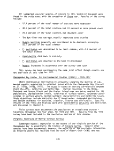 limited his research primarily to Zostera. The following section was written by
Orth and is submitted here as documentation of the history of Z^ marina in
Virginia.
Robert Orth. In Virginia, eel grass has been abundant on the Western Shore
in the York, Rappahannock and Piankatank Rivers, Mobjack Bay and its tributaries,
Back and Poquoson Rivers, Poquoson Flats area, Fleets Bay to the Potomac River
and on the Eastern Shore from Cape Charles to Tangier Sound. The first indica-
tions of a major decline came in the fall of 1973 (eelgrass had been abundant
that summer) though some local people reported eelgrass declined in the low
salinity regions of the estuary in 1972 after Tropical Storm Agnes. By 1974,
virtually all the eelgrass in the York, Rappahannock and Pinakatank rivers was
gone with significant declines in other areas (Table 27, Figure 38 and 39).
(Eastern Shore was not surveyed in 1974) (Orth and Gordon 1975; Orth 1976).
Table 27. Estimated total coverage of submerged aquatics for major
Virginia sections of the Chesapeake Bay, 1971 and 1974a
Major Areas
Back River
Plum Tree Island area
Poquoson Flats
Poquoson River
Crab Neck and Goodwin
1971
(ha)
144.9
868.2
233.8
66.1
306.7
1974
(ha)
211.9
466.5
59.9
111.7
219.4
Islands
York River 493.1 140.8
Mobjack Bay 1293.9 1592.6
New Point Comfort to 168.4 233.0
Pototo Neck
Gwynn's Island area 266.8 43.3
Piankatank River 306.9 21.2
Rappahannock River 699.6 3.6
Fleets Bay --- 197.6
Hampton area — 7.2
aOrth and Gordon, 1975
146
image:
limited his research primarily to Zostera. The following section was written by
Orth and is submitted here as documentation of the history of Z^ marina in
Virginia.
Robert Orth. In Virginia, eel grass has been abundant on the Western Shore
in the York, Rappahannock and Piankatank Rivers, Mobjack Bay and its tributaries,
Back and Poquoson Rivers, Poquoson Flats area, Fleets Bay to the Potomac River
and on the Eastern Shore from Cape Charles to Tangier Sound. The first indica-
tions of a major decline came in the fall of 1973 (eelgrass had been abundant
that summer) though some local people reported eelgrass declined in the low
salinity regions of the estuary in 1972 after Tropical Storm Agnes. By 1974,
virtually all the eelgrass in the York, Rappahannock and Pinakatank rivers was
gone with significant declines in other areas (Table 27, Figure 38 and 39).
(Eastern Shore was not surveyed in 1974) (Orth and Gordon 1975; Orth 1976).
Table 27. Estimated total coverage of submerged aquatics for major
Virginia sections of the Chesapeake Bay, 1971 and 1974a
Major Areas
Back River
Plum Tree Island area
Poquoson Flats
Poquoson River
Crab Neck and Goodwin
1971
(ha)
144.9
868.2
233.8
66.1
306.7
1974
(ha)
211.9
466.5
59.9
111.7
219.4
Islands
York River 493.1 140.8
Mobjack Bay 1293.9 1592.6
New Point Comfort to 168.4 233.0
Pototo Neck
Gwynn's Island area 266.8 43.3
Piankatank River 306.9 21.2
Rappahannock River 699.6 3.6
Fleets Bay --- 197.6
Hampton area — 7.2
aOrth and Gordon, 1975
146
image:
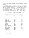 CTi
t—I
I
1^
oo
i.
OJ
s-
o
S-
O)
O)
o
c:
o
-Q
tl
CO
O
00
CO
OJ
CD
147
image:
CTi
t—I
I
1^
oo
i.
OJ
s-
o
S-
O)
O)
o
c:
o
-Q
tl
CO
O
00
CO
OJ
CD
147
image:
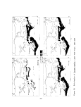 cu
13
o
o
CO
oo
148
image:
cu
13
o
o
CO
oo
148
image:
 •a
a;
4J
C
o
o
00
ro
a;
S-
149
image:
•a
a;
4J
C
o
o
00
ro
a;
S-
149
image:
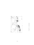 ARC* 29,1937 G,OUCESTER
\ POINT
Figure 39. Distribution of Zostera marina, Middle York River, 1937-1975
150
image:
ARC* 29,1937 G,OUCESTER
\ POINT
Figure 39. Distribution of Zostera marina, Middle York River, 1937-1975
150
image:
 Figure 39. (continued)
151
image:
Figure 39. (continued)
151
image:
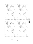 Recolonization by eelgrass occurred in some areas in 1974 via seedlings and
some vegetative growth but, in general, eelgrass density in these areas was very
low. In the late summer of 1975 eelgrass experienced a massive defoliation in
all areas of the lower Bay but by 1976, areas that had eelgrass in 1975 main-
tained some viable populations. There were some areas, for example in the
Mobjack Bay, that had a reduced density of eelgrass compared with 1975 (Orth,
personal observation). The regrowth during this period appeared to be from old
rhizome stock.
Eelgrass has undergone major fluctuations in the past in the Chesapeake Bay,
the most widely publicized decline being the one that occurred in the 1930s
(Burkholder and Doheny 1968; Cottam and Munro 1954). Eelgrass had reportedly
undergone changes in abundance in 1854 and 1889 to 1894 (Cottam 1934^, 1935b).
Following the 1930s decline when apparently most of the eelgrass died back in
the Bay, recovery of many eelgrass beds appeared to begin immediately. Two
areas in the York River, Mumfort Island and the mouth of the York River, where
the most intensive work on eelgrass beds in Virginia has occurred (Marsh 1970,
1973, 1976; Orth 1971, 1973, 1975^, 19755., 1976, 1977a., 1976bj Orth and Gordon
1975) were chosen for documentation of recovery since the 1930s. Aerial photo-
graphs obtained from the Department of Agriculture, National Oceanic and Atmos-
pheric Administration (NOAA) and VIMS showed a major increase between 1937 and
1953 with subsequent increases from 1953 to 1971. There appeared to be some
decline between 1960 and 1971 at Mumfort Island (see Figures 38 and 39). The
distribution of eelgrass in 1977 for these areas is very similar to that of 1974.
(Coverage for 1976 showed the distribution very similar to 1977).
It is interesting to note that the distribution of eelgrass in 1974 is
quite similar to the distribution of eelgrass in 1937. The disappearance of
eelgrass beginning in 1973 and past periods of decline in 1854, 1889 to 1894
and 1931 to 1932, suggest that there may be a natural cycle of eelgrass decline
every 40 years with local minor fluctuations superimposed on this major decline.
Walter I. Priest, III. The following documentation of SAV is the result
of field observations made in the Rappahannock and Piankatank Rivers and their
tidal tributaries in Middlesex County, Virginia. These observations were made
during an inventory of tidal wetlands performed by the Virginia Institute of
Marine Science. The shorelines of the above rivers and all of their tidal tri-
butaries were investigated by small boat during the months March to July, 1977.
The species encountered included: Zannichellia palustris, Zostera marina,
Ruppia maritima and Potamogeton (epihydrus ?).
Z_. palustris was most common in the tributaries of the Rappahannock River.
However, it was also encountered in several areas in the river proper plus the
Piankatank River and its tributaries. Rappahannock River salinities in these
areas vary from 7 to 13 ppt. Salinities in the individual creeks were not
measured. The habitats in which _Z. palustris produced the largest and most
prolific stands were the shallow areas at the heads of tidal creeks. The sub-
strate in these areas was usually loose silty mud. The stands of Z,. palustris
growing in the river proper were usually much sparser and not nearly as tall as
those growing in the headwater areas. The substrate in the river was most always
sand. The localities of occurrence are as follows and unless otherwise noted
152
image:
Recolonization by eelgrass occurred in some areas in 1974 via seedlings and
some vegetative growth but, in general, eelgrass density in these areas was very
low. In the late summer of 1975 eelgrass experienced a massive defoliation in
all areas of the lower Bay but by 1976, areas that had eelgrass in 1975 main-
tained some viable populations. There were some areas, for example in the
Mobjack Bay, that had a reduced density of eelgrass compared with 1975 (Orth,
personal observation). The regrowth during this period appeared to be from old
rhizome stock.
Eelgrass has undergone major fluctuations in the past in the Chesapeake Bay,
the most widely publicized decline being the one that occurred in the 1930s
(Burkholder and Doheny 1968; Cottam and Munro 1954). Eelgrass had reportedly
undergone changes in abundance in 1854 and 1889 to 1894 (Cottam 1934^, 1935b).
Following the 1930s decline when apparently most of the eelgrass died back in
the Bay, recovery of many eelgrass beds appeared to begin immediately. Two
areas in the York River, Mumfort Island and the mouth of the York River, where
the most intensive work on eelgrass beds in Virginia has occurred (Marsh 1970,
1973, 1976; Orth 1971, 1973, 1975^, 19755., 1976, 1977a., 1976bj Orth and Gordon
1975) were chosen for documentation of recovery since the 1930s. Aerial photo-
graphs obtained from the Department of Agriculture, National Oceanic and Atmos-
pheric Administration (NOAA) and VIMS showed a major increase between 1937 and
1953 with subsequent increases from 1953 to 1971. There appeared to be some
decline between 1960 and 1971 at Mumfort Island (see Figures 38 and 39). The
distribution of eelgrass in 1977 for these areas is very similar to that of 1974.
(Coverage for 1976 showed the distribution very similar to 1977).
It is interesting to note that the distribution of eelgrass in 1974 is
quite similar to the distribution of eelgrass in 1937. The disappearance of
eelgrass beginning in 1973 and past periods of decline in 1854, 1889 to 1894
and 1931 to 1932, suggest that there may be a natural cycle of eelgrass decline
every 40 years with local minor fluctuations superimposed on this major decline.
Walter I. Priest, III. The following documentation of SAV is the result
of field observations made in the Rappahannock and Piankatank Rivers and their
tidal tributaries in Middlesex County, Virginia. These observations were made
during an inventory of tidal wetlands performed by the Virginia Institute of
Marine Science. The shorelines of the above rivers and all of their tidal tri-
butaries were investigated by small boat during the months March to July, 1977.
The species encountered included: Zannichellia palustris, Zostera marina,
Ruppia maritima and Potamogeton (epihydrus ?).
Z_. palustris was most common in the tributaries of the Rappahannock River.
However, it was also encountered in several areas in the river proper plus the
Piankatank River and its tributaries. Rappahannock River salinities in these
areas vary from 7 to 13 ppt. Salinities in the individual creeks were not
measured. The habitats in which _Z. palustris produced the largest and most
prolific stands were the shallow areas at the heads of tidal creeks. The sub-
strate in these areas was usually loose silty mud. The stands of Z,. palustris
growing in the river proper were usually much sparser and not nearly as tall as
those growing in the headwater areas. The substrate in the river was most always
sand. The localities of occurrence are as follows and unless otherwise noted
152
image:
 the observed distribution was restricted to the heads of the creeks indicated
(see Figure 40);
Mason's Mill Swamp Meachims Creek, west of mouth in river
Mud Creek Greys Point, in river
Parrotts Creek Locklies Creek, near mouth
Weeks Creek Parrott Island, in river
Lagrange Creek Bush Park Creek
Urbanna Creek Piankatank River between Horse Pt. and
Whiting Creek Glebe Neck
My Lady's Swamp near head on Piankatank
River
The distribution of Ruppia maritima was apparently restricted to the lower
reaches of the Rappahannock and Piankatank Rivers. Several large stands were
observed near the mouth of Sturgeon Creek. It was also found growing in mono-
specific stands and mixed with Zostera marina on the offshore flats from the
mouth of Broad Creek around Stingray Point and up to the mouth of Jackson Creek
near the mouth of the Piankatank River. In addition, IR. maritima was found
growing in several tidal ponds along the Rappahannock River including one near
the mouth of Mill Creek and the two east of Duck Pond.
Zostera marina was observed in dense stands and in association with
R_. martima on the offshore sandflats from Broad Creek around Stingray Point to
O.ackson Creek. A broad floating-leaved pondweed tentatively indentified as
Potamogeton (epihydrus ?) was encountered at the heads of Mason's Mill Swamp and
LaGrange Creek near the upper limits of tidal influence in essentially fresh
water.
Herbarium Survey
Herbaria in the vicinity of the Chesapeake Bay have provided some informa-
tion as to historic occurrence of SAV. The data does not allow for interpre-
tation as to abundance or absence, but does indicate SAV presence as of the
specimen date. Documentation pertaining to the dominant submerged aquatic
species in the Bay was collected from the following herbaria:
University of Maryland, College Park, Maryland
Towson State University, Towson, Maryland
Smithsonian Institution, Washington, D.C.
Clyde Reed, (private collection)
Chesapeake Biological Laboratory, Solomons Island, Maryland
U. S. Fish and Wildlife Service Migratory Bird Habitat Research
Laboratory, Laurel, Maryland
The Smithsonian Institution herbarium contains the major holdings of
submerged aquatic species in the Chesapeake Bay area. Virginia herbaria were
not included in the survey due to time and distance problems.
Documentation of plant specimens has been organized along the format of
the river system groupings of the MBHRL sampling program. These observations
are included in the conclusion section at the end of this chapter.
153
image:
the observed distribution was restricted to the heads of the creeks indicated
(see Figure 40);
Mason's Mill Swamp Meachims Creek, west of mouth in river
Mud Creek Greys Point, in river
Parrotts Creek Locklies Creek, near mouth
Weeks Creek Parrott Island, in river
Lagrange Creek Bush Park Creek
Urbanna Creek Piankatank River between Horse Pt. and
Whiting Creek Glebe Neck
My Lady's Swamp near head on Piankatank
River
The distribution of Ruppia maritima was apparently restricted to the lower
reaches of the Rappahannock and Piankatank Rivers. Several large stands were
observed near the mouth of Sturgeon Creek. It was also found growing in mono-
specific stands and mixed with Zostera marina on the offshore flats from the
mouth of Broad Creek around Stingray Point and up to the mouth of Jackson Creek
near the mouth of the Piankatank River. In addition, IR. maritima was found
growing in several tidal ponds along the Rappahannock River including one near
the mouth of Mill Creek and the two east of Duck Pond.
Zostera marina was observed in dense stands and in association with
R_. martima on the offshore sandflats from Broad Creek around Stingray Point to
O.ackson Creek. A broad floating-leaved pondweed tentatively indentified as
Potamogeton (epihydrus ?) was encountered at the heads of Mason's Mill Swamp and
LaGrange Creek near the upper limits of tidal influence in essentially fresh
water.
Herbarium Survey
Herbaria in the vicinity of the Chesapeake Bay have provided some informa-
tion as to historic occurrence of SAV. The data does not allow for interpre-
tation as to abundance or absence, but does indicate SAV presence as of the
specimen date. Documentation pertaining to the dominant submerged aquatic
species in the Bay was collected from the following herbaria:
University of Maryland, College Park, Maryland
Towson State University, Towson, Maryland
Smithsonian Institution, Washington, D.C.
Clyde Reed, (private collection)
Chesapeake Biological Laboratory, Solomons Island, Maryland
U. S. Fish and Wildlife Service Migratory Bird Habitat Research
Laboratory, Laurel, Maryland
The Smithsonian Institution herbarium contains the major holdings of
submerged aquatic species in the Chesapeake Bay area. Virginia herbaria were
not included in the survey due to time and distance problems.
Documentation of plant specimens has been organized along the format of
the river system groupings of the MBHRL sampling program. These observations
are included in the conclusion section at the end of this chapter.
153
image:
 en
re
o
C_3
X
<u
(/)
01
T3
T3
I/)
re
O)
re
re
re
"a.
o
•P
re
cr
re
en
-Q
3
(/>
gp—
S-
_1 }
•T-^
IO
3
re
QL
re
i—
<u
Jd
o
• r—
c
c
re
M
VJ
3
s_
T3
>,
_^3
'o.
re
E
4J
tl
re
E
re
•r-
Q.
Q.
3
C£
O)
re
c
^
£••
re
s_
0)
-P
t/)
o
M
o
c
o
•p
3
_a
•r-
c^. s-
+j
to
£
O
-P
cu
0)
o
E
re
-p
o
Q-
•r-
Q
c3
.1 1
^r
gf
3
154
image:
en
re
o
C_3
X
<u
(/)
01
T3
T3
I/)
re
O)
re
re
re
"a.
o
•P
re
cr
re
en
-Q
3
(/>
gp—
S-
_1 }
•T-^
IO
3
re
QL
re
i—
<u
Jd
o
• r—
c
c
re
M
VJ
3
s_
T3
>,
_^3
'o.
re
E
4J
tl
re
E
re
•r-
Q.
Q.
3
C£
O)
re
c
^
£••
re
s_
0)
-P
t/)
o
M
o
c
o
•p
3
_a
•r-
c^. s-
+j
to
£
O
-P
cu
0)
o
E
re
-p
o
Q-
•r-
Q
c3
.1 1
^r
gf
3
154
image:
 Personal Communications
Just about everyone who has lived around the Chesapeake Bay in his/her
life has a remembrance of submerged aquatic vegetation. Often, the story is
of an unpleasant association: fouling of boat props, overgrowth of swimming
areas, noxious odors or decaying wind rows, etc. But many of the associations
have been pleasant: increased number of waterfowl for hunting, good fishing
and crabbing areas, etc. Thus, the relationship between humans and SAV has
been erratic and personal, a pleasure/pain existence.
Time does not permit the research necessary to extensively document this
relationship with first hand accounts. Also, such documentation would be of
questionable value to a scientific data base on SAV in the Chesapeake Bay since
memories are often faulty. However, in the course of the research effort for
this technical document several knowledgeable and aware individuals have been
contacted and interviewed. Summaries of these interviews are included in this
section.
Francis^ Uhler. MBHRL, January 10, 1977. Mr. Uhler speaks at length of
his 50-plus years of observations in the Chesapeake Bay area. His ready recall
of observations made in the late 1920s is as instantaneous as his 1977 recall.
Though most of his work has been along the Potomac River, his research has taken
him over most of the Maryland portion of the Bay at one time or another. Uhler
has amassed thousands of photographic slides taken since the 1930s. These
slides are presently being indexed and hopefully will be available sometime in
the future. The historic documentation that could be provided by Uhler's slide
collection would be invaluable to a general data base on SAV.
Some observations made by Uhler concerning his many years in the area
include:
• In Goose Bay (Port Tobacco River), Potomac River beds of Vallisneria
amerjicana were visible in 1976-1977 but greatly reduced from beds
present in the area in 1927. Marina dredging and algal blooms have
greatly changed the area. Port Tobacco River marinas have drastically
impacted the Vallisneria beds.
• In 1976, windrows of Vallisneria were seen along the banks of Popes
Creek and Persimmon Point, Potomac River.
• Luxuriant growths of Ruppia, IP. pectinatus and Vallisneria were seen
in the Potomac River prior to the 1931 drought. Vegetation returned
only in pockets.
• In the Blackwater Wildlife Refuge and Honga River area P_. pectinatus
and Zostera marina were seen prior to Agnes. Species of Chara common
to the area included C_. geobularis, C^. braunii, £. zeylam'ca and £.
hornamanii.
• Heavy beds of P_. pectinatus and Zostera were decimated by a bryozoan
4 to 5 years ago in Trippe Bay.
155
image:
Personal Communications
Just about everyone who has lived around the Chesapeake Bay in his/her
life has a remembrance of submerged aquatic vegetation. Often, the story is
of an unpleasant association: fouling of boat props, overgrowth of swimming
areas, noxious odors or decaying wind rows, etc. But many of the associations
have been pleasant: increased number of waterfowl for hunting, good fishing
and crabbing areas, etc. Thus, the relationship between humans and SAV has
been erratic and personal, a pleasure/pain existence.
Time does not permit the research necessary to extensively document this
relationship with first hand accounts. Also, such documentation would be of
questionable value to a scientific data base on SAV in the Chesapeake Bay since
memories are often faulty. However, in the course of the research effort for
this technical document several knowledgeable and aware individuals have been
contacted and interviewed. Summaries of these interviews are included in this
section.
Francis^ Uhler. MBHRL, January 10, 1977. Mr. Uhler speaks at length of
his 50-plus years of observations in the Chesapeake Bay area. His ready recall
of observations made in the late 1920s is as instantaneous as his 1977 recall.
Though most of his work has been along the Potomac River, his research has taken
him over most of the Maryland portion of the Bay at one time or another. Uhler
has amassed thousands of photographic slides taken since the 1930s. These
slides are presently being indexed and hopefully will be available sometime in
the future. The historic documentation that could be provided by Uhler's slide
collection would be invaluable to a general data base on SAV.
Some observations made by Uhler concerning his many years in the area
include:
• In Goose Bay (Port Tobacco River), Potomac River beds of Vallisneria
amerjicana were visible in 1976-1977 but greatly reduced from beds
present in the area in 1927. Marina dredging and algal blooms have
greatly changed the area. Port Tobacco River marinas have drastically
impacted the Vallisneria beds.
• In 1976, windrows of Vallisneria were seen along the banks of Popes
Creek and Persimmon Point, Potomac River.
• Luxuriant growths of Ruppia, IP. pectinatus and Vallisneria were seen
in the Potomac River prior to the 1931 drought. Vegetation returned
only in pockets.
• In the Blackwater Wildlife Refuge and Honga River area P_. pectinatus
and Zostera marina were seen prior to Agnes. Species of Chara common
to the area included C_. geobularis, C^. braunii, £. zeylam'ca and £.
hornamanii.
• Heavy beds of P_. pectinatus and Zostera were decimated by a bryozoan
4 to 5 years ago in Trippe Bay.
155
image:
 • In the Wye Narrows where P. pectinatus was abundant 5 years ago,
there is none.
• Canvasback stomach studies from the Nanticoke River presently show
only invertebrate material. The area is presently too turbid for
SAV.
• Gullet and stomach studies on Canvasbacks have shown that this
species has switched to an animal diet of Rangia, Macoma and Corbicula
Earl Abey, Waterman. May 27, 1977. Earl Abey has lived at Green Point for
over 50 years; his front porch is approximately 9 meters off the Choptank River.
"Up until 1970, the river in front of the house was like a wheat field, it was
so green," remembers Abey. Most of the Choptank was like that, with seasonal
SAV blooms protruding from the surface. In September, the vegetation normally
broke off at the rhizomes and floated in large masses to shore.
Dr. Eugene Cronin went out on the Choptank with Abey in 1944. At this
time Abey remembers extensive vegetation stands. Up until 1970, he used to cut
channels for his boats to get out, but today he goes out to the docks and sees
only a sprig or two.
Compared to other areas of the Choptank, Green Point is secluded and
therefore protected. During the summer an algal and scum layer would stagnate
above the rooted aquatics. Abey feels that with the decline in vegetation, he
receives more wave activity near his docks.
Abey attributes the vegetation decline to herbicides runoff from farmland.
He remembers an example of herbicides affecting vegetation control some 20 years
ago when someone put a gallon of herbicide ina pond near his house. Vegetation
has never returned.
Even though rooted aquatics have declined, Abey finds that crabs are still
abundant in the deeper waters. However, he does not know how the vegetation
loss will affect the seafood population in the long run.
CONCLUSIONS
In order to synthesize the diverse data sources (surveys, specimens,
personal communications, etc.) into a more logical and simplistic structure the
river system delineations utilized in the MBHRL study will serve as an organi-
zational format. This areal partitioning of the Maryland portion of the
Chesapeake Bay has been previously shown in Figure 37. Data for the Potomac
River includes both the Maryland and Virginia sides of the River. Virginia
vegetation documentation is listed by major river systems. Table 28 provides a
source key for following historic documentation tables.
Area 1. Elk and Bohemia Rivers
The first documentation of SAV in the Elk and Bohemia Rivers dates back
to 1955 herbarium specimens of P_. perfoliatus, Vallisneria and El odea
156
image:
• In the Wye Narrows where P. pectinatus was abundant 5 years ago,
there is none.
• Canvasback stomach studies from the Nanticoke River presently show
only invertebrate material. The area is presently too turbid for
SAV.
• Gullet and stomach studies on Canvasbacks have shown that this
species has switched to an animal diet of Rangia, Macoma and Corbicula
Earl Abey, Waterman. May 27, 1977. Earl Abey has lived at Green Point for
over 50 years; his front porch is approximately 9 meters off the Choptank River.
"Up until 1970, the river in front of the house was like a wheat field, it was
so green," remembers Abey. Most of the Choptank was like that, with seasonal
SAV blooms protruding from the surface. In September, the vegetation normally
broke off at the rhizomes and floated in large masses to shore.
Dr. Eugene Cronin went out on the Choptank with Abey in 1944. At this
time Abey remembers extensive vegetation stands. Up until 1970, he used to cut
channels for his boats to get out, but today he goes out to the docks and sees
only a sprig or two.
Compared to other areas of the Choptank, Green Point is secluded and
therefore protected. During the summer an algal and scum layer would stagnate
above the rooted aquatics. Abey feels that with the decline in vegetation, he
receives more wave activity near his docks.
Abey attributes the vegetation decline to herbicides runoff from farmland.
He remembers an example of herbicides affecting vegetation control some 20 years
ago when someone put a gallon of herbicide ina pond near his house. Vegetation
has never returned.
Even though rooted aquatics have declined, Abey finds that crabs are still
abundant in the deeper waters. However, he does not know how the vegetation
loss will affect the seafood population in the long run.
CONCLUSIONS
In order to synthesize the diverse data sources (surveys, specimens,
personal communications, etc.) into a more logical and simplistic structure the
river system delineations utilized in the MBHRL study will serve as an organi-
zational format. This areal partitioning of the Maryland portion of the
Chesapeake Bay has been previously shown in Figure 37. Data for the Potomac
River includes both the Maryland and Virginia sides of the River. Virginia
vegetation documentation is listed by major river systems. Table 28 provides a
source key for following historic documentation tables.
Area 1. Elk and Bohemia Rivers
The first documentation of SAV in the Elk and Bohemia Rivers dates back
to 1955 herbarium specimens of P_. perfoliatus, Vallisneria and El odea
156
image:
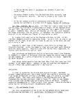 Table 28. Historic documentation key
(A) Anderson et al. (1967)
(B) Benthic Survey
(CB) Chesapeake Bay Center for Environmental Studies
(E) Elser (1969)
(EC) Ecological Analysts, Inc. (Pine, personal communication)
(F) Eastern Bay Survey (Fenwick, unpublished)
(G) Marshy Creek Survey
(H) Herbarium specimen
(HP) Horn Point Environmental Laboratories
(M) Milfoil Survey
(MB) MBHRL Survey (Kerwin et al. 1975; Munro 1976a_, 1976bj
(0) Orth, VIMS
(P) Pine, personal observation
(P&P) South River Survey (Philipp and Brown 1965)
(RS) Stewart (1962)
(S) Susquehanna Flats Survey (Bayley et al. in press)
(SO) Southwick (1967-1969)
(S&P) Rhode River Survey (Southwick and Pine 1975)
(U) Uhler, personal observation
(V) Vegetation Survey
(VS) Stotts, personal communication
(WP) Priest, VIMS
157
image:
Table 28. Historic documentation key
(A) Anderson et al. (1967)
(B) Benthic Survey
(CB) Chesapeake Bay Center for Environmental Studies
(E) Elser (1969)
(EC) Ecological Analysts, Inc. (Pine, personal communication)
(F) Eastern Bay Survey (Fenwick, unpublished)
(G) Marshy Creek Survey
(H) Herbarium specimen
(HP) Horn Point Environmental Laboratories
(M) Milfoil Survey
(MB) MBHRL Survey (Kerwin et al. 1975; Munro 1976a_, 1976bj
(0) Orth, VIMS
(P) Pine, personal observation
(P&P) South River Survey (Philipp and Brown 1965)
(RS) Stewart (1962)
(S) Susquehanna Flats Survey (Bayley et al. in press)
(SO) Southwick (1967-1969)
(S&P) Rhode River Survey (Southwick and Pine 1975)
(U) Uhler, personal observation
(V) Vegetation Survey
(VS) Stotts, personal communication
(WP) Priest, VIMS
157
image:
 (see Table 29). Documentation through the 1960s and until 1971 indicates the con-
tinued presence of five species. However, since 1971, no plants have been
observed by the MBHRL Survey. P_. perfoliatus has not been documented since
1962 and El odea since 1969. Milfoil Survey personnel (1970-1971) found SAV
growth to be diversified but sparse and limited to indentations in the lower
part of the Elk River and the upper reaches of Veazey Cove, Bohemia River.
Channel deepening in the Elk River and C & D Canal resulted in a heavy silt
load that was readily apparent in August of 1969. No vegetation was observed
in the turbid waters of Cabin John Creek below the Bohemia River.
Table 29. Historic documentation of SAV by decades, Elk and Bohemia
Rivers, Maryland (Area 1)
Species
Potamogeton
perfonatus
CeratophyTlum
demersum
Myriophyllum
spicatum
Zannichellia
gal ustri s
VaTlisneria
americana
El odea
canadensis
Chara spp.
1950
1960
1970
1955(H) 1962(H)
1955(H)
1955(H)
1961,1969(M)
1961,1967-1969(M)
1963,1968(H)
1969(V)
1961,1969(M)
1969(V)
1961,1969(M)
1961,1969(M)
1968(H)
1969(V)
1970-197KM)
1970-1971(M)
1970-1971(M)
1970-1971(M)
1971(MB)
1970-1971(M)
Area 2. Sassafras River
Herbarium specimens date back to 1947 and 1952 for the Sassafras River
(see Table 30). During the 1960s, survey teams documented a total of seven
species. Elser (1969) reported extensive stands of Myriophyllum, Ceratophyllurn,
Vallisneria, P_. crispus, El odea and Najas in the Sassafras River and its tribu-
taries in the early 1960s. By 1966, vegetation seemed to be limited to the
tributary mouths and the lower central portions. Beds have previously been
seen in intertidal areas plus the upper parts of the tributaries and from the
shore out 6 to 15 m. In 1967, Elser observed what he termed the "Rhode River
Evanescence" when only a few sparse SAV beds were found. Vallisneria and
Ceratophyllum displayed a growth resurgence after the decline in Myriophyllum;
however, abundance levels never seemed to reach prior levels.
158
image:
(see Table 29). Documentation through the 1960s and until 1971 indicates the con-
tinued presence of five species. However, since 1971, no plants have been
observed by the MBHRL Survey. P_. perfoliatus has not been documented since
1962 and El odea since 1969. Milfoil Survey personnel (1970-1971) found SAV
growth to be diversified but sparse and limited to indentations in the lower
part of the Elk River and the upper reaches of Veazey Cove, Bohemia River.
Channel deepening in the Elk River and C & D Canal resulted in a heavy silt
load that was readily apparent in August of 1969. No vegetation was observed
in the turbid waters of Cabin John Creek below the Bohemia River.
Table 29. Historic documentation of SAV by decades, Elk and Bohemia
Rivers, Maryland (Area 1)
Species
Potamogeton
perfonatus
CeratophyTlum
demersum
Myriophyllum
spicatum
Zannichellia
gal ustri s
VaTlisneria
americana
El odea
canadensis
Chara spp.
1950
1960
1970
1955(H) 1962(H)
1955(H)
1955(H)
1961,1969(M)
1961,1967-1969(M)
1963,1968(H)
1969(V)
1961,1969(M)
1969(V)
1961,1969(M)
1961,1969(M)
1968(H)
1969(V)
1970-197KM)
1970-1971(M)
1970-1971(M)
1970-1971(M)
1971(MB)
1970-1971(M)
Area 2. Sassafras River
Herbarium specimens date back to 1947 and 1952 for the Sassafras River
(see Table 30). During the 1960s, survey teams documented a total of seven
species. Elser (1969) reported extensive stands of Myriophyllum, Ceratophyllurn,
Vallisneria, P_. crispus, El odea and Najas in the Sassafras River and its tribu-
taries in the early 1960s. By 1966, vegetation seemed to be limited to the
tributary mouths and the lower central portions. Beds have previously been
seen in intertidal areas plus the upper parts of the tributaries and from the
shore out 6 to 15 m. In 1967, Elser observed what he termed the "Rhode River
Evanescence" when only a few sparse SAV beds were found. Vallisneria and
Ceratophyllum displayed a growth resurgence after the decline in Myriophyllum;
however, abundance levels never seemed to reach prior levels.
158
image:
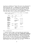 Table 30. Historic documentation of SAV by decades, Sassafras River,
Maryland (Area 2)
Species
1940
1950
1960
1970
Potamogeton 1947(H) 1952(H) 1968-1969(M)
perfollatus
Myriophyllum
spicatum
Vallisneria
americana
Elodea
canadensis
Chara spp.
Ceratophyllum
demersum
1960s(E)
1961(M)
1965(H)
1969(V)
1952(H) 1960s(E)
1961,1969(M)
1969(V)
1952(H) 1961,1969(M)
1952(H) 1960s(E)
1961, 1969(M)
1969(V)
1969(V)
1960s(E)
1961,1968-1969(M)
1970-1971(M)
1971-1974(MB)
1970-1971(M)
1971(MB)
Experimental herbicidal control measures were used in Revuques Pond and
Shellcross embayments in 1968 for Myriophyllum control. In Revuques Pond, the
experiment was considered to be 95 percent effective and resulted in dominant
growth of Najas in 1969. In the Shellcross embayment, Myriophyllum control
resulted in the dominance of Vallisneria in 1969.
The 1970-1971 Milfoil Survey found Myriophyllum to be dominant in several
embayments along the southern shore of the Sassafras River. Some resurge in
growth of Vallisneria was noted in Shell cross embayment and along the northern
shore. Nothing but sparse vegetation had been observed in Cox, Freeman Island,
Woodland and Dyer Creeks since 1966. In 1967, the water in these creeks was
observed to contain a heavy silt load and plankton blooms. In Turner, Money
and Foreman Creeks, the water was also clouded by a heavy silt load and only
scattered SAV beds were noted.
Area 3. Howell and Swan Points
t
A Ruppia herbarium specimen from 1907 is the first documented SAV species
listed for Howell and Swan Points (see Table 31). By the 1960s, three survey
terms had documented nine aquatic species. Milfoil Survey personnel surveyed
Still pond Creek and found sparse growths of Vallisneria in 1970, substantial
Vallisneria in 1971 and a seeming reinvasion of Myriophyllum during 1970 and
1971. The MBHRL Survey found good growths of Vanisneria and traces of
Myriophyl1 urn in Stillpond Creek in 1971. There has been no documentation of any
vegetation in Stillpond Creek or in the rest of Area 3 since 1971 with the ex-
ception of Stotts who noted dense beds of what may have been milfoil in the
lower portion of the creek. These beds were noted on November 14, 1977, during
an aerial survey of Canada geese.
159
image:
Table 30. Historic documentation of SAV by decades, Sassafras River,
Maryland (Area 2)
Species
1940
1950
1960
1970
Potamogeton 1947(H) 1952(H) 1968-1969(M)
perfollatus
Myriophyllum
spicatum
Vallisneria
americana
Elodea
canadensis
Chara spp.
Ceratophyllum
demersum
1960s(E)
1961(M)
1965(H)
1969(V)
1952(H) 1960s(E)
1961,1969(M)
1969(V)
1952(H) 1961,1969(M)
1952(H) 1960s(E)
1961, 1969(M)
1969(V)
1969(V)
1960s(E)
1961,1968-1969(M)
1970-1971(M)
1971-1974(MB)
1970-1971(M)
1971(MB)
Experimental herbicidal control measures were used in Revuques Pond and
Shellcross embayments in 1968 for Myriophyllum control. In Revuques Pond, the
experiment was considered to be 95 percent effective and resulted in dominant
growth of Najas in 1969. In the Shellcross embayment, Myriophyllum control
resulted in the dominance of Vallisneria in 1969.
The 1970-1971 Milfoil Survey found Myriophyllum to be dominant in several
embayments along the southern shore of the Sassafras River. Some resurge in
growth of Vallisneria was noted in Shell cross embayment and along the northern
shore. Nothing but sparse vegetation had been observed in Cox, Freeman Island,
Woodland and Dyer Creeks since 1966. In 1967, the water in these creeks was
observed to contain a heavy silt load and plankton blooms. In Turner, Money
and Foreman Creeks, the water was also clouded by a heavy silt load and only
scattered SAV beds were noted.
Area 3. Howell and Swan Points
t
A Ruppia herbarium specimen from 1907 is the first documented SAV species
listed for Howell and Swan Points (see Table 31). By the 1960s, three survey
terms had documented nine aquatic species. Milfoil Survey personnel surveyed
Still pond Creek and found sparse growths of Vallisneria in 1970, substantial
Vallisneria in 1971 and a seeming reinvasion of Myriophyllum during 1970 and
1971. The MBHRL Survey found good growths of Vanisneria and traces of
Myriophyl1 urn in Stillpond Creek in 1971. There has been no documentation of any
vegetation in Stillpond Creek or in the rest of Area 3 since 1971 with the ex-
ception of Stotts who noted dense beds of what may have been milfoil in the
lower portion of the creek. These beds were noted on November 14, 1977, during
an aerial survey of Canada geese.
159
image:
 Table 31. Historic documentation of SAV by decades, Howell and Swan
Points, Maryland (Area 3)
Species
1900
1940
1960
1970
Potamogeton
perfoliatus
Ruppia 1907(H)
maritima
Myrlophyllum
spicatum
P. pectinatus
Vallisneria
americana
ETodea
canadensis
Najas spp.
Chara spp.
Ceratophyl 1 urn
demersum
1961(M)
1965-1969(M)
1969(V)
1965,1969(M)
1969(V)
1961(B)(M)
1965,1969(M)
1969(V)
1969(V)
1947(H) 1961 (B)(M)
1965,1969(M)
1969(V)
1965(M)
1969(V)
1947(H) 1961(B)
1969(V)
1969(V)
1969(M)
1971(MB)
1970-1971(M)
1971(MB)
1970-1971(M)
Area 4. Eastern Bay
Percentages figures from the MBHRL Survey showing number of stations with
vegetation indicate a fairly steady total population over the six years (see
Table 24). Ruppia remained dominant and a strong resurge in growth seemed to
have taken place between the 1975 and 1976 summer samplings. Trace amounts of
£. perfoliatus, Myriophyllum and Zannichellia were found in 1976 and P_. pectinatus
and El odea were documented in occasional patches.
Frank Pine, then a graduate student at The Johns Hopkins University, sur-
veyed the Miles River from 1971 through 1974 (Pine, personal communication).
Ruppia, P_. pectinatus, P_. perfoliatus and Zannichellia were documented for all
four years around Claiborne, Rich Neck and Long Point. All species occurred
throughout the four years though a definite decline in abundance was noted by
1974.
Pine surveyed Parsons Island in Eastern Bay in May, 1974, and found
IP. pectinatus to be extremely abundant. The beds seemed to be at absolute
maximum production with some plants up to 1.8 m in length. By 1975, vegetation
appeared to be considerably less. In August and September, 1974, Pine surveyed
the Horse Head Farm area. Populations were mixed: _P. perfoliatus was the most
common throughout the shorelines; Ruppia was common to occasional; and Elodea
was found occasionally. Myriophyllum was determined to be locally abundant to
occasional on the north side of the island. Zannichellia was not seen, probably
160
image:
Table 31. Historic documentation of SAV by decades, Howell and Swan
Points, Maryland (Area 3)
Species
1900
1940
1960
1970
Potamogeton
perfoliatus
Ruppia 1907(H)
maritima
Myrlophyllum
spicatum
P. pectinatus
Vallisneria
americana
ETodea
canadensis
Najas spp.
Chara spp.
Ceratophyl 1 urn
demersum
1961(M)
1965-1969(M)
1969(V)
1965,1969(M)
1969(V)
1961(B)(M)
1965,1969(M)
1969(V)
1969(V)
1947(H) 1961 (B)(M)
1965,1969(M)
1969(V)
1965(M)
1969(V)
1947(H) 1961(B)
1969(V)
1969(V)
1969(M)
1971(MB)
1970-1971(M)
1971(MB)
1970-1971(M)
Area 4. Eastern Bay
Percentages figures from the MBHRL Survey showing number of stations with
vegetation indicate a fairly steady total population over the six years (see
Table 24). Ruppia remained dominant and a strong resurge in growth seemed to
have taken place between the 1975 and 1976 summer samplings. Trace amounts of
£. perfoliatus, Myriophyllum and Zannichellia were found in 1976 and P_. pectinatus
and El odea were documented in occasional patches.
Frank Pine, then a graduate student at The Johns Hopkins University, sur-
veyed the Miles River from 1971 through 1974 (Pine, personal communication).
Ruppia, P_. pectinatus, P_. perfoliatus and Zannichellia were documented for all
four years around Claiborne, Rich Neck and Long Point. All species occurred
throughout the four years though a definite decline in abundance was noted by
1974.
Pine surveyed Parsons Island in Eastern Bay in May, 1974, and found
IP. pectinatus to be extremely abundant. The beds seemed to be at absolute
maximum production with some plants up to 1.8 m in length. By 1975, vegetation
appeared to be considerably less. In August and September, 1974, Pine surveyed
the Horse Head Farm area. Populations were mixed: _P. perfoliatus was the most
common throughout the shorelines; Ruppia was common to occasional; and Elodea
was found occasionally. Myriophyllum was determined to be locally abundant to
occasional on the north side of the island. Zannichellia was not seen, probably
160
image:
 due to its normal die-back in July. P. perfoliatus was observed to have com-
pleted its seed production and startecTto decline. Ten species of SAV have
been documented continuously from 1961 to 1976 in various portions of Eastern
Bay and its tributaries (see Table 32).
Table 32. Historic documentation of SAV by decades, Eastern Bay,
Maryland (Area 4)
Species
1960
1970
Potamogeton
perfoliatus
Ruppia
maritima
Myriophyllum
spicatum
Zostera
marina
P. pectinatus
Zannichellia
palustris
El odea
canadensis
Chara spp.
Najas spp.
Cera tophy Hum
demersum
1961(M)
1960-1961(8)
1960-1962(H)
1968(V)
1961(M)
1960-1961(8)
1962(H)
1968(V)
1961(M)
1968(V)
1960-1961(8)
1961(H)
1968(v)
1961{B)(M)
1968(V)
1961(M)
1968(V)
1961(B)(M)
1968(V)
1961(M)
1968(V)
1961(M)
1961(M)
1973(H)
1971-1976(MB)
1975(G)
1976(F)(P)
1973(H)
1971-1976(MB)
1975(6)
1976(F)(P)
1976(F)(P)
1972(H)
1972-1974, 1976(MB)
1975(G)
1971-1972, 1975(MB)
1976(F)
1972-1974, 1976(MB)
1976(F)(P)
1972,1976(MB)
1975(G)
1976(F)(P)
1972-1974, 1976(MB)
1975(6)
1976(F)(P)
1975(G)
1975(G)
1976(F)
1976(F)
From June 28 to August 27, 1976, Fenwick (unpublished) surveyed the Wye
and Miles Rivers, Kent Island, Rich Neck and Kent Narrows Bridge to Bennett
Point. Ruppia was the dominant species in the Miles River, Zannichellia
dominant in the Wye River, P_. pectinatus most common at Rich Neck and
£.• perfoliatus dominant at Kent Island. Other species documented included
Elodea, Najas, Myriophyllum, Vallisneria, Ceratophyllum and Zostera.
Area 5. Choptank River
In the 1930s, four species of SAV were documented by herbaria (see Table
33). Of these four, only Vallisneria has not been found by recent survey teams,
Vallisneria was last documented in 1968 at only 1 out of 146 sampling stations
during the .Vegetation Survey.
In surveying for waterfowl populations in the 1950s, Stewart (1962) ob-
served what he termed to be "fair" beds of Zostera along with Ruppia and
P_. pectinatus growing in the open estuarine bays of the lower Choptank. The
161
image:
due to its normal die-back in July. P. perfoliatus was observed to have com-
pleted its seed production and startecTto decline. Ten species of SAV have
been documented continuously from 1961 to 1976 in various portions of Eastern
Bay and its tributaries (see Table 32).
Table 32. Historic documentation of SAV by decades, Eastern Bay,
Maryland (Area 4)
Species
1960
1970
Potamogeton
perfoliatus
Ruppia
maritima
Myriophyllum
spicatum
Zostera
marina
P. pectinatus
Zannichellia
palustris
El odea
canadensis
Chara spp.
Najas spp.
Cera tophy Hum
demersum
1961(M)
1960-1961(8)
1960-1962(H)
1968(V)
1961(M)
1960-1961(8)
1962(H)
1968(V)
1961(M)
1968(V)
1960-1961(8)
1961(H)
1968(v)
1961{B)(M)
1968(V)
1961(M)
1968(V)
1961(B)(M)
1968(V)
1961(M)
1968(V)
1961(M)
1961(M)
1973(H)
1971-1976(MB)
1975(G)
1976(F)(P)
1973(H)
1971-1976(MB)
1975(6)
1976(F)(P)
1976(F)(P)
1972(H)
1972-1974, 1976(MB)
1975(G)
1971-1972, 1975(MB)
1976(F)
1972-1974, 1976(MB)
1976(F)(P)
1972,1976(MB)
1975(G)
1976(F)(P)
1972-1974, 1976(MB)
1975(6)
1976(F)(P)
1975(G)
1975(G)
1976(F)
1976(F)
From June 28 to August 27, 1976, Fenwick (unpublished) surveyed the Wye
and Miles Rivers, Kent Island, Rich Neck and Kent Narrows Bridge to Bennett
Point. Ruppia was the dominant species in the Miles River, Zannichellia
dominant in the Wye River, P_. pectinatus most common at Rich Neck and
£.• perfoliatus dominant at Kent Island. Other species documented included
Elodea, Najas, Myriophyllum, Vallisneria, Ceratophyllum and Zostera.
Area 5. Choptank River
In the 1930s, four species of SAV were documented by herbaria (see Table
33). Of these four, only Vallisneria has not been found by recent survey teams,
Vallisneria was last documented in 1968 at only 1 out of 146 sampling stations
during the .Vegetation Survey.
In surveying for waterfowl populations in the 1950s, Stewart (1962) ob-
served what he termed to be "fair" beds of Zostera along with Ruppia and
P_. pectinatus growing in the open estuarine bays of the lower Choptank. The
161
image:
 upper estuarine bay of the Choptank supported El odea, Ruppia and P_. pectinatus.
Observations of submerged aquatic plants from selected locations eTlong the "
Choptank River have been made by Horn Point Environmental Laboratory personnel
from 1974 to present. In 1974 dense populations of Zannichellia were found in
the marsh embayment of Horn Point (Stevenson, personal communication). In 1975,
several researchers noticed severely reduced populations of submerged aquatics
in the lower Choptank where they had existed previously (Jones and Krantz,
personal communication). In June 1976 surveys were made of Trappe Creek and
LeCompte Bay. ZannichelUa and Myriophyllum were found in great abundance
with a mixture of other species.
Table 33. Historic documentation of SAV by decades, Choptank River,
Maryland (Area 5)
Species
Potamogeton
perfoliatus
Ruppia
maritima
Myriophyllum
spica turn
Zostera
marina
£. pectinatus
Zannichellia
palustris^
Vallisneria
1930 1940
193§(H)
1939(H)
1939(H)
1933(H)
1950
1959(B)a
1950s(RS)
1959(8)
1950s (RS)
1950s (RS)
1960
1961(8)
1968(V)
1961(B)
1968(V)
1969(V)
1961(B)
1968(V)
1969{V)
1969(V)
1968(V)
1970
1970(H)
1971-1976(MB)
1977(HP)
1971-1976(MB)
1976-1977(HP)
1971-1972(MB)
1977(HP)
1971-1973(MB)
1972,1976(MB)
1974-1977(HP
americana
Elodea
canadensis
1940(H)
1950s(RS) 1961(B)
1968(V)
1971-1974,1976(MB)
1977(HP)
aThe 1959 Benthic Survey listed Potamogeton sp. by genus only.
In early March (1977), just after the ice disappeared, Myriophyllum was
identified in Trappe Creek with no other species appearing for about five weeks.
The green Myriophyllum sprigs evidently had overwintered intact under the severe
winter ice.ZannicheTlia then started becoming the dominant species in the Horn
Point area (especially thick around Todd Point), primarily growing by seed ger-
mination. Commonly mixed with the Zannichellia were patches of P_. perfoliatus
and occasional growth of Elodea. The Zannichellia started going" to seed the
first weeks of June, and the P. perfoliatus soon after. In late June Zostera
and Ruppia were found in the Todd Point area where the Zannichellia had suddenly
died back. In Trappe Creek new growth of Myriophyllum and P_. perfoliatus was
observed (Cunningham, personal communication).
162
image:
upper estuarine bay of the Choptank supported El odea, Ruppia and P_. pectinatus.
Observations of submerged aquatic plants from selected locations eTlong the "
Choptank River have been made by Horn Point Environmental Laboratory personnel
from 1974 to present. In 1974 dense populations of Zannichellia were found in
the marsh embayment of Horn Point (Stevenson, personal communication). In 1975,
several researchers noticed severely reduced populations of submerged aquatics
in the lower Choptank where they had existed previously (Jones and Krantz,
personal communication). In June 1976 surveys were made of Trappe Creek and
LeCompte Bay. ZannichelUa and Myriophyllum were found in great abundance
with a mixture of other species.
Table 33. Historic documentation of SAV by decades, Choptank River,
Maryland (Area 5)
Species
Potamogeton
perfoliatus
Ruppia
maritima
Myriophyllum
spica turn
Zostera
marina
£. pectinatus
Zannichellia
palustris^
Vallisneria
1930 1940
193§(H)
1939(H)
1939(H)
1933(H)
1950
1959(B)a
1950s(RS)
1959(8)
1950s (RS)
1950s (RS)
1960
1961(8)
1968(V)
1961(B)
1968(V)
1969(V)
1961(B)
1968(V)
1969{V)
1969(V)
1968(V)
1970
1970(H)
1971-1976(MB)
1977(HP)
1971-1976(MB)
1976-1977(HP)
1971-1972(MB)
1977(HP)
1971-1973(MB)
1972,1976(MB)
1974-1977(HP
americana
Elodea
canadensis
1940(H)
1950s(RS) 1961(B)
1968(V)
1971-1974,1976(MB)
1977(HP)
aThe 1959 Benthic Survey listed Potamogeton sp. by genus only.
In early March (1977), just after the ice disappeared, Myriophyllum was
identified in Trappe Creek with no other species appearing for about five weeks.
The green Myriophyllum sprigs evidently had overwintered intact under the severe
winter ice.ZannicheTlia then started becoming the dominant species in the Horn
Point area (especially thick around Todd Point), primarily growing by seed ger-
mination. Commonly mixed with the Zannichellia were patches of P_. perfoliatus
and occasional growth of Elodea. The Zannichellia started going" to seed the
first weeks of June, and the P. perfoliatus soon after. In late June Zostera
and Ruppia were found in the Todd Point area where the Zannichellia had suddenly
died back. In Trappe Creek new growth of Myriophyllum and P_. perfoliatus was
observed (Cunningham, personal communication).
162
image:
 Area 6. Little Choptank River
Stewart (1962) surveyed the Little Choptank in the 1950s and found
P_. pectinatus along with unnamed salt-water species. Ruppia was found doc-
umented 97 percent of vegetation survey transects in 1968, Zostera was found
at 80 percent and £_. pectinatus showed up at almost 50 percent of the 65
transects sampled. Though the MBHRL Survey documented no vegetation during
1973 to 1975, Ruppia was found prior to 1973 and also in 1976 in Phillips
Creek and off Smith Cove.
Table 34. Historic documentation of SAV by decades, Little Choptank
River, Maryland (Area 6)
Species
1930
1950
1960
1970
Potamogeton
perfoliatus
Ruppia
maritir
ma
Zostera
marina
P.. pectinatus
1960(B)
1968(V)
1931(H) 1960(B)
1968(V)
1960(B)
1968(V)
1950s(RS) 1968(V)
1971-1972,1976(MB)
1971(MB)
1971-1972(MB)
Zostera was documented in 1971 at one station off McKeil Point along with
P_. pectinatus. The following year no vegetation was found at that station.
Trace amounts of P_. pectinatus were noted in 1972 in the area of Slaughter and
Parsons Creeks. The same year, a substantial growth of Zannichellia was docu-
mented in Phillips Creek, associated with Ruppia.
Area 7. James Island and Honga River
Zostera and Ruppia historically have dominated the waters around James,
Hooper and Taylor Island until 1972 (see Table 35). Though a decline in per-
centage occurrence of Ruppia was noted by MBHRL found 1971 to 1976, the species
remained in the area in contrast to Zostera. This latter species was found to
be abundant in 1971 at 41 percent of the 34 stations sampled. By the following
year, only 3 percent of the same stations showed Zostera and no Zostera was
found from 1973 to 1976.
Stewart (1962) surveyed Tar Bay in the 1950s. He recorded P_. pectinatus
as one of the principal species of SAV. Elser (1969) visited Tar Bay in July
of 1967 and observed an extensive, dense stand of Zostera that he estimated to
cover several thousand acres. Ruppia appeared to be subdominant. During the
following month, Zostera appeared to succumb to a disease and slowly be replaced
by Ruppia.
163
image:
Area 6. Little Choptank River
Stewart (1962) surveyed the Little Choptank in the 1950s and found
P_. pectinatus along with unnamed salt-water species. Ruppia was found doc-
umented 97 percent of vegetation survey transects in 1968, Zostera was found
at 80 percent and £_. pectinatus showed up at almost 50 percent of the 65
transects sampled. Though the MBHRL Survey documented no vegetation during
1973 to 1975, Ruppia was found prior to 1973 and also in 1976 in Phillips
Creek and off Smith Cove.
Table 34. Historic documentation of SAV by decades, Little Choptank
River, Maryland (Area 6)
Species
1930
1950
1960
1970
Potamogeton
perfoliatus
Ruppia
maritir
ma
Zostera
marina
P.. pectinatus
1960(B)
1968(V)
1931(H) 1960(B)
1968(V)
1960(B)
1968(V)
1950s(RS) 1968(V)
1971-1972,1976(MB)
1971(MB)
1971-1972(MB)
Zostera was documented in 1971 at one station off McKeil Point along with
P_. pectinatus. The following year no vegetation was found at that station.
Trace amounts of P_. pectinatus were noted in 1972 in the area of Slaughter and
Parsons Creeks. The same year, a substantial growth of Zannichellia was docu-
mented in Phillips Creek, associated with Ruppia.
Area 7. James Island and Honga River
Zostera and Ruppia historically have dominated the waters around James,
Hooper and Taylor Island until 1972 (see Table 35). Though a decline in per-
centage occurrence of Ruppia was noted by MBHRL found 1971 to 1976, the species
remained in the area in contrast to Zostera. This latter species was found to
be abundant in 1971 at 41 percent of the 34 stations sampled. By the following
year, only 3 percent of the same stations showed Zostera and no Zostera was
found from 1973 to 1976.
Stewart (1962) surveyed Tar Bay in the 1950s. He recorded P_. pectinatus
as one of the principal species of SAV. Elser (1969) visited Tar Bay in July
of 1967 and observed an extensive, dense stand of Zostera that he estimated to
cover several thousand acres. Ruppia appeared to be subdominant. During the
following month, Zostera appeared to succumb to a disease and slowly be replaced
by Ruppia.
163
image:
 Table 35. Historic documentation of SAV by decades, James Island
and Honga River, Maryland (Area 7)
Species
1950
1960
1970
Ruppia
maritima
1960-1961(6)
1967(V)
1967(E)
1971-1976(MB)
Zostera
marina
Potamogeton
pectinatus
Zannichellia
palustris
1950s(RS)
1960-1961(6)
1967(V)(E)
1967(V)
1968(H)
1971-1972(MB)
1972(MB)
1973(H)
1976(M6)
Abundant _P. pectinatus was observed in 1967 by the Vegetation Survey, but
in 1971 MBHRL personnel found none at the 32 sampling stations. In 1972,
P.- pectinatus was again documented, this time at 20 percent of the stations
Tampled. One herbarium specimen dated 1973 indicates that some IP. pectinatus
was still present the following year.
Zannichellia was not documented this far south until 1976. Trace quan-
tities of the species were found in Cow Cove off lower Hooper Island. Results
of the 1977 MBHRL Survey may show whether or not this species has been able to
become established.
Area 8. Honga River
Stewart (1962) cites P_, pectinatus as one of the principal species of SAV
in the Honga River. The Vegetation Survey documented extensive growth of
Zostera, Ruppia and £_. pectinatus in the Honga River in 1967 (see Table 36).
In 1971, MBHRL teams observed Zostera and Ruppia still in abundance but did not
note any P_. pectinatus. This latter species did turn up in 1972 and 1973 in
"more than trace" (Kerwin et al. 1975b) quantities. However, from 1974 through
1976, the survey team again found no P_. pectinatus.
From 1971 to 1976, Ruppia was documented each year though at a decreasing
number of stations. Zostera also decreased over the same six years and seemed
to disappear in 1973 and 1974; then returned in 1975 and 1976. Trace amounts
of Zannichellia were observed the summer of 1976.
164
image:
Table 35. Historic documentation of SAV by decades, James Island
and Honga River, Maryland (Area 7)
Species
1950
1960
1970
Ruppia
maritima
1960-1961(6)
1967(V)
1967(E)
1971-1976(MB)
Zostera
marina
Potamogeton
pectinatus
Zannichellia
palustris
1950s(RS)
1960-1961(6)
1967(V)(E)
1967(V)
1968(H)
1971-1972(MB)
1972(MB)
1973(H)
1976(M6)
Abundant _P. pectinatus was observed in 1967 by the Vegetation Survey, but
in 1971 MBHRL personnel found none at the 32 sampling stations. In 1972,
P.- pectinatus was again documented, this time at 20 percent of the stations
Tampled. One herbarium specimen dated 1973 indicates that some IP. pectinatus
was still present the following year.
Zannichellia was not documented this far south until 1976. Trace quan-
tities of the species were found in Cow Cove off lower Hooper Island. Results
of the 1977 MBHRL Survey may show whether or not this species has been able to
become established.
Area 8. Honga River
Stewart (1962) cites P_, pectinatus as one of the principal species of SAV
in the Honga River. The Vegetation Survey documented extensive growth of
Zostera, Ruppia and £_. pectinatus in the Honga River in 1967 (see Table 36).
In 1971, MBHRL teams observed Zostera and Ruppia still in abundance but did not
note any P_. pectinatus. This latter species did turn up in 1972 and 1973 in
"more than trace" (Kerwin et al. 1975b) quantities. However, from 1974 through
1976, the survey team again found no P_. pectinatus.
From 1971 to 1976, Ruppia was documented each year though at a decreasing
number of stations. Zostera also decreased over the same six years and seemed
to disappear in 1973 and 1974; then returned in 1975 and 1976. Trace amounts
of Zannichellia were observed the summer of 1976.
164
image:
 Table 36, Historic documentation of SAV by decades, Honga River,
Maryland (Area 8}
Species
Ruppia
maritima
Zostera
manna
Potamogeton
pectinatus
Zanm'chellia
palustris
1930 1950 1960
1960-1961(6)
1967(V)
1933(H) 1960-1961(8)
1967(V)
1950s(RS) 1967(V)
1970
1971-1976(MB)
1971-1972(MB)
1975-1976(MB)
1972-1973(MB)
1976(MB)
Area 9. Bloodsworth and South Marsh Islands
The Vegetation and Benthic surveys of the 1960s (see Table 37) documented
extensive growths of Ruppia, Zostera and £_. pectinatus. These same species
have been found by the MBHRL Survey teams; however, percentage occurrence
figures indicate that both Ruppia and Zostera have decreased in occurrence
since 1971. It is interesting to note that Zostera was not found at all in
the 1976 survey (see Zostera in Chapter 1). P_. pectinatus has not been docu-
mented since 1973 when it was noted off Great Cove and south of Spring Island,
Stotts (personal communication) noted Zannichellia along the midsection of
South Marsh Island in June, 1976.
Table 37. Historic documentation of SAV by decades, Bloodsworth Island,
Maryland (Area 9)
Species
Ruppia
maritima
Zostera
manna
Potamogeton
pectinatus
Zannichellia
palustris
1959 I960
1959(B) 1960-1961(6)
1967(V)
1960-1961(6)
1967(V)
1967(V)
1970
1971-1976(MB)
1971-1975(MB)
1971-1973(MB)
1976(VS)
165
image:
Table 36, Historic documentation of SAV by decades, Honga River,
Maryland (Area 8}
Species
Ruppia
maritima
Zostera
manna
Potamogeton
pectinatus
Zanm'chellia
palustris
1930 1950 1960
1960-1961(6)
1967(V)
1933(H) 1960-1961(8)
1967(V)
1950s(RS) 1967(V)
1970
1971-1976(MB)
1971-1972(MB)
1975-1976(MB)
1972-1973(MB)
1976(MB)
Area 9. Bloodsworth and South Marsh Islands
The Vegetation and Benthic surveys of the 1960s (see Table 37) documented
extensive growths of Ruppia, Zostera and £_. pectinatus. These same species
have been found by the MBHRL Survey teams; however, percentage occurrence
figures indicate that both Ruppia and Zostera have decreased in occurrence
since 1971. It is interesting to note that Zostera was not found at all in
the 1976 survey (see Zostera in Chapter 1). P_. pectinatus has not been docu-
mented since 1973 when it was noted off Great Cove and south of Spring Island,
Stotts (personal communication) noted Zannichellia along the midsection of
South Marsh Island in June, 1976.
Table 37. Historic documentation of SAV by decades, Bloodsworth Island,
Maryland (Area 9)
Species
Ruppia
maritima
Zostera
manna
Potamogeton
pectinatus
Zannichellia
palustris
1959 I960
1959(B) 1960-1961(6)
1967(V)
1960-1961(6)
1967(V)
1967(V)
1970
1971-1976(MB)
1971-1975(MB)
1971-1973(MB)
1976(VS)
165
image:
 Area 10. Susquehanna Flats
Submerged aquatic macrophytes have been documented on the Susquehanna
Flats since the late 1870s (see Table 38). With the initiation of the
Susquehanna Flats Survey in 1958, the changes in occurrence of Myriophyllum,
Elodea, Vallisneria, and Najas were followed to the present. All native species
have decreased in abundance since 1958; only Myriophyllum was found from 1971
to 1975. Najas was again seen in 1977 but was classified as "rare" (Stotts,
personal communication). Milfoil Survey teams worked on the Flats in September
of 1969 and found dense populations of Vallisneria. Considerable break-up of
the top portions of the plants was noted in the fall. The MBHRL Survey sub-
stantiated the decline and disappearance of Elodea, Najas^ and Vallisneria and
trace amounts of the latter species were documented in 1972 in Buzzard Bay.
Table 38. Historic documentation of SAV by decades, Susquehanna Flats,
(Maryland (Area 10)
Species
1870-1900 1900
1950
1960
1970
Potanrageton
perfoliatus
1879(H)
1895(H)
1902 (H)
1953(H)
1959(5)
1961(M)
1963(H)
Myriophylliim
spicatum
1952(H)
1958-1959(5)
1960-1969(5)
1961(M)
1967-1969(M
1962,1963(H
1965,1968(H
1970-1971(M)
1970-1975(5)
1971(MB)
1974-1976(MB)
£. pectinatus9 1879(H)
Vallisneria
americana
Elodea 1879(H)
canadensis
Najas spp.
Chara spp.
Ceratophyllum3
demersum
1902(H) 1953(H)
1959(5)
1902(H) 1951,1953(H)
1958-1959(5)
1951-1953(H)
1958-1959(5)
1958-1959(5)
1959(5)
1902(H) 1953(H)
1960-1969(5)
196l(M)
1963(H)
1960-1969(5)
1963(H)
1960-1961(M)
1960-1969(5)
1963(H)
1961(M)
1962,1963(H)
1970-1971(5)
1971-1972(MB)
1970-1971(5)
1971(MB)
1970-1971(5)
1971(MB)
1977(5)
1971(MB)
1971(MB)
aThese species plus Zannichellia palustris were listed as non-dominant species in
the Susquehanna Flats Survey. Occurrence and abundance were not stated except for
the total period of 1958-1975.
Area 11. Fishing Bay
Three surveys have included sampling stations in Fishing Bay: Benthic
Survey; MWA Vegetation Survey; and MBHRL Survey (see Table 39). The Benthic
Survey had one transect across upper Fishing Bay in 1959 but no SAV was noted.
In 1967, MWA teams found Zostera and P_, pectinatus at just over 50 percent of
the 27 transects sampled and Ruppia at 37 percent of the transects. MBHRL
166
image:
Area 10. Susquehanna Flats
Submerged aquatic macrophytes have been documented on the Susquehanna
Flats since the late 1870s (see Table 38). With the initiation of the
Susquehanna Flats Survey in 1958, the changes in occurrence of Myriophyllum,
Elodea, Vallisneria, and Najas were followed to the present. All native species
have decreased in abundance since 1958; only Myriophyllum was found from 1971
to 1975. Najas was again seen in 1977 but was classified as "rare" (Stotts,
personal communication). Milfoil Survey teams worked on the Flats in September
of 1969 and found dense populations of Vallisneria. Considerable break-up of
the top portions of the plants was noted in the fall. The MBHRL Survey sub-
stantiated the decline and disappearance of Elodea, Najas^ and Vallisneria and
trace amounts of the latter species were documented in 1972 in Buzzard Bay.
Table 38. Historic documentation of SAV by decades, Susquehanna Flats,
(Maryland (Area 10)
Species
1870-1900 1900
1950
1960
1970
Potanrageton
perfoliatus
1879(H)
1895(H)
1902 (H)
1953(H)
1959(5)
1961(M)
1963(H)
Myriophylliim
spicatum
1952(H)
1958-1959(5)
1960-1969(5)
1961(M)
1967-1969(M
1962,1963(H
1965,1968(H
1970-1971(M)
1970-1975(5)
1971(MB)
1974-1976(MB)
£. pectinatus9 1879(H)
Vallisneria
americana
Elodea 1879(H)
canadensis
Najas spp.
Chara spp.
Ceratophyllum3
demersum
1902(H) 1953(H)
1959(5)
1902(H) 1951,1953(H)
1958-1959(5)
1951-1953(H)
1958-1959(5)
1958-1959(5)
1959(5)
1902(H) 1953(H)
1960-1969(5)
196l(M)
1963(H)
1960-1969(5)
1963(H)
1960-1961(M)
1960-1969(5)
1963(H)
1961(M)
1962,1963(H)
1970-1971(5)
1971-1972(MB)
1970-1971(5)
1971(MB)
1970-1971(5)
1971(MB)
1977(5)
1971(MB)
1971(MB)
aThese species plus Zannichellia palustris were listed as non-dominant species in
the Susquehanna Flats Survey. Occurrence and abundance were not stated except for
the total period of 1958-1975.
Area 11. Fishing Bay
Three surveys have included sampling stations in Fishing Bay: Benthic
Survey; MWA Vegetation Survey; and MBHRL Survey (see Table 39). The Benthic
Survey had one transect across upper Fishing Bay in 1959 but no SAV was noted.
In 1967, MWA teams found Zostera and P_, pectinatus at just over 50 percent of
the 27 transects sampled and Ruppia at 37 percent of the transects. MBHRL
166
image:
 documented Ruppia and Zostera in 1972. Ruppia was found at two stations off
Duck and Clay Island marshes and measured as 99 percent per volume of sample.
Zostera was documented each year as a trace amount, in Duck Island Cove in 1971
and then off Fishing Point in 1972. After 1972 no submerged aquatic species
were found by survey crews.
Table 39. Historic documentation of SAV by decades, Fishing Bay,
Maryland (Area 11)
Species
1960
1970
Ruppia
maritima
Zostera
marina
Potamogeton
pectinatus
Chara spp.
1967(V) 1971(MB)
1967(V) 1971-1972(MB)
1967(V)
1971(H)
Area 12. Nanticoke and Wicomico^Rivers
Survey teams from the Milfoil Survey and MWA documented five SAV species
in the Nanticoke and Wicomico Rivers from 1965 to 1969. Ruppia and P_.
perfoliatus were again found in 1971 but since then, the MBHRL crews have
documented no vegetation at any of the 30 stations that have been sampled
annually since 1971 (see Table 40).
Table 40. Historic documentation of SAV by decades, Nanticoke and
Wicomico Rivers, Maryland (Area 12)
Species
MyriophyTlum
spicatum
P. pectinatus
1950
1960
1957(H) 1965,1967(M)
1969(M)
1970
PotamogetorL
perfoliatus
Ruppia
maritima
1965(M)
1967-1969(M)
1965(M)
1967-1968(M)
1967(V)
1971(M)
1970-197KM)
167
image:
documented Ruppia and Zostera in 1972. Ruppia was found at two stations off
Duck and Clay Island marshes and measured as 99 percent per volume of sample.
Zostera was documented each year as a trace amount, in Duck Island Cove in 1971
and then off Fishing Point in 1972. After 1972 no submerged aquatic species
were found by survey crews.
Table 39. Historic documentation of SAV by decades, Fishing Bay,
Maryland (Area 11)
Species
1960
1970
Ruppia
maritima
Zostera
marina
Potamogeton
pectinatus
Chara spp.
1967(V) 1971(MB)
1967(V) 1971-1972(MB)
1967(V)
1971(H)
Area 12. Nanticoke and Wicomico^Rivers
Survey teams from the Milfoil Survey and MWA documented five SAV species
in the Nanticoke and Wicomico Rivers from 1965 to 1969. Ruppia and P_.
perfoliatus were again found in 1971 but since then, the MBHRL crews have
documented no vegetation at any of the 30 stations that have been sampled
annually since 1971 (see Table 40).
Table 40. Historic documentation of SAV by decades, Nanticoke and
Wicomico Rivers, Maryland (Area 12)
Species
MyriophyTlum
spicatum
P. pectinatus
1950
1960
1957(H) 1965,1967(M)
1969(M)
1970
PotamogetorL
perfoliatus
Ruppia
maritima
1965(M)
1967-1969(M)
1965(M)
1967-1968(M)
1967(V)
1971(M)
1970-197KM)
167
image:
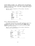 Area 13. Manokin River
In sharp contrast to the complete absence of SAV in the nearby Nanticoke
and Wiconrico Rivers after 1971, the MBHRL Survey indicated Ruppia from 1971
through 1976 and Zostera from 1971 to 1975 in the Manokin River (see Table 41)
However, percentage occurrence based on number of vegetated sampling stations
indicates declines for both species over time. Zostera was documented at 33
percent of the 15 sampling stations in 1971, 7 percent in 1975 and zero in
1976. Ruppia's decline was less drastic; 20 percent of the stations were
vegetated in 1971, 7 percent in 1975 and almost 7 percent in 1976. In 1972,
P_. pectinatus was documented at the mouths of league and Goose Creeks but has
not been found since then.
Table 41. Historic documentation of SAV by decades, Manokin River,
Maryland (Area 13)
Species 1960 1970
Ruppia
marl ti ma 1967(V) 1971-1976(MB)
Zostera
marina 1967(V) 1971-1975(MB)
Potamogeton
pectinatus 1972(MB)
Area 14. Patapsco River
Ruppia and Elodea are documented with herbarium specimens from the 1950s;
however, there is no documented evidence of Elodea since then (see Table 42).
Ruppia was noted as occasional in Main Creek in 1961 by the Milfoil Survey
personnel and was found to be locally abundant in Back Creek. MBHRL teams
have not observed Ruppia or Elodea in the Patapsco River during their six
years of sampling.
In 1961, Myriophyllum was found to be locally abundant in Main Creek and
occasional to rare in Back, Rock and Fox Creeks. IP. perfoliatus was consider-
ed to be generally rare, though locally abundant in Back Creek. Vallisneria,
the only other SAV species observed in 1961, was locally abundant in Back Creek
and rare to occasional in all other creeks that were sampled.
There is no information indicating any sampling of SAV in the Patapsco
River from 1962 to 1971 except for one herbarium specimen for Najas dated
1968. The MBHRL Survey teams have documented three species from 1972 to 1976,
the two Potamogeton spp. andVallisneria. However, data indicate only trace
amounts of all three species except for Vallisneria in 1974, when analysis was
indicated as 99 percent per volume from two samples near the mouth of Stony Creek,
168
image:
Area 13. Manokin River
In sharp contrast to the complete absence of SAV in the nearby Nanticoke
and Wiconrico Rivers after 1971, the MBHRL Survey indicated Ruppia from 1971
through 1976 and Zostera from 1971 to 1975 in the Manokin River (see Table 41)
However, percentage occurrence based on number of vegetated sampling stations
indicates declines for both species over time. Zostera was documented at 33
percent of the 15 sampling stations in 1971, 7 percent in 1975 and zero in
1976. Ruppia's decline was less drastic; 20 percent of the stations were
vegetated in 1971, 7 percent in 1975 and almost 7 percent in 1976. In 1972,
P_. pectinatus was documented at the mouths of league and Goose Creeks but has
not been found since then.
Table 41. Historic documentation of SAV by decades, Manokin River,
Maryland (Area 13)
Species 1960 1970
Ruppia
marl ti ma 1967(V) 1971-1976(MB)
Zostera
marina 1967(V) 1971-1975(MB)
Potamogeton
pectinatus 1972(MB)
Area 14. Patapsco River
Ruppia and Elodea are documented with herbarium specimens from the 1950s;
however, there is no documented evidence of Elodea since then (see Table 42).
Ruppia was noted as occasional in Main Creek in 1961 by the Milfoil Survey
personnel and was found to be locally abundant in Back Creek. MBHRL teams
have not observed Ruppia or Elodea in the Patapsco River during their six
years of sampling.
In 1961, Myriophyllum was found to be locally abundant in Main Creek and
occasional to rare in Back, Rock and Fox Creeks. IP. perfoliatus was consider-
ed to be generally rare, though locally abundant in Back Creek. Vallisneria,
the only other SAV species observed in 1961, was locally abundant in Back Creek
and rare to occasional in all other creeks that were sampled.
There is no information indicating any sampling of SAV in the Patapsco
River from 1962 to 1971 except for one herbarium specimen for Najas dated
1968. The MBHRL Survey teams have documented three species from 1972 to 1976,
the two Potamogeton spp. andVallisneria. However, data indicate only trace
amounts of all three species except for Vallisneria in 1974, when analysis was
indicated as 99 percent per volume from two samples near the mouth of Stony Creek,
168
image:
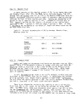 Table 42. Historic documentation of SAV by decades, Patapsco River,
Maryland (Area 14)
Species
Potamogeton
perfoliatus
Ruppia
maritima
Myriophyllum
spicatum
P. pectinatus
Vallisneria
amencana
Elodea
canadensis
1950 1960
1961(M)
1953(H) 1961(M)
1961(M)
1961(M)
1950(H)
1970a
1972-1974(MB)
1972(MB)
1973-1974(MB)
1976(MB)
1968(H)
aMBHRL did not sample the Patapsco River in 1975
Area 15. Big and Ljittle Annemessex Rivers
Ruppia and Zostera are documented as the dominant species in the
Annemessex Rivers (see Table 43). Both species were documented from 1959 to
1961 during the Benthic Survey and have been found consistently over the six
years of the MBHRL Survey. However, percentage occurrence of sampling stations
indicates that both species have declined since 1971; Ruppia was found at 45
percent of the 20 stations in 1971 and at 25 percent in 1976; and Zostera de-
clined from 60 percent in 1971 to 15 percent in 1976.
Table 43. Historic documentation of SAV by decades, Big and Little
Annemessex Rivers, Maryland (Area 15)
Species
Ruppia
maritima
Zostera
marina
Potamogeton
perfoliatus
1960
1959-1961(6)
1967(V)
1959-1961(6)
1967(V)
1967(V)
1970
1971-1976(MB)
1971-1976(MB)
1971-1973(MB)
169
image:
Table 42. Historic documentation of SAV by decades, Patapsco River,
Maryland (Area 14)
Species
Potamogeton
perfoliatus
Ruppia
maritima
Myriophyllum
spicatum
P. pectinatus
Vallisneria
amencana
Elodea
canadensis
1950 1960
1961(M)
1953(H) 1961(M)
1961(M)
1961(M)
1950(H)
1970a
1972-1974(MB)
1972(MB)
1973-1974(MB)
1976(MB)
1968(H)
aMBHRL did not sample the Patapsco River in 1975
Area 15. Big and Ljittle Annemessex Rivers
Ruppia and Zostera are documented as the dominant species in the
Annemessex Rivers (see Table 43). Both species were documented from 1959 to
1961 during the Benthic Survey and have been found consistently over the six
years of the MBHRL Survey. However, percentage occurrence of sampling stations
indicates that both species have declined since 1971; Ruppia was found at 45
percent of the 20 stations in 1971 and at 25 percent in 1976; and Zostera de-
clined from 60 percent in 1971 to 15 percent in 1976.
Table 43. Historic documentation of SAV by decades, Big and Little
Annemessex Rivers, Maryland (Area 15)
Species
Ruppia
maritima
Zostera
marina
Potamogeton
perfoliatus
1960
1959-1961(6)
1967(V)
1959-1961(6)
1967(V)
1967(V)
1970
1971-1976(MB)
1971-1976(MB)
1971-1973(MB)
169
image:
 Potamogeton pectjnatus is the only other species whose presence has
been documented in this area. During the 1967 Vegetation Survey, 69 percent
of the stations sampled in the Big Annemessex River were vegetated with
P.. pectinatus. Trace amounts were noted in MBHRL analyses of 1971 and 1973
samples from the Little Annemessex. In 1972, the species was found in "greater
than trace" (Kerwin et al. 1975b) amounts at several stations in the Big
Annemessex in Fords and Crane Coves.
Area 16. Gunpowder and Bush Rivers
Historic records for the Gunpowder and Bush Rivers date back to herbarium
specimens of 1895 for Myriophyllum, P_. perfoliatus and P_. pectinatus (see
Table 44). There is no indication that £_. pectinatus and Ruppia (documented
in 1902 and 1903 only) were able to successfully persist. Milfoil Surveys
and herbarium specimens documented a total of eight SAV species in this area
during the 1960s. In 1970 and 1971, five of these same species were found.
However, since 1971, MBHRL has documented no vegetation in the headwaters of
the two rivers. MBHRL has not sampled the southern portions of the rivers.
Elser (1969) surveyed the Bird River in 1965 and found large beds of
Myriophyllum.Vallisneria and Ceratophyllum. When milfoil retreated the
following year, Vallisneria and Ceratophyllum colonized the vacated areas.
However, in 1967, the same areas were noted to be nearly bare with only a few
sparse beds.
Table 44. Historic documentation of SAV by decades, Gunpowder and
Bush Rivers, Maryland (Area 16)
Species
Potamogeton
perfoliatus
Ruppi a
maritima
Hyriophyllum
spicatum
1890
1895(H)
1895(H)
1900 1950
1902(H)
190Z(H)
1903(H)
1960
1961(H)(M)
1960,1961(H)
1962,1963(H)
1970
1970-1971(M)
1970(H)
1971(W)
P_. pectinatus 1895(H)
Zannichellia
palustris
Vallisneria
americana
El odea
canadensis
Najas spp.
Chara spp.
Cerataphyllum
demersum
1902(H)
1951(H)
1956(H)
1956(H)
1956(H)
1964-1967(E)
1961(M)
1967-1969(M)
1961(M)
1961,1963(H
1965-1967(E
1961,1969(M)
1961(M)
1961(M)
1963(H)
1961(M)
1961(H)
1965-1967(E)
1970-1971(M)
1970-1971(M)
1971(M)
1970-1971(N)
1970-1971{M)
170
image:
Potamogeton pectjnatus is the only other species whose presence has
been documented in this area. During the 1967 Vegetation Survey, 69 percent
of the stations sampled in the Big Annemessex River were vegetated with
P.. pectinatus. Trace amounts were noted in MBHRL analyses of 1971 and 1973
samples from the Little Annemessex. In 1972, the species was found in "greater
than trace" (Kerwin et al. 1975b) amounts at several stations in the Big
Annemessex in Fords and Crane Coves.
Area 16. Gunpowder and Bush Rivers
Historic records for the Gunpowder and Bush Rivers date back to herbarium
specimens of 1895 for Myriophyllum, P_. perfoliatus and P_. pectinatus (see
Table 44). There is no indication that £_. pectinatus and Ruppia (documented
in 1902 and 1903 only) were able to successfully persist. Milfoil Surveys
and herbarium specimens documented a total of eight SAV species in this area
during the 1960s. In 1970 and 1971, five of these same species were found.
However, since 1971, MBHRL has documented no vegetation in the headwaters of
the two rivers. MBHRL has not sampled the southern portions of the rivers.
Elser (1969) surveyed the Bird River in 1965 and found large beds of
Myriophyllum.Vallisneria and Ceratophyllum. When milfoil retreated the
following year, Vallisneria and Ceratophyllum colonized the vacated areas.
However, in 1967, the same areas were noted to be nearly bare with only a few
sparse beds.
Table 44. Historic documentation of SAV by decades, Gunpowder and
Bush Rivers, Maryland (Area 16)
Species
Potamogeton
perfoliatus
Ruppi a
maritima
Hyriophyllum
spicatum
1890
1895(H)
1895(H)
1900 1950
1902(H)
190Z(H)
1903(H)
1960
1961(H)(M)
1960,1961(H)
1962,1963(H)
1970
1970-1971(M)
1970(H)
1971(W)
P_. pectinatus 1895(H)
Zannichellia
palustris
Vallisneria
americana
El odea
canadensis
Najas spp.
Chara spp.
Cerataphyllum
demersum
1902(H)
1951(H)
1956(H)
1956(H)
1956(H)
1964-1967(E)
1961(M)
1967-1969(M)
1961(M)
1961,1963(H
1965-1967(E
1961,1969(M)
1961(M)
1961(M)
1963(H)
1961(M)
1961(H)
1965-1967(E)
1970-1971(M)
1970-1971(M)
1971(M)
1970-1971(N)
1970-1971{M)
170
image:
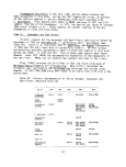 When Milfoil Survey teams looked at Gunpowder River in 1969, 1970 and
1971, Myriophyllum was found to be dominant south of the railroad bridge.
Vallisneria and P_. perfoliatus were found along with traces of Najas and
Ceratophyllum. In Dundee and Saltpeter Creeks, the water was observed to
be only slightly turbid in May and June of 1960. Shoal areas were covered
with extensive diversified growth. The excessive rains and runoff in July
seemed to affect the vegetation in Saltpeter Creek resulting in almost com-
plete loss. Dundee Creek was not as affected and extensive beds of
Myriophyllum and Vallisneria were noted. In July of 1977, MBHRL Survey teams
found abundant Vallisneria and Chara in Dundee Creek. Myriophyllum and
£_. crispus were observed growing in water over 2 m deep.
Potamogeton foliosus, a specie^ that had not been seen for about 10
years, was noted in the Gunpowder River in 1971. The MBHRL Survey did not
indicate the continued presence of this species subsequent to the scattered
growth that was noted by the Milfoil team.
Area 17. Pocomoke Sound
The Vegetation Survey sampled 19 transects in Pocomoke Sound in 1967 and
documented Zostera at 89 percent and Ruppia at 58 percent of the stations
(see Table 45). Except for 1974, MBHRL Survey teams have sampled from 20 to
22 stations each year in the Maryland portion of Pocomoke Sound. As would be
expected in the high salinity waters of the Sound, Ruppia and Zostera were
the only species documented. Based on percentage occurrence figures, both
species show declines over the six year MBHRL Survey. Zostera was observed
at 18 percent of the stations sampled in 1971 compared to 9 percent in 1976.
Ruppia declined from 9 percent to 4.5 percent over the same six years and
was noted at all in 1972 and 1973.
Table 45. Historic documentation of SAV by decades Pocomoke Sound,
Maryland (Area 17)
Species 1960 1970a
Ruppia 1967(V) 1971,1975-1976(MB)
maritima
Zostera 1967(V) 1971-1973(MB)
marina 1975-1976(MB)
'MBHRL did not sample Pocomoke Sound in 1974
171
image:
When Milfoil Survey teams looked at Gunpowder River in 1969, 1970 and
1971, Myriophyllum was found to be dominant south of the railroad bridge.
Vallisneria and P_. perfoliatus were found along with traces of Najas and
Ceratophyllum. In Dundee and Saltpeter Creeks, the water was observed to
be only slightly turbid in May and June of 1960. Shoal areas were covered
with extensive diversified growth. The excessive rains and runoff in July
seemed to affect the vegetation in Saltpeter Creek resulting in almost com-
plete loss. Dundee Creek was not as affected and extensive beds of
Myriophyllum and Vallisneria were noted. In July of 1977, MBHRL Survey teams
found abundant Vallisneria and Chara in Dundee Creek. Myriophyllum and
£_. crispus were observed growing in water over 2 m deep.
Potamogeton foliosus, a specie^ that had not been seen for about 10
years, was noted in the Gunpowder River in 1971. The MBHRL Survey did not
indicate the continued presence of this species subsequent to the scattered
growth that was noted by the Milfoil team.
Area 17. Pocomoke Sound
The Vegetation Survey sampled 19 transects in Pocomoke Sound in 1967 and
documented Zostera at 89 percent and Ruppia at 58 percent of the stations
(see Table 45). Except for 1974, MBHRL Survey teams have sampled from 20 to
22 stations each year in the Maryland portion of Pocomoke Sound. As would be
expected in the high salinity waters of the Sound, Ruppia and Zostera were
the only species documented. Based on percentage occurrence figures, both
species show declines over the six year MBHRL Survey. Zostera was observed
at 18 percent of the stations sampled in 1971 compared to 9 percent in 1976.
Ruppia declined from 9 percent to 4.5 percent over the same six years and
was noted at all in 1972 and 1973.
Table 45. Historic documentation of SAV by decades Pocomoke Sound,
Maryland (Area 17)
Species 1960 1970a
Ruppia 1967(V) 1971,1975-1976(MB)
maritima
Zostera 1967(V) 1971-1973(MB)
marina 1975-1976(MB)
'MBHRL did not sample Pocomoke Sound in 1974
171
image:
 Area 18. Magothy River
In the Magothy River, Milfoil Survey teams, Vernon Stotts, Harold Elser
and MBHRL have documented nine species of SAV over the 17-year period from
1960 to 1976 (see Table 46). A saltwater intrusion noted prior to 1967 and
allowed SAV species other than Myriophyllum to become reestablished (Elser
1969). Ruppia and P_. perfoliatus were found in 1969 to be dominant in such
areas as the shoals off Broad Creek, in Deep Mill Creek and in the upper
reaches of Blackhole Creek. In the embayments beyond the confluence of Cockey,
Magothy, and Cattail Creeks, the water was very turbid in August, 1969, and
almost no SAV was noted by the Milfoil Survey team personnel.
P_. perfoliatus was documented consistently until 1974 when it was last
observed at two locations off Park and Grays Points. Ruppia, Chara and
Najas have not been documented since 1974 despite annual sampling efforts by
MBHRL. Only Vallisneria has been noted in the Magothy River since 1974 and
1976 when only a trace amount was noted off Pea Patch Point.
Table 46. Historic documentation of SAV by decades, Magothy River,
Maryland (Area 18)
Species 1900
Potamogeton
perfoliatus
Ruopia
maritime
Myriophyllum
spicatum
P. pectinatus
1940 1950
1945(H) 1950(H)
1959(B)a
1945(H) 1950(H)
1959(8)
1960
1960-1961(B)
1961,1969(M)
1969(E)
1960-1961(8)
1961,1969(M)
1961(M)
1968-1969(M)
1967(E)
1960(B)
1961,1969(M)
1970
1971(MB)
1973-1974(MB)
1970-1971(M)
1971,1974(MB)
1970-1971(M)
1970(H)
1970-1971(M)
1970-1971(M)
1971,1973(MB)
Zannichellia
palustris
Vallisneria 1902(H)
americana
El odea
cafiadensis
Na^'as spp.
Chfrra spp.
Ceratophyll urn 1947(H)
denier sum
1960-1961(6)
1961(M)
1961(M)
1960-1961(8)
1961(M)
1961(B)(M)
1970-1971(M)
1970-1971(M)
1971,1973(MB)
1976(MB)
1971(MB)
1973-1974(MB)
1974(MB)
aThe 1959 Benthic Survey listed Potamogeton sp. by genus only
172
image:
Area 18. Magothy River
In the Magothy River, Milfoil Survey teams, Vernon Stotts, Harold Elser
and MBHRL have documented nine species of SAV over the 17-year period from
1960 to 1976 (see Table 46). A saltwater intrusion noted prior to 1967 and
allowed SAV species other than Myriophyllum to become reestablished (Elser
1969). Ruppia and P_. perfoliatus were found in 1969 to be dominant in such
areas as the shoals off Broad Creek, in Deep Mill Creek and in the upper
reaches of Blackhole Creek. In the embayments beyond the confluence of Cockey,
Magothy, and Cattail Creeks, the water was very turbid in August, 1969, and
almost no SAV was noted by the Milfoil Survey team personnel.
P_. perfoliatus was documented consistently until 1974 when it was last
observed at two locations off Park and Grays Points. Ruppia, Chara and
Najas have not been documented since 1974 despite annual sampling efforts by
MBHRL. Only Vallisneria has been noted in the Magothy River since 1974 and
1976 when only a trace amount was noted off Pea Patch Point.
Table 46. Historic documentation of SAV by decades, Magothy River,
Maryland (Area 18)
Species 1900
Potamogeton
perfoliatus
Ruopia
maritime
Myriophyllum
spicatum
P. pectinatus
1940 1950
1945(H) 1950(H)
1959(B)a
1945(H) 1950(H)
1959(8)
1960
1960-1961(B)
1961,1969(M)
1969(E)
1960-1961(8)
1961,1969(M)
1961(M)
1968-1969(M)
1967(E)
1960(B)
1961,1969(M)
1970
1971(MB)
1973-1974(MB)
1970-1971(M)
1971,1974(MB)
1970-1971(M)
1970(H)
1970-1971(M)
1970-1971(M)
1971,1973(MB)
Zannichellia
palustris
Vallisneria 1902(H)
americana
El odea
cafiadensis
Na^'as spp.
Chfrra spp.
Ceratophyll urn 1947(H)
denier sum
1960-1961(6)
1961(M)
1961(M)
1960-1961(8)
1961(M)
1961(B)(M)
1970-1971(M)
1970-1971(M)
1971,1973(MB)
1976(MB)
1971(MB)
1973-1974(MB)
1974(MB)
aThe 1959 Benthic Survey listed Potamogeton sp. by genus only
172
image:
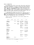 Area 19. Severn River
Submerged aquatic species have been documented in the Severn River since
1893 (see Table 47). In the 1950s and 1960s, Milfoil Survey and herbarium
records show 8 species present. Survey teams found abundant Elodea in July,
1961, along the south shore of the river. Elser (1969) found abundant
£. perfoliatus and Myriophyllum prior to August, 1966. By 1967, Elser noted
only a few, sparse beds of the same species. In September, 1969, the waters
of the Servern River were found to be cloudy in most embayments and indentations.
In Asquith Creek and Ringold Cove abundant growth of £. perfoliatus was ob-
served along with scattered _R_uppia and P. pectinatus. Across the river, SAV
seemed to be practically nonexistent. In the Severna Park area and across the
river in creek embayments above Long Point, scattered growth of P.. perfoliatus
and Ruppia were commonly found. By 1969, no vegetation was observed in the
upper reaches of the river. P.. perfoliatus appeared to be the dominant species
in the 1970s; however, between 1971 and 1976 percentage occurrence figures
indicated a dec!ine of about one-half in the number of vegetated stations.
Table 47. Historic documentation of SAV by decades, Severn River,
Maryland (Area 19)
Species
1890
1920
1940
1950
1960
Ceratophyllum
demersum
1949(H) 1952(H)
1970
Potamogeton 1927(H)
perfoliatus
Ruppia 1927(H)
maritime
Mynqphyllum
spicatum
P. pectinatus 1893(H) 1927(H)
Zannichellia
palustris
Vail isneria
amencana
Elodea
canadensis
Najas spp.
Chara spp.
1952(H) 1961,1969(M)
1966-1967(E)
1952(H) 1961,1969(M)
1961(M)
1966-1967(E)
1968-1969(M)
1952(H) 1961,1969(M)
1961(M)
1947(H) 1952(H) 1961(M)
1954(H) 1961(M)
1969(H)
1961(M)
1970-1971(M)
1976(MB)
1971-1974(MB)
1970-1971(M)
1971-1974(MB)
1976(MB)
1970(H)
1970-1971(M)
1972,1976(MB)
1970-1971(M)
1972-1974(MB)
1970-1971(M)
1974,1976(MB)
1970-1971(M)
1971-1974(MB)
1972-1974(MB)
1976(MB)
1974(MB)
aMBHRL did not sample the Severn River in 1975
173
image:
Area 19. Severn River
Submerged aquatic species have been documented in the Severn River since
1893 (see Table 47). In the 1950s and 1960s, Milfoil Survey and herbarium
records show 8 species present. Survey teams found abundant Elodea in July,
1961, along the south shore of the river. Elser (1969) found abundant
£. perfoliatus and Myriophyllum prior to August, 1966. By 1967, Elser noted
only a few, sparse beds of the same species. In September, 1969, the waters
of the Servern River were found to be cloudy in most embayments and indentations.
In Asquith Creek and Ringold Cove abundant growth of £. perfoliatus was ob-
served along with scattered _R_uppia and P. pectinatus. Across the river, SAV
seemed to be practically nonexistent. In the Severna Park area and across the
river in creek embayments above Long Point, scattered growth of P.. perfoliatus
and Ruppia were commonly found. By 1969, no vegetation was observed in the
upper reaches of the river. P.. perfoliatus appeared to be the dominant species
in the 1970s; however, between 1971 and 1976 percentage occurrence figures
indicated a dec!ine of about one-half in the number of vegetated stations.
Table 47. Historic documentation of SAV by decades, Severn River,
Maryland (Area 19)
Species
1890
1920
1940
1950
1960
Ceratophyllum
demersum
1949(H) 1952(H)
1970
Potamogeton 1927(H)
perfoliatus
Ruppia 1927(H)
maritime
Mynqphyllum
spicatum
P. pectinatus 1893(H) 1927(H)
Zannichellia
palustris
Vail isneria
amencana
Elodea
canadensis
Najas spp.
Chara spp.
1952(H) 1961,1969(M)
1966-1967(E)
1952(H) 1961,1969(M)
1961(M)
1966-1967(E)
1968-1969(M)
1952(H) 1961,1969(M)
1961(M)
1947(H) 1952(H) 1961(M)
1954(H) 1961(M)
1969(H)
1961(M)
1970-1971(M)
1976(MB)
1971-1974(MB)
1970-1971(M)
1971-1974(MB)
1976(MB)
1970(H)
1970-1971(M)
1972,1976(MB)
1970-1971(M)
1972-1974(MB)
1970-1971(M)
1974,1976(MB)
1970-1971(M)
1971-1974(MB)
1972-1974(MB)
1976(MB)
1974(MB)
aMBHRL did not sample the Severn River in 1975
173
image:
 Area 20. Patuxent River
From the 1930s to present, eight species of SAV were documented in the
Patuxent River (see Table 48). Elser (1969) observed healthy Zostera at
Solomons in the late 1940s. Stewart (1962) listed P_. pectinatus plus unnamed
salt-water species as present in the lower Patuxent River from the mouth
upstream to Point Patience. Herbarium specimens plus the sampling work of
the Milfoil Survey and Vernon Stotts provide evidence of occurrence in the
1960s. In July, 1961, Milfoil teams sampled the west side of the Patuxent
River south of the Benedict Bridge and noted Elodea to be generally abundant
in most of the creeks. Ruppia and £_. perfoliatus ranged from rare to abundant,
£. pectinatus was observed to be locally abundant in St. Thomas and Cuckold
Creeks and Zannichellia was listed as rare in Mill and Washington Creeks.
Table 48. Historic documentation of SAV by decades, Patuxent River.
Maryland (Area 20)
Species
Potamogeton
perfoliatus
Ruppia
maritima
Zostera
marina
P. pectinatus
Zannichellia
palustris
Elodea
canadensis
1930 1940 1950 1960
1952(H) 1961(M)
1961,1964(H)
1966(H)
1963-1965(A)
1937(H) 1946(H) 1961(M)
1963-1965(A)
1933,1937(H) 1940s(E) 1961(8)
1946(H) 1965(H)
1937(H) 1946(H) 1950s(RC) 1961(M)
1961(M)
1965(H)
1954(H) 1961(M)
1965(H)
1970
1970-1971(M)
1970-1971(M)
1972,1974(MB)
1976(MB)
1971(MB)
1970-1971(M)
Najas spp.
Vallisneria
americana
1939(H)
1947(H)
1954(H)
1957(H)
1969(H)
1965(H)
The east side of the river near Solomons was also sampled in July, 1961.
Vegetation was limited to Ruppia and was found to be generally sparse. MBHRL
and Milfoil surveys from 1970 to 1976 documented only three of the eight species
that had been observed during the previous decade. A trace of Zostera was noted
in Cuckold Creek in 1971. Milfoil Survey teams described a general lack of
extensive vegetation in the entire river and only sparse growths of Ruppia,
IP. pectinatus and IP. perfoliatus in 1970 and 1971. Trace amounts of Ruppia
were documented in 1972 off Sheridan Point and in Cuckold Creek.
was found again in.1974 and 1976 at the Cukold Creek station.
Area 21. Back, Middle and Gunpowder Rivers
Only Ruppia
Submerged aquatic species diversity was high in the 1960s in these three
rivers; ten species were documented in 1960, 1961 and 1969 (see Table 49).
174
image:
Area 20. Patuxent River
From the 1930s to present, eight species of SAV were documented in the
Patuxent River (see Table 48). Elser (1969) observed healthy Zostera at
Solomons in the late 1940s. Stewart (1962) listed P_. pectinatus plus unnamed
salt-water species as present in the lower Patuxent River from the mouth
upstream to Point Patience. Herbarium specimens plus the sampling work of
the Milfoil Survey and Vernon Stotts provide evidence of occurrence in the
1960s. In July, 1961, Milfoil teams sampled the west side of the Patuxent
River south of the Benedict Bridge and noted Elodea to be generally abundant
in most of the creeks. Ruppia and £_. perfoliatus ranged from rare to abundant,
£. pectinatus was observed to be locally abundant in St. Thomas and Cuckold
Creeks and Zannichellia was listed as rare in Mill and Washington Creeks.
Table 48. Historic documentation of SAV by decades, Patuxent River.
Maryland (Area 20)
Species
Potamogeton
perfoliatus
Ruppia
maritima
Zostera
marina
P. pectinatus
Zannichellia
palustris
Elodea
canadensis
1930 1940 1950 1960
1952(H) 1961(M)
1961,1964(H)
1966(H)
1963-1965(A)
1937(H) 1946(H) 1961(M)
1963-1965(A)
1933,1937(H) 1940s(E) 1961(8)
1946(H) 1965(H)
1937(H) 1946(H) 1950s(RC) 1961(M)
1961(M)
1965(H)
1954(H) 1961(M)
1965(H)
1970
1970-1971(M)
1970-1971(M)
1972,1974(MB)
1976(MB)
1971(MB)
1970-1971(M)
Najas spp.
Vallisneria
americana
1939(H)
1947(H)
1954(H)
1957(H)
1969(H)
1965(H)
The east side of the river near Solomons was also sampled in July, 1961.
Vegetation was limited to Ruppia and was found to be generally sparse. MBHRL
and Milfoil surveys from 1970 to 1976 documented only three of the eight species
that had been observed during the previous decade. A trace of Zostera was noted
in Cuckold Creek in 1971. Milfoil Survey teams described a general lack of
extensive vegetation in the entire river and only sparse growths of Ruppia,
IP. pectinatus and IP. perfoliatus in 1970 and 1971. Trace amounts of Ruppia
were documented in 1972 off Sheridan Point and in Cuckold Creek.
was found again in.1974 and 1976 at the Cukold Creek station.
Area 21. Back, Middle and Gunpowder Rivers
Only Ruppia
Submerged aquatic species diversity was high in the 1960s in these three
rivers; ten species were documented in 1960, 1961 and 1969 (see Table 49).
174
image:
 By 1970, diversity had decreased to six species with the loss of Najas,
IP. pectinatus, Chara and Zannichellia. Good growths of Vallisneria were
seen in Galloway Creek in 1969 with lesser amounts of P_. perfoliatus and
traces of Zannichellia, P_. pectinatus, Ruppia and Najas. The following year,
scattered patches of Vallisneria and Ruppia and some of the other pondweeds
were noted throughout Middle River.
Table 49. Historic documentation of SAV by decades, Back, Middle
and Gunpowder Rivers, Maryland (Area 21)
Species
1940
1960
1970
Potamogeton
perfoliatus
Ruppia
maritima
Myriophyllum
spicatum
P. pectinatus
Zannichellia
palustris
Vallisneria
amencana
Elodea
canadensis
Najas spp.
Chara spp.
Ceratophyllum
demersum
1940(H) 1960-1961 ,1969(M)
1961,1969(M)
1960-1961(6)
1960-1961 ,1969(M)
1962,1963(H)
1967-1969(50)
1968(H)
1960-1961, 1969(M)
1963(H)
1969(M)
1940(H) 1960-1961(6)
1960-1961, 1969(M)
1940(H) 1960-1961, 1969(M)
1960-1961, 1969(M)
1961(6)
1960(M)
1940(H) 1960-1961, 1969(M)
1970-1971(M)
1970(M)
197UHB)
1970-1971(M)
1971-1973, 1975(M6)
1970-1971(M)
1974-1975(M8)
1970-1971(M)
1972(M6)
1970-1971(M)
Back River was Reported to be very turbid in 1969 and no submerged
vegetation was documented. Vallisneria showed up in 1974 and 1975 but not
in 1976 at the mouth of Seneca Creek. Ruppia was documented in the same
area in Seneca Creek by MBHRL in 1971 but has not been found since. Along
with Vallisneria, Myriophyllum is the only other SAV species that was seen
in 1975. The 1976 MBHRL Survey found no vegetation in Area 21.
Area 22. Curtis and Cove Points
Herbarium specimens and Benthic Survey transects taken along the western
Bay shore between Curtis and Cove Points have documented four SAV species be-
tween 1931 and 1965 (see Table 50). Despite about 20 stations sampled from
1971 to 1976, the MBHRL teams found no vegetation. Although the high energy
nature of this portion of the Chesapeake Bay is not conducive to SAV invasion
and growth, it is interesting to note that there are past records of species
occurrence in these a^reas.
175
image:
By 1970, diversity had decreased to six species with the loss of Najas,
IP. pectinatus, Chara and Zannichellia. Good growths of Vallisneria were
seen in Galloway Creek in 1969 with lesser amounts of P_. perfoliatus and
traces of Zannichellia, P_. pectinatus, Ruppia and Najas. The following year,
scattered patches of Vallisneria and Ruppia and some of the other pondweeds
were noted throughout Middle River.
Table 49. Historic documentation of SAV by decades, Back, Middle
and Gunpowder Rivers, Maryland (Area 21)
Species
1940
1960
1970
Potamogeton
perfoliatus
Ruppia
maritima
Myriophyllum
spicatum
P. pectinatus
Zannichellia
palustris
Vallisneria
amencana
Elodea
canadensis
Najas spp.
Chara spp.
Ceratophyllum
demersum
1940(H) 1960-1961 ,1969(M)
1961,1969(M)
1960-1961(6)
1960-1961 ,1969(M)
1962,1963(H)
1967-1969(50)
1968(H)
1960-1961, 1969(M)
1963(H)
1969(M)
1940(H) 1960-1961(6)
1960-1961, 1969(M)
1940(H) 1960-1961, 1969(M)
1960-1961, 1969(M)
1961(6)
1960(M)
1940(H) 1960-1961, 1969(M)
1970-1971(M)
1970(M)
197UHB)
1970-1971(M)
1971-1973, 1975(M6)
1970-1971(M)
1974-1975(M8)
1970-1971(M)
1972(M6)
1970-1971(M)
Back River was Reported to be very turbid in 1969 and no submerged
vegetation was documented. Vallisneria showed up in 1974 and 1975 but not
in 1976 at the mouth of Seneca Creek. Ruppia was documented in the same
area in Seneca Creek by MBHRL in 1971 but has not been found since. Along
with Vallisneria, Myriophyllum is the only other SAV species that was seen
in 1975. The 1976 MBHRL Survey found no vegetation in Area 21.
Area 22. Curtis and Cove Points
Herbarium specimens and Benthic Survey transects taken along the western
Bay shore between Curtis and Cove Points have documented four SAV species be-
tween 1931 and 1965 (see Table 50). Despite about 20 stations sampled from
1971 to 1976, the MBHRL teams found no vegetation. Although the high energy
nature of this portion of the Chesapeake Bay is not conducive to SAV invasion
and growth, it is interesting to note that there are past records of species
occurrence in these a^reas.
175
image:
 Table 50. Historic documentation of SAV by decades, Curtis and Cove
Points, Maryland (Area 22)
Species
Potamogeton
perfoliatus
Ruppia
maritima
Zostera
manna
Zannichellia
palustris
1930 1940 1960
1963(H)
1948(H) 1961(B)
1965(H)
1931(H)
Area 23. South, West and Rhode Rivers
Elser (1969, p. 58) reported that the Rhode River supported" rather
heavy weed load..." in 1964. Myriophyllum was dominant but the river also
included large beds of P_. perfoliatus and lesser amounts of El odea, P_. pectinatus.
Ruppia and Zannichellia were also represented (see Table 51). In 1965, Elser
observed; a general decline of vegetation over the summer. By 1966, SAV coverage
appeared to be about 10 percent of the 1965 observed abundance. By 1967, Elser
found only a few sparse beds of P_- oerfoliatus. This decline Elser referred to
as a phenomenon and named it the "Rhode River Evanescence."
Southwick and Pine (1975) studied the complete shoreline of the Rhode River
and its tributaries from 1966 to 1973. Based on their observations, they con-
cluded that the six species studied had declined substantially and El odea had
disappeared completely after 1966. Those species that were observed until 1973
were Ruppia, £_. perfoliatus. Myriophyllum and Zannichellia. In 1961, the
Milfoil Survey teams surveyed the Rhode River and observed P_. perfoliatus grow-
ing abundantly in most of the creeks. Elodea and Ruppia were considered as
occasional to common inhabitants of the same area. A 1945 herbarium specimen
places Vallisneria in the Rhode River but subsequent survey work has not docu-
mented the species since. In 1969, P.. perfoliatus was still observed to be
abundant. Lesser amounts of £. pectinatus. Ruppia and a trace of Myriophyllum
were noted prior to a mid-July die-back. MBHRL Survey teams did not find any
vegetation from 1971 to 1976.
Milfoil teams surveyed West River in August of 1961 and found P_. perfoliatus
to be growing abundantly in most of the sheltered areas of the river. Elodea
and Ruppia were considered common in most creeks and Myriophyllum and
P.- pectinatus turned up occasionally. Ruppia showed up in West River in 1976,
Tor the first time since MBHRL started surveying in 1971.
176
image:
Table 50. Historic documentation of SAV by decades, Curtis and Cove
Points, Maryland (Area 22)
Species
Potamogeton
perfoliatus
Ruppia
maritima
Zostera
manna
Zannichellia
palustris
1930 1940 1960
1963(H)
1948(H) 1961(B)
1965(H)
1931(H)
Area 23. South, West and Rhode Rivers
Elser (1969, p. 58) reported that the Rhode River supported" rather
heavy weed load..." in 1964. Myriophyllum was dominant but the river also
included large beds of P_. perfoliatus and lesser amounts of El odea, P_. pectinatus.
Ruppia and Zannichellia were also represented (see Table 51). In 1965, Elser
observed; a general decline of vegetation over the summer. By 1966, SAV coverage
appeared to be about 10 percent of the 1965 observed abundance. By 1967, Elser
found only a few sparse beds of P_- oerfoliatus. This decline Elser referred to
as a phenomenon and named it the "Rhode River Evanescence."
Southwick and Pine (1975) studied the complete shoreline of the Rhode River
and its tributaries from 1966 to 1973. Based on their observations, they con-
cluded that the six species studied had declined substantially and El odea had
disappeared completely after 1966. Those species that were observed until 1973
were Ruppia, £_. perfoliatus. Myriophyllum and Zannichellia. In 1961, the
Milfoil Survey teams surveyed the Rhode River and observed P_. perfoliatus grow-
ing abundantly in most of the creeks. Elodea and Ruppia were considered as
occasional to common inhabitants of the same area. A 1945 herbarium specimen
places Vallisneria in the Rhode River but subsequent survey work has not docu-
mented the species since. In 1969, P.. perfoliatus was still observed to be
abundant. Lesser amounts of £. pectinatus. Ruppia and a trace of Myriophyllum
were noted prior to a mid-July die-back. MBHRL Survey teams did not find any
vegetation from 1971 to 1976.
Milfoil teams surveyed West River in August of 1961 and found P_. perfoliatus
to be growing abundantly in most of the sheltered areas of the river. Elodea
and Ruppia were considered common in most creeks and Myriophyllum and
P.- pectinatus turned up occasionally. Ruppia showed up in West River in 1976,
Tor the first time since MBHRL started surveying in 1971.
176
image:
 Table 51. Historic documentation of SAV by decades, South, West and
Rhode Rivers, Maryland (Area 23)
Species
1900
1940
1950
1960
1970
Potamogeton
perfoliatus
Ruppia
maritima
Myriophyllum
spicatum
P. pectinatus
ZannicheTlia
palustris
Vanisneria
americana
El odea
canadensis
1960,1963(H)
1961,1969(M)
1962(P&B)
1964-1967(E)
1966-1969(S&P)
1905(H) 1946(H) 1953(H) 1961,1969(M)
1962(P&B)
1963(H)
1966-1969(S&P)
1961,1968(M)
1962(P&B)
1964-1967(E)
1966-1969(S&P)
1947(H) 1961,1969(M)
1964-1967(E)
1966-1969(S&P)
1961(M)
1966-1969(S&P)
1945(H)
1945(H) 1960(H)
1961(M)
1962(P&B)
1966(S&P)
1970-1971(M)
1972-1973(S»P)
1976(CB)
1970-1971(M)
1971-1973(S&P)
1976(MB)
1976(CB)
1970(M)
1970-1973(S&P)
1971-1973(S&P)
1976(CB)
1970-1973(S&P)
1976(CB)
Phi Hipp and Brown (1965) surveyed two locations in the South River in
1962 and found dense masses of P_. perfoliatus and El odea nuttallii ringing
Limehouse Cove and from Mayo Point to Long Point. Milfoil teams found
JP. perfoliatus to be abundant in 1961 in Ramsay Lake, Selby Bay and Duvall
Creek and common to occasional growth in most of the remainder of South River.
El odea, Myriophyllum and Ruppia were determined to be generally common to the
area. MBHRL teams did not observe any vegetation in the South River from 1971
to 1976.
Personnel from the Cheapeake Bay Center for Environmental Studies (CBCES)
surveyed the Rhode River in June and July, 1976. Ruppia was determined to be
dominant, along with abundant Zannichellia. Traces of IP. perfoliatus and
£• pectinatus were also found.
Area 24. Chester River
Through the combined efforts of the Milfoil teams, MWA and MBHRL, aquatic
species occurrence and abundance in the Chester River have been well documented
from 1960 to 1976 (see Table 52). Results from the Benthic Survey (1959 to
1961) show P_. perfoliatus as dominant and abundant at virtually all stations
sampled. Najas and Myriophyllum were found frequently and P_. pectinatus and
El odea found occasionally. During 1964 through 1966, increased salinity pushed
Myriophyllum further up river and allowed P. perfoliatus to reestablish. In
177
image:
Table 51. Historic documentation of SAV by decades, South, West and
Rhode Rivers, Maryland (Area 23)
Species
1900
1940
1950
1960
1970
Potamogeton
perfoliatus
Ruppia
maritima
Myriophyllum
spicatum
P. pectinatus
ZannicheTlia
palustris
Vanisneria
americana
El odea
canadensis
1960,1963(H)
1961,1969(M)
1962(P&B)
1964-1967(E)
1966-1969(S&P)
1905(H) 1946(H) 1953(H) 1961,1969(M)
1962(P&B)
1963(H)
1966-1969(S&P)
1961,1968(M)
1962(P&B)
1964-1967(E)
1966-1969(S&P)
1947(H) 1961,1969(M)
1964-1967(E)
1966-1969(S&P)
1961(M)
1966-1969(S&P)
1945(H)
1945(H) 1960(H)
1961(M)
1962(P&B)
1966(S&P)
1970-1971(M)
1972-1973(S»P)
1976(CB)
1970-1971(M)
1971-1973(S&P)
1976(MB)
1976(CB)
1970(M)
1970-1973(S&P)
1971-1973(S&P)
1976(CB)
1970-1973(S&P)
1976(CB)
Phi Hipp and Brown (1965) surveyed two locations in the South River in
1962 and found dense masses of P_. perfoliatus and El odea nuttallii ringing
Limehouse Cove and from Mayo Point to Long Point. Milfoil teams found
JP. perfoliatus to be abundant in 1961 in Ramsay Lake, Selby Bay and Duvall
Creek and common to occasional growth in most of the remainder of South River.
El odea, Myriophyllum and Ruppia were determined to be generally common to the
area. MBHRL teams did not observe any vegetation in the South River from 1971
to 1976.
Personnel from the Cheapeake Bay Center for Environmental Studies (CBCES)
surveyed the Rhode River in June and July, 1976. Ruppia was determined to be
dominant, along with abundant Zannichellia. Traces of IP. perfoliatus and
£• pectinatus were also found.
Area 24. Chester River
Through the combined efforts of the Milfoil teams, MWA and MBHRL, aquatic
species occurrence and abundance in the Chester River have been well documented
from 1960 to 1976 (see Table 52). Results from the Benthic Survey (1959 to
1961) show P_. perfoliatus as dominant and abundant at virtually all stations
sampled. Najas and Myriophyllum were found frequently and P_. pectinatus and
El odea found occasionally. During 1964 through 1966, increased salinity pushed
Myriophyllum further up river and allowed P. perfoliatus to reestablish. In
177
image:
 1965, Milfoil personnel sampled much of the Chester River and found
7L S ? ^5: Va11is"eria' Myriophyllum and RuppTa locally dominant and
abundant. Elodea was documented occasionally. Excessive precipitation and
<±nlty IIS rUHn°ff re5UU?d in heavy clouLd water though hro^ng
nrn!?h '? J and in nnd-July and early August of 1969. In 1968, scattered
growth of £. perfoliatus was observed in the Chester River. By 1969 the
Vegetation Survey cited £. perfoliatus as dominant and abundant Ruppia and
^ynophyllum were found at Sver 50 percent of the transects sample^Tl neria
which had been found so abundant in 1968 was observed at less than 25 percent
Najas were obse™ed at over 25 percent of the
,• ^ru Survey teams documented 10 of the 11 previously seen species
in the Chester River. £. perfoliatus remained dominant through 1976. Myriophyllum
and Ceratophyll urn were the only species not found during the 1975 and 1976 surveys
£nfc hT^S °f Cer;y>phyn urn were seen in 1970 in various Chester River embly!
ments but these growths were virtually gone in 1971. Based on the frequency of
?97irtoni97fi "in ?S7iBH,Rn' t0tal VT tati°n f°r the Chester River declined^
1971 to 1976. In 1971, 60 percent of the 36 sampling stations were vegetated
as compared to 1976 when 25 percent showed vegetation. vegetated
Table 52 Historic documentation of SAV decades, Chester River,
Maryland (Area 24)
Species 1900
Potamogeton
perfoliatus
Ruppia
maritima
Myriophynum
spicatum
1940 1950 1960
1947(H) 1959(B)a 1961(M)
1965(H)
1965,1968-1969(M)
1969JV)
1947(H) 1959(B) 1960-1961(8)
1961,1965(M)
1965(H)
1969(V)
1961(B)(M)
1965,1968-1969(M)
1969(V)
1970
1970-197KM)
1971-1976(MB)
1972(H)
1970-1972(P)
1970-1971(H)
1971-1976(MB)
1970-197KM)
1971-1973(MB)
1969(V)
f. pectinatus 1907(H)
Zannichellia
palustrls
Vallisneria 1947(H)
americana
Elodea
canadensis
Najas spp. 19«(H)
Chara spp.
Ceratophyll um
demersum
1960-1961(6)
1961(H)
1969(V)
1969(V)
1961,1969(M)
1965(M)
1968(V)
1960-1961(6)
1961.1965(M)
1969(V)
1961(B)(M)
1969(V)
1961(H)
1969(V)
1961(B)
1961,1965(M)
1970-1972(P)
1970-197KM)
1971-1974, 1976(MB)
1970-1972(P)
1971(M)
1973,1976(MB)
1971, 1973, 1976(M6)
1970-197KH)
1971-1972(MB)
1975-1976(MB)
1970(M)
1970-1972(P)
1971-1976(MB)
1972-1975(MB)
1970-197KH)
aThe 1959 6enthic Survey listed Potamogeton sp. by genus only.
178
image:
1965, Milfoil personnel sampled much of the Chester River and found
7L S ? ^5: Va11is"eria' Myriophyllum and RuppTa locally dominant and
abundant. Elodea was documented occasionally. Excessive precipitation and
<±nlty IIS rUHn°ff re5UU?d in heavy clouLd water though hro^ng
nrn!?h '? J and in nnd-July and early August of 1969. In 1968, scattered
growth of £. perfoliatus was observed in the Chester River. By 1969 the
Vegetation Survey cited £. perfoliatus as dominant and abundant Ruppia and
^ynophyllum were found at Sver 50 percent of the transects sample^Tl neria
which had been found so abundant in 1968 was observed at less than 25 percent
Najas were obse™ed at over 25 percent of the
,• ^ru Survey teams documented 10 of the 11 previously seen species
in the Chester River. £. perfoliatus remained dominant through 1976. Myriophyllum
and Ceratophyll urn were the only species not found during the 1975 and 1976 surveys
£nfc hT^S °f Cer;y>phyn urn were seen in 1970 in various Chester River embly!
ments but these growths were virtually gone in 1971. Based on the frequency of
?97irtoni97fi "in ?S7iBH,Rn' t0tal VT tati°n f°r the Chester River declined^
1971 to 1976. In 1971, 60 percent of the 36 sampling stations were vegetated
as compared to 1976 when 25 percent showed vegetation. vegetated
Table 52 Historic documentation of SAV decades, Chester River,
Maryland (Area 24)
Species 1900
Potamogeton
perfoliatus
Ruppia
maritima
Myriophynum
spicatum
1940 1950 1960
1947(H) 1959(B)a 1961(M)
1965(H)
1965,1968-1969(M)
1969JV)
1947(H) 1959(B) 1960-1961(8)
1961,1965(M)
1965(H)
1969(V)
1961(B)(M)
1965,1968-1969(M)
1969(V)
1970
1970-197KM)
1971-1976(MB)
1972(H)
1970-1972(P)
1970-1971(H)
1971-1976(MB)
1970-197KM)
1971-1973(MB)
1969(V)
f. pectinatus 1907(H)
Zannichellia
palustrls
Vallisneria 1947(H)
americana
Elodea
canadensis
Najas spp. 19«(H)
Chara spp.
Ceratophyll um
demersum
1960-1961(6)
1961(H)
1969(V)
1969(V)
1961,1969(M)
1965(M)
1968(V)
1960-1961(6)
1961.1965(M)
1969(V)
1961(B)(M)
1969(V)
1961(H)
1969(V)
1961(B)
1961,1965(M)
1970-1972(P)
1970-197KM)
1971-1974, 1976(MB)
1970-1972(P)
1971(M)
1973,1976(MB)
1971, 1973, 1976(M6)
1970-197KH)
1971-1972(MB)
1975-1976(MB)
1970(M)
1970-1972(P)
1971-1976(MB)
1972-1975(MB)
1970-197KH)
aThe 1959 6enthic Survey listed Potamogeton sp. by genus only.
178
image:
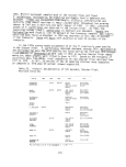 Frank Pine, then a graduate student at The Johns Hopkins University,
surveyed various areas in the Chester River in the 1970s. With Robert Munro,
Pine surveyed Eastern Neck Island in 1970 and observed extensive beds of
Najas, Ruppia, P_. pectinatus and Zannichellia along the western shore. Pockets
of the same species were noted on the eastern side of the island. By the spring
of 1972, the large western beds were reduced to virtually nothing while vegeta-
tion pockets remained on the eastern side. Excessive turbidity was noted at
the time.
Area 25. Love and Kent Points
The Chesapeake Bay shore between Kent and Love Points was surveyed in
1961 by Milfoil Survey teams (see Table 53). One transect was run perpendicular
to the Bay shore line as part of the Benthic Survey in 1961. Both surveys docu-
mented a total of four species. By the 1969 Vegetation Survey, three species
were documented with Ruppia dominant. In 1974, Ruppia alone was documented off
Chews Point, north of Bloody Point, by the MBHRL Survey.
Table 53. Historic documentation of SAV by decades, Love and Kent
Points, Maryland (Area 25)
Species 1960 1970
Potamogeton 1961(B)(M)
perfoliatus 1969(V)
Ruppia 1961(B)(M) 1974(MB)
maritima 1969(V)
Zostera 1961(M)
marina 1969(V)
Vallisneria 1961(M)
americana
Area 26. Smith Island
Vegetation around Smith Island has been predominantly Zostera and Ruppia
(see Table 54). Both species were documented by the Vegetation Survey in 1967
at the same percentage of transects though by the initation of the MBHRL Survey
in 1971, Ruppia seemed to be more common than Zostera. Since that time, Zostera
has declined sharply, based on percentage occurrence. Ruppia has also declined
but showed a recovery in 1976. P_. pectinatus was observed in both 1972 and 1973
in "more than trace" amounts. Subsequent MBHRL surveys in 1974 and 1976 have
not documented any further P. pectinatus.
179
image:
Frank Pine, then a graduate student at The Johns Hopkins University,
surveyed various areas in the Chester River in the 1970s. With Robert Munro,
Pine surveyed Eastern Neck Island in 1970 and observed extensive beds of
Najas, Ruppia, P_. pectinatus and Zannichellia along the western shore. Pockets
of the same species were noted on the eastern side of the island. By the spring
of 1972, the large western beds were reduced to virtually nothing while vegeta-
tion pockets remained on the eastern side. Excessive turbidity was noted at
the time.
Area 25. Love and Kent Points
The Chesapeake Bay shore between Kent and Love Points was surveyed in
1961 by Milfoil Survey teams (see Table 53). One transect was run perpendicular
to the Bay shore line as part of the Benthic Survey in 1961. Both surveys docu-
mented a total of four species. By the 1969 Vegetation Survey, three species
were documented with Ruppia dominant. In 1974, Ruppia alone was documented off
Chews Point, north of Bloody Point, by the MBHRL Survey.
Table 53. Historic documentation of SAV by decades, Love and Kent
Points, Maryland (Area 25)
Species 1960 1970
Potamogeton 1961(B)(M)
perfoliatus 1969(V)
Ruppia 1961(B)(M) 1974(MB)
maritima 1969(V)
Zostera 1961(M)
marina 1969(V)
Vallisneria 1961(M)
americana
Area 26. Smith Island
Vegetation around Smith Island has been predominantly Zostera and Ruppia
(see Table 54). Both species were documented by the Vegetation Survey in 1967
at the same percentage of transects though by the initation of the MBHRL Survey
in 1971, Ruppia seemed to be more common than Zostera. Since that time, Zostera
has declined sharply, based on percentage occurrence. Ruppia has also declined
but showed a recovery in 1976. P_. pectinatus was observed in both 1972 and 1973
in "more than trace" amounts. Subsequent MBHRL surveys in 1974 and 1976 have
not documented any further P. pectinatus.
179
image:
 Table 54. Historic documentation of SAV by decades, Smith Island,
Maryland (Area 26)
Species
1960
1970
Potamogeton
pectin at us_
Ruppia
maritima
Zostera
marina
1967(V)
1967(V)
1972-1973(MB)
1971-1976(MB)
1971-1972(MB)
1975-1976(MB)
Area 29. Upper Potomac River
Francis Uhler, MBHRL, is often quoted concerning his report of seeing
ducks feeding pondweeds, Na.ias and Vail isneria, near the 14th Street Bridge
in the early 1930s (see Table 55). Stewart (1962) reported finding
P_. pectinatus along with Najas and Vail isneria in the 1950s (date not specified)
In 1952, Bartsch (1954) surveyed the upper Potomac River and determined that
vegetation was essentially nonexistent. Then, from 1958 until its dramatic
disappearance around 1965, Myriophyllum created nuisance conditions in the
upper Potomac.
Table 55. Historic documentation of SAV by decades, Upper Potomac
River, Maryland and Virginia, (Area 29)
Species
Potamogeton
Ruppia
maritima
Ifynophyl 1 urn
spicatum
P.. pectinatus
Vail isneria
americana
El odea
canedensis
Najas sp.
1890-1900
1877(H)
1884,1898(H)
1889(H)
1875(H)
1884,1895(H)
1900
1906(H)
1903(H)
1903(H)
1906(H)
1908(H)
1909(H)
1903(H)
1903(H)
1910 1920
1914(H) 1922(H)
1915(H)
1915(H)
191S(H)
1914(H) 1925(H)
1915(H)
1914(H)
1918(H)
1929(H)
1930 1940
1930(H)
1933(H)
1935(H)
1933(H)
1930s (U)
1935(H) 1941(H)
1944(H)
1933(H)
1934(H)
1939(H)
1930s (U)
1950
1951(H)
1957(H)
1952(H)
1950s (RS)
1950s(RS)
1950(H)
1951(H)
1950s (RS)
1960 1970
1963(H)
1969(H)
1977(EC)
1972(H)
Ceratophyl1um
demersum
1881,1895(H) 1903(H)
1915(H)
1918(H)
1935(H)
1936(H)
1944(H)
180
image:
Table 54. Historic documentation of SAV by decades, Smith Island,
Maryland (Area 26)
Species
1960
1970
Potamogeton
pectin at us_
Ruppia
maritima
Zostera
marina
1967(V)
1967(V)
1972-1973(MB)
1971-1976(MB)
1971-1972(MB)
1975-1976(MB)
Area 29. Upper Potomac River
Francis Uhler, MBHRL, is often quoted concerning his report of seeing
ducks feeding pondweeds, Na.ias and Vail isneria, near the 14th Street Bridge
in the early 1930s (see Table 55). Stewart (1962) reported finding
P_. pectinatus along with Najas and Vail isneria in the 1950s (date not specified)
In 1952, Bartsch (1954) surveyed the upper Potomac River and determined that
vegetation was essentially nonexistent. Then, from 1958 until its dramatic
disappearance around 1965, Myriophyllum created nuisance conditions in the
upper Potomac.
Table 55. Historic documentation of SAV by decades, Upper Potomac
River, Maryland and Virginia, (Area 29)
Species
Potamogeton
Ruppia
maritima
Ifynophyl 1 urn
spicatum
P.. pectinatus
Vail isneria
americana
El odea
canedensis
Najas sp.
1890-1900
1877(H)
1884,1898(H)
1889(H)
1875(H)
1884,1895(H)
1900
1906(H)
1903(H)
1903(H)
1906(H)
1908(H)
1909(H)
1903(H)
1903(H)
1910 1920
1914(H) 1922(H)
1915(H)
1915(H)
191S(H)
1914(H) 1925(H)
1915(H)
1914(H)
1918(H)
1929(H)
1930 1940
1930(H)
1933(H)
1935(H)
1933(H)
1930s (U)
1935(H) 1941(H)
1944(H)
1933(H)
1934(H)
1939(H)
1930s (U)
1950
1951(H)
1957(H)
1952(H)
1950s (RS)
1950s(RS)
1950(H)
1951(H)
1950s (RS)
1960 1970
1963(H)
1969(H)
1977(EC)
1972(H)
Ceratophyl1um
demersum
1881,1895(H) 1903(H)
1915(H)
1918(H)
1935(H)
1936(H)
1944(H)
180
image:
 MBHRL sampled the upper Potomac in 1972 but found no SAV. Based on the
lack of vegetation, sampling of the entire river was dropped from the MBHRL
Survey until 1977. Sampling of the same stations again documented no vegetation
during the summer of 1977.
Ecological Analysts (Towson, Maryland) is presently studying Piscataway
Creek for the Washington Suburban Sanitary Commission. Field personnel
noted in 1977 moderate sized beds of healthy Elodea canadensis and patchy but
healthy beds of Potamogeton crispus in creek bottoms just south of the mouth
of Piscataway Creek in the Potomac River (Pine, personal communication).
Area 30. Upper Middle Potomac River
Port Tobacco River was surveyed from 1960 to 1971 for the Milfoil Survey.
In 1969, with the exception of Goose Bay, the river was extremely turbid with
only traces of Ruppia, Myriophyllum and P_. perfoliatus. The water was clear in
Goose Bay and abundaBt with Myriophyllum. By 1970, an increase in SAV was
noted throughout the lower half of Port Tobacco River, principally Vallisneria,
Myriophyllum, P. perfoliatus and Ruppia. In 1971, sparse SAV growth extended
north to the upper marina area (see Table 56).
Table 56. Historic documentation of SAV by decades, Upper Middle Potomac
River, Maryland and Virginia
Species
Najas spp.
Ceratophyllum
demersum
1910
1920
1930
1940
1950
1960
1935(H)
1970
Potamogeton 1915(H) 1921(H) 1936(H) 1945(H) 1954(H) 1960,1965(M)
perfoliatus 1938(H) 1969(M)
Ruppid 1915(H) 1943(H) 1969(M)
maritima
Myriophyllum
spicatum
P. pectinatus 1934
Vallisneria 1927(U) 1933
americana 1934
Elodea
canadensis
1952(H) 1960,1965(M)
1969(M)(H)
H) 1969(M)
H) 1946(H)
H)
1969(M)
1970-1971(M)
1972,1977(MB)
1970-1971(M)
1972(MB)
1970-1971(M)
1972,1977(HB)
1970-1971(M)
1970-1971{M)
1972,1977(MB)
1977(MB)
1977(MB)
Nanjemoy Creek water was cloudy throughout 1969. Prior to the heavy rains
in July, scattered Myriophyllum and traces of P_. pectinatus were observed.
Water in the creek remained turbid throughout 1970 and 1971 and no SAV was
documented. In 1972, MBHRL sampled the Nanjemoy Creek and noted a pocket of
Vallisneria off Blossom Point at the mouth of the creek plus some Myriophyllum
further up on the western shore. Other than a pocket of Vallisneria off Taylor
Neck at Riverside anfl a trace of the same species across the river from Quantico,
no other vegetation was documented from Port Tobacco to Quantico. Sampling was
181
image:
MBHRL sampled the upper Potomac in 1972 but found no SAV. Based on the
lack of vegetation, sampling of the entire river was dropped from the MBHRL
Survey until 1977. Sampling of the same stations again documented no vegetation
during the summer of 1977.
Ecological Analysts (Towson, Maryland) is presently studying Piscataway
Creek for the Washington Suburban Sanitary Commission. Field personnel
noted in 1977 moderate sized beds of healthy Elodea canadensis and patchy but
healthy beds of Potamogeton crispus in creek bottoms just south of the mouth
of Piscataway Creek in the Potomac River (Pine, personal communication).
Area 30. Upper Middle Potomac River
Port Tobacco River was surveyed from 1960 to 1971 for the Milfoil Survey.
In 1969, with the exception of Goose Bay, the river was extremely turbid with
only traces of Ruppia, Myriophyllum and P_. perfoliatus. The water was clear in
Goose Bay and abundaBt with Myriophyllum. By 1970, an increase in SAV was
noted throughout the lower half of Port Tobacco River, principally Vallisneria,
Myriophyllum, P. perfoliatus and Ruppia. In 1971, sparse SAV growth extended
north to the upper marina area (see Table 56).
Table 56. Historic documentation of SAV by decades, Upper Middle Potomac
River, Maryland and Virginia
Species
Najas spp.
Ceratophyllum
demersum
1910
1920
1930
1940
1950
1960
1935(H)
1970
Potamogeton 1915(H) 1921(H) 1936(H) 1945(H) 1954(H) 1960,1965(M)
perfoliatus 1938(H) 1969(M)
Ruppid 1915(H) 1943(H) 1969(M)
maritima
Myriophyllum
spicatum
P. pectinatus 1934
Vallisneria 1927(U) 1933
americana 1934
Elodea
canadensis
1952(H) 1960,1965(M)
1969(M)(H)
H) 1969(M)
H) 1946(H)
H)
1969(M)
1970-1971(M)
1972,1977(MB)
1970-1971(M)
1972(MB)
1970-1971(M)
1972,1977(HB)
1970-1971(M)
1970-1971{M)
1972,1977(MB)
1977(MB)
1977(MB)
Nanjemoy Creek water was cloudy throughout 1969. Prior to the heavy rains
in July, scattered Myriophyllum and traces of P_. pectinatus were observed.
Water in the creek remained turbid throughout 1970 and 1971 and no SAV was
documented. In 1972, MBHRL sampled the Nanjemoy Creek and noted a pocket of
Vallisneria off Blossom Point at the mouth of the creek plus some Myriophyllum
further up on the western shore. Other than a pocket of Vallisneria off Taylor
Neck at Riverside anfl a trace of the same species across the river from Quantico,
no other vegetation was documented from Port Tobacco to Quantico. Sampling was
181
image:
 not conducted by MBHRL from 1973 through 1976, but was resumed in 1977. Haranris
(1977) surveyed the Potomac River for the MBHRL Survey and found that vegetation
appeared to be concentrated within a 46 km area extending from Sandy Point (just
south of Quantico on the Maryland shore) downstream to lower Cedar Point (just
south of the 301 bridge). The majority of this river stretch is in Area 30.
Haramis found lush growths of Vallisneria in Goose Bay and Port Tobacco River
and _P. perfoliatus and scattered Myriophyllum sp., C_. demersum, E_. canadensis,
and P_. pectinatus throughout the 46 km area. It is within this portion of the
Potomac River that the fresh and salt waters mix.
Area 31. Lower Middle Potomac River
The Milfoil Survey teams observed abundant P_. perfoliatus and P_. pectinatus
in the Breton and St. Clements Bays area in November of 1961. Myriophy'i'lum was
found locally abundant in several of the feeder creeks and Ruppia and Zostera
were determined to be generally rare (see Table 57).
The Wicomico River system was sampled by Rawls in August, 1965. Myriophyllum
was found in abundance in many of the creeks and bays. P_. perfoliatus was
abundant in St. Catherine Sound, Chaptico Bay and several creeks. Ruppia was
observed occasionally and Najas was found in Dolly Boarman's Creek.
In August, 1967, Chaptico Bay and the Wicomico were found by Rawls to be
quite turbid. Najas was abundant in Chaptico Bay, Ruppia occasional and IP.
perfoliatus common. The abundant Najas found in Dolly Boarman's Creek in 1965
was listed as rare to occasional near the mouth of the creek and occasional
inside the creek. In September, 1968, Chaptico Bay was sampled again and Ruppia,
Najas and P_. perfoliatus were documented as occasional to abundant. Approxi-
mately 25 to 30 ha of Myriophyllum were noted. In a letter to John Steenis,
dated September 25, 1968, Rawls related the status of Myriophyllum in 1968 to
the explosive growth in the late 1950s and early 1960s.
Water in the Wicomico by 1970 and 1971 was progressively more turbid up-
stream probably due to stream channelization that was in progress at Gilbert
Swamp. SAV growth was observed to be scattered with one pocket remaining at
the mouth of Chaptico Bay in the Bassfold embayment. Currioman Bay and Nomini
Creek were sampled from 1968 to 1971 as part of the Milfoil Survey but the
waters were determined to be too turbid for extensive SAV growth. Limited
growth of Ruppia and Myriophyllum plus traces of £_. perfoliatus were documented.
In 1972, MBHRL found a trace of Zannichellia up Nomini Creek.
In the Lower Machodoc and Glebe Creek area, no SAV was documented. Glebe
Creek was observed to be very turbid from 1969 to 1971 due to extensive marina,
suburban and recreational development along the shoreline. MBHRL summer
sampling in 1972 documented a bed of Vallisneria just off Persimmon Point.
Later, in 1976 and 1977, Uhler reported seeing sparse beds of Vallisneria at
the same location. MBHRL did not sample the Potomac River after 1972 until
1977 when Haramis (1977) reported having found an extensive bed of £. perfoliatus
and R. maritima on the southern shore of the 301 bridge.
182
image:
not conducted by MBHRL from 1973 through 1976, but was resumed in 1977. Haranris
(1977) surveyed the Potomac River for the MBHRL Survey and found that vegetation
appeared to be concentrated within a 46 km area extending from Sandy Point (just
south of Quantico on the Maryland shore) downstream to lower Cedar Point (just
south of the 301 bridge). The majority of this river stretch is in Area 30.
Haramis found lush growths of Vallisneria in Goose Bay and Port Tobacco River
and _P. perfoliatus and scattered Myriophyllum sp., C_. demersum, E_. canadensis,
and P_. pectinatus throughout the 46 km area. It is within this portion of the
Potomac River that the fresh and salt waters mix.
Area 31. Lower Middle Potomac River
The Milfoil Survey teams observed abundant P_. perfoliatus and P_. pectinatus
in the Breton and St. Clements Bays area in November of 1961. Myriophy'i'lum was
found locally abundant in several of the feeder creeks and Ruppia and Zostera
were determined to be generally rare (see Table 57).
The Wicomico River system was sampled by Rawls in August, 1965. Myriophyllum
was found in abundance in many of the creeks and bays. P_. perfoliatus was
abundant in St. Catherine Sound, Chaptico Bay and several creeks. Ruppia was
observed occasionally and Najas was found in Dolly Boarman's Creek.
In August, 1967, Chaptico Bay and the Wicomico were found by Rawls to be
quite turbid. Najas was abundant in Chaptico Bay, Ruppia occasional and IP.
perfoliatus common. The abundant Najas found in Dolly Boarman's Creek in 1965
was listed as rare to occasional near the mouth of the creek and occasional
inside the creek. In September, 1968, Chaptico Bay was sampled again and Ruppia,
Najas and P_. perfoliatus were documented as occasional to abundant. Approxi-
mately 25 to 30 ha of Myriophyllum were noted. In a letter to John Steenis,
dated September 25, 1968, Rawls related the status of Myriophyllum in 1968 to
the explosive growth in the late 1950s and early 1960s.
Water in the Wicomico by 1970 and 1971 was progressively more turbid up-
stream probably due to stream channelization that was in progress at Gilbert
Swamp. SAV growth was observed to be scattered with one pocket remaining at
the mouth of Chaptico Bay in the Bassfold embayment. Currioman Bay and Nomini
Creek were sampled from 1968 to 1971 as part of the Milfoil Survey but the
waters were determined to be too turbid for extensive SAV growth. Limited
growth of Ruppia and Myriophyllum plus traces of £_. perfoliatus were documented.
In 1972, MBHRL found a trace of Zannichellia up Nomini Creek.
In the Lower Machodoc and Glebe Creek area, no SAV was documented. Glebe
Creek was observed to be very turbid from 1969 to 1971 due to extensive marina,
suburban and recreational development along the shoreline. MBHRL summer
sampling in 1972 documented a bed of Vallisneria just off Persimmon Point.
Later, in 1976 and 1977, Uhler reported seeing sparse beds of Vallisneria at
the same location. MBHRL did not sample the Potomac River after 1972 until
1977 when Haramis (1977) reported having found an extensive bed of £. perfoliatus
and R. maritima on the southern shore of the 301 bridge.
182
image:
 Table 57. Historic documentation of SAV by decades, Lower Middle
Potomac River, Maryland and Virginia (Area 31)
Species
Potamogeton
perfoliatus
Ruppia
maritima
Myriophyllum
spicatum
Zostera
marina
P. pectinatus
Zannichellia
palustris
Vallisneria
americana
Elodea
canadensis
Najas spp.
1930 1940 1960
1961,1965(M)
1967,1969(M)
1966,1968(H)
1933(H) 1961,1965(M)
1935(H) 1967.1968CM)
1966,1968(H)
1960,1963(H)
1961,1965(M)
1967-1969(M)
1966(H)
1961,1965(M)
1968(M)
1933(H) 1961,1969(M)
1936(H)
1933(H)
1946(H) 1965(M)
1967-1968(M)
1970
1970(H)
1970-1971(M)
1972,1977(MB)
1977(MB)
1970(H)
1970-1971(M)
1972(MB)
1970-1971(M)
1972(MB)
1970,1971(M)
1972{MB)
1976-1977(U)
1970-1971(M)
1972(MB)
1970-1971(M)
1972(MB)
Area 32. Lower Potomac River
The Milfoil Survey in 1961 documented virtually no SAV along the northern
shore of the Potomac River from Point Lookout to the western point of the St.
Mary's River (see Table 58).
Table 58. Historic documentation of SAV by decades, Lower Potomac
River, Maryland and Virginia (Area 32)
Species
1890
1920
1960
1970
Potamogeton
perfoliatus
Ruppia
maritir
ma
MyriophyTlum
spicatum
Zostera
marina
P. pectinatus
1928(H) 1961(M)
1894(H) 1928(H) 1961-1965(M)
1961(M)
1961,1963-1965(M)
1969(H)
1961,1963(M)
1973(H)
183
image:
Table 57. Historic documentation of SAV by decades, Lower Middle
Potomac River, Maryland and Virginia (Area 31)
Species
Potamogeton
perfoliatus
Ruppia
maritima
Myriophyllum
spicatum
Zostera
marina
P. pectinatus
Zannichellia
palustris
Vallisneria
americana
Elodea
canadensis
Najas spp.
1930 1940 1960
1961,1965(M)
1967,1969(M)
1966,1968(H)
1933(H) 1961,1965(M)
1935(H) 1967.1968CM)
1966,1968(H)
1960,1963(H)
1961,1965(M)
1967-1969(M)
1966(H)
1961,1965(M)
1968(M)
1933(H) 1961,1969(M)
1936(H)
1933(H)
1946(H) 1965(M)
1967-1968(M)
1970
1970(H)
1970-1971(M)
1972,1977(MB)
1977(MB)
1970(H)
1970-1971(M)
1972(MB)
1970-1971(M)
1972(MB)
1970,1971(M)
1972{MB)
1976-1977(U)
1970-1971(M)
1972(MB)
1970-1971(M)
1972(MB)
Area 32. Lower Potomac River
The Milfoil Survey in 1961 documented virtually no SAV along the northern
shore of the Potomac River from Point Lookout to the western point of the St.
Mary's River (see Table 58).
Table 58. Historic documentation of SAV by decades, Lower Potomac
River, Maryland and Virginia (Area 32)
Species
1890
1920
1960
1970
Potamogeton
perfoliatus
Ruppia
maritir
ma
MyriophyTlum
spicatum
Zostera
marina
P. pectinatus
1928(H) 1961(M)
1894(H) 1928(H) 1961-1965(M)
1961(M)
1961,1963-1965(M)
1969(H)
1961,1963(M)
1973(H)
183
image:
 St. George Creek, by contrast, was found to contain abundant growths of
IP. perfoliatus, £_. pectinatus and Ruppla. Herring Creek was abundant with
P.. perfoliatus, Ruppia and Myriophyllum. Big Ducks Creek, just to the north,
contained abundant Myriophyllum and occasional Ruppia. Blake Creek was also
documented as being abundant with Myriophyluum.
Both shores were sampled in 1972 by MBHRL but no vegetation was found.
When the MBHRL Survey was resumed in 1977, vegetation was listed as very sparse
(Haramis 1977).
Rappahannock River, Virginia
The only documentation readily available for the Rappahannock River is
for the 1970s. Orth studied aerial surveys of the river in order to map SAV
beds but it was not possible to separate Zostera_ marina and Ruppia martima on
on the photographs. It is probable that both species were in the river. Priest
surveyed the river in the summer of 1977 and found the two species already men-
tioned along with Z. palustris and an unknown species of Potamogeton (see Table
59).
Table 59. Historic documentation of SAV by decades, Rappahannock River,
Virginia
Species 1970
Ruppia 1971-1974(0)a
maritima 1977(WP)
Zostera 1971-1974(0)a
marina 1973(0)a
Zannichellia 1977(WP)
palustris
Potamogeton 1977(WP)
(? epihydrus)
Aerial survey by Orth did not differentiate between
Zostera and Ruppia
Piankatank River, Virginia
Documentation information for the Piankatank River is available only for
1971 through 1977. Orth documented Zostera and Ruppia and Priest found two
beds of Zannichellia (see Table 60). Data is insufficient for conclusions
regarding population or density changes.
184
image:
St. George Creek, by contrast, was found to contain abundant growths of
IP. perfoliatus, £_. pectinatus and Ruppla. Herring Creek was abundant with
P.. perfoliatus, Ruppia and Myriophyllum. Big Ducks Creek, just to the north,
contained abundant Myriophyllum and occasional Ruppia. Blake Creek was also
documented as being abundant with Myriophyluum.
Both shores were sampled in 1972 by MBHRL but no vegetation was found.
When the MBHRL Survey was resumed in 1977, vegetation was listed as very sparse
(Haramis 1977).
Rappahannock River, Virginia
The only documentation readily available for the Rappahannock River is
for the 1970s. Orth studied aerial surveys of the river in order to map SAV
beds but it was not possible to separate Zostera_ marina and Ruppia martima on
on the photographs. It is probable that both species were in the river. Priest
surveyed the river in the summer of 1977 and found the two species already men-
tioned along with Z. palustris and an unknown species of Potamogeton (see Table
59).
Table 59. Historic documentation of SAV by decades, Rappahannock River,
Virginia
Species 1970
Ruppia 1971-1974(0)a
maritima 1977(WP)
Zostera 1971-1974(0)a
marina 1973(0)a
Zannichellia 1977(WP)
palustris
Potamogeton 1977(WP)
(? epihydrus)
Aerial survey by Orth did not differentiate between
Zostera and Ruppia
Piankatank River, Virginia
Documentation information for the Piankatank River is available only for
1971 through 1977. Orth documented Zostera and Ruppia and Priest found two
beds of Zannichellia (see Table 60). Data is insufficient for conclusions
regarding population or density changes.
184
image:
 Table 60. Historic documentation of SAV by decades, Piankatank River,
Virginia
Species 1970
Zostera 1973(0)
marina 1971, 1974(0)a
Ruppia 1971, 1974(0)a
maritima
Zannichellia 1977(WP)
pulustris
Aerial survey by Orth did not differentiate between Zostera
and Ruppia
Mobjack Bay, Virginia
Ruppia maritima and Zostera marina
are the only two species of SAV that have been documented in Mobjack Bay.
Zostera was found in 1969 and also by two survey crews in the 1970s. Ruppia
was sited by Orth and also by the MBHRL Survey personnel during their one-and-
only survey of Mobjack Bay (see Table 61).
Table 61. Historic documentation of SAV by decades, Mobjack Bay,
Virginia
Species 1960 1970
Ruppia 1969 (H) 1972(MB)
maritima 1971,19/4(0)a
Zostera 1972(MB)
marina 1971,1974(0)a
aerial survey by Orth did not differentiate between Zostera
and Ruppia
185
image:
Table 60. Historic documentation of SAV by decades, Piankatank River,
Virginia
Species 1970
Zostera 1973(0)
marina 1971, 1974(0)a
Ruppia 1971, 1974(0)a
maritima
Zannichellia 1977(WP)
pulustris
Aerial survey by Orth did not differentiate between Zostera
and Ruppia
Mobjack Bay, Virginia
Ruppia maritima and Zostera marina
are the only two species of SAV that have been documented in Mobjack Bay.
Zostera was found in 1969 and also by two survey crews in the 1970s. Ruppia
was sited by Orth and also by the MBHRL Survey personnel during their one-and-
only survey of Mobjack Bay (see Table 61).
Table 61. Historic documentation of SAV by decades, Mobjack Bay,
Virginia
Species 1960 1970
Ruppia 1969 (H) 1972(MB)
maritima 1971,19/4(0)a
Zostera 1972(MB)
marina 1971,1974(0)a
aerial survey by Orth did not differentiate between Zostera
and Ruppia
185
image:
 York River, Virginia
Historic documentation of aquatic vegetation in the York River spans six
decades. Zostera has been documented fairly steadily since the 1930s (see
Table 62). Vallisneria, El odea, Ruppia and 'P.pectinatus have each been
listed once. The lack of comprehensive survey work in Virginia waters pre-
cludes any conclusions based on these random sitings.
Table 62. Historic documentation of SAV by decades, York River, Virginia
Species
1920
1930
1950
1960
1970
Potamogeton
pectinatus
Ruppia
mantima
Zostera
marina
Vallisneria 1926(H)
americana
El odea
canadensis
1958(H)
1971,1974(0)a
1937(0) 1953(0) 1960(0) 1970,1973(0),
1963(0) 1971,1974(0)
1975,1977(0)
1958(H)
aAerial survey by Orth did not differentiate between Zostera and Ruppia
Tangier Island, Virginia
The MBHRL Survey team surveyed Tangier Sound once in the summer of 1972.
Ruppia was found to be occasionally abundant butmostoften was present in
trace amounts. Zostera appeared to be dominant and £_. pectinatus was found to
be abundant around Fishbone Island but was otherwise not present (see Table 63)
Table 63.
Virginia
Historic documentation of SAV by decade, Tangier Island,
Species
1970
Ruppia maritima
Potamogeton pectinatus
Zostera marina
1972 (MB)
1972 (MB)
1972 (MB)
186
image:
York River, Virginia
Historic documentation of aquatic vegetation in the York River spans six
decades. Zostera has been documented fairly steadily since the 1930s (see
Table 62). Vallisneria, El odea, Ruppia and 'P.pectinatus have each been
listed once. The lack of comprehensive survey work in Virginia waters pre-
cludes any conclusions based on these random sitings.
Table 62. Historic documentation of SAV by decades, York River, Virginia
Species
1920
1930
1950
1960
1970
Potamogeton
pectinatus
Ruppia
mantima
Zostera
marina
Vallisneria 1926(H)
americana
El odea
canadensis
1958(H)
1971,1974(0)a
1937(0) 1953(0) 1960(0) 1970,1973(0),
1963(0) 1971,1974(0)
1975,1977(0)
1958(H)
aAerial survey by Orth did not differentiate between Zostera and Ruppia
Tangier Island, Virginia
The MBHRL Survey team surveyed Tangier Sound once in the summer of 1972.
Ruppia was found to be occasionally abundant butmostoften was present in
trace amounts. Zostera appeared to be dominant and £_. pectinatus was found to
be abundant around Fishbone Island but was otherwise not present (see Table 63)
Table 63.
Virginia
Historic documentation of SAV by decade, Tangier Island,
Species
1970
Ruppia maritima
Potamogeton pectinatus
Zostera marina
1972 (MB)
1972 (MB)
1972 (MB)
186
image:
 Pocomoke Sound, Virginia
The Pocomoke Sound area was covered in 1972 by an MBHRL Survey crew.
As would be expected of such a high saline area, Ruppia and Zostera were
the only SAV species found. Zostera was the dominant species while Ruppia
was found mainly in only trace amounts (see Table 64).
Table 64. Historic documentation of SAV by decades, Pocomoke Sound,
Virginia
Species 1970
Ruppia 1972 (MB)
maritima
Zostera 1972 (MB)
marina
SUMMARY OF CONCLUSIONS
Submerged aquatic vegetation in the Chesapeake Bay has changed in species
density, diversity and distribution over the past forty years (Renn 1937;
Rawls 1964; Sculthorpe 1967; Lind and Cottam 1939; Elser, 1969; Holm et al.
1969; Bayley et al. in press). Some native species have disappeared, domina-
nance patterns have changed, drastic fluctuations in yearly SAV populations
have been noted and seasonal patterns of growth, decline and reproduction
have shifted.
Based on the lack of historic documented evidence for SAV in the Virginia
portion of the Cheapeake Bay, conclusions based on data presented in this
chapter pertain to Maryland Chesapeake Bay waters. Information for Virginia
SAV is primarily limited to the work of Orth and Priest, working independently
at the Virginia Institute of Marine Science.
During the first part of this century, the upper Potomac and Anacostia
River estuaries were considered healthy ecosystems. But since that time, the
flora and fauna of these upper tidal estuaries have diminished in diversity and
density. In other parts of the Cheapeake Bay estuary, similar declines have
been documented. Seven species of SAV were documented in the Sassafras River
in the 1960s but only two have been found in the 1970s. The Susquehanna Flats
that have served as a noted duck feeding ground no longer support the lush
growths of SAV that have been documented over the past century. The Patuxent
River supported at least eight species cf SAV in the 1960s but only four species
•ave been found in the 1970s. Around Curtis and Cove Points, four species
lave been documented since 1930 but MBHRL Survey teams have found nothing from
i971 to 1976.
187
image:
Pocomoke Sound, Virginia
The Pocomoke Sound area was covered in 1972 by an MBHRL Survey crew.
As would be expected of such a high saline area, Ruppia and Zostera were
the only SAV species found. Zostera was the dominant species while Ruppia
was found mainly in only trace amounts (see Table 64).
Table 64. Historic documentation of SAV by decades, Pocomoke Sound,
Virginia
Species 1970
Ruppia 1972 (MB)
maritima
Zostera 1972 (MB)
marina
SUMMARY OF CONCLUSIONS
Submerged aquatic vegetation in the Chesapeake Bay has changed in species
density, diversity and distribution over the past forty years (Renn 1937;
Rawls 1964; Sculthorpe 1967; Lind and Cottam 1939; Elser, 1969; Holm et al.
1969; Bayley et al. in press). Some native species have disappeared, domina-
nance patterns have changed, drastic fluctuations in yearly SAV populations
have been noted and seasonal patterns of growth, decline and reproduction
have shifted.
Based on the lack of historic documented evidence for SAV in the Virginia
portion of the Cheapeake Bay, conclusions based on data presented in this
chapter pertain to Maryland Chesapeake Bay waters. Information for Virginia
SAV is primarily limited to the work of Orth and Priest, working independently
at the Virginia Institute of Marine Science.
During the first part of this century, the upper Potomac and Anacostia
River estuaries were considered healthy ecosystems. But since that time, the
flora and fauna of these upper tidal estuaries have diminished in diversity and
density. In other parts of the Cheapeake Bay estuary, similar declines have
been documented. Seven species of SAV were documented in the Sassafras River
in the 1960s but only two have been found in the 1970s. The Susquehanna Flats
that have served as a noted duck feeding ground no longer support the lush
growths of SAV that have been documented over the past century. The Patuxent
River supported at least eight species cf SAV in the 1960s but only four species
•ave been found in the 1970s. Around Curtis and Cove Points, four species
lave been documented since 1930 but MBHRL Survey teams have found nothing from
i971 to 1976.
187
image:
 Looking at the entire Maryland Bay, there is a general downward trend in
vegetation occurrence and abundance, especially from 1971 through 1976. But,
the losses appear to be random rather than predictable declines based on an
epicenter concept or a large scale natural disaster. When data for decreasing
species are combined for 1971 to 1976, there is no visible consistent trend of
loss from any one point. Unlike some situations, such as the shellfish
mortality in the Chester River in which increasing declines occurred down
river in a gradient pattern, the SAV survey pattern does not indicate a
strong point source mortality.
The basic questions which require consideration are whether Bay vegetation
is (1) experiencing a normal population fluctuation, (2) responding to pollu-
tion or other man-oriented impacts or (3) both.. The hypothesis of a normal
cycle situation requires historical documentation of similar events in the past.
But there is no documentation of such a significant portion of submerged flora
having been so negatively impacted for such a long period of time. Only two
species have been known for dramatic populations crashed in the past: Zostera
and Myriophyllum. In both cases, other Bay species were able to replace them
relatively quickly. This was a different system response than what has been
seen in the 1970s when all species seem to have been negatively affected.
The variety and degree of human impacts, including a wide range of known
or suspected pollutants, appear to be of greater relevance to recent declines
in rooted aquatics than a naturally occurring cycle event. However, the
hypothesis that the Bay is experiencing a cyclic phenomenon cannot be entirely
ruled out. For example, the Bay has not appeared to be as resilient in the
1970s to excessive storms as was evinced during the 1930s. Hurricane Agnes
seemed to have resulted in a greater negative impact of longer duration than
comparable storms of the 1930s. Slower regrowth after Agnes may have resulted
from negetive impacts incurred by the seagrass ecosystem due to man-oriented
impacts and pollutants. Historic analysis of the upper Potomac River and
Baltimore Harbor show once prolific vegetation areas now practically barren
of floral species, semmingly due to excessive nutrient and pollution levels.
Thus, if the Bay is experiencing a normal population fluctuation such a
hypothesis would require consideration of human impacts on such a cycle.
Historic documentation of sufficient intensity and coverage necessary
to support a cyclic phenomenon hypothesis is lacking. Therefore, those
environmental parameters that have been impacted by man's activities in and
around the Chesapeake Bay are discussed in the following chapter. Each para-
meter is discussed singly due to the mono-factorial nature of most experiments.
In that the environment is more realistically a multifactorial system, it is
likely that SAV declines have resulted from no single factor but from a
multitude of factors or synergisms.
188
image:
Looking at the entire Maryland Bay, there is a general downward trend in
vegetation occurrence and abundance, especially from 1971 through 1976. But,
the losses appear to be random rather than predictable declines based on an
epicenter concept or a large scale natural disaster. When data for decreasing
species are combined for 1971 to 1976, there is no visible consistent trend of
loss from any one point. Unlike some situations, such as the shellfish
mortality in the Chester River in which increasing declines occurred down
river in a gradient pattern, the SAV survey pattern does not indicate a
strong point source mortality.
The basic questions which require consideration are whether Bay vegetation
is (1) experiencing a normal population fluctuation, (2) responding to pollu-
tion or other man-oriented impacts or (3) both.. The hypothesis of a normal
cycle situation requires historical documentation of similar events in the past.
But there is no documentation of such a significant portion of submerged flora
having been so negatively impacted for such a long period of time. Only two
species have been known for dramatic populations crashed in the past: Zostera
and Myriophyllum. In both cases, other Bay species were able to replace them
relatively quickly. This was a different system response than what has been
seen in the 1970s when all species seem to have been negatively affected.
The variety and degree of human impacts, including a wide range of known
or suspected pollutants, appear to be of greater relevance to recent declines
in rooted aquatics than a naturally occurring cycle event. However, the
hypothesis that the Bay is experiencing a cyclic phenomenon cannot be entirely
ruled out. For example, the Bay has not appeared to be as resilient in the
1970s to excessive storms as was evinced during the 1930s. Hurricane Agnes
seemed to have resulted in a greater negative impact of longer duration than
comparable storms of the 1930s. Slower regrowth after Agnes may have resulted
from negetive impacts incurred by the seagrass ecosystem due to man-oriented
impacts and pollutants. Historic analysis of the upper Potomac River and
Baltimore Harbor show once prolific vegetation areas now practically barren
of floral species, semmingly due to excessive nutrient and pollution levels.
Thus, if the Bay is experiencing a normal population fluctuation such a
hypothesis would require consideration of human impacts on such a cycle.
Historic documentation of sufficient intensity and coverage necessary
to support a cyclic phenomenon hypothesis is lacking. Therefore, those
environmental parameters that have been impacted by man's activities in and
around the Chesapeake Bay are discussed in the following chapter. Each para-
meter is discussed singly due to the mono-factorial nature of most experiments.
In that the environment is more realistically a multifactorial system, it is
likely that SAV declines have resulted from no single factor but from a
multitude of factors or synergisms.
188
image:
 CHAPTER 4
ASSESSMENT OF ENVIRONMENTAL FACTORS
INTRODUCTION
There are various environmental and human related factors that affect the
establishment, growth and reproduction of submerged aquatic vegetation in the
Chesapeake Bay. Included among these are agrochemicals, salinity, turbidity,
light, bottom substrate, nutrients, fauna, epiphytes, pH, temperature, heavy
metals, petroleum products and water movement. Although there have been gradual
changes in many of the environmental factors over the years, others, especially
the human related factors, have changed more rapidly.
The dynamic nature of the Chesapeake Bay as a wind driven estuary naturally
results in gradual changes in such parameters as salinity, bottom substrate and
fauna. However, the changes that have resulted from increasing human impacts
have been much more rapid. Increasing human population in the Bay area has
affected land use patterns since 1900. Agricultural land use has decreased;
fertilizer, lime and herbicide usage has increased; cropping practices have
changed; wetlands have decreased in acreage by almost half. Rising population
has also resulted in an increase in water, electric, sewage and industrial de-
mands. In order to meet these demands, numerous water and sewage treatment
plants, hydro-electric and industrial manufacturing facilities have been estab-
lished in the Bay area. All of these facilities utilize the waters of the Bay
and subsequently impact the estuarine system.
In order to assess the causes for the apparent declines in SAV, the various
factors that have changed within the Bay area must be analyzed. This chapter
presents these factors and attempts to selectively consider each one in order
to determine the probable cause for Bay grass declines.
AGRO-CHEMICALS
Introduction
Land use patterns in Maryland and Virginia have changed drastically since
the turn of the century. For Maryland alone, total land area of wetlands and
agriculture has been halved since 1900 while forested land has increased slightly.
Of major interest to this document is the decrease in agricultural land use
(see Table 65) and associated changes in cropping practices. In order to
189
image:
CHAPTER 4
ASSESSMENT OF ENVIRONMENTAL FACTORS
INTRODUCTION
There are various environmental and human related factors that affect the
establishment, growth and reproduction of submerged aquatic vegetation in the
Chesapeake Bay. Included among these are agrochemicals, salinity, turbidity,
light, bottom substrate, nutrients, fauna, epiphytes, pH, temperature, heavy
metals, petroleum products and water movement. Although there have been gradual
changes in many of the environmental factors over the years, others, especially
the human related factors, have changed more rapidly.
The dynamic nature of the Chesapeake Bay as a wind driven estuary naturally
results in gradual changes in such parameters as salinity, bottom substrate and
fauna. However, the changes that have resulted from increasing human impacts
have been much more rapid. Increasing human population in the Bay area has
affected land use patterns since 1900. Agricultural land use has decreased;
fertilizer, lime and herbicide usage has increased; cropping practices have
changed; wetlands have decreased in acreage by almost half. Rising population
has also resulted in an increase in water, electric, sewage and industrial de-
mands. In order to meet these demands, numerous water and sewage treatment
plants, hydro-electric and industrial manufacturing facilities have been estab-
lished in the Bay area. All of these facilities utilize the waters of the Bay
and subsequently impact the estuarine system.
In order to assess the causes for the apparent declines in SAV, the various
factors that have changed within the Bay area must be analyzed. This chapter
presents these factors and attempts to selectively consider each one in order
to determine the probable cause for Bay grass declines.
AGRO-CHEMICALS
Introduction
Land use patterns in Maryland and Virginia have changed drastically since
the turn of the century. For Maryland alone, total land area of wetlands and
agriculture has been halved since 1900 while forested land has increased slightly.
Of major interest to this document is the decrease in agricultural land use
(see Table 65) and associated changes in cropping practices. In order to
189
image:
 Table 65 oa
1 850-1 974a
Year
1850
1860
1870
1880
1890
1900
1910
1920
1930
1940
1950
1959
1969
1974
Total farmland
Maryland
(hectares)
1,875,521
1,956,956
1,826,241
2,071,996
2,004,232
2,092,329
2,046,625
1,925,562
1,770,319
1,698,861
1,641,273
1,398,954
1,134,553
1,079,611
in Maryland and Virginia
Virginia
(hectares)
No information
No information
No information
No information
No information
No information
7,889,884
7,511,682
6,770,072
6,655,254
6,302,108
5,312,012
4,309,999
4,492,170
U.S. Department of Commerce 1974
Approximate land area in Maryland =
2,574,799 hectares
Approximate land area in Virginia=
10,428,180 hectares
190
image:
Table 65 oa
1 850-1 974a
Year
1850
1860
1870
1880
1890
1900
1910
1920
1930
1940
1950
1959
1969
1974
Total farmland
Maryland
(hectares)
1,875,521
1,956,956
1,826,241
2,071,996
2,004,232
2,092,329
2,046,625
1,925,562
1,770,319
1,698,861
1,641,273
1,398,954
1,134,553
1,079,611
in Maryland and Virginia
Virginia
(hectares)
No information
No information
No information
No information
No information
No information
7,889,884
7,511,682
6,770,072
6,655,254
6,302,108
5,312,012
4,309,999
4,492,170
U.S. Department of Commerce 1974
Approximate land area in Maryland =
2,574,799 hectares
Approximate land area in Virginia=
10,428,180 hectares
190
image:
 compensate for the decline in land available for agricultural use, more
efficient cropping methods have been developed. These changes have brought
about increased usage of fertilizers, limes and new selective and contact
herbicides.
No-till and minimum till cropping have become popular in the Bay area within
the past several decades due to economic and conservation requirements. Though
often referred to by other descriptive terms, these tillage techniques result
in the least possible disturbance of the soil in order to effect seed placement,
weed control and crop maturation (Shear 1965). Minimum soil displacement and
maximum plant ground cover resulting from these techniques aid in the control
of a varity of sound environmental practices: reduced wind and water erosion;
increased soil organic content; reduced soil moisture evaporation; and increased
infiltration of rainfall (Shear 1965; Bauemer and Bakermans 1972).
No-till and minimum till farming require the use of greater quantities of
herbicides than conventional farming techniques. The presence of herbicides
in agricultural runoff and the impact of herbicides to aquatic fauna and flora
have recently become an issue for environmental concern, especially in an
estuary such as the Cheapeake Bay where no-till has become popular. Increases
in herbicide pound usage regardless of the source, have been implicated in the
recent SAV declines of the 1970s. The role of no-till and minimum till farming
as a source of water and soil borne herbicides is unknown at the present time.
Despite the larger poundage rates that are necessitated with no-till farming
compared to conventional farming techniques, no-till farming appears to result
in reduced soil and water runoff. Since runoff is the major avenue for the
introduction of herbicides into surrounding waters , no-till farming could
possibly result in decreased amounts of herbicides reaching the aquatic environ-
ment. The extent to which erosion is decreased in relation to increases in
herbicide poundage available to runoff has yet to be determined.
Fertilizers and Lime
The use of chemical fertilizers and lime have long been recognized for
increasing crop yields. In Maryland, the tonnage of fertilizers used since
1935 has about doubled while lime usage has increased more than seven fold
(see Table 66). Fertilizers have been used with direct aquatic application
for the control of submerged plants. However, the possible impact to SAV of
fertilizer and lime runoff as yet remains largely unknown.
Walker (1959) conducted pond studies on the distribution of water soluble
fertilizer (N-P-K value of 16-20-0) applied at 22 to 38.5 kg/ha. Effective
control of sago pondweed and mu kgrass resulted from a toxic reaction to the
fertilizer as well as by shading from subsequent plankton blooms. Application
of 110 kg/ha of 0-46-0 or 220 kg/ha of 8-24-8 sometimes stimulated filamentous
algae growth. Of the three fertilizers studied, 0-46-0 and 8-24-8 did not
control the submerged aquatic plants as effectively as 16-20-0.
Using plastic pools, Ryan et al. (1972) conducted a study to determine the
effects of fertilization on the growth and mineral composition of three aquatic
plant species; Eurasian watermilfoil, elodea and heartleafed pondweed. A
191
image:
compensate for the decline in land available for agricultural use, more
efficient cropping methods have been developed. These changes have brought
about increased usage of fertilizers, limes and new selective and contact
herbicides.
No-till and minimum till cropping have become popular in the Bay area within
the past several decades due to economic and conservation requirements. Though
often referred to by other descriptive terms, these tillage techniques result
in the least possible disturbance of the soil in order to effect seed placement,
weed control and crop maturation (Shear 1965). Minimum soil displacement and
maximum plant ground cover resulting from these techniques aid in the control
of a varity of sound environmental practices: reduced wind and water erosion;
increased soil organic content; reduced soil moisture evaporation; and increased
infiltration of rainfall (Shear 1965; Bauemer and Bakermans 1972).
No-till and minimum till farming require the use of greater quantities of
herbicides than conventional farming techniques. The presence of herbicides
in agricultural runoff and the impact of herbicides to aquatic fauna and flora
have recently become an issue for environmental concern, especially in an
estuary such as the Cheapeake Bay where no-till has become popular. Increases
in herbicide pound usage regardless of the source, have been implicated in the
recent SAV declines of the 1970s. The role of no-till and minimum till farming
as a source of water and soil borne herbicides is unknown at the present time.
Despite the larger poundage rates that are necessitated with no-till farming
compared to conventional farming techniques, no-till farming appears to result
in reduced soil and water runoff. Since runoff is the major avenue for the
introduction of herbicides into surrounding waters , no-till farming could
possibly result in decreased amounts of herbicides reaching the aquatic environ-
ment. The extent to which erosion is decreased in relation to increases in
herbicide poundage available to runoff has yet to be determined.
Fertilizers and Lime
The use of chemical fertilizers and lime have long been recognized for
increasing crop yields. In Maryland, the tonnage of fertilizers used since
1935 has about doubled while lime usage has increased more than seven fold
(see Table 66). Fertilizers have been used with direct aquatic application
for the control of submerged plants. However, the possible impact to SAV of
fertilizer and lime runoff as yet remains largely unknown.
Walker (1959) conducted pond studies on the distribution of water soluble
fertilizer (N-P-K value of 16-20-0) applied at 22 to 38.5 kg/ha. Effective
control of sago pondweed and mu kgrass resulted from a toxic reaction to the
fertilizer as well as by shading from subsequent plankton blooms. Application
of 110 kg/ha of 0-46-0 or 220 kg/ha of 8-24-8 sometimes stimulated filamentous
algae growth. Of the three fertilizers studied, 0-46-0 and 8-24-8 did not
control the submerged aquatic plants as effectively as 16-20-0.
Using plastic pools, Ryan et al. (1972) conducted a study to determine the
effects of fertilization on the growth and mineral composition of three aquatic
plant species; Eurasian watermilfoil, elodea and heartleafed pondweed. A
191
image:
 Table 66 .
Maryland^
Year
1935
1936
1937
1938
1939
1940
1941
1942
1943
1944
1945
1946
1947
1948
1949
1950
1951
1952
1953
1954
1955
1956
1957
1958
1959
1960
1961
1962
1963
1964
1965
1966
1967
1968
1969
1970
1971
1972
1973
1974
1975
1976
Total fertilizer and
1935-19763
Fertil izer
(metric tons)
149,644
149,621
169,109
151,065
149,410
145,534
156,088
165,873
180,508
188,355
198,041
222,178
232,351
211,746
222,610
229,775
249,571
264,376
269,309
282,536
281,829
253,875
269,211
255,231
278,970
271,434
269,971
294,991
323,593
311,003
327,534
367,201
345,425
332,445
334,018
347,903
335,819
337,189
400,825
396,436
340,810
398,871
lime used in
Lime
(metric tons)
54,215
77,439
106,180
90,823
89,502
114,467
117,375
128,275
176,279
207,431
208,368
248,919
266,788
204,614
199,626
266,343
281 ,085
266,018
251,512
253,969
267,571
266,192
Not available
234,477
260,191
250,119
253,985
264,537
274,419
268,867
328,010
265,085
236,230
245,415
254,085
226,784
180,617
205,410
251,786
323,519
293,511
385,349
aMaryland Department of Agriculture 1963-1977
192
image:
Table 66 .
Maryland^
Year
1935
1936
1937
1938
1939
1940
1941
1942
1943
1944
1945
1946
1947
1948
1949
1950
1951
1952
1953
1954
1955
1956
1957
1958
1959
1960
1961
1962
1963
1964
1965
1966
1967
1968
1969
1970
1971
1972
1973
1974
1975
1976
Total fertilizer and
1935-19763
Fertil izer
(metric tons)
149,644
149,621
169,109
151,065
149,410
145,534
156,088
165,873
180,508
188,355
198,041
222,178
232,351
211,746
222,610
229,775
249,571
264,376
269,309
282,536
281,829
253,875
269,211
255,231
278,970
271,434
269,971
294,991
323,593
311,003
327,534
367,201
345,425
332,445
334,018
347,903
335,819
337,189
400,825
396,436
340,810
398,871
lime used in
Lime
(metric tons)
54,215
77,439
106,180
90,823
89,502
114,467
117,375
128,275
176,279
207,431
208,368
248,919
266,788
204,614
199,626
266,343
281 ,085
266,018
251,512
253,969
267,571
266,192
Not available
234,477
260,191
250,119
253,985
264,537
274,419
268,867
328,010
265,085
236,230
245,415
254,085
226,784
180,617
205,410
251,786
323,519
293,511
385,349
aMaryland Department of Agriculture 1963-1977
192
image:
 granular 8-8-2 fertilizer was used over two years and applied with three
different treatments: a single application of fertilizer at a rate of 672
kg/ha; six weekly applications of the same fertilizer at 112 kg/ha; and an
unfertilized control. The first year of the experiment the dry weight of
milfoil was significantly greater in the control pools than in pools receiving
the six weekly applications, due to competition from filamentous algae. Elodea
and heartleaf pondweed were not adversely affected since they were able to
grow through the mats of algae. During the second experimental year, both el odea
milfoil controls had significantly greater yields than either fertilization
treatments. Conversely, heartleaf pondweed had significantly greater yields
in the treated pools.
Though available literature does not reveal information concerning the im-
pact of fertilizers rich in runoff to SAV,Klausner et al. (1974) evaluated surface
runoff losses of nitrogen and inorganic phosphorus from moderately to somewhat
poorly drained soil as influenced by crop rotation, application rate and soil
management practices. For the two year study, they found soluble nitrogen and
inorganic phosphorus losses ranged from 0.39 to 29.23 and 0.04 to 0.49 kg/ha/year
respectively. Annual surface runoff of NhU-N was not significantly changed by
crop, fertilizer application rate or soil management techniques,but was related
to heavy fall application prior to a wet period. Inorganic phosphorus losses,
in comparison, were related more to application rate and soil management than
to time of application.
Increased levels of organic material in the water column,pi us nitrogen
and phosphorus, can give rise to eutrophic condi",ons where an aquatic ecosystem
is enriched beyond its assimilation and flushing capabilities. Under such en-
riched conditions, minute algae plants or phytoplankton tend to thrive causing
decreased light penetration. This shading effect from phytoplankton can be
sufficient to actively decrease submerged aquatic vegetation. Such a situation
has occurred in the Upper Potomac River where the water has been enriched far
beyond the assimilation and flushing capabilities of the river. Agricultural
fertilizers,whether from direct aquatic application or from indirect runoff
sources,can provide the necessary enrichment for eutrophication.
Stolp and Penner (1973) conducted an experiment which suggested the
possibility of increased phytotoxicity of herbicides when applied in conjunc-
tion with fertilizers. Though this study involved a terrestrial system, it is
possible that similar results would occur in an aquatic system. Such a
synergism should be considered in the investigation of herbicide and fertilizer
runoff impacts to submerged aquatic vegetation.
Table 67 lists available data on fertilizer usage for counties in the
Cheapeake Bay area. Of the eight Eastern Shore counties for which poundage
rates were available, all but one showed increased usage from 1970 to 1976.
Of the eight Western Shore counties, half showed increased fertilizer use.
The increased use of fertilizers around the Chesapeake Bay along with the
potential impacts of fertilizers in an aquatic system necessitate the inclusion
of fertilizers as a negative factor in an assessment of the effects of agro-
chemicals to the Bay.
193
image:
granular 8-8-2 fertilizer was used over two years and applied with three
different treatments: a single application of fertilizer at a rate of 672
kg/ha; six weekly applications of the same fertilizer at 112 kg/ha; and an
unfertilized control. The first year of the experiment the dry weight of
milfoil was significantly greater in the control pools than in pools receiving
the six weekly applications, due to competition from filamentous algae. Elodea
and heartleaf pondweed were not adversely affected since they were able to
grow through the mats of algae. During the second experimental year, both el odea
milfoil controls had significantly greater yields than either fertilization
treatments. Conversely, heartleaf pondweed had significantly greater yields
in the treated pools.
Though available literature does not reveal information concerning the im-
pact of fertilizers rich in runoff to SAV,Klausner et al. (1974) evaluated surface
runoff losses of nitrogen and inorganic phosphorus from moderately to somewhat
poorly drained soil as influenced by crop rotation, application rate and soil
management practices. For the two year study, they found soluble nitrogen and
inorganic phosphorus losses ranged from 0.39 to 29.23 and 0.04 to 0.49 kg/ha/year
respectively. Annual surface runoff of NhU-N was not significantly changed by
crop, fertilizer application rate or soil management techniques,but was related
to heavy fall application prior to a wet period. Inorganic phosphorus losses,
in comparison, were related more to application rate and soil management than
to time of application.
Increased levels of organic material in the water column,pi us nitrogen
and phosphorus, can give rise to eutrophic condi",ons where an aquatic ecosystem
is enriched beyond its assimilation and flushing capabilities. Under such en-
riched conditions, minute algae plants or phytoplankton tend to thrive causing
decreased light penetration. This shading effect from phytoplankton can be
sufficient to actively decrease submerged aquatic vegetation. Such a situation
has occurred in the Upper Potomac River where the water has been enriched far
beyond the assimilation and flushing capabilities of the river. Agricultural
fertilizers,whether from direct aquatic application or from indirect runoff
sources,can provide the necessary enrichment for eutrophication.
Stolp and Penner (1973) conducted an experiment which suggested the
possibility of increased phytotoxicity of herbicides when applied in conjunc-
tion with fertilizers. Though this study involved a terrestrial system, it is
possible that similar results would occur in an aquatic system. Such a
synergism should be considered in the investigation of herbicide and fertilizer
runoff impacts to submerged aquatic vegetation.
Table 67 lists available data on fertilizer usage for counties in the
Cheapeake Bay area. Of the eight Eastern Shore counties for which poundage
rates were available, all but one showed increased usage from 1970 to 1976.
Of the eight Western Shore counties, half showed increased fertilizer use.
The increased use of fertilizers around the Chesapeake Bay along with the
potential impacts of fertilizers in an aquatic system necessitate the inclusion
of fertilizers as a negative factor in an assessment of the effects of agro-
chemicals to the Bay.
193
image:
 to
en
i— i
•
en
,— i
s-
0
to
c.
i.
to
CD
CD
S-
-o
s-
o
Q.
CU
(C
(O
T3
o
S-
CO
CU
N
£Z
0
o
o
S-
03
E
oo
to
cu
J3
(O
1—
co to
c cu
O -r-
-L_) -t.-_*
c
•r- O
S- 0
CD HI
•*-• o
S- 00
cu
N E
i— CU
•r- 4->
•4-J to
S— (T3
CU LLJ
Li-
re
cu
cu
to
o
00
o
o
•r-
o
3
S-
cu
CO
CU
O
S-
0
Q
CD
C
S-
o
to
I—
E to
CU CU
£
•i—
CU
C_5
1^ O CM CO .— 1 i— 1 00
en oo O o en oo LO
i-< i-H
oo co r^- r< LO o CM
^t- «* in o co •* CM
1^ O 00 CM CM IO O
^t to ^r co en en o
co *s3~ en en co en co
LO r^ CM CM CO tO CO
i— i LO en CM to co co
CM O I — ^d" LO LO ^3"
CM CM i— t CM CM CM CM
CO
CU
tO CO ^" CM LO 1 — CO T-
oo CM «* «— i en o CM +->
to r^ en LO ^d~ en co c
^j- «d" en o o to *d~ o
CMCMCMCOCOCMCM O
cu
o
^j~ f—t LO en r^. CM r^ oo
LO CO CO CO f-- CM CO
cnr~-<^-i— itocoo c
to LO ^~ r^- o^ to c^ cu
i— 1 r— < i— It— It— It— 1 CM -t->
CO
CU
CM to LO «3~ r~~ en co
LO C3 to LO Cn ^^ CT^
en o CM en en ^ r^»
" -«^
CM CM CM CO CO CM CO
oo en r~- en •— i CM «^-
cn i— i to co to ^- oo
LO ^j- to co co LO o-
LO ^d- CM LO r-. 00 CM
CM CM CM CM CM CM CO
LO LO en ^3~ « — < » — i co
O LO tO CM ^3" CO 1 — .
r^. en co co oo LO CM
r— i o en «— i o en LO
i— 1 i— 1 r— ( r— 1 i— 1
O <— ( CM CO ^3- LO to S-
cn en en en en en en cu
i-H I— 1 i— It— 1 r— (i— 1 r— < >_
CO
•*— >-
-P
s-
cu
(O
to
cu
s_
-E
to
CD CU
o en
i- CU
Q_ C3
E
O
Ql
to
fB
3
'oi
cu -o
=1 s-
CD
o
_E
(O
CO
S-
o
(O
n:
en *^~ co to ^i" en «~~i
r— 4 r*^ en i^. CM ^j~ co
to LO r^ co «d- oo i— i
^^v . -^ _.
i— 1 r-H
CM r~~ i— i LO co co en
LO r^ o CM to co co
oo LO ^- LO r~- t—i i— i
*3" 'd" LO ^~ ^J~ CO ^j"
LO o en LO to en co
to «d~ oo to CM .— i i—<
CO CM to i— ( CD tO l^.
r~. to co to co LO LO
CM to ^J- co r— i co en
co o LO r^ i— t to o
CO 00 i— 1 O tO CO CO
o en «d- to LO co LO
t— 1 .— < CM CM <— 1 CM
*d~ *3~ ^d" co o r*^> ^J~
co LO f — . to o CM en
O CM O CO 'd- LO CO
CM i— 1 CO tO tO LO CM
r— 1 t— 1 i— 1 i-H I — 1 i— 1 CM
CO O IO t— 1 LO LO O
en CM co o CD to LO
to LO LO to r~- co *d-
r^ co co i— i co to CM
to r^ CM LO co co LO
co r^ to i— i co o to
*d~ co r^. co *d~ *d~ co
,— H r— 1 i— 1 .— I ! — 1 i— 1 .— I
1^ CO CM i— 1 <=J- -3- CO
CM co o r^ «^- to co
CO CM CO CO CM P^ CO
LO CM co LO to O r~-
r— 1 t— 1 t— 1 I— 1 i-H r— 1 r— 1
O r-H CM CO •* LO tO
en en en en en en en
i— I i— 1 i— 1 r— 1 r— 1 r— 1 t— 1
194
image:
to
en
i— i
•
en
,— i
s-
0
to
c.
i.
to
CD
CD
S-
-o
s-
o
Q.
CU
(C
(O
T3
o
S-
CO
CU
N
£Z
0
o
o
S-
03
E
oo
to
cu
J3
(O
1—
co to
c cu
O -r-
-L_) -t.-_*
c
•r- O
S- 0
CD HI
•*-• o
S- 00
cu
N E
i— CU
•r- 4->
•4-J to
S— (T3
CU LLJ
Li-
re
cu
cu
to
o
00
o
o
•r-
o
3
S-
cu
CO
CU
O
S-
0
Q
CD
C
S-
o
to
I—
E to
CU CU
£
•i—
CU
C_5
1^ O CM CO .— 1 i— 1 00
en oo O o en oo LO
i-< i-H
oo co r^- r< LO o CM
^t- «* in o co •* CM
1^ O 00 CM CM IO O
^t to ^r co en en o
co *s3~ en en co en co
LO r^ CM CM CO tO CO
i— i LO en CM to co co
CM O I — ^d" LO LO ^3"
CM CM i— t CM CM CM CM
CO
CU
tO CO ^" CM LO 1 — CO T-
oo CM «* «— i en o CM +->
to r^ en LO ^d~ en co c
^j- «d" en o o to *d~ o
CMCMCMCOCOCMCM O
cu
o
^j~ f—t LO en r^. CM r^ oo
LO CO CO CO f-- CM CO
cnr~-<^-i— itocoo c
to LO ^~ r^- o^ to c^ cu
i— 1 r— < i— It— It— It— 1 CM -t->
CO
CU
CM to LO «3~ r~~ en co
LO C3 to LO Cn ^^ CT^
en o CM en en ^ r^»
" -«^
CM CM CM CO CO CM CO
oo en r~- en •— i CM «^-
cn i— i to co to ^- oo
LO ^j- to co co LO o-
LO ^d- CM LO r-. 00 CM
CM CM CM CM CM CM CO
LO LO en ^3~ « — < » — i co
O LO tO CM ^3" CO 1 — .
r^. en co co oo LO CM
r— i o en «— i o en LO
i— 1 i— 1 r— ( r— 1 i— 1
O <— ( CM CO ^3- LO to S-
cn en en en en en en cu
i-H I— 1 i— It— 1 r— (i— 1 r— < >_
CO
•*— >-
-P
s-
cu
(O
to
cu
s_
-E
to
CD CU
o en
i- CU
Q_ C3
E
O
Ql
to
fB
3
'oi
cu -o
=1 s-
CD
o
_E
(O
CO
S-
o
(O
n:
en *^~ co to ^i" en «~~i
r— 4 r*^ en i^. CM ^j~ co
to LO r^ co «d- oo i— i
^^v . -^ _.
i— 1 r-H
CM r~~ i— i LO co co en
LO r^ o CM to co co
oo LO ^- LO r~- t—i i— i
*3" 'd" LO ^~ ^J~ CO ^j"
LO o en LO to en co
to «d~ oo to CM .— i i—<
CO CM to i— ( CD tO l^.
r~. to co to co LO LO
CM to ^J- co r— i co en
co o LO r^ i— t to o
CO 00 i— 1 O tO CO CO
o en «d- to LO co LO
t— 1 .— < CM CM <— 1 CM
*d~ *3~ ^d" co o r*^> ^J~
co LO f — . to o CM en
O CM O CO 'd- LO CO
CM i— 1 CO tO tO LO CM
r— 1 t— 1 i— 1 i-H I — 1 i— 1 CM
CO O IO t— 1 LO LO O
en CM co o CD to LO
to LO LO to r~- co *d-
r^ co co i— i co to CM
to r^ CM LO co co LO
co r^ to i— i co o to
*d~ co r^. co *d~ *d~ co
,— H r— 1 i— 1 .— I ! — 1 i— 1 .— I
1^ CO CM i— 1 <=J- -3- CO
CM co o r^ «^- to co
CO CM CO CO CM P^ CO
LO CM co LO to O r~-
r— 1 t— 1 t— 1 I— 1 i-H r— 1 r— 1
O r-H CM CO •* LO tO
en en en en en en en
i— I i— 1 i— 1 r— 1 r— 1 r— 1 t— 1
194
image:
 Herbicides
The importance of herbicides to agriculture has given rise to a vast
and current reservoir of avaiable information concerning mode of action,
degradation pathways, breakdown products, persistence, toxicity, etc. under
terrestrial conditions. Herbicides have also been used fairly extensively
in research concerning direct application for the control of nuisance growths
of submerged aquatic vegetation. What literature does not include, however,
are the potential impacts of the indirect control of SAV from herbicide runoff.
After land application, herbicides can potentially enter near-by waters through
two mechanisms: leaching or dispersion into the dissolved portion of the water
column; and adhering to soil runoff particles. Both surface and subsurface
runoff can be affected.
Once on the soil surface the leaching potential of specific herbicides
is dependent on the adsorptivity of the compound on varied soil colloids.
Degradation pathways and by-product formation are important in determining the
fate of herbicides in a complex ecosystem such as the Chesapeake Bay. To deter-
mine the long-range impacts of herbicides, their chemical persistence and
toxicity to the flora and fauna must be understood.
The dislodgement of soil particles by the water-soil erosion process is
termed "runoff". Concentrations of a given herbicide differ substantially in
runoff based on differing soil types,land slope, application rate, weather
and herbicide characteristics. For example, if soil moisture content is low, a
high infiltration; potential exists thus a brief rainfall of low intensity may
not produce runoff but mobile pesticides may still move into the ground water
system. Under saturated conditions, some herbicides may be leached downward
in the soil profile, contributing to the subsurface runoff, dissolved in solution
suspended in particulate matter; or adsorbed to the sediment (Pionke and
Chesters 1973; Baiiley et al. 1974bJ.
The most commonly used herbicides in the Chesapeake Bay area have been
researched for information regarding degradation, volatility, fate in soil,
toxicity and availability for runoff. Table 68 lists various general proper-
ties of the common herbicides and the following section discusses experimental
work on terrestrial and aquatic ecosystems.
Cationic Herbidices - Diquat and Paraquat. Diquat and paraquat, cationic
herbicides first described by Brian et al. (1958), are commercially available
as dichloride and dibromide salts that readily dissociate in aqueous solutions.
The herbicidal action of these compounds is dependent on the paraquat or diquat
parent cation and results in the liberation of short-lived but active radicals,
are responsible for herbicidal activity (Weed Science Society 1974).
Photochemical degradation. Photochemical breakdown of diquat and paraquat
occurs upon exposure to ultra violet (UV) light (Slade 1965; Coates et al. 1966;
Smith and Grove 1969; Funderburk et al. 1966). The two major degradation pro-
ducts of paraquat have been identified as 1-methyl-l-carboxypridinium ion and
methylamine hydrochloride. The first degradation product displayed a low level
of toxicity and degraded rapidly in soil and culture solutions (Calderbank 1968).
195
image:
Herbicides
The importance of herbicides to agriculture has given rise to a vast
and current reservoir of avaiable information concerning mode of action,
degradation pathways, breakdown products, persistence, toxicity, etc. under
terrestrial conditions. Herbicides have also been used fairly extensively
in research concerning direct application for the control of nuisance growths
of submerged aquatic vegetation. What literature does not include, however,
are the potential impacts of the indirect control of SAV from herbicide runoff.
After land application, herbicides can potentially enter near-by waters through
two mechanisms: leaching or dispersion into the dissolved portion of the water
column; and adhering to soil runoff particles. Both surface and subsurface
runoff can be affected.
Once on the soil surface the leaching potential of specific herbicides
is dependent on the adsorptivity of the compound on varied soil colloids.
Degradation pathways and by-product formation are important in determining the
fate of herbicides in a complex ecosystem such as the Chesapeake Bay. To deter-
mine the long-range impacts of herbicides, their chemical persistence and
toxicity to the flora and fauna must be understood.
The dislodgement of soil particles by the water-soil erosion process is
termed "runoff". Concentrations of a given herbicide differ substantially in
runoff based on differing soil types,land slope, application rate, weather
and herbicide characteristics. For example, if soil moisture content is low, a
high infiltration; potential exists thus a brief rainfall of low intensity may
not produce runoff but mobile pesticides may still move into the ground water
system. Under saturated conditions, some herbicides may be leached downward
in the soil profile, contributing to the subsurface runoff, dissolved in solution
suspended in particulate matter; or adsorbed to the sediment (Pionke and
Chesters 1973; Baiiley et al. 1974bJ.
The most commonly used herbicides in the Chesapeake Bay area have been
researched for information regarding degradation, volatility, fate in soil,
toxicity and availability for runoff. Table 68 lists various general proper-
ties of the common herbicides and the following section discusses experimental
work on terrestrial and aquatic ecosystems.
Cationic Herbidices - Diquat and Paraquat. Diquat and paraquat, cationic
herbicides first described by Brian et al. (1958), are commercially available
as dichloride and dibromide salts that readily dissociate in aqueous solutions.
The herbicidal action of these compounds is dependent on the paraquat or diquat
parent cation and results in the liberation of short-lived but active radicals,
are responsible for herbicidal activity (Weed Science Society 1974).
Photochemical degradation. Photochemical breakdown of diquat and paraquat
occurs upon exposure to ultra violet (UV) light (Slade 1965; Coates et al. 1966;
Smith and Grove 1969; Funderburk et al. 1966). The two major degradation pro-
ducts of paraquat have been identified as 1-methyl-l-carboxypridinium ion and
methylamine hydrochloride. The first degradation product displayed a low level
of toxicity and degraded rapidly in soil and culture solutions (Calderbank 1968).
195
image:
 Table 68. Properties of commonly used herbicides
Herbicide
IONIC HERBICIDES
I. Cationic
Diquat
(Orthodiquat)
Paraquat
(Orthoparaquat)
II. Basic
Atrazine
(Attrex)
Simazine
(Princep)
III. Acidic
2,4-D
(Weedone 648)
Dicamba
(Banvel D)
Dinoseb
(Premerge)
NON-IONIC HERBICIDES
Chemical name
6,7-dihydrodipyrido-
(l,2-a:2,l-c)-
pyrazidiinum dibromide
l,l-dimethyl-4,4-
bypyridinium-
dichloride
2-chloro-4-ethylamino-6-
isoprophlamino-s-
triazine
2-chloro-4,6-bisiso-
propylamino-s-triazine
2,4 dichlorophenoxy-
acedic acid
3,6-dichloro-o-
anisic acid
2-sec-butyl-4,6-
dinitrophenol
Water Vapor pressure
solubil ity mm Hg
20 C - 25 C 20 C (xlO-6)
70% very low
70% very low
pH 3: 0.3
31 ppm
pH 7:
35 ppm
pH3: 0.0061
5.9 ppm
pH 7:
5.0 ppm
650 ppm at 160 C:
0.4
4500 ppm 3570
52 ppm 1.0
Molecular weight Parachor
cation: 184.0
dibromide salt: 344
cation: 186.2
dichloride salt: 257
215.7
201.7
221.0
221.0
240.2
IV. Substituted Anilines
Trifluralin
(Triflan)
V. Phenylureas
Linuron
(Lorox)
•x^ct-tri f luro-
2,6-dinitro-N,N-
dipropyl-p-toluidine
3-(3,4-dichlorophenyl)-
1-methoxy-l -methyl urea
0.05 ppm 114
75 ppm 15
335.3 671
249.1 499
VI. Substituted Am Tides
Alachlor
(Lasso)
2-chlor-2,6-diethyl-
N-(n,ethoxymethyl )
148 ppm 22
269.8 626
acetanilide
196
image:
Table 68. Properties of commonly used herbicides
Herbicide
IONIC HERBICIDES
I. Cationic
Diquat
(Orthodiquat)
Paraquat
(Orthoparaquat)
II. Basic
Atrazine
(Attrex)
Simazine
(Princep)
III. Acidic
2,4-D
(Weedone 648)
Dicamba
(Banvel D)
Dinoseb
(Premerge)
NON-IONIC HERBICIDES
Chemical name
6,7-dihydrodipyrido-
(l,2-a:2,l-c)-
pyrazidiinum dibromide
l,l-dimethyl-4,4-
bypyridinium-
dichloride
2-chloro-4-ethylamino-6-
isoprophlamino-s-
triazine
2-chloro-4,6-bisiso-
propylamino-s-triazine
2,4 dichlorophenoxy-
acedic acid
3,6-dichloro-o-
anisic acid
2-sec-butyl-4,6-
dinitrophenol
Water Vapor pressure
solubil ity mm Hg
20 C - 25 C 20 C (xlO-6)
70% very low
70% very low
pH 3: 0.3
31 ppm
pH 7:
35 ppm
pH3: 0.0061
5.9 ppm
pH 7:
5.0 ppm
650 ppm at 160 C:
0.4
4500 ppm 3570
52 ppm 1.0
Molecular weight Parachor
cation: 184.0
dibromide salt: 344
cation: 186.2
dichloride salt: 257
215.7
201.7
221.0
221.0
240.2
IV. Substituted Anilines
Trifluralin
(Triflan)
V. Phenylureas
Linuron
(Lorox)
•x^ct-tri f luro-
2,6-dinitro-N,N-
dipropyl-p-toluidine
3-(3,4-dichlorophenyl)-
1-methoxy-l -methyl urea
0.05 ppm 114
75 ppm 15
335.3 671
249.1 499
VI. Substituted Am Tides
Alachlor
(Lasso)
2-chlor-2,6-diethyl-
N-(n,ethoxymethyl )
148 ppm 22
269.8 626
acetanilide
196
image:
 Diquat in solution was found to degrade to 1,2,3,4-tetrahydro-l-oxo-pyrido-
(1,2-a)-5-pyrazinium ion (Slade and Smith 1967). A second minor product re-
sulted in the formation of pyridones that decomposed into volatile fragments
(Ellis et al. 1956).
Little degradation occurred when paraquat in solution was exposed to
sunlight because the absorption of UV light by aqueous paraquat occurs at
257 nm. The lower limit of the solar spectrum is 290 nm (Jordan et al. 1965 ;
Slade 1966), thus aqueous paraquat stayed intact. Paraquat dichloride droplets
photodecomposed when applied to maize, tomato and broad bean plants (Slade 1966).
Contrasting paraquat, diquat readily decomposed in aqueous solution when exposed
to UV light due to diquat's ultraviolet absorption band of 310 nm. Calderbank
(1968) found the rate of photodecomposition of diquat sprayed on grass to be
faster than for paraquat.
Haque et al. (1970) detected a shift of UV light absorption by aqueous
paraquat to 278 nm when montmorillonite clay was added to solution. Funderburk
et al.(1966) observed that photochemical degradation of paraquat adsorbed on soil
and clay minterals (kaolinite and montmorillonite) occurred when exposed to UV
light from a mercury lamp. In open soil situations paraquat and diquat can be
quickly degraded but since there is little UV penetration in the tributaries of
the Bay (Shea 1976), herbicide molecules are probably much more stable in the
aquatic environment.
Volatilization. With exposure to UV light, both diquat and paraquat are
degraded into volatile compounds when they are in dry form. Normally, however,
the volatility of the bipyridylium compounds is considered low due to their
low vapor pressure.
Fate in Soil. The efficacy of diquat and paraquat in no-tillage crop
production is dependent on the rapid foliar necrosis of existing vegetation
and subsequent loss of herbicidal activity. This rapid inactivation is common
to the biphriylium herbicides. Brian et al. (1958) reported that diquat was water
soluble (0.7 g/ml at 20 C) and that was rapidly adsorbed to soil particles.
Detailed studies by Harris and Warren (1964) in which adsorption of chemicals
from various solutions was measured, indicated that diquat was strongly adsorbed
by organic soil, clay mineral bentonite and cation-exchange resins. This
research further concluded that the removal of the diquat cation from solution
in organic soil occurred by the ion exchange process. The herbicide cations
displaced potassium ions from an organic soil saturated with potassium.
Calderbank and Slade (1975) cite the work of Malquori and Radaelli (1966)
who compared the effectiveness of NH^ +, K+, Ca++, Mg++ and Na+ for releasing
paraquat adsorbed to five different clays. Generally, K+ and NH^"1" were the most
effective exchange ions; however, no paraquat was released when the concentration
on clay was below a certain limit.
Soil adsorption of paraquat occurs in varying degrees of binding from un-
bound to tightly bound and often makes the herbicide unavailable for control of
sensitive plants. The amount and strength of paraquat adsorption by soil de-
pends on the amount and type of clay minerals present as shown above. For example,
197
image:
Diquat in solution was found to degrade to 1,2,3,4-tetrahydro-l-oxo-pyrido-
(1,2-a)-5-pyrazinium ion (Slade and Smith 1967). A second minor product re-
sulted in the formation of pyridones that decomposed into volatile fragments
(Ellis et al. 1956).
Little degradation occurred when paraquat in solution was exposed to
sunlight because the absorption of UV light by aqueous paraquat occurs at
257 nm. The lower limit of the solar spectrum is 290 nm (Jordan et al. 1965 ;
Slade 1966), thus aqueous paraquat stayed intact. Paraquat dichloride droplets
photodecomposed when applied to maize, tomato and broad bean plants (Slade 1966).
Contrasting paraquat, diquat readily decomposed in aqueous solution when exposed
to UV light due to diquat's ultraviolet absorption band of 310 nm. Calderbank
(1968) found the rate of photodecomposition of diquat sprayed on grass to be
faster than for paraquat.
Haque et al. (1970) detected a shift of UV light absorption by aqueous
paraquat to 278 nm when montmorillonite clay was added to solution. Funderburk
et al.(1966) observed that photochemical degradation of paraquat adsorbed on soil
and clay minterals (kaolinite and montmorillonite) occurred when exposed to UV
light from a mercury lamp. In open soil situations paraquat and diquat can be
quickly degraded but since there is little UV penetration in the tributaries of
the Bay (Shea 1976), herbicide molecules are probably much more stable in the
aquatic environment.
Volatilization. With exposure to UV light, both diquat and paraquat are
degraded into volatile compounds when they are in dry form. Normally, however,
the volatility of the bipyridylium compounds is considered low due to their
low vapor pressure.
Fate in Soil. The efficacy of diquat and paraquat in no-tillage crop
production is dependent on the rapid foliar necrosis of existing vegetation
and subsequent loss of herbicidal activity. This rapid inactivation is common
to the biphriylium herbicides. Brian et al. (1958) reported that diquat was water
soluble (0.7 g/ml at 20 C) and that was rapidly adsorbed to soil particles.
Detailed studies by Harris and Warren (1964) in which adsorption of chemicals
from various solutions was measured, indicated that diquat was strongly adsorbed
by organic soil, clay mineral bentonite and cation-exchange resins. This
research further concluded that the removal of the diquat cation from solution
in organic soil occurred by the ion exchange process. The herbicide cations
displaced potassium ions from an organic soil saturated with potassium.
Calderbank and Slade (1975) cite the work of Malquori and Radaelli (1966)
who compared the effectiveness of NH^ +, K+, Ca++, Mg++ and Na+ for releasing
paraquat adsorbed to five different clays. Generally, K+ and NH^"1" were the most
effective exchange ions; however, no paraquat was released when the concentration
on clay was below a certain limit.
Soil adsorption of paraquat occurs in varying degrees of binding from un-
bound to tightly bound and often makes the herbicide unavailable for control of
sensitive plants. The amount and strength of paraquat adsorption by soil de-
pends on the amount and type of clay minerals present as shown above. For example,
197
image:
 bipyridylium cations are tightly adsorbed in the latice of montmorillonite
(Knight and Denny 1970) whereas herbicidal adsorption by kaolinite is more
loose because adsorption occurs on the face of the clay particles (Coates et al.
1966).
At treatment levels much higher than normal application rates (0.25 to
1.0 yg/g soil), unbound paraquat has been found to remain on top of the soil
and inhibit germination of such crops as corn and beans (Riley et al. 1976).
The concentration of paraquat that inhibited germination varied according to
soil type: 200 yg/g soil in sandy soil; 1200 yg/g in loamy sand; 2500 yg/g soil
in loam, and 4000 yg/g soil in muck (Tucker et al. 1969). For most soil types,
except sand, phytotoxic residues at higher doses are accounted for by assuming
weak adsorption sites. These sites are available on soil surfaces after the
stronger binding sites are occupied. Stevenson (1976) found that on organic
soils and compost (14 percent organic matter) with low numbers of strong
binding sites at the soil surface, a sufficiently strong salt solution may form
during percolation to displace loosely held paraquat attached on weak adsorption
sites, thus making paraquat available to sensitive plants.
Greater phytotoxicity ofparaquat on peat and muck does not accord with the
behavior of most other herbicides in organic soils since organic matter tends
to provide numerous adsorption sites. The strength and interaction between
paraquat and organic matter is apparently sufficient to prevent leaching but
may not prevent the stronger adsorption sites on a seed from adsorbing the
paraquat bound to organic particles.
Paraquat is known to transfer not only from organic particles to seed par-
ticles but also to transfer from organic matter to sites on clays. Thus,
paraquat is not leached in soils,yet is available to seeds sown on treated
surfaces. Also, the phytotoxicity of diquat and paraquat in highly organic
soils decreases as pH increases due to the anionic nature of the soil colloids
with pH increase (Corbin et al. 1971). A comparison of diquat and paraquat
adsorption suggests that their soil adsorption behavior is very similar. Al-
though both herbicides can be adsorbed on clay, paraquat is preferentially
absorbed and is more difficult to displace.
Hance (1967) studied the possibility of decomposition of paraquat in
soil by nonbiological processes. Experiments using incubated soils were
designed to inhibit biological degradation and promote chemical degradation.
Under these conditions paraquat was stable. When paraquat was mixed in pots
of soil, no loss of herbicide was reported after 14 to 16 months. Experi-
ments with bibyridylium herbicides show that eventually strong binding sites
on clay minerals are reached and degradation occurs only with difficulty.
Research by Fryer et al. (1975) indicated that paraquat displayed persis-
tence in sandy loam soil. Paraquat applied over a period of seven years was
totally extractable from the soil. Experiments by Weber and Cable (1968)
showed that 14C diquat retained on the interal surfaces of montmorillonite
clay was not degraded by microorganisms. After one year the diquat was ex-
tracted in its original form. Diquat as well as paraquat adsorbed by mont-
morillonite could possibly persist indefinitely in its original molecular form.
198
image:
bipyridylium cations are tightly adsorbed in the latice of montmorillonite
(Knight and Denny 1970) whereas herbicidal adsorption by kaolinite is more
loose because adsorption occurs on the face of the clay particles (Coates et al.
1966).
At treatment levels much higher than normal application rates (0.25 to
1.0 yg/g soil), unbound paraquat has been found to remain on top of the soil
and inhibit germination of such crops as corn and beans (Riley et al. 1976).
The concentration of paraquat that inhibited germination varied according to
soil type: 200 yg/g soil in sandy soil; 1200 yg/g in loamy sand; 2500 yg/g soil
in loam, and 4000 yg/g soil in muck (Tucker et al. 1969). For most soil types,
except sand, phytotoxic residues at higher doses are accounted for by assuming
weak adsorption sites. These sites are available on soil surfaces after the
stronger binding sites are occupied. Stevenson (1976) found that on organic
soils and compost (14 percent organic matter) with low numbers of strong
binding sites at the soil surface, a sufficiently strong salt solution may form
during percolation to displace loosely held paraquat attached on weak adsorption
sites, thus making paraquat available to sensitive plants.
Greater phytotoxicity ofparaquat on peat and muck does not accord with the
behavior of most other herbicides in organic soils since organic matter tends
to provide numerous adsorption sites. The strength and interaction between
paraquat and organic matter is apparently sufficient to prevent leaching but
may not prevent the stronger adsorption sites on a seed from adsorbing the
paraquat bound to organic particles.
Paraquat is known to transfer not only from organic particles to seed par-
ticles but also to transfer from organic matter to sites on clays. Thus,
paraquat is not leached in soils,yet is available to seeds sown on treated
surfaces. Also, the phytotoxicity of diquat and paraquat in highly organic
soils decreases as pH increases due to the anionic nature of the soil colloids
with pH increase (Corbin et al. 1971). A comparison of diquat and paraquat
adsorption suggests that their soil adsorption behavior is very similar. Al-
though both herbicides can be adsorbed on clay, paraquat is preferentially
absorbed and is more difficult to displace.
Hance (1967) studied the possibility of decomposition of paraquat in
soil by nonbiological processes. Experiments using incubated soils were
designed to inhibit biological degradation and promote chemical degradation.
Under these conditions paraquat was stable. When paraquat was mixed in pots
of soil, no loss of herbicide was reported after 14 to 16 months. Experi-
ments with bibyridylium herbicides show that eventually strong binding sites
on clay minerals are reached and degradation occurs only with difficulty.
Research by Fryer et al. (1975) indicated that paraquat displayed persis-
tence in sandy loam soil. Paraquat applied over a period of seven years was
totally extractable from the soil. Experiments by Weber and Cable (1968)
showed that 14C diquat retained on the interal surfaces of montmorillonite
clay was not degraded by microorganisms. After one year the diquat was ex-
tracted in its original form. Diquat as well as paraquat adsorbed by mont-
morillonite could possibly persist indefinitely in its original molecular form.
198
image:
 Microbial decomposition. According to Funderburk (1969) the degradation
pathway of paraquat by a bacterial isolate began with demethylation of the
parent molecule followed by ring cleavage of one of the heterocyclic rings to
form a final carboxylated n-methylpyridinium ion product. It is possible that
other intermediate compounds form during degradation but they have not been
recorded.
Baldwin et al. (1966 cited in Funderburk 1969) studied numerous organisms
in synthetic media for the ability to use paraquat as a sole carbon or nitrogen
source. Corynibacterium fascians and Clostridium pasteurianum were found to
decompose the paraquat molecule at variable rates. A soil yeast, identified as
Lipomyces starkeyi, decomposed paraquat and demonstrated a preference for
paraquat over nitrate nitrogen. When montmorillonite clay was added, degrada-
tion by the yeast organism was observed to cease (Weber and Cable 1968).
Utilizing labeled paraquat, Burns and Audus (1970) determined that cultures con-
taining high organic soil demonstrated significant paraquat decomposition by
the yeast compared to soils with a lower organic content.
Aquatic Weed Control. Diquat and paraquat were observed by Blackburn and
and Weldon (1964) to be two of themost promising herbicides for the control of
Najas guadalupensis in irrigation channels in Florida. Paraquat was applied at
5 and 10 ppm while diquat was applied at 1.5 and 2.5 ppm. After eight weeks
both herbicides effected 100 percent weed reduction. Approximately 20 weeks
following initial treatment, there was still 80 to 85 percent growth inhibition.
Yeo (1966) found concentrations of 250 ppb diquat controlled sago pondweed,
American elodea and common naiad for eight weeks or longer. Curlyleaf pondweed
was controlled for four to six weeks with increasing concentrations of diquat
up to 1,000 ppb. Coontail and American milfoil were eliminated at 500 ppb but
Chara appeared to be tolerant of diquat up to concentrations of 1,000 ppb.
Coontail and American milfoil were eliminated at 500 ppb but Chara appeared to
be tolerant of diquat up to concentrations of 1,000 ppb. Elodea, coontail,
and duckweed were controlled with 500 ppb diquat in growth pools. Paraquat was
found to control sago pondweed and American elodea at a concentration of 250
ppb when applied in reservoirs. In growth pools 1,000 ppb paraquat controlled
coontail, American elodea and sago pondweed.
Once incorporated in ponds, diquat has been found to dissipate rapidly
(Coates et al. 1964; Frank and Comes 1967; Grzenda et al. 1965; Yeo 1966).
It becomes readily bound to sediments, suspended particulate matter and to the
surfaces of aquatic plants due to its cationic binding properties. Another
manner in which diquat is removed from the water column is through uptake by
aquatic plants and algae (Newman and Way 1966; Davies and Seaman 1964).
A study by Funderburk and Lawrence (1963) of the absorption and translocation
of radioactive herbicides in water star grass (Heteranthera dubia) indicated that
diquat and paraquat were taken up by both roots and shoots. Radioassays detected
slight movement of root-applied herbicides to the upper portion of the stem.
There was no movement in the downward direction. Other aquatic weed species,
such as Elodea canadensis and Potamogeton pectinatus, have been shown to absorb
root-or foliar-applied diquat (Funderburk and Lawrence 1963; Davies and Seaman
1964.
199
image:
Microbial decomposition. According to Funderburk (1969) the degradation
pathway of paraquat by a bacterial isolate began with demethylation of the
parent molecule followed by ring cleavage of one of the heterocyclic rings to
form a final carboxylated n-methylpyridinium ion product. It is possible that
other intermediate compounds form during degradation but they have not been
recorded.
Baldwin et al. (1966 cited in Funderburk 1969) studied numerous organisms
in synthetic media for the ability to use paraquat as a sole carbon or nitrogen
source. Corynibacterium fascians and Clostridium pasteurianum were found to
decompose the paraquat molecule at variable rates. A soil yeast, identified as
Lipomyces starkeyi, decomposed paraquat and demonstrated a preference for
paraquat over nitrate nitrogen. When montmorillonite clay was added, degrada-
tion by the yeast organism was observed to cease (Weber and Cable 1968).
Utilizing labeled paraquat, Burns and Audus (1970) determined that cultures con-
taining high organic soil demonstrated significant paraquat decomposition by
the yeast compared to soils with a lower organic content.
Aquatic Weed Control. Diquat and paraquat were observed by Blackburn and
and Weldon (1964) to be two of themost promising herbicides for the control of
Najas guadalupensis in irrigation channels in Florida. Paraquat was applied at
5 and 10 ppm while diquat was applied at 1.5 and 2.5 ppm. After eight weeks
both herbicides effected 100 percent weed reduction. Approximately 20 weeks
following initial treatment, there was still 80 to 85 percent growth inhibition.
Yeo (1966) found concentrations of 250 ppb diquat controlled sago pondweed,
American elodea and common naiad for eight weeks or longer. Curlyleaf pondweed
was controlled for four to six weeks with increasing concentrations of diquat
up to 1,000 ppb. Coontail and American milfoil were eliminated at 500 ppb but
Chara appeared to be tolerant of diquat up to concentrations of 1,000 ppb.
Coontail and American milfoil were eliminated at 500 ppb but Chara appeared to
be tolerant of diquat up to concentrations of 1,000 ppb. Elodea, coontail,
and duckweed were controlled with 500 ppb diquat in growth pools. Paraquat was
found to control sago pondweed and American elodea at a concentration of 250
ppb when applied in reservoirs. In growth pools 1,000 ppb paraquat controlled
coontail, American elodea and sago pondweed.
Once incorporated in ponds, diquat has been found to dissipate rapidly
(Coates et al. 1964; Frank and Comes 1967; Grzenda et al. 1965; Yeo 1966).
It becomes readily bound to sediments, suspended particulate matter and to the
surfaces of aquatic plants due to its cationic binding properties. Another
manner in which diquat is removed from the water column is through uptake by
aquatic plants and algae (Newman and Way 1966; Davies and Seaman 1964).
A study by Funderburk and Lawrence (1963) of the absorption and translocation
of radioactive herbicides in water star grass (Heteranthera dubia) indicated that
diquat and paraquat were taken up by both roots and shoots. Radioassays detected
slight movement of root-applied herbicides to the upper portion of the stem.
There was no movement in the downward direction. Other aquatic weed species,
such as Elodea canadensis and Potamogeton pectinatus, have been shown to absorb
root-or foliar-applied diquat (Funderburk and Lawrence 1963; Davies and Seaman
1964.
199
image:
 A study by Simsiman and Chesters (1975) indicated that with 1.5 yg/ml
diquat applied to weeds of an infested impoundment, after 22 days, 19 percent
of the chemical remained in the sediment. The herbicides associated with the
decayed plants tended to remain in the organic layer if no sediment incorporation
occurred. Following rapid weed kill, profuse proliferation of micoorganisms was
found which may have helped in the degradation of diquat. Surges in bacterial
numbers have also been observed in water immediately after paraquat treatment
in weed infested reservoirs and lakes (Way et al. 1971; Fry et al. 1973). Since
diquat and paraquat are weakly bound to decomposed weeds, these chemicals are
more susceptible to microbial degradation than if they were adsorbed on clay
particles. Slow microbial degradation of sediment adsorbed diquat was demon-
strated by Simsiman and Chesters (1975) After 0.3 kg/ha diquat application in
a pool, a maximum of 1.7 yg/g was found in the sediment after four years.
Frank and Comes (1967) studied herbicide residues of diquat and paraquat
in pond water and soil. High concentrations of paraquat persisted for several
days in the water column but by the 12th day, adsorption by soil appeared to be
complete. After 85 days, concentrations of paraquat were found in the soil
fraction. Diquat acted similarly but still persisted in high concentrations in
the soil after the 160-day experiment.
Basic Herbicides - Atrazine and Simazine. Atrazine and simazine are members
of the herbicidal group called the s-triazines. This group characteristically
consists of ba^sic compounds that become associated with hydrogen-forming pro-
tonated complexes in solution (Allcook 1967). The quantity of complexes formed
is governed by equilibrium forces.
The herbicidal action of s-triazine compounds was first discovered in
1952 by a group of researchers from J. R. Geigy, Ltd. in Switzerland (Gysin
and Knusli 1954, cited in Esser et al. 1975). In 1956, a product specified as
simazine was described and found to be highly selective with long-lasting re-
sidual durability. Atrazine, today's primary s-triazine for weed control in
corn, was developed and released for experimentation in 1957 and became
commercially available in 1958.
The mode Of action of these s-triazine compounds is to inhibit the photo-
synthetic Hill reaction, thus irregulating the photosynthetic mechanism (Gysin
and Knusli 1960). Atrazine and simazine are widely used for control of broad-
leaf and grassy weeds in corn and other crops (Weed Science Society 1974).
These herbicides became popular due to their outstanding tolerance by corn and
effective spectrum of weed control.
Roeth and Lavy (1971), cited in Esser et al. (1975) found that extracts
from corn mixed with atrazine or simazine formed some of the same hydroxy deri-
vatives when incubated. The inability of most plants to hydrolyze chloro-s-
triazine compounds causes these chemicals to have a broad spectrum of weed
control. Discoveries revealed that the compound in corn which is capable of
inactivating the simazine or atrazine molecule is 2,4-dihydroxy-methoxy-l,4 (2H)-
benzoxazin-3 (4H)-one (DIMBOA) (Palmer and Grogan 1968). Corn is capable of
forming hydroxyatrazine as the predominant degradation product.
200
image:
A study by Simsiman and Chesters (1975) indicated that with 1.5 yg/ml
diquat applied to weeds of an infested impoundment, after 22 days, 19 percent
of the chemical remained in the sediment. The herbicides associated with the
decayed plants tended to remain in the organic layer if no sediment incorporation
occurred. Following rapid weed kill, profuse proliferation of micoorganisms was
found which may have helped in the degradation of diquat. Surges in bacterial
numbers have also been observed in water immediately after paraquat treatment
in weed infested reservoirs and lakes (Way et al. 1971; Fry et al. 1973). Since
diquat and paraquat are weakly bound to decomposed weeds, these chemicals are
more susceptible to microbial degradation than if they were adsorbed on clay
particles. Slow microbial degradation of sediment adsorbed diquat was demon-
strated by Simsiman and Chesters (1975) After 0.3 kg/ha diquat application in
a pool, a maximum of 1.7 yg/g was found in the sediment after four years.
Frank and Comes (1967) studied herbicide residues of diquat and paraquat
in pond water and soil. High concentrations of paraquat persisted for several
days in the water column but by the 12th day, adsorption by soil appeared to be
complete. After 85 days, concentrations of paraquat were found in the soil
fraction. Diquat acted similarly but still persisted in high concentrations in
the soil after the 160-day experiment.
Basic Herbicides - Atrazine and Simazine. Atrazine and simazine are members
of the herbicidal group called the s-triazines. This group characteristically
consists of ba^sic compounds that become associated with hydrogen-forming pro-
tonated complexes in solution (Allcook 1967). The quantity of complexes formed
is governed by equilibrium forces.
The herbicidal action of s-triazine compounds was first discovered in
1952 by a group of researchers from J. R. Geigy, Ltd. in Switzerland (Gysin
and Knusli 1954, cited in Esser et al. 1975). In 1956, a product specified as
simazine was described and found to be highly selective with long-lasting re-
sidual durability. Atrazine, today's primary s-triazine for weed control in
corn, was developed and released for experimentation in 1957 and became
commercially available in 1958.
The mode Of action of these s-triazine compounds is to inhibit the photo-
synthetic Hill reaction, thus irregulating the photosynthetic mechanism (Gysin
and Knusli 1960). Atrazine and simazine are widely used for control of broad-
leaf and grassy weeds in corn and other crops (Weed Science Society 1974).
These herbicides became popular due to their outstanding tolerance by corn and
effective spectrum of weed control.
Roeth and Lavy (1971), cited in Esser et al. (1975) found that extracts
from corn mixed with atrazine or simazine formed some of the same hydroxy deri-
vatives when incubated. The inability of most plants to hydrolyze chloro-s-
triazine compounds causes these chemicals to have a broad spectrum of weed
control. Discoveries revealed that the compound in corn which is capable of
inactivating the simazine or atrazine molecule is 2,4-dihydroxy-methoxy-l,4 (2H)-
benzoxazin-3 (4H)-one (DIMBOA) (Palmer and Grogan 1968). Corn is capable of
forming hydroxyatrazine as the predominant degradation product.
200
image:
 Photochemical Degradation. Atrazine, when subjected to UV light, undergoes
photochemical decomposition which brings about a color change of white to tan.
Far-UV irradiation has been demonstrated to cause the greatest chemical and
physical change. (Jordan et al„ 1964; Jordan et al. 1965). Different reaction
products have been isolated depending on the environmental conditions of the
experiment. In aqueous solution 2-chloro-s-triazines degraded to 2-hydroxy ana-
logs; however, in alcholic solution, 2-alkoxy derivatives were formed (Nikles
and Ekner 1963).
Loss of atrazine and simazine is rapid following light exposure; this
reaction decreases with time. This decrease is caused by a masking effect which
occurs with the build-up of decomposition products that partially protect intact
herbicide molecules from photodegradation. Comes and Timmons (1965) found that
atrazine and simazine directly sprayed on soil were detoxified by exposure to sun-
light. Exposure of atrazine caused a 47 percent atrazine loss in 25 days in the
spring and 65 to 80 percent loss in summer. Simazine loss due to irradiation in
spring was 25 percent after 25 days. However, volatilization may have occurred
simultaneously decreasing the actual amount of chemical decomposition thought to
be caused by photolysis. Herbicide degradation in control soils where atrazine
was incorporated into the soil and thus not exposed to light was negligible,
indicating that atrazine had greater persistence when buried beneath the surface.
Volatilization. As mentioned above, herbicidal s-triazines have been
shown experimentally to be subject to volatilization. Volatility loss is
dependent on soil type, temperature, moisture content and the physical and
chemical nature of the individual s-triazine compound. Weed Science Society
(1974) lists atrazine as having a vapor pressure of 0.3 x 10~6 mm Hg at 20 C
indicating slight volatility. Simazine's vapor pressure is 0.0061 x 10~6 mm Hg
at 20 C which suggests a relatively low rate of volatility.
Kearney et al. (1964) applied several s-triazines to Tifton loamy sand at
a rate of 3.3 kg/ha to record losses resulting from volatilization. Results
indicated that simazine was a fairly stable compound with slight volatilization
occcurring at 35 C. Davis et al. (1959) reported that 50 percent of simazine
originally applied to a metal surface volatilized at 71 to 73.5 C with less
volatilization occurring at lower temperatures.
Within the s-triazine group, atrazine is one of the most volatile s-triazine
compounds. Kearney et al.(1964) found losses of atrazine from all soils studied
with a volatility most rapid from light textured soils. Increasing temperatures
in 10 C increments tended to double the loss of atrazine. After 72 hours at
45 C, more than half of the atrazine was lost from Bosket loam (51 percent sand,
42 percent silt, 7 percent clay, 0.6 percent organic matter) and Cecil sandy
loam (66 percent sand, 21 percent silt, 14 percent clay, 0.8 percent organic
matter).
Kearney et al. (1964) also found that moisture content of soil affected the
rate and quantity of herbicide volatilization though simazine loss from moist
soil was small compared to atrazine. On dry soils, simazine loss increased
indicating that it is more volatile under dry conditions. Differences in volatility
due to moisture content was attributed to the water solubility of the various
s-triazines, their penetration depth in soil and basic differences of herbicide
adsorption to binding sites in the soil.
201
image:
Photochemical Degradation. Atrazine, when subjected to UV light, undergoes
photochemical decomposition which brings about a color change of white to tan.
Far-UV irradiation has been demonstrated to cause the greatest chemical and
physical change. (Jordan et al„ 1964; Jordan et al. 1965). Different reaction
products have been isolated depending on the environmental conditions of the
experiment. In aqueous solution 2-chloro-s-triazines degraded to 2-hydroxy ana-
logs; however, in alcholic solution, 2-alkoxy derivatives were formed (Nikles
and Ekner 1963).
Loss of atrazine and simazine is rapid following light exposure; this
reaction decreases with time. This decrease is caused by a masking effect which
occurs with the build-up of decomposition products that partially protect intact
herbicide molecules from photodegradation. Comes and Timmons (1965) found that
atrazine and simazine directly sprayed on soil were detoxified by exposure to sun-
light. Exposure of atrazine caused a 47 percent atrazine loss in 25 days in the
spring and 65 to 80 percent loss in summer. Simazine loss due to irradiation in
spring was 25 percent after 25 days. However, volatilization may have occurred
simultaneously decreasing the actual amount of chemical decomposition thought to
be caused by photolysis. Herbicide degradation in control soils where atrazine
was incorporated into the soil and thus not exposed to light was negligible,
indicating that atrazine had greater persistence when buried beneath the surface.
Volatilization. As mentioned above, herbicidal s-triazines have been
shown experimentally to be subject to volatilization. Volatility loss is
dependent on soil type, temperature, moisture content and the physical and
chemical nature of the individual s-triazine compound. Weed Science Society
(1974) lists atrazine as having a vapor pressure of 0.3 x 10~6 mm Hg at 20 C
indicating slight volatility. Simazine's vapor pressure is 0.0061 x 10~6 mm Hg
at 20 C which suggests a relatively low rate of volatility.
Kearney et al. (1964) applied several s-triazines to Tifton loamy sand at
a rate of 3.3 kg/ha to record losses resulting from volatilization. Results
indicated that simazine was a fairly stable compound with slight volatilization
occcurring at 35 C. Davis et al. (1959) reported that 50 percent of simazine
originally applied to a metal surface volatilized at 71 to 73.5 C with less
volatilization occurring at lower temperatures.
Within the s-triazine group, atrazine is one of the most volatile s-triazine
compounds. Kearney et al.(1964) found losses of atrazine from all soils studied
with a volatility most rapid from light textured soils. Increasing temperatures
in 10 C increments tended to double the loss of atrazine. After 72 hours at
45 C, more than half of the atrazine was lost from Bosket loam (51 percent sand,
42 percent silt, 7 percent clay, 0.6 percent organic matter) and Cecil sandy
loam (66 percent sand, 21 percent silt, 14 percent clay, 0.8 percent organic
matter).
Kearney et al. (1964) also found that moisture content of soil affected the
rate and quantity of herbicide volatilization though simazine loss from moist
soil was small compared to atrazine. On dry soils, simazine loss increased
indicating that it is more volatile under dry conditions. Differences in volatility
due to moisture content was attributed to the water solubility of the various
s-triazines, their penetration depth in soil and basic differences of herbicide
adsorption to binding sites in the soil.
201
image:
 Fate in Soil. Residual chloro-s-triazines persist in soil. The least
amount of leaching was found by Nearpass (1965) to occur in organic or heavy
textured soils versus light textured soils. Nearpass concluded that organic
matter content of soil was correlated with adsorption of simazine. A decrease
in the mobility of s-triazine in soil reflected an increase in their relative
adsorption.
Simazine was found to have greater mobility in sandy soil than in clay soil
(Stroube and Bondarenko 1960). Accordingly, atrazine was mobile in a fine
sandy loam with less leaching from Drummer clay loam (25 percent sand, 45 percent
silt and 30 percent clay). Clay has been found to nearly cease the mobility of
simazine in 24 percent clay content soils (Gast 1959).
S-triazine movement in four Maryland soils was observed by Harris (1966)
utilizing soil columns subjected to an upward free-flowing water supply. Atrazine
moved to the upper segments of the experimental columns indicating a leaching
potential. Although often thought of as degrading quickly, atrazine residues have
been found in the subsoil as well as top soil for extended periods after planting.
Burnside et al. (1963) found 0.8 ppm atrazine at 45 to 60 cm depth of silty clay
loam soil 16 months after a 2.75 kg/ha treatment.
Experiments by McGlamery and Slife (1966) indicated that pH affects adsorp-
tion to a greater extent than temperature on Drummer clay loam soil. Atrazine
adsorption increased markedly as pH decreased below pH 6; desorption increased
as pH and temperature increased.
Weber (1970)and Weber et al. (1969) found adsorption on hydrogen saturated
montmorillonite clay occurred as the basic triazine molecule complexed with
hydrogen ions on the adsorbant surface. Triazine molecules desorbed from clay
with the introduction of acids, bases or salts to the bound system.
Normally, clay and organic matter function as a unit to adsorb the s-tria-
zines. Weber (1970) found that the interaction of organic matter with clay pro-
vided an inorganic surface for adsorption. In the final analysis, however, the
quantity of organic matter surrounding the clay particles regulated the adsorp-
tive capacity of the soil. It was determined that different types of organic
matter had varying numbers of reactive groups available for hydrogen bonding.
The prevalence of these reactive groups was concluded to be responsible for dif-
ferences in relative adsorption values in soils of high organic matter content.
Microbial Degradation. The major mechanism for microbial degradation of
the chloro-s-triazines is dealkylation. Kaufman and Kearney (1970) also found
microbial degradation to occur through hydroxylation and ring cleavage with
subsequent C02 release. The soil organisms effective in degrading atrazine and
simazine included various genera of bacteria and fungi.
Roeth et al. (1969) studied the effects of temperature, moisture and micro-
organisms on the degradation of atrazine. Degradation occurred two to three
times more quickly in top soils compared to subsoils and increased by a factor of
two to three with 10 degree temperature increments from 15 to 35 C. Increasing
soil moisture content further augmented ring cleavage of IlfC labeled atrazine.
202
image:
Fate in Soil. Residual chloro-s-triazines persist in soil. The least
amount of leaching was found by Nearpass (1965) to occur in organic or heavy
textured soils versus light textured soils. Nearpass concluded that organic
matter content of soil was correlated with adsorption of simazine. A decrease
in the mobility of s-triazine in soil reflected an increase in their relative
adsorption.
Simazine was found to have greater mobility in sandy soil than in clay soil
(Stroube and Bondarenko 1960). Accordingly, atrazine was mobile in a fine
sandy loam with less leaching from Drummer clay loam (25 percent sand, 45 percent
silt and 30 percent clay). Clay has been found to nearly cease the mobility of
simazine in 24 percent clay content soils (Gast 1959).
S-triazine movement in four Maryland soils was observed by Harris (1966)
utilizing soil columns subjected to an upward free-flowing water supply. Atrazine
moved to the upper segments of the experimental columns indicating a leaching
potential. Although often thought of as degrading quickly, atrazine residues have
been found in the subsoil as well as top soil for extended periods after planting.
Burnside et al. (1963) found 0.8 ppm atrazine at 45 to 60 cm depth of silty clay
loam soil 16 months after a 2.75 kg/ha treatment.
Experiments by McGlamery and Slife (1966) indicated that pH affects adsorp-
tion to a greater extent than temperature on Drummer clay loam soil. Atrazine
adsorption increased markedly as pH decreased below pH 6; desorption increased
as pH and temperature increased.
Weber (1970)and Weber et al. (1969) found adsorption on hydrogen saturated
montmorillonite clay occurred as the basic triazine molecule complexed with
hydrogen ions on the adsorbant surface. Triazine molecules desorbed from clay
with the introduction of acids, bases or salts to the bound system.
Normally, clay and organic matter function as a unit to adsorb the s-tria-
zines. Weber (1970) found that the interaction of organic matter with clay pro-
vided an inorganic surface for adsorption. In the final analysis, however, the
quantity of organic matter surrounding the clay particles regulated the adsorp-
tive capacity of the soil. It was determined that different types of organic
matter had varying numbers of reactive groups available for hydrogen bonding.
The prevalence of these reactive groups was concluded to be responsible for dif-
ferences in relative adsorption values in soils of high organic matter content.
Microbial Degradation. The major mechanism for microbial degradation of
the chloro-s-triazines is dealkylation. Kaufman and Kearney (1970) also found
microbial degradation to occur through hydroxylation and ring cleavage with
subsequent C02 release. The soil organisms effective in degrading atrazine and
simazine included various genera of bacteria and fungi.
Roeth et al. (1969) studied the effects of temperature, moisture and micro-
organisms on the degradation of atrazine. Degradation occurred two to three
times more quickly in top soils compared to subsoils and increased by a factor of
two to three with 10 degree temperature increments from 15 to 35 C. Increasing
soil moisture content further augmented ring cleavage of IlfC labeled atrazine.
202
image:
 Goswami and Green (1971) studied the degradation of atrazine and its
hydrolysis product, hydroxyatrazine, under laboratory conditions of limited
aeration similar to those found in marine and estuarine sediments. llfC-ring
labeled atrazine was added to 5,0 g soil to give 10 pg atrazine/g Kapaa soil
and 20 yg atrazine/g Molokai soil. Degradation was measured in submerged
Kapaa soil (10.5 percent organic matter, 31.8 X 10⁶ bacteria/g soil, pH 4.7)
and submerged Molokai soil (3.4 percent organic matter, 1.4 X 10⁶ bacteria/g
soil, pH 6.4) by measuring llfC02 evolution. In 30 days, 0.02 percent of the
added atrazine evolved from the Molokai soil and 0.59 percent from the Kapaa
soil. The higher percentage of organic matter and microbiological population
present in the Kapaa soil was hypothesized to have resulted in enhanced de-
gradation of hydroxyatrazine to C02.
Runoff Losses. In a field experiment designed to maximize runoff losses,
Hall et al. (1972) applied from 0 to 9.0 kg/ha atrazine as a pre-emergent to
corn plots of Hagerstown silty clay loam on a 14-percent slope. With increasing
rate of herbicide application water and soil runoff generally increased as did
levels of atrazine in runoff water. Twenty-three days after herbicide applica-
tion, the first rainfall event yielded atrazine concentrations from 0.39 to
4.68 ppm in runoff water. A subsequent rainfall nine days later yielded con-
centrations of atrazine in runoff water from four to five times less. Gen-
erally, total atrazine loss was proportional to the water loss during the
growing season. Despite occasional higher concentrations in the sediment, Hall
et al. (1972) recovered greater quantities of atrazine from the water fraction
compared to the sediment portion. Atrazine lost in the water fraction ranged
from 5.0 to 61.0 g/ha with increasing herbicide application rate. The amounts
lost from soil sediment on the same date ranged from 1.2 to 3.0 g/ha. Greatest
percent loss of total applied atrazine occurred in runoff water with a treatment
rate of 1.1 kg/ha with 3.67 percent loss and the lowest was at0.6kg/ha with a
loss of 1.7 percent. Losses in eroded sediment increased from 0.03 to 0.28 per-
cent as application rates increased from 0.6 to 9.0 kg/ha. Hall et al. (1972)
concluded that during the early growing season, the amount and frequency of
rainfall were particularly important in relation to runoff losses. Mid and
late-season water losses appeared to have been influenced by crop density and
evapotranspiration. Concerning the contamination of waters adjacent to areas
treated with atrazine, Hall et al. concluded that impacts would probably be
minor providing atrazine was applied at recommended levels and good soil and
crop practices were maintained.
Bailey et al. (1974a_) studied soil type and application rates for atrazine
and dichlobenil (DCBN) in relation to runoff from a simulated 100-year frequency
storm event. The two herbicides were applied simultaneously to four Coastal
Plain soil types according to Table 69,
Sediment and water fractions were measured at five-minute intervals during
the two-hour simulation. Herbicide concentrations in both fractions were
highest during the first 40 to 50 minutes of the storm, then decreased unevenly
over the next hour. In attempting to explain this uneven decrease in concen-
trations of both herbicides, Bailey et al. (1974a) concluded that initial high
runoff concentrations resulted in the removal of the "zone of erodibility."
Once leaching action depleted this layer of herbicide concentration and soil
203
image:
Goswami and Green (1971) studied the degradation of atrazine and its
hydrolysis product, hydroxyatrazine, under laboratory conditions of limited
aeration similar to those found in marine and estuarine sediments. llfC-ring
labeled atrazine was added to 5,0 g soil to give 10 pg atrazine/g Kapaa soil
and 20 yg atrazine/g Molokai soil. Degradation was measured in submerged
Kapaa soil (10.5 percent organic matter, 31.8 X 10⁶ bacteria/g soil, pH 4.7)
and submerged Molokai soil (3.4 percent organic matter, 1.4 X 10⁶ bacteria/g
soil, pH 6.4) by measuring llfC02 evolution. In 30 days, 0.02 percent of the
added atrazine evolved from the Molokai soil and 0.59 percent from the Kapaa
soil. The higher percentage of organic matter and microbiological population
present in the Kapaa soil was hypothesized to have resulted in enhanced de-
gradation of hydroxyatrazine to C02.
Runoff Losses. In a field experiment designed to maximize runoff losses,
Hall et al. (1972) applied from 0 to 9.0 kg/ha atrazine as a pre-emergent to
corn plots of Hagerstown silty clay loam on a 14-percent slope. With increasing
rate of herbicide application water and soil runoff generally increased as did
levels of atrazine in runoff water. Twenty-three days after herbicide applica-
tion, the first rainfall event yielded atrazine concentrations from 0.39 to
4.68 ppm in runoff water. A subsequent rainfall nine days later yielded con-
centrations of atrazine in runoff water from four to five times less. Gen-
erally, total atrazine loss was proportional to the water loss during the
growing season. Despite occasional higher concentrations in the sediment, Hall
et al. (1972) recovered greater quantities of atrazine from the water fraction
compared to the sediment portion. Atrazine lost in the water fraction ranged
from 5.0 to 61.0 g/ha with increasing herbicide application rate. The amounts
lost from soil sediment on the same date ranged from 1.2 to 3.0 g/ha. Greatest
percent loss of total applied atrazine occurred in runoff water with a treatment
rate of 1.1 kg/ha with 3.67 percent loss and the lowest was at0.6kg/ha with a
loss of 1.7 percent. Losses in eroded sediment increased from 0.03 to 0.28 per-
cent as application rates increased from 0.6 to 9.0 kg/ha. Hall et al. (1972)
concluded that during the early growing season, the amount and frequency of
rainfall were particularly important in relation to runoff losses. Mid and
late-season water losses appeared to have been influenced by crop density and
evapotranspiration. Concerning the contamination of waters adjacent to areas
treated with atrazine, Hall et al. concluded that impacts would probably be
minor providing atrazine was applied at recommended levels and good soil and
crop practices were maintained.
Bailey et al. (1974a_) studied soil type and application rates for atrazine
and dichlobenil (DCBN) in relation to runoff from a simulated 100-year frequency
storm event. The two herbicides were applied simultaneously to four Coastal
Plain soil types according to Table 69,
Sediment and water fractions were measured at five-minute intervals during
the two-hour simulation. Herbicide concentrations in both fractions were
highest during the first 40 to 50 minutes of the storm, then decreased unevenly
over the next hour. In attempting to explain this uneven decrease in concen-
trations of both herbicides, Bailey et al. (1974a) concluded that initial high
runoff concentrations resulted in the removal of the "zone of erodibility."
Once leaching action depleted this layer of herbicide concentration and soil
203
image:
 removed by storm-related erosion, losses of atrazine and DCBN decreased.
Herbicide runoff during this lower concentration period resulted from the
diffusion of herbicides up to the laterally moving layer from a lower pesticide-
rich zone. A second herbicide runoff concentration increase occurred when this
pesticide-free zone was removed exposing the pesticide -rich zone to erosion.
Variations in this "plateau" effect resulted from varying herbicide solubility,
soil permeability and infiltration characteristics.
In comparing runoff by soil type, Bailey et al. (1974aJ found that herbicide
loss was less from the Dothan plot. Herbicide loss appeared to be related to
loss of clay-sized soil particles and water. Average losses of atrazine and
DCBN showed a loss of 10.7 percent total applied atrazine compared to a loss of
6.6 percent total applied DCBN. Individual adsorption characteristics of the
two herbicides were not determined to be dominant in relation to runoff.
Recent runoff studies from an agricultural watershed within the Chesapeake
Bay area involved surveillance of a cornfield in the Rhode River watershed
(Wu et al. 1977). The plowed zone of this silty loam soil type was 3 to 0.15
percent organic matter. For this soil type runoff loss of atrazine was calcu-
lated to be 1.2 percent.
Recent field sampling by Correll et al. (1977) in several Chesapeake Bay
estuaries (discussed in detail later) indicated that atrazine had been found at
concentrations up to 8 ppm in sediments. Bioassays by Correll et al. showed
that while 1 ppm atrazine in sediments appeared to have no negative impacts to
Zannichellia palustris, at a 10 ppm level in sediments, atrazine effected de-
creases in net 02 production and gross photosynthesis.
Table 69. Atrazine and DCBN applications to four Coastal Plain
soil types9
Soil Type
Slope
(percent)
Atrazine
kg/ha
DCBN
kg/ha
Dothan sandy loam
Red Bay sandy loam
Mai bis (Bowie) sandy clay
Malbis (Bowie) sandy clay
loam
loam
2.2
2.5
3.6
5.7
1.68
3.36
1.68
3.36
6.72
6.72
6.72
6.72
aBailey, et al.
Aquatic Weed Control. Atrazine and simazine first tested for aquatic
weed control in Missouri farm ponds by Walker (1964). In one pond,atrazine
was applied at 0.2 to 6.0 ppm to 11 submersed vascular plant species and four
species of filamentous algae. Seasonal growth inhibition was generally ex-
hibited at low concentrations (0.5 ppm). Complete eradication for more than
a year was achieved at higher application rates (1.0 ppm). Specific data
204
image:
removed by storm-related erosion, losses of atrazine and DCBN decreased.
Herbicide runoff during this lower concentration period resulted from the
diffusion of herbicides up to the laterally moving layer from a lower pesticide-
rich zone. A second herbicide runoff concentration increase occurred when this
pesticide-free zone was removed exposing the pesticide -rich zone to erosion.
Variations in this "plateau" effect resulted from varying herbicide solubility,
soil permeability and infiltration characteristics.
In comparing runoff by soil type, Bailey et al. (1974aJ found that herbicide
loss was less from the Dothan plot. Herbicide loss appeared to be related to
loss of clay-sized soil particles and water. Average losses of atrazine and
DCBN showed a loss of 10.7 percent total applied atrazine compared to a loss of
6.6 percent total applied DCBN. Individual adsorption characteristics of the
two herbicides were not determined to be dominant in relation to runoff.
Recent runoff studies from an agricultural watershed within the Chesapeake
Bay area involved surveillance of a cornfield in the Rhode River watershed
(Wu et al. 1977). The plowed zone of this silty loam soil type was 3 to 0.15
percent organic matter. For this soil type runoff loss of atrazine was calcu-
lated to be 1.2 percent.
Recent field sampling by Correll et al. (1977) in several Chesapeake Bay
estuaries (discussed in detail later) indicated that atrazine had been found at
concentrations up to 8 ppm in sediments. Bioassays by Correll et al. showed
that while 1 ppm atrazine in sediments appeared to have no negative impacts to
Zannichellia palustris, at a 10 ppm level in sediments, atrazine effected de-
creases in net 02 production and gross photosynthesis.
Table 69. Atrazine and DCBN applications to four Coastal Plain
soil types9
Soil Type
Slope
(percent)
Atrazine
kg/ha
DCBN
kg/ha
Dothan sandy loam
Red Bay sandy loam
Mai bis (Bowie) sandy clay
Malbis (Bowie) sandy clay
loam
loam
2.2
2.5
3.6
5.7
1.68
3.36
1.68
3.36
6.72
6.72
6.72
6.72
aBailey, et al.
Aquatic Weed Control. Atrazine and simazine first tested for aquatic
weed control in Missouri farm ponds by Walker (1964). In one pond,atrazine
was applied at 0.2 to 6.0 ppm to 11 submersed vascular plant species and four
species of filamentous algae. Seasonal growth inhibition was generally ex-
hibited at low concentrations (0.5 ppm). Complete eradication for more than
a year was achieved at higher application rates (1.0 ppm). Specific data
204
image:
 indicated that an application rate of 1.0 ppm atrazine controlled Najas flexilis
in more than 50 percent of the open treatment plots. Out of 414 tests, approxi-
mately 66 percent control was achieved in whole ponds and plastic enclosures,
and 22 percent control was found in open plots. The granular formulation of
simazine was determined to provide control of rooted aquatics, while the wet-
table powder was a more satisfactory inhibitor of algae.
Norton and Ellis (1976) demonstrated that simazine was highly effective
and selective at controlling blue-green algae. Rates required for algal control
were 0.25 ppm in thermally stratified lakes. In non-stratified lakes, poor
planktonicalgal control resulted since simazine was not contained above the
thermocline as in stratified lakes. Since simazine was incorporated in the
hypolimnion zone, double the concentration (0.5 ppm) was needed for algal
control. Norton and Ellis found with both 0.5 and 0.25 ppm treatment levels
that Chara spp., Myriophyllum spp., Vallisneria americana and Potarnogeton spp.
present in lakes were not eliminated but exhibited growth suppression.
Since simazine affects the Hill reaction in photosynthesis, it results
in a reduction in the amount of dissolved oxygen in the aquatic environment.
Nutrient cultures of El odea canadensis treated with 0.12 to 1.0 ppm simazine
showed signs of inhibited 02 evolution within 24 hours (Sutton et al. 1969).
At the 1.0 ppm treatment level, normal evolution of 12.0 to 14.0 ppm dissolved
02 was reduced to 8.0 ppm 02. Even at a low treatment of 0.12 ppm simazine
caused a significant reduction of dissolved oxygen. Sutton et al. (1969) con-
cluded that decreased photosynthesis of aquatic plants after chemical treatment
and the decrease of oxygen resulting from decaying vegetation suggested a
deterimental impact to aquatic fauna and flora.
Funderburk and Lawrence (1963) conducted experiments to determine the
mode of uptake of s-triazines. Autoradiographs of a labeled simazine-treated
submersed weed, waterstargrass (Zosterella dubia), indicated that both shoots
and roots were able to take up simazine. Movement of the carbon-labeled herbi-
cide from roots to shoots and vice versa was observed. Significant downward
trans location of simazine has also been observed in terrestrial plants (Funderburk
and Lawrence 1963).
The characteristic herbicidal effect of both the atrazine and simazine
treatments is a chlorotic appearance and progressive decomposition of affected
SAV plant parts (Walker 1964).
Acidic Herbicides--2, 4-D, Dicamba and Dinoseb. Acid herbicides ionize
in aqueous solution to yield anionic groups and include the chloro-phenoxyacids
(2,4-D), substituted benzoic acids (dicamba) and the weakly acidic phenols
(dinoseb). The chloro-phenoxyacids were introduced as selective weed-killers
at the end of World War II and are unique due to their high activity against
many broad leaved species but not against graminaceous species (Peterson 1967).
Acidic 2,4-D is readily absorbed by both leaves and roots and is concentrated
at the root and shoot meristems. Acidic 2,4-D causes abnormalities in growth,
respiration, food storage and cell division (Weed Science Society 1974). Of
the benzoic acids, dicamba was introduced in the early 1960s as a selective
herbicide for pre-emergence and post-emergence growth regulation of annual
205
image:
indicated that an application rate of 1.0 ppm atrazine controlled Najas flexilis
in more than 50 percent of the open treatment plots. Out of 414 tests, approxi-
mately 66 percent control was achieved in whole ponds and plastic enclosures,
and 22 percent control was found in open plots. The granular formulation of
simazine was determined to provide control of rooted aquatics, while the wet-
table powder was a more satisfactory inhibitor of algae.
Norton and Ellis (1976) demonstrated that simazine was highly effective
and selective at controlling blue-green algae. Rates required for algal control
were 0.25 ppm in thermally stratified lakes. In non-stratified lakes, poor
planktonicalgal control resulted since simazine was not contained above the
thermocline as in stratified lakes. Since simazine was incorporated in the
hypolimnion zone, double the concentration (0.5 ppm) was needed for algal
control. Norton and Ellis found with both 0.5 and 0.25 ppm treatment levels
that Chara spp., Myriophyllum spp., Vallisneria americana and Potarnogeton spp.
present in lakes were not eliminated but exhibited growth suppression.
Since simazine affects the Hill reaction in photosynthesis, it results
in a reduction in the amount of dissolved oxygen in the aquatic environment.
Nutrient cultures of El odea canadensis treated with 0.12 to 1.0 ppm simazine
showed signs of inhibited 02 evolution within 24 hours (Sutton et al. 1969).
At the 1.0 ppm treatment level, normal evolution of 12.0 to 14.0 ppm dissolved
02 was reduced to 8.0 ppm 02. Even at a low treatment of 0.12 ppm simazine
caused a significant reduction of dissolved oxygen. Sutton et al. (1969) con-
cluded that decreased photosynthesis of aquatic plants after chemical treatment
and the decrease of oxygen resulting from decaying vegetation suggested a
deterimental impact to aquatic fauna and flora.
Funderburk and Lawrence (1963) conducted experiments to determine the
mode of uptake of s-triazines. Autoradiographs of a labeled simazine-treated
submersed weed, waterstargrass (Zosterella dubia), indicated that both shoots
and roots were able to take up simazine. Movement of the carbon-labeled herbi-
cide from roots to shoots and vice versa was observed. Significant downward
trans location of simazine has also been observed in terrestrial plants (Funderburk
and Lawrence 1963).
The characteristic herbicidal effect of both the atrazine and simazine
treatments is a chlorotic appearance and progressive decomposition of affected
SAV plant parts (Walker 1964).
Acidic Herbicides--2, 4-D, Dicamba and Dinoseb. Acid herbicides ionize
in aqueous solution to yield anionic groups and include the chloro-phenoxyacids
(2,4-D), substituted benzoic acids (dicamba) and the weakly acidic phenols
(dinoseb). The chloro-phenoxyacids were introduced as selective weed-killers
at the end of World War II and are unique due to their high activity against
many broad leaved species but not against graminaceous species (Peterson 1967).
Acidic 2,4-D is readily absorbed by both leaves and roots and is concentrated
at the root and shoot meristems. Acidic 2,4-D causes abnormalities in growth,
respiration, food storage and cell division (Weed Science Society 1974). Of
the benzoic acids, dicamba was introduced in the early 1960s as a selective
herbicide for pre-emergence and post-emergence growth regulation of annual
205
image:
 broadleaf and grassy weeds in cereals (Velsicol Chemical Corp. 1967). The acidic
phenols are among the oldest known organic pesticides (Kirby 1966). Dinoseb
controls seedling weeds and grasses and established perennial weeds (Weed Science
Society 1974). Dinoseb causes cell necrosis through direct leaf contact.
Photochemical Degradation. These three acidic compounds degrade photo-
chemically. Irradiated solutions of isopropyl and butyl esters of 2,4-D in
distilled water were degraded to 2,4-dichloro-phenol at a rapid rate (Ellis
et al. 1941). Bell (1956) found that the concentration of 2,4-D decre^ia
continually after exposure to UV light. Photodecomposition of 2,4-D compounds
proceeded at relatively slow rates at pH 4.0 and more rapidly at pH 7.0 with a
maximum rate reached at pH 9.0. Dinitrophenols, including dinoseb, also appear
to be more stable in acidic solutions. However, they are susceptible to de-
composition by UV radition in alkaline solution (Molnar 1935, cited in Kaufman
1976).
Volatilization. Dicamba is considered stable and non-volatile. The
volatility of 2,4-D depends on the formulation used. The least volatile are the
oil soluble amines. Inorganic salt and acid formulations are less volatile than
the esters which can vary from low to high volatility (Weed Science Society
1974).
Dinoseb is reported to volatilize from soil surfaces (Davis 1956). This
latter observation is consistent with dinoseb1s relatively high vapor pressure
of 1.0 X 10~6 mm Hg (at room temperature). Dinoseb also exhibits a higher rate
of volatilization in moist soils with increasing temperature. Plant kills by
dinoseb vapors have been reported in literature (Hollingsworth and Ennis 1953,
cited in Kaufman 1976; Davis and Selman 1954; Swanson et al. 1953). Hollings-
worth and Ennis (1953) found that a two to three degree temperature change
between 28.8 and 35.5 caused an 18 to 69 percent increase in plant mortality
due to increasing vapor activity.
Fate in Soil. Weber (1972) found the mobility of acid herbicides to be
highest in coarse textured sandy soils compared to fine clay or organic soils.
Organic matter content appears to be one of the most important soil factors
related to acidic herbicide adsorption. Also, this adsorption is reversible.
Weber et al. (1965) found that three extractions of 1M NaCl were required to
release 2,4-D adsorbed to strongly basic anion exchange resins. Negative
adsorption or repulsion of acid anions by clay colloids occurred at neutral
or basic pH levels. In strongly acid systems, positive adsorption of molecular
species occurred. In limed or naturally alkaline soils, 2,4-D toxicity was
retained for a longer period of time than in unlimed soils (Kries 1947). 2,4-D
adsorption by clay has been demonstrated by experiments that withdrew the water
from the complex, leaving the chemicals to adhere to silicate surfaces (Harter
and Ahlrichs 1969). The bonding, however, was weak and exposure to low levels
of moisture quickly moved the chemical into the soil column.
Dicamba exhibited intermediate persistence in many soils when compared to
other acidic herbicides. However on a variety of soil types, dicamba was found
to be highly mobile (Donaldson and Foy 1965) depending on water flux and
capillary water movement (Harris and Warren 1964). Adsorption by most clays was
206
image:
broadleaf and grassy weeds in cereals (Velsicol Chemical Corp. 1967). The acidic
phenols are among the oldest known organic pesticides (Kirby 1966). Dinoseb
controls seedling weeds and grasses and established perennial weeds (Weed Science
Society 1974). Dinoseb causes cell necrosis through direct leaf contact.
Photochemical Degradation. These three acidic compounds degrade photo-
chemically. Irradiated solutions of isopropyl and butyl esters of 2,4-D in
distilled water were degraded to 2,4-dichloro-phenol at a rapid rate (Ellis
et al. 1941). Bell (1956) found that the concentration of 2,4-D decre^ia
continually after exposure to UV light. Photodecomposition of 2,4-D compounds
proceeded at relatively slow rates at pH 4.0 and more rapidly at pH 7.0 with a
maximum rate reached at pH 9.0. Dinitrophenols, including dinoseb, also appear
to be more stable in acidic solutions. However, they are susceptible to de-
composition by UV radition in alkaline solution (Molnar 1935, cited in Kaufman
1976).
Volatilization. Dicamba is considered stable and non-volatile. The
volatility of 2,4-D depends on the formulation used. The least volatile are the
oil soluble amines. Inorganic salt and acid formulations are less volatile than
the esters which can vary from low to high volatility (Weed Science Society
1974).
Dinoseb is reported to volatilize from soil surfaces (Davis 1956). This
latter observation is consistent with dinoseb1s relatively high vapor pressure
of 1.0 X 10~6 mm Hg (at room temperature). Dinoseb also exhibits a higher rate
of volatilization in moist soils with increasing temperature. Plant kills by
dinoseb vapors have been reported in literature (Hollingsworth and Ennis 1953,
cited in Kaufman 1976; Davis and Selman 1954; Swanson et al. 1953). Hollings-
worth and Ennis (1953) found that a two to three degree temperature change
between 28.8 and 35.5 caused an 18 to 69 percent increase in plant mortality
due to increasing vapor activity.
Fate in Soil. Weber (1972) found the mobility of acid herbicides to be
highest in coarse textured sandy soils compared to fine clay or organic soils.
Organic matter content appears to be one of the most important soil factors
related to acidic herbicide adsorption. Also, this adsorption is reversible.
Weber et al. (1965) found that three extractions of 1M NaCl were required to
release 2,4-D adsorbed to strongly basic anion exchange resins. Negative
adsorption or repulsion of acid anions by clay colloids occurred at neutral
or basic pH levels. In strongly acid systems, positive adsorption of molecular
species occurred. In limed or naturally alkaline soils, 2,4-D toxicity was
retained for a longer period of time than in unlimed soils (Kries 1947). 2,4-D
adsorption by clay has been demonstrated by experiments that withdrew the water
from the complex, leaving the chemicals to adhere to silicate surfaces (Harter
and Ahlrichs 1969). The bonding, however, was weak and exposure to low levels
of moisture quickly moved the chemical into the soil column.
Dicamba exhibited intermediate persistence in many soils when compared to
other acidic herbicides. However on a variety of soil types, dicamba was found
to be highly mobile (Donaldson and Foy 1965) depending on water flux and
capillary water movement (Harris and Warren 1964). Adsorption by most clays was
206
image:
 limited but acidic kaolinite clay and muck soils indicated extensive adsorption
of dicamba (Donaldson and Foy 1965). This is especially important in the
Chesapeake Bay area where kaolinitic clay is prevalent.
Soil pH levels are directly related to adsorption of dicamba, with strongest
binding capacity at lower pH levels (4.0 to 6.0) and minimal at pH levels higher
than 6.0 (Corbin et al. 1971). Water soluble salts of dinoseb have been report-
ed to leach in soil where the oil-soluble or water miscible forms displayed less
movement. The Teachability of dinoseb in soil was affected by soil texture,
moisture content and herbicide formulation (Weed Science Society 1974).
Dinoseb is similar to dicamba in that adsorption in soil is pH dependent .
Weber et al. (1965) found a lack of dinoseb adsorption on bentonite at pH 8.4.
However, the acid herbicides including 2,4-D, dicamba and dinoseb were found
generally adsorbed on an acidic muck at relatively low amounts compared to other
herbicides (Weber et al. 1965). The capacity of these herbicides to be adsor-
bed was inversely related to water solubilities.
Microbial decomposition. Research (Mitchell and Marth 1946; Brown and
Mitchell 1948) has revealed that 2,4-D is rapidly detoxified in soil as compared
to other phenoxyacetic acids. High rates of 2,4-D microbial decomposition were
enhanced by warm soil conditions with high organic matter content. Inhibition
of 2,4-D degradation in autoclaved soil indicated that the decomposition pathway
was microbiologically induced.
The microbial pathways of 2,4-D decomposition have been investigated by
Audus (1964). Complete or nearly complete degradation of several phenoxyacetic
acids was accompanied by loss of aromatic structure and release of chlorine or
chloride ions. There appear to be two main pathways for the degradation of
phenoxyacetic acids: degradation via a hydrophenoxyacetic acid intermediate;
and degradation via the corresponding phenol (Loos 1969). Evans et al. (1971)
suggested that degradation by the first pathway resulted in production of a
phenolic acid metabolite (6-OH-2,4-D). A fairly low pH optimum of 5.3 for 2,4-D
was described. Fungi are thought to be the agents for degradation in the highly
acidic soils made more basic with lime (Corbin and Upchurch 1967).
Elad et al. (1965) established that the degradation pathway of dicamba,
metabolized by microorganisms, involved 5-hydroxy-2-methyl-3,5-dichloro benzoic
acid as a major conjugated metabolite. One minor degradation product was 3,6-
dichloro salicyclic acid. The reactions involved in photodegradation of dinoseb
included side chain hydrozylation.
Runoff from Coastal Plain Soils. 2,4-D has been detected in streams by a
Federal monitoring program (Schultz et al. 1973). Research has indicated that
esters of 2,4-D are lost more readily in runoff than the anion salts (Evans and
Driseja 1973).
A three-year cornfield study in the Georgia Coastal Plain was conducted by
White et al. (1976) to determine soil retention of 2,4-D with simulated
rainfall using a 0.34 ha study area of Cowarts loamy sand with 0.5 percent
organic matter content. A zone of low hydraulic conductivity existed at a
depth of 92 to 214 cm, which enabled researchers to evaluate subsurface as
well as surface water quality outputs. When rains were applied, 1, 8 and 35
207
image:
limited but acidic kaolinite clay and muck soils indicated extensive adsorption
of dicamba (Donaldson and Foy 1965). This is especially important in the
Chesapeake Bay area where kaolinitic clay is prevalent.
Soil pH levels are directly related to adsorption of dicamba, with strongest
binding capacity at lower pH levels (4.0 to 6.0) and minimal at pH levels higher
than 6.0 (Corbin et al. 1971). Water soluble salts of dinoseb have been report-
ed to leach in soil where the oil-soluble or water miscible forms displayed less
movement. The Teachability of dinoseb in soil was affected by soil texture,
moisture content and herbicide formulation (Weed Science Society 1974).
Dinoseb is similar to dicamba in that adsorption in soil is pH dependent .
Weber et al. (1965) found a lack of dinoseb adsorption on bentonite at pH 8.4.
However, the acid herbicides including 2,4-D, dicamba and dinoseb were found
generally adsorbed on an acidic muck at relatively low amounts compared to other
herbicides (Weber et al. 1965). The capacity of these herbicides to be adsor-
bed was inversely related to water solubilities.
Microbial decomposition. Research (Mitchell and Marth 1946; Brown and
Mitchell 1948) has revealed that 2,4-D is rapidly detoxified in soil as compared
to other phenoxyacetic acids. High rates of 2,4-D microbial decomposition were
enhanced by warm soil conditions with high organic matter content. Inhibition
of 2,4-D degradation in autoclaved soil indicated that the decomposition pathway
was microbiologically induced.
The microbial pathways of 2,4-D decomposition have been investigated by
Audus (1964). Complete or nearly complete degradation of several phenoxyacetic
acids was accompanied by loss of aromatic structure and release of chlorine or
chloride ions. There appear to be two main pathways for the degradation of
phenoxyacetic acids: degradation via a hydrophenoxyacetic acid intermediate;
and degradation via the corresponding phenol (Loos 1969). Evans et al. (1971)
suggested that degradation by the first pathway resulted in production of a
phenolic acid metabolite (6-OH-2,4-D). A fairly low pH optimum of 5.3 for 2,4-D
was described. Fungi are thought to be the agents for degradation in the highly
acidic soils made more basic with lime (Corbin and Upchurch 1967).
Elad et al. (1965) established that the degradation pathway of dicamba,
metabolized by microorganisms, involved 5-hydroxy-2-methyl-3,5-dichloro benzoic
acid as a major conjugated metabolite. One minor degradation product was 3,6-
dichloro salicyclic acid. The reactions involved in photodegradation of dinoseb
included side chain hydrozylation.
Runoff from Coastal Plain Soils. 2,4-D has been detected in streams by a
Federal monitoring program (Schultz et al. 1973). Research has indicated that
esters of 2,4-D are lost more readily in runoff than the anion salts (Evans and
Driseja 1973).
A three-year cornfield study in the Georgia Coastal Plain was conducted by
White et al. (1976) to determine soil retention of 2,4-D with simulated
rainfall using a 0.34 ha study area of Cowarts loamy sand with 0.5 percent
organic matter content. A zone of low hydraulic conductivity existed at a
depth of 92 to 214 cm, which enabled researchers to evaluate subsurface as
well as surface water quality outputs. When rains were applied, 1, 8 and 35
207
image:
 days after herbicide application (0.56 kg/ha), total 2,4-D concentrations for
soil (sediment) and water fraction combined were 25.2, 5.8 and 0.7 yg/1 respec-
tively. The maximum concentration of 2,4-D in surface runoff was 8.1 yg/1
compared to 1.2 yg/1 for subsurface runoff. In comparing maximum surface runoff
concentration with other similar work (Evans and Driseja 1973; Sheets and Lutz
1969) White et al. found their own results to be lower. It was concluded that
under the conditions of this watershed, subsurface flow was three times larger
than surface flow. However, in the surface 0.5 cm of soil, 2,4-D concentration
decreased 95 percent in the first 7 days and reached 0.01 ppm after 34 days.
2,4-D was not found to accumulate in soils applied at a 90 cm depth. The potential
for 2,4-D runoff from rainfall events occurring soon after herbicide application
may have important implications for subtributaries of the Chesapeake Bay where
2,4-D is commonly used.
Aquatic Weed Control. Applications of 2,4-D were used extensively in
the Chesapeake Bay in the 1960s to control milfoil infestations.
Effective control of milfoil was attained between the latter part of May and
the first half of June using 22 to 33 kg a.e./ha (Rawls 1965, 1971^, 1975). The
most effective method of control using 2,4-D (BEE) involved first mowing the
underwater plants followed by herbicide application at low tide, just before
low water slack (Steenis and Stotts 1965). Large scale operations using heli-
copters have been used to apply 2,4-D (BEE) in locations where there was no
commercial fishing (Rawls and McKee 1964). These treatments were tested and
found to be non-toxic to sport or commercial fish. However, low levels of 2,4-D
were known to temporarily concentrate in oysters and clams, and so extensive use
of this treatment was curtailed (Beaven et al. 1962; Rawls and Beaven 1963;
Steenis and King 1964).
Tests by Aldrich and Otto (1959) using Potamogeton pectinatus indicated that
both leaf-fed and root-fed plants accumulate 2,4-D-l-Ci't. Apparently, trans-
location proceeded more rapidly downward than upward. In labeled 2,4-D butxyethyl
ester treated waterstar grass, again root and shoot uptake was observed with
downward translocation predominating (Funderburk and Lawrence 1963).
Non-ionic Herbicides (Substituted Dinitroani1ine)-Trif1uralin. The
dinitroanilines are highly selective herbicides introduced in the 1960s (Brooks
et al. 1960). One of the most important members of this class of herbicides is
trifluralin which was first registered for use on food crops in 1964 (Probst
et al. 1976). This 2,6-dinitroaniline exhibits preemergence herbicidal activity
selectively toward grasses rather than broadleaf weeds and has become popular
due to its effective control of Johnsongrass (Weed Science Society 1974; Probst
et al. 1976). It controls seed germination and associated physiological growth
processes (Weed Science Society 1974). A wide variety of crops are resistent to
trifluralin making it useful in crop rotation. Trifluralin is usually incor-
porated into the soil rather than applied to foliage. There is no significant
translocation or adsorption of trifluralin by soil treated crops (Weed Scic -~e
Society 1974).
Photodecomposition. Dinitroanilines are very unstable when exposed to
ultraviolet light. The photodecomposition pathways of trifluralin involve
dealkylation, cyclization, reduction and oxidation. Numerous degradation
208
image:
days after herbicide application (0.56 kg/ha), total 2,4-D concentrations for
soil (sediment) and water fraction combined were 25.2, 5.8 and 0.7 yg/1 respec-
tively. The maximum concentration of 2,4-D in surface runoff was 8.1 yg/1
compared to 1.2 yg/1 for subsurface runoff. In comparing maximum surface runoff
concentration with other similar work (Evans and Driseja 1973; Sheets and Lutz
1969) White et al. found their own results to be lower. It was concluded that
under the conditions of this watershed, subsurface flow was three times larger
than surface flow. However, in the surface 0.5 cm of soil, 2,4-D concentration
decreased 95 percent in the first 7 days and reached 0.01 ppm after 34 days.
2,4-D was not found to accumulate in soils applied at a 90 cm depth. The potential
for 2,4-D runoff from rainfall events occurring soon after herbicide application
may have important implications for subtributaries of the Chesapeake Bay where
2,4-D is commonly used.
Aquatic Weed Control. Applications of 2,4-D were used extensively in
the Chesapeake Bay in the 1960s to control milfoil infestations.
Effective control of milfoil was attained between the latter part of May and
the first half of June using 22 to 33 kg a.e./ha (Rawls 1965, 1971^, 1975). The
most effective method of control using 2,4-D (BEE) involved first mowing the
underwater plants followed by herbicide application at low tide, just before
low water slack (Steenis and Stotts 1965). Large scale operations using heli-
copters have been used to apply 2,4-D (BEE) in locations where there was no
commercial fishing (Rawls and McKee 1964). These treatments were tested and
found to be non-toxic to sport or commercial fish. However, low levels of 2,4-D
were known to temporarily concentrate in oysters and clams, and so extensive use
of this treatment was curtailed (Beaven et al. 1962; Rawls and Beaven 1963;
Steenis and King 1964).
Tests by Aldrich and Otto (1959) using Potamogeton pectinatus indicated that
both leaf-fed and root-fed plants accumulate 2,4-D-l-Ci't. Apparently, trans-
location proceeded more rapidly downward than upward. In labeled 2,4-D butxyethyl
ester treated waterstar grass, again root and shoot uptake was observed with
downward translocation predominating (Funderburk and Lawrence 1963).
Non-ionic Herbicides (Substituted Dinitroani1ine)-Trif1uralin. The
dinitroanilines are highly selective herbicides introduced in the 1960s (Brooks
et al. 1960). One of the most important members of this class of herbicides is
trifluralin which was first registered for use on food crops in 1964 (Probst
et al. 1976). This 2,6-dinitroaniline exhibits preemergence herbicidal activity
selectively toward grasses rather than broadleaf weeds and has become popular
due to its effective control of Johnsongrass (Weed Science Society 1974; Probst
et al. 1976). It controls seed germination and associated physiological growth
processes (Weed Science Society 1974). A wide variety of crops are resistent to
trifluralin making it useful in crop rotation. Trifluralin is usually incor-
porated into the soil rather than applied to foliage. There is no significant
translocation or adsorption of trifluralin by soil treated crops (Weed Scic -~e
Society 1974).
Photodecomposition. Dinitroanilines are very unstable when exposed to
ultraviolet light. The photodecomposition pathways of trifluralin involve
dealkylation, cyclization, reduction and oxidation. Numerous degradation
208
image:
 products are formed when trifluralin is exposed to sunlight wavelengths. Leitis
and Crosby (1974) found that under acid conditions, dealkylation produced a
primary degradation product of 2-amino-6-nitro a,a,a,-trifloro-p-toluidine.
Under alkaline conditions the major photolysis product was 2-ethyl-7-nitro
trifloro-methylbenzimidazole. Application of trifluralin under field conditions,
especially where the chemical might be incorporated in irrigation water, revealed
rapid photodecomposition to numerous other substances.
Extensive field trials have shown that when trifluralin was incorporated
into the soil, a marked enhancement (3 or 4 times) of herbicidal activity took
place (Ketchersid et al. 1969). Apparently, trifluralin was either rapidly
inactivated by a photochemical process or was volatilized from the soil surface.
Further, once trifluralin volatilized, it could be photolytically degraded in
the atmosphere.
Volatilization. In a laboratory study relating vapor losses to soil
moisture, Parochetti et al. (1976) found trifluralin very volatile compared to
ten other dinitroaniline herbicides. Trifluralin was tightly adsorbed to soil
particles. At 50 C, vapor losses decreased from approximately 23 percent at 7
percent soil moisture to 17.5 percent at 15.3 percent soil moisture. Increasing
soil temperature was found to enhance volatility. This corroborated earlier
work by Spencer and Cliath (1974) who found trifluralin vapor pressure to in-
crease approximately five times for each 10 degree temperature increase between
20 C and 40 C.
In a similar laboratory experiment, Harvey (1974) found trifluralin to be
relatively volatile compared to other dinitroaniline herbicides. Neither soil
texture or type greatly influenced the phytotoxicity of trifluralin to the plants
studied; however, increasing soil moisture decreased volatility. Based on i_n
yitro experiments with foxtail millet , Harvey found the absorption of
trifluralin vapor to cause substantial root growth reduction. He concluded
that vapor absorption may have been a more effective mode of plant entry than
herbicide absorption from soil solutions.
In comparing trifluralin volatilization from aerobic and anaerobic soils
in a moist or flooded state, Paar and Smith (1973, cited in Probst et al. 1975)
found flooding to greatly decrease volatility. Volatilization from moist
aerobic soil after 20 days reached a cumulative total of 2.5 percent compared
to less than 1.0 percent from moist anaerobic soil.
Bardsley et al. (1968) found trifluralin to be highly volatile in an
aqueous media. They determined that water vapor promoted volatilization not
only from a water media but from the soil. These results were corroborated
by Weber (1972) who concluded that increasing volatilization of trifluralin
occurred with increasing soil moisture possibly due to water vaporization.
Fate in Soil. The dinitroanilines are among the least mobile herbicides
(Harris 1967) and are readily adsorbed by organic matter (Parka and Tepe 1969).
Adsorption by soil organic matter has been related to the parachor of these
compounds. Generally, larger molecules are adsorbed more readily than smaller
ones. Trifluralin has a parachor of 671 which is the largest of all non-ionic
209
image:
products are formed when trifluralin is exposed to sunlight wavelengths. Leitis
and Crosby (1974) found that under acid conditions, dealkylation produced a
primary degradation product of 2-amino-6-nitro a,a,a,-trifloro-p-toluidine.
Under alkaline conditions the major photolysis product was 2-ethyl-7-nitro
trifloro-methylbenzimidazole. Application of trifluralin under field conditions,
especially where the chemical might be incorporated in irrigation water, revealed
rapid photodecomposition to numerous other substances.
Extensive field trials have shown that when trifluralin was incorporated
into the soil, a marked enhancement (3 or 4 times) of herbicidal activity took
place (Ketchersid et al. 1969). Apparently, trifluralin was either rapidly
inactivated by a photochemical process or was volatilized from the soil surface.
Further, once trifluralin volatilized, it could be photolytically degraded in
the atmosphere.
Volatilization. In a laboratory study relating vapor losses to soil
moisture, Parochetti et al. (1976) found trifluralin very volatile compared to
ten other dinitroaniline herbicides. Trifluralin was tightly adsorbed to soil
particles. At 50 C, vapor losses decreased from approximately 23 percent at 7
percent soil moisture to 17.5 percent at 15.3 percent soil moisture. Increasing
soil temperature was found to enhance volatility. This corroborated earlier
work by Spencer and Cliath (1974) who found trifluralin vapor pressure to in-
crease approximately five times for each 10 degree temperature increase between
20 C and 40 C.
In a similar laboratory experiment, Harvey (1974) found trifluralin to be
relatively volatile compared to other dinitroaniline herbicides. Neither soil
texture or type greatly influenced the phytotoxicity of trifluralin to the plants
studied; however, increasing soil moisture decreased volatility. Based on i_n
yitro experiments with foxtail millet , Harvey found the absorption of
trifluralin vapor to cause substantial root growth reduction. He concluded
that vapor absorption may have been a more effective mode of plant entry than
herbicide absorption from soil solutions.
In comparing trifluralin volatilization from aerobic and anaerobic soils
in a moist or flooded state, Paar and Smith (1973, cited in Probst et al. 1975)
found flooding to greatly decrease volatility. Volatilization from moist
aerobic soil after 20 days reached a cumulative total of 2.5 percent compared
to less than 1.0 percent from moist anaerobic soil.
Bardsley et al. (1968) found trifluralin to be highly volatile in an
aqueous media. They determined that water vapor promoted volatilization not
only from a water media but from the soil. These results were corroborated
by Weber (1972) who concluded that increasing volatilization of trifluralin
occurred with increasing soil moisture possibly due to water vaporization.
Fate in Soil. The dinitroanilines are among the least mobile herbicides
(Harris 1967) and are readily adsorbed by organic matter (Parka and Tepe 1969).
Adsorption by soil organic matter has been related to the parachor of these
compounds. Generally, larger molecules are adsorbed more readily than smaller
ones. Trifluralin has a parachor of 671 which is the largest of all non-ionic
209
image:
 herbicides. Accordingly, it is not as readily available for weed control as
the more loosely soil bound herbicides (Lambert et al. 1965 cited in Weber
1972). Parka and Tepe (1969) studied residual trifluralin from 107 locations
in the United States where herbicide applications had been made for one to
four years. It was concluded that trifluralin did not accumulate in the soil
even after repeated applications.
Miller et al. (1975) investigated the soil persistence of trifluralin
applied to a fine sandy loam soil over a period of five years. Residues were
mainly in the upper 30 cm of soil with 80 percent concentrated in the top 15
cm of soil. Fifteen months after final application, trifluralin residues were
greatly reduced in the top 15 cm and almost nonexistent after 30 months. De-
gradation of trifluralin in soil 15 to 30 cm deep progressed more slowly.
However, herbicide levels at this depth never exceeded trace amounts. The
relative adsorption of trifluralin by soil organic matter was similar to the
cationic herbicides. Experiments using montmorillonite clay and organic muck
soils indicated that phytotoxicity was decreased by increasing soil organic
matter, but not by increasing clay (Weber 1972).
The degradation of trifluralin in soil is affected by anaerobic and
aerobic conditions as well as soil type, moisture and temperature. In compar-
ing aerobic and anaerobic degradation, Probst et al. (1975) discussed an experi-
ment utilizing 0, 50, 100 and 200 percent field capacity moisture. Trifluralin
degradation was greatest under the anaerobic conditions of 200 percent field
capacity moisture such as would be found after heavy rainfall in areas with
poor drainage. No indication were found of the influence of microorganisms or
soil type on degradation.
Microbial Degradation. Probst et al. (1967) conducted experiments with
trifluralin applied to autoclaved and nonautoclaved soils to determine the
role of microorganisms in degradation. The experiment resulted in slightly
more trifluralin degradation in the nonautoclaved soil; however, no specific
soil organisms were isolated. No successful isolation of soil microorganisms
has been indicated since then (Probst et al. 1975; Weed Science Society 1974).
Non-ionic Herbicides (Substituted Anilides)-Alach1or and Propachlor. Of
the substituted anilideherbicides in common use, alachlor is the principle
compound utilized within the Chesapeake Bay watershed. Alachlor was first
introduced in 1969 for the control of annual grasses, certain broadleaf weeds
and yellow nutsedge (Jaworski 1975; Weed Science Society 1974).
Alachlor is usually applied as a spray formulation or in granular form
as a preemergent, early postemergent or incorporated into the soil prior to
planting. Mode of action is primarily through absorption by germinating shoots
or roots. Alachlor is readily translocated throughout the plant and functions
as a protein inhibitor through the inhibition of GA-induced amylase production
(Weed Science Society 1974; Devlin and Cunningham 1970 cited in Jaworski 1975).
Photochemical Decomposition. Weed Science Society (1974) described
alachlor as having good resistance to decomposition by UV light. This would
be expected under field conditions since alachlor does not absorb at wavelengths
210
image:
herbicides. Accordingly, it is not as readily available for weed control as
the more loosely soil bound herbicides (Lambert et al. 1965 cited in Weber
1972). Parka and Tepe (1969) studied residual trifluralin from 107 locations
in the United States where herbicide applications had been made for one to
four years. It was concluded that trifluralin did not accumulate in the soil
even after repeated applications.
Miller et al. (1975) investigated the soil persistence of trifluralin
applied to a fine sandy loam soil over a period of five years. Residues were
mainly in the upper 30 cm of soil with 80 percent concentrated in the top 15
cm of soil. Fifteen months after final application, trifluralin residues were
greatly reduced in the top 15 cm and almost nonexistent after 30 months. De-
gradation of trifluralin in soil 15 to 30 cm deep progressed more slowly.
However, herbicide levels at this depth never exceeded trace amounts. The
relative adsorption of trifluralin by soil organic matter was similar to the
cationic herbicides. Experiments using montmorillonite clay and organic muck
soils indicated that phytotoxicity was decreased by increasing soil organic
matter, but not by increasing clay (Weber 1972).
The degradation of trifluralin in soil is affected by anaerobic and
aerobic conditions as well as soil type, moisture and temperature. In compar-
ing aerobic and anaerobic degradation, Probst et al. (1975) discussed an experi-
ment utilizing 0, 50, 100 and 200 percent field capacity moisture. Trifluralin
degradation was greatest under the anaerobic conditions of 200 percent field
capacity moisture such as would be found after heavy rainfall in areas with
poor drainage. No indication were found of the influence of microorganisms or
soil type on degradation.
Microbial Degradation. Probst et al. (1967) conducted experiments with
trifluralin applied to autoclaved and nonautoclaved soils to determine the
role of microorganisms in degradation. The experiment resulted in slightly
more trifluralin degradation in the nonautoclaved soil; however, no specific
soil organisms were isolated. No successful isolation of soil microorganisms
has been indicated since then (Probst et al. 1975; Weed Science Society 1974).
Non-ionic Herbicides (Substituted Anilides)-Alach1or and Propachlor. Of
the substituted anilideherbicides in common use, alachlor is the principle
compound utilized within the Chesapeake Bay watershed. Alachlor was first
introduced in 1969 for the control of annual grasses, certain broadleaf weeds
and yellow nutsedge (Jaworski 1975; Weed Science Society 1974).
Alachlor is usually applied as a spray formulation or in granular form
as a preemergent, early postemergent or incorporated into the soil prior to
planting. Mode of action is primarily through absorption by germinating shoots
or roots. Alachlor is readily translocated throughout the plant and functions
as a protein inhibitor through the inhibition of GA-induced amylase production
(Weed Science Society 1974; Devlin and Cunningham 1970 cited in Jaworski 1975).
Photochemical Decomposition. Weed Science Society (1974) described
alachlor as having good resistance to decomposition by UV light. This would
be expected under field conditions since alachlor does not absorb at wavelengths
210
image:
 o o
in excess of 2800 A and sunlight is limited to above about 2900 A. For this
reason, Beestman and Deming (1974) concluded that photodecomposition along with
chemical decompostion do not contribute in a significant way to losses of
alachlor from soils. Crosby (1976) did not discuss alachlor specifically but
referred to the level of photochemical knowledge of the amide or anilide
herbicides as being "primitive".
Volatilization. Beestman and Deming (1974) studied volatilization of
three acetanilide herbicides including alachlor. They found little volatili-
zation under windy conditions from dry soils compared to the significant
losses that occurred from wet, exposed soil.
Fate in Soil. Alachlor exhibits a moderate water solubility of 148 ppm
at 20 to 25 C. Weber (1972) found that the effectiveness of alachlor was
greater in soils with a high organic matter content compared to coarser tex-
tured soils. Stickler et al. (1969, cited in Weber 1972) determined that sur-
face application compared to soil incorporation did not result in changes in
alachlor effectiveness. Herbicide activity was not affected by soil moisture
either.
Ballard and Santlemann (1973) studied alachlor activity in relation to
clay, loam and sandy soils. Based on growth of wheat (Triticum vulgare) in
the three general soil types, less growth inhibition was noted in soil with
increasing sand or clay content compared to loamy soils. As adsorption de-
creased, so did alachlor activity.
Microbial Degradation. Microbial decomposition is the primary degradation
mode for alachlor. Laboratory experiments performed by Beestman and Deming
(1974) determined that alachlor and other anilide herbicides were 50 times more
stable in sterilized soil then in viable soil.
Investigations by Tiedje and Hagedorn (1975) identified organic metabo-
lities of alachlor when cultured with Chaetomium globosum. Chloride was one
degradation product along with 2-chloro-2'6'-diethylacentanilide, 2,6-diethyl-
N-(methoxymethyl) aniline; 2,6-diethylaniline; and l-chloroacetyl-2,3-dihydro-
7-ethylindole. Smith and Phillips (1975) found Rhizoctonia sol am' readily
degraded alachlor when another carbon source was present.
Runoff Losses. Runoff loss of alachlor from silty clay loam soil of the
Rhode River watershed area was monitored in 1976. The average leakage rate of
alachlor was determined to be 0.02 percent (Wu et al. 1977).
Phenylurea Herbicides - Linuron. Herbicidal activity of the phenylureas
was first described by Thompson et al. (1946, cited in Geissbuhler et al.1975).
There are presently 20 to 25 commercially available urea herbicides of which
linuron is the most common within the Chesapeake Bay area (Geissbuhler et al.
1975).
Linuron is normally sprayed on various important food crops for preemer-
gent or postemergent control of broadleaf weeds and grasses. Plant absorption
of linuron occurs primarily through the roots and secondarily by way of foliage
and stems. Translocation occurs through the xylem with inhibition of the Hill
reaction.
211
image:
o o
in excess of 2800 A and sunlight is limited to above about 2900 A. For this
reason, Beestman and Deming (1974) concluded that photodecomposition along with
chemical decompostion do not contribute in a significant way to losses of
alachlor from soils. Crosby (1976) did not discuss alachlor specifically but
referred to the level of photochemical knowledge of the amide or anilide
herbicides as being "primitive".
Volatilization. Beestman and Deming (1974) studied volatilization of
three acetanilide herbicides including alachlor. They found little volatili-
zation under windy conditions from dry soils compared to the significant
losses that occurred from wet, exposed soil.
Fate in Soil. Alachlor exhibits a moderate water solubility of 148 ppm
at 20 to 25 C. Weber (1972) found that the effectiveness of alachlor was
greater in soils with a high organic matter content compared to coarser tex-
tured soils. Stickler et al. (1969, cited in Weber 1972) determined that sur-
face application compared to soil incorporation did not result in changes in
alachlor effectiveness. Herbicide activity was not affected by soil moisture
either.
Ballard and Santlemann (1973) studied alachlor activity in relation to
clay, loam and sandy soils. Based on growth of wheat (Triticum vulgare) in
the three general soil types, less growth inhibition was noted in soil with
increasing sand or clay content compared to loamy soils. As adsorption de-
creased, so did alachlor activity.
Microbial Degradation. Microbial decomposition is the primary degradation
mode for alachlor. Laboratory experiments performed by Beestman and Deming
(1974) determined that alachlor and other anilide herbicides were 50 times more
stable in sterilized soil then in viable soil.
Investigations by Tiedje and Hagedorn (1975) identified organic metabo-
lities of alachlor when cultured with Chaetomium globosum. Chloride was one
degradation product along with 2-chloro-2'6'-diethylacentanilide, 2,6-diethyl-
N-(methoxymethyl) aniline; 2,6-diethylaniline; and l-chloroacetyl-2,3-dihydro-
7-ethylindole. Smith and Phillips (1975) found Rhizoctonia sol am' readily
degraded alachlor when another carbon source was present.
Runoff Losses. Runoff loss of alachlor from silty clay loam soil of the
Rhode River watershed area was monitored in 1976. The average leakage rate of
alachlor was determined to be 0.02 percent (Wu et al. 1977).
Phenylurea Herbicides - Linuron. Herbicidal activity of the phenylureas
was first described by Thompson et al. (1946, cited in Geissbuhler et al.1975).
There are presently 20 to 25 commercially available urea herbicides of which
linuron is the most common within the Chesapeake Bay area (Geissbuhler et al.
1975).
Linuron is normally sprayed on various important food crops for preemer-
gent or postemergent control of broadleaf weeds and grasses. Plant absorption
of linuron occurs primarily through the roots and secondarily by way of foliage
and stems. Translocation occurs through the xylem with inhibition of the Hill
reaction.
211
image:
 Photochemical and Chemical Degradation. Under hot, dry exposed conditions,
linuron readily photodecomposes (Weed Science Society 1974; Crobsy 1976;
Geissbuhler et al. 1963). Crosby (1976) cites Hill et al. (1955) as first
discussing the photolysis of the substituted urea compounds. Although little
has been published on the photochemical degradation products of linuron, infor-
mation on similar urea herbicides is available (Weldon et al. 1969; Geissbuhler
et al. 1963).
Urea herbicides in general are regarded as stable compounds under normal
temperature and soil conditions (Geissbuhler et al. 1975). Hance (1967) used
linuron in temperature experiments and concluded that losses of
linuron from soils through chemical processes was unimportant.
Fate in Soil. Weber (1972) classified linuron as having moderate to low
soil mobility that tended to decrease as soil organic matter increased.
Generally, adsorption of linuron increased with increased clay organic matter
content. Changes in phenylurea adsorption and mobility were not observed in
varied pH solutions suggesting that the urea compounds did not ionize in
solution (Hance 1969).
Leaching of linuron in two soil types was investigated by Dubey and
Freeman (1965). Herbicide applications equivalent to 5.5 and 27.5 kg/ha tested
leakage potential on Wheeling sandy loam and Maury silt loam in soil columns
leached with 2.5 to 20 cm of water. Linuron was found to remain at or near the
surface; however, the herbicide showed a greater potential for leaching in
Wheeling sandy loam than in Maury silt loam. Similar findings by Upchurch and
Pierce (1957) and Sherburne et al. (1956, both cited in Weber 1972) supported
the marked mobility of the phenylureas in light soils. Linuron was found to
have a water solubility of 75 ppm (Willis et al. 1975).
Linuron is considered to demonstrate low soil persistence (Scherer et al.
1963, cited in Geissbuhler et al. 1975) presumably due to the action of micro-
organisms. Willis et al.(1975) listed the soil half-life for linuron as ap-
proximately two months.
Microbial Degradation. Environmental conditions such as elevated tempera-
ture, high moisture and organic matter that favor microorganism growth also
contribute to the deactivation of the urea herbicidal activity. Geissbuhler
et al. (1975) cited extensive work by Borner et al. (1969) who used several urea
herbicides including linuron with almost 100 fungal and bacterial species. The
conclusion was reached that the ability of microbes to utilize the phenylureas
was "rather widespread". Geissbuhler et al. (1975) maintained that assumptions
as to microbial degradation capability based on the decomposition of similar
urea compounds are not necessarily valid. The ability of a microbial species
to degrade one type of phenylurea has not been shown experimentally to mean that
the same microbe can degrade a closely related compound. Thus, the experiments
by Hill et al. (1955) can not be taken as an indication that the strain of
Pseudomonas that can degrade monuron will also be capable of utilizing linuron.
Runoff Losses. Loss of linuron applied at a rate of 2.24 kg/ha to soil
of the lower Mississippi River Valley was monitored in a three year study by
212
image:
Photochemical and Chemical Degradation. Under hot, dry exposed conditions,
linuron readily photodecomposes (Weed Science Society 1974; Crobsy 1976;
Geissbuhler et al. 1963). Crosby (1976) cites Hill et al. (1955) as first
discussing the photolysis of the substituted urea compounds. Although little
has been published on the photochemical degradation products of linuron, infor-
mation on similar urea herbicides is available (Weldon et al. 1969; Geissbuhler
et al. 1963).
Urea herbicides in general are regarded as stable compounds under normal
temperature and soil conditions (Geissbuhler et al. 1975). Hance (1967) used
linuron in temperature experiments and concluded that losses of
linuron from soils through chemical processes was unimportant.
Fate in Soil. Weber (1972) classified linuron as having moderate to low
soil mobility that tended to decrease as soil organic matter increased.
Generally, adsorption of linuron increased with increased clay organic matter
content. Changes in phenylurea adsorption and mobility were not observed in
varied pH solutions suggesting that the urea compounds did not ionize in
solution (Hance 1969).
Leaching of linuron in two soil types was investigated by Dubey and
Freeman (1965). Herbicide applications equivalent to 5.5 and 27.5 kg/ha tested
leakage potential on Wheeling sandy loam and Maury silt loam in soil columns
leached with 2.5 to 20 cm of water. Linuron was found to remain at or near the
surface; however, the herbicide showed a greater potential for leaching in
Wheeling sandy loam than in Maury silt loam. Similar findings by Upchurch and
Pierce (1957) and Sherburne et al. (1956, both cited in Weber 1972) supported
the marked mobility of the phenylureas in light soils. Linuron was found to
have a water solubility of 75 ppm (Willis et al. 1975).
Linuron is considered to demonstrate low soil persistence (Scherer et al.
1963, cited in Geissbuhler et al. 1975) presumably due to the action of micro-
organisms. Willis et al.(1975) listed the soil half-life for linuron as ap-
proximately two months.
Microbial Degradation. Environmental conditions such as elevated tempera-
ture, high moisture and organic matter that favor microorganism growth also
contribute to the deactivation of the urea herbicidal activity. Geissbuhler
et al. (1975) cited extensive work by Borner et al. (1969) who used several urea
herbicides including linuron with almost 100 fungal and bacterial species. The
conclusion was reached that the ability of microbes to utilize the phenylureas
was "rather widespread". Geissbuhler et al. (1975) maintained that assumptions
as to microbial degradation capability based on the decomposition of similar
urea compounds are not necessarily valid. The ability of a microbial species
to degrade one type of phenylurea has not been shown experimentally to mean that
the same microbe can degrade a closely related compound. Thus, the experiments
by Hill et al. (1955) can not be taken as an indication that the strain of
Pseudomonas that can degrade monuron will also be capable of utilizing linuron.
Runoff Losses. Loss of linuron applied at a rate of 2.24 kg/ha to soil
of the lower Mississippi River Valley was monitored in a three year study by
212
image:
 Willis et al. (1975). This herbicide was applied to plots of Mhoon silty clay
loam with 13 to 28 percent sand, 45 to 51 percent silt and graded to a 0.2
percent slope. Application resulted in maximum seasonal losses of 0.33, 0.27
and 0.04 percent, consecutively, for the three years. Higher losses to runoff
were attributed to heavier rainfall events. Willis et al. suggested that with
proper use linuron would not negatively impact adjacent waters.
Aquatic Weed Control. Lawrence (1968) studied the activity of linuron
applied to submerged plants in growth pools. An initial application of 2.0
ppm linuron completely controlled naiad and pondweed for two years while common
elodea showed approximately 50 percent control for the same time period. A
combination of paraquat (0.1 ppm) and linuron (1.0 ppm) totally controlled
naiad and elodea for two years. With the same combination, Lawrence found that
70 percent of the pondweeds were controlled the first year after application
and 10 percent were controlled during the following year.
Recent field sampling by Correll et al. (1977) in several Chesapeake Bay
estuaries (see following section) indicated that linuron had been found at
concentrations up to almost 9 ppm in sediments. Bioassays by Correll et al.
showed that 1 ppm linuron in sediments was sufficient to effect decreases in
gross photosynthesis of Zannichellia palustris.
Herbicide Loadings in the Choptank Watershed
The Choptank River watershed was chosen in order to make some initial es-
timates of the possible impacts of herbicides on an important subestuary of the
Chesapeake Bay. The Choptank River Basin is the second largest on the Eastern
Shore, only the Pocomoke is larger. The Choptank River was chosen over the
Pocomoke River as more typical of the Eastern Shore since the Choptank is
surrounded by agricultural land. The Pocomoke River area is unique to the region
because it is surrounded by a cypress swamp. Table 70 gives a brief comparison
of the Choptank River characteristics with other important rivers in the Bay.
The Choptank has a diffuse source loading potential in the median range
(see Table 70) of 1.3 (m2 m~3). Although this figure does not take into account
different land use patterns or the relative flushing characteristics of each of
the subestuaries, it seems to correlate well with patterns of occurrence of sub-
merged aquatic plant species. This correlation is especially striking when the
1974 submerged aquatic plant occurrence (Kerwin et al. 1975) is plotted against
the potential diffuse source loading potential for each estuary in Figure 41. The
high loading ratios (> 5) of the Wicomico and Nanticoke Rivers may help explain
why they have had no submerged aquatics in recent years. The influence in terms
of land forcing functions is much greater in these areas. The Choptank ratio of
1.3 is much more in the middle range which makes it a more representative place
to look at possible agro-chemical inputs on the Eastern Shore.
Acreage of the Choptank River drainage basin comprises nearly 58.7 percent
of the acreage in the three Maryland counties (Talbot, Dorchester and Caroline)
adjacent to the River. Table 71 gives approximate land use patterns in the
Choptank watershed. Planting methods of corn, soybeans, wheat and barley largely
determine the types and total quanities of herbicides potentially available for
213
image:
Willis et al. (1975). This herbicide was applied to plots of Mhoon silty clay
loam with 13 to 28 percent sand, 45 to 51 percent silt and graded to a 0.2
percent slope. Application resulted in maximum seasonal losses of 0.33, 0.27
and 0.04 percent, consecutively, for the three years. Higher losses to runoff
were attributed to heavier rainfall events. Willis et al. suggested that with
proper use linuron would not negatively impact adjacent waters.
Aquatic Weed Control. Lawrence (1968) studied the activity of linuron
applied to submerged plants in growth pools. An initial application of 2.0
ppm linuron completely controlled naiad and pondweed for two years while common
elodea showed approximately 50 percent control for the same time period. A
combination of paraquat (0.1 ppm) and linuron (1.0 ppm) totally controlled
naiad and elodea for two years. With the same combination, Lawrence found that
70 percent of the pondweeds were controlled the first year after application
and 10 percent were controlled during the following year.
Recent field sampling by Correll et al. (1977) in several Chesapeake Bay
estuaries (see following section) indicated that linuron had been found at
concentrations up to almost 9 ppm in sediments. Bioassays by Correll et al.
showed that 1 ppm linuron in sediments was sufficient to effect decreases in
gross photosynthesis of Zannichellia palustris.
Herbicide Loadings in the Choptank Watershed
The Choptank River watershed was chosen in order to make some initial es-
timates of the possible impacts of herbicides on an important subestuary of the
Chesapeake Bay. The Choptank River Basin is the second largest on the Eastern
Shore, only the Pocomoke is larger. The Choptank River was chosen over the
Pocomoke River as more typical of the Eastern Shore since the Choptank is
surrounded by agricultural land. The Pocomoke River area is unique to the region
because it is surrounded by a cypress swamp. Table 70 gives a brief comparison
of the Choptank River characteristics with other important rivers in the Bay.
The Choptank has a diffuse source loading potential in the median range
(see Table 70) of 1.3 (m2 m~3). Although this figure does not take into account
different land use patterns or the relative flushing characteristics of each of
the subestuaries, it seems to correlate well with patterns of occurrence of sub-
merged aquatic plant species. This correlation is especially striking when the
1974 submerged aquatic plant occurrence (Kerwin et al. 1975) is plotted against
the potential diffuse source loading potential for each estuary in Figure 41. The
high loading ratios (> 5) of the Wicomico and Nanticoke Rivers may help explain
why they have had no submerged aquatics in recent years. The influence in terms
of land forcing functions is much greater in these areas. The Choptank ratio of
1.3 is much more in the middle range which makes it a more representative place
to look at possible agro-chemical inputs on the Eastern Shore.
Acreage of the Choptank River drainage basin comprises nearly 58.7 percent
of the acreage in the three Maryland counties (Talbot, Dorchester and Caroline)
adjacent to the River. Table 71 gives approximate land use patterns in the
Choptank watershed. Planting methods of corn, soybeans, wheat and barley largely
determine the types and total quanities of herbicides potentially available for
213
image:
 "O
r^
£
s
•r-
_
p-
CU
•p
to
to
&_
cu
>
•£
•o
•l ^
o
cu
cu
to
,1
o
CO
u
CO
•p-
cu
(J
r
fcj
c—
o
n3
U
to
_E
r>
B
o
CU
o
(C
h-
__
'io
•r~
-P
E
CU
•P
CU
to
3
Cp.
cj_
•r-
CO
o)o e
E T—
•r- -P
TD tO -*,
1C S-
O N
OX) •— f=
O_
1c
TJ
-P
S-
CU
-p
E
i — i
r—
(0
•P
O
1—
p_
-P
O
r-
3
1
^r-
«£.
-o
E
_J
^_
(C
-P
O
1—
CU
E
•r—
fO
3
-P
to
d)
3
s:
_i
s:
cu
_c
T
rO
3
to
CU
/
O
•i—
>
•Z.
E
•r-
to
CC
CU
E *"
3 E
r~~
o
> u>
O
"
(1) co
1 E
r— 10
0 0
> r—
CU
E
fC CU E
3 S- K
•P (O ">
to O
CU i —
CU E
f ^
(C
o-
to
.Q
s:
^_>
O) -r-
£
(0 E
(C -*
CU
s- o-
n3 to
o co co r^*
• • • •
i— r— O
r—
1 — «3~ CO CTi
• • • •
r— *3- IO CM
co r^. LO LO
r—
LO LO r- O
co «d- <• CTI
CO O <3- r—
r— r—
CM IO tO LO
o CM to r-«
CM CM CO
•st- CM O VO
CO CTl CO CO
CO CM CO O
n f>
r— CM
CO CTl CO «*
CO LO CO
to co to i —
CO r- «* r—
O LO CM r—
•> *v ^
r— CM CM
• C£.
cc
0:0: cu
\s \s
i- E E 0
CU S- (C U
-P CU -P •!-
tO -P Q. -P
CU to O E
^H tC JE <C
O UJ O "Z.
co
•
LO
CO
*
^f-
co
r—
^
o
1 —
^
^-
CM
LO
o
CTi
i —
to
.
C£
O
O
•r-
e
o
CJ
•r-
3
00
•
r—
O
•
CM
LO
CM
CO
1--.
O
1
1 —
00
co
co
CT
r<
1—
CM
CO
o
o
co
«\
CM
.
fV
cu
V
o
E
O
o
o
Q.
to
•
r—
|
|
CO
LO
i —
f^
co
CO
LO
CM
LO
1
O
CTl
CM
to
to
<c
S-
C{ —
(C
to
to
tC
00
<d- O
* •
CO r—
{& r^»
• •
CO r-
LO <d"
oo
tn co
LO CO
IO CM
"^
r^* r—
CO LO
r— CM
r—
CM CO
CM *3"
n n
CM r^-.
«d- CO
CO CTl
CTI *d-
o to
^j- to
n n
CM CO
.
a:
OL
-p
E U
CU (C
X E
3 O
•P -P
fO O
Q- Q-
to
CD
i —
•r-
M-
to
CU
O
^
o
to
cu
a:
la
S-
^
-p
^y
q-
o
•p
E
E
•P
s-
(O
Q.
r~i
•a
fO
1—
^^
s_
fO
2:
r— 1
r^
cr>
c
.,__
c
0
s_
<_>
JD
214
image:
"O
r^
£
s
•r-
_
p-
CU
•p
to
to
&_
cu
>
•£
•o
•l ^
o
cu
cu
to
,1
o
CO
u
CO
•p-
cu
(J
r
fcj
c—
o
n3
U
to
_E
r>
B
o
CU
o
(C
h-
__
'io
•r~
-P
E
CU
•P
CU
to
3
Cp.
cj_
•r-
CO
o)o e
E T—
•r- -P
TD tO -*,
1C S-
O N
OX) •— f=
O_
1c
TJ
-P
S-
CU
-p
E
i — i
r—
(0
•P
O
1—
p_
-P
O
r-
3
1
^r-
«£.
-o
E
_J
^_
(C
-P
O
1—
CU
E
•r—
fO
3
-P
to
d)
3
s:
_i
s:
cu
_c
T
rO
3
to
CU
/
O
•i—
>
•Z.
E
•r-
to
CC
CU
E *"
3 E
r~~
o
> u>
O
"
(1) co
1 E
r— 10
0 0
> r—
CU
E
fC CU E
3 S- K
•P (O ">
to O
CU i —
CU E
f ^
(C
o-
to
.Q
s:
^_>
O) -r-
£
(0 E
(C -*
CU
s- o-
n3 to
o co co r^*
• • • •
i— r— O
r—
1 — «3~ CO CTi
• • • •
r— *3- IO CM
co r^. LO LO
r—
LO LO r- O
co «d- <• CTI
CO O <3- r—
r— r—
CM IO tO LO
o CM to r-«
CM CM CO
•st- CM O VO
CO CTl CO CO
CO CM CO O
n f>
r— CM
CO CTl CO «*
CO LO CO
to co to i —
CO r- «* r—
O LO CM r—
•> *v ^
r— CM CM
• C£.
cc
0:0: cu
\s \s
i- E E 0
CU S- (C U
-P CU -P •!-
tO -P Q. -P
CU to O E
^H tC JE <C
O UJ O "Z.
co
•
LO
CO
*
^f-
co
r—
^
o
1 —
^
^-
CM
LO
o
CTi
i —
to
.
C£
O
O
•r-
e
o
CJ
•r-
3
00
•
r—
O
•
CM
LO
CM
CO
1--.
O
1
1 —
00
co
co
CT
r<
1—
CM
CO
o
o
co
«\
CM
.
fV
cu
V
o
E
O
o
o
Q.
to
•
r—
|
|
CO
LO
i —
f^
co
CO
LO
CM
LO
1
O
CTl
CM
to
to
<c
S-
C{ —
(C
to
to
tC
00
<d- O
* •
CO r—
{& r^»
• •
CO r-
LO <d"
oo
tn co
LO CO
IO CM
"^
r^* r—
CO LO
r— CM
r—
CM CO
CM *3"
n n
CM r^-.
«d- CO
CO CTl
CTI *d-
o to
^j- to
n n
CM CO
.
a:
OL
-p
E U
CU (C
X E
3 O
•P -P
fO O
Q- Q-
to
CD
i —
•r-
M-
to
CU
O
^
o
to
cu
a:
la
S-
^
-p
^y
q-
o
•p
E
E
•P
s-
(O
Q.
r~i
•a
fO
1—
^^
s_
fO
2:
r— 1
r^
cr>
c
.,__
c
0
s_
<_>
JD
214
image:
 Table 71. Comparison of land use patterns in upper and lower Choptank
River watershed areas
Land use
Forest
Cropland
Grassland
Orchard
Residential & commercial
Marshes (brackish)
Other (surface, mines,
idle)
Total
Upper Choptank3
%
42
35
8
_
8
-
7
100
Lower Choptank^
%
45
28
1
2
2
22
-
100
aFincher 1976
bMatthews 11963
•=£
oo
c
OJ
o
o
o
40
30
20
Eastern Bay
V
\
^Choptank River
• \
Chester \
River \
\
Patu^ent River \
* \
^assafras River >
Wicomico River
0
46 8 10
Potential diffuse loading (M2/M3)
Nanticoke
, River
12
Figure 41. Submerged aquatic plant occurrence plotted against potential
diffuse source loading ratio
215
image:
Table 71. Comparison of land use patterns in upper and lower Choptank
River watershed areas
Land use
Forest
Cropland
Grassland
Orchard
Residential & commercial
Marshes (brackish)
Other (surface, mines,
idle)
Total
Upper Choptank3
%
42
35
8
_
8
-
7
100
Lower Choptank^
%
45
28
1
2
2
22
-
100
aFincher 1976
bMatthews 11963
•=£
oo
c
OJ
o
o
o
40
30
20
Eastern Bay
V
\
^Choptank River
• \
Chester \
River \
\
Patu^ent River \
* \
^assafras River >
Wicomico River
0
46 8 10
Potential diffuse loading (M2/M3)
Nanticoke
, River
12
Figure 41. Submerged aquatic plant occurrence plotted against potential
diffuse source loading ratio
215
image:
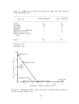 leakage to receiving bodies of water. In the Choptank drainage basin, crops
and respective planting methods are tabulated in Table 72 for the purpose of
projecting the herbicide leakage potentials (see Table 73). The approximated
7.5 percent no-till corn acreage planted (Parochetti, personal communication)
and 25.5 percent no-till soybeans (Maryland Department of Agriculture 1963-177,
1971-1977) have resulted in approximately 4,960 kg of paraquat applied to these
crops.
Alachlor, atrazine and linuron are the most widely used herbicides in the
Choptank area. A review of literature indicates that leakage figures for these
herbicides could potentially be 13 kg alachlor, 538 kg atrazine and 105 kg
linuron per year. If these loadings were diluted by the Choptank MLW volume
and not incorporated into the sediments, we would expect to find 0.36 ppb
atrazine, 0.07 ppb linuron and 0.0009 ppb alachlor. Less than a part per
trillion of trifluralin would be expected. This is assuming no net transport
out of (or into) the Choptank estuary. Although this latter assumption may be
somewhat simplistic, it may actually represent an underestimation of herbicide
loadings. In the Chester River there were researchers who found that more
pollutants were carried upstream from the mouth on sediments coming from the
Susquehanna River than were coming downstream.
Recent surveys of the Choptank River by the Chesapeake Bay Center for
Environmental Studies (CBCES) have provided some initial data on herbicide
levels and SAV populations at eight stations along the river from the mouth up
to Denton (Correll et al. 1977). Atrazine, linuron, trifluralin and alachlor
were analyzed from bottom sediments and filtered surface water. Alachlor was
found in low concentrations at only a few stations compared to higher and more
frequent concentrations of the other three herbicides.
Figures 42 and 43, Choptank River graph, show erratic levels of atrazine,
linuron and trifluralin in surface waters. Station 72, near the mouth of the
Choptank River, is the only station that was found to support submerged vegeta-
tion (Ruppia maritima Zannichellia palustris and Elodea canadensis despite
concentrations of linuron that had proved to be inhibitory to Zannichellia in
bioassays (see Table 74). Of special interest is the trend that is indicated
in Figure 44. Levels of linuron in bottom sediment sampled from the river mouth
upstream to Denton show a steady decrease in concentration. This is contrary
to what would be expected if excessive amounts of linuron were leaching into the
river from upstream soybean fields.
Another interesting aspect of Correll et al. data is that atrazine levels
in sufrace waters (dissolved) exceeded expectation levels based on the previous
calculations mentioned above. Field data indicated 2.0 ppb on the average and
the expected was 0.36 ppb. Also surprising is the fact that no atrazine was
reported in suspended sediments or the 0 to 3 cm sediment faction. However,
at station 77, atrazine was detected at a level of 3.83 ppm at a depth of 3 to
6 cm. The detection limit for atrazine in bottom sediment samples was 0.2 ppm.
Linuron, alachlor and trifluralin levels were found to be generally higher than
expected by calculations. This could indicate that there are continual concen-
tration build-ups or possibly other inputs into the mouth of the Choptank.
It is also possible that actual leakage rates are much higher than expected or
that CBCES has been identifying an artifact (Parochetti, personal communication)
instead of an herbicide.
216
image:
leakage to receiving bodies of water. In the Choptank drainage basin, crops
and respective planting methods are tabulated in Table 72 for the purpose of
projecting the herbicide leakage potentials (see Table 73). The approximated
7.5 percent no-till corn acreage planted (Parochetti, personal communication)
and 25.5 percent no-till soybeans (Maryland Department of Agriculture 1963-177,
1971-1977) have resulted in approximately 4,960 kg of paraquat applied to these
crops.
Alachlor, atrazine and linuron are the most widely used herbicides in the
Choptank area. A review of literature indicates that leakage figures for these
herbicides could potentially be 13 kg alachlor, 538 kg atrazine and 105 kg
linuron per year. If these loadings were diluted by the Choptank MLW volume
and not incorporated into the sediments, we would expect to find 0.36 ppb
atrazine, 0.07 ppb linuron and 0.0009 ppb alachlor. Less than a part per
trillion of trifluralin would be expected. This is assuming no net transport
out of (or into) the Choptank estuary. Although this latter assumption may be
somewhat simplistic, it may actually represent an underestimation of herbicide
loadings. In the Chester River there were researchers who found that more
pollutants were carried upstream from the mouth on sediments coming from the
Susquehanna River than were coming downstream.
Recent surveys of the Choptank River by the Chesapeake Bay Center for
Environmental Studies (CBCES) have provided some initial data on herbicide
levels and SAV populations at eight stations along the river from the mouth up
to Denton (Correll et al. 1977). Atrazine, linuron, trifluralin and alachlor
were analyzed from bottom sediments and filtered surface water. Alachlor was
found in low concentrations at only a few stations compared to higher and more
frequent concentrations of the other three herbicides.
Figures 42 and 43, Choptank River graph, show erratic levels of atrazine,
linuron and trifluralin in surface waters. Station 72, near the mouth of the
Choptank River, is the only station that was found to support submerged vegeta-
tion (Ruppia maritima Zannichellia palustris and Elodea canadensis despite
concentrations of linuron that had proved to be inhibitory to Zannichellia in
bioassays (see Table 74). Of special interest is the trend that is indicated
in Figure 44. Levels of linuron in bottom sediment sampled from the river mouth
upstream to Denton show a steady decrease in concentration. This is contrary
to what would be expected if excessive amounts of linuron were leaching into the
river from upstream soybean fields.
Another interesting aspect of Correll et al. data is that atrazine levels
in sufrace waters (dissolved) exceeded expectation levels based on the previous
calculations mentioned above. Field data indicated 2.0 ppb on the average and
the expected was 0.36 ppb. Also surprising is the fact that no atrazine was
reported in suspended sediments or the 0 to 3 cm sediment faction. However,
at station 77, atrazine was detected at a level of 3.83 ppm at a depth of 3 to
6 cm. The detection limit for atrazine in bottom sediment samples was 0.2 ppm.
Linuron, alachlor and trifluralin levels were found to be generally higher than
expected by calculations. This could indicate that there are continual concen-
tration build-ups or possibly other inputs into the mouth of the Choptank.
It is also possible that actual leakage rates are much higher than expected or
that CBCES has been identifying an artifact (Parochetti, personal communication)
instead of an herbicide.
216
image:
 Table 72. Estimates of total amount of specific
herbicides used for weed control in the Choptank
drainage basin, 1975a'b
Cropping
practice
No-till corn
Conventional
corn
Herbicide
Paraquat
Atrazine
Simazine
Paraquat
Alachlor
Atrazine
Atrazine
lAtrazine
[Alachlor
Atrazine
[Simazine
lAtrazine
[Simazine
[Atrazine
[Metolachlor
[Atrazine
[Butyl ate
No-till
soybeans
2,4-D
Paraquat
[Linuron
j_Alachlor
[Linuron
[Oryzalin
Concentional
corn
Linuron
Miscellaneous
Linuron
Alachlor
Linuron
Trifluralin
[Napthalamc
pinoseb
[Alachlor
Conventional
barley & wheat
2,4-D
Di camba
Rate
kg a.i./ha
0.27
1.37
1.37
0.27
2.20
1.65
2.20
1.10
1.65
1.10
1.10
1.10
1.65
1.10
1.65
1.10
3.30
0.42
0.55
1.10
1.65
0.55
0.55
0.83
1.10
1.65
1.65
0.83
0.83
1.10
1.65
1.65
0.42
0,14
Hectares
treated
2,194
157
7,249
13,048
3,479
870
1,559
1,450
1,450
7,654
6,506
383
612
153
14,535
2,236
2,684
1,118
3,687
1,843
Herbicide
kg a.i./ha
592
3,005
3,005
42
345
259
15,947
14,352
21,529
3,827
3,827
957
1,436
1,715
2,572
1,595
4,785
609
4,210
7,157
10.735
211
211
508
168
23,983
23,983
1,856
2,228
1,230
1,840
1,840
1,549
258
aParochetti, personal communication
^Maryland Department of .".grlc'jlt-re files 1977
cTrade name
217
image:
Table 72. Estimates of total amount of specific
herbicides used for weed control in the Choptank
drainage basin, 1975a'b
Cropping
practice
No-till corn
Conventional
corn
Herbicide
Paraquat
Atrazine
Simazine
Paraquat
Alachlor
Atrazine
Atrazine
lAtrazine
[Alachlor
Atrazine
[Simazine
lAtrazine
[Simazine
[Atrazine
[Metolachlor
[Atrazine
[Butyl ate
No-till
soybeans
2,4-D
Paraquat
[Linuron
j_Alachlor
[Linuron
[Oryzalin
Concentional
corn
Linuron
Miscellaneous
Linuron
Alachlor
Linuron
Trifluralin
[Napthalamc
pinoseb
[Alachlor
Conventional
barley & wheat
2,4-D
Di camba
Rate
kg a.i./ha
0.27
1.37
1.37
0.27
2.20
1.65
2.20
1.10
1.65
1.10
1.10
1.10
1.65
1.10
1.65
1.10
3.30
0.42
0.55
1.10
1.65
0.55
0.55
0.83
1.10
1.65
1.65
0.83
0.83
1.10
1.65
1.65
0.42
0,14
Hectares
treated
2,194
157
7,249
13,048
3,479
870
1,559
1,450
1,450
7,654
6,506
383
612
153
14,535
2,236
2,684
1,118
3,687
1,843
Herbicide
kg a.i./ha
592
3,005
3,005
42
345
259
15,947
14,352
21,529
3,827
3,827
957
1,436
1,715
2,572
1,595
4,785
609
4,210
7,157
10.735
211
211
508
168
23,983
23,983
1,856
2,228
1,230
1,840
1,840
1,549
258
aParochetti, personal communication
^Maryland Department of .".grlc'jlt-re files 1977
cTrade name
217
image:
 Table 73. Potential herbicide leakage, Choptank River drainage basin
Herbicide
Paraquat
Atrazine
Simazine
2,4-D
Dicamba
Trifluralin
Linuron
Alachlor
aData not available
bWu et al. 1977
cWhite et al. 1976
dWillis et al. 1975
Total
grams
applied
4,958,140
44,795,974
8,452,791
2,939,251
258,610
2,260,228
34,836,516
63,474,561
Possible
percent
leakage
a h
1.20b
a
0.21C
a
0.05d
0.30d
0.02b
Total
herbicide
leaked (grams)
a
537,551
a
6,172
a
1,130
104,509
12,694
fable 74. Summary of bioassay results of various concentrations
of atrazine and linuron on Zannichellia palustris9
Parameter
measured
Herbicide
concentration
Bioassay
results
Plant growth
Net 02 production
Gross photosynthesis
1 ppm atrazine
1 ppm linuron
1 ppm atrazine
10 ppm atrazine
100 ppm atrazine
1 ppm linuron
10 ppm linuron
100 ppm linuron
1 ppm atrazine
10 ppm atrazine
100 ppm atrazine
1 ppm linuron
10 ppm linuron
100 ppm linuron
increase
increase
increase until 20th
day then decrease
decrease
decrease
increase until 12th
day then decrease
decrease
increase
increase
decrease
decrease
decrease
decrease
decrease
aCorrell et al. 1977
Concentration for sediments.
adjusted to ppb level
Water column (dissolved) concentrations were
218
image:
Table 73. Potential herbicide leakage, Choptank River drainage basin
Herbicide
Paraquat
Atrazine
Simazine
2,4-D
Dicamba
Trifluralin
Linuron
Alachlor
aData not available
bWu et al. 1977
cWhite et al. 1976
dWillis et al. 1975
Total
grams
applied
4,958,140
44,795,974
8,452,791
2,939,251
258,610
2,260,228
34,836,516
63,474,561
Possible
percent
leakage
a h
1.20b
a
0.21C
a
0.05d
0.30d
0.02b
Total
herbicide
leaked (grams)
a
537,551
a
6,172
a
1,130
104,509
12,694
fable 74. Summary of bioassay results of various concentrations
of atrazine and linuron on Zannichellia palustris9
Parameter
measured
Herbicide
concentration
Bioassay
results
Plant growth
Net 02 production
Gross photosynthesis
1 ppm atrazine
1 ppm linuron
1 ppm atrazine
10 ppm atrazine
100 ppm atrazine
1 ppm linuron
10 ppm linuron
100 ppm linuron
1 ppm atrazine
10 ppm atrazine
100 ppm atrazine
1 ppm linuron
10 ppm linuron
100 ppm linuron
increase
increase
increase until 20th
day then decrease
decrease
decrease
increase until 12th
day then decrease
decrease
increase
increase
decrease
decrease
decrease
decrease
decrease
aCorrell et al. 1977
Concentration for sediments.
adjusted to ppb level
Water column (dissolved) concentrations were
218
image:
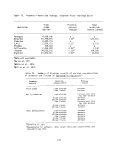 Further field work by Correll et al. has been performed on the Rhode and
Severn Rivers and the Poplar Islands. Figures 42 and 43 show herbicide concen-
trations of dissolved and suspended solids of surface water. Linuron shows
higher values at the river mouth (station 28) and atrazine and trifluralin are
higher in Muddy Creek (stations 30.2 and 31.5) for the filtered surface waters
in the Rhode River. This does not apply to suspended sediments concentrations
which tend to be rather random.
Figure 44 depicts concentration levels found in bottom sediment samples.
The two Muddy Creek stations exhibit the highest levels of all three herbicides.
No strong correlations can be made between these concentrations and SAV popula-
tions. Ruppia and Zannichellia were noted throughout the five Rhode River
stations despite what are considered to be inhibitory concentrations of linuron
at most of the stations. Station 29 produced the highest amount of biomass
(57,550 mg dry wt) yet showed almost 5 ppb linuron in suspended sediments and
over 2 ppm in bottom sediments. Stations 31.5 and 28 ranked next in biomass
(3,430 and 1,610 mg dry wt) despite higher herbicide concentrations than stations
28.4 and 30.2 which has lower plant biomass.
Similar work performed on the Severn River in June, 1976, shows the same
random concentrations over the length of the river (see Figure 42, 43 and 44).
Potamogeton pectinatus, P. perfoliatus, Myriophyllum spicatum and Ruppia maritima
were found in sparse quantities at stations 92 through 96 with the exception of
station 94 which supported about 30 times (11,410 mg dry wt) more vegetation than
station 95 (20 mg dry wt). In looking at the last two river stations together,
herbicide levels were higher than station 94, indicating possibly some correla-
tion between low biomass and high herbicide concentrations.
The fourth area surveyed was Poplar Island. Herbicide concentrations are
again random in relation to each of the three herbicides with the exception of
linuron and trifluralin levels which seem to follow more closely in the bottom
sediments than previously noted. Zannichellia, Ruppia and Potamogeton pectinatus
were found at station 81 (6,500 mg dry wt), station 82 (42,150 mg dry wt) and
station 83 (600 mg dry wt). High biomass at station 82 was composed primarily of
P. pectinatus. Herbicide concentrations at the same station indicate what bio-
assay analysis determined to be inhibitory levels of linuron and atrazine to
Zannichellia.
The lack of correlation between bioassay results and field data is confusing.
Clearly more herbicide studies are needed before a clearcut causality pattern
can be established. This is especially the case when many of the herbicide
values obtained by Correll et al. (1977) have not yet been confirmed by G-C mass-
spectrometer studies. Hopefully several studies now in the planning stages
(Stevenson, Kemp and Boynton; Stotts and Orth) may be able to resolve this con-
troversy.
Chesapeake Bay Area Herbicide Survey
In recent years, herbicide usage has increased in the Chesapeake Bay area.
In order to determine the extent of this increase, county agricultural exten-
sion agents from Maryland and Virginia were surveyed for information relating to
local use of nine common herbicides. Tables 75 and 76 tabulate the data from
the responding extension agents. These figures indicate a marked increase in
total herbicide use for all responding counties from 1971 to 1975.
219
image:
Further field work by Correll et al. has been performed on the Rhode and
Severn Rivers and the Poplar Islands. Figures 42 and 43 show herbicide concen-
trations of dissolved and suspended solids of surface water. Linuron shows
higher values at the river mouth (station 28) and atrazine and trifluralin are
higher in Muddy Creek (stations 30.2 and 31.5) for the filtered surface waters
in the Rhode River. This does not apply to suspended sediments concentrations
which tend to be rather random.
Figure 44 depicts concentration levels found in bottom sediment samples.
The two Muddy Creek stations exhibit the highest levels of all three herbicides.
No strong correlations can be made between these concentrations and SAV popula-
tions. Ruppia and Zannichellia were noted throughout the five Rhode River
stations despite what are considered to be inhibitory concentrations of linuron
at most of the stations. Station 29 produced the highest amount of biomass
(57,550 mg dry wt) yet showed almost 5 ppb linuron in suspended sediments and
over 2 ppm in bottom sediments. Stations 31.5 and 28 ranked next in biomass
(3,430 and 1,610 mg dry wt) despite higher herbicide concentrations than stations
28.4 and 30.2 which has lower plant biomass.
Similar work performed on the Severn River in June, 1976, shows the same
random concentrations over the length of the river (see Figure 42, 43 and 44).
Potamogeton pectinatus, P. perfoliatus, Myriophyllum spicatum and Ruppia maritima
were found in sparse quantities at stations 92 through 96 with the exception of
station 94 which supported about 30 times (11,410 mg dry wt) more vegetation than
station 95 (20 mg dry wt). In looking at the last two river stations together,
herbicide levels were higher than station 94, indicating possibly some correla-
tion between low biomass and high herbicide concentrations.
The fourth area surveyed was Poplar Island. Herbicide concentrations are
again random in relation to each of the three herbicides with the exception of
linuron and trifluralin levels which seem to follow more closely in the bottom
sediments than previously noted. Zannichellia, Ruppia and Potamogeton pectinatus
were found at station 81 (6,500 mg dry wt), station 82 (42,150 mg dry wt) and
station 83 (600 mg dry wt). High biomass at station 82 was composed primarily of
P. pectinatus. Herbicide concentrations at the same station indicate what bio-
assay analysis determined to be inhibitory levels of linuron and atrazine to
Zannichellia.
The lack of correlation between bioassay results and field data is confusing.
Clearly more herbicide studies are needed before a clearcut causality pattern
can be established. This is especially the case when many of the herbicide
values obtained by Correll et al. (1977) have not yet been confirmed by G-C mass-
spectrometer studies. Hopefully several studies now in the planning stages
(Stevenson, Kemp and Boynton; Stotts and Orth) may be able to resolve this con-
troversy.
Chesapeake Bay Area Herbicide Survey
In recent years, herbicide usage has increased in the Chesapeake Bay area.
In order to determine the extent of this increase, county agricultural exten-
sion agents from Maryland and Virginia were surveyed for information relating to
local use of nine common herbicides. Tables 75 and 76 tabulate the data from
the responding extension agents. These figures indicate a marked increase in
total herbicide use for all responding counties from 1971 to 1975.
219
image:
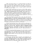 _a
CL
a.
4J
(O
10
9
8.
7
6
5
d)
o
71 72 73 74 75 76 77
Stations (upstream >)
Choptank River
78
10-
9
2" 8'
Q.
f"> — *
— 7
§6
'•£ 5'
(0
£4
E
S 3'
c
82-
1-
o
\J
r
*»••** * *
,««•* » ^ »
^ *
\ / x '
* j V
K x '/
91 92 93 94 95
Stations (upstream O
Severn River
4
*
1
'
jf
j?
>
^
96
10
9
§6
<o
i-
O)
Q.
Q.
c
o
10
9
r s
7
6
<a 5
|4
<u _
o 3
81 82 83
Stations
Poplar Island
84
l\
0
28 28.4 29 30.2
Stations (upstream - #
Rhode River
31.5
Linuron
• Atrazine
--"-'Trifluralin
• Biomass of Zannichellia palustris
(ppb X1000 = mg dry wt]
et al. 1977
Figure 42. Analysis of surface water (dissolved) and biomass, June, 1976a
220
image:
_a
CL
a.
4J
(O
10
9
8.
7
6
5
d)
o
71 72 73 74 75 76 77
Stations (upstream >)
Choptank River
78
10-
9
2" 8'
Q.
f"> — *
— 7
§6
'•£ 5'
(0
£4
E
S 3'
c
82-
1-
o
\J
r
*»••** * *
,««•* » ^ »
^ *
\ / x '
* j V
K x '/
91 92 93 94 95
Stations (upstream O
Severn River
4
*
1
'
jf
j?
>
^
96
10
9
§6
<o
i-
O)
Q.
Q.
c
o
10
9
r s
7
6
<a 5
|4
<u _
o 3
81 82 83
Stations
Poplar Island
84
l\
0
28 28.4 29 30.2
Stations (upstream - #
Rhode River
31.5
Linuron
• Atrazine
--"-'Trifluralin
• Biomass of Zannichellia palustris
(ppb X1000 = mg dry wt]
et al. 1977
Figure 42. Analysis of surface water (dissolved) and biomass, June, 1976a
220
image:
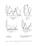 ^
o.
3
c
o
-I-)
c
O)
o
E
0
0
10'
9
8
7
6
5
4
3
2
1
0
,
\ *
• «
>x
*\ / * *
%* ** * *
V / '*••
^ \ X / \,/' '
\ X / / " v
10i
9
71 72 73 74 75
Stations (upstream -
Choptank River
T*
76
77
§6
•F~
^5
|4
•vV
91 92 93 94 95
Stations (upstream »)
Severn River
96
78
10
9
^•8
&7
10-
9
^7
c 6^
o
| 4
O> o
U -J
O o
O ^>
0^
81 82 83
Stations
Poplar Island
84
28 28.4 29 30.2
Stations (upstream
Rhode River
31.5
Linuron
Atrazine
Trifluralin
Biomass of Zannichellia palustris
(ppb X1000 = mg dry wt)
aCorrell et al. 1977
Figure 43. Analysis of surface water (suspended sediment) and biomass,
June, 1976a
221
image:
^
o.
3
c
o
-I-)
c
O)
o
E
0
0
10'
9
8
7
6
5
4
3
2
1
0
,
\ *
• «
>x
*\ / * *
%* ** * *
V / '*••
^ \ X / \,/' '
\ X / / " v
10i
9
71 72 73 74 75
Stations (upstream -
Choptank River
T*
76
77
§6
•F~
^5
|4
•vV
91 92 93 94 95
Stations (upstream »)
Severn River
96
78
10
9
^•8
&7
10-
9
^7
c 6^
o
| 4
O> o
U -J
O o
O ^>
0^
81 82 83
Stations
Poplar Island
84
28 28.4 29 30.2
Stations (upstream
Rhode River
31.5
Linuron
Atrazine
Trifluralin
Biomass of Zannichellia palustris
(ppb X1000 = mg dry wt)
aCorrell et al. 1977
Figure 43. Analysis of surface water (suspended sediment) and biomass,
June, 1976a
221
image:
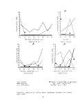 10<
9-
&7-
o
24-
c T
O) O '
o
1
0
10
9
8
to
OJ o
CJ 3
o
o
\
71
72 73 74 75
Stations (upstream -
Chootank Rivpr
76
4)
77
78
r
91 92 93 94 95
Statioins (upstream »)
Severn River
96
10
?
51
(O
c
cu
o
c
o
o
10
9-
8
T*
£
a.
c 6^
o
ai 3,
o °1
o ?•
ft*-
0-
if
81
82 83
Stations
Poplar Island
84
T
28 28.4 29 30.2
Stations (upstream )
Rhode River
31.5
Linulron
•Atrazine
Tritiluralin
Biomass of Zannichellia palustris
(ppm X1000 = mg dry wt)
aCorrell et al. 1977
Figure 44. Analysis of bottom sediment (0 to 3 cm) and biomass, June, 1976a
222
image:
10<
9-
&7-
o
24-
c T
O) O '
o
1
0
10
9
8
to
OJ o
CJ 3
o
o
\
71
72 73 74 75
Stations (upstream -
Chootank Rivpr
76
4)
77
78
r
91 92 93 94 95
Statioins (upstream »)
Severn River
96
10
?
51
(O
c
cu
o
c
o
o
10
9-
8
T*
£
a.
c 6^
o
ai 3,
o °1
o ?•
ft*-
0-
if
81
82 83
Stations
Poplar Island
84
T
28 28.4 29 30.2
Stations (upstream )
Rhode River
31.5
Linulron
•Atrazine
Tritiluralin
Biomass of Zannichellia palustris
(ppm X1000 = mg dry wt)
aCorrell et al. 1977
Figure 44. Analysis of bottom sediment (0 to 3 cm) and biomass, June, 1976a
222
image:
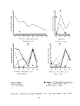 0
o
•1—
Q
u
3
S-
0)
V)
CU
0
s-
o
0
CU
c
'o
ro
CJ
o
ra
h~
p
C
CU
1 —
o
CU
o
in
en
•
,
en
•
LO
r-s
en
• —
en
•
LO
P-s.
en
"~
P-^.
en
• —
in
en
_
en
1
LO
I--
cn
r—
,—
cn
•
in
P-.
en
r-.
cn
co co o ^" en ^f i oin
Lo^tcoo-a-Locococo
LOLOCNli — r-*i — LO LO
r- CM
r-'vCOcnr-.cMcncnLOLO
CM CM IO ^ CO CO *± i — CM
CM <=r i — in i — co o
1— 1— r~"
.- CO <d- ^ CM CM LO *fr
o«^fOr— coooroi —
Px CTl CO CO *d" ^d~ ^" LO CO
•in** n r> r> *
r— • *d~ LO r— ro co ^j" ro
CM CM
^- CM CO LO rj- CM i — O CM
^rCcMLoi??Oa!§
rJ1 ,-T CM "d-* LO" CM* rfr" CO
co
rO^-«=l-COrO.— CMO^J-
0*1 I*-"* CD co P-*. c\i LO r**« CD
O *3~ CJ1 LO CM i — CVJP-xCT)
ro CM ro* i-^ co" i—" r-T r-T
• —
^" P""«. OO ^3 ^3 ^— t~~ C^O *^
CO ^" \Q LO LO ^3 CD ^3 ^3
i — rocvj^OLO ro p^. i — CNJ
r— CO OJ . — CO f— LO O
r-H I —
CMVOCOr-^
CO C\J i — COLT)* CO^DfO
C3 f*0 t^ CO *3~ UD CJ^ OJ
^~ •cj' 00 C\J ^}" kO
*^" r— CO
CO r*1" ^" r— P"^ CO LO
ro cr> i — o cri *d~ co
O LO <X) C\J LO CO
oooo^^cncMen^
to to *st" m in co CM 01 CM
« f\ * « M A t\
CM LO i— i— CM *3- O
ocMOLOr-cMOCOin
I^rCcorS^SLOLOoS
r— tO <" r— 00
CO . —
LO CCi — i — OOCMCM
c\i •* LO r~^ oo oo co co c\i
r^. CM r~» r-~ to to *3" ^«
CM CO CM
^* ^~ co en i-~ r-~ r^ ^~ oo
LO I— CO CM r— r^
c
•4-> eu cu a i.
rocc rcjas-co
3-^-^OJ3 CU 3 Or—
CTNN 1 £tni — S--C
i-S-E Oc-r-Cro
ra 4-> -r- * -r- «r- S- «r- i —
en
LO
LD" t/>
LO r-
ra
0
I-
CM
CO
in
en
^f
en
00
0 S-
r-. jg
en
LO CO
in
in
^
CO
CM
CM +->
•* J;
3;
ro
O
O
CM
5
^>
LO
n
r—
1 — t/l
-- CU
ro
r-. o
t£)
o
f—
o
*3" CU
• T3
01 c
O -3
r— S-
cn cu
S c
•!f
LO
0
CO
» CU
r- S-
.^
4_)
r— ra
CM. CQ
CO
CO
r—
ra
J-l
o
\-
in
en
^
i—
cn
r—
LO
CJ^
i —
c5
'
LO
P^s
Cft
"~
r-"
pv
CTt
LO
p-^.
cn
i —
,
en
r"~
LO
P-
cn
^-
cn
*~~~
LO
1 —
CP»
CTt
o^^-cop-.foocr>coc\)
OLOCTiCOi — «^* f*. CJ CSI
•Xi^O'd-ourorvcxjcoo
i — P^LOi — C^ r— LO LO
r— r—
^«^-r*-r-^'a-cTi, — f— co
COOCO«d-^O«tf-i£>(— OJ
co^-crtLD«cj-csjarror—
LD OJ i — LO CM LO
•
OCMCOLOi — f— P-. LO CO
LD O «* CJ^ i — <-
CD LO 00 LO
i — rocncocoi — r-cDcn
cop^aicn^cocncftcri
i— P^ LO C\J r— LO UD
O OJ C\J
*~
co LO r-. r- co r- •—
^t .^ cj* c\j •!< co vo Is** r*-*
CM c\j oj <— P-. r^.
^
OCOCOO CMrJ-^OOJ
p^. {Q I^Q ,__ ^c P^ CO t— • CM
•— U3CMLO CMCOCOP-
^O CM CM
O ^ O O
CO ^i~ i~~ ro
vo"
i — 00 OO P-. «^- P-»
CO^--K LD-K -)c CSJO^
• — LO CO CM CM LO
CO
^-P^Oi — LOLOLOO^-
OOOCOOO^tCOCD«^J-O
i — CD V£> i — CM
r- *d-OCMCOCO-— OCM
LOCOi — OCMt-^i — CMCM
00 LO i— LO i—
C
4-> OJ CU H3 i-
fO C C n3 -Q !L. C O
CTNJN 1 Et/>i — S-.C
S-t-E O C T- C n3
a +-> -r- * -i- -I- i_ •(- i —
CL<tC.OCMOah- I«=C
o
CO
LO
p*.
0
LO
^.J.
oo
to
LO
ro
LO
CO
en
CM
*
^_
LO
LO
rC
•~
px^
OO
*3-
LO
0
CO
«
CO
^-
CO
p*-.
LO
o
«l
o
*
o
CM
CM
LO
en
CO
CM
r^
1C
•p
0
t—
r^
en
'
CU
CU
3
-H
C
1— 1
o
C (U
.E .—
0 J3
CU ra
-p 1—
r— ra
o >
a. ra
•r- O
c c
CT ro
•i- ro
> -o
ro *
223
image:
0
o
•1—
Q
u
3
S-
0)
V)
CU
0
s-
o
0
CU
c
'o
ro
CJ
o
ra
h~
p
C
CU
1 —
o
CU
o
in
en
•
,
en
•
LO
r-s
en
• —
en
•
LO
P-s.
en
"~
P-^.
en
• —
in
en
_
en
1
LO
I--
cn
r—
,—
cn
•
in
P-.
en
r-.
cn
co co o ^" en ^f i oin
Lo^tcoo-a-Locococo
LOLOCNli — r-*i — LO LO
r- CM
r-'vCOcnr-.cMcncnLOLO
CM CM IO ^ CO CO *± i — CM
CM <=r i — in i — co o
1— 1— r~"
.- CO <d- ^ CM CM LO *fr
o«^fOr— coooroi —
Px CTl CO CO *d" ^d~ ^" LO CO
•in** n r> r> *
r— • *d~ LO r— ro co ^j" ro
CM CM
^- CM CO LO rj- CM i — O CM
^rCcMLoi??Oa!§
rJ1 ,-T CM "d-* LO" CM* rfr" CO
co
rO^-«=l-COrO.— CMO^J-
0*1 I*-"* CD co P-*. c\i LO r**« CD
O *3~ CJ1 LO CM i — CVJP-xCT)
ro CM ro* i-^ co" i—" r-T r-T
• —
^" P""«. OO ^3 ^3 ^— t~~ C^O *^
CO ^" \Q LO LO ^3 CD ^3 ^3
i — rocvj^OLO ro p^. i — CNJ
r— CO OJ . — CO f— LO O
r-H I —
CMVOCOr-^
CO C\J i — COLT)* CO^DfO
C3 f*0 t^ CO *3~ UD CJ^ OJ
^~ •cj' 00 C\J ^}" kO
*^" r— CO
CO r*1" ^" r— P"^ CO LO
ro cr> i — o cri *d~ co
O LO <X) C\J LO CO
oooo^^cncMen^
to to *st" m in co CM 01 CM
« f\ * « M A t\
CM LO i— i— CM *3- O
ocMOLOr-cMOCOin
I^rCcorS^SLOLOoS
r— tO <" r— 00
CO . —
LO CCi — i — OOCMCM
c\i •* LO r~^ oo oo co co c\i
r^. CM r~» r-~ to to *3" ^«
CM CO CM
^* ^~ co en i-~ r-~ r^ ^~ oo
LO I— CO CM r— r^
c
•4-> eu cu a i.
rocc rcjas-co
3-^-^OJ3 CU 3 Or—
CTNN 1 £tni — S--C
i-S-E Oc-r-Cro
ra 4-> -r- * -r- «r- S- «r- i —
en
LO
LD" t/>
LO r-
ra
0
I-
CM
CO
in
en
^f
en
00
0 S-
r-. jg
en
LO CO
in
in
^
CO
CM
CM +->
•* J;
3;
ro
O
O
CM
5
^>
LO
n
r—
1 — t/l
-- CU
ro
r-. o
t£)
o
f—
o
*3" CU
• T3
01 c
O -3
r— S-
cn cu
S c
•!f
LO
0
CO
» CU
r- S-
.^
4_)
r— ra
CM. CQ
CO
CO
r—
ra
J-l
o
\-
in
en
^
i—
cn
r—
LO
CJ^
i —
c5
'
LO
P^s
Cft
"~
r-"
pv
CTt
LO
p-^.
cn
i —
,
en
r"~
LO
P-
cn
^-
cn
*~~~
LO
1 —
CP»
CTt
o^^-cop-.foocr>coc\)
OLOCTiCOi — «^* f*. CJ CSI
•Xi^O'd-ourorvcxjcoo
i — P^LOi — C^ r— LO LO
r— r—
^«^-r*-r-^'a-cTi, — f— co
COOCO«d-^O«tf-i£>(— OJ
co^-crtLD«cj-csjarror—
LD OJ i — LO CM LO
•
OCMCOLOi — f— P-. LO CO
LD O «* CJ^ i — <-
CD LO 00 LO
i — rocncocoi — r-cDcn
cop^aicn^cocncftcri
i— P^ LO C\J r— LO UD
O OJ C\J
*~
co LO r-. r- co r- •—
^t .^ cj* c\j •!< co vo Is** r*-*
CM c\j oj <— P-. r^.
^
OCOCOO CMrJ-^OOJ
p^. {Q I^Q ,__ ^c P^ CO t— • CM
•— U3CMLO CMCOCOP-
^O CM CM
O ^ O O
CO ^i~ i~~ ro
vo"
i — 00 OO P-. «^- P-»
CO^--K LD-K -)c CSJO^
• — LO CO CM CM LO
CO
^-P^Oi — LOLOLOO^-
OOOCOOO^tCOCD«^J-O
i — CD V£> i — CM
r- *d-OCMCOCO-— OCM
LOCOi — OCMt-^i — CMCM
00 LO i— LO i—
C
4-> OJ CU H3 i-
fO C C n3 -Q !L. C O
CTNJN 1 Et/>i — S-.C
S-t-E O C T- C n3
a +-> -r- * -i- -I- i_ •(- i —
CL<tC.OCMOah- I«=C
o
CO
LO
p*.
0
LO
^.J.
oo
to
LO
ro
LO
CO
en
CM
*
^_
LO
LO
rC
•~
px^
OO
*3-
LO
0
CO
«
CO
^-
CO
p*-.
LO
o
«l
o
*
o
CM
CM
LO
en
CO
CM
r^
1C
•p
0
t—
r^
en
'
CU
CU
3
-H
C
1— 1
o
C (U
.E .—
0 J3
CU ra
-p 1—
r— ra
o >
a. ra
•r- O
c c
CT ro
•i- ro
> -o
ro *
223
image:
 r^
CT|
i— (
fO
c
•p"
O)
.,_
>
c
..'
c:
o
^^
>^
-Q
-~>
•
"r~
(0
" —
t/)
CD
-o
*|—
.,_
Q
O)
_c
T3
OJ
**
OJ
<L)
l/)
lf-
O
(1)
t/)
^
-l_)
q-
o
-p
<o
• p—
•M
LU
• ra
^o ^
p**. ^"^
a; i-i
-0 T5
^3 C
h- (0
^
c
£=
.c
U
S
i.
a>
ra
o
c
ra
ra
^
0)
_O
o
•o
c
ra
i
1/1
3
(U
CT
o
5
cn
2
£
ra
'^
i —
5
Q-
C
o
a.
<O
s-
o
a
c
u
a
LO
t-1
cn
LO
P-.
cn
r_
cn
LO
cn
cn
LO
2
r-.
LO
P-.
cn
i —
^
to
P-.
2
j^;
(—
LO
cn
i —
(
LO
P--.
en
•—
cn
*********
tO CM P-^ ^- •—,-•—
CM LO ^3- CM P-.
CM i—
r- cn o o to co .—
r— oo * r^ * p^co^-cn
«* CO CM •—
ro •—
LOVOOOr- r-P>,LO^
P^. CM CO CM i— LO CM
P*- CM CO r— CM
O tO f— CM i— OO LO *d"
^ ro ^ r— * co to r** i —
oo LO o t~~ r— cn cO
^- i — i —
OtOOLOOO-^OOCOCO
OO«tf-OCMtOCOO-)tDLO
r- CO i— •— CM ^J-
r— cn en e\j co r^ ^~ cn co
«d- CM CM co to co
*fr CM
encn^ooSSoocncn
co r-. co oo i— LO P-.
CO T— r-
i— CO ^" ^" tO ^— OO
O CO OJ CO •—
OJ i—
r— r— en oo cn
cnoo* LOto* * * LO
LO ^ t—
oo
OOOtOCXJI — OLOi — CO
LO r— i — 1 LO CO LO CO r™ ^~
cnooor-.^ r^^cn
<d-tOCOCMCM* LO.— CO
^-i^tO^"CM i — OCM
«3- CM r— >— CO
£
'r—
+j QJ aj ra S-
racc ra-ns-co
3 -r- >r- J3 <1J ^ O f—
CTN NO E Wi— S-^I
fO +> -r- * T- ••- ^ -i- i—
CL.«iCOeMOQH-_l<:
w
o
O)
* ra
0)
o.
ra
CM a;
CO 0
LO
o
4-
M-
LO 3
r- CO
«*
LO
cn
CM 4->
"~^ 01
CO T-
o
CM
O t—
" (/)
CTi i— •
CM
LO
CD v/
CM S-
O
r— >-
CO
LO
CO
10
LO
O -M
* C
cn <u
CM 2
o z
LO
a>
(U
=0
CO CT
LO cz
CO •!-
**
CM
*d- S-
tO 0)
tO LO
QJ
O
0
5
en
0 X
•* <u
« to
CO (U
•"" ^
•o
ra
o
to
1 —
r^
cn
'
LO
cn
r-
cn
LO
P-.
2
cn
LO
cn
cn
LO
2
cn
LO
P-.
en
i —
cn
LO
|^
cn
LO
cn
r--
l
LO
r-.
cn
f—
cn
r-. — coco^-tocnoo^-
i — LO LO i — COOi — tO LO~
LOOCMi — p-vOCOCM
5^rooScM§tn^
•— •— LOP^OOP*-Cnr— O
r— to »~~ o ^ en
«* r- r-
P-. CO LO i — CM CM
toio* cn* CM* cnLo
co en ^~ o r%. cn
oo og i— •— <n
^J-COLOO cM^-r^cn
CM co CM o to r^
LO •— «=r oo
CM 1 — CTl tO CM OO LO
OP-.OOO* CO »— * CO
i— cn •— oo oo i— LO
O CM CM «3-
i— r— CM
LO ^~ cn r*^. ^3- co
O LO CO CM CO CM
* r- o + * r-.
o •—
""
co cn
tO CM * LO CO OO
O <d- CM * -K CM *
•— i—
enocMScoSoooocn
^- t^- LO r— tO i — tO »~
CO r— CM
^- to F— r- cocncoto
r*-^ CM co to to CD^
^- oo
•K<y* LOCM** * LO
r,
CO
^fCMCOLOLOi — COCOtO
CM CO CM r— CO CNJ CM
P^ CM CM CM CD
tO P"-" tO ^" CO O OO OO
I~K ' ' *
"° •"
o^cor-^-^-^^-^
oo .— o LO cMrocor^
LO CM r —
QQ Si " ^±
O CM CO CO
CM ^~
c
^
+J <D Q} ra s-
race ra-Qi-co
U .,_.,_ JD 0) 3 0 •—
CTN NO E t/li — S-.C
ra ra ra i ro o *^~ 3 <j
ra +-> -1- " T- ~r~ ^ T- r—
O-<CCOCMOO(— — 1«=C
CO
LO
LO
cn
CO
^j.
co
LO
S
1 —
*
*
,_r
LO
CO
LO
o
^_
LO
r*-
CO
to
CM
r~~
^
CD
cn
cn
CM
cn
en
o
„
0
•
CO
LO
^"
1*^.
cn
LO
CM
CD
„
CO
to
o
cn
i—
•~~
CM
CD
LO
ra
o
1—
^
r»».
cn
0)
i*-
OJ
-t-)
4->
to
C
>— 1
u
'£
0
QJ
>,
'o
D_
ra
c:
cn
s_
>
ra
224
image:
r^
CT|
i— (
fO
c
•p"
O)
.,_
>
c
..'
c:
o
^^
>^
-Q
-~>
•
"r~
(0
" —
t/)
CD
-o
*|—
.,_
Q
O)
_c
T3
OJ
**
OJ
<L)
l/)
lf-
O
(1)
t/)
^
-l_)
q-
o
-p
<o
• p—
•M
LU
• ra
^o ^
p**. ^"^
a; i-i
-0 T5
^3 C
h- (0
^
c
£=
.c
U
S
i.
a>
ra
o
c
ra
ra
^
0)
_O
o
•o
c
ra
i
1/1
3
(U
CT
o
5
cn
2
£
ra
'^
i —
5
Q-
C
o
a.
<O
s-
o
a
c
u
a
LO
t-1
cn
LO
P-.
cn
r_
cn
LO
cn
cn
LO
2
r-.
LO
P-.
cn
i —
^
to
P-.
2
j^;
(—
LO
cn
i —
(
LO
P--.
en
•—
cn
*********
tO CM P-^ ^- •—,-•—
CM LO ^3- CM P-.
CM i—
r- cn o o to co .—
r— oo * r^ * p^co^-cn
«* CO CM •—
ro •—
LOVOOOr- r-P>,LO^
P^. CM CO CM i— LO CM
P*- CM CO r— CM
O tO f— CM i— OO LO *d"
^ ro ^ r— * co to r** i —
oo LO o t~~ r— cn cO
^- i — i —
OtOOLOOO-^OOCOCO
OO«tf-OCMtOCOO-)tDLO
r- CO i— •— CM ^J-
r— cn en e\j co r^ ^~ cn co
«d- CM CM co to co
*fr CM
encn^ooSSoocncn
co r-. co oo i— LO P-.
CO T— r-
i— CO ^" ^" tO ^— OO
O CO OJ CO •—
OJ i—
r— r— en oo cn
cnoo* LOto* * * LO
LO ^ t—
oo
OOOtOCXJI — OLOi — CO
LO r— i — 1 LO CO LO CO r™ ^~
cnooor-.^ r^^cn
<d-tOCOCMCM* LO.— CO
^-i^tO^"CM i — OCM
«3- CM r— >— CO
£
'r—
+j QJ aj ra S-
racc ra-ns-co
3 -r- >r- J3 <1J ^ O f—
CTN NO E Wi— S-^I
fO +> -r- * T- ••- ^ -i- i—
CL.«iCOeMOQH-_l<:
w
o
O)
* ra
0)
o.
ra
CM a;
CO 0
LO
o
4-
M-
LO 3
r- CO
«*
LO
cn
CM 4->
"~^ 01
CO T-
o
CM
O t—
" (/)
CTi i— •
CM
LO
CD v/
CM S-
O
r— >-
CO
LO
CO
10
LO
O -M
* C
cn <u
CM 2
o z
LO
a>
(U
=0
CO CT
LO cz
CO •!-
**
CM
*d- S-
tO 0)
tO LO
QJ
O
0
5
en
0 X
•* <u
« to
CO (U
•"" ^
•o
ra
o
to
1 —
r^
cn
'
LO
cn
r-
cn
LO
P-.
2
cn
LO
cn
cn
LO
2
cn
LO
P-.
en
i —
cn
LO
|^
cn
LO
cn
r--
l
LO
r-.
cn
f—
cn
r-. — coco^-tocnoo^-
i — LO LO i — COOi — tO LO~
LOOCMi — p-vOCOCM
5^rooScM§tn^
•— •— LOP^OOP*-Cnr— O
r— to »~~ o ^ en
«* r- r-
P-. CO LO i — CM CM
toio* cn* CM* cnLo
co en ^~ o r%. cn
oo og i— •— <n
^J-COLOO cM^-r^cn
CM co CM o to r^
LO •— «=r oo
CM 1 — CTl tO CM OO LO
OP-.OOO* CO »— * CO
i— cn •— oo oo i— LO
O CM CM «3-
i— r— CM
LO ^~ cn r*^. ^3- co
O LO CO CM CO CM
* r- o + * r-.
o •—
""
co cn
tO CM * LO CO OO
O <d- CM * -K CM *
•— i—
enocMScoSoooocn
^- t^- LO r— tO i — tO »~
CO r— CM
^- to F— r- cocncoto
r*-^ CM co to to CD^
^- oo
•K<y* LOCM** * LO
r,
CO
^fCMCOLOLOi — COCOtO
CM CO CM r— CO CNJ CM
P^ CM CM CM CD
tO P"-" tO ^" CO O OO OO
I~K ' ' *
"° •"
o^cor-^-^-^^-^
oo .— o LO cMrocor^
LO CM r —
QQ Si " ^±
O CM CO CO
CM ^~
c
^
+J <D Q} ra s-
race ra-Qi-co
U .,_.,_ JD 0) 3 0 •—
CTN NO E t/li — S-.C
ra ra ra i ro o *^~ 3 <j
ra +-> -1- " T- ~r~ ^ T- r—
O-<CCOCMOO(— — 1«=C
CO
LO
LO
cn
CO
^j.
co
LO
S
1 —
*
*
,_r
LO
CO
LO
o
^_
LO
r*-
CO
to
CM
r~~
^
CD
cn
cn
CM
cn
en
o
„
0
•
CO
LO
^"
1*^.
cn
LO
CM
CD
„
CO
to
o
cn
i—
•~~
CM
CD
LO
ra
o
1—
^
r»».
cn
0)
i*-
OJ
-t-)
4->
to
C
>— 1
u
'£
0
QJ
>,
'o
D_
ra
c:
cn
s_
>
ra
224
image:
 CHLORINE
Since the early 19th century, chlorine has been utilized as a sanitizing
agent. By 1912, it was widely used for the destruction of bacteria in both
sewage and potable waters (Schultze 1974). Chlorine has been found to be
effective for:
disinfection of clams and oysters prior to marketing
. control of midge larvae and alage in swimming pools
controlling taste and ordor in municipal water supplies
. sterilization of fish hatchery water supplies
reduction in biochemical oxygen demand of domestic wastewater
odor and fly control in wastewater treatment plants
. industrial wastes
. antifoul ing in heat exchangers and piping of water cooling systems
. pulp and paper production (bleach)
. herbicide and pesticide production
The ecological impact of this strong oxidant and its by-products on the
marine environment appears to be vast. It was vertified several years ago
that chlorinated hydrocarbons such as DDT and DDE, dieldrin and PCBs which
enter seawaters from land runoff, sewage outfalls and the atmosphere were
extremely dangerous to marine flora and fauna .(Goldberg et al. 1971).
Goldberg et al. (1971) cited the work of Nimmo et al. (1970) who found
that continuous exposure of 0.2 ppb chlorinated hydrocarbon killed shrimp.
They also refer to Duke et al. (1970) who determined that one ppb of the PCB
Arcolor 1254 caused a 20 percent decrease in oyster shell growth. Duke corre-
lated HC1 residues in mollusks to nearby agricultural chemical applications.
Fish and birds have also exhibited negative effects due to chlorinated
compounds. Concentrations of chlorine in lipid ovary tissues affected new
born growth. A 5 ppm chlorine residual caused developmental failure of sac
drys containing young fish (Goldberg et al. 1972). Deaths of bald eagles
(Mulhern et al. 1970), common loon (Butler 1966) and peregrine falcons (Jeffries
and Prestt 1966) are caused by chlorinated hydrocarbons through eggshell
thinning (Goldsberg et al. 1971). Bald eagles and peregrine falcons are in-
cluded on the Department of the Interior's endangered species list.
Aquatic research has demonstrated that phytoplankton show decreased
growth, developmental failures and increased mortality rates in response to
225
image:
CHLORINE
Since the early 19th century, chlorine has been utilized as a sanitizing
agent. By 1912, it was widely used for the destruction of bacteria in both
sewage and potable waters (Schultze 1974). Chlorine has been found to be
effective for:
disinfection of clams and oysters prior to marketing
. control of midge larvae and alage in swimming pools
controlling taste and ordor in municipal water supplies
. sterilization of fish hatchery water supplies
reduction in biochemical oxygen demand of domestic wastewater
odor and fly control in wastewater treatment plants
. industrial wastes
. antifoul ing in heat exchangers and piping of water cooling systems
. pulp and paper production (bleach)
. herbicide and pesticide production
The ecological impact of this strong oxidant and its by-products on the
marine environment appears to be vast. It was vertified several years ago
that chlorinated hydrocarbons such as DDT and DDE, dieldrin and PCBs which
enter seawaters from land runoff, sewage outfalls and the atmosphere were
extremely dangerous to marine flora and fauna .(Goldberg et al. 1971).
Goldberg et al. (1971) cited the work of Nimmo et al. (1970) who found
that continuous exposure of 0.2 ppb chlorinated hydrocarbon killed shrimp.
They also refer to Duke et al. (1970) who determined that one ppb of the PCB
Arcolor 1254 caused a 20 percent decrease in oyster shell growth. Duke corre-
lated HC1 residues in mollusks to nearby agricultural chemical applications.
Fish and birds have also exhibited negative effects due to chlorinated
compounds. Concentrations of chlorine in lipid ovary tissues affected new
born growth. A 5 ppm chlorine residual caused developmental failure of sac
drys containing young fish (Goldberg et al. 1972). Deaths of bald eagles
(Mulhern et al. 1970), common loon (Butler 1966) and peregrine falcons (Jeffries
and Prestt 1966) are caused by chlorinated hydrocarbons through eggshell
thinning (Goldsberg et al. 1971). Bald eagles and peregrine falcons are in-
cluded on the Department of the Interior's endangered species list.
Aquatic research has demonstrated that phytoplankton show decreased
growth, developmental failures and increased mortality rates in response to
225
image:
 chlorine. Chlorine inhibits photosynthesis in single-celled marine plants
causing these effects. Particularly important is that these plants may be
a vehicle for transferring these potentially toxic compounds to higher trophic
levels (Goldberg et al. 1971).
In bioassay tanks using estuarine waters, Wester and Rawles (1976)
described symptoms in aquatic macrophytes of growth retardation, loss of
chlorophyll and collapse when total available chlorine levels ranged from
0.05 to 0.125 ppm. "Field observations, plot studies and data from controlled
environment investigations with Ca boma ca ro1i n i a n a, El odea canadensis,
Potamogeton crispus, £. pectinatus and Vallisneria spiral is indicate that
chlorine pollution may be a significant cause of this critical environmental
problem affecting these once locally prevalent plants"
The fate of chlorine in estuarine ecosystems is largely unknown at the
present time and laboratory chemistry techniques for chlorine are not depend-
able yet (Davis, personal communication). Experimental data does show that
chlorine acts differently in marine waters compared to freshwaters. The 60 ppm
of bromide that characterizes marine waters is readily oxidized by the intro-
duction of strong oxidants. In marine waters, the resulting compounds are
brominated while in freshwater, analagous chlorinated compounds are formed
(Sugam and Helz 1977; Davis et al. 1977). An estimate of the possible number of
theoretical halogenated inorganic and organic by-products produced is 1,500
(Davis, personal communication). The measurement of these compounds requires
an intensive inventory and analytical effort. The common technique for measur-
ing the active oxidative stage or residual chlorine is the amperometric
titrator method. This technique does not accurately record hypobromite and
bromate or give any clue to the number of halogenated by-products (Davis et al.
1977).
In the Chesapeake Bay, chlorine and chlorine by-products enter the estuary
via sewage treatment plants, water treatment and cooling waters from electric
power plants, run-off from agricultural pesticide application and industrial
effluents. The amount of chlorine used for sewage treatment has been estimated
as ten times the amount used as biocide for power production cooling waters
(Block et al. 1977). Based on 1973 data available from Martin Marietta Corpora-
tion (Polgar, personal communication), it has been estimated that chlorine used
in municipal treatment is 12,200,000 kg and 7,000,000 kg is applied by
power generating facilities. Jolley, in a 1975 symposium on the environmental
impacts of water chlorination, estimated that at least 3 percent of this input
could produce halogenated organic species of a persistent nature (Davis and
Middaugh 1975).
A survey of chlorine usage from sewage treatment plants in the Chesapeake
Bay shows an increase greater than 2.5 times from 1971 to 1975 (see Table 77)
in each of four river systems that were analyzed.
There is currently no direct measurable evidence relating the Baywide
decline in submerged aquatic vegetation to levels of chlorination. Bay
vegetation was at its lowest point in 1975 but has increased in subsequent
years. This does not clearly correlate with chlorine inputs which have
226
image:
chlorine. Chlorine inhibits photosynthesis in single-celled marine plants
causing these effects. Particularly important is that these plants may be
a vehicle for transferring these potentially toxic compounds to higher trophic
levels (Goldberg et al. 1971).
In bioassay tanks using estuarine waters, Wester and Rawles (1976)
described symptoms in aquatic macrophytes of growth retardation, loss of
chlorophyll and collapse when total available chlorine levels ranged from
0.05 to 0.125 ppm. "Field observations, plot studies and data from controlled
environment investigations with Ca boma ca ro1i n i a n a, El odea canadensis,
Potamogeton crispus, £. pectinatus and Vallisneria spiral is indicate that
chlorine pollution may be a significant cause of this critical environmental
problem affecting these once locally prevalent plants"
The fate of chlorine in estuarine ecosystems is largely unknown at the
present time and laboratory chemistry techniques for chlorine are not depend-
able yet (Davis, personal communication). Experimental data does show that
chlorine acts differently in marine waters compared to freshwaters. The 60 ppm
of bromide that characterizes marine waters is readily oxidized by the intro-
duction of strong oxidants. In marine waters, the resulting compounds are
brominated while in freshwater, analagous chlorinated compounds are formed
(Sugam and Helz 1977; Davis et al. 1977). An estimate of the possible number of
theoretical halogenated inorganic and organic by-products produced is 1,500
(Davis, personal communication). The measurement of these compounds requires
an intensive inventory and analytical effort. The common technique for measur-
ing the active oxidative stage or residual chlorine is the amperometric
titrator method. This technique does not accurately record hypobromite and
bromate or give any clue to the number of halogenated by-products (Davis et al.
1977).
In the Chesapeake Bay, chlorine and chlorine by-products enter the estuary
via sewage treatment plants, water treatment and cooling waters from electric
power plants, run-off from agricultural pesticide application and industrial
effluents. The amount of chlorine used for sewage treatment has been estimated
as ten times the amount used as biocide for power production cooling waters
(Block et al. 1977). Based on 1973 data available from Martin Marietta Corpora-
tion (Polgar, personal communication), it has been estimated that chlorine used
in municipal treatment is 12,200,000 kg and 7,000,000 kg is applied by
power generating facilities. Jolley, in a 1975 symposium on the environmental
impacts of water chlorination, estimated that at least 3 percent of this input
could produce halogenated organic species of a persistent nature (Davis and
Middaugh 1975).
A survey of chlorine usage from sewage treatment plants in the Chesapeake
Bay shows an increase greater than 2.5 times from 1971 to 1975 (see Table 77)
in each of four river systems that were analyzed.
There is currently no direct measurable evidence relating the Baywide
decline in submerged aquatic vegetation to levels of chlorination. Bay
vegetation was at its lowest point in 1975 but has increased in subsequent
years. This does not clearly correlate with chlorine inputs which have
226
image:
 increased substantially every year in the 1970s due to increased use by sewage
treatment plants and power plants. Lower rainfall in 1976 and 1977 provided
less potential fresh water dilution of the increasing chlorine load. Therefore,
if chlorine alone is suspect as the agent causing Baywide declines of aquatic
vegetation, we would expect to see a continued decline in SAV after 1975. This
has not been found to be the case. Therefore, either chlorine is not at fault
or it is acting synergistically with other factors.
However, in areas of the Bay which have high concentrations of both power
plants, which use chlorine in large pulses to reduce fouling organisms, and
STPs, there is a likelihood that chlorine may be a significant factor. The
Department of the Interior, National Ecological Services Lab has a continuing
monitoring and chlorine bioassay program which should provide a definitive
answer concerning the extent of chlorine impacts on SAV in the future (Wester,
personal communication). Therefore, although chlorine may be an important
factor in causing SAV declines in population impacted watersheds of the Western
Shore, there is little evidence presently linking it as a prime factor to the
Baywide submerged aquatic decline. Any impact to SAV from chlorine can only
be speculative at this point. However, this conclusion must be considered as
tentative until a better working knowledge of the complete chemistry of chlorine
is available for the Chesapeake Bay.
Table 77. Chlorine usage in four major rivers of the Chesapeake Bay
estuary, 1971 and 1975a
River 1971 1975
Patuxent River
Pocomoke River
Chester River
Choptank River
TOTAL
5,100
350
140
1,500
70,090
15,125
700
550
3,600
19,975
Maryland Department of Health and Mental Hygiene, Environmental
Health Administration files 1977.
TURBIDITY
Turbidity refers to a variety of water quality parameters which include
suspended organic and inorganic particulates, coloring or staining from dis-
solved organic matter and plankton. These varying components of turbidity
227
image:
increased substantially every year in the 1970s due to increased use by sewage
treatment plants and power plants. Lower rainfall in 1976 and 1977 provided
less potential fresh water dilution of the increasing chlorine load. Therefore,
if chlorine alone is suspect as the agent causing Baywide declines of aquatic
vegetation, we would expect to see a continued decline in SAV after 1975. This
has not been found to be the case. Therefore, either chlorine is not at fault
or it is acting synergistically with other factors.
However, in areas of the Bay which have high concentrations of both power
plants, which use chlorine in large pulses to reduce fouling organisms, and
STPs, there is a likelihood that chlorine may be a significant factor. The
Department of the Interior, National Ecological Services Lab has a continuing
monitoring and chlorine bioassay program which should provide a definitive
answer concerning the extent of chlorine impacts on SAV in the future (Wester,
personal communication). Therefore, although chlorine may be an important
factor in causing SAV declines in population impacted watersheds of the Western
Shore, there is little evidence presently linking it as a prime factor to the
Baywide submerged aquatic decline. Any impact to SAV from chlorine can only
be speculative at this point. However, this conclusion must be considered as
tentative until a better working knowledge of the complete chemistry of chlorine
is available for the Chesapeake Bay.
Table 77. Chlorine usage in four major rivers of the Chesapeake Bay
estuary, 1971 and 1975a
River 1971 1975
Patuxent River
Pocomoke River
Chester River
Choptank River
TOTAL
5,100
350
140
1,500
70,090
15,125
700
550
3,600
19,975
Maryland Department of Health and Mental Hygiene, Environmental
Health Administration files 1977.
TURBIDITY
Turbidity refers to a variety of water quality parameters which include
suspended organic and inorganic particulates, coloring or staining from dis-
solved organic matter and plankton. These varying components of turbidity
227
image:
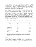 can affect submerged aquatics in different ways. Participates can physically
block the penetration of light through the water column. Stained or colored
waters diffently absorb various wavelengths of sunlight. Plankton can cause
scums, mats or blooms which physically block sunlight and directly utlize red
and blue wavelengths for photosynthesis. The dissolved and participate matter
entering the water column can serve as a vehicle for the introduction of
soluble pollutants into an estuary. Whether these pollutants are heavy metals,
greasy wastes, agro-chemicals, excessive nutrients, etc., they can be diluted,
absorbed into substrate material, oxidized or precipitated.
Turbidity not only varies as to components but has high seasonal vari-
ability. Winter usually is the period of lowest turbidity. The spring rains
increase suspended solids loading, and warming temperatures in summer promote
plankton blooms. In addition, storms throughout the year can resuspend bottom
sediments causing short periods of high turbidity.
Sources of suspended particulates are categorized by Biggs (1970) as:
external, from freshwater runoff; marginal, from shoreline erosion; and
internal, from biological production. In studying the Chesapeake Bay, Biggs
estimated a yearly suspended solids input based on the year February 1, 1966
to January 31, 1967. The net volume of introduced sediments for the upper Bay
(above Annapolis) was estimated as 1.6 x 10⁶m3 and 0.8 x 10bm3 for the central
Bay (from Annapolis to a point just south of the Patuxent River mouth). With
uniform distribution, the nominal rates of sedimentation would be 3.7 mm/year
.for the upper Bay and 1.1 mm/year for the central Bay.
The impact of suspended solids on SAV is not wholly negative. The depo-
sition of silt and clay particles can aid in building up suitable bottom sub-
strates in barren areas or add nutrients to existing substrates (Odum and
Wilson 1962). Submerged aquatic vegetation, in turn, aids in the settling out
of suspended solids.
Turbidity has often been implicated as a prime cause for the decline of
submerged vegetation in the Chesapeake Bay (Martin and Uhler 1939; Bayley
et al. in press; Rawls et al. 1975). However, the Bay has always been turbid
from natural causes, due to the dynamic nature of a wind driven estuary. Many
people knowledgeable about the Bay feel that turbidities have increased drama-
tically over the last forty years. Logically this would seem to be valid.
Increased boat traffic and shoreline construction alone would appear to have
augmented turbidity levels. However, the data available from the Department
of Natural Resouces show that yearly averages of suspended solids in the
Maryland portion of the Bay have declined in the 1970s (see Table 78). Further-
more, there is a positive correlation (r=.58) of SAV overall occurrences and
yearly average turbiditity levels. This is in the opposite direction expected,
assuming that high sediment loadings and resulting turbidities inhibit plant
growth. Focusing on the turbidities during the growing season (April to
September) (see Table 78), there is a little more reasonable trend.
The year of highest suspended solids during the growing season was 1975,
also the year of lowest submerged aquatic vegetation occurrence. However, this
does little to demonstrate that a clear relationship exists between growing
228
image:
can affect submerged aquatics in different ways. Participates can physically
block the penetration of light through the water column. Stained or colored
waters diffently absorb various wavelengths of sunlight. Plankton can cause
scums, mats or blooms which physically block sunlight and directly utlize red
and blue wavelengths for photosynthesis. The dissolved and participate matter
entering the water column can serve as a vehicle for the introduction of
soluble pollutants into an estuary. Whether these pollutants are heavy metals,
greasy wastes, agro-chemicals, excessive nutrients, etc., they can be diluted,
absorbed into substrate material, oxidized or precipitated.
Turbidity not only varies as to components but has high seasonal vari-
ability. Winter usually is the period of lowest turbidity. The spring rains
increase suspended solids loading, and warming temperatures in summer promote
plankton blooms. In addition, storms throughout the year can resuspend bottom
sediments causing short periods of high turbidity.
Sources of suspended particulates are categorized by Biggs (1970) as:
external, from freshwater runoff; marginal, from shoreline erosion; and
internal, from biological production. In studying the Chesapeake Bay, Biggs
estimated a yearly suspended solids input based on the year February 1, 1966
to January 31, 1967. The net volume of introduced sediments for the upper Bay
(above Annapolis) was estimated as 1.6 x 10⁶m3 and 0.8 x 10bm3 for the central
Bay (from Annapolis to a point just south of the Patuxent River mouth). With
uniform distribution, the nominal rates of sedimentation would be 3.7 mm/year
.for the upper Bay and 1.1 mm/year for the central Bay.
The impact of suspended solids on SAV is not wholly negative. The depo-
sition of silt and clay particles can aid in building up suitable bottom sub-
strates in barren areas or add nutrients to existing substrates (Odum and
Wilson 1962). Submerged aquatic vegetation, in turn, aids in the settling out
of suspended solids.
Turbidity has often been implicated as a prime cause for the decline of
submerged vegetation in the Chesapeake Bay (Martin and Uhler 1939; Bayley
et al. in press; Rawls et al. 1975). However, the Bay has always been turbid
from natural causes, due to the dynamic nature of a wind driven estuary. Many
people knowledgeable about the Bay feel that turbidities have increased drama-
tically over the last forty years. Logically this would seem to be valid.
Increased boat traffic and shoreline construction alone would appear to have
augmented turbidity levels. However, the data available from the Department
of Natural Resouces show that yearly averages of suspended solids in the
Maryland portion of the Bay have declined in the 1970s (see Table 78). Further-
more, there is a positive correlation (r=.58) of SAV overall occurrences and
yearly average turbiditity levels. This is in the opposite direction expected,
assuming that high sediment loadings and resulting turbidities inhibit plant
growth. Focusing on the turbidities during the growing season (April to
September) (see Table 78), there is a little more reasonable trend.
The year of highest suspended solids during the growing season was 1975,
also the year of lowest submerged aquatic vegetation occurrence. However, this
does little to demonstrate that a clear relationship exists between growing
228
image:
 season suspended solids and SAV declines, This is because the average suspend-
ed solids for the growing seasons of 1967 to 1969 was 54.3 mg/1 compared to
23.8 mg/1 recorded in the 1970s. This decrease occurred during a period when
SAVs were declining. This second positive correlation adds to the doubt that
SAV disappearances can be attributed alone to increasing turbidity effects
due to increasing levels of suspended sediment.
Table 78. Yearly averages of suspended solids (mg/1), Maryland
Chesapeake Bay, 1971-1976a
Year
Suspended solids (mg/1)
Apr/May
June/Jly
Aug/Sept Apr/Sept Average
1971
1972
1973
1974
1975
1976
32.0
37.8
9.0
25.8
36.5
12.0
26.3
-
7.0
40.3
28.7
23.7
14.4
5.5
6.8
26.5
59.2
15.9
24.2
21.6
7.6
30.9
41.5
17.2
30.1
32.9
7.6
29.4
27.4
21.7
Maryland Department of Water Resources files 1977
Francis Uhler (Patuxent Wildlife Station, U.S. Fish and Wildlife Service)
and Vernon Stotts (Maryland Wildlife Administration) maintain that the absence
of submerged aquatics in an area such as Nanticoke River is due to higher tur-
bidities (personal communications). However, Maryland Department of Natural
Resources water quality data show that in the period 1966 to 1976 the
Nanticoke actually had lower suspended solids (33.9 mg/1) than the Choptank
(36.6 mg/1) or Chester (41.5 mg/1). Also, in most tributaries in the Bay,
the suspended solids were lower in the 1970s than in the 1960s. This again
suggests thai; it is difficult to attribute submerged aquatic declines in the
1970s to turbidity alone (see Figure 45).
Experimental evidence relating directly to the effects of Chesapeake Bay
turbidity on SAV is scarce, at least until recently. Field surveys conducted
by the Chesapeake Bay Center for Environmental Studies (Smithsonian Institu-
tion) in the Rhode and Severn Rivers do not indicate a strong correlation be-
tween turbidity and SAV occurrence. In both rivers, the greatest abundance of
SAV was found in the areas of maximum turbidity where the fresh and brackish
waters meet. However, in the Choptank River, vegetation was not found above
Cambridge where the zone of maximum turbidity is located.
229
image:
season suspended solids and SAV declines, This is because the average suspend-
ed solids for the growing seasons of 1967 to 1969 was 54.3 mg/1 compared to
23.8 mg/1 recorded in the 1970s. This decrease occurred during a period when
SAVs were declining. This second positive correlation adds to the doubt that
SAV disappearances can be attributed alone to increasing turbidity effects
due to increasing levels of suspended sediment.
Table 78. Yearly averages of suspended solids (mg/1), Maryland
Chesapeake Bay, 1971-1976a
Year
Suspended solids (mg/1)
Apr/May
June/Jly
Aug/Sept Apr/Sept Average
1971
1972
1973
1974
1975
1976
32.0
37.8
9.0
25.8
36.5
12.0
26.3
-
7.0
40.3
28.7
23.7
14.4
5.5
6.8
26.5
59.2
15.9
24.2
21.6
7.6
30.9
41.5
17.2
30.1
32.9
7.6
29.4
27.4
21.7
Maryland Department of Water Resources files 1977
Francis Uhler (Patuxent Wildlife Station, U.S. Fish and Wildlife Service)
and Vernon Stotts (Maryland Wildlife Administration) maintain that the absence
of submerged aquatics in an area such as Nanticoke River is due to higher tur-
bidities (personal communications). However, Maryland Department of Natural
Resources water quality data show that in the period 1966 to 1976 the
Nanticoke actually had lower suspended solids (33.9 mg/1) than the Choptank
(36.6 mg/1) or Chester (41.5 mg/1). Also, in most tributaries in the Bay,
the suspended solids were lower in the 1970s than in the 1960s. This again
suggests thai; it is difficult to attribute submerged aquatic declines in the
1970s to turbidity alone (see Figure 45).
Experimental evidence relating directly to the effects of Chesapeake Bay
turbidity on SAV is scarce, at least until recently. Field surveys conducted
by the Chesapeake Bay Center for Environmental Studies (Smithsonian Institu-
tion) in the Rhode and Severn Rivers do not indicate a strong correlation be-
tween turbidity and SAV occurrence. In both rivers, the greatest abundance of
SAV was found in the areas of maximum turbidity where the fresh and brackish
waters meet. However, in the Choptank River, vegetation was not found above
Cambridge where the zone of maximum turbidity is located.
229
image:
 —• Chester River
Eastern Bay
- — • Nanticoke River
-- Choptank River
Maryland Water Resources
files 1977
Years
Figure 45. Suspended sediment sampling data (yearly averages) for four
areas in the Chesapeake Bay9
230
image:
—• Chester River
Eastern Bay
- — • Nanticoke River
-- Choptank River
Maryland Water Resources
files 1977
Years
Figure 45. Suspended sediment sampling data (yearly averages) for four
areas in the Chesapeake Bay9
230
image:
 Other investigations into the effects of turbidity on SAV include field
determinations and laboratory experiments performed by Bourn (1932) that were
determined to show conclusively that turbidity was probably the chief factor
responsible for SAV destruction in Back Bay and Currituck Sound. Turbidity
was determined to be deterimental due to the lessening of light penetration
and silting of plant leaves.
Hurricane Agnes in 1972 provided a unique and recent opportunity to study
the Bay's recovery time subsequent to a major storm. The distribution of
suspended solids was greatest in the upper Bay and persisted there longer than
in the lower Bay. By the end of July, the total distribution of suspended solids
in the upper Bay was near normal for that time of year (Davis 1974). Besides
sampling for SAV, the MBHRL Survey has measured turbidity with a Secchi disk
from 1972 through 1976 (see Table 79). Data from 1972 was taken in July and
August and supports Davis1 findings that the Chesapeake Bay recovered within
at least two months. Average Secchi disk readings for 1972 are generally lower
than the readings taken in 1973 through 1976. Sampling averages for the entire
Maryland Bay indicate a slight increase in light penetration from 1972 to 1976
with highs in 1974 and 1975. These measurements are taken within a two month
period in the summer and so do not reflect yearly averages.
LIGHT
Light transmission is similarly affected by both turbidity and color.
Waters high in turbidity or coloring matter are usually penetrated more
deeply by red light (600+ my). Blue light (400 to 600 my) was found to
penetrate farther in waters with lower coloring and turbidity (Blackburn
et al. 1968).
Light can be a limiting factor to SAV by determining the extent of the
photic zone. Sculthorpe (1967) discussed this relationship and stated that
SAV can inhabit suitable areas with as little as 1 to 4 percent of the average
surface light intensity. Light can also have an effect on seed germination
(Hutchinson 1975). Potamogeton spp. tend to require light for proper seed
germination, while light tends to be inhibitory to Najas spp. seeds.
C.H. Southwick and F. Pine at Johns Hopkins University looked at the
possibility of seed germination being negatively impacted by changes in the
incidence of sunlight reaching the water surface. A March, April, May and
June average was determined for 1968 through 1973 based on National Oceanic
and Atmospheric Administration figures taken at Baltimore-Washington Airport.
These months were chosen to correspond with normal Bay seed germination times.
Figures for the percent of total possible sunlight are in Table 80. Percentage
figures through 1973 showed a very pronounced decrease in percent sunlight for
the spring germination season. However, data for 1974 through 1976 reverses
this percentage decline, especially for the year 1976. It is not improbable
that declines of some species of SAV may be related to fluctuations in sun-
light and seed germination potential. Further experimental studies into the
relationships of light and turbidity in SAV microcosms would be helpful in
231
image:
Other investigations into the effects of turbidity on SAV include field
determinations and laboratory experiments performed by Bourn (1932) that were
determined to show conclusively that turbidity was probably the chief factor
responsible for SAV destruction in Back Bay and Currituck Sound. Turbidity
was determined to be deterimental due to the lessening of light penetration
and silting of plant leaves.
Hurricane Agnes in 1972 provided a unique and recent opportunity to study
the Bay's recovery time subsequent to a major storm. The distribution of
suspended solids was greatest in the upper Bay and persisted there longer than
in the lower Bay. By the end of July, the total distribution of suspended solids
in the upper Bay was near normal for that time of year (Davis 1974). Besides
sampling for SAV, the MBHRL Survey has measured turbidity with a Secchi disk
from 1972 through 1976 (see Table 79). Data from 1972 was taken in July and
August and supports Davis1 findings that the Chesapeake Bay recovered within
at least two months. Average Secchi disk readings for 1972 are generally lower
than the readings taken in 1973 through 1976. Sampling averages for the entire
Maryland Bay indicate a slight increase in light penetration from 1972 to 1976
with highs in 1974 and 1975. These measurements are taken within a two month
period in the summer and so do not reflect yearly averages.
LIGHT
Light transmission is similarly affected by both turbidity and color.
Waters high in turbidity or coloring matter are usually penetrated more
deeply by red light (600+ my). Blue light (400 to 600 my) was found to
penetrate farther in waters with lower coloring and turbidity (Blackburn
et al. 1968).
Light can be a limiting factor to SAV by determining the extent of the
photic zone. Sculthorpe (1967) discussed this relationship and stated that
SAV can inhabit suitable areas with as little as 1 to 4 percent of the average
surface light intensity. Light can also have an effect on seed germination
(Hutchinson 1975). Potamogeton spp. tend to require light for proper seed
germination, while light tends to be inhibitory to Najas spp. seeds.
C.H. Southwick and F. Pine at Johns Hopkins University looked at the
possibility of seed germination being negatively impacted by changes in the
incidence of sunlight reaching the water surface. A March, April, May and
June average was determined for 1968 through 1973 based on National Oceanic
and Atmospheric Administration figures taken at Baltimore-Washington Airport.
These months were chosen to correspond with normal Bay seed germination times.
Figures for the percent of total possible sunlight are in Table 80. Percentage
figures through 1973 showed a very pronounced decrease in percent sunlight for
the spring germination season. However, data for 1974 through 1976 reverses
this percentage decline, especially for the year 1976. It is not improbable
that declines of some species of SAV may be related to fluctuations in sun-
light and seed germination potential. Further experimental studies into the
relationships of light and turbidity in SAV microcosms would be helpful in
231
image:
 Table 79. Average Secchi disk data (cm) by ri
tern, Maryland Chesapeake Bay, 1972-1976a
Area
code
1
2
3
4
5
6
7
8
9
10
11
12
13
14
15
16
17
18
19
20
21
22
23
24
25
26
River system
Elk and Bohemia
Rivers
Sassafras River
Howell and Swan
Points
Eastern Bay
Choptank River
Little Choptank
River
James Island and
Honga River
Honga River
Bloodsworth Island
Susquehanna Flats
Fishing Bay
Nanticoke and
Wicomico Rivers
Manokin River
Patapsco River
Big and Little
Annemessex Rivers
Gunpowder and Bush
River Headwaters
Pocomoke Sound,
Maryland
Magothy River
Severn River
Patuxent River
Back, Middle and
Gunpowder Rivers
Curtis and
Cove Point
South, West and
Rhode Rivers
Chester River
Love and Kent
Points
Smith Island,
Maryland
AVERAGE
1972
33.0
34.3
33.8
67.3
60.7
64.5
70.1
78.2
73.7
64.5
49.5
55.4
94.2
73.7
109.7
42.9
101.6
83.8
97.3
80.3
79.5
45.2
74.7
76.2
89.7
78.5
70.1
1973
35.1
52.3
75.4
62.5
62.5
59.4
64.0
67.3
87.6
65.5
77.0
58.9
94.7
80.0
92.7
38.3
82.0
97.3
70.4
80.8
75.7
77.0
66.0
73.4
74.7
76.2
71.1
1974
-
-
-
76.5
84.3
66.8
74.2
72.6
94.7
82.6
85.6
65.8
101.3
67.8
96.3
46.7
-
73.4
79.5
61.5
73.2
81.8
61.2
100.1
117.6
89.7
79.5
1975
25.7
29.2
61.2
54.6
61.5
63.8
67.1
68.8
177.0
33.8
75.7
61.0
107.4
-
88.1
-
96.8
-
-
66.8
75.4
58.9
48.5
87.9
72.1
139.4
76.2
ver sys
1976
36.3
51.1
57.7
75.9
64.3
78.5
73.4
67.8
83.3
76.5
54.1
58.9
81.0
70.1
85.1
53.8
85.9
74.4
86.4
62.7
61.2
73.7
67.1
85.1
89.9
87.6
71.4
aU.S. Fish and Wildlife Migratory Bird and Habitat Research Laboratory files
1977
232
image:
Table 79. Average Secchi disk data (cm) by ri
tern, Maryland Chesapeake Bay, 1972-1976a
Area
code
1
2
3
4
5
6
7
8
9
10
11
12
13
14
15
16
17
18
19
20
21
22
23
24
25
26
River system
Elk and Bohemia
Rivers
Sassafras River
Howell and Swan
Points
Eastern Bay
Choptank River
Little Choptank
River
James Island and
Honga River
Honga River
Bloodsworth Island
Susquehanna Flats
Fishing Bay
Nanticoke and
Wicomico Rivers
Manokin River
Patapsco River
Big and Little
Annemessex Rivers
Gunpowder and Bush
River Headwaters
Pocomoke Sound,
Maryland
Magothy River
Severn River
Patuxent River
Back, Middle and
Gunpowder Rivers
Curtis and
Cove Point
South, West and
Rhode Rivers
Chester River
Love and Kent
Points
Smith Island,
Maryland
AVERAGE
1972
33.0
34.3
33.8
67.3
60.7
64.5
70.1
78.2
73.7
64.5
49.5
55.4
94.2
73.7
109.7
42.9
101.6
83.8
97.3
80.3
79.5
45.2
74.7
76.2
89.7
78.5
70.1
1973
35.1
52.3
75.4
62.5
62.5
59.4
64.0
67.3
87.6
65.5
77.0
58.9
94.7
80.0
92.7
38.3
82.0
97.3
70.4
80.8
75.7
77.0
66.0
73.4
74.7
76.2
71.1
1974
-
-
-
76.5
84.3
66.8
74.2
72.6
94.7
82.6
85.6
65.8
101.3
67.8
96.3
46.7
-
73.4
79.5
61.5
73.2
81.8
61.2
100.1
117.6
89.7
79.5
1975
25.7
29.2
61.2
54.6
61.5
63.8
67.1
68.8
177.0
33.8
75.7
61.0
107.4
-
88.1
-
96.8
-
-
66.8
75.4
58.9
48.5
87.9
72.1
139.4
76.2
ver sys
1976
36.3
51.1
57.7
75.9
64.3
78.5
73.4
67.8
83.3
76.5
54.1
58.9
81.0
70.1
85.1
53.8
85.9
74.4
86.4
62.7
61.2
73.7
67.1
85.1
89.9
87.6
71.4
aU.S. Fish and Wildlife Migratory Bird and Habitat Research Laboratory files
1977
232
image:
 evaluating their importance in Baywide declines. Especially important is the
manipulation of radiant energy inputs with other stress factors (i.e. herbicides,
etc.) to determine if there are synergistic effects occurring.
Table 80. Percent of total possible sunlight reaching the surface,
Baltimore-Washington International Airport
Year Spring mean Yearly mean
1968
1969
1970
1971
1972
1973
1974
1975
1976
59.25
59.75
50.50
58.75
52.25
48.00
56.00
54.75
63.50
58
54
56
55
52
54
55
53
62
National Oceanic and Atmospheric Administration, Ashville,
South Carolina, personal communication
b
March, April, May and June
SALINITY
The Chesapeake Bay can be partitioned according to four major salinity
zones: freshwater (0 to 0.5 ppt); oliogohaline (0.5 to 5 ppt); mesohaline
(5 to 18 ppt); and polyhaline (18 to 25 ppt). The polyhaline regime is
mainly restricted to the Virginia portion of the Bay whereas the mesohaline
zone dominates the Maryland Bay area. Freshwater is found in all of the Bay
subestuaries along with oliogohaline and mesohaline conditions.
Species of submerged aquatic vegetation tend to be distributed within
the Bay according to this salinity regime. General tolerance levels for Bay
vegetation according to Steenis (1970) are as follows:
233
image:
evaluating their importance in Baywide declines. Especially important is the
manipulation of radiant energy inputs with other stress factors (i.e. herbicides,
etc.) to determine if there are synergistic effects occurring.
Table 80. Percent of total possible sunlight reaching the surface,
Baltimore-Washington International Airport
Year Spring mean Yearly mean
1968
1969
1970
1971
1972
1973
1974
1975
1976
59.25
59.75
50.50
58.75
52.25
48.00
56.00
54.75
63.50
58
54
56
55
52
54
55
53
62
National Oceanic and Atmospheric Administration, Ashville,
South Carolina, personal communication
b
March, April, May and June
SALINITY
The Chesapeake Bay can be partitioned according to four major salinity
zones: freshwater (0 to 0.5 ppt); oliogohaline (0.5 to 5 ppt); mesohaline
(5 to 18 ppt); and polyhaline (18 to 25 ppt). The polyhaline regime is
mainly restricted to the Virginia portion of the Bay whereas the mesohaline
zone dominates the Maryland Bay area. Freshwater is found in all of the Bay
subestuaries along with oliogohaline and mesohaline conditions.
Species of submerged aquatic vegetation tend to be distributed within
the Bay according to this salinity regime. General tolerance levels for Bay
vegetation according to Steenis (1970) are as follows:
233
image:
 3 ppt
Najas guadalupensis (southern naiad)
3-5 ppt
Chara spp. (muskgrass)
Vallisneria americana (wildcelery)
12-13 ppt
El odea canadensis (elodea)
Myrlophyllum spicatum (Eurasian watermllfoil)
Ceratophyllum demersum (coontail)
20-25 ppt
Potamogeton perfoliatus (redhead grass)
P_. peqtinatus (sago pondweed)
Zannichellia palustris (horned pondweed)
over 30 ppt
Ruppia maritima (widgeongrass)
Zostera marina (eelgrass)
These tolerance ranges tend to be both narrow and high compared to other
experimental evidence. However, they do provide adequate information as to
species that tend to inhabit similar ranges. Thus eelgrass dominates the lower
mesohaline and polyhaline areas in the Virginia and southern Maryland Bay por-
tions. Widgeongrass, due to its extremely wide salinity tolerance is codominant
with eelgrass but is also found throughout most areas in the Bay. Pondweeds are
found in fresh, oligohaline and upper mesohaline portions of Maryland and in
the upper and middle reaches of Virginia rivers.
Increases in salt content generally result in an overall growth reduction.
Due to increases is osmotic pressure resulting from a higher salt content, the
plant is required to spend energy in salt absorption rather than in growth. A
further reduction in growth rate results from the effects of sodium on the
calcium regime and related cell wall structure (Chapman 1960).
Teeter (1965) studied the effects of sodium chloride on Potamoqeton
gectinatus seed germination and growth plus tuber production and growth.
As the NaCl was increased to 12 ppt the plants showed visible damage; they
were small and bushy with short, stubby blue-green leaves, short roots and
the root caps and distal portions of the roots turned brown. Seed production
was reduced 5,0 percent at 2 to 2.5 ppt. Tuber production was reduced 50 per-
cent below 1 ppt and above 7.5 ppt, however at 3 ppt there were more tubers
with greater weight produced. Reduction in vegetative growth occurred at
9.5 to 11 ppt.
Teeter found a 50 percent reduction in seed germination at 6 ppt. At
15 ppt, sago pondweed seeds were retarded by 19 days but recovered and germi-
nated in 7 to 8 days after being placed in tapwater. These germination re-
sults after transfer from saline to freshwater confirmed Chapman's (1960)
earlier work. Chapman had determined that seed germination of saltwater plants
occurred optimally in freshwater because saltwater inhibited water uptake by
the seeds.
234
image:
3 ppt
Najas guadalupensis (southern naiad)
3-5 ppt
Chara spp. (muskgrass)
Vallisneria americana (wildcelery)
12-13 ppt
El odea canadensis (elodea)
Myrlophyllum spicatum (Eurasian watermllfoil)
Ceratophyllum demersum (coontail)
20-25 ppt
Potamogeton perfoliatus (redhead grass)
P_. peqtinatus (sago pondweed)
Zannichellia palustris (horned pondweed)
over 30 ppt
Ruppia maritima (widgeongrass)
Zostera marina (eelgrass)
These tolerance ranges tend to be both narrow and high compared to other
experimental evidence. However, they do provide adequate information as to
species that tend to inhabit similar ranges. Thus eelgrass dominates the lower
mesohaline and polyhaline areas in the Virginia and southern Maryland Bay por-
tions. Widgeongrass, due to its extremely wide salinity tolerance is codominant
with eelgrass but is also found throughout most areas in the Bay. Pondweeds are
found in fresh, oligohaline and upper mesohaline portions of Maryland and in
the upper and middle reaches of Virginia rivers.
Increases in salt content generally result in an overall growth reduction.
Due to increases is osmotic pressure resulting from a higher salt content, the
plant is required to spend energy in salt absorption rather than in growth. A
further reduction in growth rate results from the effects of sodium on the
calcium regime and related cell wall structure (Chapman 1960).
Teeter (1965) studied the effects of sodium chloride on Potamoqeton
gectinatus seed germination and growth plus tuber production and growth.
As the NaCl was increased to 12 ppt the plants showed visible damage; they
were small and bushy with short, stubby blue-green leaves, short roots and
the root caps and distal portions of the roots turned brown. Seed production
was reduced 5,0 percent at 2 to 2.5 ppt. Tuber production was reduced 50 per-
cent below 1 ppt and above 7.5 ppt, however at 3 ppt there were more tubers
with greater weight produced. Reduction in vegetative growth occurred at
9.5 to 11 ppt.
Teeter found a 50 percent reduction in seed germination at 6 ppt. At
15 ppt, sago pondweed seeds were retarded by 19 days but recovered and germi-
nated in 7 to 8 days after being placed in tapwater. These germination re-
sults after transfer from saline to freshwater confirmed Chapman's (1960)
earlier work. Chapman had determined that seed germination of saltwater plants
occurred optimally in freshwater because saltwater inhibited water uptake by
the seeds.
234
image:
 Ecological and physiological studies by Bourn (1932) included data on the
growth and salinity relationship of Potamogeton pectinatus, _P. perfoliatus
and Ceratophyllum demersum. £_. pectinatus continued to grow well in salinities
up to 12 ppt. Abundant roots developed, seed production was normal and a
normal green color persisted. _P. perfoliatus produced similar results up to
11 ppt. From 11 to 12 ppt there was marked reduction in leaf size, and plants
grew spindly. _C. demersum decreased in growth in proportion to increases in
sea water concentration. Normal development continued up to 6.6 ppt, but this
ceased in concentrations of 6.6 ppt or greater. At 6.6 ppt leaves were reduced
in size and exhibited curling tendencies and stems were spindly The limit
of endurance was 8 ppt. Death and disintegration in one week followed concen-
trations higher that 8 ppt.
Photosynthesis and respiration in relation to salinity were studied by
McGahee and Davis (1971). Myriophyllum spicatum was utilized. It was found
that a 4 to 8 ppt saline solution enhanced photosynthesis while at 13 to 14
ppt where Myriophyllum grew naturally, photosynthetic rates were good, but not
as high as those at 4 to 8 ppt. Deletrious effects became apparent at 16 ppt
and gradual increases to 32 ppt revealed drastically lowered photosynthetic
rates. Respiration at all tested salinity concentrations showed no effects.
Haller et al. (1974) studied the effects of salinity on several species of
SAV to determine toxicity levels. Results indicated that 6.66 ppt or higher
was toxic to Vallisneria americana, 10.0 ppt and over toxic to Najas
guadalupensis and salinities of 13.32 and more toxic to Myriophyllum spicatum.
There has been speculation that rapid salinity changes in the Bay might be
a factor in SAV declines.Elser (1969) refers to increasing salinity levels
from 1962 through 1966. Average salinity data by river area obtained from the
MBHRL Survey files indicates that from 1971 through 1976 salinity has decreased
in the Bay (see Table 81). Because the MBHRL Survey stations are sampled once
a year in the summer, other salinity data was obtained from the Chesapeake
Biological Laboratory. This is presented in Table 82 and consists of mid-
monthly readings of salinity from the Solomon's pier and shows again generally
decreasing salinities in the 1970s.
Cronin (1976, p. 6) suggests that low salinity or a related factor"...
has apparently been the primary cause of large (SAV) losses."
However, as cited above, most species of SAV (and most halophytes) have
little or no problem in tolerating decreased salinity levels. In fact, with
a reduction in salinity, enhancement of growth and germination often occurs.
Therefore the assertion that the decline of the SAV in the 1970s is due to
lowered salinities commonly associated with Hurricane Agnes is difficult to
substantiate with scientific evidence. Any effect of Hurricane Agnes may have
occurred through sediment loading problems already discussed or other toxicity
problems discussed below, but probably not salinities.
235
image:
Ecological and physiological studies by Bourn (1932) included data on the
growth and salinity relationship of Potamogeton pectinatus, _P. perfoliatus
and Ceratophyllum demersum. £_. pectinatus continued to grow well in salinities
up to 12 ppt. Abundant roots developed, seed production was normal and a
normal green color persisted. _P. perfoliatus produced similar results up to
11 ppt. From 11 to 12 ppt there was marked reduction in leaf size, and plants
grew spindly. _C. demersum decreased in growth in proportion to increases in
sea water concentration. Normal development continued up to 6.6 ppt, but this
ceased in concentrations of 6.6 ppt or greater. At 6.6 ppt leaves were reduced
in size and exhibited curling tendencies and stems were spindly The limit
of endurance was 8 ppt. Death and disintegration in one week followed concen-
trations higher that 8 ppt.
Photosynthesis and respiration in relation to salinity were studied by
McGahee and Davis (1971). Myriophyllum spicatum was utilized. It was found
that a 4 to 8 ppt saline solution enhanced photosynthesis while at 13 to 14
ppt where Myriophyllum grew naturally, photosynthetic rates were good, but not
as high as those at 4 to 8 ppt. Deletrious effects became apparent at 16 ppt
and gradual increases to 32 ppt revealed drastically lowered photosynthetic
rates. Respiration at all tested salinity concentrations showed no effects.
Haller et al. (1974) studied the effects of salinity on several species of
SAV to determine toxicity levels. Results indicated that 6.66 ppt or higher
was toxic to Vallisneria americana, 10.0 ppt and over toxic to Najas
guadalupensis and salinities of 13.32 and more toxic to Myriophyllum spicatum.
There has been speculation that rapid salinity changes in the Bay might be
a factor in SAV declines.Elser (1969) refers to increasing salinity levels
from 1962 through 1966. Average salinity data by river area obtained from the
MBHRL Survey files indicates that from 1971 through 1976 salinity has decreased
in the Bay (see Table 81). Because the MBHRL Survey stations are sampled once
a year in the summer, other salinity data was obtained from the Chesapeake
Biological Laboratory. This is presented in Table 82 and consists of mid-
monthly readings of salinity from the Solomon's pier and shows again generally
decreasing salinities in the 1970s.
Cronin (1976, p. 6) suggests that low salinity or a related factor"...
has apparently been the primary cause of large (SAV) losses."
However, as cited above, most species of SAV (and most halophytes) have
little or no problem in tolerating decreased salinity levels. In fact, with
a reduction in salinity, enhancement of growth and germination often occurs.
Therefore the assertion that the decline of the SAV in the 1970s is due to
lowered salinities commonly associated with Hurricane Agnes is difficult to
substantiate with scientific evidence. Any effect of Hurricane Agnes may have
occurred through sediment loading problems already discussed or other toxicity
problems discussed below, but probably not salinities.
235
image:
 Table 81. Average salinity (ppt) by river system, Maryland
Chesapeake Bay, 1971-19763
Area
code
1
2
3
4
5
6
7
8
9
10
11
12
13
14
15
16
17
18
19
20
21
22
23
24
25
26
River system
Elk and Bohemia
Rivers .
Sassafrass River
Howell and
Swan Points
Eastern Bay
Choptank River
Little Choptank
River
James Island and
Honga River
Honga River
Bloodsworth Island
Susquehanna Flats
Fishing Bay
Nanticoke and
Wicomico Rivers
Manokin River
Patapsco River
Big and Little
Annamessex Rivers
Gunpowder and Bush
River Headwaters
Pocomoke Sound,
Maryland
Magothy River
Severn River
Patuxent River
Back, Middle and
Gunpowder Rivers
Curtis and
Cove Points
South, West and
Rhode Rivers
Chester River
Love and Kent
Points
Smith Island.
Maryland
AVERAGE
1971
_
-
4.200
17.181
15.598
18.932
20.135
19.943
21.217
1.500
18.164
15.400
22.620
5.715
23.030
2.389
22.727
6.633
8.040
8.930
3.288
15.589
9.212
11.703
17.225
23.641
15.441
1972
1.000
1.000
1.000
9.242
9.567
12.468
15.103
15.503
17.395
1.000
14.468
11.213
17.540
1.310
18.837
1.000
19.480
1.000
2.060
4.585
1.000
10.700
5.940
9.239
14.375
18.691
9.663
1973
1.000
1.000
1.750
10.038
9.350
11.726
13.794
14.320
18.933
1.000
14.616
11.203
16.760
1.610
19.705
1.000
18.505
7.600
8.307
10.532
1.000
12.600
9.110
7.197
9.762
21.492
10.371
1974
1.000
2.570
6.400
15.238
14.146
16.422
18.200
18'.723
21.381
1.000
17.656
14.026
20.367
10.333
21.923
3.078
-
14.200
9.200
11.466
5.159
-
-
12.182
15.587
22.618
13.490
1975
3.525
4.430
4.967
10.252
9.259
12.658
15.694
16.200
12.374
3.856
15.040
13.897
19.167
-
18.463
-
15.350
-
-
10.416
3.814
10.367
9.337
7.419
9.400
12.700
10.956
1976
1.000
-
2.960
7.100
6.727
7.895
9.874
9.038
13.909
1.000
13.364
10.453
12.860
2.524
11.075
1.000
10.477
7.183
8.469
11.878
1.000
12.371
9.950
4.851
6.375
13.953
8.487
Migratory Bird and Habitat Research Laboratory files 1977
236
image:
Table 81. Average salinity (ppt) by river system, Maryland
Chesapeake Bay, 1971-19763
Area
code
1
2
3
4
5
6
7
8
9
10
11
12
13
14
15
16
17
18
19
20
21
22
23
24
25
26
River system
Elk and Bohemia
Rivers .
Sassafrass River
Howell and
Swan Points
Eastern Bay
Choptank River
Little Choptank
River
James Island and
Honga River
Honga River
Bloodsworth Island
Susquehanna Flats
Fishing Bay
Nanticoke and
Wicomico Rivers
Manokin River
Patapsco River
Big and Little
Annamessex Rivers
Gunpowder and Bush
River Headwaters
Pocomoke Sound,
Maryland
Magothy River
Severn River
Patuxent River
Back, Middle and
Gunpowder Rivers
Curtis and
Cove Points
South, West and
Rhode Rivers
Chester River
Love and Kent
Points
Smith Island.
Maryland
AVERAGE
1971
_
-
4.200
17.181
15.598
18.932
20.135
19.943
21.217
1.500
18.164
15.400
22.620
5.715
23.030
2.389
22.727
6.633
8.040
8.930
3.288
15.589
9.212
11.703
17.225
23.641
15.441
1972
1.000
1.000
1.000
9.242
9.567
12.468
15.103
15.503
17.395
1.000
14.468
11.213
17.540
1.310
18.837
1.000
19.480
1.000
2.060
4.585
1.000
10.700
5.940
9.239
14.375
18.691
9.663
1973
1.000
1.000
1.750
10.038
9.350
11.726
13.794
14.320
18.933
1.000
14.616
11.203
16.760
1.610
19.705
1.000
18.505
7.600
8.307
10.532
1.000
12.600
9.110
7.197
9.762
21.492
10.371
1974
1.000
2.570
6.400
15.238
14.146
16.422
18.200
18'.723
21.381
1.000
17.656
14.026
20.367
10.333
21.923
3.078
-
14.200
9.200
11.466
5.159
-
-
12.182
15.587
22.618
13.490
1975
3.525
4.430
4.967
10.252
9.259
12.658
15.694
16.200
12.374
3.856
15.040
13.897
19.167
-
18.463
-
15.350
-
-
10.416
3.814
10.367
9.337
7.419
9.400
12.700
10.956
1976
1.000
-
2.960
7.100
6.727
7.895
9.874
9.038
13.909
1.000
13.364
10.453
12.860
2.524
11.075
1.000
10.477
7.183
8.469
11.878
1.000
12.371
9.950
4.851
6.375
13.953
8.487
Migratory Bird and Habitat Research Laboratory files 1977
236
image:
 Table 82. Average monthly3 salinities (ppt), Chesapeake Biological Laboratory,
Solomons, Maryland, 1970-1976°
Year
Salinity (ppt)
Jan Feb Mar Apr May Jun Jly Aug Sep Oct Nov Dec Average
1970
1971
1972
1973
1974
1975
1976
16.0
13.5
12.5
9.0
10.5
16.5
11.0
13.9
15.0
12.0
8.8
11.0
-
8.4
12.5
10.3
11.0
10.0
11.5
10.5
7.0
7.5
9.3
9.0
10.5
9.5
9.0
8.3
-
11.5
8.8
10.8
9.1
8.5
8.6
11.8
10.3
9.5
8.5
9.5
10.5
9.2
11.9
12.8
3.5
10.0
11.0
9.8
9.9
13.5
13.3
7.0
10.6
12.9
9.8
12.0
14.9
14.4
10.3
12.5
13.5
13.1
12.8
16.0
-
13.1
14.0
14.9
9.6
13.0
15.7
-
14.5
14.5
18.9
10.5
11.5
15.5
13.9
9.4
15.0
18.0
9.9
11.5
13.56
12.43
10.05
11.18
12.53
9.81
10.27
aSa1inity measurements taken on the 15th day of each month
^Chesapeake Biological Laboratory files 1977
FAUNA
Cyprinus carpio, or European carp, is known for its destructiveness to
aquatic vegetation in the Chesapeake Bay. Their feeding patterns in the soft
muds for moll usks and crustaceans can cause turbidity severe enough to elimin-
ate aquatic vegetation (Uhler 1958). The physical uprooting of the plants de-
pletes the beds, but according to Martin and Uhler (1939), the exclusion of
light due to the "roiled" waters is the major factor in plant mortality. Up-
rooted plants then float to the surface shading out remaining plants and in-
creasing the turbidity through detrital output (Sills 1970). Uhler also re-
ported that in the late 1950s submerged vegetation was almost wiped out by carp
on the Susquehanna Flats. In an area of Nomini Creek in the lower middle
Potomac River, a mat of Myriophyllum was reported to have been cleaned out by
carp in May of 1968 (Steenis et al. 1972). However, the activity of Cyprinus
carpio may have been a contributing factor in the dispersal of milfoil from
1958 to 1965 in the Chesapeake Bay (Bayley et al. in press).
The cownose ray (Rhinoptera bonasus), a summer inhabitant of the Chesapeake
Bay, has been linked to the disappearance of Zostera beds. The decline of the
eelgrass in late August and early September of 1973 coincided with sightings of
large schools of rays (Orth 1976). In search of hardshelled mollusks, pri-
marily bivalves, which it crushed between its dental plates, the rays un-
cover their prey with, vigorous digging by their pectoral fins (Orth 1975a).
237
image:
Table 82. Average monthly3 salinities (ppt), Chesapeake Biological Laboratory,
Solomons, Maryland, 1970-1976°
Year
Salinity (ppt)
Jan Feb Mar Apr May Jun Jly Aug Sep Oct Nov Dec Average
1970
1971
1972
1973
1974
1975
1976
16.0
13.5
12.5
9.0
10.5
16.5
11.0
13.9
15.0
12.0
8.8
11.0
-
8.4
12.5
10.3
11.0
10.0
11.5
10.5
7.0
7.5
9.3
9.0
10.5
9.5
9.0
8.3
-
11.5
8.8
10.8
9.1
8.5
8.6
11.8
10.3
9.5
8.5
9.5
10.5
9.2
11.9
12.8
3.5
10.0
11.0
9.8
9.9
13.5
13.3
7.0
10.6
12.9
9.8
12.0
14.9
14.4
10.3
12.5
13.5
13.1
12.8
16.0
-
13.1
14.0
14.9
9.6
13.0
15.7
-
14.5
14.5
18.9
10.5
11.5
15.5
13.9
9.4
15.0
18.0
9.9
11.5
13.56
12.43
10.05
11.18
12.53
9.81
10.27
aSa1inity measurements taken on the 15th day of each month
^Chesapeake Biological Laboratory files 1977
FAUNA
Cyprinus carpio, or European carp, is known for its destructiveness to
aquatic vegetation in the Chesapeake Bay. Their feeding patterns in the soft
muds for moll usks and crustaceans can cause turbidity severe enough to elimin-
ate aquatic vegetation (Uhler 1958). The physical uprooting of the plants de-
pletes the beds, but according to Martin and Uhler (1939), the exclusion of
light due to the "roiled" waters is the major factor in plant mortality. Up-
rooted plants then float to the surface shading out remaining plants and in-
creasing the turbidity through detrital output (Sills 1970). Uhler also re-
ported that in the late 1950s submerged vegetation was almost wiped out by carp
on the Susquehanna Flats. In an area of Nomini Creek in the lower middle
Potomac River, a mat of Myriophyllum was reported to have been cleaned out by
carp in May of 1968 (Steenis et al. 1972). However, the activity of Cyprinus
carpio may have been a contributing factor in the dispersal of milfoil from
1958 to 1965 in the Chesapeake Bay (Bayley et al. in press).
The cownose ray (Rhinoptera bonasus), a summer inhabitant of the Chesapeake
Bay, has been linked to the disappearance of Zostera beds. The decline of the
eelgrass in late August and early September of 1973 coincided with sightings of
large schools of rays (Orth 1976). In search of hardshelled mollusks, pri-
marily bivalves, which it crushed between its dental plates, the rays un-
cover their prey with, vigorous digging by their pectoral fins (Orth 1975a).
237
image:
 Their actions were so extensive that large patches of the Zostera beds were
completely uprooted, leaving no roots or rhizomes for regrowth. Depressions
in the "pock-marked" bottom were generally a mater wide and 20 to 45 cm deep.
Core samples revealing a mixture of sediment and buried decaying Zostera leaves
and roots provided direct evidence of the cownose ray's disturbance. Upheaval
of the Zostera communities greatly reduced the species diversity and density of
the infaunal inhahitants indigenous to these beds (Orth 1976). Orth (1975b)
believes that the blue crab, Callinectes sapidus, may have been another agent
of import in Zostera declines due to an enhanced ability to dig for fn^d in
sparsely vegetated areas.
Another potentially destructive group of organisms to the aquatic plants
are the crustaceans, specifically crayfish. Several species are known to feed
extensively on the submerged vegetation and have been incorporated into weed
control programs (Martin and Uhler 1939). Although most crayfish are omni-
vorous scavengers, they revert to vegetarianism when necessary. Orconectes
causeye, a native to the Western United States and a natural herbivore, was
found most effective against Potamogeton sp. (Commission on International
Relations 1976).
In addition to aquatic organisms, terrestrial mammals are consumers of
submerged vegetation. Muskrats may devour emerging plants. Deer have been
known to feed extensively on aquatic plants when deer populations are especially
abundant. Potamogeton spp. are usually abundant in beaver flowages, especially
the older ones (Linduska 1964).
Various species of waterfowl are well known for their food preference for
for SAV (see Chapter 2). Waterfowl populations have been seen to cycle with
SAV populations fluctuations. This relationship between SAV and waterfowl has
been of long standing and there is no indication that waterfowl have been over-
razing the Chesapeake Bay in recent years.
In conclusion, however, most documented destruction of SAV by fauna is
for comparatively small areas. It is implausible at this time to attribute
the massive decline in Bay rooted aquatics to grazing activities of any
animals.
SEDIMENTS
The importance of sediments, their physical characteristics and chemical
composition, in influencing the distribution of submerged aquatic plants has
long been recognized. Early workers (Pond 1905; Pearsall 1920; Misra 1938)
in their analyses of factors that determine the distribution of freshwater
macrophytes, were of the opinion that the nature of the substrata was the
single most important variable. This rather simplistic conclusion failed to
consider the interactions between sediments and other chemical, physical and
biological forces.
The role of sediments in supporting submerged rooted plants is two-fold.
The substrata serves a physical function as a medium for mechanical support
238
image:
Their actions were so extensive that large patches of the Zostera beds were
completely uprooted, leaving no roots or rhizomes for regrowth. Depressions
in the "pock-marked" bottom were generally a mater wide and 20 to 45 cm deep.
Core samples revealing a mixture of sediment and buried decaying Zostera leaves
and roots provided direct evidence of the cownose ray's disturbance. Upheaval
of the Zostera communities greatly reduced the species diversity and density of
the infaunal inhahitants indigenous to these beds (Orth 1976). Orth (1975b)
believes that the blue crab, Callinectes sapidus, may have been another agent
of import in Zostera declines due to an enhanced ability to dig for fn^d in
sparsely vegetated areas.
Another potentially destructive group of organisms to the aquatic plants
are the crustaceans, specifically crayfish. Several species are known to feed
extensively on the submerged vegetation and have been incorporated into weed
control programs (Martin and Uhler 1939). Although most crayfish are omni-
vorous scavengers, they revert to vegetarianism when necessary. Orconectes
causeye, a native to the Western United States and a natural herbivore, was
found most effective against Potamogeton sp. (Commission on International
Relations 1976).
In addition to aquatic organisms, terrestrial mammals are consumers of
submerged vegetation. Muskrats may devour emerging plants. Deer have been
known to feed extensively on aquatic plants when deer populations are especially
abundant. Potamogeton spp. are usually abundant in beaver flowages, especially
the older ones (Linduska 1964).
Various species of waterfowl are well known for their food preference for
for SAV (see Chapter 2). Waterfowl populations have been seen to cycle with
SAV populations fluctuations. This relationship between SAV and waterfowl has
been of long standing and there is no indication that waterfowl have been over-
razing the Chesapeake Bay in recent years.
In conclusion, however, most documented destruction of SAV by fauna is
for comparatively small areas. It is implausible at this time to attribute
the massive decline in Bay rooted aquatics to grazing activities of any
animals.
SEDIMENTS
The importance of sediments, their physical characteristics and chemical
composition, in influencing the distribution of submerged aquatic plants has
long been recognized. Early workers (Pond 1905; Pearsall 1920; Misra 1938)
in their analyses of factors that determine the distribution of freshwater
macrophytes, were of the opinion that the nature of the substrata was the
single most important variable. This rather simplistic conclusion failed to
consider the interactions between sediments and other chemical, physical and
biological forces.
The role of sediments in supporting submerged rooted plants is two-fold.
The substrata serves a physical function as a medium for mechanical support
238
image:
 of the plant. This was at one time thought to be the primary function, and
that the roots of submerged plants, with a lack of an advanced vascular system,
only anchored the plants (Welch 1935). However, the work of Pond (1905),
Pearsall (1920) and others suggested that rooted macrophytes derived some of
their nutrition from the sediments. Recent work with radioactive tracers has
confirmed this (McRoy and Goering 1974; Demarte and Hartman 1974). Thus,
the second role of sediments is in the mineral nutrition of the plant species.
The distribution of submerged aquatic vegetation is dependent on the ability
of the sediments to not only provide mechanical support but also nutrients.
The sediment itself is derived from eroded bedrock, terrigenous input and
biological activities within the aqueous environment. This material is sorted
by turbulent activities with coarse sediments being deposited first and follow-
ed by progressively finer sediments. In lentic systems, this results in a
gradation of coarse sediments inshore and finer particles farther out. In a
tidal estuary, finer particles are desposited in the upper reaches of high
tide according to the scrub and scour lag theory of Postma (1967). These
areas thus serve as sediments "traps".
Besides providing firmer root support, finer sediments possess a greater
surface area for adsorption of various compounds and allow a high cation ex-
change capacity. Nutrients such as ammonium ions and various phosphate com-
pounds may enter the aqueous system adsorbed onto sediment particles and
become incorporated into the sediment proper where they can be available to
rooted aquatics. Many pesticides and herbicides also bind readily to fine
particles and may reach greater concentrations in sediments composed of these
particles.
Organic matter introduced into the sediments creates an oxygen demand
through its decay. This leads to the formation of anaerobic sediments in
submersed soils where oxygen input is limtied. Anaerobic soils enhance the
availability of certain nutrients. However, too much organic matter such
as found in peat formations possibly could deplete oxygen to a point where
existence of submerged aquatics in unlikely. Loss of nitrogen through
denitrification may also be significant.
Submerged aquatic vegetation is generally absent in areas of high
turbulence (Sculthorpe 1967). In the Back Bay area, soils which are poten-
tially the most productive are in actuality the least productive due to
turbulence which tends to resuspend fine sediments. Allocthonous siltation
may modify the sediments to a point where a change in vegetation patterns
becomes evident. Jones (1949) attributed the absence of submerged vegetation
in a Welsh river to an unstable, shifting sediment caused by siltation from
mining wastes. Heavy storms may alter sediment patterns by input from the
land and may have more impact than "normal" runoff. For example, Hurricane
Agnes dropped more suspended matter into the upper Chesapeake Bay in a 10-day
period than in the previous 10 years (Schubel 1974). However, submerged
plant communities tend to self-maintain in regards to shifting sediments by
the stabilizing action of roots, stems and leaves. A change in bottom sedi-
ments from soft to hard may also affect vegetation patterns (Cronin 1976).
239
image:
of the plant. This was at one time thought to be the primary function, and
that the roots of submerged plants, with a lack of an advanced vascular system,
only anchored the plants (Welch 1935). However, the work of Pond (1905),
Pearsall (1920) and others suggested that rooted macrophytes derived some of
their nutrition from the sediments. Recent work with radioactive tracers has
confirmed this (McRoy and Goering 1974; Demarte and Hartman 1974). Thus,
the second role of sediments is in the mineral nutrition of the plant species.
The distribution of submerged aquatic vegetation is dependent on the ability
of the sediments to not only provide mechanical support but also nutrients.
The sediment itself is derived from eroded bedrock, terrigenous input and
biological activities within the aqueous environment. This material is sorted
by turbulent activities with coarse sediments being deposited first and follow-
ed by progressively finer sediments. In lentic systems, this results in a
gradation of coarse sediments inshore and finer particles farther out. In a
tidal estuary, finer particles are desposited in the upper reaches of high
tide according to the scrub and scour lag theory of Postma (1967). These
areas thus serve as sediments "traps".
Besides providing firmer root support, finer sediments possess a greater
surface area for adsorption of various compounds and allow a high cation ex-
change capacity. Nutrients such as ammonium ions and various phosphate com-
pounds may enter the aqueous system adsorbed onto sediment particles and
become incorporated into the sediment proper where they can be available to
rooted aquatics. Many pesticides and herbicides also bind readily to fine
particles and may reach greater concentrations in sediments composed of these
particles.
Organic matter introduced into the sediments creates an oxygen demand
through its decay. This leads to the formation of anaerobic sediments in
submersed soils where oxygen input is limtied. Anaerobic soils enhance the
availability of certain nutrients. However, too much organic matter such
as found in peat formations possibly could deplete oxygen to a point where
existence of submerged aquatics in unlikely. Loss of nitrogen through
denitrification may also be significant.
Submerged aquatic vegetation is generally absent in areas of high
turbulence (Sculthorpe 1967). In the Back Bay area, soils which are poten-
tially the most productive are in actuality the least productive due to
turbulence which tends to resuspend fine sediments. Allocthonous siltation
may modify the sediments to a point where a change in vegetation patterns
becomes evident. Jones (1949) attributed the absence of submerged vegetation
in a Welsh river to an unstable, shifting sediment caused by siltation from
mining wastes. Heavy storms may alter sediment patterns by input from the
land and may have more impact than "normal" runoff. For example, Hurricane
Agnes dropped more suspended matter into the upper Chesapeake Bay in a 10-day
period than in the previous 10 years (Schubel 1974). However, submerged
plant communities tend to self-maintain in regards to shifting sediments by
the stabilizing action of roots, stems and leaves. A change in bottom sedi-
ments from soft to hard may also affect vegetation patterns (Cronin 1976).
239
image:
 In general, submerged aquatic plants are unable to colonize such coarse
substrates of boulders, stones and gravel and prefer stablized fine sediments
such as would make up muds. Under both field and laboratory conditions, Misra
(1938) found the greatest growth of Potamogeton perfoliatus to occur in sedi-
ments which he termed "moderately organic black flocculent mud" with a humus
content of 12,.26 percent. Elodea canadensis was found in sediments of the
same physical type but with slightly higher organic content (20 to 40 percent)
in the same sltudy. Martin and Uhler (1939) found that while firm sand would
support the growth of Potamogeton, VaTlisneria and Ruppia maritima, this was
not the optimum substrate. In addition they showed a retardation of growth
in sediments of high organic content due to the exclusion of light by dis-
solved matter:.
In the Back Bay area of North Carolina, clay and shell substrates were
found to be pborly colonized by submerged aquatics as were peat sediments
(Bureau of Sport Fisheries and Wildlife et al. 1966). Silt and loam were
the preferred media followed by sand. In this study, Vallisneria and
IP. pectinatus were found to occur on sand, silt and loam at all depths.
IP. perfoliatus and Naja_s_ were more abundant on silt and loam than on sand.
IR. maritima and Chara occurred most frequently on sand, followed by shell,
clay and loam and were rarely found on peat, muck or silt (Bureau of Sport
Fisheries and wildlife et al. 1966).
Fenwick (unpublished) in a survey of submerged aquatic vegetation of the
Chesapeake Bay found that finely divided mud supported the best growth. Of
stations examined which had at least partial mud substrate, 67.7 percent
possessed vegetation. Sand was found to be the next best (61.8 percent were
vegetated) and peat sediments were colonized the least (12.9 percent).
The sediments thus appear to be instrumental in the distribution of
submerged aquatic vegetation. However, the compostion and type of sediment
is itself controlled by a multiplicity of interactions of a physical and
chemical nature, many of which also affect the submerged aquatics directly.
In summary, the effect of the sediments on Chesapeake Bay submerged aquatic
disappearances is probably not a direct one, but may be extremely important in
the adsorption and transport of other toxic substances, in SAV occurrence and in
light exclusion discussed previously.
TEMPERATURE
The extent to which temperature in the aquatic environment influences the
distribution of hydrophytes is limited because of less severe temperature
fluctuation compared to an aerial habitat-Water serves as a buffer for tempera-
ture. Diurnali fluctuations, however, may have a significant impact on the
metabolic processes due to the interactions of temperature with the dissolved
oxygen concentration and nutrient supply (Sculthorpe 1967) and carbon ava abil-
ity as well. The use of water for irrigation practices, dams and industrial
wastes can result in thermal loadings to the Bay. Mihursky (1969a, p. 6)
defines thermal loading as"... a man-imposed, excess rise in waterway tempera-
ture which may gravely threaten aquatic life involved". Steam electric
240
image:
In general, submerged aquatic plants are unable to colonize such coarse
substrates of boulders, stones and gravel and prefer stablized fine sediments
such as would make up muds. Under both field and laboratory conditions, Misra
(1938) found the greatest growth of Potamogeton perfoliatus to occur in sedi-
ments which he termed "moderately organic black flocculent mud" with a humus
content of 12,.26 percent. Elodea canadensis was found in sediments of the
same physical type but with slightly higher organic content (20 to 40 percent)
in the same sltudy. Martin and Uhler (1939) found that while firm sand would
support the growth of Potamogeton, VaTlisneria and Ruppia maritima, this was
not the optimum substrate. In addition they showed a retardation of growth
in sediments of high organic content due to the exclusion of light by dis-
solved matter:.
In the Back Bay area of North Carolina, clay and shell substrates were
found to be pborly colonized by submerged aquatics as were peat sediments
(Bureau of Sport Fisheries and Wildlife et al. 1966). Silt and loam were
the preferred media followed by sand. In this study, Vallisneria and
IP. pectinatus were found to occur on sand, silt and loam at all depths.
IP. perfoliatus and Naja_s_ were more abundant on silt and loam than on sand.
IR. maritima and Chara occurred most frequently on sand, followed by shell,
clay and loam and were rarely found on peat, muck or silt (Bureau of Sport
Fisheries and wildlife et al. 1966).
Fenwick (unpublished) in a survey of submerged aquatic vegetation of the
Chesapeake Bay found that finely divided mud supported the best growth. Of
stations examined which had at least partial mud substrate, 67.7 percent
possessed vegetation. Sand was found to be the next best (61.8 percent were
vegetated) and peat sediments were colonized the least (12.9 percent).
The sediments thus appear to be instrumental in the distribution of
submerged aquatic vegetation. However, the compostion and type of sediment
is itself controlled by a multiplicity of interactions of a physical and
chemical nature, many of which also affect the submerged aquatics directly.
In summary, the effect of the sediments on Chesapeake Bay submerged aquatic
disappearances is probably not a direct one, but may be extremely important in
the adsorption and transport of other toxic substances, in SAV occurrence and in
light exclusion discussed previously.
TEMPERATURE
The extent to which temperature in the aquatic environment influences the
distribution of hydrophytes is limited because of less severe temperature
fluctuation compared to an aerial habitat-Water serves as a buffer for tempera-
ture. Diurnali fluctuations, however, may have a significant impact on the
metabolic processes due to the interactions of temperature with the dissolved
oxygen concentration and nutrient supply (Sculthorpe 1967) and carbon ava abil-
ity as well. The use of water for irrigation practices, dams and industrial
wastes can result in thermal loadings to the Bay. Mihursky (1969a, p. 6)
defines thermal loading as"... a man-imposed, excess rise in waterway tempera-
ture which may gravely threaten aquatic life involved". Steam electric
240
image:
 stations are considered to be especially harmful since an average 335 megawatt
(MW) conventional coal-fired generating station requires under winter opera-
tion 950,000 liters of water per minute with temperature increase of 12.8 C
between intake and effluent in a normal estuarine one-pass design. During
other seasons the steam electric station (S.E.S.) industry pumps through
1,900,000 liters of water per minute, heating the water to an average of 6.4 C
above ambient (Mihursky 1969b). For every kilowatt (KW) of electricity pro-
duced, two KW of energy are discharged as waste heat (Mihursky et al. 1970).
The discharge of this effluent forms a plume-like pattern of warm water over
the source (Mihursky 1969b) which eventually becomes confined to the shorelines
(Anderson 1966). An atomic or nuclear S.E.S. is about 32 percent efficient
in energy conversion compared to an approximate 40 percent efficiency of a
fossil fuel S.E.S. (Mihursky and Cronin 1974). Atomic plants require more
cooling water per MW than fossil fuel plants (Parker 1965) and produce ap-
proximately 50 percent more waste heat per unit of electricity (Mihursky 1967).
For the nuclear plants to economically compete, they must be of large capacity
of the order of 1,000 to 4,000 MW requiring up to 265 billion liters of water
per day for cooling (Mihursky 1967). With electrical requirements ever in-
creasing, Mihursky (1967) projected that this demand will double every six to
ten years.
Other than the dissolved oxygen concentration, temperature governs nume-
rous interdependent factors such as concentrations of carbon dioxide, pH,
toxicity and biochemical reactions (Hoak 1961). Any heating four feet below
the surface can be considered the beginning of a serious situation (Anderson
1966). The equilibrium concentration of dissolved oxygen is inversely propor-
tional to the temperature (Hoak 1961). When passing through a condenser in
a power plant, the oxygen content of the water is reduced. This reduction
could be serious, but studies reveal that this lost oxygen is quickly re-
plenished (Engle 1961). The distribution of effluent is characteristically
patchy in estuarine systems due to the complexities of flushing and layering
which may be encountered, sometimes causing locally lethal temperature
conditions (Naylor 1965). Lethal levels, either high or low, can directly
cause mortalities, influence daily and seasonal behavior or influence dis-
tribution and abundance in plant popluations (Mihursky and Pearce 1969 ;
Mihursky 1967). Although acclimatization is suspected (Naylor 1965), unsuit-
able temperatures are generally tolerated rather than compensated for which
could affect metabolism, reproduction, etc. (Anderson 1966). Setchell (1924)
found that above 25 C, anthesis of Ruppiamaritima was slow. If the temperature
continued, the process ceased altogether. However, in temperatures from 22 to
24 C, Ruppia flourished and bore fruit (Setchell 1924). Ritchie and Genys
(1975) report temperatures as high as 30 C in the Patuxent River where
Anderson (1966) investigated the disappearance of Ruppia maritima across the
river from the effluent canal of the Chalk Point generation plant. Anderson
(1966) found that Ruppia is sensitive to sudden changes in its environment
especially during periods of seed germination and the production of new shoots
from rhizomes. Recorded temperatures of 25 to 26 C in May of 1965, which are
borderline for new shoot production in Ruppia, are apparently significant
enough to cause this plant's disappearance. Although other contributing
factors are possible for Ruppia's decline, considering its sensitive nature,
Anderson (1966) indicated that the raised ambient temperatures from power
241
image:
stations are considered to be especially harmful since an average 335 megawatt
(MW) conventional coal-fired generating station requires under winter opera-
tion 950,000 liters of water per minute with temperature increase of 12.8 C
between intake and effluent in a normal estuarine one-pass design. During
other seasons the steam electric station (S.E.S.) industry pumps through
1,900,000 liters of water per minute, heating the water to an average of 6.4 C
above ambient (Mihursky 1969b). For every kilowatt (KW) of electricity pro-
duced, two KW of energy are discharged as waste heat (Mihursky et al. 1970).
The discharge of this effluent forms a plume-like pattern of warm water over
the source (Mihursky 1969b) which eventually becomes confined to the shorelines
(Anderson 1966). An atomic or nuclear S.E.S. is about 32 percent efficient
in energy conversion compared to an approximate 40 percent efficiency of a
fossil fuel S.E.S. (Mihursky and Cronin 1974). Atomic plants require more
cooling water per MW than fossil fuel plants (Parker 1965) and produce ap-
proximately 50 percent more waste heat per unit of electricity (Mihursky 1967).
For the nuclear plants to economically compete, they must be of large capacity
of the order of 1,000 to 4,000 MW requiring up to 265 billion liters of water
per day for cooling (Mihursky 1967). With electrical requirements ever in-
creasing, Mihursky (1967) projected that this demand will double every six to
ten years.
Other than the dissolved oxygen concentration, temperature governs nume-
rous interdependent factors such as concentrations of carbon dioxide, pH,
toxicity and biochemical reactions (Hoak 1961). Any heating four feet below
the surface can be considered the beginning of a serious situation (Anderson
1966). The equilibrium concentration of dissolved oxygen is inversely propor-
tional to the temperature (Hoak 1961). When passing through a condenser in
a power plant, the oxygen content of the water is reduced. This reduction
could be serious, but studies reveal that this lost oxygen is quickly re-
plenished (Engle 1961). The distribution of effluent is characteristically
patchy in estuarine systems due to the complexities of flushing and layering
which may be encountered, sometimes causing locally lethal temperature
conditions (Naylor 1965). Lethal levels, either high or low, can directly
cause mortalities, influence daily and seasonal behavior or influence dis-
tribution and abundance in plant popluations (Mihursky and Pearce 1969 ;
Mihursky 1967). Although acclimatization is suspected (Naylor 1965), unsuit-
able temperatures are generally tolerated rather than compensated for which
could affect metabolism, reproduction, etc. (Anderson 1966). Setchell (1924)
found that above 25 C, anthesis of Ruppiamaritima was slow. If the temperature
continued, the process ceased altogether. However, in temperatures from 22 to
24 C, Ruppia flourished and bore fruit (Setchell 1924). Ritchie and Genys
(1975) report temperatures as high as 30 C in the Patuxent River where
Anderson (1966) investigated the disappearance of Ruppia maritima across the
river from the effluent canal of the Chalk Point generation plant. Anderson
(1966) found that Ruppia is sensitive to sudden changes in its environment
especially during periods of seed germination and the production of new shoots
from rhizomes. Recorded temperatures of 25 to 26 C in May of 1965, which are
borderline for new shoot production in Ruppia, are apparently significant
enough to cause this plant's disappearance. Although other contributing
factors are possible for Ruppia's decline, considering its sensitive nature,
Anderson (1966) indicated that the raised ambient temperatures from power
241
image:
 effluent input was the primary cause of decline. Potamogetpn perfoli atus
increased in coverage after opening the Chalk Point power plant indicating
the species tolerance for elevated temperature and salinity (Milhursky 1969b).
Anderson (1969) concludes that P_. perfol iatus became physiololgically adjusted
to atypically high environmental temperatures. Ceratophyllum demersum and
water plants in general are more easily damaged by environmental changes than
terrestrial plants.
This substitution of one species for another is an example of factor
compensation (Odum 1971). However, the massive SAV decline of the 1970s
shows no indication of larger scale species substitution--almost every species
is negatively affected. This seems to indicate a different type of a problem
than temperature. Furthermore, although Orth (see Chapter 1) believes that
the increasing winter water temperatures in the early to mid 1970s may have
caused Zostera declines in Virginia, the temperature data (Figure 16) for
Baltimore and Solomons indicate much less of a rise in Maryland waters. In
fact, when the MBHRL occurrence data is plotted against yearly temperature
averages at Solomon's Maryland, a positive low correlation is obtained (r=.16).
This indicates that temperature rises in the upper Bay seem to be accompanied
by slight rises in SAV. However, the relationship is so weak that it is
probably insignificant biologically. When the monthly temperatures at Solomons
during the growing season were plotted against percent occurrences of SAV,
the following "r" values were obtained: April, +.53; May, +.48; June, +.51;
July, +.12; August, -.44; and September, +.94. Although April through July
and September show a positive correlation similar to the yearly upper Bay
temperature trend, the August temperatures are inversely correlated. This
finding is interesting since it substantiates field observations that August
temperatures seem to regulate SAV population declines. However, the magnitude
of the correlation is not high enough to attribute the 1970s decline to summer
temperatures.
DISEASES
The disappearance of the submerged aquatic vegetation of the Chesapeake
Bay has been attributed to several physical and biological factors. In a
few cases specific organisms have been found to be associated with the popula-
tion decline of certain plant species within the Chesapeake Bay.
Rhizoctonia solani, a fungus found to be pathogenic to Potamogeton
pectinatus, is generally found worldwide in areas where the staple crop is
potatoes. Bourn and Jenkins (1928) concluded th a t Rh i zoctoni a wa s the most
important factor in the disappearance of aquatic duck food, though Lumsden
et al. (1963) questioned the extent of its importance. Bourn and Jenkins
(1928) determined that this pathogen would kill aquatic plants and attack such
terrestrial plants as the potato. An additional strain of R_. solani from
diseased potato plants was found to attack aquatic plants. Penetration of
R^. solani into its hosts by hyphae is commonly through the intact epidermis
from beneath dome shaped infection cushions, or directly through openings
and wounds (Joyner and Freeman 1973). Experimental evidence showed that in
June diseased plants were coated with gelatinous remains of old hydroid
242
image:
effluent input was the primary cause of decline. Potamogetpn perfoli atus
increased in coverage after opening the Chalk Point power plant indicating
the species tolerance for elevated temperature and salinity (Milhursky 1969b).
Anderson (1969) concludes that P_. perfol iatus became physiololgically adjusted
to atypically high environmental temperatures. Ceratophyllum demersum and
water plants in general are more easily damaged by environmental changes than
terrestrial plants.
This substitution of one species for another is an example of factor
compensation (Odum 1971). However, the massive SAV decline of the 1970s
shows no indication of larger scale species substitution--almost every species
is negatively affected. This seems to indicate a different type of a problem
than temperature. Furthermore, although Orth (see Chapter 1) believes that
the increasing winter water temperatures in the early to mid 1970s may have
caused Zostera declines in Virginia, the temperature data (Figure 16) for
Baltimore and Solomons indicate much less of a rise in Maryland waters. In
fact, when the MBHRL occurrence data is plotted against yearly temperature
averages at Solomon's Maryland, a positive low correlation is obtained (r=.16).
This indicates that temperature rises in the upper Bay seem to be accompanied
by slight rises in SAV. However, the relationship is so weak that it is
probably insignificant biologically. When the monthly temperatures at Solomons
during the growing season were plotted against percent occurrences of SAV,
the following "r" values were obtained: April, +.53; May, +.48; June, +.51;
July, +.12; August, -.44; and September, +.94. Although April through July
and September show a positive correlation similar to the yearly upper Bay
temperature trend, the August temperatures are inversely correlated. This
finding is interesting since it substantiates field observations that August
temperatures seem to regulate SAV population declines. However, the magnitude
of the correlation is not high enough to attribute the 1970s decline to summer
temperatures.
DISEASES
The disappearance of the submerged aquatic vegetation of the Chesapeake
Bay has been attributed to several physical and biological factors. In a
few cases specific organisms have been found to be associated with the popula-
tion decline of certain plant species within the Chesapeake Bay.
Rhizoctonia solani, a fungus found to be pathogenic to Potamogeton
pectinatus, is generally found worldwide in areas where the staple crop is
potatoes. Bourn and Jenkins (1928) concluded th a t Rh i zoctoni a wa s the most
important factor in the disappearance of aquatic duck food, though Lumsden
et al. (1963) questioned the extent of its importance. Bourn and Jenkins
(1928) determined that this pathogen would kill aquatic plants and attack such
terrestrial plants as the potato. An additional strain of R_. solani from
diseased potato plants was found to attack aquatic plants. Penetration of
R^. solani into its hosts by hyphae is commonly through the intact epidermis
from beneath dome shaped infection cushions, or directly through openings
and wounds (Joyner and Freeman 1973). Experimental evidence showed that in
June diseased plants were coated with gelatinous remains of old hydroid
242
image:
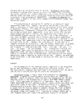 colonies. Subsequently, dark brown lesions appeared on the lower stems. From
August to September the effects were more acute and resulted in the complete
browning and death of entire aquatic plant beds. Although Bourn and Jenkins
(1928) found that increased salinity between 2 and 7 ppt lowered plant resis-
tance, Lumsden et al. (1963) found salinity inhibitory to R,. solani at 4 to 6
ppt. Studies with water hyacinth revealed increased susceptibility at 28 C
which decreased at 30 C or above (Joyner and Freeman 1973).
Rhizoctonia solani has been found to attack the majority of the species
of duck food plants with Potamogeton pectinatus being the most susceptible.
Vallisneria and Najas are not readily infected unless associated with
Potamogeton. Ruppia maritima was found to be the most susceptible next to
Potamogeton but usually survived infestation due to its reproductive powers.
Susceptibility generally decreased when plants grew in sandy soil somewhat
sheltered from the winds (Bourn and Jenkins 1928).
The 1961 blight of Potamogeton pectinatus in North Carolina was found to
result less from the presence of R_. solani and more from combined environmental
factors along with one or more Phythutm species. Three unidentified Phythium
species were determined with Phythium-3 being the most likely infectious agent.
Areas of higher salinity resulted in improved plant condition, however this
increased resistance to disease infection could have been the result of more
favorable environmental conditions for the plants (Lumsden et al. 1963).
Prior to 1963, Myrigphyl1 urn spicatum inhabitated over 40,000 ha in the
Chesapeake Bay (Elser 1969).ITs subsequent decline has been attributed to
Lake Venice Disease and/or Northeast Disease whose responsible pathogens have
yet to be isolated. Elser's study revealed that by 1967 healthy milfoil was
nowhere to be found in Maryland with most beds showing symptoms of both
diseases.
Lake Venice Disease manifests itself as a brownish, silt-like coating on
leaves and stems that causes a gradual wasting away of the host. If flowering
occurs, it is very sparse (Elser 1969). Only under low light intensities
(indirect light) in the labortory well plants produce symptoms resembling Lake
Venice Disease, and the disease cannot be mechanically transmitted (Bean
et al. 1973). Bean et al. concluded that only after low light intensity ex-
posure does Myriophyllum become susceptible to Lake Venice Disease. The casual
agent may be a bacterium, virus or fungi.
The Northeast Disease which attacks milfoil was extensively researched
by Bayley et al. (1968) who concluded that the disease was a virus, virus-like
particle or a toxin. Dr. K. Corbett (Virologist, University of Maryland) has
suggested that a causal agent may not exist, but rather the disease is a
result of a combination of environmental conditions (personal communication).
The Northeast Disease symptoms are: initially broken leaflets; stems and leaves
turn dark brownish green and become stiff; and the leaves gradually drop off
leaving a blackened stem. Distortion of the petioles is commonly seen when the
diesease progresses slowly (Elser 1969).
243
image:
colonies. Subsequently, dark brown lesions appeared on the lower stems. From
August to September the effects were more acute and resulted in the complete
browning and death of entire aquatic plant beds. Although Bourn and Jenkins
(1928) found that increased salinity between 2 and 7 ppt lowered plant resis-
tance, Lumsden et al. (1963) found salinity inhibitory to R,. solani at 4 to 6
ppt. Studies with water hyacinth revealed increased susceptibility at 28 C
which decreased at 30 C or above (Joyner and Freeman 1973).
Rhizoctonia solani has been found to attack the majority of the species
of duck food plants with Potamogeton pectinatus being the most susceptible.
Vallisneria and Najas are not readily infected unless associated with
Potamogeton. Ruppia maritima was found to be the most susceptible next to
Potamogeton but usually survived infestation due to its reproductive powers.
Susceptibility generally decreased when plants grew in sandy soil somewhat
sheltered from the winds (Bourn and Jenkins 1928).
The 1961 blight of Potamogeton pectinatus in North Carolina was found to
result less from the presence of R_. solani and more from combined environmental
factors along with one or more Phythutm species. Three unidentified Phythium
species were determined with Phythium-3 being the most likely infectious agent.
Areas of higher salinity resulted in improved plant condition, however this
increased resistance to disease infection could have been the result of more
favorable environmental conditions for the plants (Lumsden et al. 1963).
Prior to 1963, Myrigphyl1 urn spicatum inhabitated over 40,000 ha in the
Chesapeake Bay (Elser 1969).ITs subsequent decline has been attributed to
Lake Venice Disease and/or Northeast Disease whose responsible pathogens have
yet to be isolated. Elser's study revealed that by 1967 healthy milfoil was
nowhere to be found in Maryland with most beds showing symptoms of both
diseases.
Lake Venice Disease manifests itself as a brownish, silt-like coating on
leaves and stems that causes a gradual wasting away of the host. If flowering
occurs, it is very sparse (Elser 1969). Only under low light intensities
(indirect light) in the labortory well plants produce symptoms resembling Lake
Venice Disease, and the disease cannot be mechanically transmitted (Bean
et al. 1973). Bean et al. concluded that only after low light intensity ex-
posure does Myriophyllum become susceptible to Lake Venice Disease. The casual
agent may be a bacterium, virus or fungi.
The Northeast Disease which attacks milfoil was extensively researched
by Bayley et al. (1968) who concluded that the disease was a virus, virus-like
particle or a toxin. Dr. K. Corbett (Virologist, University of Maryland) has
suggested that a causal agent may not exist, but rather the disease is a
result of a combination of environmental conditions (personal communication).
The Northeast Disease symptoms are: initially broken leaflets; stems and leaves
turn dark brownish green and become stiff; and the leaves gradually drop off
leaving a blackened stem. Distortion of the petioles is commonly seen when the
diesease progresses slowly (Elser 1969).
243
image:
 Prolific growths of Zostera marina were characteristic of the Atlantic
Coast of the northern United States and Canada prior to 1931. At the same
time the West Coast of the United States and European Zostera beds were also
dimishing in size. Local declines were noticed as early as 1930. A devasting
disease which has inconclusively been attributed to Labyrinthula microcystis
almost completely destroyed the Zostera beds over much of the Atlantic Coast of
the United States from Beaufort, North Carolina to Nova Scotia by 1932 (Tutin
1934; Mackin unpublished). Destruction of the eelgrass beds resulted in the
washing away and erosion of previously bound sediments changing their con-
figuration and productivity (Linduska 1964). The disease has been described
as "epiphytotic" and "enphytotic" for various areas. In recent years, some
recovery has occurred both in the United States and Europe (Mackin unpublished).
The infection is not usually visible on new tissue, however, older leaves
display dark splotching and/or black lower leaves. Although usually confined
to the leaf epidermis, spotting may occur in any green tissue. Streaking is
the result of the infection of the larger, longitudinal mesophyll cells ending
at the lateral septa. The stem cuticle, cortex and rhizomes may also become
darkly discolored (Renn 1935; Tutin 1934).
According to Young (1943) the predominant morphological stage is the neo-
plasmodium. In this stage masses of filaments form an "intricate lacy network"
on which tapering cell bodies migrate singly or in "rope-like aggregates".
Sprus and vegetative cyst formationisa characteristic form in which the disease
is believed to be transported by water currents (Mackin unpublished). The
mechanism of motion is unknown, but the spindles produce filamentous pathways
on which the organisms seem to glide. Apparently, nutrition is obtained
through extracellular digestion and absorption in solution (Young 1943).
Labyrinthula has been found to be extremely tolerant of its environment.
Activity occurs in a range from 0.3 to 27 C, but the optimum temperature appears
to be between 14 and 24 C. This optimum correlates with the fructification of
Zostera,blighting it just prior to propagation. The pH tolerance ranges from
4 to 9 without great alteration of the organism's activity. Roughly the
salinity optimum is from just below seawater to quite a bit above it. The
temperature and salinity preferences are similar to the conditions prevalent
during the recorded periods of massive infestation during the summer months.
Additional hosts which are generally closely associated with eelgrass beds
include: two algae, Cladophora hirta and Chaetomorpha spp. Linum; and
Zannichellia palustris var major and Ruppia maritima var. rostrata (Young 1943).
Mackin_(unpublished) also cites Fucus furcatus, Ectocarpus conferoides,
Cystociom'um perpureum (all algae^ and Zostera hornemanniana. This wide host
range could insure the continued presence of Labyrinthula (Young 1943).
Another suggested causative agent for the disappearance of Zostera is the
fungus Qphiobolus halimus. Its abundance and activity is variable, especially
in the United States, and is not necessarily found in areas diseased by
Labyrinthula (Renn 1935). Mackin (unpublished) stated that its importance
in the wasting disease of eelgrass in the United States was improbable since it
was so rarely found. Renn (1934) restricted Ophiobolus effects to Canada and
northern Europe.
244
image:
Prolific growths of Zostera marina were characteristic of the Atlantic
Coast of the northern United States and Canada prior to 1931. At the same
time the West Coast of the United States and European Zostera beds were also
dimishing in size. Local declines were noticed as early as 1930. A devasting
disease which has inconclusively been attributed to Labyrinthula microcystis
almost completely destroyed the Zostera beds over much of the Atlantic Coast of
the United States from Beaufort, North Carolina to Nova Scotia by 1932 (Tutin
1934; Mackin unpublished). Destruction of the eelgrass beds resulted in the
washing away and erosion of previously bound sediments changing their con-
figuration and productivity (Linduska 1964). The disease has been described
as "epiphytotic" and "enphytotic" for various areas. In recent years, some
recovery has occurred both in the United States and Europe (Mackin unpublished).
The infection is not usually visible on new tissue, however, older leaves
display dark splotching and/or black lower leaves. Although usually confined
to the leaf epidermis, spotting may occur in any green tissue. Streaking is
the result of the infection of the larger, longitudinal mesophyll cells ending
at the lateral septa. The stem cuticle, cortex and rhizomes may also become
darkly discolored (Renn 1935; Tutin 1934).
According to Young (1943) the predominant morphological stage is the neo-
plasmodium. In this stage masses of filaments form an "intricate lacy network"
on which tapering cell bodies migrate singly or in "rope-like aggregates".
Sprus and vegetative cyst formationisa characteristic form in which the disease
is believed to be transported by water currents (Mackin unpublished). The
mechanism of motion is unknown, but the spindles produce filamentous pathways
on which the organisms seem to glide. Apparently, nutrition is obtained
through extracellular digestion and absorption in solution (Young 1943).
Labyrinthula has been found to be extremely tolerant of its environment.
Activity occurs in a range from 0.3 to 27 C, but the optimum temperature appears
to be between 14 and 24 C. This optimum correlates with the fructification of
Zostera,blighting it just prior to propagation. The pH tolerance ranges from
4 to 9 without great alteration of the organism's activity. Roughly the
salinity optimum is from just below seawater to quite a bit above it. The
temperature and salinity preferences are similar to the conditions prevalent
during the recorded periods of massive infestation during the summer months.
Additional hosts which are generally closely associated with eelgrass beds
include: two algae, Cladophora hirta and Chaetomorpha spp. Linum; and
Zannichellia palustris var major and Ruppia maritima var. rostrata (Young 1943).
Mackin_(unpublished) also cites Fucus furcatus, Ectocarpus conferoides,
Cystociom'um perpureum (all algae^ and Zostera hornemanniana. This wide host
range could insure the continued presence of Labyrinthula (Young 1943).
Another suggested causative agent for the disappearance of Zostera is the
fungus Qphiobolus halimus. Its abundance and activity is variable, especially
in the United States, and is not necessarily found in areas diseased by
Labyrinthula (Renn 1935). Mackin (unpublished) stated that its importance
in the wasting disease of eelgrass in the United States was improbable since it
was so rarely found. Renn (1934) restricted Ophiobolus effects to Canada and
northern Europe.
244
image:
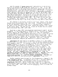 A considerable amount of controversy exists over the causative agent(s)
for the disappearance of Zostera marina. Labyrinthula has not been conslusive-
ly determined as the causative agent and Qphiobolus has been almost eliminated
from consideration. The salinity and temperature fluctuations have also been
considered for the decline. Butcher (1935, p. 545.) summed up the situation by
concluding that the disappearance of Zostera was more than likely due to a
"large number of circumstances and not...a single catastrophic event".
Elevated temperatures can result in a sub-optimal physiological condition
enabling opportunistic pathogenic organisms to overcome their hosts. Since
many pathogenic organisms are ubiquitous and constant components of the aquatic
environment, the development of stress conditions, i.e. elevated temperatures,
can result in infection perhaps leading to significant declines in areas af-
fected by thermal plumes (Mihursky et al. 1970).
Field observations in the 1970s have not indicated any recurring disease-
like symptoms on SAV. In the summer of 1977, Suzanne Bayley examined an ex-
tensive bed of Myriophyllum which looked brownish, but concluded it was not
diseased. R&ther the brown film on the leaves and stems was a mixture of
periphyton, detritus and sediment. The involvement of SAV as a group in recent
declines would seem to indicate that disease alone has not been responsible.
The likelihood is small that all the species in the Bay could be hit by a
single pathogenic species. It is possible that some major ecological change
could have resulted in the lowering of plant resistance thus allowing invasion
by a pathogen or series of pathogens. This environmental change could have
been one or more of such factors as turbidity, chlorine or agro-chemicals.
LOCAL ECOLOGICAL FACTORS
There are several environmental factors that negatively impact submerged
macrophytes on a localized level. Included among these are dredging and boat
traffic. Direct action from these sources can cause uprooting and physical
damage to grass beds. However, indirect impacts can be caused by the reintro-
duction of bottom sediments into the water column thus increasing turbidity.
The degree of impact from suspended sediments is related to bottom sediment
composition. Fine, silty organic materials require more time to settle out
than heavier, sandy material.
Dredging
A hydraulic clam dredge, for example, uproots all vegetation in a 75 to
90 cm wide paith. This apparently happended at the north side of Cambridge
Bridge on the Choptank in the 1960s. In very shallow water, boat pro-
pellers also uproot SAV. The extent and permanency of damage to SAV beds
depends on the reproductive means of the species involved. Species that
normally reproduce only sexually could be virtually wiped out by extensive
dredging. Species capable of vegetative reproduction have better chances for
survival.
245
image:
A considerable amount of controversy exists over the causative agent(s)
for the disappearance of Zostera marina. Labyrinthula has not been conslusive-
ly determined as the causative agent and Qphiobolus has been almost eliminated
from consideration. The salinity and temperature fluctuations have also been
considered for the decline. Butcher (1935, p. 545.) summed up the situation by
concluding that the disappearance of Zostera was more than likely due to a
"large number of circumstances and not...a single catastrophic event".
Elevated temperatures can result in a sub-optimal physiological condition
enabling opportunistic pathogenic organisms to overcome their hosts. Since
many pathogenic organisms are ubiquitous and constant components of the aquatic
environment, the development of stress conditions, i.e. elevated temperatures,
can result in infection perhaps leading to significant declines in areas af-
fected by thermal plumes (Mihursky et al. 1970).
Field observations in the 1970s have not indicated any recurring disease-
like symptoms on SAV. In the summer of 1977, Suzanne Bayley examined an ex-
tensive bed of Myriophyllum which looked brownish, but concluded it was not
diseased. R&ther the brown film on the leaves and stems was a mixture of
periphyton, detritus and sediment. The involvement of SAV as a group in recent
declines would seem to indicate that disease alone has not been responsible.
The likelihood is small that all the species in the Bay could be hit by a
single pathogenic species. It is possible that some major ecological change
could have resulted in the lowering of plant resistance thus allowing invasion
by a pathogen or series of pathogens. This environmental change could have
been one or more of such factors as turbidity, chlorine or agro-chemicals.
LOCAL ECOLOGICAL FACTORS
There are several environmental factors that negatively impact submerged
macrophytes on a localized level. Included among these are dredging and boat
traffic. Direct action from these sources can cause uprooting and physical
damage to grass beds. However, indirect impacts can be caused by the reintro-
duction of bottom sediments into the water column thus increasing turbidity.
The degree of impact from suspended sediments is related to bottom sediment
composition. Fine, silty organic materials require more time to settle out
than heavier, sandy material.
Dredging
A hydraulic clam dredge, for example, uproots all vegetation in a 75 to
90 cm wide paith. This apparently happended at the north side of Cambridge
Bridge on the Choptank in the 1960s. In very shallow water, boat pro-
pellers also uproot SAV. The extent and permanency of damage to SAV beds
depends on the reproductive means of the species involved. Species that
normally reproduce only sexually could be virtually wiped out by extensive
dredging. Species capable of vegetative reproduction have better chances for
survival.
245
image:
 Manning (1965) discussed experiments conducted in the Patuxent River and
the Eastern Bay in 1956 to determine revegetation requirements for areas
stripped of vegetation by clam dredges. In comparing two sections of the
Patuxent River, one area where thousands of bushels of clams had been dredged
and another area where dredging was prohibited, the conclusion was reached
that natural forces and conditions were responsible for SAV distribution and
abundance rather than clam dredging. No long term impacts from dredging
activities could be proved since the prohibited area showed less vegetation
than the dredged one.
Dredging for the purpose of increasing ambient depths completely removes
existing vegetation and alters the habitat. Macrophytes normally colonize
the shallower areas along the shoreline and extend out into deeper water based
on the photic zone. By increasing the depth, SAV would be prohibited from
recolonizing due to a decrease in the amount of light reaching the new dredged
bottom depth. However, dredging results in piece-meal destruction of a local-
ized nature rather than in Bay-wide impacts.
Boat Traffic
Damage to submerged macrophytes from boat propellers is essentially of
local importance. However, with the increased number of pleasure boats that
presently navigate the shallow water areas of the Chesapeake Bay estuary,
damage to existing beds could be considered to be more extensive.
Figure 15 (Chapter 1) shows an aerial photograph of an eelgrass bed in
Mobjack Bay, Virginia, that has been impacted by boating activity. The
crisscrossing pattern of light streaks indicates boat propeller damage. This
destruction is usually seasonal but excessive propeller disturbance over an ex-
tended period of time would continue to limit SAV on a localized basis.
WATER MOVEMENT - TIDES AND CURRENTS
Submerged aquatic species do not normally colonize areas subject to
continuous strong currents or tides. Excessive water movement tends to scour
the bottom to such an extent that submerged macrophytes are prohibited from
colonizing. Such water movement also resuspends fine sediment particles and
contributes towards increased turbidity.
Daily tidal flushing is necessary within an estuary in order to remove
metabolites and bring in nutrients. This was thought by Teal (1962) to be
responsible for the high productivities in a tidal salt marsh and was found
necessary for aquatic plant community development in the South River (Philipp
and Brown 1965). Submerged plants are exposed to daily variations in light
quality and quantity as a result of tidal currents. In .extremes this can be
detrimental' (Joanen and Glasgow 1965). Extreme low tides cause plants to
become exposed resulting in dessication. Extreme high tides raise ambient
water depths and effectively decrease light penetration to the benthos.
246
image:
Manning (1965) discussed experiments conducted in the Patuxent River and
the Eastern Bay in 1956 to determine revegetation requirements for areas
stripped of vegetation by clam dredges. In comparing two sections of the
Patuxent River, one area where thousands of bushels of clams had been dredged
and another area where dredging was prohibited, the conclusion was reached
that natural forces and conditions were responsible for SAV distribution and
abundance rather than clam dredging. No long term impacts from dredging
activities could be proved since the prohibited area showed less vegetation
than the dredged one.
Dredging for the purpose of increasing ambient depths completely removes
existing vegetation and alters the habitat. Macrophytes normally colonize
the shallower areas along the shoreline and extend out into deeper water based
on the photic zone. By increasing the depth, SAV would be prohibited from
recolonizing due to a decrease in the amount of light reaching the new dredged
bottom depth. However, dredging results in piece-meal destruction of a local-
ized nature rather than in Bay-wide impacts.
Boat Traffic
Damage to submerged macrophytes from boat propellers is essentially of
local importance. However, with the increased number of pleasure boats that
presently navigate the shallow water areas of the Chesapeake Bay estuary,
damage to existing beds could be considered to be more extensive.
Figure 15 (Chapter 1) shows an aerial photograph of an eelgrass bed in
Mobjack Bay, Virginia, that has been impacted by boating activity. The
crisscrossing pattern of light streaks indicates boat propeller damage. This
destruction is usually seasonal but excessive propeller disturbance over an ex-
tended period of time would continue to limit SAV on a localized basis.
WATER MOVEMENT - TIDES AND CURRENTS
Submerged aquatic species do not normally colonize areas subject to
continuous strong currents or tides. Excessive water movement tends to scour
the bottom to such an extent that submerged macrophytes are prohibited from
colonizing. Such water movement also resuspends fine sediment particles and
contributes towards increased turbidity.
Daily tidal flushing is necessary within an estuary in order to remove
metabolites and bring in nutrients. This was thought by Teal (1962) to be
responsible for the high productivities in a tidal salt marsh and was found
necessary for aquatic plant community development in the South River (Philipp
and Brown 1965). Submerged plants are exposed to daily variations in light
quality and quantity as a result of tidal currents. In .extremes this can be
detrimental' (Joanen and Glasgow 1965). Extreme low tides cause plants to
become exposed resulting in dessication. Extreme high tides raise ambient
water depths and effectively decrease light penetration to the benthos.
246
image:
 However, a scan of tide records from the Chesapeake Biological Laboratory
at Solomons, Maryland did not show any abnormal tide events which did not also
occur in previous decades. Therefore, this can be safely ruled out as a major
factor in the SAV declines of the 1970s.
Extreme water movement resulting from storm events can cause substantial
physical damage to existing aquatic beds. Field observations by McCann (1945)
determined that the branch tops at the surface are often fractured by wave
action. In the case of Ruppia maritima, these detached fragments are not
capable of survival. Such storm events as Agnes in 1972 and Eloise in 1975
may have negatively impacted Bay submerged vegetation; however, historic
accounts of previous major storm events do not indicate vegetation losses
from storm damage alone. This is probable because submerged aquatics can
quickly colonize areas by vegetative reproduction (see Chapter 1). Thus
physical disturbance is a stress factor which these plants are well adapted to.
PH
As discussed in Chapter 2, the photosynthesis and respiratory activity of
submerged aquatic flora causes diurnal fluctuations in the dissolved C02 content
of an aquatic environment. pH, in turn, affects plant enzyme activity, seed
germination and variety of other plant responses.
The normal pH of the Chesapeake Bay is from about 6 to 9. Drastic fluct-
uations could cause damage to SAV; however, given an otherwise favorable en-
vironment and sufficient necessary nutrients, most SAV species should be able
to tolerate a wide pH range. Extreme pH fluctuations can probably be found
as a localized condition resulting from industrial effluent input. Such a
situation would be of a point source nature and would affect native vegetation
only in the immediate vicinity of the effluent sources. No documentation
has been found as to whethkr pH fluctuations have affected SAV in the Chesapeake
Bay.
CARBON DIOXIDE SOURCES
Submerged aquatic species have potentially three entry ports for the C02
necessary for photosynthesis. Aquatic plants are capable of utilizing dis-
solved C02 in the water column through leaf uptake. They are also able to take
up bicarbonate ion (HC03~) for usage, and finally CO may possible be taken up
from the sediments by the roots and transported to the leaves. These three
possibilities are of interest because they furnish the most crucial raw material
for photosynthesis in the stuarine environment—carbon. Any limitation in the
carbon availability would be reflected in an intermediate decline of SAV pro-
ductivity. The problem is that carbon dioxide dissolved in water has a much
lower coefficient of molecular diffusion than under gaseous conditions. This
situation is complicated by the existence of a boundary layer of unstirred water
near the surfaces of SAV leaves (Gessner 1955, cited in Sculthorpe 1967).
These physical conditions lead to a very slow entry rate of CO into aquatic
plants compared to land plants under the same concentrations of free C02.
247
image:
However, a scan of tide records from the Chesapeake Biological Laboratory
at Solomons, Maryland did not show any abnormal tide events which did not also
occur in previous decades. Therefore, this can be safely ruled out as a major
factor in the SAV declines of the 1970s.
Extreme water movement resulting from storm events can cause substantial
physical damage to existing aquatic beds. Field observations by McCann (1945)
determined that the branch tops at the surface are often fractured by wave
action. In the case of Ruppia maritima, these detached fragments are not
capable of survival. Such storm events as Agnes in 1972 and Eloise in 1975
may have negatively impacted Bay submerged vegetation; however, historic
accounts of previous major storm events do not indicate vegetation losses
from storm damage alone. This is probable because submerged aquatics can
quickly colonize areas by vegetative reproduction (see Chapter 1). Thus
physical disturbance is a stress factor which these plants are well adapted to.
PH
As discussed in Chapter 2, the photosynthesis and respiratory activity of
submerged aquatic flora causes diurnal fluctuations in the dissolved C02 content
of an aquatic environment. pH, in turn, affects plant enzyme activity, seed
germination and variety of other plant responses.
The normal pH of the Chesapeake Bay is from about 6 to 9. Drastic fluct-
uations could cause damage to SAV; however, given an otherwise favorable en-
vironment and sufficient necessary nutrients, most SAV species should be able
to tolerate a wide pH range. Extreme pH fluctuations can probably be found
as a localized condition resulting from industrial effluent input. Such a
situation would be of a point source nature and would affect native vegetation
only in the immediate vicinity of the effluent sources. No documentation
has been found as to whethkr pH fluctuations have affected SAV in the Chesapeake
Bay.
CARBON DIOXIDE SOURCES
Submerged aquatic species have potentially three entry ports for the C02
necessary for photosynthesis. Aquatic plants are capable of utilizing dis-
solved C02 in the water column through leaf uptake. They are also able to take
up bicarbonate ion (HC03~) for usage, and finally CO may possible be taken up
from the sediments by the roots and transported to the leaves. These three
possibilities are of interest because they furnish the most crucial raw material
for photosynthesis in the stuarine environment—carbon. Any limitation in the
carbon availability would be reflected in an intermediate decline of SAV pro-
ductivity. The problem is that carbon dioxide dissolved in water has a much
lower coefficient of molecular diffusion than under gaseous conditions. This
situation is complicated by the existence of a boundary layer of unstirred water
near the surfaces of SAV leaves (Gessner 1955, cited in Sculthorpe 1967).
These physical conditions lead to a very slow entry rate of CO into aquatic
plants compared to land plants under the same concentrations of free C02.
247
image:
 This limited accessibility has given an evolutionary advantage to those species
which maximize surface area for absorption of COa- Dissolved C02 appears to be
the preferred carbon source for submerged aquatic vegetation (Steeman Nielson
1946).
It has long been speculated and argued that aquatic plants possess the
ability to utilize bicarbonate ions for subsequent use in the Calvin cycle. A
historical review on the subject is presented by Sculthorpe (1967). Hutchinson
(1975), in a synthesis of the various experiments performed in this regard,
concluded that of the flowering aquatic plants which occur in the Chesapeake Bay,
the following can use bicarbonate as a source of carbon: Ceratophyllurn demersum,
Myriophyllum s pica turn, Vallisneria sjn'ralis. Elodea canadensis and Potamogeton
pectinatus. The selective advantage that this ability confers is significant.
When the pH rises above 9.0, free carbon dioxide does not exist, and plants
existing at levels higher than this would have to be able to use HC03~.
Assimilation in more'acid conditions could occur, even if the CCh levels were
removed to a point of depletion. In most aqueous systems, the concentration
of HC03~ is likely to be several times and in some cases several hundred times
the concentrations of C02. The advantage of being able to draw on this reserve
in periods of low dissolved C02 is obvious.
Bicarbonate ions are taken up through both sides of the leaf of Potamogeton
as the calcium salt. This uptake is balanced by the release of Ca(OH)a through
the upper surfaces, and the reaction is light dependent (Hutchinson 1975). The
uptake mechanism and subsequent usage of bicarbonate can be thought of as a
rough aquatic analog to the 4-carbon Hatch-Slack pathway evident in some
terrestrial species. Carbon dioxide in both cases is complexed with a "carrier"
compound and actively transported to a location where decarboxylation can occur
and C02 entered into the Calvin cycle. The chemical nature of the carrier in
aquatic species is unclear at this time.
Wiurn-Anderson (1971) working with an aquatic genus not covered by this
volume, Lobelia, has determined that root uptake of C02 occurs followed by
trans!ocation to the photosynthetic site. That this occurs in other macrophytes
has not been determined, however, a suggestion of this is seen by Hutchinson
(1975) in the presence of many chloroplasts in the cells surrounding air spaces
in the submerged stems of Myriophyllum. This pathway may be significant in
environmental situations where C02 levels in the water column are low and those
in the sediments high.
Submerged aquatic vegetation may be carbon limited under certain environ-
mental conditions. There is a close association in natural sea water between
salinity, pH and bicarbonate supply. A drop in salinity results in a pH drop
and a shift in carbon form away from bicarbonates and thus may limit photosyn-
thesis (Hammer 1968; Ogata and Matsui 1971). The shift in carbon source is
likely to be more of a limiting factor than the osmotic pressure differential
which also accompanies lowered salinity. Hammer (1968) maintained photosynthetic
levels while dropping salinity by the addition of biearberotes.
Changes in submerged vegetation patterns noticed in recent j^,^ „.-., 3s.
on carbon availability. Salinity in the Chesapeake Bay has decreased somewhat
ntly from an average of 15.441 ppt in 1971 to 8.487 ppt in
recent years may hinge
un Ldruun dVd i iduiiity. ocumiuy in uie uriebdpecn^e oay iias decreased somewhat
recently from an average of 15.441 ppt in 1971 to 8.487 ppt in 1976. Following
248
image:
This limited accessibility has given an evolutionary advantage to those species
which maximize surface area for absorption of COa- Dissolved C02 appears to be
the preferred carbon source for submerged aquatic vegetation (Steeman Nielson
1946).
It has long been speculated and argued that aquatic plants possess the
ability to utilize bicarbonate ions for subsequent use in the Calvin cycle. A
historical review on the subject is presented by Sculthorpe (1967). Hutchinson
(1975), in a synthesis of the various experiments performed in this regard,
concluded that of the flowering aquatic plants which occur in the Chesapeake Bay,
the following can use bicarbonate as a source of carbon: Ceratophyllurn demersum,
Myriophyllum s pica turn, Vallisneria sjn'ralis. Elodea canadensis and Potamogeton
pectinatus. The selective advantage that this ability confers is significant.
When the pH rises above 9.0, free carbon dioxide does not exist, and plants
existing at levels higher than this would have to be able to use HC03~.
Assimilation in more'acid conditions could occur, even if the CCh levels were
removed to a point of depletion. In most aqueous systems, the concentration
of HC03~ is likely to be several times and in some cases several hundred times
the concentrations of C02. The advantage of being able to draw on this reserve
in periods of low dissolved C02 is obvious.
Bicarbonate ions are taken up through both sides of the leaf of Potamogeton
as the calcium salt. This uptake is balanced by the release of Ca(OH)a through
the upper surfaces, and the reaction is light dependent (Hutchinson 1975). The
uptake mechanism and subsequent usage of bicarbonate can be thought of as a
rough aquatic analog to the 4-carbon Hatch-Slack pathway evident in some
terrestrial species. Carbon dioxide in both cases is complexed with a "carrier"
compound and actively transported to a location where decarboxylation can occur
and C02 entered into the Calvin cycle. The chemical nature of the carrier in
aquatic species is unclear at this time.
Wiurn-Anderson (1971) working with an aquatic genus not covered by this
volume, Lobelia, has determined that root uptake of C02 occurs followed by
trans!ocation to the photosynthetic site. That this occurs in other macrophytes
has not been determined, however, a suggestion of this is seen by Hutchinson
(1975) in the presence of many chloroplasts in the cells surrounding air spaces
in the submerged stems of Myriophyllum. This pathway may be significant in
environmental situations where C02 levels in the water column are low and those
in the sediments high.
Submerged aquatic vegetation may be carbon limited under certain environ-
mental conditions. There is a close association in natural sea water between
salinity, pH and bicarbonate supply. A drop in salinity results in a pH drop
and a shift in carbon form away from bicarbonates and thus may limit photosyn-
thesis (Hammer 1968; Ogata and Matsui 1971). The shift in carbon source is
likely to be more of a limiting factor than the osmotic pressure differential
which also accompanies lowered salinity. Hammer (1968) maintained photosynthetic
levels while dropping salinity by the addition of biearberotes.
Changes in submerged vegetation patterns noticed in recent j^,^ „.-., 3s.
on carbon availability. Salinity in the Chesapeake Bay has decreased somewhat
ntly from an average of 15.441 ppt in 1971 to 8.487 ppt in
recent years may hinge
un Ldruun dVd i iduiiity. ocumiuy in uie uriebdpecn^e oay iias decreased somewhat
recently from an average of 15.441 ppt in 1971 to 8.487 ppt in 1976. Following
248
image:
 the argument presented above, the carbon balance has then been shifted in favor
of C02- Qrth (unpublished) believes temperature to be an important factor in
the decline of SAV. The rise in temperature he has noted would decrease the
solubility of C02 thus making it less accessible to macrophyte species. Nutrient
inputs could ehnance algal species that, because of their favorable surface
to volume ratio, could compete effectively with aquatic macrophytes for
available C02. More research involving carbonate levels needs to be done to
determine the relative importance of this factor in assessing SAV declines.
HEAVY METALS
Heavy metals occur naturally in marine, brackish and fresh waters generally
in increasing concentrations with decreasing salinity (Bureau of Land Management
1976). Table 83 lists various common heavy metals with estimated values of
natural occurrence in marine and fresh waters. Higher values in estuarine
waters result from man-oriented sources as point and nonpoint pollution such as
municipal wastes, industrial effluents, agricultural drainage and petrochemical
products (Schroeder 1977; Sculthorpe 1967; Bureau of Land Management 1976).
Heavy metals generally are resistant to biological or chemical degradation
(Bureau of Land Management 1976). Once introduced into an aquatic medium,
soluble heavy metals tend to become adsorbed, complexed or precipitated onto
particulates. Adsorption may occur not only to sediment particles but also to
phytoplankton (Schroeder 1977). Not all metals are adsorbed equally nor are
heavy metals associated solely with particulates. Small amounts of heavy metals
can remain in solution (Bureau of Land Management 1976).
The role of heavy metals in plant metabolism is not fully understood. Some
relationships, however, have been established. For instance, iron appears to
be necessary for chlorophyll synthesis; manganese is essential for respiration
and nitrogen metabolism; copper is an important enzyme component; and zinc is
involved in auxin synthesis (Devlin 1975).
The normal uptake of heavy metals by submerged aquatic vegetation frequently
results in element concentration in plant tissue. Hutchinson (1975) cites the
work of numerous scientists substantiating the concentration of vanadium, copper
and zinc by P. pectinatus, copper and zinc by Vallisneria sp. and copper by
Chara sp. Both El odea and Myriophyllum spicaturn were found to concentrate iron.
Ceratophyllum demersum has been tested extensively for metal concentrations and
found to accumulate copper, zinc and chromium. Concentration factor ratios of
element concentration in organism to element concentration in environment have
been documented in Ceratophyllum demersum for arsenic (1,100 to 1,700 ppm),
cadmium (500 to 700 ppm) and mercury (about 70 ppm). Experiments with Zostera
marina in Alaska (Bureau of Land Management 1976), have shown that zinc, copper
and cadmium can become concentrated in roots, rhizomes and leaves.
It has been previously established that SAV plays an essential role in the
food web through consumption of live material and detritus by herbivores and
filter feeders (see Chapter 2). Due to the ability to concentrate heavy metals,
SAV can serve as a vehicle for the recycling of heavy metals to higher trophic
levels. This can result in increased and possibly toxic levels of heavy metals
249
image:
the argument presented above, the carbon balance has then been shifted in favor
of C02- Qrth (unpublished) believes temperature to be an important factor in
the decline of SAV. The rise in temperature he has noted would decrease the
solubility of C02 thus making it less accessible to macrophyte species. Nutrient
inputs could ehnance algal species that, because of their favorable surface
to volume ratio, could compete effectively with aquatic macrophytes for
available C02. More research involving carbonate levels needs to be done to
determine the relative importance of this factor in assessing SAV declines.
HEAVY METALS
Heavy metals occur naturally in marine, brackish and fresh waters generally
in increasing concentrations with decreasing salinity (Bureau of Land Management
1976). Table 83 lists various common heavy metals with estimated values of
natural occurrence in marine and fresh waters. Higher values in estuarine
waters result from man-oriented sources as point and nonpoint pollution such as
municipal wastes, industrial effluents, agricultural drainage and petrochemical
products (Schroeder 1977; Sculthorpe 1967; Bureau of Land Management 1976).
Heavy metals generally are resistant to biological or chemical degradation
(Bureau of Land Management 1976). Once introduced into an aquatic medium,
soluble heavy metals tend to become adsorbed, complexed or precipitated onto
particulates. Adsorption may occur not only to sediment particles but also to
phytoplankton (Schroeder 1977). Not all metals are adsorbed equally nor are
heavy metals associated solely with particulates. Small amounts of heavy metals
can remain in solution (Bureau of Land Management 1976).
The role of heavy metals in plant metabolism is not fully understood. Some
relationships, however, have been established. For instance, iron appears to
be necessary for chlorophyll synthesis; manganese is essential for respiration
and nitrogen metabolism; copper is an important enzyme component; and zinc is
involved in auxin synthesis (Devlin 1975).
The normal uptake of heavy metals by submerged aquatic vegetation frequently
results in element concentration in plant tissue. Hutchinson (1975) cites the
work of numerous scientists substantiating the concentration of vanadium, copper
and zinc by P. pectinatus, copper and zinc by Vallisneria sp. and copper by
Chara sp. Both El odea and Myriophyllum spicaturn were found to concentrate iron.
Ceratophyllum demersum has been tested extensively for metal concentrations and
found to accumulate copper, zinc and chromium. Concentration factor ratios of
element concentration in organism to element concentration in environment have
been documented in Ceratophyllum demersum for arsenic (1,100 to 1,700 ppm),
cadmium (500 to 700 ppm) and mercury (about 70 ppm). Experiments with Zostera
marina in Alaska (Bureau of Land Management 1976), have shown that zinc, copper
and cadmium can become concentrated in roots, rhizomes and leaves.
It has been previously established that SAV plays an essential role in the
food web through consumption of live material and detritus by herbivores and
filter feeders (see Chapter 2). Due to the ability to concentrate heavy metals,
SAV can serve as a vehicle for the recycling of heavy metals to higher trophic
levels. This can result in increased and possibly toxic levels of heavy metals
249
image:
 Table 83. Naturally occurring soluble concentrations of various heavy metals
in seawater and United States rivers
Concentrations Concentration ranges
in seawater in U. S. rivers
Element ppb
Brewer 1975 (cited in Schroeder 1977)
Kopp and Droner 1968;
Typical concentration
Mercury
Cadmium
Zinc
Copper
Nickel
Lead
Silver
Cobalt
Iron
Manganese
Chronium
0.03
0.1
4.9
0.5
1.7
0.03
0.04
0.05
2
0.2
0.3
<0.1 to 17
<0.1 to 80
1 to 800
0.9 to 12
0.3C
3C
0.1 to 0.55
0.037 to 0.44
< lc
<1 to 180
0.1 to 2.46
Kopp and Droner 1968; Turekian 1971 (cited in Schroeder 1977)
c
250
image:
Table 83. Naturally occurring soluble concentrations of various heavy metals
in seawater and United States rivers
Concentrations Concentration ranges
in seawater in U. S. rivers
Element ppb
Brewer 1975 (cited in Schroeder 1977)
Kopp and Droner 1968;
Typical concentration
Mercury
Cadmium
Zinc
Copper
Nickel
Lead
Silver
Cobalt
Iron
Manganese
Chronium
0.03
0.1
4.9
0.5
1.7
0.03
0.04
0.05
2
0.2
0.3
<0.1 to 17
<0.1 to 80
1 to 800
0.9 to 12
0.3C
3C
0.1 to 0.55
0.037 to 0.44
< lc
<1 to 180
0.1 to 2.46
Kopp and Droner 1968; Turekian 1971 (cited in Schroeder 1977)
c
250
image:
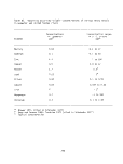 in aquatic fauna and man. However, without SAV to aid in recylcling metals,
bottom sediments in the vicinity of heavy metals input can become a metal sink
of sufficient toxicity to be unable to support any life (Davey and Phelps 1975),
Toxicity of heavy metals to species of submerged aquatics has not been
established. Hydroponic studies by Lee et al. (1976) determined that several
species of marsh plants were sensitive to heavy metals. They found that
levels of iron and phosphorus in plant roots were related to the accumulation
of zinc, nickel, lead and chromium. The absorption and translocation of
phosphorus may be influenced by heavy metals. Sensitivity to heavy metals may
also be greater in plants with a lower capacity to absorb and translocate iron.
Lee et al. concluded that phosphorus and iron levels in roots may serve as a
mechanism to control heavy metal levels.
Based on the lack of knowledge of the biological impacts of excessive
levels of heavy metals to SAV and the extent of heavy metal pollution in the
Chesapeake Bay, it is not possible to correlate recent SAV declines to metal
inputs. It is possible that Bay grasses may be accumulating heavy metals in
toxic or near toxic concentrations; however, there is no data available to
support or refute such a hypothesis.
PETROCHEMICALS
Increasing inputs of petrochemicals and petrochemical products into the
nation's waters have become a cause for concern. Petrochemicals enter the
aquatic environment from tankers, refineries, municipal and industrial
effluents, boats, and urban and river runoff. Despite the extravagance of
petroleum inputs from oil spills, an estimated 41.7 percent of the petroleum
products that reach marine environments come from urban and river runoff.
Farrington (1975) refers to this input as "chronic dribbling."
Rough estimates of annual petroleum inputs into the Chesapeake Bay
(U.S. Army Corps of Engineers 1977) indicate approximately 47 percent comes
from urban and river sources. Municipal and industrial sources account for
about 44 percent. These percentages are based on a total input of about
37,200 metric tons per year. The remaining petrochemical inputs consisted of
0.8 percent from oil spills, 1 percent from ship generated wastes and 8 percent
from boats.
Sediment sampling by the Annapolis Field Office of the U. S. Environmental
Protection Agency (U.S. Army Corps of Engineers 1977) found a range from
420 to 81,220 mg/kg oil and grease in Baltimore Harbor sediments. "Oil and
grease", as defined by EPA's laboratory analysis, included naturally occurring
lipids and hydrocarbons. Thus in order to differentiate between naturally
occurring and man induced oil and grease, EPA suggested that any oil and grease
concentrations in sediments greater than 1,000 to 1,500 mg/kg would probably
have resulted from petroleum contamination.
A study by the Chesapeake Bay Foundation (1977) concluded that from 1973
through 1976, 379,702 gallons of petroleum products entered the Bay from spills
in Maryland during transport and handling. Virginia contributed 497,391 gallons
251
image:
in aquatic fauna and man. However, without SAV to aid in recylcling metals,
bottom sediments in the vicinity of heavy metals input can become a metal sink
of sufficient toxicity to be unable to support any life (Davey and Phelps 1975),
Toxicity of heavy metals to species of submerged aquatics has not been
established. Hydroponic studies by Lee et al. (1976) determined that several
species of marsh plants were sensitive to heavy metals. They found that
levels of iron and phosphorus in plant roots were related to the accumulation
of zinc, nickel, lead and chromium. The absorption and translocation of
phosphorus may be influenced by heavy metals. Sensitivity to heavy metals may
also be greater in plants with a lower capacity to absorb and translocate iron.
Lee et al. concluded that phosphorus and iron levels in roots may serve as a
mechanism to control heavy metal levels.
Based on the lack of knowledge of the biological impacts of excessive
levels of heavy metals to SAV and the extent of heavy metal pollution in the
Chesapeake Bay, it is not possible to correlate recent SAV declines to metal
inputs. It is possible that Bay grasses may be accumulating heavy metals in
toxic or near toxic concentrations; however, there is no data available to
support or refute such a hypothesis.
PETROCHEMICALS
Increasing inputs of petrochemicals and petrochemical products into the
nation's waters have become a cause for concern. Petrochemicals enter the
aquatic environment from tankers, refineries, municipal and industrial
effluents, boats, and urban and river runoff. Despite the extravagance of
petroleum inputs from oil spills, an estimated 41.7 percent of the petroleum
products that reach marine environments come from urban and river runoff.
Farrington (1975) refers to this input as "chronic dribbling."
Rough estimates of annual petroleum inputs into the Chesapeake Bay
(U.S. Army Corps of Engineers 1977) indicate approximately 47 percent comes
from urban and river sources. Municipal and industrial sources account for
about 44 percent. These percentages are based on a total input of about
37,200 metric tons per year. The remaining petrochemical inputs consisted of
0.8 percent from oil spills, 1 percent from ship generated wastes and 8 percent
from boats.
Sediment sampling by the Annapolis Field Office of the U. S. Environmental
Protection Agency (U.S. Army Corps of Engineers 1977) found a range from
420 to 81,220 mg/kg oil and grease in Baltimore Harbor sediments. "Oil and
grease", as defined by EPA's laboratory analysis, included naturally occurring
lipids and hydrocarbons. Thus in order to differentiate between naturally
occurring and man induced oil and grease, EPA suggested that any oil and grease
concentrations in sediments greater than 1,000 to 1,500 mg/kg would probably
have resulted from petroleum contamination.
A study by the Chesapeake Bay Foundation (1977) concluded that from 1973
through 1976, 379,702 gallons of petroleum products entered the Bay from spills
in Maryland during transport and handling. Virginia contributed 497,391 gallons
251
image:
 from 1974 to 1976. Spills in Baltimore Harbor resulted in 40 percent of the
Maryland input and 50 percent of the Virginia contribution occurred in the
Elizabeth River.
Included in petroleum products are a number of different products:
kerosene, gasoline, crude oil and fuel oil contain "lower molecular weight
components" that evaporate quickly and are more soluble. Lubricating oils
contain heavier molecular weight components that are not readily evaporated.
Upon mixing with water and sediments, oil can be adsorbed directly onto sediments
or fractionated with some components subsequently adhereing to sediments.
Sediments are then available for resuspension and transportation (Farrington
1975).Crude oil contains thousands of compounds (Brown 1975). Some components
can be biodegraded by such organisms as bacteria of yeasts. However, the
impacts on marine organisms resulting from such microbial degradation are as
yet unknown (Farrington 1975).
The impact of oil contaminated sediments on submerged aquatic vegetation
appears to be largely unknown. Farrington (1975) suggested that marsh grasses
may be made unsuitable as a habitat. This could apply also to submerged
grasses. A further mode of impact to SAV could occur through the capacity of
oil and oil contaminated sediments to concentrate heavy metals and pesticides.
Brown (1975) cited Walker and Colwell (1974) and Seba and Corcoran (1969)
as having found an association between increased oil polluted sediments and
increased sediment concentrations of zinc, chromium, lead, copper, nickel,
cadmium and mercury, aldrin, dieldrin, DDT and possibly lindane, chlordane and
heptachlor expoxide.
Free oil may also coat vegetation and could impact SAV by physically
blocking nutrient assimilation and gas exchange in above bottom plant parts.
Cowell (1969) cited in Ecological Analysists, Inc. (1976) maintained that
oil can be directly toxic and even lethal to salt marsh flora. This may
also be true for submerged vegetation. Ecological Analysts, Inc. (1976)
suggested that negative impacts to annuals would probably be greater than
to perennials due to the capability of regrowth from rhizomes in perennial
species.
Based on the lack of knowledge of the biological impact of petrochemicals
and petrochemical products in an estuarine environment and the extent of oil
polluted sediments in the Chesapeake Bay, it is not possible to correlate
recent SAV declines with oil inputs. Extensive laboratory and field anlayses
would be required before such a correlation could be attempted.
SUMMARY
The previous chapter provided evidence to support the conclusion that
submerged aquatic vegetation in the Chesapeake Bay has declined over the past
40 years. Based on this conclusion, various environmental factors have been
investigated in order to ascertain possible causes for the Bay grass losses.
Factors that can negatively impact the aquatic environment are summarized on
two levels—localized impacts and Baywide impacts.
252
image:
from 1974 to 1976. Spills in Baltimore Harbor resulted in 40 percent of the
Maryland input and 50 percent of the Virginia contribution occurred in the
Elizabeth River.
Included in petroleum products are a number of different products:
kerosene, gasoline, crude oil and fuel oil contain "lower molecular weight
components" that evaporate quickly and are more soluble. Lubricating oils
contain heavier molecular weight components that are not readily evaporated.
Upon mixing with water and sediments, oil can be adsorbed directly onto sediments
or fractionated with some components subsequently adhereing to sediments.
Sediments are then available for resuspension and transportation (Farrington
1975).Crude oil contains thousands of compounds (Brown 1975). Some components
can be biodegraded by such organisms as bacteria of yeasts. However, the
impacts on marine organisms resulting from such microbial degradation are as
yet unknown (Farrington 1975).
The impact of oil contaminated sediments on submerged aquatic vegetation
appears to be largely unknown. Farrington (1975) suggested that marsh grasses
may be made unsuitable as a habitat. This could apply also to submerged
grasses. A further mode of impact to SAV could occur through the capacity of
oil and oil contaminated sediments to concentrate heavy metals and pesticides.
Brown (1975) cited Walker and Colwell (1974) and Seba and Corcoran (1969)
as having found an association between increased oil polluted sediments and
increased sediment concentrations of zinc, chromium, lead, copper, nickel,
cadmium and mercury, aldrin, dieldrin, DDT and possibly lindane, chlordane and
heptachlor expoxide.
Free oil may also coat vegetation and could impact SAV by physically
blocking nutrient assimilation and gas exchange in above bottom plant parts.
Cowell (1969) cited in Ecological Analysists, Inc. (1976) maintained that
oil can be directly toxic and even lethal to salt marsh flora. This may
also be true for submerged vegetation. Ecological Analysts, Inc. (1976)
suggested that negative impacts to annuals would probably be greater than
to perennials due to the capability of regrowth from rhizomes in perennial
species.
Based on the lack of knowledge of the biological impact of petrochemicals
and petrochemical products in an estuarine environment and the extent of oil
polluted sediments in the Chesapeake Bay, it is not possible to correlate
recent SAV declines with oil inputs. Extensive laboratory and field anlayses
would be required before such a correlation could be attempted.
SUMMARY
The previous chapter provided evidence to support the conclusion that
submerged aquatic vegetation in the Chesapeake Bay has declined over the past
40 years. Based on this conclusion, various environmental factors have been
investigated in order to ascertain possible causes for the Bay grass losses.
Factors that can negatively impact the aquatic environment are summarized on
two levels—localized impacts and Baywide impacts.
252
image:
 Localized impacts generally include turbidity, chlorine, nutrient loading,
boat activity and dredging. Turbidity, chlorine and nutrient loading, while
affecting more than one sub-estuary, have not been found applicable to the
entire Bay. Based on data from the late 1960s through the 1970s, a few areas
in the Bay have shown increases in turbidity, yet most have decreased. Chlorine
inputs into the Bay have risen along with increasing population in the Bay area.
There seems to be some evidence that excessive turbidities and chlorine plus
its by-products negatively impact SAV. However, experimental work is needed
to determine the extent of the effects. There is little evidence at this point
that chlorine has more than a localized impact, but research is presently in
progress.
Excessive nutrient loading often results in plankton and algal blooms such
as have been noted in the Potomac River. There is no evidence that such a
situation extends beyond parts of sub-estuaries. The main stem of the Bay has
high flushing rates, large size and good vertical mixing which give it a re-
latively high resiliency to sewage loadings from metropolitan point sources.
Power boats can cause localized impacts to SAV beds through propeller damage.
Dredging, whether for clams or for increasing water depths, effectively removes
SAV from the dredge line.
Impacts applicable on a Baywide scope generally include salinity, temper-
ature, HC03~j fauna, epiphytes, disease, agro-chemicals and large scale
weather events. The bicarbonate ion as a carbon source may be a factor in
plant declines in the lower saline areas of the Bay, but probably is not re-
levant in the lower Bay where higher salinities are found. In these higher
salinity areas, HC03~ is more readily available. Unfortunately little is
presently known concerning the importance of the bicarbonate ion to SAV.
Salinity has been implicated in the SAV problem. Over the past six years,
salinities in the Bay have decreased subsequent to a salinity increase observed
during the 1960s. Such a decrease as is presently being experienced might have
a slight impact on a species such as Zostera marina which thrives in high
salinities. Most other species actually prefer fresh water and brackish
situations and can easily tolerate salinity decreases.
Baywide impacts due to temperature are not supported by substantial evid-
ence. There are no indications that ambient temperatures have risen suffic-
iently to impact Bay grasses except in thermal plumes and possibly in the
lower Bay. There is also no evidence as to Baywide grass losses due to ex-
cessive faunal activity or epiphytic associations.
Investigations into the disease theory for SAV declines have determined
that specific species are susceptitble to several pathogenic organisms. How-
ever, during the years when Zostera marina was declining and Myriophyllum
spicatum was dying back, there was no indication that the involved "diseases"
were pathogenic to the many other SAV species native to the Chesapeake Bay.
The impact of agro-chemicals on SAV is presently under scrutiny. Herbi-
cide usage has increased heavily in the Bay area, yet an understanding of
the fate and mode of action of herbicides in an aquatic environment plus their
subsequent impact on SAV is not known. Herbicides, both dissolved and
253
image:
Localized impacts generally include turbidity, chlorine, nutrient loading,
boat activity and dredging. Turbidity, chlorine and nutrient loading, while
affecting more than one sub-estuary, have not been found applicable to the
entire Bay. Based on data from the late 1960s through the 1970s, a few areas
in the Bay have shown increases in turbidity, yet most have decreased. Chlorine
inputs into the Bay have risen along with increasing population in the Bay area.
There seems to be some evidence that excessive turbidities and chlorine plus
its by-products negatively impact SAV. However, experimental work is needed
to determine the extent of the effects. There is little evidence at this point
that chlorine has more than a localized impact, but research is presently in
progress.
Excessive nutrient loading often results in plankton and algal blooms such
as have been noted in the Potomac River. There is no evidence that such a
situation extends beyond parts of sub-estuaries. The main stem of the Bay has
high flushing rates, large size and good vertical mixing which give it a re-
latively high resiliency to sewage loadings from metropolitan point sources.
Power boats can cause localized impacts to SAV beds through propeller damage.
Dredging, whether for clams or for increasing water depths, effectively removes
SAV from the dredge line.
Impacts applicable on a Baywide scope generally include salinity, temper-
ature, HC03~j fauna, epiphytes, disease, agro-chemicals and large scale
weather events. The bicarbonate ion as a carbon source may be a factor in
plant declines in the lower saline areas of the Bay, but probably is not re-
levant in the lower Bay where higher salinities are found. In these higher
salinity areas, HC03~ is more readily available. Unfortunately little is
presently known concerning the importance of the bicarbonate ion to SAV.
Salinity has been implicated in the SAV problem. Over the past six years,
salinities in the Bay have decreased subsequent to a salinity increase observed
during the 1960s. Such a decrease as is presently being experienced might have
a slight impact on a species such as Zostera marina which thrives in high
salinities. Most other species actually prefer fresh water and brackish
situations and can easily tolerate salinity decreases.
Baywide impacts due to temperature are not supported by substantial evid-
ence. There are no indications that ambient temperatures have risen suffic-
iently to impact Bay grasses except in thermal plumes and possibly in the
lower Bay. There is also no evidence as to Baywide grass losses due to ex-
cessive faunal activity or epiphytic associations.
Investigations into the disease theory for SAV declines have determined
that specific species are susceptitble to several pathogenic organisms. How-
ever, during the years when Zostera marina was declining and Myriophyllum
spicatum was dying back, there was no indication that the involved "diseases"
were pathogenic to the many other SAV species native to the Chesapeake Bay.
The impact of agro-chemicals on SAV is presently under scrutiny. Herbi-
cide usage has increased heavily in the Bay area, yet an understanding of
the fate and mode of action of herbicides in an aquatic environment plus their
subsequent impact on SAV is not known. Herbicides, both dissolved and
253
image:
 adsorbed to sediment particles, have been determined to negatively impact at
least one species of SAV in bioassay experiments. But the nature and extent
of such impacts in field conditions are not as yet known.
The force with which Hurricane Agnes, followed by Hurricane Eloise, hit
the Bay area in 1972 has led some researchers to support the natural disaster
theory. After past hurricances and droughts, there have been reports of low
SAV populations, but recovery occurred in no more than one or two years. After
Agnes, the low point in vegetation occurrence was in 1975 and any major re-
covery did not begin until 1976. Although some may argue a possible lag effect
from Agnes, this does not seem likely in view of possible recovery rates if the
submerged aquatic vegetation is otherwise healthy. Most researchers we have
interviewed corroborate this view that SAV has changed dramatically, and there
is probably some man-induced cause or causes.
Two additional factors that may cause negative impacts on SAV are heavy
metals and petroleum products. There is little data available at the present
time concerning the toxic effects of heavy metals or petroleum on SAV. Also,
field sampling data is insufficient to determine whether or not toxic levels
are present in the Chesapeake Bay.
The Pensacola Bay system in Florida has been experiencing seagrass losses
since 1949. The areas where the grasses appeared to be the most heavily im-
pacted were areas that had been the most altered by man and seemed to have the
most beach erosion. Vegetation losses were attributed to the synergistic
effects of sewage and industrial waste effluents, dredging and filling, beach-
front alterations and changing watershed characteristics. It is possible that
similar synergisms are responsible for the Baywide submerged aquatic declines.
254
image:
adsorbed to sediment particles, have been determined to negatively impact at
least one species of SAV in bioassay experiments. But the nature and extent
of such impacts in field conditions are not as yet known.
The force with which Hurricane Agnes, followed by Hurricane Eloise, hit
the Bay area in 1972 has led some researchers to support the natural disaster
theory. After past hurricances and droughts, there have been reports of low
SAV populations, but recovery occurred in no more than one or two years. After
Agnes, the low point in vegetation occurrence was in 1975 and any major re-
covery did not begin until 1976. Although some may argue a possible lag effect
from Agnes, this does not seem likely in view of possible recovery rates if the
submerged aquatic vegetation is otherwise healthy. Most researchers we have
interviewed corroborate this view that SAV has changed dramatically, and there
is probably some man-induced cause or causes.
Two additional factors that may cause negative impacts on SAV are heavy
metals and petroleum products. There is little data available at the present
time concerning the toxic effects of heavy metals or petroleum on SAV. Also,
field sampling data is insufficient to determine whether or not toxic levels
are present in the Chesapeake Bay.
The Pensacola Bay system in Florida has been experiencing seagrass losses
since 1949. The areas where the grasses appeared to be the most heavily im-
pacted were areas that had been the most altered by man and seemed to have the
most beach erosion. Vegetation losses were attributed to the synergistic
effects of sewage and industrial waste effluents, dredging and filling, beach-
front alterations and changing watershed characteristics. It is possible that
similar synergisms are responsible for the Baywide submerged aquatic declines.
254
image:
 CHAPTER 5
MODELS AS TOOLS FOR SYNTHESIS AND INTEGRATION: SUBMERGED AQUATIC VEGETATION
IN CHESAPEAKE BAY
DEFINITION OF MODELS AND JUSTIFICATION OF THEIR USE
A model is an analogy which serves as partial representation of a real
system (O'Neill 1975). However, it is not meant to be a miniature, one-to-
one mapping of the real world, but rather a simplified abstraction (Patten, 1971)
Scientists who deal with environmental systems may have elaborate mental
models to describe their understanding of the complex systems that they
research. There is, however, a limit to the capacity of the human mind.
Moreover, if large-scale management decisions (such as those related to SAV)
are to be based in part on scientific understanding of these complex environ-
mental systems, it is important that the various pieces of information on
those systems which are linked into each mental model, be pooled together and
subjected to critical examination. As long as a model resides only in a
scientist's intuition, it is not available for critique and comparison with
other models. Models can serve as important tools in understanding a large
body of scientific data by synthesizing information into a generalized
framework. They provide a formal format for describing the structural and
functional properties of systems and for summarizing data gathered in the
study of such systems. Modeling a complex system such as the Chesapeake
Bay in detail would in itself require a large scale effort, which is beyond
the scope of this report. However, we provide here some demonstrative pro-
cedures and preliminary efforts directed toward understanding the Bay eco-
systems and the inter-relationships of submerged aquatic vegetation.
GENERAL PURPOSES AND STRATEGIES FOR MODELING
From a theoretical stance, the general purposes of developing scientific
(Levins 1966) models are to:l) explain how nature works; 2) predict effects
of perturbations on natural system; and, 3) aid in management of natural
resources. To meet these broad goals, models are designed for: realism
(mechanistic consistency with scientific observations); generality (flexible
consistency with a large spectrum of natural conditions or systems); and
precision (ability to closely reproduce or mimic the behavior of natural
systems). No single model can meet all three criteria with equal strength,
so it is usually necessary to develop a group of models addressing the same
resource management problem or scientific hypothesis from different points
of view. The specific strategies of modeling are outlined below.
255
image:
CHAPTER 5
MODELS AS TOOLS FOR SYNTHESIS AND INTEGRATION: SUBMERGED AQUATIC VEGETATION
IN CHESAPEAKE BAY
DEFINITION OF MODELS AND JUSTIFICATION OF THEIR USE
A model is an analogy which serves as partial representation of a real
system (O'Neill 1975). However, it is not meant to be a miniature, one-to-
one mapping of the real world, but rather a simplified abstraction (Patten, 1971)
Scientists who deal with environmental systems may have elaborate mental
models to describe their understanding of the complex systems that they
research. There is, however, a limit to the capacity of the human mind.
Moreover, if large-scale management decisions (such as those related to SAV)
are to be based in part on scientific understanding of these complex environ-
mental systems, it is important that the various pieces of information on
those systems which are linked into each mental model, be pooled together and
subjected to critical examination. As long as a model resides only in a
scientist's intuition, it is not available for critique and comparison with
other models. Models can serve as important tools in understanding a large
body of scientific data by synthesizing information into a generalized
framework. They provide a formal format for describing the structural and
functional properties of systems and for summarizing data gathered in the
study of such systems. Modeling a complex system such as the Chesapeake
Bay in detail would in itself require a large scale effort, which is beyond
the scope of this report. However, we provide here some demonstrative pro-
cedures and preliminary efforts directed toward understanding the Bay eco-
systems and the inter-relationships of submerged aquatic vegetation.
GENERAL PURPOSES AND STRATEGIES FOR MODELING
From a theoretical stance, the general purposes of developing scientific
(Levins 1966) models are to:l) explain how nature works; 2) predict effects
of perturbations on natural system; and, 3) aid in management of natural
resources. To meet these broad goals, models are designed for: realism
(mechanistic consistency with scientific observations); generality (flexible
consistency with a large spectrum of natural conditions or systems); and
precision (ability to closely reproduce or mimic the behavior of natural
systems). No single model can meet all three criteria with equal strength,
so it is usually necessary to develop a group of models addressing the same
resource management problem or scientific hypothesis from different points
of view. The specific strategies of modeling are outlined below.
255
image:
 Obtaining a Systems View Within an Ecosystem
Ecosystem components such as SAV are very seldom affected in
isolation of each other; a change in one usually affects others to varying
degrees, often in unexpected ways. Because of these non-linear and feedback
properties of environmental systems it is important to obtain a systems
overview when investigating the affect of alterations to the environment.
The use of model diagrams helps to maintain the emphasis on the overall and
important aspects of the system, as well as on important components.
Promoting Understanding of the System Being Studied
The act of committing mental conceptions to paper forces the investigator
to examine all relationships within the system. Difficulty in drawing the
diagram points out an imcomplete understanding of the system that may not
have been anticipated. Thus, the diagraming process is a tool for promoting,
sharpening and clarifying relationships within a system.
Defining the System Affected
From ignorance, important effects of an environmental alteration are
often not considered because they occur in some part of the system with which
the investigator is not familiar. By preparing a diagram, connections to other
parts of a system may become evident that would have been otherwise overlooked.
Organizing Knowledge
Evaluating environmental impacts usually involves data from a variety
of sources. Use of a model can be a powerful tool for organizing this know-
ledge. In this way synthesis, which should be the cornerstone of environmental
impact analysis, is facilitated because the system as a whole is more easily
comprehended.
Plan Research Programs
Placing existing data onto a diagram during the early stages of an
environmental analysis can provide valuable help in planning an effective
field research program. The diagram will show the overall kinds of measure-
ment that must be made and indicate data gaps, thereby helping to plan the
most effective sampling program. Simulation of the model, which represents
the initial understanding of how the system works, allows the investigators
to test this understanding. If model output does not match the data being
gathered, then it is likely that our understanding of the system is still
incomplete. Research may then be redirected as needed. Location of sensitive
parameters within the model help to concentrate the research effort on critical
pathways.
256
image:
Obtaining a Systems View Within an Ecosystem
Ecosystem components such as SAV are very seldom affected in
isolation of each other; a change in one usually affects others to varying
degrees, often in unexpected ways. Because of these non-linear and feedback
properties of environmental systems it is important to obtain a systems
overview when investigating the affect of alterations to the environment.
The use of model diagrams helps to maintain the emphasis on the overall and
important aspects of the system, as well as on important components.
Promoting Understanding of the System Being Studied
The act of committing mental conceptions to paper forces the investigator
to examine all relationships within the system. Difficulty in drawing the
diagram points out an imcomplete understanding of the system that may not
have been anticipated. Thus, the diagraming process is a tool for promoting,
sharpening and clarifying relationships within a system.
Defining the System Affected
From ignorance, important effects of an environmental alteration are
often not considered because they occur in some part of the system with which
the investigator is not familiar. By preparing a diagram, connections to other
parts of a system may become evident that would have been otherwise overlooked.
Organizing Knowledge
Evaluating environmental impacts usually involves data from a variety
of sources. Use of a model can be a powerful tool for organizing this know-
ledge. In this way synthesis, which should be the cornerstone of environmental
impact analysis, is facilitated because the system as a whole is more easily
comprehended.
Plan Research Programs
Placing existing data onto a diagram during the early stages of an
environmental analysis can provide valuable help in planning an effective
field research program. The diagram will show the overall kinds of measure-
ment that must be made and indicate data gaps, thereby helping to plan the
most effective sampling program. Simulation of the model, which represents
the initial understanding of how the system works, allows the investigators
to test this understanding. If model output does not match the data being
gathered, then it is likely that our understanding of the system is still
incomplete. Research may then be redirected as needed. Location of sensitive
parameters within the model help to concentrate the research effort on critical
pathways.
256
image:
 Vehicle for Discussion
A diagram provides a common ground for discussion among all parties
that is independent of specialized language because the model is an explicit
expression of the system structure believed to exist.
Predict Impacts
A simulation model allows the testing of predicted effects. If behavior
of the model validates fairly well against presently observed conditions in
the environment, then some confidence can be placed in its ability to predict
future conditions. By adjusting input parameters and coefficients to conditions
expected after implementation of the proposed environmental alteration, the
behavior of the model provides a test of expected impacts that can be validated
against mental predictions and data from other sources. In certain circum-
stances a simulation model may be the only way to predict impacts. In a
large complex system it is often difficult even to hypothesize how an
alteration to one component will affect the rest of the system. A simulation
model may be the only way to assess the overall adjustments in the system.
MODEL CONCEPTUALIZATION
The process of objectifying mental images of a system into a diagrammatic
or mathematical form is called model conceptualization. The structure and
viewpoint engendered in the model should reflect the questions or specific
objectives being addressed. The first step in this conceptualization process
involves defining the scale or scope of the system to be modeled. Spatial and
temporal boundaries must be drawn so as to define the system of study. We
may, for instance, choose to define the boundaries of the Chesapeake Bay as
its watershed up to the Pennsylvania border and down to the Bay Bridge-
Tunnel. Or we may divide the Bay into subsectional regions (to be studied
separately) according to long term mean salinity regimes, with a longitudinal
slice between eastern and western shores. A general rule-of-thumb to
follow in establishing boundaries is to select the largest scale of modeling
at least one step broader than the level of the scientific or resource
management question being addressed.
Once the extent of the system has been defined, we must define all the
major inputs and outputs to and from that system across its boundaries. These
trans-boundary flows should include exchanges of materials, energy, money and
information. The system model is then further defined by identifying the
important system components. These components should characterize the
state of the system and involve some sort of storage of the things that
flow through the system (material, energy, money or information). These
components are, thus, often referred to as state variables.
257
image:
Vehicle for Discussion
A diagram provides a common ground for discussion among all parties
that is independent of specialized language because the model is an explicit
expression of the system structure believed to exist.
Predict Impacts
A simulation model allows the testing of predicted effects. If behavior
of the model validates fairly well against presently observed conditions in
the environment, then some confidence can be placed in its ability to predict
future conditions. By adjusting input parameters and coefficients to conditions
expected after implementation of the proposed environmental alteration, the
behavior of the model provides a test of expected impacts that can be validated
against mental predictions and data from other sources. In certain circum-
stances a simulation model may be the only way to predict impacts. In a
large complex system it is often difficult even to hypothesize how an
alteration to one component will affect the rest of the system. A simulation
model may be the only way to assess the overall adjustments in the system.
MODEL CONCEPTUALIZATION
The process of objectifying mental images of a system into a diagrammatic
or mathematical form is called model conceptualization. The structure and
viewpoint engendered in the model should reflect the questions or specific
objectives being addressed. The first step in this conceptualization process
involves defining the scale or scope of the system to be modeled. Spatial and
temporal boundaries must be drawn so as to define the system of study. We
may, for instance, choose to define the boundaries of the Chesapeake Bay as
its watershed up to the Pennsylvania border and down to the Bay Bridge-
Tunnel. Or we may divide the Bay into subsectional regions (to be studied
separately) according to long term mean salinity regimes, with a longitudinal
slice between eastern and western shores. A general rule-of-thumb to
follow in establishing boundaries is to select the largest scale of modeling
at least one step broader than the level of the scientific or resource
management question being addressed.
Once the extent of the system has been defined, we must define all the
major inputs and outputs to and from that system across its boundaries. These
trans-boundary flows should include exchanges of materials, energy, money and
information. The system model is then further defined by identifying the
important system components. These components should characterize the
state of the system and involve some sort of storage of the things that
flow through the system (material, energy, money or information). These
components are, thus, often referred to as state variables.
257
image:
 A matrix of "connectedness" or "connectivity", with the model state
variables as headings for both rows and columns, can next be developed to
determine the degree to which the model components are explicitly intercon-
nected. In general we find that, although we know that the system components
are somehow interconnected, the degree of connectivity in this matrix is
significantly less than 100% (Levins 1973). In fact, indirect connections
are maintained between components by means of clustering into subsystems
and hierarchies (Overton 1975). In modeling such complex systems this
clustering characteristic can be implemented into model design so as to
reduce the number of variables considered in the model. Thus, rather than
modeling the behavior of all individual organisms in the Chesapeake Bay
system, we can recognize some natural aggregations (i.e., populations,
habitats, communities, etc.) and thus reduce our model's complexity.
The exact level and angle of our conceptual slicing should be determined,
again, according to the questions being addressed.
Hierarchies, with systems of subsystems of subsystems, etc., may exist
in nature as mechanisms for decreasing complexity, and increasing control
and stability (Weiss 1969; Simon 1973; Levins 1973). Similarly, we can
design groups of models for these complex systems, each dealing with a
different subsystem. This allows us tactically to view the vast complexity
in an incremental fashion without losing the holistic perspective of the
overall system. It must be remembered, however, that each time we aggregate
a complex submodel into a single component of a given model of study, we
lose resolution on the model's ability to mimic detailed dynamics of nature.
As we aggregate mechanistic detail of interaction, model behavior becomes
increasingly linear. System components should be aggregated together only
if they have similar functional characteristics. Different biological
populations, for instance, should be clustered together into a single model
state variable only if they have similar characteristics of feeding, breeding
and metabolic turnover-time.
Formal models are described with sets of mathematical equations.
Statistical models can be used to represent empirically observed relationships
between variables. However, statistical models can imply no cause-effect
relationships between variables, whereas most scientific theory and certainly
all resource management policies depend on causal inference. Sets of
differential equations are used to indicate causal relationships and simulate
behavior of natural systems. Hence, these are termed simulation models.
Time-series phenomena can be addressed with these models, letting time be
an independent variable in differential equations (that is, dynamics of system
variables are described over time). Spatial patterns may also be modeled
in detail using partial (or pseudo-partial) differential equations with each
dimension in space also being an independent variable. Each equation
describes the rate-of-change for a given variable over time (or space),
and each term in the equation represents an interaction with another
variable or with factors external to the model. Each term is a functional
relationship between variables, the form of which is determined from
results of scientific experiments.
258
image:
A matrix of "connectedness" or "connectivity", with the model state
variables as headings for both rows and columns, can next be developed to
determine the degree to which the model components are explicitly intercon-
nected. In general we find that, although we know that the system components
are somehow interconnected, the degree of connectivity in this matrix is
significantly less than 100% (Levins 1973). In fact, indirect connections
are maintained between components by means of clustering into subsystems
and hierarchies (Overton 1975). In modeling such complex systems this
clustering characteristic can be implemented into model design so as to
reduce the number of variables considered in the model. Thus, rather than
modeling the behavior of all individual organisms in the Chesapeake Bay
system, we can recognize some natural aggregations (i.e., populations,
habitats, communities, etc.) and thus reduce our model's complexity.
The exact level and angle of our conceptual slicing should be determined,
again, according to the questions being addressed.
Hierarchies, with systems of subsystems of subsystems, etc., may exist
in nature as mechanisms for decreasing complexity, and increasing control
and stability (Weiss 1969; Simon 1973; Levins 1973). Similarly, we can
design groups of models for these complex systems, each dealing with a
different subsystem. This allows us tactically to view the vast complexity
in an incremental fashion without losing the holistic perspective of the
overall system. It must be remembered, however, that each time we aggregate
a complex submodel into a single component of a given model of study, we
lose resolution on the model's ability to mimic detailed dynamics of nature.
As we aggregate mechanistic detail of interaction, model behavior becomes
increasingly linear. System components should be aggregated together only
if they have similar functional characteristics. Different biological
populations, for instance, should be clustered together into a single model
state variable only if they have similar characteristics of feeding, breeding
and metabolic turnover-time.
Formal models are described with sets of mathematical equations.
Statistical models can be used to represent empirically observed relationships
between variables. However, statistical models can imply no cause-effect
relationships between variables, whereas most scientific theory and certainly
all resource management policies depend on causal inference. Sets of
differential equations are used to indicate causal relationships and simulate
behavior of natural systems. Hence, these are termed simulation models.
Time-series phenomena can be addressed with these models, letting time be
an independent variable in differential equations (that is, dynamics of system
variables are described over time). Spatial patterns may also be modeled
in detail using partial (or pseudo-partial) differential equations with each
dimension in space also being an independent variable. Each equation
describes the rate-of-change for a given variable over time (or space),
and each term in the equation represents an interaction with another
variable or with factors external to the model. Each term is a functional
relationship between variables, the form of which is determined from
results of scientific experiments.
258
image:
 SOME PRELIMINARY MODELS OF SUBMERGED AQUATIC VEGETATION IN THE CHESAPEAKE BAY
One hypothesis in this report is that the general decline in submerged
aquatic vegetation of the Chesapeake Bay, is the result of some change (be
it man-induced or natural) in the Bay's water quality. A secondary hypo-
thesis might propose that certain human activities in the Bay's watershed
had lead to these changes in water quality which were, in turn, responsible
for the demise of SAV. If we were to suggest further that SAV communities
provided important habitat, refuge and nutrition sources for important
economic fisheries in the Bay, then we begin to see a clear conflict in
natural resource use and a need for a rational management scheme. The
conflict is, of course, between options of unmanaged use of the Bay for waste
disposal versus use of the Bay as a source of productive fisheries. Couched
within the framework of this management issue, we see a complex of inter-
actions between human activities in the watershed region and the ultimate
decline in economically important Bay populations.
To deal with this complex regional system in the detail needed for
conflict resolution, we must develop our models of this system in a simplified,
but realistic fashion. This is best done by building a hierarchical suite of
models at several stages.
1) The largest scale model would include the entire watershed region
consisting of natural and human systems, with both material and
monetary exchanges between system components, focussing on the
interactions between man and nature.
2) The next smaller scale might include the entire Chesapeake Bay as a
large ecosystem with connections to the peripheral lands and between
the various geographic sub-Bay systems (such as: brackish upper Bay;
mid-salinity Bay; Chester and Choptank Rivers; Patuxent Rivers;
Patuxent River; upper and lower Potomac River; Nanticoke River and
Tangier Sound; upper and lower York and Rappahannock Rivers;
mainstem saline Bay; and the upper and lower James River).
3) One of these geographic sub-Bay ecosystems could be considered as
the next smaller scale—for example, the Patuxent River estuary. At
this scale we would include in our model all the major ecosystem
components aggregated by habitat and/or community type.
4) Further elaboration might include details on structure and function
of one of these communities—for instance, to model the epifaunal
or infaunal communities associated with SAV. Here we might
consider predator-prey, competitive, commensal and symbiotic
interactions between various animal populations in the community.
5) A fifth level of modeling detail might consider the population
dynamics of one of the species potentially affected by SAV decline,
such as blue crabs or striped bass. Such a model would include the
important life stages or instars of the population (e.g., striped
bass eggs, yolk sac larvae, finfold, post-finfold, young-of-year
juveniles, large juveniles, mature adults) and such functional
properties as consumption, respiration, production, mortality fecundity
and recruitment.
259
image:
SOME PRELIMINARY MODELS OF SUBMERGED AQUATIC VEGETATION IN THE CHESAPEAKE BAY
One hypothesis in this report is that the general decline in submerged
aquatic vegetation of the Chesapeake Bay, is the result of some change (be
it man-induced or natural) in the Bay's water quality. A secondary hypo-
thesis might propose that certain human activities in the Bay's watershed
had lead to these changes in water quality which were, in turn, responsible
for the demise of SAV. If we were to suggest further that SAV communities
provided important habitat, refuge and nutrition sources for important
economic fisheries in the Bay, then we begin to see a clear conflict in
natural resource use and a need for a rational management scheme. The
conflict is, of course, between options of unmanaged use of the Bay for waste
disposal versus use of the Bay as a source of productive fisheries. Couched
within the framework of this management issue, we see a complex of inter-
actions between human activities in the watershed region and the ultimate
decline in economically important Bay populations.
To deal with this complex regional system in the detail needed for
conflict resolution, we must develop our models of this system in a simplified,
but realistic fashion. This is best done by building a hierarchical suite of
models at several stages.
1) The largest scale model would include the entire watershed region
consisting of natural and human systems, with both material and
monetary exchanges between system components, focussing on the
interactions between man and nature.
2) The next smaller scale might include the entire Chesapeake Bay as a
large ecosystem with connections to the peripheral lands and between
the various geographic sub-Bay systems (such as: brackish upper Bay;
mid-salinity Bay; Chester and Choptank Rivers; Patuxent Rivers;
Patuxent River; upper and lower Potomac River; Nanticoke River and
Tangier Sound; upper and lower York and Rappahannock Rivers;
mainstem saline Bay; and the upper and lower James River).
3) One of these geographic sub-Bay ecosystems could be considered as
the next smaller scale—for example, the Patuxent River estuary. At
this scale we would include in our model all the major ecosystem
components aggregated by habitat and/or community type.
4) Further elaboration might include details on structure and function
of one of these communities—for instance, to model the epifaunal
or infaunal communities associated with SAV. Here we might
consider predator-prey, competitive, commensal and symbiotic
interactions between various animal populations in the community.
5) A fifth level of modeling detail might consider the population
dynamics of one of the species potentially affected by SAV decline,
such as blue crabs or striped bass. Such a model would include the
important life stages or instars of the population (e.g., striped
bass eggs, yolk sac larvae, finfold, post-finfold, young-of-year
juveniles, large juveniles, mature adults) and such functional
properties as consumption, respiration, production, mortality fecundity
and recruitment.
259
image:
 6) Although, there may be interest in many, successively smaller scales,
the obvious basic ecological scale would involve models of whole-
organism physiology. A pertinent model at this level would
investigate the inhibitory characteristics of herbicides and
silts on SAV, with plant organs or tissues being the basic
components of this model.
A generalized diagrammatic model of the Chesapeake Bay watershed region
is presented in Figure 46 .Here some of the main features of this region are
depicted along with important relationships between human systems and Bay
ecosystems. The regional economy is supported, in part, by local agricul-
ture and fisheries, as well as manufacturing and selling commercial products
in exchange for materials, services and fuels needed for economic operation.
The natural processes of the Bay generate exploitable fisheries to help
support the economy. In addition, the Bay provides other services to the
economy such as transporting and assimilating wastes, providing recreational
opportunities, and others—all of which contribute to the general image of the
region associated with its ability to attract external economic investments.
In this model we can see that any activities in the human systems which lead
to runoff and discharge of wastes to the Bay can contribute (via food-chain
and habitat modifications) to changes in the vitality of fisheries which
help support that human economy. Implementation of various management
policies could reduce any detrimental effects on one part of the economy
(fisheries, as mediated through the Bay ecosystems) caused by activities at
another part of the economy (farming, industries, etc.). Hence, to
optimize the vitality of the regional economy we must understand the
dynamic properties of the Chesapeake Bay ecosystems.
In a model of a sub-Bay ecosystem (such as the lower Patuxent River es-
tuary) (Figure 47) we see that the ecosystem is split into two vertically
differentiated halves (upper pelagic and lower benthic). This division is
justified, in part, by vertical stratification which occurs during the
summer. Riverflow and other runoff, as well as tidal currents, transports
various materials and energies (including phosphate, nitrate, ammonia, dissolved
and particuldte organics, inorganic silt and salt, heat, herbicides, dissolved
oxygen and carbon dioxide, phytoplankton and zooplankton) into and out from
the system's water column. Those same water quality variables are stored
temporarily in the ecosystems, during which time they interact with each other
and with the rest of the system. Phytoplankton in the estuary consist of
several important algal families and groups including diatoms, dinoflagellates,
microflagellates, greens and bluegreens. They take up nutrients and absorb
sunlight to generate photosynthate and oxygen. The kinetic and turbulent
energies arising from river, wind and tidal forces produce vertical motions
of advection and diffusion to transport water quality variables between upper
and lower parts of the water column. The lower column water quality includes
that which is contained in the sediment interstices.
260
image:
6) Although, there may be interest in many, successively smaller scales,
the obvious basic ecological scale would involve models of whole-
organism physiology. A pertinent model at this level would
investigate the inhibitory characteristics of herbicides and
silts on SAV, with plant organs or tissues being the basic
components of this model.
A generalized diagrammatic model of the Chesapeake Bay watershed region
is presented in Figure 46 .Here some of the main features of this region are
depicted along with important relationships between human systems and Bay
ecosystems. The regional economy is supported, in part, by local agricul-
ture and fisheries, as well as manufacturing and selling commercial products
in exchange for materials, services and fuels needed for economic operation.
The natural processes of the Bay generate exploitable fisheries to help
support the economy. In addition, the Bay provides other services to the
economy such as transporting and assimilating wastes, providing recreational
opportunities, and others—all of which contribute to the general image of the
region associated with its ability to attract external economic investments.
In this model we can see that any activities in the human systems which lead
to runoff and discharge of wastes to the Bay can contribute (via food-chain
and habitat modifications) to changes in the vitality of fisheries which
help support that human economy. Implementation of various management
policies could reduce any detrimental effects on one part of the economy
(fisheries, as mediated through the Bay ecosystems) caused by activities at
another part of the economy (farming, industries, etc.). Hence, to
optimize the vitality of the regional economy we must understand the
dynamic properties of the Chesapeake Bay ecosystems.
In a model of a sub-Bay ecosystem (such as the lower Patuxent River es-
tuary) (Figure 47) we see that the ecosystem is split into two vertically
differentiated halves (upper pelagic and lower benthic). This division is
justified, in part, by vertical stratification which occurs during the
summer. Riverflow and other runoff, as well as tidal currents, transports
various materials and energies (including phosphate, nitrate, ammonia, dissolved
and particuldte organics, inorganic silt and salt, heat, herbicides, dissolved
oxygen and carbon dioxide, phytoplankton and zooplankton) into and out from
the system's water column. Those same water quality variables are stored
temporarily in the ecosystems, during which time they interact with each other
and with the rest of the system. Phytoplankton in the estuary consist of
several important algal families and groups including diatoms, dinoflagellates,
microflagellates, greens and bluegreens. They take up nutrients and absorb
sunlight to generate photosynthate and oxygen. The kinetic and turbulent
energies arising from river, wind and tidal forces produce vertical motions
of advection and diffusion to transport water quality variables between upper
and lower parts of the water column. The lower column water quality includes
that which is contained in the sediment interstices.
260
image:
 **-('
Si
(U
to
V)
C
c
O)
O)
OJ
_Q
to
c
O
O
rO
+-> O
C •!-
fO CD
O
Q.T3
E <U
•<- SZ
to
<u s-
E CU
O 4->
to ra
r— CQ
<3J
-O O)
0)
O CL
•r- 03
+-> to
(O O)
e .c
E <->
ro
S- 0}
.
fO +.<
•r—
-O M-
O
T3
Ol to
N E
•F- O)
i— 4->
ra to
s- >>
O tO
c
a>i—
CJ3 (O
u
•r—
• C7>
«3 O
^f I—
O
0) u
S- QJ
(13
261
image:
**-('
Si
(U
to
V)
C
c
O)
O)
OJ
_Q
to
c
O
O
rO
+-> O
C •!-
fO CD
O
Q.T3
E <U
•<- SZ
to
<u s-
E CU
O 4->
to ra
r— CQ
<3J
-O O)
0)
O CL
•r- 03
+-> to
(O O)
e .c
E <->
ro
S- 0}
.
fO +.<
•r—
-O M-
O
T3
Ol to
N E
•F- O)
i— 4->
ra to
s- >>
O tO
c
a>i—
CJ3 (O
u
•r—
• C7>
«3 O
^f I—
O
0) u
S- QJ
(13
261
image:
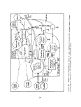 Figure 47. Model of a sub-estuary ecosystem of the Chesapeake Bay, major
components and interactions
262
image:
Figure 47. Model of a sub-estuary ecosystem of the Chesapeake Bay, major
components and interactions
262
image:
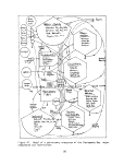 Benthic macrophytes (SAV) also take up nutrients and absorb sunlight for
photosynthesis. However, in competition with phytoplankton SAV have the distinct
disadvantage of growing from the bottom up (and thus having less access to
light than phytoplankton which can be suspended near the water surface), but
SAV have the potential advantage of having been able to take nutrients from
the sediment waters, as well as from the water column. (McRoy and Barsdate 1970;
McRoy et al. 1972; Best and Nantai 1977). Epifaunal animals living on the
macrophyte structure, feed on epiphytes and detritus on the SAV leaves, keeping
them clean and partly free of materials which block light from the leaves
(Nagle 1968). Both SAV and phytoplankton death contribute to the organic
deposits in the sediments. At high concentrations, various herbicides in the
water column and sediments may inhibit photosynthesis of phytoplankton and SAV.
However, phytoplankton have the potential advantage of being continuously
seeded from external sources and having fast growth rates, so that if herbicides
enter the system in pulses (Wu 1977) then phytoplankton can rejuvenate after
a general mortality more quickly than SAV.
Zooplankton are similarly being continuously seeded from external sources.
They filter phytoplankton and detritus from the water column and excrete
nutrients which can then be recycled. Zooplankton consist of several different
types distinguished by size, taxa, trophic habits or life cycle; and include
both meroplankton and holoplankton, copepods and large neomysis, and carnivorous
ctenophores and chaetognaths. Benthic invertegrates feed on detritus and
phytoplankton filtered from the water column and on detritus deposited in the
sediments. Their excretion and physical disruptive activities also keep
nutrients cycling back to water column storages. These benthic infauna
include filter-feeding types such as oysters, clams, barnacles, hydroids,
and other polyps; deposit-feeders such as snails and worms; some herbivorous
urchins and snails; and a few carnivorous crabs, drills and polychaetes.
Nekton are grouped in this model according to main habitat type. The pelagic
nekton include mostly planktivorous fish and their predators (bluefish).
Demersal nekton include the forage fish which feed on benthic infauna and
epifauna, as well as detrital matter, and their predators (striped bass). Both
groups of fish migrate in and out of the ecosystem according to some seasonal
cues (temperature, photoperiod, and etc.).
In Figure 48 the detailed mechanistic relationships between model components
are explicitly shown. In this version of the sub-estuary model the level of
aggregation is defined according to those variables considered most important
to the overall ecosystem dynamics and to the basic issues addressed: 1) why
have SAV declined, and 2) what is the effect of this decline on the dynamics
of economically important populations? Some of the important features of this
model not previously discussed in the more general version (Figure 47) are
discussed below.
Temperature is an important interactive, external variable, involved in five
metabolic functions in the system, and controlling five logic switches. Almost
all of the heterotrophic components of the model are shown to have respiration
and/or mortality as a function of density (i.e., state-variable interacting
with itself in an outflow through a boxed-arrow). A large die-off of SAV
through a switching function is designed to occur at the end of the growing
season when temperatures go below a threshold. The deposited detritus is shown
263
image:
Benthic macrophytes (SAV) also take up nutrients and absorb sunlight for
photosynthesis. However, in competition with phytoplankton SAV have the distinct
disadvantage of growing from the bottom up (and thus having less access to
light than phytoplankton which can be suspended near the water surface), but
SAV have the potential advantage of having been able to take nutrients from
the sediment waters, as well as from the water column. (McRoy and Barsdate 1970;
McRoy et al. 1972; Best and Nantai 1977). Epifaunal animals living on the
macrophyte structure, feed on epiphytes and detritus on the SAV leaves, keeping
them clean and partly free of materials which block light from the leaves
(Nagle 1968). Both SAV and phytoplankton death contribute to the organic
deposits in the sediments. At high concentrations, various herbicides in the
water column and sediments may inhibit photosynthesis of phytoplankton and SAV.
However, phytoplankton have the potential advantage of being continuously
seeded from external sources and having fast growth rates, so that if herbicides
enter the system in pulses (Wu 1977) then phytoplankton can rejuvenate after
a general mortality more quickly than SAV.
Zooplankton are similarly being continuously seeded from external sources.
They filter phytoplankton and detritus from the water column and excrete
nutrients which can then be recycled. Zooplankton consist of several different
types distinguished by size, taxa, trophic habits or life cycle; and include
both meroplankton and holoplankton, copepods and large neomysis, and carnivorous
ctenophores and chaetognaths. Benthic invertegrates feed on detritus and
phytoplankton filtered from the water column and on detritus deposited in the
sediments. Their excretion and physical disruptive activities also keep
nutrients cycling back to water column storages. These benthic infauna
include filter-feeding types such as oysters, clams, barnacles, hydroids,
and other polyps; deposit-feeders such as snails and worms; some herbivorous
urchins and snails; and a few carnivorous crabs, drills and polychaetes.
Nekton are grouped in this model according to main habitat type. The pelagic
nekton include mostly planktivorous fish and their predators (bluefish).
Demersal nekton include the forage fish which feed on benthic infauna and
epifauna, as well as detrital matter, and their predators (striped bass). Both
groups of fish migrate in and out of the ecosystem according to some seasonal
cues (temperature, photoperiod, and etc.).
In Figure 48 the detailed mechanistic relationships between model components
are explicitly shown. In this version of the sub-estuary model the level of
aggregation is defined according to those variables considered most important
to the overall ecosystem dynamics and to the basic issues addressed: 1) why
have SAV declined, and 2) what is the effect of this decline on the dynamics
of economically important populations? Some of the important features of this
model not previously discussed in the more general version (Figure 47) are
discussed below.
Temperature is an important interactive, external variable, involved in five
metabolic functions in the system, and controlling five logic switches. Almost
all of the heterotrophic components of the model are shown to have respiration
and/or mortality as a function of density (i.e., state-variable interacting
with itself in an outflow through a boxed-arrow). A large die-off of SAV
through a switching function is designed to occur at the end of the growing
season when temperatures go below a threshold. The deposited detritus is shown
263
image:
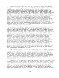 Figure 48. Model of a sub-estuary ecosystem of the Chesapeake Bay, mech-
anistic details appropriate for mathematical translation and eventual
computer simulation
264
image:
Figure 48. Model of a sub-estuary ecosystem of the Chesapeake Bay, mech-
anistic details appropriate for mathematical translation and eventual
computer simulation
264
image:
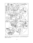 in two parts, separated by particle size, because of differences in time-con-
stants and because the smaller pieces are known to be more nutritious (with
more microbes per particle mass) (Odum 1970). A detail to the demersal nekton
population structure is indicated with two separate life-stages considered.
This was done because the juveniles of species such as white perch and striped
bass are reported to depend on SAV for habitat (i.e. a refuge from predation)
and for food, epifauna (e.g., Hollis 1952; Adams 1976a,b). SAV may thus affect
recruitment success and overall population vitality.
A highly simplified model of a Chesapeake Bay sub-estuary is shown in
Figure 49. This model was designed and simulated by W. Boynton and F. Lipschultz
to investigate productivity and nutrient dynamics of the Bay, and we include it
in this report merely as an example of some kinds of output that can be ex-
pected from ecosystem models such as that shown in Figure 47. The model was
developed to examine the major influences on nutrient recycling in the upper
Chesapeake bay. The model was found useful in providing insight into effects
of summer stratification and fall turnover on ecosystem dynamics in the euphotoic
zone. The effects of Susquehanna River flow on nutrient levels was also in-
vestigated with this model.
MATHEMATICAL EQUATIONS FOR MODEL SIMULATION
The time-varying behavior of an ecosystem model can be studied by transform-
ing the initial conceptualization into mathematical terms. Each model state-
variable has a differential equation to describe its dynamic character. Each
input and output pathway to aid from the state-variable represents a single term
in the equation for that variable, and each pathway represents some process
which affects the variable. The terms in each equation may be linear (con-
taining only one variable) or nonlinear (being a function of several variable
and/or a power, exponential, logarithmic, etc. function of one variable).
The differential equations are written with the change in quantity of each
variable per unit change in time (or space) equal to the sum of all input and
output terms. Since each term is a function of model variables themselves,
which are changing with time, the entire model system exhibits a dynamic be-
havior.
Notice in Figure 48 that the model contains 15 state-variables, and thus
needs 15 differential equations to be described. Similarly, in Figure 5jD we see
that there are five variables which need five equations for mathematical
description. The equations used for these models are given in Tables 84, 85 and
86,respectively, with a general word description for each term. Terms in
each equation which are controlled (on and off) by some external logic function
(such as temperature and photoperiod thresholds to start fish migration) are
indicated with a bracket above them. A dot above the symbol for a state-
variable indicates the instantaneous-rate-of change for that variable, or in
differential notation, dQ/dt. Pathway coefficients, indicated as k-j,j, re-
present the inherent characteristics in a pathway which are invariant within
the time-and space-frame of the model. The "i" represents the donor or source
of the flow (e.g. state-variable,(Q^) and the "j" represents the recipient of
the flow (Qj). In general, subscripting provides a description of variables
and pathways, while superscripting indicates power functions.
265
image:
in two parts, separated by particle size, because of differences in time-con-
stants and because the smaller pieces are known to be more nutritious (with
more microbes per particle mass) (Odum 1970). A detail to the demersal nekton
population structure is indicated with two separate life-stages considered.
This was done because the juveniles of species such as white perch and striped
bass are reported to depend on SAV for habitat (i.e. a refuge from predation)
and for food, epifauna (e.g., Hollis 1952; Adams 1976a,b). SAV may thus affect
recruitment success and overall population vitality.
A highly simplified model of a Chesapeake Bay sub-estuary is shown in
Figure 49. This model was designed and simulated by W. Boynton and F. Lipschultz
to investigate productivity and nutrient dynamics of the Bay, and we include it
in this report merely as an example of some kinds of output that can be ex-
pected from ecosystem models such as that shown in Figure 47. The model was
developed to examine the major influences on nutrient recycling in the upper
Chesapeake bay. The model was found useful in providing insight into effects
of summer stratification and fall turnover on ecosystem dynamics in the euphotoic
zone. The effects of Susquehanna River flow on nutrient levels was also in-
vestigated with this model.
MATHEMATICAL EQUATIONS FOR MODEL SIMULATION
The time-varying behavior of an ecosystem model can be studied by transform-
ing the initial conceptualization into mathematical terms. Each model state-
variable has a differential equation to describe its dynamic character. Each
input and output pathway to aid from the state-variable represents a single term
in the equation for that variable, and each pathway represents some process
which affects the variable. The terms in each equation may be linear (con-
taining only one variable) or nonlinear (being a function of several variable
and/or a power, exponential, logarithmic, etc. function of one variable).
The differential equations are written with the change in quantity of each
variable per unit change in time (or space) equal to the sum of all input and
output terms. Since each term is a function of model variables themselves,
which are changing with time, the entire model system exhibits a dynamic be-
havior.
Notice in Figure 48 that the model contains 15 state-variables, and thus
needs 15 differential equations to be described. Similarly, in Figure 5jD we see
that there are five variables which need five equations for mathematical
description. The equations used for these models are given in Tables 84, 85 and
86,respectively, with a general word description for each term. Terms in
each equation which are controlled (on and off) by some external logic function
(such as temperature and photoperiod thresholds to start fish migration) are
indicated with a bracket above them. A dot above the symbol for a state-
variable indicates the instantaneous-rate-of change for that variable, or in
differential notation, dQ/dt. Pathway coefficients, indicated as k-j,j, re-
present the inherent characteristics in a pathway which are invariant within
the time-and space-frame of the model. The "i" represents the donor or source
of the flow (e.g. state-variable,(Q^) and the "j" represents the recipient of
the flow (Qj). In general, subscripting provides a description of variables
and pathways, while superscripting indicates power functions.
265
image:
 <d
c
d.
s-
(U
c
01
in
<u
-o
CQ
O>
0)
Q,
(O
to
Ol
(O
3
(U 10
I U
.a -r-
(0 +J
i— C
(U d)
Q.T-
(1) -r-
•r- >
M- -I-
•t- +->
i— O
Q. 3
E TD
•r- O
oo s-
a_
. M-
CT> O
O) d)
S- •!-
3 T3
CT> 3
•r- -(->
U- to
266
image:
<d
c
d.
s-
(U
c
01
in
<u
-o
CQ
O>
0)
Q,
(O
to
Ol
(O
3
(U 10
I U
.a -r-
(0 +J
i— C
(U d)
Q.T-
(1) -r-
•r- >
M- -I-
•t- +->
i— O
Q. 3
E TD
•r- O
oo s-
a_
. M-
CT> O
O) d)
S- •!-
3 T3
CT> 3
•r- -(->
U- to
266
image:
 CO
<u
J*
to
<u
CL
s_
<u
a.
CL
<u
0)
•a
IT)
(U
<d
to
(/) (/I
(O 0)
0.
OJ
-(->
i— O
•i- £
U. Q.
CM
o
-O
<u $-
-P <a
ns o
* O
•i- £ O>
o
i- c e
4J <O *-^
s- cn<_>
<a s-
D. O CT
</>
en
coo
O -r- i—
O OQ X
O
03
i— </)
O. </XM
O « E
+J E ^x
>> O O
JC 'r-
Q. CD Cn
00
o
u
0)
i-
O
4J
2
Q.
4->
3
O
0)
CL
to
o
in
267
image:
CO
<u
J*
to
<u
CL
s_
<u
a.
CL
<u
0)
•a
IT)
(U
<d
to
(/) (/I
(O 0)
0.
OJ
-(->
i— O
•i- £
U. Q.
CM
o
-O
<u $-
-P <a
ns o
* O
•i- £ O>
o
i- c e
4J <O *-^
s- cn<_>
<a s-
D. O CT
</>
en
coo
O -r- i—
O OQ X
O
03
i— </)
O. </XM
O « E
+J E ^x
>> O O
JC 'r-
Q. CD Cn
00
o
u
0)
i-
O
4J
2
Q.
4->
3
O
0)
CL
to
o
in
267
image:
 Table 84 . Differential equations for model shown in Figure 48.
1) Nitrogen in Water Column:
Q = J - k QF-k (J )
1 1,0 1 1,5 5,5
import export phytoplanktonic uptake
- k (0 ) + k Q
1,7 7,7' 15,1 15
macrophytic uptake nitrogen fixation
+ k(J +0 +J +J )
1 6,6 15,15 3,3 12,12
excretion and recycling
+ k (Q - Q ) Q D
1,88 1 12
sediment/water exchange
2) Herbicide in Water Column:
Q = J -kQF-k (J)
2 2 2,02 2,5 5,5
import export phytoplanktonic uptake
- k D (Q - Q ) - k Q
2,9 9 2 2,22
sediment/water exchange decay
- k (J )
27 77
> >
macrophytic uptake
3) Seston in Water Column:
Q = J -kQF -J
3 3 303 36
import export zooplantkon grazing
- k Q Q - k Q Q eai2T - k Q
3,4 X3 4 3,12X3 ^12 3loX
nektonic uptake benthic uptake sedimentation
3 3 Q3
'
+ k (Q + Q ) + k Q - k3 3 Q3 ea3T
10,310 11 5,35
resuspension phytoplankton death respiration
268
image:
Table 84 . Differential equations for model shown in Figure 48.
1) Nitrogen in Water Column:
Q = J - k QF-k (J )
1 1,0 1 1,5 5,5
import export phytoplanktonic uptake
- k (0 ) + k Q
1,7 7,7' 15,1 15
macrophytic uptake nitrogen fixation
+ k(J +0 +J +J )
1 6,6 15,15 3,3 12,12
excretion and recycling
+ k (Q - Q ) Q D
1,88 1 12
sediment/water exchange
2) Herbicide in Water Column:
Q = J -kQF-k (J)
2 2 2,02 2,5 5,5
import export phytoplanktonic uptake
- k D (Q - Q ) - k Q
2,9 9 2 2,22
sediment/water exchange decay
- k (J )
27 77
> >
macrophytic uptake
3) Seston in Water Column:
Q = J -kQF -J
3 3 303 36
import export zooplantkon grazing
- k Q Q - k Q Q eai2T - k Q
3,4 X3 4 3,12X3 ^12 3loX
nektonic uptake benthic uptake sedimentation
3 3 Q3
'
+ k (Q + Q ) + k Q - k3 3 Q3 ea3T
10,310 11 5,35
resuspension phytoplankton death respiration
268
image:
 4) Pelagic Nekton;
Q = |J - J I + k Q Q
4 0,4 4 5 0 35't,3 "*
seasonal migration feeding on seston
+ kQQ +kQQ
6,464 5,454
feeding on zoopl. feeding on nekton
- k (Q )2 + J
4,44 14 ,4
respiration feeding on juveniles
5) Phytoplankton:
o
Q = J -kQF - k Q
5 5 5,05 5,35
import export death
- J + J
5, 6 5, 5
zooplankton grazing primary productivity
- k Q easT - k Q Q
5 ,16 5 5,454
respiration nektonic grazing
- k Q Q eai2T
5,12 5 X12
benthic grazing
6) Zooplankton:
o
Qfi=Jc -k QF -kQQ
y6 6 6 ,0 ^6 6 54 4 b
import export nektonic predation
+ k (J + J ) - k (Q Y
6 »6 3 s<> 5 ,6 6 ,6 6
grazing on phytopl. and seston respiration
269
image:
4) Pelagic Nekton;
Q = |J - J I + k Q Q
4 0,4 4 5 0 35't,3 "*
seasonal migration feeding on seston
+ kQQ +kQQ
6,464 5,454
feeding on zoopl. feeding on nekton
- k (Q )2 + J
4,44 14 ,4
respiration feeding on juveniles
5) Phytoplankton:
o
Q = J -kQF - k Q
5 5 5,05 5,35
import export death
- J + J
5, 6 5, 5
zooplankton grazing primary productivity
- k Q easT - k Q Q
5 ,16 5 5,454
respiration nektonic grazing
- k Q Q eai2T
5,12 5 X12
benthic grazing
6) Zooplankton:
o
Qfi=Jc -k QF -kQQ
y6 6 6 ,0 ^6 6 54 4 b
import export nektonic predation
+ k (J + J ) - k (Q Y
6 »6 3 s<> 5 ,6 6 ,6 6
grazing on phytopl. and seston respiration
269
image:
 7) Benthic Macrophytes (SAV):
Q = J
V7 7,7
primary productivity
winter die off
- k Q e
7,16 7
,a7T
respiration
15
herbivory
continual death
8) Nitrogen in Sediments:
4, ' k1>8 (Q. - Q, ) Q12 D
sediment/water exchange
+ k (0 \ pai°T
T "MI,eVvii/ e
tnacro-detritus respiration
9) Herbicide in Sediments:
|o
Q<
= k D (Q - Q )
2,9 9 2
sediment/water exchange
micro-detri. respir.
- k (J )
8,7 7,7'
macrophytic uptake
- k Q
9 ,9 9
decay
10) Ifticro-Detritus in Sediments:
= k (J )
10 12,10 11,12
break-down of macro-detritus by benthics
10, 12
benthic grazing
- k
aioT
10,10
10
respiration
break-down of macro-detritus by nekton
270
image:
7) Benthic Macrophytes (SAV):
Q = J
V7 7,7
primary productivity
winter die off
- k Q e
7,16 7
,a7T
respiration
15
herbivory
continual death
8) Nitrogen in Sediments:
4, ' k1>8 (Q. - Q, ) Q12 D
sediment/water exchange
+ k (0 \ pai°T
T "MI,eVvii/ e
tnacro-detritus respiration
9) Herbicide in Sediments:
|o
Q<
= k D (Q - Q )
2,9 9 2
sediment/water exchange
micro-detri. respir.
- k (J )
8,7 7,7'
macrophytic uptake
- k Q
9 ,9 9
decay
10) Ifticro-Detritus in Sediments:
= k (J )
10 12,10 11,12
break-down of macro-detritus by benthics
10, 12
benthic grazing
- k
aioT
10,10
10
respiration
break-down of macro-detritus by nekton
270
image:
 1 1 ) Macro-Detritus in Sediments:
Q = 7k qT
11
7,11
winter macrophytic die-off
+ k Q
17,11 7
continual macrophytic death
- k
11,11
respiration
Q ec
11
- J
11,12
benthic grazing
- k Q Q
11,13 11 13
nekton grazing
12) Benthic invertebrates:
Q = (J
X 12 3,12
12
suspension-feeding
- k
Q Q
12 13
nektonic predation
12,13
iO,12 11,1
deposit - feeding
- k
(Q )
12,12 12
respiration
13) Demersal Nekton. Adults:
= id
0 3
3,0
seasonal migration
+ k Q Q
11,13 11 13
feeding on detritus
+ k Q Q
12,13 12 13
feeding on benthics
+ k Q '
14 ,1 3 l«t
recruitment
-'k
13,1"* 13
spawning
- k
1 3 91 3
respiration
(Q )
1 3
14) Demersal Nekton, Juveniles:
Q = k Q Q
i1* is, m m is
feeding on epifauna
- J
predation by nekton
- k^^ (Q^)2
respiration
-'k
1 3, If
spawning
13
14,13 Ik
recruitment
271
image:
1 1 ) Macro-Detritus in Sediments:
Q = 7k qT
11
7,11
winter macrophytic die-off
+ k Q
17,11 7
continual macrophytic death
- k
11,11
respiration
Q ec
11
- J
11,12
benthic grazing
- k Q Q
11,13 11 13
nekton grazing
12) Benthic invertebrates:
Q = (J
X 12 3,12
12
suspension-feeding
- k
Q Q
12 13
nektonic predation
12,13
iO,12 11,1
deposit - feeding
- k
(Q )
12,12 12
respiration
13) Demersal Nekton. Adults:
= id
0 3
3,0
seasonal migration
+ k Q Q
11,13 11 13
feeding on detritus
+ k Q Q
12,13 12 13
feeding on benthics
+ k Q '
14 ,1 3 l«t
recruitment
-'k
13,1"* 13
spawning
- k
1 3 91 3
respiration
(Q )
1 3
14) Demersal Nekton, Juveniles:
Q = k Q Q
i1* is, m m is
feeding on epifauna
- J
predation by nekton
- k^^ (Q^)2
respiration
-'k
1 3, If
spawning
13
14,13 Ik
recruitment
271
image:
 15) Epifauna! Coirynunity:
o
grazing epiphytes ^°e4atfen by nekton
- k,s.s («,. >2 '°"5T
272
image:
15) Epifauna! Coirynunity:
o
grazing epiphytes ^°e4atfen by nekton
- k,s.s («,. >2 '°"5T
272
image:
 Table 85, Special functions used in equations given in Tab'tc &4.
1 ) Primary Productivity, Phytoplankton;
(ea*,5 ) ( I + aQJ (1 + b5L) (1 - C5es 12)
temperature nitrogen sunlight herbicide inhibition
2) Primary Productivity. Macrophytes:
, (Qi + 0.8 ')
j ) ( 1 + b7L) Q7 (1 + d7 Q15)
temperature nitrogen sunlight epifaunal cleaning
herbicide inhibition
3) Shading of Sunlight:
L = L (K - ea<>(Q3+ QS))
4 ) Zooplankton Grazing on Seston:
5) Zooplankton Grazing on Phytoplankton:
Js,e = ks,6(ea3T ) Qe QS
6) Benthic Invertebrates Feeding, on Phytoplankton
population
management
7) Benthic Invertebrates Feeding, on others:
12
where i is food item:
Macro-Detritus, i = 11
Micro- Detritus, i = 10
Seston, i = 3
273
image:
Table 85, Special functions used in equations given in Tab'tc &4.
1 ) Primary Productivity, Phytoplankton;
(ea*,5 ) ( I + aQJ (1 + b5L) (1 - C5es 12)
temperature nitrogen sunlight herbicide inhibition
2) Primary Productivity. Macrophytes:
, (Qi + 0.8 ')
j ) ( 1 + b7L) Q7 (1 + d7 Q15)
temperature nitrogen sunlight epifaunal cleaning
herbicide inhibition
3) Shading of Sunlight:
L = L (K - ea<>(Q3+ QS))
4 ) Zooplankton Grazing on Seston:
5) Zooplankton Grazing on Phytoplankton:
Js,e = ks,6(ea3T ) Qe QS
6) Benthic Invertebrates Feeding, on Phytoplankton
population
management
7) Benthic Invertebrates Feeding, on others:
12
where i is food item:
Macro-Detritus, i = 11
Micro- Detritus, i = 10
Seston, i = 3
273
image:
 Table 86. Differential equations for model shown in Figure 49
1) Phytoplankton;
4)
producitivity death predation
klj6 Qt - 0.24 Qx + 0.0006
export respiration import
2) Consumers:
.75T
feeding on phytopl.
- 0.25 Q2
export and death
3) Detritus:
feeding on detritus
+ 0.0009
import
o
Q3 -J
river
- k
3,7
0,3
input
Q
3
+ 0.125 Qj + k
phytopl .
death
- k Q
3,6 3
•3(kl,2Ql + K3,A } Q
consumer excretion
- k Q Q e'
3,2 2 3
e
2
75T
. 75T
sedimentation
Phosphate:
o
Qiit = Jfl ^
river input
detritus
regeneration
export
+ J H
sediment
regeneration
- k Q Q Q L
*»,! 1 "t 5
phytoplankton
uptake
consumer grazing
(.125)0
i
phytopl. excretion
- k A
4,6 K
export
274
image:
Table 86. Differential equations for model shown in Figure 49
1) Phytoplankton;
4)
producitivity death predation
klj6 Qt - 0.24 Qx + 0.0006
export respiration import
2) Consumers:
.75T
feeding on phytopl.
- 0.25 Q2
export and death
3) Detritus:
feeding on detritus
+ 0.0009
import
o
Q3 -J
river
- k
3,7
0,3
input
Q
3
+ 0.125 Qj + k
phytopl .
death
- k Q
3,6 3
•3(kl,2Ql + K3,A } Q
consumer excretion
- k Q Q e'
3,2 2 3
e
2
75T
. 75T
sedimentation
Phosphate:
o
Qiit = Jfl ^
river input
detritus
regeneration
export
+ J H
sediment
regeneration
- k Q Q Q L
*»,! 1 "t 5
phytoplankton
uptake
consumer grazing
(.125)0
i
phytopl. excretion
- k A
4,6 K
export
274
image:
 5) Nitrogen:
Q=J +kQ + k (.125Q )
5 0,5 3,53 1,5 1
river detritus phytopl. excretion
input regeneration
4- k (k Q Q e<75r + k Q Q e'1®
2,52,112 2,323
consumer excretion of ammonia
+ J -kQ -kQQQL
8,5 5,6 5 5,1 1 i* 5
sediment export phytopl. uptake
regeneration
275
image:
5) Nitrogen:
Q=J +kQ + k (.125Q )
5 0,5 3,53 1,5 1
river detritus phytopl. excretion
input regeneration
4- k (k Q Q e<75r + k Q Q e'1®
2,52,112 2,323
consumer excretion of ammonia
+ J -kQ -kQQQL
8,5 5,6 5 5,1 1 i* 5
sediment export phytopl. uptake
regeneration
275
image:
 CALIBRATION OF MODEL
To make the model operational, pathway coefficients involved in each term
of each equation must be numerically evaluated or calibrated. Each equation
term represents a flow of material, energy, or information which is stated as
a function of one or more model state-variables and one (occasionally more)
coefficient that characterizes inherent properties of the pathway. The model is
calibrated by estimating the values of these coefficients. If data are available
for a small time segment to establish the actual flow, as indicated by a given
equation term, and the mean levels of each state-variable involved in that
term, then the coefficient for the term can be algebraically calculated.
Numerical values must also be assigned for the model's external forcing functions.
Here, such factors as sunlight and temperature, which are external to the
boundaries defined for the model in Figure 49are described either by discontinuous
time-series of input data or by some continuous function fit to that data.
With model coefficients and forcing functions numerically defined, and with
initial values (starting points) assigned to each state-variable, the model is
ready to be programmed and simulated on a computer.
If we were to try to calibrate and simulate the model given in Figure 48
and Tables 84 and 85 for a particular sub-basin of the Bay, we would first
seek all available information describing the structural and functional parts
of that sub-Bay contained in the model. For the Patuxent estuarine ecosystem
considerable amount of such data is available, and is summarized in Table 87.
Comparing the variables listed in this table against the variables given in
the model equations of Table 84 (where each Q is a state-variable and each
equation term is a flow variable), we find that the available data fills about
15 percent of the data needed to calibrate this model. This disparity between
needs and availability helps to demonstrate major lacunae in the general state
of our knowledge about this system. In Table 88 several additional pieces
of data pertinent to the model are provided mostly from other similar ecosystems.
The number of data values needed to completely calibrate this model can be
reduced by the number of equations (15 in this case) by carefully selecting
the time for calibration from the time-series of data, and by making a simple
assumption of steady-state. If we calibrate the model from mid-winter data,
for instance, we can assume that most ecological state-variables are at or near
a minimum value. Thus, their rate-of-change is close to zero. By assuming
that these rates-of-change are equal to zero, we can estimate one term in the
equation if we know all the others. An example will illustrate the process of
calculating coefficients. In equation 6 of Table 84 we find that zooplankton
respiration is represented by k6,6(Q6)2. In August zooplankton biomass was
.025gC/m2 and respiration was .005 gC/m2d, and we thus calculate the respiration
coefficient k6>6= (.005)/(.025)2= 8.Q. (Table 79).
SIMULATION OF MODEL
Once the model is fully calibrated it can be numerically simulated on an
analog or digital computer. Initial simulation runs involve fine-tuning adjust-
ments of coefficients to match model behavior with field data. In some cases,
where no amount of coefficient adjustment can improve the fit of model to data,
276
image:
CALIBRATION OF MODEL
To make the model operational, pathway coefficients involved in each term
of each equation must be numerically evaluated or calibrated. Each equation
term represents a flow of material, energy, or information which is stated as
a function of one or more model state-variables and one (occasionally more)
coefficient that characterizes inherent properties of the pathway. The model is
calibrated by estimating the values of these coefficients. If data are available
for a small time segment to establish the actual flow, as indicated by a given
equation term, and the mean levels of each state-variable involved in that
term, then the coefficient for the term can be algebraically calculated.
Numerical values must also be assigned for the model's external forcing functions.
Here, such factors as sunlight and temperature, which are external to the
boundaries defined for the model in Figure 49are described either by discontinuous
time-series of input data or by some continuous function fit to that data.
With model coefficients and forcing functions numerically defined, and with
initial values (starting points) assigned to each state-variable, the model is
ready to be programmed and simulated on a computer.
If we were to try to calibrate and simulate the model given in Figure 48
and Tables 84 and 85 for a particular sub-basin of the Bay, we would first
seek all available information describing the structural and functional parts
of that sub-Bay contained in the model. For the Patuxent estuarine ecosystem
considerable amount of such data is available, and is summarized in Table 87.
Comparing the variables listed in this table against the variables given in
the model equations of Table 84 (where each Q is a state-variable and each
equation term is a flow variable), we find that the available data fills about
15 percent of the data needed to calibrate this model. This disparity between
needs and availability helps to demonstrate major lacunae in the general state
of our knowledge about this system. In Table 88 several additional pieces
of data pertinent to the model are provided mostly from other similar ecosystems.
The number of data values needed to completely calibrate this model can be
reduced by the number of equations (15 in this case) by carefully selecting
the time for calibration from the time-series of data, and by making a simple
assumption of steady-state. If we calibrate the model from mid-winter data,
for instance, we can assume that most ecological state-variables are at or near
a minimum value. Thus, their rate-of-change is close to zero. By assuming
that these rates-of-change are equal to zero, we can estimate one term in the
equation if we know all the others. An example will illustrate the process of
calculating coefficients. In equation 6 of Table 84 we find that zooplankton
respiration is represented by k6,6(Q6)2. In August zooplankton biomass was
.025gC/m2 and respiration was .005 gC/m2d, and we thus calculate the respiration
coefficient k6>6= (.005)/(.025)2= 8.Q. (Table 79).
SIMULATION OF MODEL
Once the model is fully calibrated it can be numerically simulated on an
analog or digital computer. Initial simulation runs involve fine-tuning adjust-
ments of coefficients to match model behavior with field data. In some cases,
where no amount of coefficient adjustment can improve the fit of model to data,
276
image:
 Table 87. Some data from related ecosystems useful in calibrating a model of
Patuxent estuarine ecosystem
Variable
Mean
Value
Ecosystem
Reference
Rate of Sediment Deposition
Carbon Content of Sediment
Carbon/Nitrogen of Sediment
Epifaunal Biomass
Epifaunal Assimilation
Epifaunal Respiration
Benthic Invertebrate Biomass
Benthic Assimilation
Benthic Respiration
Sediment Detrital Respir.
Demersal Fish Biomass
Demersal Fish Respiration
Demersal Fish Consumption
Macrophyte Biomass
14 mm/yr
1.8%
14
.47gC/m2
.018gC/m2/d
.014gC/m2/d
3.31gC/m2
.06gC/m2/d
.05gC/m2/d
.62gC/m2/d
.78gC/m2
.02gC/m2/d
.03gC/m2/d
230gC/m2
53gC/m2
Coastal Eel grass
Coastal Eel grass
Patuxent Estuary
Coastal Eel grass
Coastal Eelgrass
Coastal Eelgrass
Coastal Eelgrass
Coastal Eelgrass
Coastal Eelgrass
Georgia Estuary
Coastal Eelgrass
Coastal Eelgrass
Coastal Eelgrass
Eelgrass
Eelgrass
Thayer et al, (1975)
Thayer et al. (1975)
Flemer et al. (1970)
Thayer et al. (1975)
Thayer et al. (1975)
Thayer et al. (1975)
Thayer et al. (1975)
Thayer et al. (1975)
Thayer et al.(1975)
Smith (1971)
Adams (1976a,b)
Adams (1976a,b)
Adams (1976a,b)
McRoy (1970a)
Penhale (1977)
277
image:
Table 87. Some data from related ecosystems useful in calibrating a model of
Patuxent estuarine ecosystem
Variable
Mean
Value
Ecosystem
Reference
Rate of Sediment Deposition
Carbon Content of Sediment
Carbon/Nitrogen of Sediment
Epifaunal Biomass
Epifaunal Assimilation
Epifaunal Respiration
Benthic Invertebrate Biomass
Benthic Assimilation
Benthic Respiration
Sediment Detrital Respir.
Demersal Fish Biomass
Demersal Fish Respiration
Demersal Fish Consumption
Macrophyte Biomass
14 mm/yr
1.8%
14
.47gC/m2
.018gC/m2/d
.014gC/m2/d
3.31gC/m2
.06gC/m2/d
.05gC/m2/d
.62gC/m2/d
.78gC/m2
.02gC/m2/d
.03gC/m2/d
230gC/m2
53gC/m2
Coastal Eel grass
Coastal Eel grass
Patuxent Estuary
Coastal Eel grass
Coastal Eelgrass
Coastal Eelgrass
Coastal Eelgrass
Coastal Eelgrass
Coastal Eelgrass
Georgia Estuary
Coastal Eelgrass
Coastal Eelgrass
Coastal Eelgrass
Eelgrass
Eelgrass
Thayer et al, (1975)
Thayer et al. (1975)
Flemer et al. (1970)
Thayer et al. (1975)
Thayer et al. (1975)
Thayer et al. (1975)
Thayer et al. (1975)
Thayer et al. (1975)
Thayer et al.(1975)
Smith (1971)
Adams (1976a,b)
Adams (1976a,b)
Adams (1976a,b)
McRoy (1970a)
Penhale (1977)
277
image:
 E
<D Q
+J
CO
>}
CO
O z
o
0)
(U
*•
•^~
i- 0
(O
CO
fll
C-O
+j
G
O)
X
«J
*^"^ ^C
ro
D.
<*-
^3
r-^
F™*
O)
TD
£ s-
18 I °
C 0
•r-
+J 5 x:
(O c
S- 0
-d z:
*F"
to
<c
S-
0
r— x:
(0
F"""
(O ^
^^ ^^
"3 fO
CO
•p tt)
•o «j
i— <O
-C CO *j
C^~
•^" ™"1
§0
«f-^
O 4J
^^Ci—
^* /•%
(0
C ?">
3 (0
1/1 5
* _ (y
00 jQ •«
00 3 •£
0) >
[Q
ra en
0 C3
T^ CM
in in
oo *a-
in
••H CM
in
f^ CO
CM
in
en •
CM to
in
00
CM ^f
o
10
CM CO
in
0
CO
CM CO
o
o
•-H CO
in in
CO CO
O en
CM CM
in o
CO CM
o
O 1
1>
c
01
•r—
U
|JI
M-
O)
« S
O>
S- C
3 •?
<C -P
i- U
V ,C
S X
h- LU
1
CO
C3
in
T-H
0
««•
to
•
^
00
^-
CO
in
o
•
CO
in
CM
CO
o
o
I-H
1
•o
"*^
"e
{j
O)
^3
^o
8
a'
V)
I/I
2
o
>>
•r-
C
3
g
O
CM
in
1 1 1 1 1 1 O
in
O CM
0 .-H 0 tj-
o oo o o o o in
o
CM O i-H 00
in
o in
O t-H i— * *3-
OCnCMOOOCOO
....... o
CO O i-H i-H
CM in
in o CM I-H vo
o en co o o o I-H
o
CM »-1 «i-
i-H i-l
in in
O CM CM O
C3 *"H ^-! C? CO <"i ^f {-^
CM
f*» »-H i-H i-H
vo in
O CO CM CO
oooi-^ooooo
....... (^i
ID O I-H I-H
o vo in CM
co in co o o o t-H
o
m o I-H en
in
o in co co
incooooooo
....... i— i
I-. O CM I-H
r--
en
O I-H
in in
l 1 1 1 1 • O >>
</)
i-
CO -C
OO I-» O i-
i i i i i ' *i- s:
0 -H
^
<c
CM
in r-» 01
1 1 1 1 I • O t-
•-H en 0)
5*Z O
o • en
en c t-H
1 1 1 1 1 1 • **• O
vo •»-> i.
T> T3 T3 T3 CO ^—
^. — . ^>. •»«. 3C U-
Ne "E NE NE "E ^k NE « j -
o o o o o o z "^ d)^"1*!*^
en o) O) m of oi o) o) E ^f* o^
f— en
1 1 ,_| gj
O • — •—
JQ 0 C >, C
c vi o cn s. -r-
O </)U<J-r- VOOOI
4-> E S- in o c I-H — -• — -
L. O "^" ^ E ^3 CD CO Cn C5
•r- i- CQ U1 O O O VDVOr-^
Q. a. oi-r-s-s- cncncn
in c ce OQ Q- +J r-Hi-H<-i
Ol 4-> O T-
CfOI-UCCCZ S- S- S-
Z-^OOO O O O
>> C +->+-> 4-> 0 l«- 14- 14-
•t-r— r— cccEio njioic
c 0.0.10 re ra ra c +-> 4-> +->
3 O Or— i— i — CT>O (OIOIO
E+J-»JQ.O,Q.1--U OOO
O-C-COOOCO)
OCvQ.lvlhs4M>-icO (O JD U
278
image:
E
<D Q
+J
CO
>}
CO
O z
o
0)
(U
*•
•^~
i- 0
(O
CO
fll
C-O
+j
G
O)
X
«J
*^"^ ^C
ro
D.
<*-
^3
r-^
F™*
O)
TD
£ s-
18 I °
C 0
•r-
+J 5 x:
(O c
S- 0
-d z:
*F"
to
<c
S-
0
r— x:
(0
F"""
(O ^
^^ ^^
"3 fO
CO
•p tt)
•o «j
i— <O
-C CO *j
C^~
•^" ™"1
§0
«f-^
O 4J
^^Ci—
^* /•%
(0
C ?">
3 (0
1/1 5
* _ (y
00 jQ •«
00 3 •£
0) >
[Q
ra en
0 C3
T^ CM
in in
oo *a-
in
••H CM
in
f^ CO
CM
in
en •
CM to
in
00
CM ^f
o
10
CM CO
in
0
CO
CM CO
o
o
•-H CO
in in
CO CO
O en
CM CM
in o
CO CM
o
O 1
1>
c
01
•r—
U
|JI
M-
O)
« S
O>
S- C
3 •?
<C -P
i- U
V ,C
S X
h- LU
1
CO
C3
in
T-H
0
««•
to
•
^
00
^-
CO
in
o
•
CO
in
CM
CO
o
o
I-H
1
•o
"*^
"e
{j
O)
^3
^o
8
a'
V)
I/I
2
o
>>
•r-
C
3
g
O
CM
in
1 1 1 1 1 1 O
in
O CM
0 .-H 0 tj-
o oo o o o o in
o
CM O i-H 00
in
o in
O t-H i— * *3-
OCnCMOOOCOO
....... o
CO O i-H i-H
CM in
in o CM I-H vo
o en co o o o I-H
o
CM »-1 «i-
i-H i-l
in in
O CM CM O
C3 *"H ^-! C? CO <"i ^f {-^
CM
f*» »-H i-H i-H
vo in
O CO CM CO
oooi-^ooooo
....... (^i
ID O I-H I-H
o vo in CM
co in co o o o t-H
o
m o I-H en
in
o in co co
incooooooo
....... i— i
I-. O CM I-H
r--
en
O I-H
in in
l 1 1 1 1 • O >>
</)
i-
CO -C
OO I-» O i-
i i i i i ' *i- s:
0 -H
^
<c
CM
in r-» 01
1 1 1 1 I • O t-
•-H en 0)
5*Z O
o • en
en c t-H
1 1 1 1 1 1 • **• O
vo •»-> i.
T> T3 T3 T3 CO ^—
^. — . ^>. •»«. 3C U-
Ne "E NE NE "E ^k NE « j -
o o o o o o z "^ d)^"1*!*^
en o) O) m of oi o) o) E ^f* o^
f— en
1 1 ,_| gj
O • — •—
JQ 0 C >, C
c vi o cn s. -r-
O </)U<J-r- VOOOI
4-> E S- in o c I-H — -• — -
L. O "^" ^ E ^3 CD CO Cn C5
•r- i- CQ U1 O O O VDVOr-^
Q. a. oi-r-s-s- cncncn
in c ce OQ Q- +J r-Hi-H<-i
Ol 4-> O T-
CfOI-UCCCZ S- S- S-
Z-^OOO O O O
>> C +->+-> 4-> 0 l«- 14- 14-
•t-r— r— cccEio njioic
c 0.0.10 re ra ra c +-> 4-> +->
3 O Or— i— i — CT>O (OIOIO
E+J-»JQ.O,Q.1--U OOO
O-C-COOOCO)
OCvQ.lvlhs4M>-icO (O JD U
278
image:
 the equations themselves must be modified according to alternative mechanisms
of interaction which correspond to documented facts or reasonable hypotheses.
After the model is adjusted to match the data from which it was calibrated,
its behavior should be "varified" or validated" by comparison with an independent
data set. Any modifications needed to meet criteria of "reasonable validation"
must involve changes in model equations rather than coefficients, so that
model characteristics can be made to match both data sets. During the process
of model verification, confidence is built in the general ability of the model
to have realistically. Eventually, then, the model would be used to investigate
system responses to modified external forcing functions. Thus, we might want
to forecast the response of our Chesapeake Bay ecosystem model to increased
turbidity, nutrients, and/or herbicides. We might remove SAV from the model
and observe how the ecosystem (particularly fisheries) reacts. Predictive
simulations allow the modeler to investigate ecosystem responses to a spectrum
of different conditions, and compare these responses to field observations to
test causative factors for ecosystem modifications.
The simplified ecosystem model of the upper Chesapeake Bay described in Fig-
ure 49 and Table 86 was simulated in some preliminary computer runs. Data for
phytoplankton biomass, detritus, light and temperature were taken (Table 88)
from Flemer (1970), while data for the consumer state-variable (comprised
primarily of zooplankton) was taken from Heinle (1974) and nutrient concentra-
tions and dynamics were based on the work of Whaley et al (1966). In Figure 50
we see that levels of nitrogen and phosphorus increase during the late fall
and winter as a result of microbial mineralizariom and lack of autotrophic
uptake. Decomposition of detritus which is carried by the river, further
increased nitrogen and phosphorus concentrations. These increases, along with
higher levels of insolation, permitted phytoplankton biomass to reach a peak
in April and May. Consumers show less seasonality probably due to their ability
to switch their feeding between detritus and phytoplankton according to which
is more abundant. Consumer standing stocks reach an annual maximum in July,
lagging about three months behind peak phytoplankton and zooplankton during
winter as a result of decreased sunlight and temperature, respectively.
This model is presented here merely to demonstrate some methodologies
involved in the simulation process. More detailed models (such as shown in
Figure 48 at several levels of focus are needed for addressing questions of
SAV interactions in the Chesapeake Bay.
279
image:
the equations themselves must be modified according to alternative mechanisms
of interaction which correspond to documented facts or reasonable hypotheses.
After the model is adjusted to match the data from which it was calibrated,
its behavior should be "varified" or validated" by comparison with an independent
data set. Any modifications needed to meet criteria of "reasonable validation"
must involve changes in model equations rather than coefficients, so that
model characteristics can be made to match both data sets. During the process
of model verification, confidence is built in the general ability of the model
to have realistically. Eventually, then, the model would be used to investigate
system responses to modified external forcing functions. Thus, we might want
to forecast the response of our Chesapeake Bay ecosystem model to increased
turbidity, nutrients, and/or herbicides. We might remove SAV from the model
and observe how the ecosystem (particularly fisheries) reacts. Predictive
simulations allow the modeler to investigate ecosystem responses to a spectrum
of different conditions, and compare these responses to field observations to
test causative factors for ecosystem modifications.
The simplified ecosystem model of the upper Chesapeake Bay described in Fig-
ure 49 and Table 86 was simulated in some preliminary computer runs. Data for
phytoplankton biomass, detritus, light and temperature were taken (Table 88)
from Flemer (1970), while data for the consumer state-variable (comprised
primarily of zooplankton) was taken from Heinle (1974) and nutrient concentra-
tions and dynamics were based on the work of Whaley et al (1966). In Figure 50
we see that levels of nitrogen and phosphorus increase during the late fall
and winter as a result of microbial mineralizariom and lack of autotrophic
uptake. Decomposition of detritus which is carried by the river, further
increased nitrogen and phosphorus concentrations. These increases, along with
higher levels of insolation, permitted phytoplankton biomass to reach a peak
in April and May. Consumers show less seasonality probably due to their ability
to switch their feeding between detritus and phytoplankton according to which
is more abundant. Consumer standing stocks reach an annual maximum in July,
lagging about three months behind peak phytoplankton and zooplankton during
winter as a result of decreased sunlight and temperature, respectively.
This model is presented here merely to demonstrate some methodologies
involved in the simulation process. More detailed models (such as shown in
Figure 48 at several levels of focus are needed for addressing questions of
SAV interactions in the Chesapeake Bay.
279
image:
 CHAPTER 6
POSSIBLE MANAGEMENT OPTIONS
Until further experimental and field research is completed, it is difficult
to determine what factor or combination of factors are actually responsible for
the submerged aquatic declines in the Chesapeake Bay. Therefore, any suggestions
of best management practices must be considered tentative at this time.
If the point source discharges from sewage and water treatment plants are
determined to constitute a major problem, tertiary treatment of wastewater may
help to some extent in relieving the high nutrient burden on SAV communities.
However, chlorination problems would still be present. Chlorination alternatives
that could be implemented immediately before discharging wastewater into the es-
tuary should be investigated.
One possibility is to pass the effluent from existing sewage treatment plants
under ultra-violet radiation sources to kill remaining pathogens before it is dis-
charged. This might greatly reduce the need for chlorination. Another possibil-
ity is to use land treatment as a final biological filter to eliminate pathogens
from the water before it reaches the Chesapeake Bay. Studies now under way at
St. Charles City, Maryland show that forested land can act as an effective buffer
in regard to bacteria. More extensive studies pioneered at Pennsylvania State
University have found similar results.
Such land disposal methods are limited primarily to low density areas where
land is both available and not prohibitive in cost. Around major cities such as
Washington, D. C. and Baltimore it may not be possible to have both submerged
aquatic vegetation and high chlorination and nutrient levels due to the necessity
of large sewage and water treatment plants.
Further management options deal with high turbidities due to sedimentation.
There is evidence that turbidity levels are lower in the 1970s (see Chapter 4).
This may be due to ever increased effectiveness at controlling soil erosion around
the perimeters of the Chesapeake Bay estuary. The use of no-till agriculture may
be a prime reason for the decreased turbidity that seems to be apparent in many
of the Bay's subestuaries during the 1970s. More work should be done to evaluate
the effects of true no-till agriculture in regard to erosion control. By contrast
to erosion from runoff, wind erosion in the drier years of 1976 and 1977 seems to
be more prevalent. Encouraging farmers to plant wind breaks along fields would
help alleviate this situation.
280
image:
CHAPTER 6
POSSIBLE MANAGEMENT OPTIONS
Until further experimental and field research is completed, it is difficult
to determine what factor or combination of factors are actually responsible for
the submerged aquatic declines in the Chesapeake Bay. Therefore, any suggestions
of best management practices must be considered tentative at this time.
If the point source discharges from sewage and water treatment plants are
determined to constitute a major problem, tertiary treatment of wastewater may
help to some extent in relieving the high nutrient burden on SAV communities.
However, chlorination problems would still be present. Chlorination alternatives
that could be implemented immediately before discharging wastewater into the es-
tuary should be investigated.
One possibility is to pass the effluent from existing sewage treatment plants
under ultra-violet radiation sources to kill remaining pathogens before it is dis-
charged. This might greatly reduce the need for chlorination. Another possibil-
ity is to use land treatment as a final biological filter to eliminate pathogens
from the water before it reaches the Chesapeake Bay. Studies now under way at
St. Charles City, Maryland show that forested land can act as an effective buffer
in regard to bacteria. More extensive studies pioneered at Pennsylvania State
University have found similar results.
Such land disposal methods are limited primarily to low density areas where
land is both available and not prohibitive in cost. Around major cities such as
Washington, D. C. and Baltimore it may not be possible to have both submerged
aquatic vegetation and high chlorination and nutrient levels due to the necessity
of large sewage and water treatment plants.
Further management options deal with high turbidities due to sedimentation.
There is evidence that turbidity levels are lower in the 1970s (see Chapter 4).
This may be due to ever increased effectiveness at controlling soil erosion around
the perimeters of the Chesapeake Bay estuary. The use of no-till agriculture may
be a prime reason for the decreased turbidity that seems to be apparent in many
of the Bay's subestuaries during the 1970s. More work should be done to evaluate
the effects of true no-till agriculture in regard to erosion control. By contrast
to erosion from runoff, wind erosion in the drier years of 1976 and 1977 seems to
be more prevalent. Encouraging farmers to plant wind breaks along fields would
help alleviate this situation.
280
image:
 Another problem which many areas of the Bay are experiencing is shoreline
erosion. The costs of arresting this natural process are so staggering that such
measures may be prohibitive on a large scale. Also since the Chesapeake Bay has
been experiencing shoreline erosion and subsequent sedimentation since its form-
ation in Pleistocene, these processes cannot alone account for SAV losses.
More important than natural erosion processes are large construction projects
and stream channelization efforts which are often responsible for dumping tremen-
dous loads of sediments into the Bay estuary. A Bay area example of such a
project is the "stream improvement" dredging being conducted by the U.S. Depart-
ment of Agriculture Soil Conservation Service in the Delaware portion of the
Choptank River. While appearing to be cost effective in Delaware because of an
increase in usable agricultural acreages, the downstream effects may prove to be
devastating not only to SAV but also to important commercial faunal species.
The possibility exists that significant leakage of new agro-chemicals into
streams and tributaries may be the cause of Baywide declines in SAV. If par-
ticular herbicides utilized in the Bay area prove to be a major problem, it may
be possible to substitute other available chemical compounds which are less harm-
ful to SAV. Before any substitutions are made, careful screening of the existing
compounds needs to be implemented at several levels. Submerged aquatics (includ-
ing their symbionts) should be bioassayed and Bay ecosystem responses need to be
determined before specific suggestions can be made.
Another management option might be to encourage area farmers to construct
ditches that lead to small ponds where complete biodegradation of chemicals would
occur before draining into the estuary. These small ponds would also act as sed-
iment traps. No changes in "minimum or no till" agriculture are suggested until
a thorough understanding of their benefits and environmental costs are tabulated,
using economic and ecological modeling approaches.
Another possibility is to reestablish SAV populations using planting tech-
niques. These techniques are currently being tested by the Maryland Department
of Natural Resources (Stotts, pers. com.). Thus far there seems to be consider-
able difficulty in establishing large beds. This may help support one of the
key conclusions in this study: that the decline in submerged aquatics is related
to some overall change in water quality of the Bay, rather than to some intrinsic
cyclic population phenomenon of the Bay ecosystem. Until we understand the dyna-
mics of the SAV decline and its implications on the Chesapeake Ecosystem, it may
not pay to attempt large scale replanting.
A more reasonable approach might be to incorporate existing productive beds
of submerged aquatics into an estuarine sanctuary. These could then be protected
from clam dredges and small boat propellers which have been suggested as negative-
ly impacting the submerged aquatic populations. This would also provide areas
where researchers could set up long term experiments which need to be done to
answer our management questions.
One final management option which should be considered is the control of
grazing waterfowl in selected sanctuary areas. This might be especially helpful
in the case of mute swans which have the potential of consuming large amounts of
submerged macrophytes. There is little evidence that the mute swans have been
281
image:
Another problem which many areas of the Bay are experiencing is shoreline
erosion. The costs of arresting this natural process are so staggering that such
measures may be prohibitive on a large scale. Also since the Chesapeake Bay has
been experiencing shoreline erosion and subsequent sedimentation since its form-
ation in Pleistocene, these processes cannot alone account for SAV losses.
More important than natural erosion processes are large construction projects
and stream channelization efforts which are often responsible for dumping tremen-
dous loads of sediments into the Bay estuary. A Bay area example of such a
project is the "stream improvement" dredging being conducted by the U.S. Depart-
ment of Agriculture Soil Conservation Service in the Delaware portion of the
Choptank River. While appearing to be cost effective in Delaware because of an
increase in usable agricultural acreages, the downstream effects may prove to be
devastating not only to SAV but also to important commercial faunal species.
The possibility exists that significant leakage of new agro-chemicals into
streams and tributaries may be the cause of Baywide declines in SAV. If par-
ticular herbicides utilized in the Bay area prove to be a major problem, it may
be possible to substitute other available chemical compounds which are less harm-
ful to SAV. Before any substitutions are made, careful screening of the existing
compounds needs to be implemented at several levels. Submerged aquatics (includ-
ing their symbionts) should be bioassayed and Bay ecosystem responses need to be
determined before specific suggestions can be made.
Another management option might be to encourage area farmers to construct
ditches that lead to small ponds where complete biodegradation of chemicals would
occur before draining into the estuary. These small ponds would also act as sed-
iment traps. No changes in "minimum or no till" agriculture are suggested until
a thorough understanding of their benefits and environmental costs are tabulated,
using economic and ecological modeling approaches.
Another possibility is to reestablish SAV populations using planting tech-
niques. These techniques are currently being tested by the Maryland Department
of Natural Resources (Stotts, pers. com.). Thus far there seems to be consider-
able difficulty in establishing large beds. This may help support one of the
key conclusions in this study: that the decline in submerged aquatics is related
to some overall change in water quality of the Bay, rather than to some intrinsic
cyclic population phenomenon of the Bay ecosystem. Until we understand the dyna-
mics of the SAV decline and its implications on the Chesapeake Ecosystem, it may
not pay to attempt large scale replanting.
A more reasonable approach might be to incorporate existing productive beds
of submerged aquatics into an estuarine sanctuary. These could then be protected
from clam dredges and small boat propellers which have been suggested as negative-
ly impacting the submerged aquatic populations. This would also provide areas
where researchers could set up long term experiments which need to be done to
answer our management questions.
One final management option which should be considered is the control of
grazing waterfowl in selected sanctuary areas. This might be especially helpful
in the case of mute swans which have the potential of consuming large amounts of
submerged macrophytes. There is little evidence that the mute swans have been
281
image:
 important in the past SAV decline. However, if the population continues to
increase at its present rate of growth it could devastate remaining healthy
populations. Thus, the Maryland Department of Natural Resources ought to
consider opening a mute swan hunting season in the future in areas where SAV
beds are being overgrazed. Since this species does not appear to be a problem
in Virginia, no action needs to be considered there at this time.
In conclusion, however, because of the complexity of issues involved in
the submerged aquatic decline in the Bay, implementation of any of the above
management options is premature. Before any decisions can be made, regional
analysis and modelling techniques (described in Chapter 5) need to be applied
to the problem. Using these tools it should be possible to determine which
management alternatives provide optimal utlization of natural resources in the
Bay as well as insure the high productivity of the agricultural and industrial
activities in the surrounding Chesapeake watershed.
282
image:
important in the past SAV decline. However, if the population continues to
increase at its present rate of growth it could devastate remaining healthy
populations. Thus, the Maryland Department of Natural Resources ought to
consider opening a mute swan hunting season in the future in areas where SAV
beds are being overgrazed. Since this species does not appear to be a problem
in Virginia, no action needs to be considered there at this time.
In conclusion, however, because of the complexity of issues involved in
the submerged aquatic decline in the Bay, implementation of any of the above
management options is premature. Before any decisions can be made, regional
analysis and modelling techniques (described in Chapter 5) need to be applied
to the problem. Using these tools it should be possible to determine which
management alternatives provide optimal utlization of natural resources in the
Bay as well as insure the high productivity of the agricultural and industrial
activities in the surrounding Chesapeake watershed.
282
image:
 CHAPTER 7
ANNOTATED BIBLIOGRAPHY OF PUBLISHED MATERIAL RELATED TO SUBMERGED
AQUATIC VEGETATION IN THE CHESAPEAKE BAY
Anderson, R.R. 1966. Plant ecology of the upper Patuxent River estuary with
special reference to the effects of thermal pollution on macrophytes.
Ph.D. thesis , Univ. Maryland. 99pp.
The effects of temperature changes due to effluent from the Potomac Electric
Power Company's Chalk Point generating plant were studied from June 1963 to
June 1966. Ruppia maritima was found to have declined around the effluent
canal and Potamogeton perfoliatus increased in coverage in the same area.
Anderson, R.R. 1969. Temperature and rooted aquatic plants. Chesapeake Sci.
10(3 and 4):157-164
The effects of temperature on respiration and photosynthesis of aquatic
plants were studied using a Gilson differential respirometer. An historical
review of research and present research by the author is presented.
Anderson, R.R. 1970. The submerged vegetation of Chincoteague Bay , pp. 136-
155. J£ Assateague ecological studies. Univ. Maryland CBL Ref. No. 446.
Hydrophytes are important to the marine environment because of their soil
binding roots, foliage which provides food and shelter for marine fauna,
etc. In the Chincoteaque Bay area, Zostera marina (eelgrass)' and Ruppia
maritima (widgeongrass) are the two dominant submerged aquatic species.
A two-year study was conducted with emphasis on (1) type and distribution
and (2) evaluation of primary production of species. Recommendations are
presented for future dredging operations.
Anderson, R.R., R.G. Brown and R.D. Rappleye. 1965. Mineral composition of
Eurasion water milfoil, Myriophyllum spicatum L. Chesapeake Sci. 6(l);68-72.
Material was collected from June 1962 to January 1963 to determine
feasibility of milfoil use as a commercial fertilizer. Specimens collected
at water temperatures from 0.2 to 30.0 C, pH values from 5.8 to 9.5 and
salinities from 1.07 to 16.4ppt. Results indicate low N-P-K values that
would not be economically feasible for commercial fertilizers.
283
image:
CHAPTER 7
ANNOTATED BIBLIOGRAPHY OF PUBLISHED MATERIAL RELATED TO SUBMERGED
AQUATIC VEGETATION IN THE CHESAPEAKE BAY
Anderson, R.R. 1966. Plant ecology of the upper Patuxent River estuary with
special reference to the effects of thermal pollution on macrophytes.
Ph.D. thesis , Univ. Maryland. 99pp.
The effects of temperature changes due to effluent from the Potomac Electric
Power Company's Chalk Point generating plant were studied from June 1963 to
June 1966. Ruppia maritima was found to have declined around the effluent
canal and Potamogeton perfoliatus increased in coverage in the same area.
Anderson, R.R. 1969. Temperature and rooted aquatic plants. Chesapeake Sci.
10(3 and 4):157-164
The effects of temperature on respiration and photosynthesis of aquatic
plants were studied using a Gilson differential respirometer. An historical
review of research and present research by the author is presented.
Anderson, R.R. 1970. The submerged vegetation of Chincoteague Bay , pp. 136-
155. J£ Assateague ecological studies. Univ. Maryland CBL Ref. No. 446.
Hydrophytes are important to the marine environment because of their soil
binding roots, foliage which provides food and shelter for marine fauna,
etc. In the Chincoteaque Bay area, Zostera marina (eelgrass)' and Ruppia
maritima (widgeongrass) are the two dominant submerged aquatic species.
A two-year study was conducted with emphasis on (1) type and distribution
and (2) evaluation of primary production of species. Recommendations are
presented for future dredging operations.
Anderson, R.R., R.G. Brown and R.D. Rappleye. 1965. Mineral composition of
Eurasion water milfoil, Myriophyllum spicatum L. Chesapeake Sci. 6(l);68-72.
Material was collected from June 1962 to January 1963 to determine
feasibility of milfoil use as a commercial fertilizer. Specimens collected
at water temperatures from 0.2 to 30.0 C, pH values from 5.8 to 9.5 and
salinities from 1.07 to 16.4ppt. Results indicate low N-P-K values that
would not be economically feasible for commercial fertilizers.
283
image:
 Anderson, R.R., R.G. Brown and R.D. Rappleye. 1968. Water quality and plant
distribution along the Upper Patuxent River, Maryland. Chesapeake Sci.
9(3):145-156.
From June 1963 to June 1966, a study was made of the Upper Patuxent River,
Maryland, to determine the distribution of submerged and emergent aquatic
vegetation. The boundary between fresh and saline water was found to be
0.3 ppt. Fluctuations over a 24-hour period reflected biological activity
and tidal changes.
Anderson, R.R. 1972. Submerged vascular plants of the Chesapeake Bay and
tributaries. Chesapeake Sci. 13(suppl):S87-S89.
A generalized summation of the present knowledge of submerged aquatic plants
of the Chesapeake Bay and its tributaries including taxonomy, distribution
and abundance, biology, ecosystems and pollution.
Anonymous. 1959. Chesapeake, stronghould of blue crab fishery. Nat. Fisherman.
40:13,30-31.
Maryland supplies 66% of the entire U.S. blue crab harvest. The crab
industry of Maryland including the types, methods of catching and
the crab life cycle are briefly discussed.
Bayley, S., H. Rabin, and C.H. Southwick. 1968. Recent decline in the
distribution and abundance of Eurasian milfoil in Chesapeake Bay.
Chesapeake Sci. 9(3) :173-181.
Eurasian water milfoil declined in 1965 to 1967 in Chesapeake Bay.
Detailed mapping of milfoil occurrence was done in Middle, Back and Rhode
Rivers in July and September of 1966 and 1967. The decline exceeded 95%,
and was associated with Northeast disease and Lake Venice disease.
Bayley, S., V.D. Stotts, P. Springer and J. Steenis. In press. Changes in
submerged aquatic macrophyte populations at the head of the Chesapeake Bay,
1958-1975.
Changes due to large inputs of nutrients and silts, man's influence,
epidemics and waterfowl population fluctuations are discussed in relation
to submerged aquatic vegetation at the head of the Chesapeake Bay. The
biological wave phenomena is also considered.
Bean, G.A., M. Fusco, W.L. Klarman. 1973. Studies on the "Lake Venice Disease"
of Eurasian milfoil in the Chesapeake Bay. Chesapeake Sc=f, 14:279-280;
Samples of healthy and diseased Myriophyllum spicatum were taken from the
Rhode River in 1972 to determine the way in which the "Lake Venice Disease"
was transmitted and the causal agent. It was shown that the disease was
only transmitted under stress from low light intensity and direct inocula-
tion.
284
image:
Anderson, R.R., R.G. Brown and R.D. Rappleye. 1968. Water quality and plant
distribution along the Upper Patuxent River, Maryland. Chesapeake Sci.
9(3):145-156.
From June 1963 to June 1966, a study was made of the Upper Patuxent River,
Maryland, to determine the distribution of submerged and emergent aquatic
vegetation. The boundary between fresh and saline water was found to be
0.3 ppt. Fluctuations over a 24-hour period reflected biological activity
and tidal changes.
Anderson, R.R. 1972. Submerged vascular plants of the Chesapeake Bay and
tributaries. Chesapeake Sci. 13(suppl):S87-S89.
A generalized summation of the present knowledge of submerged aquatic plants
of the Chesapeake Bay and its tributaries including taxonomy, distribution
and abundance, biology, ecosystems and pollution.
Anonymous. 1959. Chesapeake, stronghould of blue crab fishery. Nat. Fisherman.
40:13,30-31.
Maryland supplies 66% of the entire U.S. blue crab harvest. The crab
industry of Maryland including the types, methods of catching and
the crab life cycle are briefly discussed.
Bayley, S., H. Rabin, and C.H. Southwick. 1968. Recent decline in the
distribution and abundance of Eurasian milfoil in Chesapeake Bay.
Chesapeake Sci. 9(3) :173-181.
Eurasian water milfoil declined in 1965 to 1967 in Chesapeake Bay.
Detailed mapping of milfoil occurrence was done in Middle, Back and Rhode
Rivers in July and September of 1966 and 1967. The decline exceeded 95%,
and was associated with Northeast disease and Lake Venice disease.
Bayley, S., V.D. Stotts, P. Springer and J. Steenis. In press. Changes in
submerged aquatic macrophyte populations at the head of the Chesapeake Bay,
1958-1975.
Changes due to large inputs of nutrients and silts, man's influence,
epidemics and waterfowl population fluctuations are discussed in relation
to submerged aquatic vegetation at the head of the Chesapeake Bay. The
biological wave phenomena is also considered.
Bean, G.A., M. Fusco, W.L. Klarman. 1973. Studies on the "Lake Venice Disease"
of Eurasian milfoil in the Chesapeake Bay. Chesapeake Sc=f, 14:279-280;
Samples of healthy and diseased Myriophyllum spicatum were taken from the
Rhode River in 1972 to determine the way in which the "Lake Venice Disease"
was transmitted and the causal agent. It was shown that the disease was
only transmitted under stress from low light intensity and direct inocula-
tion.
284
image:
 Beaven, G.F. 1960. Temperature and salinity of surface water at Solomons,
Maryland. Chesapeake Sci. 1(1):2-11.
Daily temperature and salinity values averaged for a 20-year period, 1938-
1957, and compared with other parts of the Chesapeake Bay. Water tempera-
tures varied from 31 to 0.8 C. Seasonal means are: winter 4.3 , spring
11.9C, summer 25.6Cand fall 18.2 C. Extreme salinity values are 20.4 and
5.4 ppt. Seasonal means are: winter 14.8, spring 11.4, summer 12.3 and
fall 15.7ppt.
Beaven, G.F., C.K. Rawls and G.E. Beckett. 1962. Field observations upon
estuarine animals exposed to 2,4-D. Proc. Northeast Weed Control Conf.
16:449-458.
A study to determine if 2,4-D used in the control of Eurasian water milfoil
is lethal to oysters, crabs, clams and fish. From the data gathered, 2,4-D
in attaclay pellets was found to be non-toxic to crabs, toxic in varying
degrees to fish and a serious threat to oysters, clams and other bottom
organisms.
Bellrose, F.C. 1976.
Harrisburg, Pa.
Ducks, geese and swans of North America.
543pp.
Stackpole Books,
Water species identification, population status, distribution, breeding and
food habits in North America are defined along with species habitat and
food resources of the Chesapeake Bay.
Brady, O.K. 1976. Are the Chesapeake Bay waters warming up?
17(3):225-227.
Chesapeake Sci.
Water temperature records from various stations on the Chesapeake were
correlated to determine the possibility of a warming trend. Because of
insufficient data no definite trend was indicated. The periodic fluctua-
tions seemed to be random.
Chamberlain, E.B., Jr. 1948, Ecological factors influencing the growth and
management of certain waterfowl food plants on Back Bay National Wildlife
Refuge.Thirteenth North American Wildlife Conf. pp. 347-356.
Since the early 20th century, waterfowl food plants on Back Bay National
Wildlife Refuge have been studied. Factors influencing food plant produc-
tion are salinity, hydrogen ion concentration, dissolved oxygen, water
temperature and turbidity.
Clark, L.J., O.K. Donnelly and 0. Villa, Jr. 1973. Nutrient enrichment and
control requirements in the upper Chesapeake Bay. Summary and conclusions
from forthcoming Tech. Rept. 56. EPA-903/9-73-002-a. 92pp.
Series of conclusions and graphically displayed supportive data relevant
to the current eutrophication problem in the upper Chesapeake Bay. Phos-
phorus and nitrogen from the Susquehanna River Basin and the Baltimore
metro area are determined as to maximum allowable loadinas.
285
image:
Beaven, G.F. 1960. Temperature and salinity of surface water at Solomons,
Maryland. Chesapeake Sci. 1(1):2-11.
Daily temperature and salinity values averaged for a 20-year period, 1938-
1957, and compared with other parts of the Chesapeake Bay. Water tempera-
tures varied from 31 to 0.8 C. Seasonal means are: winter 4.3 , spring
11.9C, summer 25.6Cand fall 18.2 C. Extreme salinity values are 20.4 and
5.4 ppt. Seasonal means are: winter 14.8, spring 11.4, summer 12.3 and
fall 15.7ppt.
Beaven, G.F., C.K. Rawls and G.E. Beckett. 1962. Field observations upon
estuarine animals exposed to 2,4-D. Proc. Northeast Weed Control Conf.
16:449-458.
A study to determine if 2,4-D used in the control of Eurasian water milfoil
is lethal to oysters, crabs, clams and fish. From the data gathered, 2,4-D
in attaclay pellets was found to be non-toxic to crabs, toxic in varying
degrees to fish and a serious threat to oysters, clams and other bottom
organisms.
Bellrose, F.C. 1976.
Harrisburg, Pa.
Ducks, geese and swans of North America.
543pp.
Stackpole Books,
Water species identification, population status, distribution, breeding and
food habits in North America are defined along with species habitat and
food resources of the Chesapeake Bay.
Brady, O.K. 1976. Are the Chesapeake Bay waters warming up?
17(3):225-227.
Chesapeake Sci.
Water temperature records from various stations on the Chesapeake were
correlated to determine the possibility of a warming trend. Because of
insufficient data no definite trend was indicated. The periodic fluctua-
tions seemed to be random.
Chamberlain, E.B., Jr. 1948, Ecological factors influencing the growth and
management of certain waterfowl food plants on Back Bay National Wildlife
Refuge.Thirteenth North American Wildlife Conf. pp. 347-356.
Since the early 20th century, waterfowl food plants on Back Bay National
Wildlife Refuge have been studied. Factors influencing food plant produc-
tion are salinity, hydrogen ion concentration, dissolved oxygen, water
temperature and turbidity.
Clark, L.J., O.K. Donnelly and 0. Villa, Jr. 1973. Nutrient enrichment and
control requirements in the upper Chesapeake Bay. Summary and conclusions
from forthcoming Tech. Rept. 56. EPA-903/9-73-002-a. 92pp.
Series of conclusions and graphically displayed supportive data relevant
to the current eutrophication problem in the upper Chesapeake Bay. Phos-
phorus and nitrogen from the Susquehanna River Basin and the Baltimore
metro area are determined as to maximum allowable loadinas.
285
image:
 Clark, L.J., V. Guide and T.H. Pheiffer. 1974. Nutrient transport and
accountability in the lower Susquehanna River basin. Tech. Tept. 60.
EPA-903/9-74-014. 91pp.
One-year comprehensive nutrient study in the lower Susquehanna River
basin to determine: (1) average and seasonal variations in nitrogen
and phosphorus loadings; (2) delineation of point and non-point source
nutrient contributions; (3) fate of nutrients in impounded areas and
(4) seasonal mass balance of nutrient loadings.
Davis, J. ed. 1974. The effects of tropical storm Agnes on the Chesapeake
Bay estuarine system. Rept. U.S. Army Corps of Engineers, Baltimore.
DACW 31-73-C-0189.
Analysis of the effects of tropical storm Agnes on the hydrology, geology,
water quality, biology and economics of the Chesapeake Bay.
Haven, D.S. 1963. Mass treatments with 2,4-D of milfoil in tidal creeks in
Virginia. Proc. Southern Weed Control Conf. 16:345-350.
Field tests were performed in 1962 using 2,4-D on Myriophyllum spicatum
in the Lower Machodoc Creek, Virginia. Pelleted formulations of 2,4-D
were found to effectively control milfoil in tidal creeks having re-
stricted entrances. Some reduction in invertebrate populations of the
tidal creeks may have resulted from the herbicide application, though
this impact may have been secondary.
Elser, H.J. 1966. Status of aquatic weed problems in Tidewater Maryland,
spring, 1965. West Va. Pulp Paper Chem. Div. Taste Odor Control J.
32(8):l-6.
Aquatic weed control can be affected by chemical, physical, biological
and mechanical methods of control. Nuisance characteristics and growth
status of the following plants are discussed: Myriophyllum spicatum,
Trapa natans, Ulva lactuca, Ceratophyllum, Potamogeton perfoliatus,
Elodea canadensis, Vallisneria americana and Zostera marina.
Jaworski, N.A., D.W. Lear, Jr., and 0. Villa, Jr. 1972. Nutrient management
in the Potomac estuary, pp. 246-269. In G.E. Likens (ed.), Nutrients
and eutrophication: the limiting nutrient controversy. Am. Soc.
Limnol. Oceanogr. Inc., Lawrence, KA.
Because of the discharge of untreated or partially treated wastewater in
the upper Potomac estuary of Maryland, water quality has become de-
graded. Studies beginning in 1965 have led to the formulation of a
nutrient management program in this area.
286
image:
Clark, L.J., V. Guide and T.H. Pheiffer. 1974. Nutrient transport and
accountability in the lower Susquehanna River basin. Tech. Tept. 60.
EPA-903/9-74-014. 91pp.
One-year comprehensive nutrient study in the lower Susquehanna River
basin to determine: (1) average and seasonal variations in nitrogen
and phosphorus loadings; (2) delineation of point and non-point source
nutrient contributions; (3) fate of nutrients in impounded areas and
(4) seasonal mass balance of nutrient loadings.
Davis, J. ed. 1974. The effects of tropical storm Agnes on the Chesapeake
Bay estuarine system. Rept. U.S. Army Corps of Engineers, Baltimore.
DACW 31-73-C-0189.
Analysis of the effects of tropical storm Agnes on the hydrology, geology,
water quality, biology and economics of the Chesapeake Bay.
Haven, D.S. 1963. Mass treatments with 2,4-D of milfoil in tidal creeks in
Virginia. Proc. Southern Weed Control Conf. 16:345-350.
Field tests were performed in 1962 using 2,4-D on Myriophyllum spicatum
in the Lower Machodoc Creek, Virginia. Pelleted formulations of 2,4-D
were found to effectively control milfoil in tidal creeks having re-
stricted entrances. Some reduction in invertebrate populations of the
tidal creeks may have resulted from the herbicide application, though
this impact may have been secondary.
Elser, H.J. 1966. Status of aquatic weed problems in Tidewater Maryland,
spring, 1965. West Va. Pulp Paper Chem. Div. Taste Odor Control J.
32(8):l-6.
Aquatic weed control can be affected by chemical, physical, biological
and mechanical methods of control. Nuisance characteristics and growth
status of the following plants are discussed: Myriophyllum spicatum,
Trapa natans, Ulva lactuca, Ceratophyllum, Potamogeton perfoliatus,
Elodea canadensis, Vallisneria americana and Zostera marina.
Jaworski, N.A., D.W. Lear, Jr., and 0. Villa, Jr. 1972. Nutrient management
in the Potomac estuary, pp. 246-269. In G.E. Likens (ed.), Nutrients
and eutrophication: the limiting nutrient controversy. Am. Soc.
Limnol. Oceanogr. Inc., Lawrence, KA.
Because of the discharge of untreated or partially treated wastewater in
the upper Potomac estuary of Maryland, water quality has become de-
graded. Studies beginning in 1965 have led to the formulation of a
nutrient management program in this area.
286
image:
 Kolessar, M.A. 1967. Aquatic plants in Maryland—a growinq menace. Proc. Amer.
Soc. Civil Eng. 93(ww3):l-7.
Because of the increased population surrounding the Chesapeake Bay, the
amount of pollutants entering the bay has increased. Some of the pollutants,
such as herbicide run-off, add excessive nutrients. Plant populations,
especially sea lettuce, water chestnuts and Eurasian water milfoil, have
increased to a menacing level. Mechanical, chemical and biological control
methods are discussed.
Lippson, A.J. ed. 1973. The Chesapeake Bay in Maryland: an atlas of natural
resources. Johns Hopkins Univ. Press, Baltimore. 55pp.
A detailed atlas of the ecological factors affecting the Chesapeake Bay
and the marine organisms living in bay waters.
Manning, J.H. 1965. The Maryland soft shall clam industry and its effects on
tidewater resources. Univ. Maryland CBL Ref. No. 11. 25pp.
A thorough report on the soft shell clam industry including dred.oing
techniques, the historv and use of the clam in Maryland and the effects
of the hydraulic clam dredge on tidewater resources.
Marsh, G.A. 1970. A seasonal study of Zostera epibiota in the York River,
Virginia. Ph.D. dissertation, College of William and Maryland, 155pp.
The invertebrate macrofauna and epiphytes occurring on Zostera in the
lower York River, Virginia, were sampled with the aid of SCUBA for 14
consecutive months. A collecting station was located at each of three
different depths within a single eelgrass bed. Growth patterns of Zostera
are discussed.
Marsh, G.A. 1973. The Zostera epifaunal community in the York River, Virginia.
Chesapeake Sci. 14(2):87-97.
A quantitative description of the species composition, community structure
and seasonal changes in the Zostera epifauna in a single eelgrass bed in
the lower YOrk River, Virginia.
Marsh, G.A. 1976. Ecology of the gastropod epifauna of eelgrass in a Virginia
estuary. Chesapeake'Sci. 17:182-187.
Eelgrass provides a substrate for a highly diverse epibiotic community.
Gastropods are the predominant faunal element. In the York River, Virginia,
10 species of prosobranch gastropods and 13 species of opisthobranch gastro-
pods were found. The structure and species composition were studied.
Orth, R.J. 1971. Benthic infauna of eelgrass, Zostera marina, beds. M.S.
Thesis, Univ. Virginia. 79pp.
The Zostera beds in the Chesapeake Bay, York River estuary and Chincoteague
Bay, were sampled in March and July to determine the abundance and diversity
of the infauna. A total of 117 macroinvertebrate taxa were found and most
beds, except at the upper estuary limits, were similar.
287
image:
Kolessar, M.A. 1967. Aquatic plants in Maryland—a growinq menace. Proc. Amer.
Soc. Civil Eng. 93(ww3):l-7.
Because of the increased population surrounding the Chesapeake Bay, the
amount of pollutants entering the bay has increased. Some of the pollutants,
such as herbicide run-off, add excessive nutrients. Plant populations,
especially sea lettuce, water chestnuts and Eurasian water milfoil, have
increased to a menacing level. Mechanical, chemical and biological control
methods are discussed.
Lippson, A.J. ed. 1973. The Chesapeake Bay in Maryland: an atlas of natural
resources. Johns Hopkins Univ. Press, Baltimore. 55pp.
A detailed atlas of the ecological factors affecting the Chesapeake Bay
and the marine organisms living in bay waters.
Manning, J.H. 1965. The Maryland soft shall clam industry and its effects on
tidewater resources. Univ. Maryland CBL Ref. No. 11. 25pp.
A thorough report on the soft shell clam industry including dred.oing
techniques, the historv and use of the clam in Maryland and the effects
of the hydraulic clam dredge on tidewater resources.
Marsh, G.A. 1970. A seasonal study of Zostera epibiota in the York River,
Virginia. Ph.D. dissertation, College of William and Maryland, 155pp.
The invertebrate macrofauna and epiphytes occurring on Zostera in the
lower York River, Virginia, were sampled with the aid of SCUBA for 14
consecutive months. A collecting station was located at each of three
different depths within a single eelgrass bed. Growth patterns of Zostera
are discussed.
Marsh, G.A. 1973. The Zostera epifaunal community in the York River, Virginia.
Chesapeake Sci. 14(2):87-97.
A quantitative description of the species composition, community structure
and seasonal changes in the Zostera epifauna in a single eelgrass bed in
the lower YOrk River, Virginia.
Marsh, G.A. 1976. Ecology of the gastropod epifauna of eelgrass in a Virginia
estuary. Chesapeake'Sci. 17:182-187.
Eelgrass provides a substrate for a highly diverse epibiotic community.
Gastropods are the predominant faunal element. In the York River, Virginia,
10 species of prosobranch gastropods and 13 species of opisthobranch gastro-
pods were found. The structure and species composition were studied.
Orth, R.J. 1971. Benthic infauna of eelgrass, Zostera marina, beds. M.S.
Thesis, Univ. Virginia. 79pp.
The Zostera beds in the Chesapeake Bay, York River estuary and Chincoteague
Bay, were sampled in March and July to determine the abundance and diversity
of the infauna. A total of 117 macroinvertebrate taxa were found and most
beds, except at the upper estuary limits, were similar.
287
image:
 Orth, R.J. 1973. Benthic infauna of eelgrass, Zostera marina, beds. Chesa-.
peake Sci. 14(4):258-269.
In 1970, 117 macroinvertebrate taxa were collected from core samples of
Zostera marina from the Chesapeake Bay York River estuary and from
Chincoteague Bay. Seasonal differences were noted. The samples taken were
compared for fauna! dominance, similarity, diversity and composition. The
environmental conditions, with emphasis on salinity and sediments were
sampled and compared.
Orth, R.J. 1975. The role of disturbance in an eelgrass, Zostera marina,
community. Ph.D. thesis, Univ. Maryland, College Park.
Eelgrass beds in the Chesapeake Bay were studied to determine: (1) how
eelgrass affects community structure of associated infauna, and (2) responses
of infauna communities to different levels of natural and artificially
induced disturbances.
Orth, R.J. 1975. Destruction of eelgrass, Zostera marina, by the cownose ray,
Rhinoptera bonasus, in the Chesapeake Bay. Chesapeake Sci. 16(3):205-208.
The cownose ray, Rhinoptera bonasus, digs deeply into water bottoms to feed
on the hard shelled molluscs. The destruction of Zostera marina beds is
attributed to this digging which uproots this ecologically important marine
plant.
Orth, R.J. 1976. The demise and recovery of eelgrass, Zostera marina, in the
Chesapeake Bay, Virginia. Aquatic Botany 2:141-159.
From 1971-1974 eelgrass, Zostera marina, L. declined 36%. Evidence
indicating the loss was drawn from aerial photographs and ground truth
reconnaissance. The deline is attributed to the cownose ray, human
disturbance and a rise in water temperature.
Orth, R.J. 1977. The importance of sediment stability in seagrass communities,
pp. 281-300 Ij^ B.C. Coull (ed.). Ecology of marine benthos. S. Carolina
Press, Columbia.
Dense seagrass beds, such as Zostera in the Chesapeake Bay, stabilize
sediments, promote diverse and abundant benthic fauna and protect fauna
from predation from blue crabs.
Orth, R.J. In press. Effect of nutrient enrichment on the growth of eelgrass,
Zostera marina, in the Chesapeake Bay, Virginia. Mar. Biol.
By adding two commercial fertilizers, Zostera marina was shown to be
nutrient .limited, competitively exclusive of Ruppia maritima and growth
related to sediment nutrient supply.
Orth, R.J. and H. Gordon. 1975. Remote sensing of submerged aquatic vegetation
in the lower Chesapeake Bay, Virginia. Final Report to National Aeronautics
and Space Administration. Contract NASI-10720. 62pp.
288
image:
Orth, R.J. 1973. Benthic infauna of eelgrass, Zostera marina, beds. Chesa-.
peake Sci. 14(4):258-269.
In 1970, 117 macroinvertebrate taxa were collected from core samples of
Zostera marina from the Chesapeake Bay York River estuary and from
Chincoteague Bay. Seasonal differences were noted. The samples taken were
compared for fauna! dominance, similarity, diversity and composition. The
environmental conditions, with emphasis on salinity and sediments were
sampled and compared.
Orth, R.J. 1975. The role of disturbance in an eelgrass, Zostera marina,
community. Ph.D. thesis, Univ. Maryland, College Park.
Eelgrass beds in the Chesapeake Bay were studied to determine: (1) how
eelgrass affects community structure of associated infauna, and (2) responses
of infauna communities to different levels of natural and artificially
induced disturbances.
Orth, R.J. 1975. Destruction of eelgrass, Zostera marina, by the cownose ray,
Rhinoptera bonasus, in the Chesapeake Bay. Chesapeake Sci. 16(3):205-208.
The cownose ray, Rhinoptera bonasus, digs deeply into water bottoms to feed
on the hard shelled molluscs. The destruction of Zostera marina beds is
attributed to this digging which uproots this ecologically important marine
plant.
Orth, R.J. 1976. The demise and recovery of eelgrass, Zostera marina, in the
Chesapeake Bay, Virginia. Aquatic Botany 2:141-159.
From 1971-1974 eelgrass, Zostera marina, L. declined 36%. Evidence
indicating the loss was drawn from aerial photographs and ground truth
reconnaissance. The deline is attributed to the cownose ray, human
disturbance and a rise in water temperature.
Orth, R.J. 1977. The importance of sediment stability in seagrass communities,
pp. 281-300 Ij^ B.C. Coull (ed.). Ecology of marine benthos. S. Carolina
Press, Columbia.
Dense seagrass beds, such as Zostera in the Chesapeake Bay, stabilize
sediments, promote diverse and abundant benthic fauna and protect fauna
from predation from blue crabs.
Orth, R.J. In press. Effect of nutrient enrichment on the growth of eelgrass,
Zostera marina, in the Chesapeake Bay, Virginia. Mar. Biol.
By adding two commercial fertilizers, Zostera marina was shown to be
nutrient .limited, competitively exclusive of Ruppia maritima and growth
related to sediment nutrient supply.
Orth, R.J. and H. Gordon. 1975. Remote sensing of submerged aquatic vegetation
in the lower Chesapeake Bay, Virginia. Final Report to National Aeronautics
and Space Administration. Contract NASI-10720. 62pp.
288
image:
 Experimental Kodak water penetration film and black and white near infrared
film were used in studying the submerged aquatic vegetation of the lower
Chesapeake Bay. Between 1971 and 1974, there was a 36% reduction in the
amount of vegetation.
Philipp, O.C. and R.G. Brown. 1965. Ecological studies of transition zone
vascular plants in South River, Maryland. Chesapeake Sci. 6(2):73-81.
Two transition zone areas in the South River, Maryland, were studied to
determine the distrubution of aquatic vascular plants. One area was near
the mouth of the river and the other area was at the headwaters.
Rawls, C.K. and G.F. Beaven. 1963. Results of a 1962 field experiment
subjecting certain estuarine animals to a 2,4-D ester. Proc. Southern
Weed Conf. 16:343-344 (Abstr.).
Field studies in the Wicomico River (Potomac River estuary) of the effects
of 2,4-D on Mya arenaria, Crassostrea virginica, Callinectes sapidus and
Lepornis gibbosus resulted in no increase in normal mortality levels. Tissue
assays revealed no 2,4-D residues in specimens.
Rawls, C.K. 1965. Field tests of herbicide tolicity to certain estuarine
animals. Chesapeake Sci. 6(3):150-161.
Because of infestations of Eurasian water milfoil in the Chesapeake Bay and
its tributaries since 1959, herbicide control with 2,4-D was necessary.
Caged blue crabs (Callinectes sapidus), eastern oysters (Crassostrea
virginica), soft shell clams (Mya arenaria) and various species were field
tested with 2,4-D formulations to determine toxicity levels.
Rawls, C.K. 1975. Mechanical control of Eurasian water milfoil in Maryland with
and without 2,4-D application. Chesapeake Sci. 16(4):266-281.
Between the late 1950s and 1964, Eurasian water milfoil increased from a
few thousand acres to 200,000 acres. Milfoil grows in a variety of environ-
ments and its uses are minimal compared to its negative aspects. The
herbicide 2,4-D was found to be effective in controlling milfoil; however,
the required dosages could adversely affect the surrounding aquatic life.
Because of this danger, smaller applications of 2,4-D plus mowing was
recommended.
Rawls, C.K. In press. Food habits of waterfowl in the upper Chesapeake Bay,
Maryland. 138pp.
Waterfowl gizzards representing 18 species of geese and ducks from the
Chestertown area, Remington Farms and Colton Point were analyzed to deter-
mine the value of Eurasian water milfoil (Myriophyllum spicatum) as a food
source. Out of 2,747 gizzards examined, over 78% of all food eaten was
plant material.
Rawls, C.K. and P. McKee. 1964. Maryland's 1963 program for regulation and
evaluation of 2,4-D applications. Proc. Southern Weed Conf.
17:306-307.
289
image:
Experimental Kodak water penetration film and black and white near infrared
film were used in studying the submerged aquatic vegetation of the lower
Chesapeake Bay. Between 1971 and 1974, there was a 36% reduction in the
amount of vegetation.
Philipp, O.C. and R.G. Brown. 1965. Ecological studies of transition zone
vascular plants in South River, Maryland. Chesapeake Sci. 6(2):73-81.
Two transition zone areas in the South River, Maryland, were studied to
determine the distrubution of aquatic vascular plants. One area was near
the mouth of the river and the other area was at the headwaters.
Rawls, C.K. and G.F. Beaven. 1963. Results of a 1962 field experiment
subjecting certain estuarine animals to a 2,4-D ester. Proc. Southern
Weed Conf. 16:343-344 (Abstr.).
Field studies in the Wicomico River (Potomac River estuary) of the effects
of 2,4-D on Mya arenaria, Crassostrea virginica, Callinectes sapidus and
Lepornis gibbosus resulted in no increase in normal mortality levels. Tissue
assays revealed no 2,4-D residues in specimens.
Rawls, C.K. 1965. Field tests of herbicide tolicity to certain estuarine
animals. Chesapeake Sci. 6(3):150-161.
Because of infestations of Eurasian water milfoil in the Chesapeake Bay and
its tributaries since 1959, herbicide control with 2,4-D was necessary.
Caged blue crabs (Callinectes sapidus), eastern oysters (Crassostrea
virginica), soft shell clams (Mya arenaria) and various species were field
tested with 2,4-D formulations to determine toxicity levels.
Rawls, C.K. 1975. Mechanical control of Eurasian water milfoil in Maryland with
and without 2,4-D application. Chesapeake Sci. 16(4):266-281.
Between the late 1950s and 1964, Eurasian water milfoil increased from a
few thousand acres to 200,000 acres. Milfoil grows in a variety of environ-
ments and its uses are minimal compared to its negative aspects. The
herbicide 2,4-D was found to be effective in controlling milfoil; however,
the required dosages could adversely affect the surrounding aquatic life.
Because of this danger, smaller applications of 2,4-D plus mowing was
recommended.
Rawls, C.K. In press. Food habits of waterfowl in the upper Chesapeake Bay,
Maryland. 138pp.
Waterfowl gizzards representing 18 species of geese and ducks from the
Chestertown area, Remington Farms and Colton Point were analyzed to deter-
mine the value of Eurasian water milfoil (Myriophyllum spicatum) as a food
source. Out of 2,747 gizzards examined, over 78% of all food eaten was
plant material.
Rawls, C.K. and P. McKee. 1964. Maryland's 1963 program for regulation and
evaluation of 2,4-D applications. Proc. Southern Weed Conf.
17:306-307.
289
image:
 Due to increased Eurasian watermilfoil infestations in the Chesapeake Bay
and its estuaries, the Water Pollution Control Commission approved the
use of 2,4-D treatments to individual applicants.
Shima, L.J., R.R. Anderson, and V.P. Carter. 1976. The use of aerial color
infrared photography in mapping the vegetation of a freshwater marsh.
Chesapeake Sci. 17(2):74-85.
Aerial color infrared photographs taken of a freshwater marsh on the
Patuxent River in the spring and fall were correlated with field surveys
taken at the same time. Color fluctuations indicated different species,
growth and vigor of plants and environmental conditions.
Southwick, C.H. 1972. Tentative outline for inventory of aquatic vegetation:
Myriophyllum spicatum (Eurasian watermilfoil). Chesapeake Sci. 13(suppl):
S174-S176.
A brief outline for the future inventory of Myriophyllum spicatum
emphasizing the description of the species and its ecological habitat.
Southwick, C.H. and F.W. Pine. 1975. Abundance of submerged vascular vegetation
in the Rhode River from 1966 to 1973. Chesapeake Sci. 16(1):147-151.
Surveys on the distribution of redhead grass (Potamogeton perfoliatus),
Eurasian watermilfoil (Myriophyllum spicatum), widgeongrass (Ruppia
maritima), horned pondweed (Zannichellia palustris), sago pondweed
(Potamogeton pectinatus) and elodea (Elodea canadensis), showing irregu-
lar declines, disappearances and changes in species dominance from 1966
to 1973.
Steenis, J.H., E.W. Ball, V.D. Stotts, and C.K. Rawls. 1967. Pest plant control
with herbicides, pp. 140-148 Ir± Proc. of the Marsh and Estuary Mgmt.
Symp. Louisiana State Univ., Baton Rouge.
Herbicides are used in the marine environment to modify plant composition
and density for improvement and preservation of the estuarine habitat.
Because of the possible effects of the addition of herbicides, they
should be screened for the development of control procedures, their
characteristics should be more clearly defined and application rated
should be checked.
Steenis, J.H. and V.D. Stotts. 1961. Progress report on control of Eurasian
watermilfoil in Chesapeake Bay. Proc. Northeastern Weed Control Conf.
15:566-570.
silvex and 2,4-D herbicides have been used Tor control. Studies were
conducted to determine 1iow to apply these herbicides in tidal situations
without detrimental effects to other marine life.
290
image:
Due to increased Eurasian watermilfoil infestations in the Chesapeake Bay
and its estuaries, the Water Pollution Control Commission approved the
use of 2,4-D treatments to individual applicants.
Shima, L.J., R.R. Anderson, and V.P. Carter. 1976. The use of aerial color
infrared photography in mapping the vegetation of a freshwater marsh.
Chesapeake Sci. 17(2):74-85.
Aerial color infrared photographs taken of a freshwater marsh on the
Patuxent River in the spring and fall were correlated with field surveys
taken at the same time. Color fluctuations indicated different species,
growth and vigor of plants and environmental conditions.
Southwick, C.H. 1972. Tentative outline for inventory of aquatic vegetation:
Myriophyllum spicatum (Eurasian watermilfoil). Chesapeake Sci. 13(suppl):
S174-S176.
A brief outline for the future inventory of Myriophyllum spicatum
emphasizing the description of the species and its ecological habitat.
Southwick, C.H. and F.W. Pine. 1975. Abundance of submerged vascular vegetation
in the Rhode River from 1966 to 1973. Chesapeake Sci. 16(1):147-151.
Surveys on the distribution of redhead grass (Potamogeton perfoliatus),
Eurasian watermilfoil (Myriophyllum spicatum), widgeongrass (Ruppia
maritima), horned pondweed (Zannichellia palustris), sago pondweed
(Potamogeton pectinatus) and elodea (Elodea canadensis), showing irregu-
lar declines, disappearances and changes in species dominance from 1966
to 1973.
Steenis, J.H., E.W. Ball, V.D. Stotts, and C.K. Rawls. 1967. Pest plant control
with herbicides, pp. 140-148 Ir± Proc. of the Marsh and Estuary Mgmt.
Symp. Louisiana State Univ., Baton Rouge.
Herbicides are used in the marine environment to modify plant composition
and density for improvement and preservation of the estuarine habitat.
Because of the possible effects of the addition of herbicides, they
should be screened for the development of control procedures, their
characteristics should be more clearly defined and application rated
should be checked.
Steenis, J.H. and V.D. Stotts. 1961. Progress report on control of Eurasian
watermilfoil in Chesapeake Bay. Proc. Northeastern Weed Control Conf.
15:566-570.
silvex and 2,4-D herbicides have been used Tor control. Studies were
conducted to determine 1iow to apply these herbicides in tidal situations
without detrimental effects to other marine life.
290
image:
 Steenis, J.H. and V.D. Stotts. 1965. Tidal dispersal of herbicides for con-
trolling Eurasian watermilfoil in the Chesapeake Bay. Proc. Southern
Weed Conf. 18:507-511.
Because Eurasian watermilfoil has become a national weed problem, more
effective tidal dispersal control with herbicides is necessary. 2,4-D,
currently widely used, was considered to be effective. Paraquat and par-
ticularly diquat are excellent herbicides for milfoil control under
tidal conditions but are less well understood than 2,4-D.
Steenis, J.H., V.D. Stotts, and C.R. Gillette. 1962. Observations on distribu-
tion and control of Eurasian watermilfoil in Chesapeake Bay, 1961.
Proc. Northeastern Weed Control Conf. 16:442-448.
Eurasian watermilfoil is an adaptable aquatic plant that grows in fresh
and saline waters. Boat surveys were made to determine the extent of
infestation. Control of the plant was tested using 2,4-D.
Steenis, J.H., V.D. Stotts, D.S. Haven, and A.A. Whipp. 1964. Developments
on control of Eurasian watermilfoil in the Chesapeake Bay region, 1963.
Proc. Southern Weed Conf. 17:321-323.
Although 2,4-D can be used effectively to control the spread of Eurasian
watermilfoil, the period of application is limited to the last ten days
of May and the first week of June in the Chesapeake Bay. Lengthening
the application period and using water movement for dispersal are
discussed.
Stewart, R.E. 1962. Waterfowl populations in the upper Chesapeake region.
U.S. Fish Wild!. Serv. Spec. Sci. Rept. Wild!. No. 65. 207pp.
Annual and seasonal variations in the numbers and kinds of waterfowl in
13 major habitat regions of the upper Chesapeake Bay are accounted for
from 1953 to 1958. Data from U.S. Bureau of Sport Fisheries and Wildlife
aerial waterfowl populations, observations of breeding, migration, and
the gullet and gizzard analyses of 1,240 specimens are presented.
U,S. Army Corps of Engineers, Baltimore District. 1974. Chesapeake Bay,
existing conditions report. Vol. 1-7.
Comprehensive investigation of Chesapeake Bay resources for baseline
data on present status.
U.S. Army Corps of Engineers, Baltimore District. 1977. Chesapeake Bay,
future conditions report. Vol. 2-12.
Investigation of present and future conditions of the Chesapeake Bay with
recommendations for future social, economic and ecological criteria.
291
image:
Steenis, J.H. and V.D. Stotts. 1965. Tidal dispersal of herbicides for con-
trolling Eurasian watermilfoil in the Chesapeake Bay. Proc. Southern
Weed Conf. 18:507-511.
Because Eurasian watermilfoil has become a national weed problem, more
effective tidal dispersal control with herbicides is necessary. 2,4-D,
currently widely used, was considered to be effective. Paraquat and par-
ticularly diquat are excellent herbicides for milfoil control under
tidal conditions but are less well understood than 2,4-D.
Steenis, J.H., V.D. Stotts, and C.R. Gillette. 1962. Observations on distribu-
tion and control of Eurasian watermilfoil in Chesapeake Bay, 1961.
Proc. Northeastern Weed Control Conf. 16:442-448.
Eurasian watermilfoil is an adaptable aquatic plant that grows in fresh
and saline waters. Boat surveys were made to determine the extent of
infestation. Control of the plant was tested using 2,4-D.
Steenis, J.H., V.D. Stotts, D.S. Haven, and A.A. Whipp. 1964. Developments
on control of Eurasian watermilfoil in the Chesapeake Bay region, 1963.
Proc. Southern Weed Conf. 17:321-323.
Although 2,4-D can be used effectively to control the spread of Eurasian
watermilfoil, the period of application is limited to the last ten days
of May and the first week of June in the Chesapeake Bay. Lengthening
the application period and using water movement for dispersal are
discussed.
Stewart, R.E. 1962. Waterfowl populations in the upper Chesapeake region.
U.S. Fish Wild!. Serv. Spec. Sci. Rept. Wild!. No. 65. 207pp.
Annual and seasonal variations in the numbers and kinds of waterfowl in
13 major habitat regions of the upper Chesapeake Bay are accounted for
from 1953 to 1958. Data from U.S. Bureau of Sport Fisheries and Wildlife
aerial waterfowl populations, observations of breeding, migration, and
the gullet and gizzard analyses of 1,240 specimens are presented.
U,S. Army Corps of Engineers, Baltimore District. 1974. Chesapeake Bay,
existing conditions report. Vol. 1-7.
Comprehensive investigation of Chesapeake Bay resources for baseline
data on present status.
U.S. Army Corps of Engineers, Baltimore District. 1977. Chesapeake Bay,
future conditions report. Vol. 2-12.
Investigation of present and future conditions of the Chesapeake Bay with
recommendations for future social, economic and ecological criteria.
291
image:
 LITERATURE CITED
Adams, F.S., H. Cole, and L.B. Massie. 1973. Elemental consitution of selected
aquatic vascular plants from Pennsylvania: submersed and floating leaved
species and rooted emergent species. Environ. Pollut. 5:117-147.
Adams, F.S., D.R. MacKenzie, H. Cole, and M.W. Price. 1971. The influence of
nutrient pollution levels upon element constitution and morphology of Elodea
canadensis Rich, in Michx. Environ. Pollut. 1:285-298.
Adams, M.S., J. Titus, and M. McCracken. 1974. Depth distribution of photo-
synthetic activity in a Myriophyllum spicatum community in Lake Wingra.
Limnol. Oceanogr. 19(3):377-389.
Adams, S. 1976ja. The ecology of eelgrass Zostera marina (L.), fish communi-
ties. I. Structural analysis. J. Exp. Mar. Biol. 22:269-291.
Adams, S. 1976ib. The ecology of eelgrass, Zostera marina (L.), fish communi-
ties. II. Functional analysis J. Exp. Mar. Biol. Ecol. 22:293-311.
Adams, S.M. 1976c_. Feeding ecology of eelgrass fish communities. Trans. Amer.
Fish. Soc. 105:514-159.
Adams, S.M., and J.W. Angelovic. 1970. Assimilation of detritus and its asso-
ciated bacteria by three species of estuarine animals. Chesapeake Sci.
11:249-254
Addy, C.E. 1947a_. Germination of eelgrass seed. J. Wildl. Mgr. 11:279.
Addy, C.E. 1947JD. Eelgrass planting guide. Maryland Cons. 24:16-17.
Addy, C.E. 1953. Fall migration of the black duck. U.S. Fish Wildl. Serv.
Spec. Ser. Sci. Rept., Wildl. No. 19, 63 pp.
Addy, C.E., and D.A. Aylward. 1944. Status of eelgrass in Massachusetts
during 1943, J. Wildl. Mgr. 8:265-275.
Ali, A. 1973, The chemical analyses of saline waters under investigation for
saline water fish culture. Agric. Pakistan 24(l):33-38.
Allanson, B.R. 1973. The fine structure of the periphyton of Chara sp. and
Potamogeton natans from Ulytham Pond, Oxford and its significance to the
macrophyte-periphyton metabolic model of R.G. Wetzel and H.L. Allen.
Freshwater Biol. 3:535-542.
Allcook, H.R. 1967. Heteroatom ring systems and polymers. Academic Press,
New York.
Allen, H.L. 1971. Primary productivity, chemo-organotrophy, and nutritional
interactions of epiphytic algae and bacteria on macrophytes in the lit-
eral of a lake. Ecol. Monogr. 41(2):97-127.
292
image:
LITERATURE CITED
Adams, F.S., H. Cole, and L.B. Massie. 1973. Elemental consitution of selected
aquatic vascular plants from Pennsylvania: submersed and floating leaved
species and rooted emergent species. Environ. Pollut. 5:117-147.
Adams, F.S., D.R. MacKenzie, H. Cole, and M.W. Price. 1971. The influence of
nutrient pollution levels upon element constitution and morphology of Elodea
canadensis Rich, in Michx. Environ. Pollut. 1:285-298.
Adams, M.S., J. Titus, and M. McCracken. 1974. Depth distribution of photo-
synthetic activity in a Myriophyllum spicatum community in Lake Wingra.
Limnol. Oceanogr. 19(3):377-389.
Adams, S. 1976ja. The ecology of eelgrass Zostera marina (L.), fish communi-
ties. I. Structural analysis. J. Exp. Mar. Biol. 22:269-291.
Adams, S. 1976ib. The ecology of eelgrass, Zostera marina (L.), fish communi-
ties. II. Functional analysis J. Exp. Mar. Biol. Ecol. 22:293-311.
Adams, S.M. 1976c_. Feeding ecology of eelgrass fish communities. Trans. Amer.
Fish. Soc. 105:514-159.
Adams, S.M., and J.W. Angelovic. 1970. Assimilation of detritus and its asso-
ciated bacteria by three species of estuarine animals. Chesapeake Sci.
11:249-254
Addy, C.E. 1947a_. Germination of eelgrass seed. J. Wildl. Mgr. 11:279.
Addy, C.E. 1947JD. Eelgrass planting guide. Maryland Cons. 24:16-17.
Addy, C.E. 1953. Fall migration of the black duck. U.S. Fish Wildl. Serv.
Spec. Ser. Sci. Rept., Wildl. No. 19, 63 pp.
Addy, C.E., and D.A. Aylward. 1944. Status of eelgrass in Massachusetts
during 1943, J. Wildl. Mgr. 8:265-275.
Ali, A. 1973, The chemical analyses of saline waters under investigation for
saline water fish culture. Agric. Pakistan 24(l):33-38.
Allanson, B.R. 1973. The fine structure of the periphyton of Chara sp. and
Potamogeton natans from Ulytham Pond, Oxford and its significance to the
macrophyte-periphyton metabolic model of R.G. Wetzel and H.L. Allen.
Freshwater Biol. 3:535-542.
Allcook, H.R. 1967. Heteroatom ring systems and polymers. Academic Press,
New York.
Allen, H.L. 1971. Primary productivity, chemo-organotrophy, and nutritional
interactions of epiphytic algae and bacteria on macrophytes in the lit-
eral of a lake. Ecol. Monogr. 41(2):97-127.
292
image:
 Allenby, K.G. 1968. Some analyses of aquatic plants and waters. Hydrobiologia
32:486-90.
Anderson, R.G. 1958. The growth and reproduction of Chara in a definable nut-
rient medium. Thesis, Univ. Nebraska, Lincoln. 127 pp. (Diss. Abstr.,
20:3034 (cited by Hutchinson 1975)
Anderson, R.R. 1964. Ecology and Mineral nutrition of Myriophyllum spicaturn
(L.) M.S. Thesis, Univ. Maryland, College Park. 42 pp.
Anderson, R.R. 1966. Plant ecology of the upper Patuxent River estuary with
special reference to the effects of thermal pollution on macrophytes. Ph.D.
Thesis, Univ. Maryland, College Park. 99 pp.
Anderson, R.R. 1969. Temperature and rooted aquatic plants. Chesapeake Sci.
10(3 and 4):157-164.
Anderson, R.R. 1972. Submerged vascular plants of the Chesapeake Bay and
tributaries. Chesapeake Sci. 13(suppl.):S87-S89.
Anderson, R.R., R.G. Brown, and R.D. Rappleye. 1965. Mineral composition of
Eurasian watermilfoil, Myriophyllum spicatum. Chesapeake Sci. 6(l):68-72.
Anderson, R.R., R.G. Brown, and R.D. Rappleye. 1967. The mineral content of
Myriophyllum spicatum L. in relation to its aquatic environment. Ecology
47:844-846.
Andrikovics, S. 1973. Hydro-ecological and zoological examinations in the
pond weed fields of Lake Ferto, Hungary. Allattani Kozi 60(1-4):39-50.
Anonymous. 1959. Chesapeake, stronghold of blue crab fishery. Nat. Fisherman
40:13,30-31.
Anonymous. 1976. Creeping and crawling on Currituck Sound, the dilemma of
Eurasian watermilfoil. Univ. North Carolina Sea Grant News Letter. 4 pp.
Arasaki, M. 1950^. The ecology of Amamo (Zostera marina) and Koamamo (Zostera
nana). Bull. Jap. Soc. Sci. Fish. 15:567-572.
Arasaki, M. 1950J3. Studies on the ecology of Zostera marina and Zostera nana.
11. Bull. Jap. Soc. Fish. 16:70-76.
Arbor, A. 1920. Water plants, a study of aquatic angiosperms. Cambridge Univ.
Press, England. 436 pp.
Ascherson, P., and P. Grabener. 1907. Potamogetonaceae. Das Pflanzenreich
4:133.
Atkins, W.R.G. 1938. The disappearance of Zostera marina. J. Mar. Biol. Assoc.
U.K. 13:207-210.
Audus, L.J. 1964. Herbicide behavior in the soil, pp. 166-203. In L.J.
Audus (ed.), The physiology and biochemistry of herbicides. Academic Press,
London, (cited in Kaufman 1976)
293
image:
Allenby, K.G. 1968. Some analyses of aquatic plants and waters. Hydrobiologia
32:486-90.
Anderson, R.G. 1958. The growth and reproduction of Chara in a definable nut-
rient medium. Thesis, Univ. Nebraska, Lincoln. 127 pp. (Diss. Abstr.,
20:3034 (cited by Hutchinson 1975)
Anderson, R.R. 1964. Ecology and Mineral nutrition of Myriophyllum spicaturn
(L.) M.S. Thesis, Univ. Maryland, College Park. 42 pp.
Anderson, R.R. 1966. Plant ecology of the upper Patuxent River estuary with
special reference to the effects of thermal pollution on macrophytes. Ph.D.
Thesis, Univ. Maryland, College Park. 99 pp.
Anderson, R.R. 1969. Temperature and rooted aquatic plants. Chesapeake Sci.
10(3 and 4):157-164.
Anderson, R.R. 1972. Submerged vascular plants of the Chesapeake Bay and
tributaries. Chesapeake Sci. 13(suppl.):S87-S89.
Anderson, R.R., R.G. Brown, and R.D. Rappleye. 1965. Mineral composition of
Eurasian watermilfoil, Myriophyllum spicatum. Chesapeake Sci. 6(l):68-72.
Anderson, R.R., R.G. Brown, and R.D. Rappleye. 1967. The mineral content of
Myriophyllum spicatum L. in relation to its aquatic environment. Ecology
47:844-846.
Andrikovics, S. 1973. Hydro-ecological and zoological examinations in the
pond weed fields of Lake Ferto, Hungary. Allattani Kozi 60(1-4):39-50.
Anonymous. 1959. Chesapeake, stronghold of blue crab fishery. Nat. Fisherman
40:13,30-31.
Anonymous. 1976. Creeping and crawling on Currituck Sound, the dilemma of
Eurasian watermilfoil. Univ. North Carolina Sea Grant News Letter. 4 pp.
Arasaki, M. 1950^. The ecology of Amamo (Zostera marina) and Koamamo (Zostera
nana). Bull. Jap. Soc. Sci. Fish. 15:567-572.
Arasaki, M. 1950J3. Studies on the ecology of Zostera marina and Zostera nana.
11. Bull. Jap. Soc. Fish. 16:70-76.
Arbor, A. 1920. Water plants, a study of aquatic angiosperms. Cambridge Univ.
Press, England. 436 pp.
Ascherson, P., and P. Grabener. 1907. Potamogetonaceae. Das Pflanzenreich
4:133.
Atkins, W.R.G. 1938. The disappearance of Zostera marina. J. Mar. Biol. Assoc.
U.K. 13:207-210.
Audus, L.J. 1964. Herbicide behavior in the soil, pp. 166-203. In L.J.
Audus (ed.), The physiology and biochemistry of herbicides. Academic Press,
London, (cited in Kaufman 1976)
293
image:
 Avault, J.W., Jr. 1965. Preliminary studies with grass carp for aquatic weed
control. Progress. Fish Culture. 27:207-209.
Backman, T.W. and D.C. Barilotti. 1976. Irradiance reduction: effects on
standing crops of the eelgrass Zostera marina in a coastal lagoon. Mar. Biol.
34:33-40.
Baeumer, K. and W.A. Bakermans. 1973. Zero-tillage, pp. 77-123. Jji N-c-
Brady (ed.), Advances in agronomy. Academic Press, New York. 400 pp.
Bailey, G.W., A.P. Barnett, W.R. Payne, Jr., and C.N. Smith. 1974. Herbicide
runoff from four coastal plain soil types. EPA-660/2-74-017. 98 pp.
Bailey, G.W., R.R. Swank, Jr., and H.P. Nicholson. 1974. Predicting pesticide
runoff from agricultural land: conceptual model. J. Environ. Qual.
3(2):95-102.
Baker, F.C. 1916. The relation of mollusks to fish in Oneida Lake. New York
State College of Forestry, Syracuse Univ. Tech. Pub. No. 4 16(21).
Baker, F.C. 1918. The productivity of invertebrate fish food on the bottom of
Oneida Lake, with special reference to mollusks. New York State College of
Forestry, Syracuse Univ. Tech. Pub. No. 9 18(2).
Baldwin, B.C., B.F. Bray, and M.J. Geoghegan. 1966. The microbial decompo-
sition of paraquat. Biochem. 101:15.
Baldwin, W.P. 1967. Impoundments for waterfowl on South Atlantic and Gulf
coastal marshes in process marsh and estuary management symptom. Louisi-
ana State Univ. Baton Rouge, pp.127-133.
Ball, E.W. 1965. Waterfowl habitat management. Proc. Southern Weed Conf.
17:308-314.
Ballard, J.L. and P.W. Santelmann. 1973. Influence of selected soil proper-
ties on alachlor activity. Southern Weed Sci. Soc. 26:385-388.
Bardsley, C.E., K.E. Savange, and J.C. Walker. 1968. Trifluralin behavior in
soil, II. Volatilization as influenced by concentration, time, soil mois-
ture content and placement. Agron. J. 60-89-92.
Barnard, J.L. 1970. Benthic ecology of Bahia de San Quintin Baja California.
Smithsonian Contrib. Zool. No. 44.
Barry, C.K. 1974. Role of form vision in habitat selection of the grass shrimp,
Hippolyte californiensis. Mar. Biol. 26:261-270.
Barsdate, R.J., M. Nebert, and C.P. McRoy. 1974. Lagoon contributions to
sediments and water of the Bering Sea, pp. 553-576. Jm D.W. Hood and E.J.
Kelley (eds.), Oceanography of the Bering Sea: with emphasis on renewable
resources. Univ. Alaska Press, College.
294
image:
Avault, J.W., Jr. 1965. Preliminary studies with grass carp for aquatic weed
control. Progress. Fish Culture. 27:207-209.
Backman, T.W. and D.C. Barilotti. 1976. Irradiance reduction: effects on
standing crops of the eelgrass Zostera marina in a coastal lagoon. Mar. Biol.
34:33-40.
Baeumer, K. and W.A. Bakermans. 1973. Zero-tillage, pp. 77-123. Jji N-c-
Brady (ed.), Advances in agronomy. Academic Press, New York. 400 pp.
Bailey, G.W., A.P. Barnett, W.R. Payne, Jr., and C.N. Smith. 1974. Herbicide
runoff from four coastal plain soil types. EPA-660/2-74-017. 98 pp.
Bailey, G.W., R.R. Swank, Jr., and H.P. Nicholson. 1974. Predicting pesticide
runoff from agricultural land: conceptual model. J. Environ. Qual.
3(2):95-102.
Baker, F.C. 1916. The relation of mollusks to fish in Oneida Lake. New York
State College of Forestry, Syracuse Univ. Tech. Pub. No. 4 16(21).
Baker, F.C. 1918. The productivity of invertebrate fish food on the bottom of
Oneida Lake, with special reference to mollusks. New York State College of
Forestry, Syracuse Univ. Tech. Pub. No. 9 18(2).
Baldwin, B.C., B.F. Bray, and M.J. Geoghegan. 1966. The microbial decompo-
sition of paraquat. Biochem. 101:15.
Baldwin, W.P. 1967. Impoundments for waterfowl on South Atlantic and Gulf
coastal marshes in process marsh and estuary management symptom. Louisi-
ana State Univ. Baton Rouge, pp.127-133.
Ball, E.W. 1965. Waterfowl habitat management. Proc. Southern Weed Conf.
17:308-314.
Ballard, J.L. and P.W. Santelmann. 1973. Influence of selected soil proper-
ties on alachlor activity. Southern Weed Sci. Soc. 26:385-388.
Bardsley, C.E., K.E. Savange, and J.C. Walker. 1968. Trifluralin behavior in
soil, II. Volatilization as influenced by concentration, time, soil mois-
ture content and placement. Agron. J. 60-89-92.
Barnard, J.L. 1970. Benthic ecology of Bahia de San Quintin Baja California.
Smithsonian Contrib. Zool. No. 44.
Barry, C.K. 1974. Role of form vision in habitat selection of the grass shrimp,
Hippolyte californiensis. Mar. Biol. 26:261-270.
Barsdate, R.J., M. Nebert, and C.P. McRoy. 1974. Lagoon contributions to
sediments and water of the Bering Sea, pp. 553-576. Jm D.W. Hood and E.J.
Kelley (eds.), Oceanography of the Bering Sea: with emphasis on renewable
resources. Univ. Alaska Press, College.
294
image:
 Bartsch, A. 1954. Bottom and plankton conditions in the Potomac River in the
Washington metropolitan area. Appendix A: a report on water pollution in
the Washington metropolitan area. Interstate Comm. Potomac River Basin.
57 pp.
Bayley, S., H. Rabin, and C,H. Southwick. 1968. Recent decline in the distri-
bution and abundance of eurasion milfoil in Chesapeake Bay. Chesapeake Sci.
9(3):173-181.
Bayley, S., V.D. Stotts, P. Springer and J. Steenis. (in press). Changes in
submerged aquatic macrophyte populations at the head of the Chesapeake Bay,
1958-1975.
Bean, G.A., M. Fusco, and W.L. Klarman. 1973. Studies on the "Lake Venice
Disease" of eurasian milfoil in the Chesapeake Bay. Chesapeake Sci.
14(4):279-280.
Beaven, G.F. 1960. Temperature and salinity of surface water at Solomons,
Maryland. Chesapeake Sci. 1:2-11.
Beaven, G.F. 1962. Summary of the 1962 interagency research meeting on
Eurasian watermilfoil. Univ. Maryland. CBL Ref. No. 62-15. Mimeo. 9 pp.
Beaven, G.F., C.K. Rawls and G.E. Becket. 1962. Field observations upon
estuarine animals exposed to 2,4-D. Proc. Northeast Weed Control Conf.
16:449-458.
Beestman, G.B., and J. B. Deming. 1974. Dissipation of acetanilide herbicides
from soils. Agronomy J. 66:308-311,
Bell, G.R. 1956. On the photochemical degradation of 2,4-dichlorophenoxy-
acetic acid and structurally related compounds in the presence and absnence
of riboflavin. Bot. Gaz. 118:133-136.
Bellrose, F.C. 1976. Ducks, geese and swans of North America. Stackpole
Books, Harrisburg, Pa. 543 pp.
Bent, A.C. 1925. Life histories of North American wildfowl. U.S. Nat. Mus.
Bull. 130, part II. pp. 281-293.
Bergman, R.D. 1973. Use of south Boreal lakes by postbreeding canvasbacks
and redheads. J. Wildl. Mgmt. 37(2).-160-170.
Best, M.D. and K.E. Mantai. 1977. Growth of Myriophyllum: sediment or lake
water as the source of nitrogen and phosphorus. Proc. Soc. Limnol. Oceanogr.
(Abstr.).
Biebl , R., and C.P. McRoy. 1971. Plasmitic resistance and rate of respira-
tion and photosynthesis of Zostera marina at different salinities and
temperatures. Mar. Biol. 8:48-56.
Biggs, R.B. 1970. Sources and distribution of suspended sediment in northern
Chesapeake Bay. Mar. Geol. 9:187-201.
295
image:
Bartsch, A. 1954. Bottom and plankton conditions in the Potomac River in the
Washington metropolitan area. Appendix A: a report on water pollution in
the Washington metropolitan area. Interstate Comm. Potomac River Basin.
57 pp.
Bayley, S., H. Rabin, and C,H. Southwick. 1968. Recent decline in the distri-
bution and abundance of eurasion milfoil in Chesapeake Bay. Chesapeake Sci.
9(3):173-181.
Bayley, S., V.D. Stotts, P. Springer and J. Steenis. (in press). Changes in
submerged aquatic macrophyte populations at the head of the Chesapeake Bay,
1958-1975.
Bean, G.A., M. Fusco, and W.L. Klarman. 1973. Studies on the "Lake Venice
Disease" of eurasian milfoil in the Chesapeake Bay. Chesapeake Sci.
14(4):279-280.
Beaven, G.F. 1960. Temperature and salinity of surface water at Solomons,
Maryland. Chesapeake Sci. 1:2-11.
Beaven, G.F. 1962. Summary of the 1962 interagency research meeting on
Eurasian watermilfoil. Univ. Maryland. CBL Ref. No. 62-15. Mimeo. 9 pp.
Beaven, G.F., C.K. Rawls and G.E. Becket. 1962. Field observations upon
estuarine animals exposed to 2,4-D. Proc. Northeast Weed Control Conf.
16:449-458.
Beestman, G.B., and J. B. Deming. 1974. Dissipation of acetanilide herbicides
from soils. Agronomy J. 66:308-311,
Bell, G.R. 1956. On the photochemical degradation of 2,4-dichlorophenoxy-
acetic acid and structurally related compounds in the presence and absnence
of riboflavin. Bot. Gaz. 118:133-136.
Bellrose, F.C. 1976. Ducks, geese and swans of North America. Stackpole
Books, Harrisburg, Pa. 543 pp.
Bent, A.C. 1925. Life histories of North American wildfowl. U.S. Nat. Mus.
Bull. 130, part II. pp. 281-293.
Bergman, R.D. 1973. Use of south Boreal lakes by postbreeding canvasbacks
and redheads. J. Wildl. Mgmt. 37(2).-160-170.
Best, M.D. and K.E. Mantai. 1977. Growth of Myriophyllum: sediment or lake
water as the source of nitrogen and phosphorus. Proc. Soc. Limnol. Oceanogr.
(Abstr.).
Biebl , R., and C.P. McRoy. 1971. Plasmitic resistance and rate of respira-
tion and photosynthesis of Zostera marina at different salinities and
temperatures. Mar. Biol. 8:48-56.
Biggs, R.B. 1970. Sources and distribution of suspended sediment in northern
Chesapeake Bay. Mar. Geol. 9:187-201.
295
image:
 Blackburn, K.B. 1934. Wasting disease of Zostera marina. Nature 134:738.
Blackburn, R.D. 1963. Evaluating herbicides against aquatic weeds. Weeds
11:21-24.
Blackburn, R.D., and L.W. Weldon. 1964. Control of southern naiad in Florida
drainage and irrigation channels. Weeds 12:295-298.
Blackburn, R.D., P.P. White, and L.W. Weldon. 1968. Ecology of submersed
aquatic weeds in southern Florida canals. Weed Sci . 16:261-266.
Block, R.M., G.R. Helz, and W.P. Davis. 1977. The fate and effects of chlor-
line in coastal waters: summary and recommedations. Chesapeake Sci.
Blois, J.C., J.M. Francaz, M. Gaudichon and L. LeBris. 1961. Observations
sur les herbiers a" Zosterea de la region de Roscoff. Cah. Biol. Mar. 2:223-262.
Borner, H., H. Burgemeister, and M. Schroeder. 1969. Z. Pflanzenkrankh. ,
Pflanschutz. 76:385. (cited in Geissbuhler et al . 1975).
Bourn, W.S. 1932. Ecological and physiological studies on certain aquatic
angiosperms. Cont. Boyce Thompson Inst. 4:425-496.
Bourn, W.S. 1934. Sea-water tolerance of Vallisneria spiralis L. and
• Potamogeton foliosus. Cont. Boyce Thompson Inst. 6:303-308.
Bourn, "W.S. 1935. Sea-water tolerance of Ruppia maritima. Cont. Boyce
Thompson Inst. 7:249-255.
Bourn, W.S. and B. Jenkins. 1928. Rhizoctonia disease on certain aquatic
plants. Bot. Gaz. 85:413-426.
Bownik, L.J. 1970. The periphyton of the submerged macrophytes of Mikolajskie
Lake. Polish J. Ecology (Ekologia Polska). 18(24) :503-520.
Boyd, C.E. 1974. Utilization of aquatic plants, pp. 107-115. J_n D.S. Mitchell
(ed.), Aquatic vegetation and its use and control. UNESCO, Paris. 134 pp.
Boyer, J.S. 1960. Studies of the physiology, ecology and structure of
Myriophyllum spicatum L. Univ. of Maryland. CBL Ref. No. 60-63. 8 pp.
Boylen, C.W. , and T.D. Brock. 1974. A seasonal diatom in a frozen Wisconsin
lake. J. Phycol. 10(2) :210-213.
Brewer, P.G. 1975. Minor elements in sea water, Chapter 7. J_n_ J.P. Riley
and G. Skirrow (eds.), Chemical Oceanography. Academic Press, New York.
Cited in Schroeder, 1977.
Brian, R.C., R.F. Homer, J. Stubbs, and R.L. Jones. 1958. A new herbicide.
Nature 181(4607) :446-449.
296
image:
Blackburn, K.B. 1934. Wasting disease of Zostera marina. Nature 134:738.
Blackburn, R.D. 1963. Evaluating herbicides against aquatic weeds. Weeds
11:21-24.
Blackburn, R.D., and L.W. Weldon. 1964. Control of southern naiad in Florida
drainage and irrigation channels. Weeds 12:295-298.
Blackburn, R.D., P.P. White, and L.W. Weldon. 1968. Ecology of submersed
aquatic weeds in southern Florida canals. Weed Sci . 16:261-266.
Block, R.M., G.R. Helz, and W.P. Davis. 1977. The fate and effects of chlor-
line in coastal waters: summary and recommedations. Chesapeake Sci.
Blois, J.C., J.M. Francaz, M. Gaudichon and L. LeBris. 1961. Observations
sur les herbiers a" Zosterea de la region de Roscoff. Cah. Biol. Mar. 2:223-262.
Borner, H., H. Burgemeister, and M. Schroeder. 1969. Z. Pflanzenkrankh. ,
Pflanschutz. 76:385. (cited in Geissbuhler et al . 1975).
Bourn, W.S. 1932. Ecological and physiological studies on certain aquatic
angiosperms. Cont. Boyce Thompson Inst. 4:425-496.
Bourn, W.S. 1934. Sea-water tolerance of Vallisneria spiralis L. and
• Potamogeton foliosus. Cont. Boyce Thompson Inst. 6:303-308.
Bourn, "W.S. 1935. Sea-water tolerance of Ruppia maritima. Cont. Boyce
Thompson Inst. 7:249-255.
Bourn, W.S. and B. Jenkins. 1928. Rhizoctonia disease on certain aquatic
plants. Bot. Gaz. 85:413-426.
Bownik, L.J. 1970. The periphyton of the submerged macrophytes of Mikolajskie
Lake. Polish J. Ecology (Ekologia Polska). 18(24) :503-520.
Boyd, C.E. 1974. Utilization of aquatic plants, pp. 107-115. J_n D.S. Mitchell
(ed.), Aquatic vegetation and its use and control. UNESCO, Paris. 134 pp.
Boyer, J.S. 1960. Studies of the physiology, ecology and structure of
Myriophyllum spicatum L. Univ. of Maryland. CBL Ref. No. 60-63. 8 pp.
Boylen, C.W. , and T.D. Brock. 1974. A seasonal diatom in a frozen Wisconsin
lake. J. Phycol. 10(2) :210-213.
Brewer, P.G. 1975. Minor elements in sea water, Chapter 7. J_n_ J.P. Riley
and G. Skirrow (eds.), Chemical Oceanography. Academic Press, New York.
Cited in Schroeder, 1977.
Brian, R.C., R.F. Homer, J. Stubbs, and R.L. Jones. 1958. A new herbicide.
Nature 181(4607) :446-449.
296
image:
 Briggs, P.T., and J.S. O'Conner. 1971. Comparison of shore-zone fishes over
naturally vegetated and sand-filled bottoms in Great South Bay. N.Y. Fish
Game J. 18:15-41.
Bristow, J.M., and M. Whitcombe. 1971. The role of roots in the nutrition of
aquatic vascular plants. Am. J. Bot. 58:8-13.
Brooks, R.F., N.G. Clark, A.F. Hams, and H.A. Stevenson. 1960. Brit. Pat. 845,
916. (cited in Probst et al. 1975).
Brown, J.W., and J.W. Mitchell. 1948. Inactivation of 2,4-dichlorophenoxy-
acetic acid in soil as affected by soil moisture, temperature, the addition
of manure and autoclavina. Bot. Gaz. 109:314-323.
Brown, L.R. 1975. Consequences of oil pollution in the estuarine environment
of the Gulf of Mexico, pp. 401-408. ln_ U.S. Environmental Protection Agency.
Estuarine pollution control and assessment: proceedings of a conference.
Vol. 2.
Bruijns, M.F.N., and J. Tanis. 1955. De rotganzen, Branta bernicula L., op. ter-
shelling. Ardea 43:261-271. ~
Bureau of Land Management. 1976. Final environmental statement: 1976 outer
continental shelf oil and gas lease sale offshore the mid-Atlantic states.
Vol. 3. GPO, Washington, D.C. 788 pp.
Bureau of Sport Fisheries and Wildlife, U.S. Fish and Wildlife Resources
Commission and Virginia Commission of Game and Inland Fisheries. 1966.
Back Bay-Currituck Sound data report. Vol. 3, environmental factors.
Unpublished. (This report, part of a four-volume series, was intended for
publication by the U. S. Fish and Wildlife Service as a Special Scientific
Report. However, to the best of our knowledge, publication has not occurred,)
Burgermeister, H. 1968. Entwicluntsphysiologische Untersuchungen cur
Heterothyllie und Stomatabildunt bei. Zannichellia palustris L. Beitr.
Biol. Pfl. 44:57-121.
Burkholder, P.R., and T.E. Doheny. 1968. The biology of eelgrass. Lamont
Geol. Observatory No. 1227. 120 pp.
Burns, R.A., and L. J. Audus. 1970. Distribution and breakdown of Paraquat
in soil. Weed Res. 10:49-58.
Burnside, O.C,, C.R. Fenster, and G.A. Wicks. 1963. Dissipation and leaching
of monuron. simazine and atrazine in Nebraska soils. Weeds 11:209-213.
Burrows, E.M. 1971. Assessment of pollution effects by the use of algae,
pp. 196-197. _In_ W.A. Thomas, W.H. Wilcox and G. Goldstein. 1973.
Biological indicators of environmental quality: a bibliography of abstracts.
Ann Arbor Science Publ. Inc., Ann Arbor, Michigan, (abstr.)
297
image:
Briggs, P.T., and J.S. O'Conner. 1971. Comparison of shore-zone fishes over
naturally vegetated and sand-filled bottoms in Great South Bay. N.Y. Fish
Game J. 18:15-41.
Bristow, J.M., and M. Whitcombe. 1971. The role of roots in the nutrition of
aquatic vascular plants. Am. J. Bot. 58:8-13.
Brooks, R.F., N.G. Clark, A.F. Hams, and H.A. Stevenson. 1960. Brit. Pat. 845,
916. (cited in Probst et al. 1975).
Brown, J.W., and J.W. Mitchell. 1948. Inactivation of 2,4-dichlorophenoxy-
acetic acid in soil as affected by soil moisture, temperature, the addition
of manure and autoclavina. Bot. Gaz. 109:314-323.
Brown, L.R. 1975. Consequences of oil pollution in the estuarine environment
of the Gulf of Mexico, pp. 401-408. ln_ U.S. Environmental Protection Agency.
Estuarine pollution control and assessment: proceedings of a conference.
Vol. 2.
Bruijns, M.F.N., and J. Tanis. 1955. De rotganzen, Branta bernicula L., op. ter-
shelling. Ardea 43:261-271. ~
Bureau of Land Management. 1976. Final environmental statement: 1976 outer
continental shelf oil and gas lease sale offshore the mid-Atlantic states.
Vol. 3. GPO, Washington, D.C. 788 pp.
Bureau of Sport Fisheries and Wildlife, U.S. Fish and Wildlife Resources
Commission and Virginia Commission of Game and Inland Fisheries. 1966.
Back Bay-Currituck Sound data report. Vol. 3, environmental factors.
Unpublished. (This report, part of a four-volume series, was intended for
publication by the U. S. Fish and Wildlife Service as a Special Scientific
Report. However, to the best of our knowledge, publication has not occurred,)
Burgermeister, H. 1968. Entwicluntsphysiologische Untersuchungen cur
Heterothyllie und Stomatabildunt bei. Zannichellia palustris L. Beitr.
Biol. Pfl. 44:57-121.
Burkholder, P.R., and T.E. Doheny. 1968. The biology of eelgrass. Lamont
Geol. Observatory No. 1227. 120 pp.
Burns, R.A., and L. J. Audus. 1970. Distribution and breakdown of Paraquat
in soil. Weed Res. 10:49-58.
Burnside, O.C,, C.R. Fenster, and G.A. Wicks. 1963. Dissipation and leaching
of monuron. simazine and atrazine in Nebraska soils. Weeds 11:209-213.
Burrows, E.M. 1971. Assessment of pollution effects by the use of algae,
pp. 196-197. _In_ W.A. Thomas, W.H. Wilcox and G. Goldstein. 1973.
Biological indicators of environmental quality: a bibliography of abstracts.
Ann Arbor Science Publ. Inc., Ann Arbor, Michigan, (abstr.)
297
image:
 Butcher, R.W. 1933. Studies on the ecology of rivers. I. On the distribution
of macrophytic vegetation in rivers of Britain. J. Ecol. 21:58-91.
Butcher, R.W. 1935. Wasting disease of Zostera marina. Nature 135:545.
Butler, P.A. 1966. Fixation of DDT in estuaries, pp. 184-189, _In_ 31st North
Amer. Wild!. Nat. Res. Conf. Trans.
Calderbank, A. 1968. the bipyridylium herbicides. Adv. Pest Control Res.
8:127-235.
Calderbank, A., and P. Slade. 1975. Diquat and paraquat, pp. 501-540. Jji^
P.C. Kearney, and D.D. Kaufman (eds.), Herbicides: chemistry, degradation
and mode of action. Vol. II. Marcel Dekker, Inc., New York. 475 pp.
Campbell, D.H. 1897. A morphological study of Najas and Zannichellia. Proc.
Calif. Acad. Sci., Ser. 3, 1:1-61.
Capone, D.G., and B.F. Taylor. 1977. Nitrogen fixation (acteylene reduction)
in the phyllosphere of Thallassia testudinum. Mar. Biol. 40:19-28.
Chamberlain, E.B., Jr. 1948. Ecological factors influencing the growth and
management of certain waterfowl food plants on Back Bay National Wildlife
Refuge. North American Wild. Conf. 13:347-356.
Chapman, V.J. 1960. Salt marshes and salt deserts of the world. Leonard
Hill Books Ltd., London. 352 pp.
Chapman, V.J., J.M.A. Brown, C.F. Hill, and J.L. Carr. 1974. Biology of
excessive weed growth in the hydro-electric lakes of the Waikato River, New
Zealand. Hydrobiologia 44:349-363.
Chesapeake Bay Foundation. 1977. The Bay on borrowed time: transportation
and handling of oil and other hazardous materials on Chesapeake Bay waters.
Staff report. Annapolis, Md.
Chrysler, F.S., F.H. Blodgett, and F.W. Besley. 1910. The plant life of
Maryland. Johns Hopkins Press, Baltimore, MD.
Churchill, A.C. (in press). Anthesis and seed production in Zostera marina L.
from Great South Bay, New York. Aq. Botany.
Clapham, A.R., T.A. Tutin, and E.F. Warburg. 1952. Flora of the British Isles.
Cambridge Univ. Press, England. 1591 pp.
Clark, L.J., O.K. Donnelly, and 0. Villa, Jr. 1973. Nutrient enrichment and
control requirements in the upper Chesapeake Bay, summary and conclusions.
Tech. Rept. 56. EPA-903/9-73-002-a Washington, D.C. 24 pp.
Coates, G.E., H.H. Funderburk, Jr., J.M. Lawrence, and D.E. Davis. 1964.
Persistance of diquat and parauqat in pools and ponds. Proc. Southern Weed
Conf. 17:308-314.
298
image:
Butcher, R.W. 1933. Studies on the ecology of rivers. I. On the distribution
of macrophytic vegetation in rivers of Britain. J. Ecol. 21:58-91.
Butcher, R.W. 1935. Wasting disease of Zostera marina. Nature 135:545.
Butler, P.A. 1966. Fixation of DDT in estuaries, pp. 184-189, _In_ 31st North
Amer. Wild!. Nat. Res. Conf. Trans.
Calderbank, A. 1968. the bipyridylium herbicides. Adv. Pest Control Res.
8:127-235.
Calderbank, A., and P. Slade. 1975. Diquat and paraquat, pp. 501-540. Jji^
P.C. Kearney, and D.D. Kaufman (eds.), Herbicides: chemistry, degradation
and mode of action. Vol. II. Marcel Dekker, Inc., New York. 475 pp.
Campbell, D.H. 1897. A morphological study of Najas and Zannichellia. Proc.
Calif. Acad. Sci., Ser. 3, 1:1-61.
Capone, D.G., and B.F. Taylor. 1977. Nitrogen fixation (acteylene reduction)
in the phyllosphere of Thallassia testudinum. Mar. Biol. 40:19-28.
Chamberlain, E.B., Jr. 1948. Ecological factors influencing the growth and
management of certain waterfowl food plants on Back Bay National Wildlife
Refuge. North American Wild. Conf. 13:347-356.
Chapman, V.J. 1960. Salt marshes and salt deserts of the world. Leonard
Hill Books Ltd., London. 352 pp.
Chapman, V.J., J.M.A. Brown, C.F. Hill, and J.L. Carr. 1974. Biology of
excessive weed growth in the hydro-electric lakes of the Waikato River, New
Zealand. Hydrobiologia 44:349-363.
Chesapeake Bay Foundation. 1977. The Bay on borrowed time: transportation
and handling of oil and other hazardous materials on Chesapeake Bay waters.
Staff report. Annapolis, Md.
Chrysler, F.S., F.H. Blodgett, and F.W. Besley. 1910. The plant life of
Maryland. Johns Hopkins Press, Baltimore, MD.
Churchill, A.C. (in press). Anthesis and seed production in Zostera marina L.
from Great South Bay, New York. Aq. Botany.
Clapham, A.R., T.A. Tutin, and E.F. Warburg. 1952. Flora of the British Isles.
Cambridge Univ. Press, England. 1591 pp.
Clark, L.J., O.K. Donnelly, and 0. Villa, Jr. 1973. Nutrient enrichment and
control requirements in the upper Chesapeake Bay, summary and conclusions.
Tech. Rept. 56. EPA-903/9-73-002-a Washington, D.C. 24 pp.
Coates, G.E., H.H. Funderburk, Jr., J.M. Lawrence, and D.E. Davis. 1964.
Persistance of diquat and parauqat in pools and ponds. Proc. Southern Weed
Conf. 17:308-314.
298
image:
 Coates, C.E., H.H. Funderburk, Jr., J.M. Lawrence, and D.E. Davis, 1966.
Factors affecting persistence and inactivation of diquat and paraquat.
Weed Res. 6:58-66.
Conies, R.D., and F.L. Timmons. 1965. Effects of sunlight on the phototoxicity
of some phenylurea and triazine herbicides on a soil surface. Weeds
13:81-84.
Commission on International Relations. 1976. Making aquatic weeds useful:
some perspectives for developing countries. National Academy of Science,
Washington, D.C.
Conover, J.T. 1958. Seasonal growth of benthic marine plants as related to
environmental factors in an estuary. Pub!. Inst. Mar. Sci. Univ. Texas
5:97-147.
Conover, J.T. 1968. The importance of natural diffusion gradients and trans-
port of substances related to benthic marine plant metabolism. Bot. Mar.
11:1-9.
Cook, C.D.K., B.J. Gut, E.M. Rix, J. Schneller, and M. Geitz. 1974, Water
plants of the world, a manual for the identification of the genera of
freshwater macrophytes. Dr. W. Junk b.v., Publishers, The Hague, Netherlands.
561 pp.
Corbin, F.T., and R.P. Upchurch. 1967. Influence of pH on detoxication of
herbicices in soil. Weeds 15:370-377.
Corbin, F.T., R.P. Upchurch, and F.L. Se'lman. 1971. Influence of pH on the
phytotoxicity of herbicides in soil. Weed Sci. 19:233-239.
Correll, D.C., T. Wu, and J.W. Pierce. 1976a_. Aquatic plant die-offs in
Chesapeake Bay: relationship to light penetration and/or herbicide
pollution. Vol. 1 EPA 903/9-76-001. 11 pp.
Correll, D.C., T. Wu, and J.W. Pierce. 1976JD. Aquatic plant die-offs in
Chesapeake Bay; relationship to light penetration and/or herbicide pollution.
Vol. 11 EPA 903/9-76-001. 9 pp.
Correll, D.L., T. Wu, J.W. Pierce, and M.A. Faust. 1977. Rural non-point
pollution studies in Maryland (Non-point pollution studies on agricultural
land use types prevalent in the Coastal Plain zone of Maryland). EPA
904/9-77-001. Washington, D.C. 361 pp.
Cory, R.L. 1974. Changes in oxygen and primary production in the Patuxent
Estuary, Maryland. 1963-1969. Ches. Sci. 15:78-83.
Cottam, C. 1933a_. Eelgrass, valuable sea plant, dying of mysterious diseases.
Sci. News Letter 24-73.
Cottam, C. 1933!b. Disappearance of eelgrass along the Atlantic Coast. Plant
Dis. Rep. 17:46-53.
299
image:
Coates, C.E., H.H. Funderburk, Jr., J.M. Lawrence, and D.E. Davis, 1966.
Factors affecting persistence and inactivation of diquat and paraquat.
Weed Res. 6:58-66.
Conies, R.D., and F.L. Timmons. 1965. Effects of sunlight on the phototoxicity
of some phenylurea and triazine herbicides on a soil surface. Weeds
13:81-84.
Commission on International Relations. 1976. Making aquatic weeds useful:
some perspectives for developing countries. National Academy of Science,
Washington, D.C.
Conover, J.T. 1958. Seasonal growth of benthic marine plants as related to
environmental factors in an estuary. Pub!. Inst. Mar. Sci. Univ. Texas
5:97-147.
Conover, J.T. 1968. The importance of natural diffusion gradients and trans-
port of substances related to benthic marine plant metabolism. Bot. Mar.
11:1-9.
Cook, C.D.K., B.J. Gut, E.M. Rix, J. Schneller, and M. Geitz. 1974, Water
plants of the world, a manual for the identification of the genera of
freshwater macrophytes. Dr. W. Junk b.v., Publishers, The Hague, Netherlands.
561 pp.
Corbin, F.T., and R.P. Upchurch. 1967. Influence of pH on detoxication of
herbicices in soil. Weeds 15:370-377.
Corbin, F.T., R.P. Upchurch, and F.L. Se'lman. 1971. Influence of pH on the
phytotoxicity of herbicides in soil. Weed Sci. 19:233-239.
Correll, D.C., T. Wu, and J.W. Pierce. 1976a_. Aquatic plant die-offs in
Chesapeake Bay: relationship to light penetration and/or herbicide
pollution. Vol. 1 EPA 903/9-76-001. 11 pp.
Correll, D.C., T. Wu, and J.W. Pierce. 1976JD. Aquatic plant die-offs in
Chesapeake Bay; relationship to light penetration and/or herbicide pollution.
Vol. 11 EPA 903/9-76-001. 9 pp.
Correll, D.L., T. Wu, J.W. Pierce, and M.A. Faust. 1977. Rural non-point
pollution studies in Maryland (Non-point pollution studies on agricultural
land use types prevalent in the Coastal Plain zone of Maryland). EPA
904/9-77-001. Washington, D.C. 361 pp.
Cory, R.L. 1974. Changes in oxygen and primary production in the Patuxent
Estuary, Maryland. 1963-1969. Ches. Sci. 15:78-83.
Cottam, C. 1933a_. Eelgrass, valuable sea plant, dying of mysterious diseases.
Sci. News Letter 24-73.
Cottam, C. 1933!b. Disappearance of eelgrass along the Atlantic Coast. Plant
Dis. Rep. 17:46-53.
299
image:
 Cottam, C. 1934a_. Past periods of eel grass scarcity, Rhodora 36:261-264.
Cottam, C. 1934^. The eelgrass shortage in relation to waterfowl. Trans. Amer.
Game Conf. 20:272-279.
Cottam, C. 1934£. Eelgrass disappearance has serious effects on waterfowl and
industry. U.S. Dept. Agri. Yearbook, pp. 191-193.
Cottam, C. 1935^. Wasting disease of Zostera marina. Nature 135:306.
Cottam, C. 1935b. Further notes on past periods of eelgrass scar city, Rhodora
37:269-271.
Cottam, C. 1939. Food habits of North American diving ducks. U.S. Dept. Agri.
Tech. Bull. 643. Washington, D.C. 139 pp.
Cottam, C., and C.E. Addy. 1947. Present eelgrass condition and problems on
the Atlantic Coast of North America. Twelfth North American Wildlife Conf.,
San Antonio, TX. Mimeo. 19 pp.
Cottam, C., and D.A. Munro. 1954. Eelgrass status and environmental relations.
J. Wildl. Mgt. 18:449-460.
Cowell, E.B. 1969. The effects of oil pollution on salt-marsh communities in
Pembrokeshire and Cornwall. J. Appl. Ecol. 6:133-142. (Cited in Ecological
Analysts, Inc. 1976}
Cronin, L.E. 1976. submersed aquatic plants in Maryland waters of the Chesa-
peake Bay and its tributaries. Univ. Maryland CEES Ref. No. 76-32. Mimeo.
12 pp.
Cronquist, A. 1968. The evolution and classification of flowering plants.
Houghton Miff1 in, Boston. 396 pp.
Crosby, D.G. 1976. Herbicide photodecomposition, pp. 835-890. Jjn P.C.
Kearney and D.D. Kaufman (eds.). Herbicides: chemistry, degradation and
mode of action. Vol. II. Marcel Dekker, Inc. New York. 475 pp.
Crowell. T.E., J.H. Steenis, and J.L. Sincock. 1967. Recent observations of
Eurasian watermilfoil in Currituck Sound, North Carolina, and other coastal
southeastern states. P.R. Proj. F-16-R, N.C. Bull, (no number) N.C. Wildl.
Res. Comm., Raleigh, and Bur. Spt. Fisheries and Wild!., Patuxent Wildl.Res.
Ctr. 8 pp.
Curtis, O.F. and D.G. Clark. 1950. An introduction to plant physiology.
McGraw-Hill Book Co., Inc. New York.
Darnell, R.M. 1959. Studies of the life history of the blue crab (Callinectes
sapidus Rathbun) in Louisiana waters. Amer. Fish. Soc. Trans. 88(47:294-304".
300
image:
Cottam, C. 1934a_. Past periods of eel grass scarcity, Rhodora 36:261-264.
Cottam, C. 1934^. The eelgrass shortage in relation to waterfowl. Trans. Amer.
Game Conf. 20:272-279.
Cottam, C. 1934£. Eelgrass disappearance has serious effects on waterfowl and
industry. U.S. Dept. Agri. Yearbook, pp. 191-193.
Cottam, C. 1935^. Wasting disease of Zostera marina. Nature 135:306.
Cottam, C. 1935b. Further notes on past periods of eelgrass scar city, Rhodora
37:269-271.
Cottam, C. 1939. Food habits of North American diving ducks. U.S. Dept. Agri.
Tech. Bull. 643. Washington, D.C. 139 pp.
Cottam, C., and C.E. Addy. 1947. Present eelgrass condition and problems on
the Atlantic Coast of North America. Twelfth North American Wildlife Conf.,
San Antonio, TX. Mimeo. 19 pp.
Cottam, C., and D.A. Munro. 1954. Eelgrass status and environmental relations.
J. Wildl. Mgt. 18:449-460.
Cowell, E.B. 1969. The effects of oil pollution on salt-marsh communities in
Pembrokeshire and Cornwall. J. Appl. Ecol. 6:133-142. (Cited in Ecological
Analysts, Inc. 1976}
Cronin, L.E. 1976. submersed aquatic plants in Maryland waters of the Chesa-
peake Bay and its tributaries. Univ. Maryland CEES Ref. No. 76-32. Mimeo.
12 pp.
Cronquist, A. 1968. The evolution and classification of flowering plants.
Houghton Miff1 in, Boston. 396 pp.
Crosby, D.G. 1976. Herbicide photodecomposition, pp. 835-890. Jjn P.C.
Kearney and D.D. Kaufman (eds.). Herbicides: chemistry, degradation and
mode of action. Vol. II. Marcel Dekker, Inc. New York. 475 pp.
Crowell. T.E., J.H. Steenis, and J.L. Sincock. 1967. Recent observations of
Eurasian watermilfoil in Currituck Sound, North Carolina, and other coastal
southeastern states. P.R. Proj. F-16-R, N.C. Bull, (no number) N.C. Wildl.
Res. Comm., Raleigh, and Bur. Spt. Fisheries and Wild!., Patuxent Wildl.Res.
Ctr. 8 pp.
Curtis, O.F. and D.G. Clark. 1950. An introduction to plant physiology.
McGraw-Hill Book Co., Inc. New York.
Darnell, R.M. 1959. Studies of the life history of the blue crab (Callinectes
sapidus Rathbun) in Louisiana waters. Amer. Fish. Soc. Trans. 88(47:294-304".
300
image:
 Davey, E.W. and O.K. Phelps. 1975. Trace metals in the oceans: problem or no,
pp. 445-449. lr± U.S. Environmental Protection Agency. Estuarine pollution
control and assessment: proceedings of a conference. Vol. 2.
Davies, P.J., and D.E. Seaman. 1964. Physiological effects of diquat on
submersed aquatic weeds. Abstr. Weed. Sci. Soc. Amer. p. 100.
Davis, D.E. 1956. Some factors that affect the phytotoxicity of water-soluble
DNBP. Weeds 4:227-234.
Davis, D.E., H.H. Funderburk, Jr., and N.G. Sansing. 1959. Adsorption, trans-
location, degradation, and volatilization of radioactive simazine. Proc.
Southern Weed Conf. 12:172.
Davis, F.L. and F.L. Selman. 1954. Effects of water upon the movement of
dinitro weed killers in soil. Weeds 3(1):11-21.
Davis, G.J., M.N. Jones, C.Z. Luney, and A.M. Clark. 1973. Calcium reversal
of sodium chloride toxicity in ssedlings of Myriophyllum spicatum. J. Elisha
Mitchell Sci. Soc. 89(4):246-247.
Davis, G.J. M.N. Jones, C.Z. Luney, and G.M. Clark. 1974. Inhibition of
sodium chloride toxicity in seedlings of Myriophyllum spicatum with calcium.
Plant Cell Physio!. 15(3):577-581.
Davis, J., ed. 1974. Summary report, pp. 1-51. _l£ J. Davis, (ed.), Impact of
tropical storm AGNES on Chesapeake Bay. Appendix: The effects of tropical
storm AGNES on the Chesapeake Bay estuarine system. Chesapeake Research
Consortium, Inc.
Davis, W.P., and D.P. Middaugh. 1975. A review of the impact of chlorination
processes upon marine ecosystems, pp. 299-325. Jjn Proc. Conf. Environ.
Impact of Water Chlorination. Oak Ridge, TN.
Davis, W.P., D.P. Middaugh, J.H. Carpenter, G.R. Helz, and M.H. Roberts. 1977.
The chemistry and ecological effects of chlorination of seawater--a summary
of EPA research projects. Gulf Breeze Contrib. No. 330. 22 pp.
Dawson, E.Y. 1966. Marine botany. Holt, Rinehart and Winston, Inc., New York.
371 pp.
Deane, W. 1910. Zannichellia palustris, an additional record. Rhodora 12:12.
DeMarte, J.A., and R.I. Hartman. 1974. Studies on absorbtion of P32, Fe59,
and Ca1*5 by water milfoil (Myriophy 11 urn exa 1 bescens (Fernald). Ecology
55:188-194.
Devlin, R.M. 1973. Influence of phenoxy growth regulators on the uptake of
naptalam by Potamogeton pectinatus. Proc. Northeast Weed Sci. Soc. 27:115-119.
Devlin, R.M. 1974. Influence of plant growth regulators on the uptake of
naptalam by Potamogeton. Proc. Northeast Weed Sci. Soc. 28:99-105.
301
image:
Davey, E.W. and O.K. Phelps. 1975. Trace metals in the oceans: problem or no,
pp. 445-449. lr± U.S. Environmental Protection Agency. Estuarine pollution
control and assessment: proceedings of a conference. Vol. 2.
Davies, P.J., and D.E. Seaman. 1964. Physiological effects of diquat on
submersed aquatic weeds. Abstr. Weed. Sci. Soc. Amer. p. 100.
Davis, D.E. 1956. Some factors that affect the phytotoxicity of water-soluble
DNBP. Weeds 4:227-234.
Davis, D.E., H.H. Funderburk, Jr., and N.G. Sansing. 1959. Adsorption, trans-
location, degradation, and volatilization of radioactive simazine. Proc.
Southern Weed Conf. 12:172.
Davis, F.L. and F.L. Selman. 1954. Effects of water upon the movement of
dinitro weed killers in soil. Weeds 3(1):11-21.
Davis, G.J., M.N. Jones, C.Z. Luney, and A.M. Clark. 1973. Calcium reversal
of sodium chloride toxicity in ssedlings of Myriophyllum spicatum. J. Elisha
Mitchell Sci. Soc. 89(4):246-247.
Davis, G.J. M.N. Jones, C.Z. Luney, and G.M. Clark. 1974. Inhibition of
sodium chloride toxicity in seedlings of Myriophyllum spicatum with calcium.
Plant Cell Physio!. 15(3):577-581.
Davis, J., ed. 1974. Summary report, pp. 1-51. _l£ J. Davis, (ed.), Impact of
tropical storm AGNES on Chesapeake Bay. Appendix: The effects of tropical
storm AGNES on the Chesapeake Bay estuarine system. Chesapeake Research
Consortium, Inc.
Davis, W.P., and D.P. Middaugh. 1975. A review of the impact of chlorination
processes upon marine ecosystems, pp. 299-325. Jjn Proc. Conf. Environ.
Impact of Water Chlorination. Oak Ridge, TN.
Davis, W.P., D.P. Middaugh, J.H. Carpenter, G.R. Helz, and M.H. Roberts. 1977.
The chemistry and ecological effects of chlorination of seawater--a summary
of EPA research projects. Gulf Breeze Contrib. No. 330. 22 pp.
Dawson, E.Y. 1966. Marine botany. Holt, Rinehart and Winston, Inc., New York.
371 pp.
Deane, W. 1910. Zannichellia palustris, an additional record. Rhodora 12:12.
DeMarte, J.A., and R.I. Hartman. 1974. Studies on absorbtion of P32, Fe59,
and Ca1*5 by water milfoil (Myriophy 11 urn exa 1 bescens (Fernald). Ecology
55:188-194.
Devlin, R.M. 1973. Influence of phenoxy growth regulators on the uptake of
naptalam by Potamogeton pectinatus. Proc. Northeast Weed Sci. Soc. 27:115-119.
Devlin, R.M. 1974. Influence of plant growth regulators on the uptake of
naptalam by Potamogeton. Proc. Northeast Weed Sci. Soc. 28:99-105.
301
image:
 Devlin, R.M. 1975. Plant physiology. D. Van Nostrand Co. New York.
Devlin, R.M., and R.P. Cunningham. 1970. Proc. Northeast Weed Control Conf.
24:149 (cited in Jaworski 1975).
Devlin, R.M., R.W. Yaklich, and S.J. Karczmarczyk. 1972. Influence of mineral
deficiencies in Potamogeton pecJ:i_ndti!S_ M. and their influence on naptalam
uptake and accumulation. Proc. Northeast Weed Sci. Soc. 26:176-179.
Devlin, R.M. and S.J. Karczmarczyk. 1975. The influence of norflurazon on
chlorophyll content and growth of Po_tajrioget^p_n_ pectinatus. Proc. Northeast
Weed Sci'. Soc. 29:118-123.
Dexter, R.W. 1944. Ecological significance of the disappearance of eelgrass
at Cape Ann, Massachusetts. J. Midi. Mgt. 8:173-176.
Dexter, R.W. 1950. Restoration of the Zqs_tera_ fasciation of Cape Ann, Massa-
chusetts. Ecology 31:286-288.
Dexter, R.W. 1953. Recession of eelgrass at Cape Ann, Massachusetts. Ecology
34:229-231.
Dillon, C.R. 1971. A comparative study of the primary productivity of estuarine
phytoplankton and macrobenthic plants. Ph.D. Thesis, Univ. North Carolina,
Chapel Hill. 112 pp.
Donaldson, T.W., and C.L. Foy. 1965. The phytotoxicity and persistence in
soils of benzoic acid herbicides. Weeds 13:195-202.
Dreyer, W.A., and W.A. Castle. 1941. Occurrence of the bay scallop, Pecten
irradians. Ecology 22(4):425-427.
Dubey, H.D. and J. Freeman. 1965. Leaching of linuron and diphenamid in soils.
Weeds 13:360-362.
Duke, T.W., J.I, Lowe, and A.J. Wilson, Jr. 1970. A polychlorinated biphenyl
(Arcolor 1254) in the water, sediment, and biota of Escambia Bay, Florida.
Bull. Environ. Contam. Toxicol. 5:171-180.
Ecological Analysts, Inc. 1976. Biological impacts of the three offshore energy
technolgoies, working paper 2. JJT^ Congress of the United States Office of
Technology Assessment. Vol. II: Working papers. Coastal effects of offshore
energy systems: an assessment of oil and gas systems, deepwater ports, and
nuclear powerplants off the coast of New Jersey and Delaware. GPO. Wash.,D.C.
El ad, D., D.V. Rao, and V.I. Stenberg. 1965. The photoanilide rearrangement.
J. Organic Chem. 30:3252-3254.
Ellis, C., A.A. Wells, and F.F. Heyroth. 1941. The chemical action of ultra-
violet rays. Reinhold Publishing Corp., New York.
Ellis, P., R.G. Wilkins, and M.J.G. Williams. 1956. The preparation of
(2:4:7:9-14Ci)-l:10 phenanthrol ine and (4:4' :6:6'-lltC1 )-2:2'-dipyridyl.
J. Chem. Soc. pp. 3975-3977.
302
image:
Devlin, R.M. 1975. Plant physiology. D. Van Nostrand Co. New York.
Devlin, R.M., and R.P. Cunningham. 1970. Proc. Northeast Weed Control Conf.
24:149 (cited in Jaworski 1975).
Devlin, R.M., R.W. Yaklich, and S.J. Karczmarczyk. 1972. Influence of mineral
deficiencies in Potamogeton pecJ:i_ndti!S_ M. and their influence on naptalam
uptake and accumulation. Proc. Northeast Weed Sci. Soc. 26:176-179.
Devlin, R.M. and S.J. Karczmarczyk. 1975. The influence of norflurazon on
chlorophyll content and growth of Po_tajrioget^p_n_ pectinatus. Proc. Northeast
Weed Sci'. Soc. 29:118-123.
Dexter, R.W. 1944. Ecological significance of the disappearance of eelgrass
at Cape Ann, Massachusetts. J. Midi. Mgt. 8:173-176.
Dexter, R.W. 1950. Restoration of the Zqs_tera_ fasciation of Cape Ann, Massa-
chusetts. Ecology 31:286-288.
Dexter, R.W. 1953. Recession of eelgrass at Cape Ann, Massachusetts. Ecology
34:229-231.
Dillon, C.R. 1971. A comparative study of the primary productivity of estuarine
phytoplankton and macrobenthic plants. Ph.D. Thesis, Univ. North Carolina,
Chapel Hill. 112 pp.
Donaldson, T.W., and C.L. Foy. 1965. The phytotoxicity and persistence in
soils of benzoic acid herbicides. Weeds 13:195-202.
Dreyer, W.A., and W.A. Castle. 1941. Occurrence of the bay scallop, Pecten
irradians. Ecology 22(4):425-427.
Dubey, H.D. and J. Freeman. 1965. Leaching of linuron and diphenamid in soils.
Weeds 13:360-362.
Duke, T.W., J.I, Lowe, and A.J. Wilson, Jr. 1970. A polychlorinated biphenyl
(Arcolor 1254) in the water, sediment, and biota of Escambia Bay, Florida.
Bull. Environ. Contam. Toxicol. 5:171-180.
Ecological Analysts, Inc. 1976. Biological impacts of the three offshore energy
technolgoies, working paper 2. JJT^ Congress of the United States Office of
Technology Assessment. Vol. II: Working papers. Coastal effects of offshore
energy systems: an assessment of oil and gas systems, deepwater ports, and
nuclear powerplants off the coast of New Jersey and Delaware. GPO. Wash.,D.C.
El ad, D., D.V. Rao, and V.I. Stenberg. 1965. The photoanilide rearrangement.
J. Organic Chem. 30:3252-3254.
Ellis, C., A.A. Wells, and F.F. Heyroth. 1941. The chemical action of ultra-
violet rays. Reinhold Publishing Corp., New York.
Ellis, P., R.G. Wilkins, and M.J.G. Williams. 1956. The preparation of
(2:4:7:9-14Ci)-l:10 phenanthrol ine and (4:4' :6:6'-lltC1 )-2:2'-dipyridyl.
J. Chem. Soc. pp. 3975-3977.
302
image:
 Elser, H.J. 1966. Status of aquatic weed problems in "Tidewater Maryland"
spring, 1965. W. Va Pulp Paper Chem. Div. Taste Odor Control J. 32(8):l-6.
Elser, H.J. 1967. Status of aquatic weed problems in tidewater Maryland,
spring, 1967. Md. Dept. Ches. Bay Affairs, Manatee Proj., Annapolis.
Mimeo. 11 pp.
Elser, H.J. 1969. Observations on the decline of the water milfoil and other
aquatic plants, Maryland, 1962-1967. Hyacinth Cont. J. 8:52-60.
Engle, M.D. 1961. Condensing water: how does it affect the river? Mech. Eng.
83(l):34-39.
Esser, H.O., G. Dupuis, E. Ebert, C. Vogel, and G. Marco. 1975. S-triazines.
pp. 129-208. lr± P.C. Kearney and D.D. Kaufman (eds.), Herbicides: chemistry,
degradation and mode of action. Vol. >. Me reel Dekker, Inc.,New York. 500 pp.
Evans, J.O., and D.R. Driseja. 1973. Herbicide contamination of surface run-
off waters. EPA-R2-73-266. Washington, D.C. 110 pp.
Evans, W.C., B.S.W. Smith, H.N. Fernley, and J.I. Davies. 1971. Bacterial
metabolism of 2,4-dichlorophenoxyacetate. Biochem. J. 122:543-551.
Farrington, J.W. 1975. Oil pollution in the coastal environment, pp. 385-400.
Iji U.S. Environmental Protection Agency. Estuarine pollution control and
assessment: Proceedings of a conference. Vol. 2.
Fassett, N.C. 1960. A manual of aquatic plants. Univ. Wisconsin Press,
Madison. 405 pp.
Feder, W.A., and F. Sullivan. 1969. Ozone: depression of frond multiplication
and floral production in duckweed, p. 185. Jji W. A. Thomas, W.H. Wilcox,
and G.Goldstein. 1973. Biological indicators of environmental quality: a
bibliography of abstracts. Ann Arbor Science Publ., Inc., Ann Arbor, Mich.
(abstr.).
Felfoldy, L.J.M. 1960. Apparent photosynthesis of Potamogeton perfoliatus L.
in different depths of Lake Balaton. Annals. Inst. Biol. Tihany 27:201-208.
Felger, R., and M.B. Moser. 1973. Eelgrass (Zostera marina L.) in the Gulf of
California: discovery of its nutritional value by the Seri Indians. Science
181:355-356.
Felger, R., and C.P. McRoy. 1975. Seagrasses as potential food plants,
pp. 62-74. In G.F. Somers (ed.), Seedbearing halophytes as food plants.
Proc. Conf. Univ. Delaware. Newark.
Fenwick, G.M. Unpublished. Survey of the submerged vascular vegetation of
Eastern Bay and adjacent tributaries of the Chesapeake Bay, Maryland, June-
September, 1976. The Johns Hopkins Univ., Baltimore, MD.
Fernald, M.L. 1970. Gray's Manual of Botany. 8th Ed. Van Nostrand Rheinhold
Co., New York. 1632 pp.
303
image:
Elser, H.J. 1966. Status of aquatic weed problems in "Tidewater Maryland"
spring, 1965. W. Va Pulp Paper Chem. Div. Taste Odor Control J. 32(8):l-6.
Elser, H.J. 1967. Status of aquatic weed problems in tidewater Maryland,
spring, 1967. Md. Dept. Ches. Bay Affairs, Manatee Proj., Annapolis.
Mimeo. 11 pp.
Elser, H.J. 1969. Observations on the decline of the water milfoil and other
aquatic plants, Maryland, 1962-1967. Hyacinth Cont. J. 8:52-60.
Engle, M.D. 1961. Condensing water: how does it affect the river? Mech. Eng.
83(l):34-39.
Esser, H.O., G. Dupuis, E. Ebert, C. Vogel, and G. Marco. 1975. S-triazines.
pp. 129-208. lr± P.C. Kearney and D.D. Kaufman (eds.), Herbicides: chemistry,
degradation and mode of action. Vol. >. Me reel Dekker, Inc.,New York. 500 pp.
Evans, J.O., and D.R. Driseja. 1973. Herbicide contamination of surface run-
off waters. EPA-R2-73-266. Washington, D.C. 110 pp.
Evans, W.C., B.S.W. Smith, H.N. Fernley, and J.I. Davies. 1971. Bacterial
metabolism of 2,4-dichlorophenoxyacetate. Biochem. J. 122:543-551.
Farrington, J.W. 1975. Oil pollution in the coastal environment, pp. 385-400.
Iji U.S. Environmental Protection Agency. Estuarine pollution control and
assessment: Proceedings of a conference. Vol. 2.
Fassett, N.C. 1960. A manual of aquatic plants. Univ. Wisconsin Press,
Madison. 405 pp.
Feder, W.A., and F. Sullivan. 1969. Ozone: depression of frond multiplication
and floral production in duckweed, p. 185. Jji W. A. Thomas, W.H. Wilcox,
and G.Goldstein. 1973. Biological indicators of environmental quality: a
bibliography of abstracts. Ann Arbor Science Publ., Inc., Ann Arbor, Mich.
(abstr.).
Felfoldy, L.J.M. 1960. Apparent photosynthesis of Potamogeton perfoliatus L.
in different depths of Lake Balaton. Annals. Inst. Biol. Tihany 27:201-208.
Felger, R., and M.B. Moser. 1973. Eelgrass (Zostera marina L.) in the Gulf of
California: discovery of its nutritional value by the Seri Indians. Science
181:355-356.
Felger, R., and C.P. McRoy. 1975. Seagrasses as potential food plants,
pp. 62-74. In G.F. Somers (ed.), Seedbearing halophytes as food plants.
Proc. Conf. Univ. Delaware. Newark.
Fenwick, G.M. Unpublished. Survey of the submerged vascular vegetation of
Eastern Bay and adjacent tributaries of the Chesapeake Bay, Maryland, June-
September, 1976. The Johns Hopkins Univ., Baltimore, MD.
Fernald, M.L. 1970. Gray's Manual of Botany. 8th Ed. Van Nostrand Rheinhold
Co., New York. 1632 pp.
303
image:
 Fincher, O.D. 1976. Final environmental impact statement for the upper
Choptank River watershed. U.S. Dept. Agri. Soil Conserv. Serv. Dover,
Delaware.
Fitzgerald, G.P. 1969. Some factors in the competition on or antagonism among
bacteria, algae and aquatic weeds. Phycol. 5:351-359.
Flemer, D.A. 1970. Primary productivity in the Chesapeake Bay. Chesapeake Sci.
11:117-129.
Flemer, D.A., D.H. Hamilton, C.W. Keefe, and J.A. Mihursky. 1970. The effects
of thermal loading and water quality on estuarine production. Rep. Dept.
Interior. Univ. Maryland CBL. Mimeo,,
Florschutz, 0., Jr. 1969. Determine the importance of Eurasian milfoil
(Myn'ophyllum spicatum) as a waterfowl ood. Rep. Wildl. Mgt. Study. Prog.
Rept. No. 1.
Florschutz, 0., Jr. 1973. The importance of Eurasian watermilfoi'l (Myriophyllum
spicatum) as a waterfowl food. Proc. Southeastern Assoc. Game Fish Comm.
Conf. 26:189-194.
Flossner, D. 1964. Zur Cladocerenfauna des Stechlinsee-Gebietes. II.
Okologische Untersuchungen uber die litoralen Arten. Limnologica 2:35-103.
(cited in Hutchinson 1975)
Fogg, G.E. 1966. The extracellular products of algae. Oceanogr. Mar. Biol.
Ann. Rev. pp. 195-212.
Forsberg, C. 1964. Phosphorous, a maximum factor in the growth of Characeae.
Nature 201-517-518. (cited by Hutchinson 1975)
Forsberg, C. 1965. Nutritional studies of Chara in axenic cultures. Physio!.
Plant. 18:275-290. (cited by Hutchinson 1975)
Frank, P.A., and R.D. Comes. 1967. Herbicide residues in pond water and hydro-
soil. Weeds 15:210-213.
Frank, P.A. and R.H. Hodgson. 1964. A technique for studying absorption and
translocation in submersed plants. Weeds 12:80-82.
Frank, P.A., R.H. Hodgson, and R.D. Comes. 1963. Evaluation of herbicides
applied to soil for control of aquatic weeds in irrigation canals. Weeds
11:124-128.
Fritsch, F.E. 1965. The structure and reproduction of the algae, Vol. I.
Cambridge Univ. Press, England.
Fry, J.C., M.P. Brooker, and P.L. Thomas. 1973. Changes in the microbial
populations of a reservoir treated with the herbicide paraquat. Water Res.
7:395-407.
304
image:
Fincher, O.D. 1976. Final environmental impact statement for the upper
Choptank River watershed. U.S. Dept. Agri. Soil Conserv. Serv. Dover,
Delaware.
Fitzgerald, G.P. 1969. Some factors in the competition on or antagonism among
bacteria, algae and aquatic weeds. Phycol. 5:351-359.
Flemer, D.A. 1970. Primary productivity in the Chesapeake Bay. Chesapeake Sci.
11:117-129.
Flemer, D.A., D.H. Hamilton, C.W. Keefe, and J.A. Mihursky. 1970. The effects
of thermal loading and water quality on estuarine production. Rep. Dept.
Interior. Univ. Maryland CBL. Mimeo,,
Florschutz, 0., Jr. 1969. Determine the importance of Eurasian milfoil
(Myn'ophyllum spicatum) as a waterfowl ood. Rep. Wildl. Mgt. Study. Prog.
Rept. No. 1.
Florschutz, 0., Jr. 1973. The importance of Eurasian watermilfoi'l (Myriophyllum
spicatum) as a waterfowl food. Proc. Southeastern Assoc. Game Fish Comm.
Conf. 26:189-194.
Flossner, D. 1964. Zur Cladocerenfauna des Stechlinsee-Gebietes. II.
Okologische Untersuchungen uber die litoralen Arten. Limnologica 2:35-103.
(cited in Hutchinson 1975)
Fogg, G.E. 1966. The extracellular products of algae. Oceanogr. Mar. Biol.
Ann. Rev. pp. 195-212.
Forsberg, C. 1964. Phosphorous, a maximum factor in the growth of Characeae.
Nature 201-517-518. (cited by Hutchinson 1975)
Forsberg, C. 1965. Nutritional studies of Chara in axenic cultures. Physio!.
Plant. 18:275-290. (cited by Hutchinson 1975)
Frank, P.A., and R.D. Comes. 1967. Herbicide residues in pond water and hydro-
soil. Weeds 15:210-213.
Frank, P.A. and R.H. Hodgson. 1964. A technique for studying absorption and
translocation in submersed plants. Weeds 12:80-82.
Frank, P.A., R.H. Hodgson, and R.D. Comes. 1963. Evaluation of herbicides
applied to soil for control of aquatic weeds in irrigation canals. Weeds
11:124-128.
Fritsch, F.E. 1965. The structure and reproduction of the algae, Vol. I.
Cambridge Univ. Press, England.
Fry, J.C., M.P. Brooker, and P.L. Thomas. 1973. Changes in the microbial
populations of a reservoir treated with the herbicide paraquat. Water Res.
7:395-407.
304
image:
 Fry, J.C. and A.J. Ramsey. 1977. Changes in activity of epiphytic bacteria of
El odea canadensis and Chara vul gain's following treatment with herbicide,
paraquat. Limnol. Oceanogr. 22(3):556-562.
Fryer, J.D., R.J. Hance, and J.D. Ludwig. 1975. Long term persistence of
paraquat in a sandy loam. Weed Res. 15:189-194.
Funderburk H.H. 1969. Diquat and paraquat, pp.283-298. jn_ P.C. Kearney and
D.D. Kaufman (eds.), Degradation of herbicides. Marcel Dekker, Inc. New
York. 394 pp.
Funderburk, H.H., and J.M. Lawrence. 1963. Absorption and translocation of
radioactive herbicides in submersed and emersed aquatic weeds. Weed Res.
3:304-311.
Funderburk, H.H., N.S. Negi, and J.M. Lawrence. 1966. Photochemical decompo-
sition of diquat and paraquat. Weeds 14:240-243.
Gambrell, R.P., J.W. Gilliam, and S.B. Weed. 1975. Denitrification of the
North Carolina Coastal Plain as affected by soil drainage. J. Environ.
Qua!. 4(3):311-316.
Gast, A. 1959. Neuere Triazine. Mededelingen van de Landouwhogeschool en de
Opzoekingstations van de staatte aent 24:857. (cited in Gast 1970)
Gast, A. 1970. Use and performance of triazine herbicides and major crops
and major weeds throughout the world, pp. 11-18. Ln_ F.A. Gunther and J.D.
Gunther (eds.), Residue Reviews, 32. Springer-Verlag, New York.
Geissbuhler, H., C. Haselback, H. Arbi, and L. Ebner. 1963. The fate of
N-(4-chlorophenoxy)-Phenyl-NN-dimethylurea (C-1983) in soils and plants.
Weeds Res. 3:277-303.
Geissbuhler, H., H. Martin, and G. Voss. 1975. The substituted ureas,
pp. 209-291. lr\_ P.C. Kearney, and D.D. Kaufman (eds.), Herbicides:
chemistry, degradation, and mode of action, Vol. 1. Marcel Dekker, Inc.,
New York. 500 pp.
Gessner, F. 1955. Hydrobotanik. Die physiologischen grundl agencher pflanzen-
uerbreitung im wasser. I. Energie haushalt Berlin, EB Deutscher Verlag
der wiss enschaften. 517 pp. (cited in Wetzel 1975)
Gilson, H.C. 1939. The Percy Salden Trust Expedition to Lake Titicaca in
1937 under the leadership of Mr. H. Gary Gilson. I. Description of the
expedition. Trans. Linnaean Soc. London 31:1-20.
Ginsburg, R.N., and H.A. Lowenstam. 1958. The influence of marine bottom
communities on the depositional environment of sediments. J. GeoT. 6B:TIO-3T8.
Goering, J.J., and P.L. Parker. 1972. Nitrogen fixation by epiphytes on
seagrasses. Limnol. Oceanogr. 17:320-323.
305
image:
Fry, J.C. and A.J. Ramsey. 1977. Changes in activity of epiphytic bacteria of
El odea canadensis and Chara vul gain's following treatment with herbicide,
paraquat. Limnol. Oceanogr. 22(3):556-562.
Fryer, J.D., R.J. Hance, and J.D. Ludwig. 1975. Long term persistence of
paraquat in a sandy loam. Weed Res. 15:189-194.
Funderburk H.H. 1969. Diquat and paraquat, pp.283-298. jn_ P.C. Kearney and
D.D. Kaufman (eds.), Degradation of herbicides. Marcel Dekker, Inc. New
York. 394 pp.
Funderburk, H.H., and J.M. Lawrence. 1963. Absorption and translocation of
radioactive herbicides in submersed and emersed aquatic weeds. Weed Res.
3:304-311.
Funderburk, H.H., N.S. Negi, and J.M. Lawrence. 1966. Photochemical decompo-
sition of diquat and paraquat. Weeds 14:240-243.
Gambrell, R.P., J.W. Gilliam, and S.B. Weed. 1975. Denitrification of the
North Carolina Coastal Plain as affected by soil drainage. J. Environ.
Qua!. 4(3):311-316.
Gast, A. 1959. Neuere Triazine. Mededelingen van de Landouwhogeschool en de
Opzoekingstations van de staatte aent 24:857. (cited in Gast 1970)
Gast, A. 1970. Use and performance of triazine herbicides and major crops
and major weeds throughout the world, pp. 11-18. Ln_ F.A. Gunther and J.D.
Gunther (eds.), Residue Reviews, 32. Springer-Verlag, New York.
Geissbuhler, H., C. Haselback, H. Arbi, and L. Ebner. 1963. The fate of
N-(4-chlorophenoxy)-Phenyl-NN-dimethylurea (C-1983) in soils and plants.
Weeds Res. 3:277-303.
Geissbuhler, H., H. Martin, and G. Voss. 1975. The substituted ureas,
pp. 209-291. lr\_ P.C. Kearney, and D.D. Kaufman (eds.), Herbicides:
chemistry, degradation, and mode of action, Vol. 1. Marcel Dekker, Inc.,
New York. 500 pp.
Gessner, F. 1955. Hydrobotanik. Die physiologischen grundl agencher pflanzen-
uerbreitung im wasser. I. Energie haushalt Berlin, EB Deutscher Verlag
der wiss enschaften. 517 pp. (cited in Wetzel 1975)
Gilson, H.C. 1939. The Percy Salden Trust Expedition to Lake Titicaca in
1937 under the leadership of Mr. H. Gary Gilson. I. Description of the
expedition. Trans. Linnaean Soc. London 31:1-20.
Ginsburg, R.N., and H.A. Lowenstam. 1958. The influence of marine bottom
communities on the depositional environment of sediments. J. GeoT. 6B:TIO-3T8.
Goering, J.J., and P.L. Parker. 1972. Nitrogen fixation by epiphytes on
seagrasses. Limnol. Oceanogr. 17:320-323.
305
image:
 Goldberg, E.D., P. Butler, P. Meier, D. Menzel, R.W. Risebrough, and L.F.
Stickel. 1971. Chlorinated hydrocarbons in the marine environment. Nat.
Acad. Sci, Washington, D.C. pp. 1-17
Good, R. 1964. The geography of the flowering plants. Longman, London. 518 pp.
Gorham, E., and A.G. Gordon. 1963. Some effects of smelter pollution upon
aquatic vegetation near Sudbury, Ontario, p. 187. lr± W.A. Thomas, W.H.
Silcox, and G. Goldstein. 1973. Biological indicators of environmental
quality: a bibliography of abstracts. Ann Arbor Science Publ. Inc., Ann
Arbor, MI. (Abstr.)
Goswami, P., and R.E. Green. 1971. Microbial degradation of the herbicide
atrazine and its 2-hydroxy analog in submerged soils. Environ. Sci. Tech.
5(5):426-429.
Grace, J.B., and L.J. Tilly. 1976. Distribution and abundance of submerged
macrophytes, including Myriophyllum spicatum L. (Angiospermae), in a
reactor cooling reservoir. Arch. Hydrobiol. 77(4):475-487.
Graham, L., and J. Davis. 1972. The effects of salinity on the photosynthetic
respiration ratio of Myriophyllum spicatum. J. Elisha Mitchell Sci. Soc.
88(4):189.
Green, J. 1968. The biology of estuarine animals. Univ. Washington, London.
Grzenda, A.R., H.P. Nicholson, and W.S. Cox. 1965. The persistence of four
herbicides in pond water. Proc. Southern Weed Conf. 18:521-529.
Guppy, H.B. 1.897. On the postponement of the germination of seeds of aquatic
plants. Proc. R. Phys. Soc. Edinburgh 13:344-359.
Outsell, J.S. 1930. Natural history of the bay scallop. U.S. Bur. Fish. Bull.
46:569-632.
Gwathmey, J.H. 1945. Potomac River cleared of floating islands. Md. Conserv.
22(l):21-23.
Gysin, H., and E. Knusli. 1954. (to J.R. Geigy S.A.) Swiss Pats. 329,277,
342,784,342,785(1954); U.S. Pat. 2,891,855(1955). (cited in Esser et al.
1975)
Gysin, H., and E. Knusli. 1960. Chemistry and herbicidal properties of tria-
zine derivatives. Adv. Pest Control Res. 3:289-358.
Hall, O.K., M. Pawlus, and E.R. Higgins. 1972. Losses and atrazine in runoff
water and soil sediment. J. Environ. Qua!. 1(2):172-176.
Haller, W.T., D.I. Sutton, and W.C. Barlowe. 1974. Effects of salinity on
growth of several aquatic macrophytes. Ecology 55(4):891-894.
306
image:
Goldberg, E.D., P. Butler, P. Meier, D. Menzel, R.W. Risebrough, and L.F.
Stickel. 1971. Chlorinated hydrocarbons in the marine environment. Nat.
Acad. Sci, Washington, D.C. pp. 1-17
Good, R. 1964. The geography of the flowering plants. Longman, London. 518 pp.
Gorham, E., and A.G. Gordon. 1963. Some effects of smelter pollution upon
aquatic vegetation near Sudbury, Ontario, p. 187. lr± W.A. Thomas, W.H.
Silcox, and G. Goldstein. 1973. Biological indicators of environmental
quality: a bibliography of abstracts. Ann Arbor Science Publ. Inc., Ann
Arbor, MI. (Abstr.)
Goswami, P., and R.E. Green. 1971. Microbial degradation of the herbicide
atrazine and its 2-hydroxy analog in submerged soils. Environ. Sci. Tech.
5(5):426-429.
Grace, J.B., and L.J. Tilly. 1976. Distribution and abundance of submerged
macrophytes, including Myriophyllum spicatum L. (Angiospermae), in a
reactor cooling reservoir. Arch. Hydrobiol. 77(4):475-487.
Graham, L., and J. Davis. 1972. The effects of salinity on the photosynthetic
respiration ratio of Myriophyllum spicatum. J. Elisha Mitchell Sci. Soc.
88(4):189.
Green, J. 1968. The biology of estuarine animals. Univ. Washington, London.
Grzenda, A.R., H.P. Nicholson, and W.S. Cox. 1965. The persistence of four
herbicides in pond water. Proc. Southern Weed Conf. 18:521-529.
Guppy, H.B. 1.897. On the postponement of the germination of seeds of aquatic
plants. Proc. R. Phys. Soc. Edinburgh 13:344-359.
Outsell, J.S. 1930. Natural history of the bay scallop. U.S. Bur. Fish. Bull.
46:569-632.
Gwathmey, J.H. 1945. Potomac River cleared of floating islands. Md. Conserv.
22(l):21-23.
Gysin, H., and E. Knusli. 1954. (to J.R. Geigy S.A.) Swiss Pats. 329,277,
342,784,342,785(1954); U.S. Pat. 2,891,855(1955). (cited in Esser et al.
1975)
Gysin, H., and E. Knusli. 1960. Chemistry and herbicidal properties of tria-
zine derivatives. Adv. Pest Control Res. 3:289-358.
Hall, O.K., M. Pawlus, and E.R. Higgins. 1972. Losses and atrazine in runoff
water and soil sediment. J. Environ. Qua!. 1(2):172-176.
Haller, W.T., D.I. Sutton, and W.C. Barlowe. 1974. Effects of salinity on
growth of several aquatic macrophytes. Ecology 55(4):891-894.
306
image:
 Hammer, L. 1968. Salzgehalt und photosynthese bei marmen pflanzen. Ma> . Bio!
1:185-190.
Hance, R.J. 1967. Decomposition of herbicides in the soil by non-biological
chemical processes. J. Sci. Food Agri . 18:544-546.
Hance, R.J. 1969. Influence of pH, exchangeable Cation and the presence ^'"
organic matter on the adsorption of some herbicides by montmorillosn'te.
Canadian J. Soil Sci. 49:357-364.
Hannan, H.H. 1967. Macrophyte standing crop and metabolism in a
temperature river. Ph.D. Thesis. Oklahoma State Univ., Sti'Mwa'ur
Haque, R. , S. Lilley, and W.R. Coshow. 1970. Mechanism of adsorption of diouat
and paraquat on montmorillonite surface. J. Colloid Interface Sd .33: ]8!5 183,
Haramis, G.M. 1977. Vegetation survey in cooperation with Maryland Oepartment
of Natural Resources. U.S. Fish Wildl. Serv. Memo. Laurel, MG, 4 pp.
Hardwick, J.E. 1973. Biomass estimates of spawning herring CJjJjJea h
pal las i , herring eggs, and associated vegetation in Tomales Bay. Calif.
Fish Game 59:36-61.
Hargraves, P.E. 1965. On the seasonal changes in plant periphytoh in a salin-
ity gradient. M.S. Thesis, Univ. Rhode Island, Kingston. 121 op.
Harlin, M.M. 1971. Translocation between marine plants and their epiphytic
algae. Plant Physio! . 47 (suppl.):41.
Harlin, M.M. 1973. Transfer of products between epiphytic marine algae and
host plants. J. Phycol . 9:243-248.
Harris, C.I., and G.F. Warren. 1964. Adsorption and desorption of herbicides
by soil. Weeds 12:120-126.
Harris, C.I. 1966. Adsorption, movement and phytotoxicity of monuron and
s-triazine herbicides in soil. Weeds 14:6-10.
Harris, C.I. 1967. Movement of herbidides in soil. Weeds 15(3) :214-216.
Harrison, P.G., and K.H. Mann. 1975. Chemical changes during the seasonal
cycle of growth and decay in eelgrass (Zostera marina) on the Atlantic
Coast of Canada. J. Fish. Res. Board Can. 32(5) :615~621 .
Harter, R.D., J.L. Ahlrichs. 1969. Effect of acidity on reactions of organic
acids and aminos with montmorillonita clay surfaces. Proc. Soil Sci. Soc.
Amer. 33:859-863.
Hartog, C. den. 1970. The sea-grasses of the world. Verhandel , Afd. Naturk.
Koninklyke, Ned. Akad. Van Werenscl . Tweede Reeks, Dul 59, No. 1. 275 pp.
307
image:
Hammer, L. 1968. Salzgehalt und photosynthese bei marmen pflanzen. Ma> . Bio!
1:185-190.
Hance, R.J. 1967. Decomposition of herbicides in the soil by non-biological
chemical processes. J. Sci. Food Agri . 18:544-546.
Hance, R.J. 1969. Influence of pH, exchangeable Cation and the presence ^'"
organic matter on the adsorption of some herbicides by montmorillosn'te.
Canadian J. Soil Sci. 49:357-364.
Hannan, H.H. 1967. Macrophyte standing crop and metabolism in a
temperature river. Ph.D. Thesis. Oklahoma State Univ., Sti'Mwa'ur
Haque, R. , S. Lilley, and W.R. Coshow. 1970. Mechanism of adsorption of diouat
and paraquat on montmorillonite surface. J. Colloid Interface Sd .33: ]8!5 183,
Haramis, G.M. 1977. Vegetation survey in cooperation with Maryland Oepartment
of Natural Resources. U.S. Fish Wildl. Serv. Memo. Laurel, MG, 4 pp.
Hardwick, J.E. 1973. Biomass estimates of spawning herring CJjJjJea h
pal las i , herring eggs, and associated vegetation in Tomales Bay. Calif.
Fish Game 59:36-61.
Hargraves, P.E. 1965. On the seasonal changes in plant periphytoh in a salin-
ity gradient. M.S. Thesis, Univ. Rhode Island, Kingston. 121 op.
Harlin, M.M. 1971. Translocation between marine plants and their epiphytic
algae. Plant Physio! . 47 (suppl.):41.
Harlin, M.M. 1973. Transfer of products between epiphytic marine algae and
host plants. J. Phycol . 9:243-248.
Harris, C.I., and G.F. Warren. 1964. Adsorption and desorption of herbicides
by soil. Weeds 12:120-126.
Harris, C.I. 1966. Adsorption, movement and phytotoxicity of monuron and
s-triazine herbicides in soil. Weeds 14:6-10.
Harris, C.I. 1967. Movement of herbidides in soil. Weeds 15(3) :214-216.
Harrison, P.G., and K.H. Mann. 1975. Chemical changes during the seasonal
cycle of growth and decay in eelgrass (Zostera marina) on the Atlantic
Coast of Canada. J. Fish. Res. Board Can. 32(5) :615~621 .
Harter, R.D., J.L. Ahlrichs. 1969. Effect of acidity on reactions of organic
acids and aminos with montmorillonita clay surfaces. Proc. Soil Sci. Soc.
Amer. 33:859-863.
Hartog, C. den. 1970. The sea-grasses of the world. Verhandel , Afd. Naturk.
Koninklyke, Ned. Akad. Van Werenscl . Tweede Reeks, Dul 59, No. 1. 275 pp.
307
image:
 Hartog, C. den, and P.J,G. Polderman. 1975. Changes in the seagrasses popula-
tions of the Dutch Waddenzee. Aq. Bot. 1:141-147,
Harvey, R.G. 1974. Soil adsorption and volatility of dinitroaniline herbicides.
Weed Sci. 22(2):120-124.
Haven, D.S. 1961. Eurasian watermilfoil in the Chesapeake Bay and the Potomac
River. Interstate Comm. Potomac River Basin, VIMS Contrib. No. 108. 5 pp.
Haven, D.S. 1963. Mass treatments with 2,4-D of milfoil in tidal creeks in
Virginia. Proc. Southern Weed Conf. 16:345-350.
Haven, D.R., and M. Wass. 1963. Summary of the 1963 interagency research
meeting on Eurasian watermilfoil, Annapolis, MD. Mimeo. 10 pp.
Head, W.D., and E.J. Carpenter. 1975. Nitrogen fixation associated with the
marine macroalgae Codium fragile. Limnol. Oceanogr. 20:815-823.
Heinle, D.R. 1974. An alternative grazing hypothesis for the Patuxent estuary,
Chesapeake Sci. 15:146-150.
Hellebust, J.A. 1965. Excretion of some organic compounds of marine phyto-
plankton. Limnol. Oceangr. 10:192-206.
Henny, C.J., and N.E. Holgersen. 1974. Range extension and population increase
of the gadwall in eastern North America. U.S. Fish Wildl. Serv., Patuxent
Wildl. Research Stat. Reprint file. pp. 95-101.
Hill, B.J., S.J. Blaber,and R.E. Baltt. 1975. The limnology of Lagoa Poelela.
Trans. R. Soc. So. Africa 41(3):263-272.
Hill, G.D., J.W. McGahen, H.M. Baker, D.W. Finnerty, and C.W. Bingeman. 1955.
Agron. J. 47:93. (cited in Geissbuhler et al. 1975)
Hillebrand, D. 1950. Verkrautung und Abfluss. Besond. Mitt. dt. gewasserk. Jb.
2:1-30. (cited in Sculthorpe 1967)
Hoak, R.D. 1961. The thermal pollution problem. J. Water Pollut. Control Fed.
33(12):1267-1276.
Hodgson, R.H., and N.E. Otto. 1963. Pondweed growth and response to herbicides
under controlled light and temperature. Weeds 11:232-237.
Hollingsworth, E.B., and W.B. Ennis, Jr. 1953. Proc. Southern Weed Conf. 23.
(cited in Kaufman 1976)
Hollis, E.H. 1952. Variations in feeding habits of striped bass, Roccus
saxatilis, in Chesapeake Bay. Bingh. Oceanogr. Bull. 14:111-131.
Hotchkiss, N. 1967. Underwater and floating-leaved plants of the United States
and Canada. Bureau Sport Fish. Wildl. No. 44. Washington, D.C. 124 pp.
308
image:
Hartog, C. den, and P.J,G. Polderman. 1975. Changes in the seagrasses popula-
tions of the Dutch Waddenzee. Aq. Bot. 1:141-147,
Harvey, R.G. 1974. Soil adsorption and volatility of dinitroaniline herbicides.
Weed Sci. 22(2):120-124.
Haven, D.S. 1961. Eurasian watermilfoil in the Chesapeake Bay and the Potomac
River. Interstate Comm. Potomac River Basin, VIMS Contrib. No. 108. 5 pp.
Haven, D.S. 1963. Mass treatments with 2,4-D of milfoil in tidal creeks in
Virginia. Proc. Southern Weed Conf. 16:345-350.
Haven, D.R., and M. Wass. 1963. Summary of the 1963 interagency research
meeting on Eurasian watermilfoil, Annapolis, MD. Mimeo. 10 pp.
Head, W.D., and E.J. Carpenter. 1975. Nitrogen fixation associated with the
marine macroalgae Codium fragile. Limnol. Oceanogr. 20:815-823.
Heinle, D.R. 1974. An alternative grazing hypothesis for the Patuxent estuary,
Chesapeake Sci. 15:146-150.
Hellebust, J.A. 1965. Excretion of some organic compounds of marine phyto-
plankton. Limnol. Oceangr. 10:192-206.
Henny, C.J., and N.E. Holgersen. 1974. Range extension and population increase
of the gadwall in eastern North America. U.S. Fish Wildl. Serv., Patuxent
Wildl. Research Stat. Reprint file. pp. 95-101.
Hill, B.J., S.J. Blaber,and R.E. Baltt. 1975. The limnology of Lagoa Poelela.
Trans. R. Soc. So. Africa 41(3):263-272.
Hill, G.D., J.W. McGahen, H.M. Baker, D.W. Finnerty, and C.W. Bingeman. 1955.
Agron. J. 47:93. (cited in Geissbuhler et al. 1975)
Hillebrand, D. 1950. Verkrautung und Abfluss. Besond. Mitt. dt. gewasserk. Jb.
2:1-30. (cited in Sculthorpe 1967)
Hoak, R.D. 1961. The thermal pollution problem. J. Water Pollut. Control Fed.
33(12):1267-1276.
Hodgson, R.H., and N.E. Otto. 1963. Pondweed growth and response to herbicides
under controlled light and temperature. Weeds 11:232-237.
Hollingsworth, E.B., and W.B. Ennis, Jr. 1953. Proc. Southern Weed Conf. 23.
(cited in Kaufman 1976)
Hollis, E.H. 1952. Variations in feeding habits of striped bass, Roccus
saxatilis, in Chesapeake Bay. Bingh. Oceanogr. Bull. 14:111-131.
Hotchkiss, N. 1967. Underwater and floating-leaved plants of the United States
and Canada. Bureau Sport Fish. Wildl. No. 44. Washington, D.C. 124 pp.
308
image:
 Hough, R.A. 1974. Photorespiration and productivity in submersed aquatic
vascular plants. Limnol. Oceanogr. 19:912-927.
Hutchinson, G.E. 1970. The chemical ecology of three species of Myriophyllum
(Angiospermae, Haloragaceae). Limnol. Oceanogr. 15:1-5.
Hutchinson, G.E. 1975. A treatise of limnology, limnological botany. Vol. Ill,
John Wiley and Sons, New York.
Jaworski, E.G. 1975. Chloroacetamides, pp. 349-376. lr\_ P.C. Kearney and D.D.
Kaufman. Herbicides: chemistry, degradation and mode of action. Vol. I.
Marcel Dekker, Inc., New York. 500 pp.
Jaworski, N.A., D.W. Lear, Jr. and 0. Villa, Jr. 1972. Nutrient management
in the Potomac estuary, pp. 246-273. j_n G.E. Likens (ed.), Nutrients and
eutrophication: the limiting nutrient controversy. Am. Soc. Limnol. Oceanogr.
Inc., Lawrence, KA.
Jefferies, D.J., and I. Prestt. 1966. Post-mortems of peregrines and lanners
with particular reference to organochlorine residues. Brit. Birds 59:49-64.
Joanen, T., and L.L. Glasgow. 1965. Factors influencing the establishment of
widgeongrass stands in Louisiana. Southeastern Assoc. Game Fish Comm. Conf.
19:78-92.
Johnson, T.W., Jr. and K.K. Sparrow. 1961. Fungi in oceans and estuaries. J.
Cramer, Weinheim.
Johnson, W. 1966. Water milfoil disappearing in bay. Washington Star,
September 11.
Jones, G., and D.R. Cullimore. 1973. Influence of macro-nutrients on the
relative growth of water plants in the Qu'Appelle lakes, Canada. Environ.
Pollut. 4(4):283-290.
Jones, J.R.E. 1949. An ecological study of the river Rheidol: North Cardigan-
shire, Wales. J. Anim. Ecology 18:67-88.
Jordan, L.S., B.E. Day, and W.A. Clerx. 1964. Photodecomposition of triazines.
Weeds 12:5-6.
Jordan, L.S., J.D. Mann, and B.E. Day. 1965. Effects of ultraviolet light on
herbicides. Weeds 13:43-46.
Joyner, B.G., and I.E. Freeman. 1973. Pathogem'city of Rhizoctom'a sol am' to
aquatic plants. Phytopathology 63(3):681-685.
Kaufman, D.D. 1976. Phenols, pp. 665-707. ln_ P.C. Kearney and D.D. Kaufman
(eds.j,Herbicides: chemistry degradation and mode of action. Vol. 2. Marcel
Dekker, Inc. New York. 475 pp.
309
image:
Hough, R.A. 1974. Photorespiration and productivity in submersed aquatic
vascular plants. Limnol. Oceanogr. 19:912-927.
Hutchinson, G.E. 1970. The chemical ecology of three species of Myriophyllum
(Angiospermae, Haloragaceae). Limnol. Oceanogr. 15:1-5.
Hutchinson, G.E. 1975. A treatise of limnology, limnological botany. Vol. Ill,
John Wiley and Sons, New York.
Jaworski, E.G. 1975. Chloroacetamides, pp. 349-376. lr\_ P.C. Kearney and D.D.
Kaufman. Herbicides: chemistry, degradation and mode of action. Vol. I.
Marcel Dekker, Inc., New York. 500 pp.
Jaworski, N.A., D.W. Lear, Jr. and 0. Villa, Jr. 1972. Nutrient management
in the Potomac estuary, pp. 246-273. j_n G.E. Likens (ed.), Nutrients and
eutrophication: the limiting nutrient controversy. Am. Soc. Limnol. Oceanogr.
Inc., Lawrence, KA.
Jefferies, D.J., and I. Prestt. 1966. Post-mortems of peregrines and lanners
with particular reference to organochlorine residues. Brit. Birds 59:49-64.
Joanen, T., and L.L. Glasgow. 1965. Factors influencing the establishment of
widgeongrass stands in Louisiana. Southeastern Assoc. Game Fish Comm. Conf.
19:78-92.
Johnson, T.W., Jr. and K.K. Sparrow. 1961. Fungi in oceans and estuaries. J.
Cramer, Weinheim.
Johnson, W. 1966. Water milfoil disappearing in bay. Washington Star,
September 11.
Jones, G., and D.R. Cullimore. 1973. Influence of macro-nutrients on the
relative growth of water plants in the Qu'Appelle lakes, Canada. Environ.
Pollut. 4(4):283-290.
Jones, J.R.E. 1949. An ecological study of the river Rheidol: North Cardigan-
shire, Wales. J. Anim. Ecology 18:67-88.
Jordan, L.S., B.E. Day, and W.A. Clerx. 1964. Photodecomposition of triazines.
Weeds 12:5-6.
Jordan, L.S., J.D. Mann, and B.E. Day. 1965. Effects of ultraviolet light on
herbicides. Weeds 13:43-46.
Joyner, B.G., and I.E. Freeman. 1973. Pathogem'city of Rhizoctom'a sol am' to
aquatic plants. Phytopathology 63(3):681-685.
Kaufman, D.D. 1976. Phenols, pp. 665-707. ln_ P.C. Kearney and D.D. Kaufman
(eds.j,Herbicides: chemistry degradation and mode of action. Vol. 2. Marcel
Dekker, Inc. New York. 475 pp.
309
image:
 Kaufman, D,D,, and P.C, Kearney. 1970. Micrpbial degradation of s-triazine
herbicides, pp. 235-266. In F.A. Gunther, and J,D. Gunther (eds.), Residue
Reviews, 32, Springer-Verlag, New York.
Kearney, P.C., T.J. Sheets, and J.W. Smith. 1964. Volatility of seven
s-triazines. Weeds 12:83.
Kelly, W.N. 1963. Aquatic plants eradication: H.R. 2992. Daily market
Rep. USDI, Bur. Comm. Fisheries, Hampton, VA. Feb. 5. Mimeo. 4 pp.
Kerwin, J.A., R.E. Munro, and W.W.A. Peterson. 1975a_. Distribution and
abundance of aquatic vegetation in the upper Chesapeake Bay 1971-1973,
pp. D1-D21. Jm J. Davis (ed.), Impact of tropical storm Agnes on Chesapeake
Bay. Chesapeake Research Consortium.
Kerwin, J.A., R.E. Munro, and W.W. Peterson. 1975JD. Distribution and abun-
dance of aquatic vegetation tithe upper Chesapeake Bay 1971-1974. U.S. Fish
Wildl. Serv. Patuxent Wildl. Research Sta. Mimeo. 15 pp.
Ketchersid, M.L., R.W. Bovey, and M.G. Merkle. 1969. The detection of tri-
fluralin vapors from air. Weed Sci. 17:484-485.
Khailov, R.M., and Z.P. Burlakova. 1969. Release of dissolved organic matter
by marine seaweeds and distribution of their total organic production to
inshore communities. Limnol. Oceanogr. 14:521-527.
Kikuchi, T. 1966. An ecological study on animal communities of the Zosjera
marina_ belt, in Tomioka Bay, Amakusa, Kyushu, Pub!. Amakusa Mar. Biol. Lab.
1:1-106.
Kikuchi, T. 1968. Faunal list of the Zostera marina belt in Tomioka Bay,
Amakusa, Kyushu. Publ. Amakusa Mar. Biol. Lab. 1:163-192.
Kikuchi: T. 1974a_. Marine submerged vegetation in Seto Naikai, Nansei Re.
Fish Res.Lab. Japanese Fishery Agency, Hiroshima, original text. 39 pp.
Kikuchi;, T. 1974b_. Japanese contributions on consumer ecology in eelgrass
(Zoscera rnarina L.) beds, with special reference to trophic relationships
and resources in inshore fisheries. Aquaculture 4:145-160.
Kikuchi, T., and J.M. Peres. 1977. Consumer ecology of seagrass beds,
pp. 147-193. _In_ C.P. McRoy and C. Helfferich (eds.), Seagrass Ecosystems:
a scientific perspective. Marcel Dekker, Inc. New York.
Kirby, A.H.M. 1966. Dinitroalkylphenols: versatile agents for control of
agricultural pests and diseases. World Rev. Pest Control 5:30-44.
Klausner, S.D., P.J. Zwerman, and D.F. Ellis. 1974. Surface runoff losses
of soluble nitrogen and phosphorous under two systems of soil management,
J. Environ. Qua!. 3(1).-42-46.
310
image:
Kaufman, D,D,, and P.C, Kearney. 1970. Micrpbial degradation of s-triazine
herbicides, pp. 235-266. In F.A. Gunther, and J,D. Gunther (eds.), Residue
Reviews, 32, Springer-Verlag, New York.
Kearney, P.C., T.J. Sheets, and J.W. Smith. 1964. Volatility of seven
s-triazines. Weeds 12:83.
Kelly, W.N. 1963. Aquatic plants eradication: H.R. 2992. Daily market
Rep. USDI, Bur. Comm. Fisheries, Hampton, VA. Feb. 5. Mimeo. 4 pp.
Kerwin, J.A., R.E. Munro, and W.W.A. Peterson. 1975a_. Distribution and
abundance of aquatic vegetation in the upper Chesapeake Bay 1971-1973,
pp. D1-D21. Jm J. Davis (ed.), Impact of tropical storm Agnes on Chesapeake
Bay. Chesapeake Research Consortium.
Kerwin, J.A., R.E. Munro, and W.W. Peterson. 1975JD. Distribution and abun-
dance of aquatic vegetation tithe upper Chesapeake Bay 1971-1974. U.S. Fish
Wildl. Serv. Patuxent Wildl. Research Sta. Mimeo. 15 pp.
Ketchersid, M.L., R.W. Bovey, and M.G. Merkle. 1969. The detection of tri-
fluralin vapors from air. Weed Sci. 17:484-485.
Khailov, R.M., and Z.P. Burlakova. 1969. Release of dissolved organic matter
by marine seaweeds and distribution of their total organic production to
inshore communities. Limnol. Oceanogr. 14:521-527.
Kikuchi, T. 1966. An ecological study on animal communities of the Zosjera
marina_ belt, in Tomioka Bay, Amakusa, Kyushu, Pub!. Amakusa Mar. Biol. Lab.
1:1-106.
Kikuchi, T. 1968. Faunal list of the Zostera marina belt in Tomioka Bay,
Amakusa, Kyushu. Publ. Amakusa Mar. Biol. Lab. 1:163-192.
Kikuchi: T. 1974a_. Marine submerged vegetation in Seto Naikai, Nansei Re.
Fish Res.Lab. Japanese Fishery Agency, Hiroshima, original text. 39 pp.
Kikuchi;, T. 1974b_. Japanese contributions on consumer ecology in eelgrass
(Zoscera rnarina L.) beds, with special reference to trophic relationships
and resources in inshore fisheries. Aquaculture 4:145-160.
Kikuchi, T., and J.M. Peres. 1977. Consumer ecology of seagrass beds,
pp. 147-193. _In_ C.P. McRoy and C. Helfferich (eds.), Seagrass Ecosystems:
a scientific perspective. Marcel Dekker, Inc. New York.
Kirby, A.H.M. 1966. Dinitroalkylphenols: versatile agents for control of
agricultural pests and diseases. World Rev. Pest Control 5:30-44.
Klausner, S.D., P.J. Zwerman, and D.F. Ellis. 1974. Surface runoff losses
of soluble nitrogen and phosphorous under two systems of soil management,
J. Environ. Qua!. 3(1).-42-46.
310
image:
 Klingman, D.L, 1962. Weed Society of America, Terminology Committee report.
Weeds 10(3):255-271.
Klokov, V.M., and L.N. Zimbalevskaya. 1974. Productivity of higher aquatic
vegetation and total amount of phytophilous invertebrates in the Kiliyskaya
Delta of the Danube. Hydrobiol. J. 10(l):60-62.
Knight, B.A.G., and P.J. Denny. 1970. The interaction of paraquat with soil:
adsorption by an expanding lattice clay mineral. Weed Res. 10:40-48.
Knowles, E. 1976. A simple diagnostic model to determine the feasibility of
salinity control of Eurasian watermilfoil. Sea Grant UNC-SG-76-97. Raleigh.
23 pp.
Kogan, S.I., and G.A. Chinnova. 1972. Relations between Ceratophyllum
demersum and some blue-green algae. Hydrobiol. J. 8(5):14-19.
Kolessar, M.A. 1967. Aquatic plants in Maryland—a growing menace. Proc.
Amer. Society Civil Eng. 93(WW3):l-7.
Kopp, J.F. and R.C. Kroner. 1968. Trace metals in waters of the United States
Federal Water Pollution Control Admin. Cincinnati, Ohio, (cited in Schroeder
1977).
Krausch, H.D. 1976. The macrophytes of the middle course of the Saale River
East Germany and their biomass. Limnologica 10(l):57-72.
Krecker, F.H. 1939. A comparative study of the animal populations of certain
submerged aquatic plants. Ecology 20(4)-.553-562.
Kries, O.K. 1947. Bot, Gaz. 108:510. (cited in Loos 1969)
Lambert, S.M., P.E. Porter, and R.H. Schieferstein. 1965. Weeds 13:185.
(cited in Weber 1972)
Lamoureux, W.J. 1957. Aquatic plants for fish and wildlife. Toronto Anglers
Hunters Assoc., Canadae28 pp.
Langlois, G.A. 1975. Effect of algal exudates on substratum selection by
motile telotrochs of the marine peritrich ciliate Vorticella marina^
J. Protozoology 22(1):115-123.
Lap pal ai>er), A. 197? Riotic fluctuations in a Zostera marina community.
OIKOS 15(suppl.):74-80.
Lappalainen, A., and P. Kangas. 1975. Species diversity of macrofauna in a
Zostera marina community in Tvarminne, S. Finland Merentutkimuslait.
Julk/Havsforskningsisnt. Skr. No. 239:316-324.
Lathwell D.H., H.F. Mulligan, and D.R. Bouldin. 1969. Chemical properties,
physical properties and plant growth in twenty artifical wildlife marshes.
Fish and Game J. 16:158-183.
311
image:
Klingman, D.L, 1962. Weed Society of America, Terminology Committee report.
Weeds 10(3):255-271.
Klokov, V.M., and L.N. Zimbalevskaya. 1974. Productivity of higher aquatic
vegetation and total amount of phytophilous invertebrates in the Kiliyskaya
Delta of the Danube. Hydrobiol. J. 10(l):60-62.
Knight, B.A.G., and P.J. Denny. 1970. The interaction of paraquat with soil:
adsorption by an expanding lattice clay mineral. Weed Res. 10:40-48.
Knowles, E. 1976. A simple diagnostic model to determine the feasibility of
salinity control of Eurasian watermilfoil. Sea Grant UNC-SG-76-97. Raleigh.
23 pp.
Kogan, S.I., and G.A. Chinnova. 1972. Relations between Ceratophyllum
demersum and some blue-green algae. Hydrobiol. J. 8(5):14-19.
Kolessar, M.A. 1967. Aquatic plants in Maryland—a growing menace. Proc.
Amer. Society Civil Eng. 93(WW3):l-7.
Kopp, J.F. and R.C. Kroner. 1968. Trace metals in waters of the United States
Federal Water Pollution Control Admin. Cincinnati, Ohio, (cited in Schroeder
1977).
Krausch, H.D. 1976. The macrophytes of the middle course of the Saale River
East Germany and their biomass. Limnologica 10(l):57-72.
Krecker, F.H. 1939. A comparative study of the animal populations of certain
submerged aquatic plants. Ecology 20(4)-.553-562.
Kries, O.K. 1947. Bot, Gaz. 108:510. (cited in Loos 1969)
Lambert, S.M., P.E. Porter, and R.H. Schieferstein. 1965. Weeds 13:185.
(cited in Weber 1972)
Lamoureux, W.J. 1957. Aquatic plants for fish and wildlife. Toronto Anglers
Hunters Assoc., Canadae28 pp.
Langlois, G.A. 1975. Effect of algal exudates on substratum selection by
motile telotrochs of the marine peritrich ciliate Vorticella marina^
J. Protozoology 22(1):115-123.
Lap pal ai>er), A. 197? Riotic fluctuations in a Zostera marina community.
OIKOS 15(suppl.):74-80.
Lappalainen, A., and P. Kangas. 1975. Species diversity of macrofauna in a
Zostera marina community in Tvarminne, S. Finland Merentutkimuslait.
Julk/Havsforskningsisnt. Skr. No. 239:316-324.
Lathwell D.H., H.F. Mulligan, and D.R. Bouldin. 1969. Chemical properties,
physical properties and plant growth in twenty artifical wildlife marshes.
Fish and Game J. 16:158-183.
311
image:
 Lawrence, J.M. 1965. Graphic presentation of aquatic herbicide data. Proc.
Southern Weed Conf. 18:568-573.
Lawrence, G.M. 1968. Dynamics of chemical and physical characteristics of
water bottom muds and aquatic life in a large impoundment on a river. Agr.
Exp. Sta. Auburn Univ. Auburn, Alabama Zool. Ent. Dept. Series, Fisheries
No. 6.
Lawrence, J.M., and E.B. Hollingsworth. 1969. Aquatic herbicide data.
Supplement. Agricultural handbook 231. Washington, D.C.
Lee, C.R., T.tp. Sturgis and M.C. Landin. 1976. A hydroponic study of heavy
metal uptake by selected marsh plant species. Tech. Rept. D-76-5. U.S.
Army Engineer Waterways Experiment Station. Vicksburg, MS.
Leitis, E., and D.G. Crosby. 1974. Photodecomposition of trifluralin. J.
Agri. Food Chem. 22(5):842-848.
Levins, R. 1966. The strategy of model building in population biology. Amer.
Scientist 54-421-431.
Levins, R. 1973. The limits of complexity, pp. 109-127. _In H.H. Pattee
(ed.) Hierarchy theory: the challenge of complex systems. George
Braziller, New York.
Levinton, J.S. 1977. Ecology of shallow water deposit feeding communities,
Zuisset Harbor, Mass,, pp. 191-227. In_ B.C. Coull (ed.), Ecology of marine
benthos. Univ. South Carolina Press, Columbia.
Levinton, J.S. and R.K. Bambach. 1975. A comparative study of Silurian and
recent depolsit feeding bivalve communities. Paleobiol. 1(1):97-124.
Lincoln, F.C. 1953. Migration routes and flyways, pp. 47-53. In F.H.
Kortright (ed.), The ducks, geese and swans of North America. Telegraph
Press, Harrisburg, PA.
Lind, C.T., and G. Cottam. 1969. The submerged aquatics of University Bay;
a study in eutrophication. Amer. Midi. Natur. 81(2):353-369.
Linduska, J.P., ed. 1964. Waterfowl tomorrow. U.S. Dept. Interior, Fish
Wild!. Serv. Washington, D.C. 770 pp.
Linn, J.G., Ej.J. Staba, R.D. Goodrich, and J.C. Meiske. 1972. Composition
and digestibility of aquatic plants. J. Anim. Sci. 35(5):1114.
Linn, J.G., R.D. Goodrich, D.E. Otterby, J.C. Meiske, and E.J. Staba. 1975.
Nutritive \[alue of dried or ensiled aquatic plants. Part II: digestibility
by sheep. J. Anim. Sci. 41(2):610-615.
Lippson, A.J. ed. 1973. The Chesapeake Bay in Maryland: an atlas of natural
resources. The Johns Hopkins Univ. Press. Baltimore, MD.
312
image:
Lawrence, J.M. 1965. Graphic presentation of aquatic herbicide data. Proc.
Southern Weed Conf. 18:568-573.
Lawrence, G.M. 1968. Dynamics of chemical and physical characteristics of
water bottom muds and aquatic life in a large impoundment on a river. Agr.
Exp. Sta. Auburn Univ. Auburn, Alabama Zool. Ent. Dept. Series, Fisheries
No. 6.
Lawrence, J.M., and E.B. Hollingsworth. 1969. Aquatic herbicide data.
Supplement. Agricultural handbook 231. Washington, D.C.
Lee, C.R., T.tp. Sturgis and M.C. Landin. 1976. A hydroponic study of heavy
metal uptake by selected marsh plant species. Tech. Rept. D-76-5. U.S.
Army Engineer Waterways Experiment Station. Vicksburg, MS.
Leitis, E., and D.G. Crosby. 1974. Photodecomposition of trifluralin. J.
Agri. Food Chem. 22(5):842-848.
Levins, R. 1966. The strategy of model building in population biology. Amer.
Scientist 54-421-431.
Levins, R. 1973. The limits of complexity, pp. 109-127. _In H.H. Pattee
(ed.) Hierarchy theory: the challenge of complex systems. George
Braziller, New York.
Levinton, J.S. 1977. Ecology of shallow water deposit feeding communities,
Zuisset Harbor, Mass,, pp. 191-227. In_ B.C. Coull (ed.), Ecology of marine
benthos. Univ. South Carolina Press, Columbia.
Levinton, J.S. and R.K. Bambach. 1975. A comparative study of Silurian and
recent depolsit feeding bivalve communities. Paleobiol. 1(1):97-124.
Lincoln, F.C. 1953. Migration routes and flyways, pp. 47-53. In F.H.
Kortright (ed.), The ducks, geese and swans of North America. Telegraph
Press, Harrisburg, PA.
Lind, C.T., and G. Cottam. 1969. The submerged aquatics of University Bay;
a study in eutrophication. Amer. Midi. Natur. 81(2):353-369.
Linduska, J.P., ed. 1964. Waterfowl tomorrow. U.S. Dept. Interior, Fish
Wild!. Serv. Washington, D.C. 770 pp.
Linn, J.G., Ej.J. Staba, R.D. Goodrich, and J.C. Meiske. 1972. Composition
and digestibility of aquatic plants. J. Anim. Sci. 35(5):1114.
Linn, J.G., R.D. Goodrich, D.E. Otterby, J.C. Meiske, and E.J. Staba. 1975.
Nutritive \[alue of dried or ensiled aquatic plants. Part II: digestibility
by sheep. J. Anim. Sci. 41(2):610-615.
Lippson, A.J. ed. 1973. The Chesapeake Bay in Maryland: an atlas of natural
resources. The Johns Hopkins Univ. Press. Baltimore, MD.
312
image:
 Lippson, R.L. 1970. Blue crab study in Chesapeake Bay, Maryland. Univ.
Maryland, NRI Ref. No. 70-46.
Little, E.C.S., ed. 1968. Handbook of utilization of aquatic plants. FAO,
Rome.
Lohammar, G. 1965. The vegetation of Swedish lakes. Acta Phytogeogr. Suec.
50:28-48.
Longwell, J.R., and V.D. Stotts. 1958. Some observations on the recovery of
diving ducks banded in the Maryland portion of Chesapeake Bay. Southeastern
Assoc. Game Fish Comm. Conf. 12:285-291.
Loos, M.A. 1969. Phenoxyalkanois acids, pp. 1-49. Ir± P.C. Kearney and D.D.
Kaufman (eds.), Degradation of herbicides. Marcel Dekker, Inc., New York.
394 pp.
Love, A. 1961. Some notes on Myriophyllum spicatum. Rhodora 63:139-145.
Lumsden, R.D., D.E. Ellis, and J.L. Sincock. 1963. A survey of fungi associ-
ated with lesioned and chlorotic sago pondweed (Potamogeton pectinatus).
Plant Disease Rep. 47(7):689-693.
Lunney, C.A., G.J. Davis, and M.N. Jones. 1975. Unusual structures associated
with peripheral reticulum in chloroplasts of Myriophyllum spicatum.
J. Ultrastructure Res. 50(2):293:296.
Mackin, J.G. Unpublished. Eelgrass disease. A review of the literature.
Virginia Inst. Mar. Sci. Mimeo. 13 pp.
Malquori, A., and L. Radaelli. 1966. Ric. Sci. 36:1094. (cited in Calderbank
and Slade 1976)
Manning, J.H. 1965. The Maryland soft shell clam industry and its effects
on tidewater resources. Univ. Maryland CBL Ref. No. 11. 25 pp.
Marsh, G.A. 1970. A seasonal study of Zostera epibiota in the York River,
Virginia. Ph.D. Thesis. College of William and Mary, Williamsburg. 155 pp.
Marsh, G.A. 1973. The Zostera epifaunal community in the York River, Virginia.
Chesapeake Sci. 14(2):87-97.
Marsh, G.A. 1976. Ecology of the gastropod epifauna of eelgrass in a Virginia
estuary. Chesapeake Sci. 17:182-187.
Marshall, N. 1947. An abundance of bay scallops in the absence of eelgrass.
Ecology 28(3):321-322.
Marshall, N. 1960. Studies of the Nantic River, Connecticut, with special
reference to the bay scallop, Aequipecten irradians. Limnol. Oceanogr.
5(1):86-105.
313
image:
Lippson, R.L. 1970. Blue crab study in Chesapeake Bay, Maryland. Univ.
Maryland, NRI Ref. No. 70-46.
Little, E.C.S., ed. 1968. Handbook of utilization of aquatic plants. FAO,
Rome.
Lohammar, G. 1965. The vegetation of Swedish lakes. Acta Phytogeogr. Suec.
50:28-48.
Longwell, J.R., and V.D. Stotts. 1958. Some observations on the recovery of
diving ducks banded in the Maryland portion of Chesapeake Bay. Southeastern
Assoc. Game Fish Comm. Conf. 12:285-291.
Loos, M.A. 1969. Phenoxyalkanois acids, pp. 1-49. Ir± P.C. Kearney and D.D.
Kaufman (eds.), Degradation of herbicides. Marcel Dekker, Inc., New York.
394 pp.
Love, A. 1961. Some notes on Myriophyllum spicatum. Rhodora 63:139-145.
Lumsden, R.D., D.E. Ellis, and J.L. Sincock. 1963. A survey of fungi associ-
ated with lesioned and chlorotic sago pondweed (Potamogeton pectinatus).
Plant Disease Rep. 47(7):689-693.
Lunney, C.A., G.J. Davis, and M.N. Jones. 1975. Unusual structures associated
with peripheral reticulum in chloroplasts of Myriophyllum spicatum.
J. Ultrastructure Res. 50(2):293:296.
Mackin, J.G. Unpublished. Eelgrass disease. A review of the literature.
Virginia Inst. Mar. Sci. Mimeo. 13 pp.
Malquori, A., and L. Radaelli. 1966. Ric. Sci. 36:1094. (cited in Calderbank
and Slade 1976)
Manning, J.H. 1965. The Maryland soft shell clam industry and its effects
on tidewater resources. Univ. Maryland CBL Ref. No. 11. 25 pp.
Marsh, G.A. 1970. A seasonal study of Zostera epibiota in the York River,
Virginia. Ph.D. Thesis. College of William and Mary, Williamsburg. 155 pp.
Marsh, G.A. 1973. The Zostera epifaunal community in the York River, Virginia.
Chesapeake Sci. 14(2):87-97.
Marsh, G.A. 1976. Ecology of the gastropod epifauna of eelgrass in a Virginia
estuary. Chesapeake Sci. 17:182-187.
Marshall, N. 1947. An abundance of bay scallops in the absence of eelgrass.
Ecology 28(3):321-322.
Marshall, N. 1960. Studies of the Nantic River, Connecticut, with special
reference to the bay scallop, Aequipecten irradians. Limnol. Oceanogr.
5(1):86-105.
313
image:
 Marshall, S.M., and A.P. Orr. 1948. Further experiments of the fertilizaion
of a sea loch (Loch Craig!in): the effect of different plant nutrients on
the phytoplankton. J. Mar. Biol, Assoc, U.K. 7:360-379.
Martin, A.C., and P.M. Uhler. 1939. Food of game ducks in the United States
and Canada. U.S. Dept. Agr. Tech. Bull. 634. Washington, D.C. 308 pp.
Martin, A.C., H.S. Zim, and A.L. Nelson. 1951. American wildlife and plants,
a guide to wildlife food habits. Dover Publ., Inc., New York. 474 pp.
Maryland Department of Agriculture, Division of Inspection and Regulation.
1963-1977. Maryland agricultural liming facts. College Park, MD. Mimeo.
Maryland Department of Agriculture, Division of Inspection and Regulation.
1971-1977. Maryland fertilizer facts. College Park, MD. Mimeo.
Maryland Department of State Planning. Unpublished data sheet. Maryland
population—resource dynamics: selected statistics, 1900-2000.
Maryland Department of Tidewater Fisheries. 1954. The lives and loves of
of Chesapeake Bay blue crab. The Compass. 3:12.
Maryland Department of Tidewater Fisheries. 1955. Water chestnut blight
threatens. The Compass. 4(1):1-2.
Mason, H.L. 1969. A flora of the Marshes of California. Univ. California
Press.
Matthews, E.D. 1963. Soil survey of Dorchester County, Maryland. U.S. Dept.
Agric,, Washington, D.C. Series 1959. No. 26.
McAtee, W.L. 1911. Three important wild duck foods. U.S. Bur. Biol. Survey
Circ. 81. 19 pp.
McAtee, W.L. 1915. Eleven important wild duck foods. U.S. Dept. Agr. Bull.
205. 26 pp.
McCann, C. 1945. Notes on the genus Ruppia (Ruppiaceae). J. Bombay Nat. Hist.
Soc. 45:396-402.
McCombie, A.M., and I. Wile. 1971. Ecology of aquatic vascular plants in
southern Ontario impoundments. Weed Sci 19:225-228.
McCracken, M.D., M.S. Adams, J. Titus, and W. Stone. 1975. Diurnal course of
photosynthesis in Myriophyllum spicatum and Qedogonium. OIKOS 26(3):355-361.
McGahee, C.F., and A.J. Davis. 1971, Photosynthesis and respiration in
Myriophyllum spicatum L. as related to salinity. Limnol. Oceanogr.
16(5):826-829.
McGlamery, M.D., and F.W. Slife. 1966. The adsorption and desorption of
atrazine in soil as affected by pH, temperature and concentration. Weeds
14:237-239.
314
image:
Marshall, S.M., and A.P. Orr. 1948. Further experiments of the fertilizaion
of a sea loch (Loch Craig!in): the effect of different plant nutrients on
the phytoplankton. J. Mar. Biol, Assoc, U.K. 7:360-379.
Martin, A.C., and P.M. Uhler. 1939. Food of game ducks in the United States
and Canada. U.S. Dept. Agr. Tech. Bull. 634. Washington, D.C. 308 pp.
Martin, A.C., H.S. Zim, and A.L. Nelson. 1951. American wildlife and plants,
a guide to wildlife food habits. Dover Publ., Inc., New York. 474 pp.
Maryland Department of Agriculture, Division of Inspection and Regulation.
1963-1977. Maryland agricultural liming facts. College Park, MD. Mimeo.
Maryland Department of Agriculture, Division of Inspection and Regulation.
1971-1977. Maryland fertilizer facts. College Park, MD. Mimeo.
Maryland Department of State Planning. Unpublished data sheet. Maryland
population—resource dynamics: selected statistics, 1900-2000.
Maryland Department of Tidewater Fisheries. 1954. The lives and loves of
of Chesapeake Bay blue crab. The Compass. 3:12.
Maryland Department of Tidewater Fisheries. 1955. Water chestnut blight
threatens. The Compass. 4(1):1-2.
Mason, H.L. 1969. A flora of the Marshes of California. Univ. California
Press.
Matthews, E.D. 1963. Soil survey of Dorchester County, Maryland. U.S. Dept.
Agric,, Washington, D.C. Series 1959. No. 26.
McAtee, W.L. 1911. Three important wild duck foods. U.S. Bur. Biol. Survey
Circ. 81. 19 pp.
McAtee, W.L. 1915. Eleven important wild duck foods. U.S. Dept. Agr. Bull.
205. 26 pp.
McCann, C. 1945. Notes on the genus Ruppia (Ruppiaceae). J. Bombay Nat. Hist.
Soc. 45:396-402.
McCombie, A.M., and I. Wile. 1971. Ecology of aquatic vascular plants in
southern Ontario impoundments. Weed Sci 19:225-228.
McCracken, M.D., M.S. Adams, J. Titus, and W. Stone. 1975. Diurnal course of
photosynthesis in Myriophyllum spicatum and Qedogonium. OIKOS 26(3):355-361.
McGahee, C.F., and A.J. Davis. 1971, Photosynthesis and respiration in
Myriophyllum spicatum L. as related to salinity. Limnol. Oceanogr.
16(5):826-829.
McGlamery, M.D., and F.W. Slife. 1966. The adsorption and desorption of
atrazine in soil as affected by pH, temperature and concentration. Weeds
14:237-239.
314
image:
 Mclntosh, A. 1974. Notes on the use of copper sulfate in ponds. Environ.
Contam. Toxicol. Bull, 12(4)425-432.
McMillan, C. 1974. Salt tolerance of mangroves and submerged aquatic plants,
pp. 379-390. Iji R.J. Reimold and W.H. Queen (eds.), Ecology of halophytes
Academic Press, New York.
McRoy, C.P. 1966. Standing stock and ecology of eelgrass (Zostera marina L.)
in Izembek Lagoon, Alaska. M.S. Thesis, Univ. Washington, Seattle. 138 pp.
McRoy, C.P. 1968. The distribution and biogeography of Zostera marina (eelgrass)
in Alaska. Pacific Sci. 22:507-513.
McRoy, C.P. 1969. Eelgrass under Arctic winter ice. Nature 224:818-819.
McRoy, C.P. 1970a_. Standing stocks and other features of eelgrass (Zostera
marina) populations on the coast of Alaska. J. Fish. Res. Bd. Canada
27:1811-1821.
McRoy, C.P. 1970bK On the biology of eelgrass in Alaska. Ph.D. Thesis, Univ.
Alaska, College.
McRoy, C.P., and R.J. Barsdate. 1970. Phosphate absorption in eelgrass.
Limnol. Oceanogr. 15(1):6-13.
McRoy, C.P., R.J. Barsdate, and M. Nebert. 1972. Phosphorus cycling in an
eelgrass (Zostera marina L.) ecosystem. Limnol. Oceanogr. 17:58-67.
McRoy, C.P., and J.J. Goering. 1974. Nutrient transfer between the seagrass
Zostera marina and its epiphytes. Nature 248:173-174.
McRoy, C.P., J.J. Goering, and B. Chaney. 1973. Nitrogen fixation associated
with seagrasses. Limnol. Oceanogr. 18:998-1002.
Metcalf, E.P. 1931. Wild duck foods of North Dakota lakes. U.S. Dept. Agri.
Tech. Bull. 221. 71 pp.
Muenscher, W.C. 1936. Storage and germination of seeds of aquatic plants.
Cornell Univ. Agri. Exp. Sta. Bull. 652.
Meyer, B.S., F.H. Bell, L.C. Thompson, and E.I. Clay. 1943. Effect of depth
emersion on apparent photosynthesis in submerged vascular aquatics. Ecology
24(3):393-399.
Migula, W. 1909. Kryptogamen-Flora von Deutschland Osterreich und Schweiz. II.
Algen, 2. Teil Rhodophyceae, Phaeophyceae, Characeae. Gera, F. von
Zezschwitz. 383 pp. (cited in Hutchinson 1975)
Mihursky, J.A. 1967. On possible constructive uses of thermal additions to
estuaries. Bio. Sci. 17(10):698-702.
315
image:
Mclntosh, A. 1974. Notes on the use of copper sulfate in ponds. Environ.
Contam. Toxicol. Bull, 12(4)425-432.
McMillan, C. 1974. Salt tolerance of mangroves and submerged aquatic plants,
pp. 379-390. Iji R.J. Reimold and W.H. Queen (eds.), Ecology of halophytes
Academic Press, New York.
McRoy, C.P. 1966. Standing stock and ecology of eelgrass (Zostera marina L.)
in Izembek Lagoon, Alaska. M.S. Thesis, Univ. Washington, Seattle. 138 pp.
McRoy, C.P. 1968. The distribution and biogeography of Zostera marina (eelgrass)
in Alaska. Pacific Sci. 22:507-513.
McRoy, C.P. 1969. Eelgrass under Arctic winter ice. Nature 224:818-819.
McRoy, C.P. 1970a_. Standing stocks and other features of eelgrass (Zostera
marina) populations on the coast of Alaska. J. Fish. Res. Bd. Canada
27:1811-1821.
McRoy, C.P. 1970bK On the biology of eelgrass in Alaska. Ph.D. Thesis, Univ.
Alaska, College.
McRoy, C.P., and R.J. Barsdate. 1970. Phosphate absorption in eelgrass.
Limnol. Oceanogr. 15(1):6-13.
McRoy, C.P., R.J. Barsdate, and M. Nebert. 1972. Phosphorus cycling in an
eelgrass (Zostera marina L.) ecosystem. Limnol. Oceanogr. 17:58-67.
McRoy, C.P., and J.J. Goering. 1974. Nutrient transfer between the seagrass
Zostera marina and its epiphytes. Nature 248:173-174.
McRoy, C.P., J.J. Goering, and B. Chaney. 1973. Nitrogen fixation associated
with seagrasses. Limnol. Oceanogr. 18:998-1002.
Metcalf, E.P. 1931. Wild duck foods of North Dakota lakes. U.S. Dept. Agri.
Tech. Bull. 221. 71 pp.
Muenscher, W.C. 1936. Storage and germination of seeds of aquatic plants.
Cornell Univ. Agri. Exp. Sta. Bull. 652.
Meyer, B.S., F.H. Bell, L.C. Thompson, and E.I. Clay. 1943. Effect of depth
emersion on apparent photosynthesis in submerged vascular aquatics. Ecology
24(3):393-399.
Migula, W. 1909. Kryptogamen-Flora von Deutschland Osterreich und Schweiz. II.
Algen, 2. Teil Rhodophyceae, Phaeophyceae, Characeae. Gera, F. von
Zezschwitz. 383 pp. (cited in Hutchinson 1975)
Mihursky, J.A. 1967. On possible constructive uses of thermal additions to
estuaries. Bio. Sci. 17(10):698-702.
315
image:
 Mihursky, 0,A, 1969a, Thermal loading; new threat to aquatic life. Catalyst
2(3):6-9.
Mihursky, J,A. 1969JD. Patuxent thermal studies, summary and reconmedations.
Univ. Maryland CBL Ref. No. 69-2.
Mihursky, J.A., and I.E. Cronin. 1974. Balancing needs of fisheries and energy
production. 38th North American Wildl. Conf. 549:459-476.
Mihursky, J.A., A.J. McEarlean, and V.S. Kennedy. 1970. Thermal pollution,
aquaculture and pathobiology in aquatic systems. J. Wildl. Diseases
6:347-355.
Mihursky, J.A., A.J. McEarlean, V.S. Kennedy, and W.H. Roosenburg. 1970.
Regional planning and the Chesapeake Bay environment; an ecological approach.
Proc. New England Coastal Zone Mgt. Conf. pp. 47-74.
Mihursky, J.A., and J.B. Pearce. 1969. Introduction. Chesapeake Sci.
10(3-4):125-127.
Miller, J.H., P.E. Keeley, C.H. Carter, and R.J. Thullen. 1975. Soil persis-
tence of trifluralin, benefin and nitralin. Weed Sci 23:211-214.
Milne, L.J., and M.J. Milne. 1951. The eelgrass catastrophe. Sci. Amer.
184:52-55.
Misra, R.D. 1938. Edaphic factors in the distribution of aquatic plants in
the English Lakes. J. Ecology 26:411-451.
Misra, M.P. 1972. Cytological studies in some Indian Potamogeton and
Aponogeton species. Bull. Bot. Soc. Bengal 26(1-2):47-52.
Mitchell, D.S., ed. 1974. Aquatic vegetation and its use and control. UNESEO,
Paris. 134 pp.
Mitchell, J.W., and P.C. Marth. 1946. Germination of seeds in soil containing
2,4-dichlorophenoxyacetic acid. Bot. Gaz. 197:408-416.
Moffitt, J., and C. Cottam. 1941. Eelgrass depletion on the Pacific Coast and
its effect upon black brant. U.S.Fish Wildl. Serv. Leaflet No. 204.
Molinier, R., and J. Picard. 1952. Recherches sur les herbiers de phanerogames
marines du littoral Mediterranean Francois. Ann. Inst. Oceanogr. 27:157-234.
Molnar, J. 1935. Compt. Rend. 201:1482. (cited in Kaufman 1976)
Morales, R. 1972. Models: 1. Limnol. Oceanogr. 17:499.
Moulton, M.P. 1971. An inquiry into the use of plastic "grass" as a substitute
for Thalassia. M.S. Thesis. Florida State Univ. Tallahassee. 121 pp.
316
image:
Mihursky, 0,A, 1969a, Thermal loading; new threat to aquatic life. Catalyst
2(3):6-9.
Mihursky, J,A. 1969JD. Patuxent thermal studies, summary and reconmedations.
Univ. Maryland CBL Ref. No. 69-2.
Mihursky, J.A., and I.E. Cronin. 1974. Balancing needs of fisheries and energy
production. 38th North American Wildl. Conf. 549:459-476.
Mihursky, J.A., A.J. McEarlean, and V.S. Kennedy. 1970. Thermal pollution,
aquaculture and pathobiology in aquatic systems. J. Wildl. Diseases
6:347-355.
Mihursky, J.A., A.J. McEarlean, V.S. Kennedy, and W.H. Roosenburg. 1970.
Regional planning and the Chesapeake Bay environment; an ecological approach.
Proc. New England Coastal Zone Mgt. Conf. pp. 47-74.
Mihursky, J.A., and J.B. Pearce. 1969. Introduction. Chesapeake Sci.
10(3-4):125-127.
Miller, J.H., P.E. Keeley, C.H. Carter, and R.J. Thullen. 1975. Soil persis-
tence of trifluralin, benefin and nitralin. Weed Sci 23:211-214.
Milne, L.J., and M.J. Milne. 1951. The eelgrass catastrophe. Sci. Amer.
184:52-55.
Misra, R.D. 1938. Edaphic factors in the distribution of aquatic plants in
the English Lakes. J. Ecology 26:411-451.
Misra, M.P. 1972. Cytological studies in some Indian Potamogeton and
Aponogeton species. Bull. Bot. Soc. Bengal 26(1-2):47-52.
Mitchell, D.S., ed. 1974. Aquatic vegetation and its use and control. UNESEO,
Paris. 134 pp.
Mitchell, J.W., and P.C. Marth. 1946. Germination of seeds in soil containing
2,4-dichlorophenoxyacetic acid. Bot. Gaz. 197:408-416.
Moffitt, J., and C. Cottam. 1941. Eelgrass depletion on the Pacific Coast and
its effect upon black brant. U.S.Fish Wildl. Serv. Leaflet No. 204.
Molinier, R., and J. Picard. 1952. Recherches sur les herbiers de phanerogames
marines du littoral Mediterranean Francois. Ann. Inst. Oceanogr. 27:157-234.
Molnar, J. 1935. Compt. Rend. 201:1482. (cited in Kaufman 1976)
Morales, R. 1972. Models: 1. Limnol. Oceanogr. 17:499.
Moulton, M.P. 1971. An inquiry into the use of plastic "grass" as a substitute
for Thalassia. M.S. Thesis. Florida State Univ. Tallahassee. 121 pp.
316
image:
 Mulhern, B.M., W.L. Reichel, L.N. Locke, T.A. Lament, A. Belisle, E. Cromartic,
A.E. Bagley, and R.M. Prouty, 1970. Organochlorine residues and autopsy
data from tjald eagles 1966-1968. Pestic. Monit. J. 4:141-144.
Mulligan, H.F., A. Baranowski, and R. Johnson. 1976. Nitrogen and phosphorous
fertilization of aquatic vascular plants and algae in replicated ponds, 1:
initial response to fertilization. Hydrobiologia 48(2):109-116.
Munro, R.E. 1976a. Distribution and abundance of submerged aquatic vegeta-
tion in th4 upper Chesapeake Bay--1975 compared with 1971-1974. U.S. Fish
Wildl. Senj. Patuxent Wildl. Research Sta., Laurel, MD. Mimeo 8 pp.
Munro, R.E. 1976b_. Distribution and abundance of submerged aquatic vegetation
in the uppeY Chesapeake Bay--1976 compared with 1971-1975. U.S. Fish Wildl.
Serv. Patuxent Wildl. Research Sta., Laurel, MD. Mimeo. 7 pp.
Nagle, J.S. 1968. Distribution of the epibiota of macrobenthic plants. Contr.
Mar. Sci., Univ. Texas 13:105-144.
Nash, C.B. 1947. Environmental characteristics of a river estuary. Univ.
Maryland CB|L Ref. No. 64.
Naylor, E. 1965. Effects of heated effluents upon marine and estuarine organ-
isms. Advj Mar. Biol. 3:63-103.
Nearpass, D.(
1965. Effects of soil acidity on the adsorption penetration
and persistence of simazine. Weeds 13:341-346.
Needham, J.G., and J.T. Loyd. 1930. The life of inland waters. Charles C.
Thomas, Springfield, 11.
Needham, P.R< 1938. Trout streams. Comstock Publ. Co., Ithica, New York.
Nelson, J.W..
compositior
plants. Ur
and L.S. Palmer. 1939. Nutritive values of general chemical
of species of El odea, Myriophyllum, Vallisneria and other aquatic
n'v. Minnesota Agri, Exp. Sta. Tech. Bull. 136:1-34.
Newbold, C. 1975. Herbicides in aquatic systems. Biol. Conserv. 7(2):97-118.
Newman, J.F.^ and J.M. Way. 1966. Proc. Brit. Weed Contr. Conf. p. 582.
(cited in Weber 1972)
Newroth, P.R. 1977. Memorandum to concerned parties-aquatic weed management
programme, Okanagan Basin, 1977-1978. Ministry Environ. Victoria, BC. 6 pp.
Nichols, S.A. 1975. Identification and management of Eurasian watermilfoil
in Wisconsin. Trans. Wis. Acad. Sci. Arts Letters 63:116-128.
Nicholson, S,A., and L.W. Post. 1975. Ash content of macrophytes from
Chautauqua Lake, N.Y. Ohio J. Sci 75(1)1:29-32.
Nikles, E., and L. Ekner. 1963. (to Ciba) Swiss Pat. 480,793;BE656,233;
NE6,413,689, (1963). (cited in Esser et al. 1975)
317
image:
Mulhern, B.M., W.L. Reichel, L.N. Locke, T.A. Lament, A. Belisle, E. Cromartic,
A.E. Bagley, and R.M. Prouty, 1970. Organochlorine residues and autopsy
data from tjald eagles 1966-1968. Pestic. Monit. J. 4:141-144.
Mulligan, H.F., A. Baranowski, and R. Johnson. 1976. Nitrogen and phosphorous
fertilization of aquatic vascular plants and algae in replicated ponds, 1:
initial response to fertilization. Hydrobiologia 48(2):109-116.
Munro, R.E. 1976a. Distribution and abundance of submerged aquatic vegeta-
tion in th4 upper Chesapeake Bay--1975 compared with 1971-1974. U.S. Fish
Wildl. Senj. Patuxent Wildl. Research Sta., Laurel, MD. Mimeo 8 pp.
Munro, R.E. 1976b_. Distribution and abundance of submerged aquatic vegetation
in the uppeY Chesapeake Bay--1976 compared with 1971-1975. U.S. Fish Wildl.
Serv. Patuxent Wildl. Research Sta., Laurel, MD. Mimeo. 7 pp.
Nagle, J.S. 1968. Distribution of the epibiota of macrobenthic plants. Contr.
Mar. Sci., Univ. Texas 13:105-144.
Nash, C.B. 1947. Environmental characteristics of a river estuary. Univ.
Maryland CB|L Ref. No. 64.
Naylor, E. 1965. Effects of heated effluents upon marine and estuarine organ-
isms. Advj Mar. Biol. 3:63-103.
Nearpass, D.(
1965. Effects of soil acidity on the adsorption penetration
and persistence of simazine. Weeds 13:341-346.
Needham, J.G., and J.T. Loyd. 1930. The life of inland waters. Charles C.
Thomas, Springfield, 11.
Needham, P.R< 1938. Trout streams. Comstock Publ. Co., Ithica, New York.
Nelson, J.W..
compositior
plants. Ur
and L.S. Palmer. 1939. Nutritive values of general chemical
of species of El odea, Myriophyllum, Vallisneria and other aquatic
n'v. Minnesota Agri, Exp. Sta. Tech. Bull. 136:1-34.
Newbold, C. 1975. Herbicides in aquatic systems. Biol. Conserv. 7(2):97-118.
Newman, J.F.^ and J.M. Way. 1966. Proc. Brit. Weed Contr. Conf. p. 582.
(cited in Weber 1972)
Newroth, P.R. 1977. Memorandum to concerned parties-aquatic weed management
programme, Okanagan Basin, 1977-1978. Ministry Environ. Victoria, BC. 6 pp.
Nichols, S.A. 1975. Identification and management of Eurasian watermilfoil
in Wisconsin. Trans. Wis. Acad. Sci. Arts Letters 63:116-128.
Nicholson, S,A., and L.W. Post. 1975. Ash content of macrophytes from
Chautauqua Lake, N.Y. Ohio J. Sci 75(1)1:29-32.
Nikles, E., and L. Ekner. 1963. (to Ciba) Swiss Pat. 480,793;BE656,233;
NE6,413,689, (1963). (cited in Esser et al. 1975)
317
image:
 Nilsson, L. 1969. Food consumption of diving ducks wintering at the coast of
South Sweden in relation to food resources. OIKOS 20:128-135.
Nimmo, D.R., A.J. Wilson, Jr., and R.R. Blackman, 1970. Localization of DDT
in the body organs of pink and white shrimp. Bull. Environ. Contam. Toxicol.
5:333-340.
Nixon, S.W., and C.A. Oviatt. 1972. Preliminary measurements of midsummer
metabolism in beds of eel grass, Zostera mari na. Ecology 53(1):150-153.
Norton, 0., and 0. Ellis. 1976. Management of aquatic vegetation with sima-
zine. Proc. Southern Weed Sci. Soc. 29:359-364.
Odum, E.P. 1961. The role of tidal marshes in estuarine production. N.Y. State
Conserv. 15:12-15.
Odum, E.P. 1971. Fundamentals of ecology. W.B. Saunders Co., Philadelphia, PA.
574 pp.
Odum, H.T. 1972. An energy circuit language for ecological and social systems:
its physical basis, pp. 139-211. IJT_ B. Patten (ed.), Systems analysis and
simulation in ecology. Vol. II. Academic Press, New York. 592 pp.
Odum, H.T., and C.M. Hoskin. 1958. Comparative studies on the metabolism of
marine waters. Pub!. Inst. Mar. Sci. (Texas) 5:16-46.
Odum, H.T.,andR.F. Wilson. 1962. Further studies on reaeration and metabolism
of Texas bays, 1958-1960. Pub. Inst. Mar. Sci. (Texas) 8:23-55.
Odum, W.E. 1970. Pathways of energy flow in a south Florida estuary. Ph.D.
Thesis. Univ. Miami, FL. 162 pp.
Ogata, E., and T. Matsui. 1971. Photosynthesis in several marine plants of
Japan as affected by salinity, drying and pH with attention to their growth
habitats. Bot. Mar. 8:199-217.
Ogden, E.G. 1943. The broad-leaved species of Potampgeton of North America
and Mexico. Rhodora 45:57-105, 119-216.
Olsen, C. 1950. The significance of concentration for the rate of ion absorp-
tion in higher plants in water culture. Physiol. Plant. 3:152,.
O'Neill, R.V. 1975. Management of large scale environmental modelling projects,
pp. 251-282. Ijn C.S. Russell (ed.), Ecology modelling in a resource manage-
ment framework. The Johns Hopkins Univ. Press, Resources for the Future,
Inc., Washington, D.C.
Orth, R.J. 1971. Benthic infauna of eel grass, Zostera marina, beds. M.
Thesis. Univ. Virginia, Charlottesville. 79 pp.
Orth, R.J. 1973. Benthic infauna of eelgrass, Zostera marina, beds, Chesapeake
Sci. 14(4):258-269.
318
image:
Nilsson, L. 1969. Food consumption of diving ducks wintering at the coast of
South Sweden in relation to food resources. OIKOS 20:128-135.
Nimmo, D.R., A.J. Wilson, Jr., and R.R. Blackman, 1970. Localization of DDT
in the body organs of pink and white shrimp. Bull. Environ. Contam. Toxicol.
5:333-340.
Nixon, S.W., and C.A. Oviatt. 1972. Preliminary measurements of midsummer
metabolism in beds of eel grass, Zostera mari na. Ecology 53(1):150-153.
Norton, 0., and 0. Ellis. 1976. Management of aquatic vegetation with sima-
zine. Proc. Southern Weed Sci. Soc. 29:359-364.
Odum, E.P. 1961. The role of tidal marshes in estuarine production. N.Y. State
Conserv. 15:12-15.
Odum, E.P. 1971. Fundamentals of ecology. W.B. Saunders Co., Philadelphia, PA.
574 pp.
Odum, H.T. 1972. An energy circuit language for ecological and social systems:
its physical basis, pp. 139-211. IJT_ B. Patten (ed.), Systems analysis and
simulation in ecology. Vol. II. Academic Press, New York. 592 pp.
Odum, H.T., and C.M. Hoskin. 1958. Comparative studies on the metabolism of
marine waters. Pub!. Inst. Mar. Sci. (Texas) 5:16-46.
Odum, H.T.,andR.F. Wilson. 1962. Further studies on reaeration and metabolism
of Texas bays, 1958-1960. Pub. Inst. Mar. Sci. (Texas) 8:23-55.
Odum, W.E. 1970. Pathways of energy flow in a south Florida estuary. Ph.D.
Thesis. Univ. Miami, FL. 162 pp.
Ogata, E., and T. Matsui. 1971. Photosynthesis in several marine plants of
Japan as affected by salinity, drying and pH with attention to their growth
habitats. Bot. Mar. 8:199-217.
Ogden, E.G. 1943. The broad-leaved species of Potampgeton of North America
and Mexico. Rhodora 45:57-105, 119-216.
Olsen, C. 1950. The significance of concentration for the rate of ion absorp-
tion in higher plants in water culture. Physiol. Plant. 3:152,.
O'Neill, R.V. 1975. Management of large scale environmental modelling projects,
pp. 251-282. Ijn C.S. Russell (ed.), Ecology modelling in a resource manage-
ment framework. The Johns Hopkins Univ. Press, Resources for the Future,
Inc., Washington, D.C.
Orth, R.J. 1971. Benthic infauna of eel grass, Zostera marina, beds. M.
Thesis. Univ. Virginia, Charlottesville. 79 pp.
Orth, R.J. 1973. Benthic infauna of eelgrass, Zostera marina, beds, Chesapeake
Sci. 14(4):258-269.
318
image:
 Orth, R.J. 1975^. Destruction of eelgrass, Zostera marina, by the cownose ray,
Rhinoptera bonasus, in the Chesapeake Bay. Chesapeake Sci. 16:206-208.
Orth, R.J. 1975lb. The role of disturbance in an eelgrass, Zostera marina
community. Ph.D. Thesis. Univ. Maryland, College Park.
Orth, R.J. 1976. The demise and recovery of eelgrass, Zostera marina, inthe
Chesapeake Bay, Virginia. Aq. Bot. 2:141-159.
Orth, R.J. 1977a.. The effect of Hurricane Agnes on the benthic fauna of eel-
grass, Zostera marina, in the lower Chesapeake Bay, pp. 566-583. J^n J. Davis,
and B. Laird (coordinators). The effects of Tropical Storm Agnes on the
Chesapeake Bay estuarine system. The Johns Hopkins University Press, Baltimore,
MD.
Orth, R.J. 1977b_. The importance of sediment stability in seagrass communities,
pp. 281-300. In B.C. Coull (ed.), Ecology of marine benthos. Univ. South
Carolina Press, Columbia.
Orth, R.J. (in press) Effect of nutrient enrichment on the growth of eelgrass,
Zostera marina, inthe Chesapeake Bay, Virginia. Mar. Biol.
Orth, R.J., and H. Gordon. 1975. Remote sensing of submerged aquatic vegetation
in the lower Chesapeake B ay, Virginia: final report to National Aeronautics
and Space Administration. NASA-10720. 62 pp.
Ostenfeld, C.H. 1905. Preliminary remarks on the distribution and the biology
of the Zostera of the Danish Seas. Botanisk Tidsskrift 27:123-125.
Ostenfeld, C.H. 1908. On the ecology and distribution of the grass wrack
(Zostera marina) in Danish waters. Rept. Danish Biol. Sta. No. 16. 62 pp.
Ostenfeld, C.H. 1918. Report on the Danish oceanographical expeditions 1908-
1910 to the Mediterranean and adjacent seas. Biology 2:16.
Osterhaut, W.J.V. 1906. On the importance of physiologically balanced soil
for plants. Bot. Gaz. 42:127-134.
Osterhaut, W.J.V. 1917. Tolerance of fresh water by marine plants and its
relation to adaptation. Bot. Gaz. 63:146-149.
Otsuki, A., and R. Wetzel. 1972. Coprecipitation of phosphate with carbonates
in a marl lake. Limnol. Oceanogr. 17:763-766.
Otsuki, A., and R. Wetzel. 1973. Interaction of yellow organic acids with
calcium carbonates in fresh water. Limnol. Oceanogr. 18:490-493.
Overton, S.W. 1975. The ecosystem modelling approach in the coniferous forest
biome, pp. 117-138. _In B.C. Patten (ed.), Systems analysis and simulation
in ecology, Vol. 3. Academic Press, New York.
319
image:
Orth, R.J. 1975^. Destruction of eelgrass, Zostera marina, by the cownose ray,
Rhinoptera bonasus, in the Chesapeake Bay. Chesapeake Sci. 16:206-208.
Orth, R.J. 1975lb. The role of disturbance in an eelgrass, Zostera marina
community. Ph.D. Thesis. Univ. Maryland, College Park.
Orth, R.J. 1976. The demise and recovery of eelgrass, Zostera marina, inthe
Chesapeake Bay, Virginia. Aq. Bot. 2:141-159.
Orth, R.J. 1977a.. The effect of Hurricane Agnes on the benthic fauna of eel-
grass, Zostera marina, in the lower Chesapeake Bay, pp. 566-583. J^n J. Davis,
and B. Laird (coordinators). The effects of Tropical Storm Agnes on the
Chesapeake Bay estuarine system. The Johns Hopkins University Press, Baltimore,
MD.
Orth, R.J. 1977b_. The importance of sediment stability in seagrass communities,
pp. 281-300. In B.C. Coull (ed.), Ecology of marine benthos. Univ. South
Carolina Press, Columbia.
Orth, R.J. (in press) Effect of nutrient enrichment on the growth of eelgrass,
Zostera marina, inthe Chesapeake Bay, Virginia. Mar. Biol.
Orth, R.J., and H. Gordon. 1975. Remote sensing of submerged aquatic vegetation
in the lower Chesapeake B ay, Virginia: final report to National Aeronautics
and Space Administration. NASA-10720. 62 pp.
Ostenfeld, C.H. 1905. Preliminary remarks on the distribution and the biology
of the Zostera of the Danish Seas. Botanisk Tidsskrift 27:123-125.
Ostenfeld, C.H. 1908. On the ecology and distribution of the grass wrack
(Zostera marina) in Danish waters. Rept. Danish Biol. Sta. No. 16. 62 pp.
Ostenfeld, C.H. 1918. Report on the Danish oceanographical expeditions 1908-
1910 to the Mediterranean and adjacent seas. Biology 2:16.
Osterhaut, W.J.V. 1906. On the importance of physiologically balanced soil
for plants. Bot. Gaz. 42:127-134.
Osterhaut, W.J.V. 1917. Tolerance of fresh water by marine plants and its
relation to adaptation. Bot. Gaz. 63:146-149.
Otsuki, A., and R. Wetzel. 1972. Coprecipitation of phosphate with carbonates
in a marl lake. Limnol. Oceanogr. 17:763-766.
Otsuki, A., and R. Wetzel. 1973. Interaction of yellow organic acids with
calcium carbonates in fresh water. Limnol. Oceanogr. 18:490-493.
Overton, S.W. 1975. The ecosystem modelling approach in the coniferous forest
biome, pp. 117-138. _In B.C. Patten (ed.), Systems analysis and simulation
in ecology, Vol. 3. Academic Press, New York.
319
image:
 Owens, M., M.A. Learner, and P,J. Maris. 1967. Determination of the biomass
of aquatic plants using an optical method, J, Ecology 55:671-676.
Paar, J.F., and J, Smith. 1973. Soil Sci. 115:55. (cited in Probst et al.
1975)
Palmer, R.D., and C.D. Grogan. 1968. Tolerance of corn lines to atrazine in
relation to content of benzoxazinone derivatives, 2-glucoside. Weeds 3:219-222.
Parka, S.J., and J.B. Tepe. 1969. The disappearance of trifluralin from field
soils. Weed Sci. 17:119-123.
Parker, B.W. 1965. Minutes. 3rd Annual Conf. Patuxent Estuary Studies. Univ.
MarylandCBLRef. No. 65-23.
Parochetti, J.V., G.W. Dec, Jr., and G.W. Burt. 1976. Volatility of eleven
dinotroaniline herbicides. Weed Sci. 24:529-532.
Patrick, W.H., and I.e. Mahapatra. 1968. Transformation and availability to
rice of nitrogen and phosphorus in waterlogged soils. Adv. Agron. 20:323-359.
Patriquin, D.G., and R. Knowles. 1972. Nitrogen fixation in the rhizosphere
of marine angiosperms. Mar. Biol. 16:49-58.
Patten, B.C., Jr. 1955. Germination of the seed of Myriophyllum spicatum L.
Bull. Torrey Bot. Club 82(l):50-56.
Patten, B.C., Jr. 1956. Notes on the biology of Myriophy11 urn spicatum L. in
New Jersey lake. Bull. Torrey Bot. Club 83(1):5-18.
Patten, B.C. 1971. A primer for ecological modelling and simulation with analog
and digital computers, pp. 3-102. Jji B.C. Patten (ed.), Systems analysis and
simulation in ecology, Vol. I. Academic Press, New York.
Pearsall, W.H. 1920. The aquatic vegetation of the English lakes. J. Ecology
8:163-201.
Pearsall, W.H., and A.M. Hanby. 1925. The variation of leaf form in Potamogeton
perfoliatus. New Phytol. 24:112-120
Pearsall, W.H., and W.H. Pearsall. 1923. Potamogeton in English lakes. J.
Botany 61(2):l-7.
Peltier, W.H., and E.B. Welch. 1969. Factors affecting growth of rooted
aquatics in a river. Weed Sci. 17(4) .-412-416.
Penfound, W.T. 1956. Primary production of vascular aquatic plants. Limnol.
Oceanogr. 1:92-101.
Penhale, P.A. 1976. Primary productivity, dissolved organic carbon excretion,
and nutrient transport in an epiphyte-eel grass (Zostera marina) system.
Ph.D. Thesis, North Carolina State Univ., Raleigh.
320
image:
Owens, M., M.A. Learner, and P,J. Maris. 1967. Determination of the biomass
of aquatic plants using an optical method, J, Ecology 55:671-676.
Paar, J.F., and J, Smith. 1973. Soil Sci. 115:55. (cited in Probst et al.
1975)
Palmer, R.D., and C.D. Grogan. 1968. Tolerance of corn lines to atrazine in
relation to content of benzoxazinone derivatives, 2-glucoside. Weeds 3:219-222.
Parka, S.J., and J.B. Tepe. 1969. The disappearance of trifluralin from field
soils. Weed Sci. 17:119-123.
Parker, B.W. 1965. Minutes. 3rd Annual Conf. Patuxent Estuary Studies. Univ.
MarylandCBLRef. No. 65-23.
Parochetti, J.V., G.W. Dec, Jr., and G.W. Burt. 1976. Volatility of eleven
dinotroaniline herbicides. Weed Sci. 24:529-532.
Patrick, W.H., and I.e. Mahapatra. 1968. Transformation and availability to
rice of nitrogen and phosphorus in waterlogged soils. Adv. Agron. 20:323-359.
Patriquin, D.G., and R. Knowles. 1972. Nitrogen fixation in the rhizosphere
of marine angiosperms. Mar. Biol. 16:49-58.
Patten, B.C., Jr. 1955. Germination of the seed of Myriophyllum spicatum L.
Bull. Torrey Bot. Club 82(l):50-56.
Patten, B.C., Jr. 1956. Notes on the biology of Myriophy11 urn spicatum L. in
New Jersey lake. Bull. Torrey Bot. Club 83(1):5-18.
Patten, B.C. 1971. A primer for ecological modelling and simulation with analog
and digital computers, pp. 3-102. Jji B.C. Patten (ed.), Systems analysis and
simulation in ecology, Vol. I. Academic Press, New York.
Pearsall, W.H. 1920. The aquatic vegetation of the English lakes. J. Ecology
8:163-201.
Pearsall, W.H., and A.M. Hanby. 1925. The variation of leaf form in Potamogeton
perfoliatus. New Phytol. 24:112-120
Pearsall, W.H., and W.H. Pearsall. 1923. Potamogeton in English lakes. J.
Botany 61(2):l-7.
Peltier, W.H., and E.B. Welch. 1969. Factors affecting growth of rooted
aquatics in a river. Weed Sci. 17(4) .-412-416.
Penfound, W.T. 1956. Primary production of vascular aquatic plants. Limnol.
Oceanogr. 1:92-101.
Penhale, P.A. 1976. Primary productivity, dissolved organic carbon excretion,
and nutrient transport in an epiphyte-eel grass (Zostera marina) system.
Ph.D. Thesis, North Carolina State Univ., Raleigh.
320
image:
 Penhale, P.A. 1977. Macrophyte-epiphyte biomass and productivity in an eelgrass
(Zostera marina L.) community. J. Exp. Mar. Biol. Ecology 26:211-224.
Perry, M.C. 1977. Population trends of wintering waterfowl in Chesapeake Bay.
U.S. Fish Wildl. Serv. Patuxent Wild!. Research Sta, Laurel, MD. Mimeo. 3 pp.
Perry, M.C., R. Andrews, and P.P. Beaman. 1976. Distribution and abundance of
canvasbacks in Chesapeake Bay in relation to food organisms. Presentation,
Atlantic Estuarine Research Society, Cape May, NJ. 11 pp.
Petersen, C.G.J. 1913. On baendeltangens (Zostera marina) aarsproduktion i de
Danske Farvande. Mindeskrift Japetus Steenstrup. Copenhagen.
Petersen, H.E. 1933. Wasting disease of eelgrass (Zostera marina). Nature
132:1004.
Petersen, H.E. 1934. Wasting disease of eelgrass (Zostera marina). Nature
134:143-144.
Peterson, G.E. 1967. The discovery and development of 2,4-D. Agri. History
41:243-254.
Petkova, L.M., and I.P. Lubyanov. 1969. Konsentratsiia deiabykh mikroelemnitiv
u makrofitiv vodoim stepvoi zony Ukrainy. Ukr. Bot. Zh. 26:90-96. (cited
in Hutchinson 1975)
Peverly, J.H. and T.W. Crawford, Jr. 1975. Glyphosphate as an herbicide for
2 submerged aquatic species. Proc. Northeast Weed Sci. Soc. 29:102-107.
Pfitzenmeyer, H.T., and K.G. Drobeck. 1964. The occurrence of the brackish-
water clam. Rangia cuneata, in the Potomac River, Maryland. Chesapeake Sci.
5(4):209-212.
Philip, G. 1936. An enhalid plant association in the Humber estuary. J. Ecol.
24:205-219.
Philipp, C.C., and R.G. Brown. 1965. Ecological studies of transition-zone
vascular plants in the South River, Maryland. Chesapeake Sci. 6(2):73-81.
Phillips, R.C. 1972. Ecological life history of Zostera marina L. (eelgrass)
in Puget Sound, Washington. Ph.D. Thesis, Univ. Washington, Seattle. 154 pp.
Phillips, R.C. 1974_a. Temperate grass flats, pp. 244-299. ln_ H.T. Odum, B.J.
Copeland, and E.A. McMahan. Coastal ecological systems of the United States,
Vol. 2, Conserv. Found., Washington, D.C.
Phillips, R.C. 1974J). Transplantation of seagrasses, with special emphasis on
eelgrass, Zostera marina L. Aquaculture 4:161-176.
Phillips, R.C. 1976. Preliminary observations on transplanting and a pheno-
logical index of seagrasses. Aq. Bot. 2:93-101.
321
image:
Penhale, P.A. 1977. Macrophyte-epiphyte biomass and productivity in an eelgrass
(Zostera marina L.) community. J. Exp. Mar. Biol. Ecology 26:211-224.
Perry, M.C. 1977. Population trends of wintering waterfowl in Chesapeake Bay.
U.S. Fish Wildl. Serv. Patuxent Wild!. Research Sta, Laurel, MD. Mimeo. 3 pp.
Perry, M.C., R. Andrews, and P.P. Beaman. 1976. Distribution and abundance of
canvasbacks in Chesapeake Bay in relation to food organisms. Presentation,
Atlantic Estuarine Research Society, Cape May, NJ. 11 pp.
Petersen, C.G.J. 1913. On baendeltangens (Zostera marina) aarsproduktion i de
Danske Farvande. Mindeskrift Japetus Steenstrup. Copenhagen.
Petersen, H.E. 1933. Wasting disease of eelgrass (Zostera marina). Nature
132:1004.
Petersen, H.E. 1934. Wasting disease of eelgrass (Zostera marina). Nature
134:143-144.
Peterson, G.E. 1967. The discovery and development of 2,4-D. Agri. History
41:243-254.
Petkova, L.M., and I.P. Lubyanov. 1969. Konsentratsiia deiabykh mikroelemnitiv
u makrofitiv vodoim stepvoi zony Ukrainy. Ukr. Bot. Zh. 26:90-96. (cited
in Hutchinson 1975)
Peverly, J.H. and T.W. Crawford, Jr. 1975. Glyphosphate as an herbicide for
2 submerged aquatic species. Proc. Northeast Weed Sci. Soc. 29:102-107.
Pfitzenmeyer, H.T., and K.G. Drobeck. 1964. The occurrence of the brackish-
water clam. Rangia cuneata, in the Potomac River, Maryland. Chesapeake Sci.
5(4):209-212.
Philip, G. 1936. An enhalid plant association in the Humber estuary. J. Ecol.
24:205-219.
Philipp, C.C., and R.G. Brown. 1965. Ecological studies of transition-zone
vascular plants in the South River, Maryland. Chesapeake Sci. 6(2):73-81.
Phillips, R.C. 1972. Ecological life history of Zostera marina L. (eelgrass)
in Puget Sound, Washington. Ph.D. Thesis, Univ. Washington, Seattle. 154 pp.
Phillips, R.C. 1974_a. Temperate grass flats, pp. 244-299. ln_ H.T. Odum, B.J.
Copeland, and E.A. McMahan. Coastal ecological systems of the United States,
Vol. 2, Conserv. Found., Washington, D.C.
Phillips, R.C. 1974J). Transplantation of seagrasses, with special emphasis on
eelgrass, Zostera marina L. Aquaculture 4:161-176.
Phillips, R.C. 1976. Preliminary observations on transplanting and a pheno-
logical index of seagrasses. Aq. Bot. 2:93-101.
321
image:
 Phillips, R.C., and S. Grant. 1965. Environmental effect on Phyllospadix
scouleri and Zostera marina leaves. Amer. J. Bot. 52:644.
Pionke, H.B., and G. Chesters. 1973. Pesticide-sediment interactions. J.
Environ. Qua!. 2(l):29-45.
Pokorny, K.S. 1967. Labyrinthula. J. Protozool. 14:697-708.
Pomeroy, L.R., E.E. Smith, and C.M. Grant. 1965. The exchange of phosphorus
between estuarine water and sediments. Limnol. Oceanogr. 10:167-172.
Pond, R.H. 1905. The relation of aquatic plants to the substratum (contribu-
tions to the biology of the Great Lakes). Rep. U.S. Fish Comm. 21:483-526.
Porsch, 0. 1905. Der Spaltoffnungsapparat im Lichte der Phylogenie. Jena.
(cited in Sculthorpe 1967)
Porsild, A.E. 1932. Notes on the occurrence of Zostera and Zannichellia in
arctic North America. Rhodora 34:90-94.
Posluszny, U., and R. Sattler. 1976. Floral development of Zannichellia
palustris. Canadian J. Bot. 54:651-662.
Postma, H. 1967. Sediment transport and sedimentation in the estuarine environ-
ment, pp. 158-179. J_n G.H. Lauff (ed.), Estuaries. American Association for
the Advancement of Science, Washington, D.C.
Probst, G.W., T. Golab, and W.L. Wright. 1975. Dinitroanilines, pp. 453-500.
ln_ P.C. Keiarney and D.D. Kaufman. Herbicides: chemistry, degradation and
mode of action, Vol. 1. Marcel Dekker, Inc., New York. 500 pp.
Probst, G.W., T. Golab, R.J. Herberg, F.J. Holzer, S.J. Parka, C. Van Der Schans,
and J.B. Tepe. 1967. Fate of trifluralin in soils and plants. J. Agri. Food
Chem. 15:592-598.
Proctor, V.W. 1960. Dormancy and germination of Chara oospores. Phycol. News
Bull. 40:64. (cited in Hutchinson 1975)
Prouse, G.A.. 1959. Relationship between epiphytic algal species and their
macrophytic hosts. Nature 183(4669):1204:1205.
Provasoli, L. 1971. Nutrition relationship in marine organisms, pp. 369-382.
_In_ 0. Costlow, Jr. (ed.), Fertility of the sea. Gordon and Breach, New York.
Radford, A.E., H.E. Ahles, and C.R. Bell. 1964. Manual of the vascular flora
of the Carolinas. Univ. North Carolina Press, Chapel Hill. 1183 pp.
Ramsey, A.J. 1974. The use of autoradiography to determine the proportion of
bacteria metabolizing in an aquatic habitat. J. Gen. Microbiol. 80:363-373.
322
image:
Phillips, R.C., and S. Grant. 1965. Environmental effect on Phyllospadix
scouleri and Zostera marina leaves. Amer. J. Bot. 52:644.
Pionke, H.B., and G. Chesters. 1973. Pesticide-sediment interactions. J.
Environ. Qua!. 2(l):29-45.
Pokorny, K.S. 1967. Labyrinthula. J. Protozool. 14:697-708.
Pomeroy, L.R., E.E. Smith, and C.M. Grant. 1965. The exchange of phosphorus
between estuarine water and sediments. Limnol. Oceanogr. 10:167-172.
Pond, R.H. 1905. The relation of aquatic plants to the substratum (contribu-
tions to the biology of the Great Lakes). Rep. U.S. Fish Comm. 21:483-526.
Porsch, 0. 1905. Der Spaltoffnungsapparat im Lichte der Phylogenie. Jena.
(cited in Sculthorpe 1967)
Porsild, A.E. 1932. Notes on the occurrence of Zostera and Zannichellia in
arctic North America. Rhodora 34:90-94.
Posluszny, U., and R. Sattler. 1976. Floral development of Zannichellia
palustris. Canadian J. Bot. 54:651-662.
Postma, H. 1967. Sediment transport and sedimentation in the estuarine environ-
ment, pp. 158-179. J_n G.H. Lauff (ed.), Estuaries. American Association for
the Advancement of Science, Washington, D.C.
Probst, G.W., T. Golab, and W.L. Wright. 1975. Dinitroanilines, pp. 453-500.
ln_ P.C. Keiarney and D.D. Kaufman. Herbicides: chemistry, degradation and
mode of action, Vol. 1. Marcel Dekker, Inc., New York. 500 pp.
Probst, G.W., T. Golab, R.J. Herberg, F.J. Holzer, S.J. Parka, C. Van Der Schans,
and J.B. Tepe. 1967. Fate of trifluralin in soils and plants. J. Agri. Food
Chem. 15:592-598.
Proctor, V.W. 1960. Dormancy and germination of Chara oospores. Phycol. News
Bull. 40:64. (cited in Hutchinson 1975)
Prouse, G.A.. 1959. Relationship between epiphytic algal species and their
macrophytic hosts. Nature 183(4669):1204:1205.
Provasoli, L. 1971. Nutrition relationship in marine organisms, pp. 369-382.
_In_ 0. Costlow, Jr. (ed.), Fertility of the sea. Gordon and Breach, New York.
Radford, A.E., H.E. Ahles, and C.R. Bell. 1964. Manual of the vascular flora
of the Carolinas. Univ. North Carolina Press, Chapel Hill. 1183 pp.
Ramsey, A.J. 1974. The use of autoradiography to determine the proportion of
bacteria metabolizing in an aquatic habitat. J. Gen. Microbiol. 80:363-373.
322
image:
 Ramsey, A.J. and J.C. Fry. 1976. Response of epiphytic bacteria to the treat-
ment of two aquatic macrophytes with the herbicide, paraquat. Water Res.
10:453-459.
Ranwell, D.S., and B.M. Downing. 1959. Brant goose winter feeding pattern and
Zostera resources at Scott Head Island, Norfolk. Anim. Behav. 7:42-56.
Rasmussen, E. 1973. Systematics and ecology of the Isefjord marine fauna
(Denmark). Ophelia 11:l-495.
Rasmussen, E. 1977. The wasting disease of eelgrass (Zostera marina) and its
effects on environmental factors and fauna, pp. 1-51. lr± C.P. McRoy and
C. Helfferich (eds.), Seagrass ecosystems: a scientific perspective. Marcel
Dekker, Inc., New York.
Rawls, C.K. 1964. Aquatic plant nuisances. Proc. Interstate Comm. Potomac
River Basin 1:51-56.
Rawls, C.K. 1965^. Field tests of herbicide toxicity to certain estuarine
animals. Chesapeake Sci 6(3):150-161.
Rawls, C.K. 1968. Changes in watermilfoil abundance in the Wicomico River,
1964 to 1968. Univ. Maryland CBL Ref. No. 68-79. Mimeo 5 pp.
Rawls, C.K. 1971cu Submersed rooted vegetation in the Chesapeake Bay. Univ.
Maryland CBL Ref. No. 71-39. Mimeo 4 pp.
Rawls, C.K. 1971]). The accumulation and loss of field-applied butoxyethanol
ester of 2,4-D dichlorophenoxyacetic acid in oysters (Crassostrea virgim'ca)
and soft-shelled clams (Mya arenaria). Hyacinth Control J. 9(l):62-78.
Rawls, C.K. 1975. Mechanical control of Eurasian watermilfoil in Maryland with
and without 2,4-D application. Chesapeake Sci. 16(4):266-281.
Rawls, C.K. 1977. Field studies of shell regrowth as a bioindicator of
eastern oyster (Crassostrea virginica Gmelin) response to 2,4-D BEE in
Maryland tidewaters. Chesapeake Sci. 18(3):226-271.
Rawls, C.K. In press. Food habits of waterfowl in the upper Chesapeake Bay,
Maryland.
Rawls, C.K., and G.F. Beaven. 1963. Results of a 1962 field experiment sub-
jecting certain estuarine animals to a 2,4-D ester. Proc. Southern Weed
Conf. 16:343-344. (Abstr.)
Rawls, C.K., and P. Mckee. 1964. Maryland's 1963 program for regulation and
evaluation of 2,4-D applications. Proc. Southern Weed Conf. 17:306-307.
Rawls, C.K., J.H. Steenis, and V.D. Stotts. 1975. Status of Eurasian water-
milfoil and associated species in the Upper Chesapeake Bay and its tributaries,
1970 and 1971, with notes on these species, 1955-1969. Univ. Maryland CBL
Ref. No. 75-37. 33 pp.
323
image:
Ramsey, A.J. and J.C. Fry. 1976. Response of epiphytic bacteria to the treat-
ment of two aquatic macrophytes with the herbicide, paraquat. Water Res.
10:453-459.
Ranwell, D.S., and B.M. Downing. 1959. Brant goose winter feeding pattern and
Zostera resources at Scott Head Island, Norfolk. Anim. Behav. 7:42-56.
Rasmussen, E. 1973. Systematics and ecology of the Isefjord marine fauna
(Denmark). Ophelia 11:l-495.
Rasmussen, E. 1977. The wasting disease of eelgrass (Zostera marina) and its
effects on environmental factors and fauna, pp. 1-51. lr± C.P. McRoy and
C. Helfferich (eds.), Seagrass ecosystems: a scientific perspective. Marcel
Dekker, Inc., New York.
Rawls, C.K. 1964. Aquatic plant nuisances. Proc. Interstate Comm. Potomac
River Basin 1:51-56.
Rawls, C.K. 1965^. Field tests of herbicide toxicity to certain estuarine
animals. Chesapeake Sci 6(3):150-161.
Rawls, C.K. 1968. Changes in watermilfoil abundance in the Wicomico River,
1964 to 1968. Univ. Maryland CBL Ref. No. 68-79. Mimeo 5 pp.
Rawls, C.K. 1971cu Submersed rooted vegetation in the Chesapeake Bay. Univ.
Maryland CBL Ref. No. 71-39. Mimeo 4 pp.
Rawls, C.K. 1971]). The accumulation and loss of field-applied butoxyethanol
ester of 2,4-D dichlorophenoxyacetic acid in oysters (Crassostrea virgim'ca)
and soft-shelled clams (Mya arenaria). Hyacinth Control J. 9(l):62-78.
Rawls, C.K. 1975. Mechanical control of Eurasian watermilfoil in Maryland with
and without 2,4-D application. Chesapeake Sci. 16(4):266-281.
Rawls, C.K. 1977. Field studies of shell regrowth as a bioindicator of
eastern oyster (Crassostrea virginica Gmelin) response to 2,4-D BEE in
Maryland tidewaters. Chesapeake Sci. 18(3):226-271.
Rawls, C.K. In press. Food habits of waterfowl in the upper Chesapeake Bay,
Maryland.
Rawls, C.K., and G.F. Beaven. 1963. Results of a 1962 field experiment sub-
jecting certain estuarine animals to a 2,4-D ester. Proc. Southern Weed
Conf. 16:343-344. (Abstr.)
Rawls, C.K., and P. Mckee. 1964. Maryland's 1963 program for regulation and
evaluation of 2,4-D applications. Proc. Southern Weed Conf. 17:306-307.
Rawls, C.K., J.H. Steenis, and V.D. Stotts. 1975. Status of Eurasian water-
milfoil and associated species in the Upper Chesapeake Bay and its tributaries,
1970 and 1971, with notes on these species, 1955-1969. Univ. Maryland CBL
Ref. No. 75-37. 33 pp.
323
image:
 Raymont, J.E.G. 1947. A fish farming experiment in Scottish sea lochs. J. Mar.
Res. 6:219-227.
Reese, A. 1963. Uber die deutschen Ruppia and Zannichellia. Kategorien und
ihre Verbreitung in schleswig - Holstein. Schr. Naturw. Ver. Schlesw-Holst.
34:44-70. (cited in Tomlinson 1976)
Reid, G.K. 1961. Ecology of inland waters and estuaries. Reinhold Publishing
Corp., New York.
Rendle, A.B. 1930. The classification of flowering plants. Vol. 1. Cambridge
Univ. Press, England.
Renn, C.E. 1934. Wasting disease of Zostera in American waters. Nature
70:149-158.
Renn, C.E. 1935. A mycetozoan parasite of Zostera marina. Nature 135:544-545.
Renn, C.E. 1937. The eelgrass situation along the Middle Atlantic Coast,
Ecology 18:427-431.
Rickett, H.W. 1923. A quantitative study of the larger aquatic plants of
Green Lake, Wisconsin. Wise. Acad. Sci. Arts Letters 21:381-414.
Riemer, D.N., and S.J. Toth. 1969. A survey of the chemical composition of
Potamogeton and Myriophyllum in New Jersey. Weed Sci. 17(2):219-223.
Riley, D., W. Wilkinson, and B.V. Tucker. 1976. Biological unavailability of
bound paraquat residues in soil, pp. 301-353. rn D.D. Kaufman, G.G. Still,
G.D. Paulson, and S.K. Bandal (eds.), Bound and conjugated pesticide residues,
Series 29. American Chemical Society, Washington, D.C.
Ritchie, D.E., Jr. and J.B. Genys. 1975. Daily temperature and salinity of
surface water of Patuxent River at Solomons, Maryland, on 30 years of
records (1938-1967). Chesapeake Sci. 16(2) :127-133.
Roeth, F.W., and T.L. Lavy. 1971 Weed Sci. 19:98. (cited in Esser et al.
1975)
Roeth, F.W.andT.L. Lavy, and O.C. Burnside. 1969. Atrazine degradation in
two soil profiles. Weed Sci. 17:202-205.
Rose, E.T. 1955. Completion report on aquatic vegetation control. Fire Island
Lake. Rep. Iowa State Conser. Comm. D-J Prof. F-27-D1. 9 pp.
Ryan, J.B. 1969. The effects of fertilization on the mineral composition of
pond water. Proc. Northeast Weed Control Conf. 23:349-356.
Ryan, J.B., and D.N. Riemer. 1975. Copper toxicity symptoms in sago pondweed,
Potamogeton pectinatus. Proc. Northeast Weed Sci. Soc. 29:108-113.
324
image:
Raymont, J.E.G. 1947. A fish farming experiment in Scottish sea lochs. J. Mar.
Res. 6:219-227.
Reese, A. 1963. Uber die deutschen Ruppia and Zannichellia. Kategorien und
ihre Verbreitung in schleswig - Holstein. Schr. Naturw. Ver. Schlesw-Holst.
34:44-70. (cited in Tomlinson 1976)
Reid, G.K. 1961. Ecology of inland waters and estuaries. Reinhold Publishing
Corp., New York.
Rendle, A.B. 1930. The classification of flowering plants. Vol. 1. Cambridge
Univ. Press, England.
Renn, C.E. 1934. Wasting disease of Zostera in American waters. Nature
70:149-158.
Renn, C.E. 1935. A mycetozoan parasite of Zostera marina. Nature 135:544-545.
Renn, C.E. 1937. The eelgrass situation along the Middle Atlantic Coast,
Ecology 18:427-431.
Rickett, H.W. 1923. A quantitative study of the larger aquatic plants of
Green Lake, Wisconsin. Wise. Acad. Sci. Arts Letters 21:381-414.
Riemer, D.N., and S.J. Toth. 1969. A survey of the chemical composition of
Potamogeton and Myriophyllum in New Jersey. Weed Sci. 17(2):219-223.
Riley, D., W. Wilkinson, and B.V. Tucker. 1976. Biological unavailability of
bound paraquat residues in soil, pp. 301-353. rn D.D. Kaufman, G.G. Still,
G.D. Paulson, and S.K. Bandal (eds.), Bound and conjugated pesticide residues,
Series 29. American Chemical Society, Washington, D.C.
Ritchie, D.E., Jr. and J.B. Genys. 1975. Daily temperature and salinity of
surface water of Patuxent River at Solomons, Maryland, on 30 years of
records (1938-1967). Chesapeake Sci. 16(2) :127-133.
Roeth, F.W., and T.L. Lavy. 1971 Weed Sci. 19:98. (cited in Esser et al.
1975)
Roeth, F.W.andT.L. Lavy, and O.C. Burnside. 1969. Atrazine degradation in
two soil profiles. Weed Sci. 17:202-205.
Rose, E.T. 1955. Completion report on aquatic vegetation control. Fire Island
Lake. Rep. Iowa State Conser. Comm. D-J Prof. F-27-D1. 9 pp.
Ryan, J.B. 1969. The effects of fertilization on the mineral composition of
pond water. Proc. Northeast Weed Control Conf. 23:349-356.
Ryan, J.B., and D.N. Riemer. 1975. Copper toxicity symptoms in sago pondweed,
Potamogeton pectinatus. Proc. Northeast Weed Sci. Soc. 29:108-113.
324
image:
 image:
 image:
 Ryan, J.8., D.N. Riemer, and ,S.J. Toth. 1972. Effects of fertilization on
aquatic plants, water and bottom sediments. Weed $ci . 20(5) :482-486,
Sailer, R.I. 1972. Biological control of aquatic weeds, recent progress.
Proc. Northeast Weed Sci . Soc. 26:180-182.
Sand-Jensen, K. 1975. Biomass, net production and growth dynamics in an eel-
grass (Zostera marina L. ) population in Vellerup Vig, Denmark, Ophelia
14:185-201.
Sand-Jensen, K. 1977. Effect of epiphytes on eelgrass photosynthesis. Aq.
Bot. 3:55-63.
Saunders, G.W. 1957. Interrelations of dissolved organic matter and phyto-
plankton. Bot. Rev. 23:389-409.
Sawyer, C.N. 1962. Causes, effects and control of aquatic growths. J. Water
Pollut. Control Fed. 34:279-288.
Scherer, 0., G. Horlein, and K. Hartel , 1963. Preparation of N-Alfoxy ureas
and their use as selective herbicides. Angew. Chem. 75:670-673.
Schindler, J.E., J.J. Alberts, K.R. Honick. 1972. A preliminary investigation
of organic and inorganic associations in a stagnation system. Limnol.
Oceanogr. 17:952-957.
Schomer, H.A. 1934. Photosynthesis of water plants at various depths in the
lakes of northeastern Wisconsin. Ecology 15:217-218.
Schroeder, W.L. 1977. Dredging in estuaries: a guide for review of environ-
mental impact statements. Technical manual. National Science Foundation,
Washington, D.C. 313 pp.
Schubel , J.R. 1968. Suspended sediment discharge of the Susquehanna River at
Havre de Grace, Maryland, during the period 1 April 1966 through 31 March
1967. Chesapeake Sci. 9(2) :131-135.
Schubel, J.R. 1972. Suspended sediment discharge of the Susquehanna River
at Conowingo, Maryland, during 1969. Chesapeake Sci. 13(l):53-58.
Schubel, J.R. 1974. Effects of Agnes on the suspended sediment of the Chesa-
peake Bay and contiguous shelf waters, pp. B1-B26. In J. Davis (ed.), The
effects of tropical storm Agnes on the Chesapeake Bay estuarine system.
Chesapeake Research Consort. No. 34.
Schuette, H.A., and H. Alder. 1927. Notes on the chemical composition of some
of the large aquatic plants of Lake Mendota II. Vallisneria and Potamogeton.
Trans. Wisconsin Acad. Sci. Arts Letters 2
Schuette, H.A., and H. Alder. 1929a_. A note on the chemical composition of
Chara from Green Lake, Wisconsin. Trans. Wisconsin Acad. Sci. Arts Letters
24:141-146.
325
image:
Ryan, J.8., D.N. Riemer, and ,S.J. Toth. 1972. Effects of fertilization on
aquatic plants, water and bottom sediments. Weed $ci . 20(5) :482-486,
Sailer, R.I. 1972. Biological control of aquatic weeds, recent progress.
Proc. Northeast Weed Sci . Soc. 26:180-182.
Sand-Jensen, K. 1975. Biomass, net production and growth dynamics in an eel-
grass (Zostera marina L. ) population in Vellerup Vig, Denmark, Ophelia
14:185-201.
Sand-Jensen, K. 1977. Effect of epiphytes on eelgrass photosynthesis. Aq.
Bot. 3:55-63.
Saunders, G.W. 1957. Interrelations of dissolved organic matter and phyto-
plankton. Bot. Rev. 23:389-409.
Sawyer, C.N. 1962. Causes, effects and control of aquatic growths. J. Water
Pollut. Control Fed. 34:279-288.
Scherer, 0., G. Horlein, and K. Hartel , 1963. Preparation of N-Alfoxy ureas
and their use as selective herbicides. Angew. Chem. 75:670-673.
Schindler, J.E., J.J. Alberts, K.R. Honick. 1972. A preliminary investigation
of organic and inorganic associations in a stagnation system. Limnol.
Oceanogr. 17:952-957.
Schomer, H.A. 1934. Photosynthesis of water plants at various depths in the
lakes of northeastern Wisconsin. Ecology 15:217-218.
Schroeder, W.L. 1977. Dredging in estuaries: a guide for review of environ-
mental impact statements. Technical manual. National Science Foundation,
Washington, D.C. 313 pp.
Schubel , J.R. 1968. Suspended sediment discharge of the Susquehanna River at
Havre de Grace, Maryland, during the period 1 April 1966 through 31 March
1967. Chesapeake Sci. 9(2) :131-135.
Schubel, J.R. 1972. Suspended sediment discharge of the Susquehanna River
at Conowingo, Maryland, during 1969. Chesapeake Sci. 13(l):53-58.
Schubel, J.R. 1974. Effects of Agnes on the suspended sediment of the Chesa-
peake Bay and contiguous shelf waters, pp. B1-B26. In J. Davis (ed.), The
effects of tropical storm Agnes on the Chesapeake Bay estuarine system.
Chesapeake Research Consort. No. 34.
Schuette, H.A., and H. Alder. 1927. Notes on the chemical composition of some
of the large aquatic plants of Lake Mendota II. Vallisneria and Potamogeton.
Trans. Wisconsin Acad. Sci. Arts Letters 2
Schuette, H.A., and H. Alder. 1929a_. A note on the chemical composition of
Chara from Green Lake, Wisconsin. Trans. Wisconsin Acad. Sci. Arts Letters
24:141-146.
325
image:
 Schuette, H.A. and H. Alder. 1929tK Notes on the chemical composition of some
of the larger aquatic plants of Lake Mendota IU. Castalia odorata and Najas
flexilis. Trans. WIs. Acad. Sci. Arts Letters, 24:135-139.
Schultz, J.A., D.B. Manigold, and F.L. Andrews. 1973. Pesticides in selected
western streams—1968-1971, Pestic. Monit. J, 7:73-84.
Schultze, H.W. 1974. The chlorine industry: past, present and future, pp. 1-19.
Jji Chlorine Bicentennial Symposium. The Electrochemical Society, Inc.
Princeton, NJ.
Schulze, K.L. 1966. Biological recovery of wastewater. J. Water Pollut. Control
Fed. 38(12)-.1944-1948.
Sculthorpe, C.D. 1967. The biology of aquatic vascular plants. Edward Arnold
Ltd., London. 610 pp.
Seaman, D.E.andW.A. Porterfield. 1964. Control of aquatic weeds by the snail
Marisa cornuarietis. Weeds 12:87-92.
Seba, D.B. and C.F. Corcoran. 1969. Surface slicks as concentrators of pes-
ticides in the marine environment. Pest, monitoring J. 3(3):190-193. (Cited
in Brown 1975)
Setchell, W.A. 1924. Ruppia and its environmental factors. Botany 10:286-288.
Setchell, W.A. 1927. Zostera marina latifolia: ecad or ecotype? Bull. Torrey
Club. 54:1-6.
Setchell, W.A. 1929. Morphological and phenological notes on Zostera marina L.
Univ. California Publ. Bot. 14:389-452.
Shannon, E.L. 1953. The production of root hairs by aquatic plants. Amer.
Midi. Nat. 59(2):474-479.
Sharp, J.H. 1977. Excretion of organic matter by marine phytoplankton: do
healthy cells do it? Limnol. Oceanogr. 22(3):381-399.
Shchapova, T.F., and V.B. Vizzhinskaya. 1969. Algae of the littoral of the
west coast of Sakhalin. Trudy Inst. Okeanol. Akad. Nauk SSSR 34:123-164.
Shea, G.B. 1976. Biological effects of enhanced ultraviolet radiation on a
salt marsh ecosystem. Ph.D. Thesis, Univ. Maryland, College Park. 121 pp.
Shear, G.M. 1965. The role of herbicides in no-tillage crop production. Proc.
Southern Weed Conf. 18:28-34.
Sheets, T.J., and J.F. Lutz. 1969. Movement of herbicides in runoff water.
Am.Soc. Agric. Eng. Papers, pp. 69-707.
Sherburne, H.R., V.H. Freed, and S.C. Fang. 1956. 4:50. (cited in Geissbuhler
et al. 1975)
326
image:
Schuette, H.A. and H. Alder. 1929tK Notes on the chemical composition of some
of the larger aquatic plants of Lake Mendota IU. Castalia odorata and Najas
flexilis. Trans. WIs. Acad. Sci. Arts Letters, 24:135-139.
Schultz, J.A., D.B. Manigold, and F.L. Andrews. 1973. Pesticides in selected
western streams—1968-1971, Pestic. Monit. J, 7:73-84.
Schultze, H.W. 1974. The chlorine industry: past, present and future, pp. 1-19.
Jji Chlorine Bicentennial Symposium. The Electrochemical Society, Inc.
Princeton, NJ.
Schulze, K.L. 1966. Biological recovery of wastewater. J. Water Pollut. Control
Fed. 38(12)-.1944-1948.
Sculthorpe, C.D. 1967. The biology of aquatic vascular plants. Edward Arnold
Ltd., London. 610 pp.
Seaman, D.E.andW.A. Porterfield. 1964. Control of aquatic weeds by the snail
Marisa cornuarietis. Weeds 12:87-92.
Seba, D.B. and C.F. Corcoran. 1969. Surface slicks as concentrators of pes-
ticides in the marine environment. Pest, monitoring J. 3(3):190-193. (Cited
in Brown 1975)
Setchell, W.A. 1924. Ruppia and its environmental factors. Botany 10:286-288.
Setchell, W.A. 1927. Zostera marina latifolia: ecad or ecotype? Bull. Torrey
Club. 54:1-6.
Setchell, W.A. 1929. Morphological and phenological notes on Zostera marina L.
Univ. California Publ. Bot. 14:389-452.
Shannon, E.L. 1953. The production of root hairs by aquatic plants. Amer.
Midi. Nat. 59(2):474-479.
Sharp, J.H. 1977. Excretion of organic matter by marine phytoplankton: do
healthy cells do it? Limnol. Oceanogr. 22(3):381-399.
Shchapova, T.F., and V.B. Vizzhinskaya. 1969. Algae of the littoral of the
west coast of Sakhalin. Trudy Inst. Okeanol. Akad. Nauk SSSR 34:123-164.
Shea, G.B. 1976. Biological effects of enhanced ultraviolet radiation on a
salt marsh ecosystem. Ph.D. Thesis, Univ. Maryland, College Park. 121 pp.
Shear, G.M. 1965. The role of herbicides in no-tillage crop production. Proc.
Southern Weed Conf. 18:28-34.
Sheets, T.J., and J.F. Lutz. 1969. Movement of herbicides in runoff water.
Am.Soc. Agric. Eng. Papers, pp. 69-707.
Sherburne, H.R., V.H. Freed, and S.C. Fang. 1956. 4:50. (cited in Geissbuhler
et al. 1975)
326
image:
 Shima, L.J., R,R. Anderson, and V.P. Carter. 1976. The use of aerial color
infrared photography in mapping the vegetation of a fresh water marsh.
Chesapeake Sci. 17(2):74-85.
Shiyan, P.N., and A.I. Merezhko. 1972. Effect of hydrogen ion concentration
on photosynthesis and radiocarbon metabolism in aquatic plants. Gidrobiol.
Zh. 8(2):34-41.
Sieburth, J.M. 1968. The influence of algal antibiosis on the ecology of
marine microorganisms, pp. 63-89. lr\_ M.R. Droop and E.J. Woods (eds.),
Advances in microbiology of the sea. Academic press, London.
Sieburth, J.M. and C.D. Thomas. 1973, Fouling on eelgrass (Zostera marina L.)
J. Phycol. 9:46-50.
Siever, R., K.C. Beck, and K.A. Berner. 1965. Composition of intersitial
waters of modern sediments. J. Ecology 73:39-73.
Sills, J.B. 1970. A review of herbivorous fish for weed control. Prog. Fish
Cultur. 32:158-161.
Simon, H.A. 1973. The organization of complex systems, pp. 3-27. In H.H.
Pattee (ed.), Hierarchy theory: the challenge of complex systems. George
Braziller, New York.
Simsiman, G.V. and G. Chesters. 1975. Persistence of endothall in the aquatic
environment. Water, Air Soil Pollut. 4:399-413.
Sincock, J.L, 1962. Estimating consumption of food by wintering waterfowl
populations, pp. 217-221. J_n Proc. Conf. Southeastern Assoc. Game Fish
Comm. 16:217-221.
Skerman, T.M. 1956. The nature and development of primary films on surfaces
submerged 1n the sea. New Zealand J. Sci. Technol. 386:44-57.
Slade, P. 1965. Photochemical degradation of paraquat. Nature 207(4996):515-
516.
Slade, P. 1$66. Weed. Res. 6:158. (cited in Funderburk 1969)
Slade, P., and A.E. Smith. 1967. Photochemical degradation of diquat. Nature
213-919. ^cited in Funderburk 1969).
Sladen, W.L. 1975. Timeless voyager, the whistling swans. Nat. Geographic
147:135-145.
Small, J. 1946. pH and plants, an introduction for beginners. D. van Nostrand
Co., Inc. New York.
Smith, A.E., and J. Grove. 1969. Photochemical degradation of diquat in
dilute aqueous solution and on silica gel. J. Agr. Food Chem. 17(3):609-613.
327
image:
Shima, L.J., R,R. Anderson, and V.P. Carter. 1976. The use of aerial color
infrared photography in mapping the vegetation of a fresh water marsh.
Chesapeake Sci. 17(2):74-85.
Shiyan, P.N., and A.I. Merezhko. 1972. Effect of hydrogen ion concentration
on photosynthesis and radiocarbon metabolism in aquatic plants. Gidrobiol.
Zh. 8(2):34-41.
Sieburth, J.M. 1968. The influence of algal antibiosis on the ecology of
marine microorganisms, pp. 63-89. lr\_ M.R. Droop and E.J. Woods (eds.),
Advances in microbiology of the sea. Academic press, London.
Sieburth, J.M. and C.D. Thomas. 1973, Fouling on eelgrass (Zostera marina L.)
J. Phycol. 9:46-50.
Siever, R., K.C. Beck, and K.A. Berner. 1965. Composition of intersitial
waters of modern sediments. J. Ecology 73:39-73.
Sills, J.B. 1970. A review of herbivorous fish for weed control. Prog. Fish
Cultur. 32:158-161.
Simon, H.A. 1973. The organization of complex systems, pp. 3-27. In H.H.
Pattee (ed.), Hierarchy theory: the challenge of complex systems. George
Braziller, New York.
Simsiman, G.V. and G. Chesters. 1975. Persistence of endothall in the aquatic
environment. Water, Air Soil Pollut. 4:399-413.
Sincock, J.L, 1962. Estimating consumption of food by wintering waterfowl
populations, pp. 217-221. J_n Proc. Conf. Southeastern Assoc. Game Fish
Comm. 16:217-221.
Skerman, T.M. 1956. The nature and development of primary films on surfaces
submerged 1n the sea. New Zealand J. Sci. Technol. 386:44-57.
Slade, P. 1965. Photochemical degradation of paraquat. Nature 207(4996):515-
516.
Slade, P. 1$66. Weed. Res. 6:158. (cited in Funderburk 1969)
Slade, P., and A.E. Smith. 1967. Photochemical degradation of diquat. Nature
213-919. ^cited in Funderburk 1969).
Sladen, W.L. 1975. Timeless voyager, the whistling swans. Nat. Geographic
147:135-145.
Small, J. 1946. pH and plants, an introduction for beginners. D. van Nostrand
Co., Inc. New York.
Smith, A.E., and J. Grove. 1969. Photochemical degradation of diquat in
dilute aqueous solution and on silica gel. J. Agr. Food Chem. 17(3):609-613.
327
image:
 Smith, A.E., and D.V. Phillips. 1975. Degradation of alachlor by Rhizoctonia
sol am'. Agronomy J. 67:347-349.
Smith, G. 1962. Eurasian watermilfoil (Myriophvllum spicatum) in the Tennessee
Valley. Proc. Southern Weed Conf. Mimeo. 15:10 pp.
Smith, G.E. 1963. Control of Eurasian watermilfoil (M_. spicatum) in TVA
Reservoirs. Proc. Southern Weed Conf. Mimeo. 16:5 pp.
Smith, 6.M. 1950. The freshwater algae of the United States. McGraw Hill
Book Co., New York.
Smith, K.L. 1971. Structural and functional aspects of a sublittoral commun-
ity. Ph.D. Thesis. Univ. Georgia, Athens. 194 pp.
Southwick, C.H. 1967-1969. Biologic and environmental control of Eurasian
watermilfoil in Chesapeake Bay: quarterly progress reports to U.S. Department
of Interior, Fish and Wildlife Service.
Southwick, C.H. 1972. Tentative outline for inventory of aquatic vegetation:
Myriophyllum spicatum (Eurasian watermilfoil). Chesapeake Sci. 13(suppl).
S174-S176.
Southwick, C.H., and F.W. Pine. 1975. Abundance of submerged vascular vege-
tation in the Rhode River from 1966 to 1973. Chesapeake Sci. 16(1): 147-151.
Sparrow, F.K. 1974. Observations on chytridiaceous parasites of phanerogams,
Part 19. A physoderma on Eurasian watermilfoil (Myriophyllum spicatum L.)
Am. J. Bot. 61(2):174-180.
Spencer, W.F., and M.M. Claith. 1974. Factors affecting vapor loss of tri-
fluralin from soil. J. Agr. Food Chem. 22(6):987-991.
Springer, P.F. 1959. Summary of interagency meeting on Eurasian watermilfoil.
U.S. Fish Wild!. Serv. Patuxent Wildl. Sta., Laurel, MD. Mimeo. 10 pp.
Springer, P.F., G.F. Beaven, and V.D. Stotts. 1961. Eurasian watermilfoil—
a rapidly spreading pest plant in eastern waters. Northeast Wildl. Conf.
Mimeo. 6 pp.
Springer, P.F., and R.E. Stewart. 1950. Gadwall nesting in Maryland, Auk
67(2):234-235.
Springer, P.F., and R.E. Stewart. 1959. Condition of waterfowl feeding grounds
on the Susquehanna Flats during the fall of 1959 with notes on the invasion
of a serious pest plant. U.S.Fish Wildl. Serv. Patuxent Wildl. Research Sta.
Mimeo. 6 pp.
Springer, P.F., F.M. Uhler, and R.E. Stewart. 1958. Condition of waterfowl
feeding grounds on the Susquehanna Flats, fall 1958. U.S.Fish Wildl. Serv.
Patuxent Wildl. Research Sta. Mimeo. 5 pp.
328
image:
Smith, A.E., and D.V. Phillips. 1975. Degradation of alachlor by Rhizoctonia
sol am'. Agronomy J. 67:347-349.
Smith, G. 1962. Eurasian watermilfoil (Myriophvllum spicatum) in the Tennessee
Valley. Proc. Southern Weed Conf. Mimeo. 15:10 pp.
Smith, G.E. 1963. Control of Eurasian watermilfoil (M_. spicatum) in TVA
Reservoirs. Proc. Southern Weed Conf. Mimeo. 16:5 pp.
Smith, 6.M. 1950. The freshwater algae of the United States. McGraw Hill
Book Co., New York.
Smith, K.L. 1971. Structural and functional aspects of a sublittoral commun-
ity. Ph.D. Thesis. Univ. Georgia, Athens. 194 pp.
Southwick, C.H. 1967-1969. Biologic and environmental control of Eurasian
watermilfoil in Chesapeake Bay: quarterly progress reports to U.S. Department
of Interior, Fish and Wildlife Service.
Southwick, C.H. 1972. Tentative outline for inventory of aquatic vegetation:
Myriophyllum spicatum (Eurasian watermilfoil). Chesapeake Sci. 13(suppl).
S174-S176.
Southwick, C.H., and F.W. Pine. 1975. Abundance of submerged vascular vege-
tation in the Rhode River from 1966 to 1973. Chesapeake Sci. 16(1): 147-151.
Sparrow, F.K. 1974. Observations on chytridiaceous parasites of phanerogams,
Part 19. A physoderma on Eurasian watermilfoil (Myriophyllum spicatum L.)
Am. J. Bot. 61(2):174-180.
Spencer, W.F., and M.M. Claith. 1974. Factors affecting vapor loss of tri-
fluralin from soil. J. Agr. Food Chem. 22(6):987-991.
Springer, P.F. 1959. Summary of interagency meeting on Eurasian watermilfoil.
U.S. Fish Wild!. Serv. Patuxent Wildl. Sta., Laurel, MD. Mimeo. 10 pp.
Springer, P.F., G.F. Beaven, and V.D. Stotts. 1961. Eurasian watermilfoil—
a rapidly spreading pest plant in eastern waters. Northeast Wildl. Conf.
Mimeo. 6 pp.
Springer, P.F., and R.E. Stewart. 1950. Gadwall nesting in Maryland, Auk
67(2):234-235.
Springer, P.F., and R.E. Stewart. 1959. Condition of waterfowl feeding grounds
on the Susquehanna Flats during the fall of 1959 with notes on the invasion
of a serious pest plant. U.S.Fish Wildl. Serv. Patuxent Wildl. Research Sta.
Mimeo. 6 pp.
Springer, P.F., F.M. Uhler, and R.E. Stewart. 1958. Condition of waterfowl
feeding grounds on the Susquehanna Flats, fall 1958. U.S.Fish Wildl. Serv.
Patuxent Wildl. Research Sta. Mimeo. 5 pp.
328
image:
 Stanley, R.A. 1974. Effect of 2,4-D and various salts on Eurasian watermil-
foll. Weed Sci, 22(6):591-594.
Stauffer, R.C, 1937. Changes in the invertebrate community of a lagoon after
a disappearance of the eelgrass. Ecology 18(3):427-431,
Steemann Nielsen, E. 1946. Carbon sources in the photosynthesis of aquatic
plants. Nature 158:594-596.
Steemann Nielsen, E. 1951. Passive and active ion transport during photo-
synthesis in water plants. Physiol. Plant 4:189-198.
Steemann Nielsen, E. 1952. Experimental carbon dioxide waves in photosynthesis,
Physio!. Plant. 5:145-159.
Steenis, J.H. 1966. Aquatic weed control. North Central Regional Herbicide
Workshop, Wichita, KA. Mi.meo. pp. 4-1 to 4-12.
Steenis, J.H. 1970. Status of Eurasian watermilfoil and associated submersed
species in the Chesapeake Bay area--1969. Adm. Rept. to R. Andrews, U.S.
Fish Wildl. Serv. Patuxent Wildl. Research Sta. 27 pp.
Steenis, J.H. 1976. Significance of the northeast disease condition of
Eurasian watermilfoil in the Kawartha Lake region in terms of what has been
observed in Chesapeake Bay. Water Resources Branch, Ministry of the
Environment, Ontario. Mimeo. 3 pp.
Steenis, J.H., and G.M. King, summarizers. 1964. Report on interagency
workshop meeting on Eurasian watermilfoil. Annapolis, MD. Mimeo. 21 pp.
Steenis, J.H. and V.D. Stotts. 1961. Progress report on control of Eurasian
watermilfoil. Proc. Northeast Weed Control Conf. 15:566-570.
Steenis, J.H. and V.D. Stotts. 1965. Tidal dispersal of herbicides to control
Eurasian watermilfoil in the Chesapeake Bay. Proc. Southern Week Conf.
18:507-511.
Steenis, J.H., V.D. Stotts, and C.R. Gillette. 1962. Observations on distri-
bution and control of Eurasian watermilfoil in Chesapeake Bay, 1961. Proc.
Northeast Weed Control Conf. 16:442-448.
Steenis, J.H., E.W.Ball, V.D. Stotts, and C.K. Rawls. 1967. Pest plant control
with herbicides, pp. 140-148. Jni Proc. Marsh Estuary Mgt. Symp, Louisiana
State Univ., Baton Rouge.
Steenis, J.H. and V.D. Stotts, and C.K. Rawls. 1972. Status of Eurasian
waternrilfoil and associated species in the Chesapeake Bay area, 1970 and
1971. U.S. Fish Wildl. Serv. Patuxent Wildl, Research Sta. Mimeo. 13 pp.
Steinbeck, J., and E. Picketts. 1941. Sea of Cortez. Viking Press, New York.
598 pp.
329
image:
Stanley, R.A. 1974. Effect of 2,4-D and various salts on Eurasian watermil-
foll. Weed Sci, 22(6):591-594.
Stauffer, R.C, 1937. Changes in the invertebrate community of a lagoon after
a disappearance of the eelgrass. Ecology 18(3):427-431,
Steemann Nielsen, E. 1946. Carbon sources in the photosynthesis of aquatic
plants. Nature 158:594-596.
Steemann Nielsen, E. 1951. Passive and active ion transport during photo-
synthesis in water plants. Physiol. Plant 4:189-198.
Steemann Nielsen, E. 1952. Experimental carbon dioxide waves in photosynthesis,
Physio!. Plant. 5:145-159.
Steenis, J.H. 1966. Aquatic weed control. North Central Regional Herbicide
Workshop, Wichita, KA. Mi.meo. pp. 4-1 to 4-12.
Steenis, J.H. 1970. Status of Eurasian watermilfoil and associated submersed
species in the Chesapeake Bay area--1969. Adm. Rept. to R. Andrews, U.S.
Fish Wildl. Serv. Patuxent Wildl. Research Sta. 27 pp.
Steenis, J.H. 1976. Significance of the northeast disease condition of
Eurasian watermilfoil in the Kawartha Lake region in terms of what has been
observed in Chesapeake Bay. Water Resources Branch, Ministry of the
Environment, Ontario. Mimeo. 3 pp.
Steenis, J.H., and G.M. King, summarizers. 1964. Report on interagency
workshop meeting on Eurasian watermilfoil. Annapolis, MD. Mimeo. 21 pp.
Steenis, J.H. and V.D. Stotts. 1961. Progress report on control of Eurasian
watermilfoil. Proc. Northeast Weed Control Conf. 15:566-570.
Steenis, J.H. and V.D. Stotts. 1965. Tidal dispersal of herbicides to control
Eurasian watermilfoil in the Chesapeake Bay. Proc. Southern Week Conf.
18:507-511.
Steenis, J.H., V.D. Stotts, and C.R. Gillette. 1962. Observations on distri-
bution and control of Eurasian watermilfoil in Chesapeake Bay, 1961. Proc.
Northeast Weed Control Conf. 16:442-448.
Steenis, J.H., E.W.Ball, V.D. Stotts, and C.K. Rawls. 1967. Pest plant control
with herbicides, pp. 140-148. Jni Proc. Marsh Estuary Mgt. Symp, Louisiana
State Univ., Baton Rouge.
Steenis, J.H. and V.D. Stotts, and C.K. Rawls. 1972. Status of Eurasian
waternrilfoil and associated species in the Chesapeake Bay area, 1970 and
1971. U.S. Fish Wildl. Serv. Patuxent Wildl, Research Sta. Mimeo. 13 pp.
Steinbeck, J., and E. Picketts. 1941. Sea of Cortez. Viking Press, New York.
598 pp.
329
image:
 Stephens, G. 1967. Dissolved organic material as a nutritional source for
marine and estuarine invertebrates, pp. 367-373, ln_ G,H. Lauff (ed,),
Estuaries. American Association for the Advancement of Science. Publ. No. 83.
Washington, D.C.
Stevenson, F.J. 1976, Organic matter reactions involving pesticides in soil.
_I_n D.D. Kaufman, G.S, Still, G.D. Paulson, and S.K. Bandal. Bound and
conjagated pesticide residues. American Chemical Society, Washington, D.C.
Steward, A.N., L.R. Dennis, and H.M. Gilkey. 1960. Aquatic plants of the
Pacific Northwest with vegetative keys. Oregon State College, Con/all is.
Stewart, R.E. 1958, Distribution of the black duck. U.S. Fish Wild!. Serv.
Circ. No. 51. 8 pp.
Stewart, R.E. 1962. Waterfowl populations in the upper Chesapeake region.
U.S. Fish Wild!. Serv. Spec. Rep., Wild!. No. 65. 208 pp.
ftewart, R.E. 1972. Waterfowl of the Chesapeake Bay. Chesapeake Sci.
13:(Suppl) S134-S137.
Stewart, R.E., and J.H. Manning. 1958. Distribution and ecology of whistling
swans in the Chesapeake Bay region. Auk 75:203-212.
Stewart, R.E. and C.S. Robbins. 1958. Birds of Maryland and the District of
Columbia U.S.Fish Wild!. Serv. N. Amer. Fauna No. 62. 401 pp.
Stickler, R.L., E.L. Knake and T.D. Hinsley. 1969. Weed Sci. 17:257 (cited
in Weber 1972)
Stolp, C.F., and D. Penner. 1973. Enhanced phytotoxicity of atrazine-phosphate
combinations. Weed Sci. 21:37-40.
Stotts, V.D. 1955. Black duck banding study ends in the Kent Island area.
MD. Tidewater News 12(4):l-4.
Stotts, V.D. 1956. The black duck (Anas rubripes) in the upper Chesapeake Bay
and its estuaries. Proc. Southeastern Assoc. Game Fish Comm. Conf. 10:280-285.
Stotts, V.D, 1960. Preliminary studies of estuarine benthic zones. Maryland
Game and Inland Fish Commission. Maryland Pittman Robertson W-30-R-8. 41 pp.
Stotts, V.D. 1961. Summary of the interagency research meetings on the biology
and control of Eurasian watermilfoil. Md. Game Inland Fish Comm. Mimeo.
7 pp.
Stotts, V.D. 1969. Habitat and breeding ecology--east-centrai United States.
In P, Barske (ed.), Black duck evaluation, management and research:
a symposium. Atlantic Waterfowl Council Wild!. Mgt. Inst. 193 pp.
330
image:
Stephens, G. 1967. Dissolved organic material as a nutritional source for
marine and estuarine invertebrates, pp. 367-373, ln_ G,H. Lauff (ed,),
Estuaries. American Association for the Advancement of Science. Publ. No. 83.
Washington, D.C.
Stevenson, F.J. 1976, Organic matter reactions involving pesticides in soil.
_I_n D.D. Kaufman, G.S, Still, G.D. Paulson, and S.K. Bandal. Bound and
conjagated pesticide residues. American Chemical Society, Washington, D.C.
Steward, A.N., L.R. Dennis, and H.M. Gilkey. 1960. Aquatic plants of the
Pacific Northwest with vegetative keys. Oregon State College, Con/all is.
Stewart, R.E. 1958, Distribution of the black duck. U.S. Fish Wild!. Serv.
Circ. No. 51. 8 pp.
Stewart, R.E. 1962. Waterfowl populations in the upper Chesapeake region.
U.S. Fish Wild!. Serv. Spec. Rep., Wild!. No. 65. 208 pp.
ftewart, R.E. 1972. Waterfowl of the Chesapeake Bay. Chesapeake Sci.
13:(Suppl) S134-S137.
Stewart, R.E., and J.H. Manning. 1958. Distribution and ecology of whistling
swans in the Chesapeake Bay region. Auk 75:203-212.
Stewart, R.E. and C.S. Robbins. 1958. Birds of Maryland and the District of
Columbia U.S.Fish Wild!. Serv. N. Amer. Fauna No. 62. 401 pp.
Stickler, R.L., E.L. Knake and T.D. Hinsley. 1969. Weed Sci. 17:257 (cited
in Weber 1972)
Stolp, C.F., and D. Penner. 1973. Enhanced phytotoxicity of atrazine-phosphate
combinations. Weed Sci. 21:37-40.
Stotts, V.D. 1955. Black duck banding study ends in the Kent Island area.
MD. Tidewater News 12(4):l-4.
Stotts, V.D. 1956. The black duck (Anas rubripes) in the upper Chesapeake Bay
and its estuaries. Proc. Southeastern Assoc. Game Fish Comm. Conf. 10:280-285.
Stotts, V.D, 1960. Preliminary studies of estuarine benthic zones. Maryland
Game and Inland Fish Commission. Maryland Pittman Robertson W-30-R-8. 41 pp.
Stotts, V.D. 1961. Summary of the interagency research meetings on the biology
and control of Eurasian watermilfoil. Md. Game Inland Fish Comm. Mimeo.
7 pp.
Stotts, V.D. 1969. Habitat and breeding ecology--east-centrai United States.
In P, Barske (ed.), Black duck evaluation, management and research:
a symposium. Atlantic Waterfowl Council Wild!. Mgt. Inst. 193 pp.
330
image:
 Stotts, V.D. 1970. Survey of estuarine submerged vegetation. Maryland Fish
and Wildlife Administration. Maryland Pittman - Robertson W-45-2. 7 pp.
Stotts, V.D., and D.E. Davis. 1960. The black duck in the Chesapeake Bay of
Maryland: breeding behavior and biology. Chesapeake Sci. 1(3-4):127-154.
Stroube, E.W., and D.P. Bondarenko. 1960. Persistence and distribution of
simazine appeared in the field. Proc. N.C. Weed Control Conf. 17:40.
Sugam, R., and G.R. Helz. 1977. Speciation of chlorine produced oxidants in
marine waters: theoretical aspects. Chesapeake Sc-- 18(1):116-118.
Sulkin, S. 1973. Blue crab study in Chesapeake Bay, Maryland.
Univ. Maryland CBL Ref. No. 73-94.
Sulkin, S. 1977. Factors influencing blue crab population size: nutrition
of larvae and migration of juvenile. Univ. Maryland UMCEES Ref. No. 77-16HPEL.
Vol. 1 and II.
Surber, E.W. 1961. Improving sport fishing by control of aquatic weeds.
Bureau of Sport Fisheries and Wild!., Atlanta, GA. Circular 128.
Sutton, D.L., D.A. Durham, S.W. Bingham, and C.L. Foy. 1969. Influence of
simazine on apparent photosynthesis of aquatic plants and herbicide residue
removal from water. Weed Sci. 17:56-59.
Swanson, C.R., W.C. Shaw, and J.H. Hughes. 1953. Some effects of isopropl
N-(3-chlorophenyl) carbamate and an alkano-lamino salt of dinitro ortho
secondary butyl phenol on germinating cotton seeds. Weeds 2:178 (cited in
Kaufman 1976)
Swindale, D.'N., and J.T. Curtis. 1957. Phytosociology of the larger sub-
merged plants in Wisconsin Lakes. Ecology 38:397-707.
Syers, O.K., R.F. Harris, and D.E. Armstrong. 1973. Phosphate chemistry in
lake sediments. J. Environ. Qual. 2:1-14.
Takhtajan, A. 1969. Flowering plants: origin and dispersal. Translated from
Russian by C. Jeffrey Smithsonian Institution Press, Washington, D.C.
•Taylor, A.R.A. 1957a^. Studies of the development of Zostera marina L. I. The
embryo and seed. Canadian J. Bot. 35:477-499.
Taylor, A.R.A. 1975^. Studies of the development of Zostera marina L. II.
Germination and seedling development. Canadian J. Bot. 35:681-695.
Teal, T.M. 1962. Energy flow in the salt marsh ecosystem of Georgia. Ecology
43(4):614-624.
Teeter, J.W. 1965. Effects of sodium chloride on the sago pondweed. J. Wildl.
Mgt. 29(4):838-845.
331
image:
Stotts, V.D. 1970. Survey of estuarine submerged vegetation. Maryland Fish
and Wildlife Administration. Maryland Pittman - Robertson W-45-2. 7 pp.
Stotts, V.D., and D.E. Davis. 1960. The black duck in the Chesapeake Bay of
Maryland: breeding behavior and biology. Chesapeake Sci. 1(3-4):127-154.
Stroube, E.W., and D.P. Bondarenko. 1960. Persistence and distribution of
simazine appeared in the field. Proc. N.C. Weed Control Conf. 17:40.
Sugam, R., and G.R. Helz. 1977. Speciation of chlorine produced oxidants in
marine waters: theoretical aspects. Chesapeake Sc-- 18(1):116-118.
Sulkin, S. 1973. Blue crab study in Chesapeake Bay, Maryland.
Univ. Maryland CBL Ref. No. 73-94.
Sulkin, S. 1977. Factors influencing blue crab population size: nutrition
of larvae and migration of juvenile. Univ. Maryland UMCEES Ref. No. 77-16HPEL.
Vol. 1 and II.
Surber, E.W. 1961. Improving sport fishing by control of aquatic weeds.
Bureau of Sport Fisheries and Wild!., Atlanta, GA. Circular 128.
Sutton, D.L., D.A. Durham, S.W. Bingham, and C.L. Foy. 1969. Influence of
simazine on apparent photosynthesis of aquatic plants and herbicide residue
removal from water. Weed Sci. 17:56-59.
Swanson, C.R., W.C. Shaw, and J.H. Hughes. 1953. Some effects of isopropl
N-(3-chlorophenyl) carbamate and an alkano-lamino salt of dinitro ortho
secondary butyl phenol on germinating cotton seeds. Weeds 2:178 (cited in
Kaufman 1976)
Swindale, D.'N., and J.T. Curtis. 1957. Phytosociology of the larger sub-
merged plants in Wisconsin Lakes. Ecology 38:397-707.
Syers, O.K., R.F. Harris, and D.E. Armstrong. 1973. Phosphate chemistry in
lake sediments. J. Environ. Qual. 2:1-14.
Takhtajan, A. 1969. Flowering plants: origin and dispersal. Translated from
Russian by C. Jeffrey Smithsonian Institution Press, Washington, D.C.
•Taylor, A.R.A. 1957a^. Studies of the development of Zostera marina L. I. The
embryo and seed. Canadian J. Bot. 35:477-499.
Taylor, A.R.A. 1975^. Studies of the development of Zostera marina L. II.
Germination and seedling development. Canadian J. Bot. 35:681-695.
Teal, T.M. 1962. Energy flow in the salt marsh ecosystem of Georgia. Ecology
43(4):614-624.
Teeter, J.W. 1965. Effects of sodium chloride on the sago pondweed. J. Wildl.
Mgt. 29(4):838-845.
331
image:
 Tenore, K.R. 1975. Detrital utilization by the polychaete, Capital]a capitata.
J. Mar. Research 33(3):261-274.
Thayer, G.W., S.M. Adams, and M.W. LaCroix. 1975. Structural and functional
aspects of a recently established Zostera marina community, pp. 518-540. Jji
I.E. Cronin (ed.), Estuarine research. Academic Press, New York. 738 pp.
Thomas, M.L.H. 1967. Experimental control of eelgrass (Zostera marina L.) in
oyster growing areas. Proc. Northeast Weed Control Conf. 21:542-549.
Thomas, M.L.H., and J.R. Duffy. 1968. Butoxyethanol ester of 2,4-D in the
control of eelgrass (Zostera marina L.) and its effects on oysters
(Crassostrela virginica Gmelin) and other benthos. Proc. Northeast Weed
Control ConT. 22:186-193.
Thomas, W.A.4 G. Goldstein and W.H. Wilcox. 1973. Biological indicators of
environmetnal quality. A bibliography of abstracts. Ann Arbor Science
Publishers. 254 pp.
Thompson, H.iE., C.P. Swanson, and A.G. Norman. 1946. New growth-regulating
compounds: I. Summary of growth inhibitory activities of some organic
compounds a|s determined by three tests. Bot. Gaz. 197:476-507 (cited in
Geissbuhler et al 1975)
Tiedje, J.M.* and M.L. Hagedorn. 1975. Degradation of alachlor by a soil
fungus, Cha|ltomium globosum. J. Agr. Food Chem. 23:77-81.
Titus, J., RjA. Goldstein, M.S. Adams, J.B. Mankin, R.V. O'Neill, P.R. Weiler,
Jr., H.H. Shucart, and R.S. Booth. 1975. A production model for Myriophyllum
spicatum. Ecology 56(5):1129-1138.
Toetz, D.W. 1973. The kinetics of NH uptake by Ceratophyllum. Hydrobiologia
41(3):275-290.
Tomlinson, P.iB., and V. Posluszny. 1976. Generic limits in the Zannichelliaceae
(Sensodumortier). Taxon.25:273-279.
Tucker, B.V., D.E. Pack, J.N. Ospenson, A. Omid, and W.D. Thomas. 1969.
Paraquat sdil bonding and plant response. Weed Sci. 17:448-451.
Turekian, K.K. 1971. Rivers, tributaries and estuaries. Chapter 2. Jjr^
D.W.Hood (dd.),Impingement of man on the oceans. Wiley-Interscience, N.Y.
(cited in Schroeder 1977)
Tutin, T.G. 1934. The fungus on Zostera marina. Nature 134:573.
Tutin, T.G. 1938. The autecology of Zostera marina in relation to its wasting
disease. New Phytologist 37:50-71.
Tutin, T.G. 1940. The Percy Sladen Trust expedition to Lake Titicaca in 1937
under the leadership of Mr. H. Cary Gibson. M.A.X. The macrophytic vegetation
of the lake. Trans. Linnaean Soc. London, 3rd Ser. 1:161-189.
332
U.S. GOVERNMENT PRINTING OFFICE: 1978—747-583/6094 Region No. 4
image:
Tenore, K.R. 1975. Detrital utilization by the polychaete, Capital]a capitata.
J. Mar. Research 33(3):261-274.
Thayer, G.W., S.M. Adams, and M.W. LaCroix. 1975. Structural and functional
aspects of a recently established Zostera marina community, pp. 518-540. Jji
I.E. Cronin (ed.), Estuarine research. Academic Press, New York. 738 pp.
Thomas, M.L.H. 1967. Experimental control of eelgrass (Zostera marina L.) in
oyster growing areas. Proc. Northeast Weed Control Conf. 21:542-549.
Thomas, M.L.H., and J.R. Duffy. 1968. Butoxyethanol ester of 2,4-D in the
control of eelgrass (Zostera marina L.) and its effects on oysters
(Crassostrela virginica Gmelin) and other benthos. Proc. Northeast Weed
Control ConT. 22:186-193.
Thomas, W.A.4 G. Goldstein and W.H. Wilcox. 1973. Biological indicators of
environmetnal quality. A bibliography of abstracts. Ann Arbor Science
Publishers. 254 pp.
Thompson, H.iE., C.P. Swanson, and A.G. Norman. 1946. New growth-regulating
compounds: I. Summary of growth inhibitory activities of some organic
compounds a|s determined by three tests. Bot. Gaz. 197:476-507 (cited in
Geissbuhler et al 1975)
Tiedje, J.M.* and M.L. Hagedorn. 1975. Degradation of alachlor by a soil
fungus, Cha|ltomium globosum. J. Agr. Food Chem. 23:77-81.
Titus, J., RjA. Goldstein, M.S. Adams, J.B. Mankin, R.V. O'Neill, P.R. Weiler,
Jr., H.H. Shucart, and R.S. Booth. 1975. A production model for Myriophyllum
spicatum. Ecology 56(5):1129-1138.
Toetz, D.W. 1973. The kinetics of NH uptake by Ceratophyllum. Hydrobiologia
41(3):275-290.
Tomlinson, P.iB., and V. Posluszny. 1976. Generic limits in the Zannichelliaceae
(Sensodumortier). Taxon.25:273-279.
Tucker, B.V., D.E. Pack, J.N. Ospenson, A. Omid, and W.D. Thomas. 1969.
Paraquat sdil bonding and plant response. Weed Sci. 17:448-451.
Turekian, K.K. 1971. Rivers, tributaries and estuaries. Chapter 2. Jjr^
D.W.Hood (dd.),Impingement of man on the oceans. Wiley-Interscience, N.Y.
(cited in Schroeder 1977)
Tutin, T.G. 1934. The fungus on Zostera marina. Nature 134:573.
Tutin, T.G. 1938. The autecology of Zostera marina in relation to its wasting
disease. New Phytologist 37:50-71.
Tutin, T.G. 1940. The Percy Sladen Trust expedition to Lake Titicaca in 1937
under the leadership of Mr. H. Cary Gibson. M.A.X. The macrophytic vegetation
of the lake. Trans. Linnaean Soc. London, 3rd Ser. 1:161-189.
332
U.S. GOVERNMENT PRINTING OFFICE: 1978—747-583/6094 Region No. 4
image:
 U.S. Army Corps of Engineers, Baltimore District, 1974. Chesapeake Bay,
existing conditions report. Vol. 1-7.
U.S. Army Corps of Engineers, Baltimore District. 1977. Chesapeake Bay,
future conditions report. Vol. II, Biota.
U.S. Department of Agriculture, Bureau of Biological Survey. 1939. Wildlife
Research and Management Leaflet BS-125. Washington, D.C.
U.S. Department of Commerce. 1974. Census of agriculture. GPO, Washington,
D.C.
U.S. Department of Interior, Fish and Wildlife Service. 1944. Propogation of
wild duck foods. Wildl. Mgt. Series I.
U.S. Environmental Protection Agency. 1975. Environmental and recovery studies
of Escambia Bay and the Pensacola Bay system, Florida. EPA 904/9-76-016.
Washington, D.C.
Uhler, L.M. 1958. Memo regarding proposed study of the effects of the carp
(Cyprinus carpio) on waterfowl foodplants at the mouths of the Bear River,
Weber River, and at other points in Utah. U.S. Fish Wildl. Serv. Patuxent
Wildl. Research Sta., Laurel, MD. Mimeo. 3 pp.
Ungar, I.A. 1974. Inland halophytes of the United States, pp. 235-305. Ir±
R.J. Reimold and W.H. Queen (eds.), Ecology of halophytes. Academic Press,
Inc., New York.
Upchurch, R.P., and W.C. Pierce. 1957. Weeds 5:321. (cited in Weber 1972)
Urner, C.A. 1934. The eelgrass blight on the New Jersey Coast. Linnaean Soc.
N.Y. 43:37-39. (Abstr.)
Van, T.K., W.R. Haller, and A. Bowes. 1976. Photosynthesis of three submerged
aquatic macrophytes. Plant Physio!. 57(5 suppl):6.
Varenko, N.I., and V.T. Chuiko. 1971. Role of higher aquatic plants in the
migration of manganese, zinc, copper, and cobalt in the Dneprodzerzhinsk
Reservoir. Hydrobiol. J. (Gydrobiol. Zh. trans.) 7:45-48.
Velsicol Chemical Corporation. 1967. General Bull. No. 521-2. (cited in
Kearney and Kaufman 1975)
Walker, C.R, 1959. Control of certain aquatic weeds in Missouri farm ponds.
Weeds 7:310-316.
Walker, C.R. 1964. Simazine and other s-triazine compounds as aquatic
herbicides in fish habitats. Weeds 12(2).-134-139.
Walker, J.D. and R.R. Colwell. 1974. Mercury-resistant bacteria and
petroleum degradation. Applied Microbio. 27(1):285-287. (cited in Brown
1975)
333
image:
U.S. Army Corps of Engineers, Baltimore District, 1974. Chesapeake Bay,
existing conditions report. Vol. 1-7.
U.S. Army Corps of Engineers, Baltimore District. 1977. Chesapeake Bay,
future conditions report. Vol. II, Biota.
U.S. Department of Agriculture, Bureau of Biological Survey. 1939. Wildlife
Research and Management Leaflet BS-125. Washington, D.C.
U.S. Department of Commerce. 1974. Census of agriculture. GPO, Washington,
D.C.
U.S. Department of Interior, Fish and Wildlife Service. 1944. Propogation of
wild duck foods. Wildl. Mgt. Series I.
U.S. Environmental Protection Agency. 1975. Environmental and recovery studies
of Escambia Bay and the Pensacola Bay system, Florida. EPA 904/9-76-016.
Washington, D.C.
Uhler, L.M. 1958. Memo regarding proposed study of the effects of the carp
(Cyprinus carpio) on waterfowl foodplants at the mouths of the Bear River,
Weber River, and at other points in Utah. U.S. Fish Wildl. Serv. Patuxent
Wildl. Research Sta., Laurel, MD. Mimeo. 3 pp.
Ungar, I.A. 1974. Inland halophytes of the United States, pp. 235-305. Ir±
R.J. Reimold and W.H. Queen (eds.), Ecology of halophytes. Academic Press,
Inc., New York.
Upchurch, R.P., and W.C. Pierce. 1957. Weeds 5:321. (cited in Weber 1972)
Urner, C.A. 1934. The eelgrass blight on the New Jersey Coast. Linnaean Soc.
N.Y. 43:37-39. (Abstr.)
Van, T.K., W.R. Haller, and A. Bowes. 1976. Photosynthesis of three submerged
aquatic macrophytes. Plant Physio!. 57(5 suppl):6.
Varenko, N.I., and V.T. Chuiko. 1971. Role of higher aquatic plants in the
migration of manganese, zinc, copper, and cobalt in the Dneprodzerzhinsk
Reservoir. Hydrobiol. J. (Gydrobiol. Zh. trans.) 7:45-48.
Velsicol Chemical Corporation. 1967. General Bull. No. 521-2. (cited in
Kearney and Kaufman 1975)
Walker, C.R, 1959. Control of certain aquatic weeds in Missouri farm ponds.
Weeds 7:310-316.
Walker, C.R. 1964. Simazine and other s-triazine compounds as aquatic
herbicides in fish habitats. Weeds 12(2).-134-139.
Walker, J.D. and R.R. Colwell. 1974. Mercury-resistant bacteria and
petroleum degradation. Applied Microbio. 27(1):285-287. (cited in Brown
1975)
333
image:
 Way, J.M.j O.F. Newman, N.W. Moore, and F.W. Knaggs. 1971. Some ecological
effects of the use of paraquat for the control of weeds in small lakes.
J. Appl. Ecology 8:509-532.
Weatherby, C,A. 1932. On the nomenclature of Elodea. Rhodora 34:114-116.
Weber, J.B. 1970. Mechanisms of adsorption of s-triazines by clay colloids
and factors affecting plant availability, pp. 93-130. Jn_ F.A. Gunther
and J.D. Gunther (eds.),Residue Reviews, 32. Springer-Verlag, New York.
Weber, J.B. 1972. Interaction of organic pesticides with participate matter
in aquatic and soil systems, pp. 55-120. ^n R.F. Gould. Fate of organic
pesticides in the aquatic environment. American Chemical Society, Washington,
D.C.
Weber, J.B., and H.D. Cable. 1968. Microbial decomposition of diquat adsorbed
on montmorillonite and kaolinite clays. J. Agr. Food Chem. 16:475-478.
Weber, J.B., P.W. Perry, and R.P. Upchurch. 1965. The influence of temperature
and time on the absorption of paraquat, 2,4-D and prometone by clays, charcoal
and an anion-exchange resin. Soil Sci. Soc. Am. 29:678-687.
Weber, J.B., S.B. Weed, and T.M. Ward. 1969. Adsorption of s-triazines by
soil organic matter. Weed Sci. 17:417-421.
Weed Science Society of America. 1974. Herbicide handbook of the Weed Science
Society of America, 34d ed., WSSA, Champaign, II. 430 pp.
Weiss, P.A. 1969. The living system: determinacy stratified, pp. 3-42. ln_
A. Koestler and J.R. Smythies (eds.), Beyond reductionism. MacMillan Co.,
New York.
Welch, P.S. 1935. Limnology. McGraw-Hill, New York.
Weldon, L.W., R.D. Blackburn, and D.S. Harrison. 1969. Common aquatic weeds.
U.S. Dept. Agric. Handbook No. 352. Washington, D.C.
Weldon, L.W., R.D. Blackburn, and D.S. Harrison. 1969. Common aquatic weeds.
U.S. Dept. Agric., Agric. Handbook No. 352. Washington, D.C.
Weldon, L.W., and F.L. Timmons. 1961. Weeds 9:111. (cited in Crosby 1976)
Welsh, S.I. 1974. Anderson's flora of Alaska and adjacent parts of Canada.
Brigham Young Univ. Press, Provo, Utah.
Wester, H.V., and S.D. Rawles. 1976. Impact of chlorine pollution in the upper
Potomac and Anacostia Estuaries. U.S. Department of the Interior, Washington,
D.C. (Abstr.)
Wetzel, R.G. 1964. A comparative study of the primary productivity of higher
aquatic plants, periphyton and phytoplankton in a large shallow lake. Int.
Rev. Gesamten. Hydrobiologia 49:1-64.
334
image:
Way, J.M.j O.F. Newman, N.W. Moore, and F.W. Knaggs. 1971. Some ecological
effects of the use of paraquat for the control of weeds in small lakes.
J. Appl. Ecology 8:509-532.
Weatherby, C,A. 1932. On the nomenclature of Elodea. Rhodora 34:114-116.
Weber, J.B. 1970. Mechanisms of adsorption of s-triazines by clay colloids
and factors affecting plant availability, pp. 93-130. Jn_ F.A. Gunther
and J.D. Gunther (eds.),Residue Reviews, 32. Springer-Verlag, New York.
Weber, J.B. 1972. Interaction of organic pesticides with participate matter
in aquatic and soil systems, pp. 55-120. ^n R.F. Gould. Fate of organic
pesticides in the aquatic environment. American Chemical Society, Washington,
D.C.
Weber, J.B., and H.D. Cable. 1968. Microbial decomposition of diquat adsorbed
on montmorillonite and kaolinite clays. J. Agr. Food Chem. 16:475-478.
Weber, J.B., P.W. Perry, and R.P. Upchurch. 1965. The influence of temperature
and time on the absorption of paraquat, 2,4-D and prometone by clays, charcoal
and an anion-exchange resin. Soil Sci. Soc. Am. 29:678-687.
Weber, J.B., S.B. Weed, and T.M. Ward. 1969. Adsorption of s-triazines by
soil organic matter. Weed Sci. 17:417-421.
Weed Science Society of America. 1974. Herbicide handbook of the Weed Science
Society of America, 34d ed., WSSA, Champaign, II. 430 pp.
Weiss, P.A. 1969. The living system: determinacy stratified, pp. 3-42. ln_
A. Koestler and J.R. Smythies (eds.), Beyond reductionism. MacMillan Co.,
New York.
Welch, P.S. 1935. Limnology. McGraw-Hill, New York.
Weldon, L.W., R.D. Blackburn, and D.S. Harrison. 1969. Common aquatic weeds.
U.S. Dept. Agric. Handbook No. 352. Washington, D.C.
Weldon, L.W., R.D. Blackburn, and D.S. Harrison. 1969. Common aquatic weeds.
U.S. Dept. Agric., Agric. Handbook No. 352. Washington, D.C.
Weldon, L.W., and F.L. Timmons. 1961. Weeds 9:111. (cited in Crosby 1976)
Welsh, S.I. 1974. Anderson's flora of Alaska and adjacent parts of Canada.
Brigham Young Univ. Press, Provo, Utah.
Wester, H.V., and S.D. Rawles. 1976. Impact of chlorine pollution in the upper
Potomac and Anacostia Estuaries. U.S. Department of the Interior, Washington,
D.C. (Abstr.)
Wetzel, R.G. 1964. A comparative study of the primary productivity of higher
aquatic plants, periphyton and phytoplankton in a large shallow lake. Int.
Rev. Gesamten. Hydrobiologia 49:1-64.
334
image:
 Wetzel, R.G. 1969. Excretion of dissolved organic compounds by aquatic
macrophytes. Bioscience 19(6);539-540.
Wetzel, R.G. 1975. Limnology. W.B. Saunders Co., Philadelphia, PA. 743 pp,
Wetzel, R.G., and H.L. Allen. 1971. Functions and interactions of dissolved
organic matter and the littoral zone in lake metabolism and eutrophication,
In_Z. Kajak and A. Hillbricht-Howska (eds.), Productivity problems of fresh-
waters. Warsaw Polish Academy of Science.
Whaley, R.C., J.H. Carpenter, and R.L. Baker. 1966. Nutrient data summary
1964, 1965, 1966: Upper Chesapeake Bay, Potomac, South, Severn, Magothy,
Back, Chester and Miles Rivers and Eastern Bay. The Johns Hopkins University
Spec. Rep. 12, Univ. Maryland CBL Ref. No. 66-4.
White, A.W., Jr., L. E. Asmussen, E.W. Hauser,.and J.W. Turnbull. 1976. Loss
of 2,4-D in runoff from plots receiving simulated rainfall and from a small
agricultural watershed. J. Environ. Qual. 5(4):487-490.
Wilkinson, R.E. 1963. Effects of light intensity and temperature on the
growth of waterstargrass, coontail, and duckweed. Weeds 11:287-289.
Williams, R.B., and L. K. Thomas. 1967. The standing crop of benthic animals
in a North Carolina estuarine area. J. Elisha Mitchell Sci. Soc. 83:135-139.
Willis, G.H., R.L. Rogers and E.M. Southwick. 1975. Losses of diuron, linuron,
fenac and trifluralin in surface drainage water. J. Environ. Qual.
4(3):399-402.
Wilson, D.P. 1949. The decline of Zostera marina L. at Solcombe and its
effect on the shore. J. Mar. Biol. Ass. U.K. 28:395-412.
Wiurn-Anderson, S. 1971. Photosynthetic uptake of free Co2 by the roots of
Lobelia dortmanna. Physio!. Plant 25:245.
Wu, T.L., N.J. Mick and B.M. Fox. 1977. Runoff studies of the agricultural
herbicides alachlor and atrazine from the Rhode River watershed during the
1976 growing season, pp. 707-724. J_n D.L. Correll (ed.), Watershed research
in Eastern North America. Smithsonian Press.
Yeo, R.R. 1965a.. Life history of sago pondweed. Weeds 13(4) :314-321.
Yeo, R.R. 1965b. Yields of propagules of certain aquatic plants. I. Weeds
14:15:110-113.
Yeo, R.R. 1967. Weeds 15:42. (cited in Calderbank and Slade 1976)
Young, E.L., III. 1943. Studies on Labryinthula. The etiologic aaent of the
wasting disease of eel grass. Am. J. Bot. 30:586-593.
Zenkevitch, L.A. 1963. Biology of the seas of the U.S.S.R. Interscience Pub.,
New York. 955 pp.
335
image:
Wetzel, R.G. 1969. Excretion of dissolved organic compounds by aquatic
macrophytes. Bioscience 19(6);539-540.
Wetzel, R.G. 1975. Limnology. W.B. Saunders Co., Philadelphia, PA. 743 pp,
Wetzel, R.G., and H.L. Allen. 1971. Functions and interactions of dissolved
organic matter and the littoral zone in lake metabolism and eutrophication,
In_Z. Kajak and A. Hillbricht-Howska (eds.), Productivity problems of fresh-
waters. Warsaw Polish Academy of Science.
Whaley, R.C., J.H. Carpenter, and R.L. Baker. 1966. Nutrient data summary
1964, 1965, 1966: Upper Chesapeake Bay, Potomac, South, Severn, Magothy,
Back, Chester and Miles Rivers and Eastern Bay. The Johns Hopkins University
Spec. Rep. 12, Univ. Maryland CBL Ref. No. 66-4.
White, A.W., Jr., L. E. Asmussen, E.W. Hauser,.and J.W. Turnbull. 1976. Loss
of 2,4-D in runoff from plots receiving simulated rainfall and from a small
agricultural watershed. J. Environ. Qual. 5(4):487-490.
Wilkinson, R.E. 1963. Effects of light intensity and temperature on the
growth of waterstargrass, coontail, and duckweed. Weeds 11:287-289.
Williams, R.B., and L. K. Thomas. 1967. The standing crop of benthic animals
in a North Carolina estuarine area. J. Elisha Mitchell Sci. Soc. 83:135-139.
Willis, G.H., R.L. Rogers and E.M. Southwick. 1975. Losses of diuron, linuron,
fenac and trifluralin in surface drainage water. J. Environ. Qual.
4(3):399-402.
Wilson, D.P. 1949. The decline of Zostera marina L. at Solcombe and its
effect on the shore. J. Mar. Biol. Ass. U.K. 28:395-412.
Wiurn-Anderson, S. 1971. Photosynthetic uptake of free Co2 by the roots of
Lobelia dortmanna. Physio!. Plant 25:245.
Wu, T.L., N.J. Mick and B.M. Fox. 1977. Runoff studies of the agricultural
herbicides alachlor and atrazine from the Rhode River watershed during the
1976 growing season, pp. 707-724. J_n D.L. Correll (ed.), Watershed research
in Eastern North America. Smithsonian Press.
Yeo, R.R. 1965a.. Life history of sago pondweed. Weeds 13(4) :314-321.
Yeo, R.R. 1965b. Yields of propagules of certain aquatic plants. I. Weeds
14:15:110-113.
Yeo, R.R. 1967. Weeds 15:42. (cited in Calderbank and Slade 1976)
Young, E.L., III. 1943. Studies on Labryinthula. The etiologic aaent of the
wasting disease of eel grass. Am. J. Bot. 30:586-593.
Zenkevitch, L.A. 1963. Biology of the seas of the U.S.S.R. Interscience Pub.,
New York. 955 pp.
335
image:
 image: