<pubnumber> 600R08031
 </pubnumber>
<title>Report on the Geoelectrical Detection of Surfactant Enhanced Aquifer Remediation of PCE: Property Changes in Aqueous Solutions Due to Surfactant Treatment of Perchloroethylene: Implications to Geophysical Measurements</title>
<pages>121</pages>
<pubyear>2008</pubyear>
<provider>NEPIS</provider>
<access>online</access>
<origin>hardcopy</origin>
<author></author>
<publisher></publisher>
<subject></subject>
<abstract></abstract>
<operator>LM</operator>
<scandate>20100507</scandate>
<type>single page tiff</type>
<keyword></keyword>
vvEPA
United States
Environmental Protection
Agency
Report on the Geoelectrical
Detection of Surfactant Enhanced
Aquifer Remediation of PCE:
Property Changes in Aqueous
Solutions Due to Surfactant
Treatment of Perchloroethylene:
Implications to Geophysical Measurements
RESEARCH AND DEVELOPMENT
image:
</pubnumber>
<title>Report on the Geoelectrical Detection of Surfactant Enhanced Aquifer Remediation of PCE: Property Changes in Aqueous Solutions Due to Surfactant Treatment of Perchloroethylene: Implications to Geophysical Measurements</title>
<pages>121</pages>
<pubyear>2008</pubyear>
<provider>NEPIS</provider>
<access>online</access>
<origin>hardcopy</origin>
<author></author>
<publisher></publisher>
<subject></subject>
<abstract></abstract>
<operator>LM</operator>
<scandate>20100507</scandate>
<type>single page tiff</type>
<keyword></keyword>
vvEPA
United States
Environmental Protection
Agency
Report on the Geoelectrical
Detection of Surfactant Enhanced
Aquifer Remediation of PCE:
Property Changes in Aqueous
Solutions Due to Surfactant
Treatment of Perchloroethylene:
Implications to Geophysical Measurements
RESEARCH AND DEVELOPMENT
image:
 EPA/600/R-08/031
April 2008
www.epa.gov
Report on the Geoelectrical
Detection of Surfactant Enhanced
Aquifer Remediation of PCE:
Property Changes in Aqueous
Solutions Due to Surfactant
Treatment of Perchloroethylene:
Implications to Geophysical Measurements
by
D. Dale Werkema Jr., Ph.D.
U.S. Environmental Protection Agency
Office of Research and Development
National Exposure Research Laboratory
Environmental Sciences Division
Characterization and Monitoring Branch
Las Vegas, NV89119
Notice: Although this work was reviewed by EPA and approved for publication, it may not necessarily
reflect official Agency policy. Mention of trade names and commercial products does not
constitute endorsement or recommendation for use.
U.S. Environmental Protection Agency
Office of Research and Development
Washington, DC 20460
image:
EPA/600/R-08/031
April 2008
www.epa.gov
Report on the Geoelectrical
Detection of Surfactant Enhanced
Aquifer Remediation of PCE:
Property Changes in Aqueous
Solutions Due to Surfactant
Treatment of Perchloroethylene:
Implications to Geophysical Measurements
by
D. Dale Werkema Jr., Ph.D.
U.S. Environmental Protection Agency
Office of Research and Development
National Exposure Research Laboratory
Environmental Sciences Division
Characterization and Monitoring Branch
Las Vegas, NV89119
Notice: Although this work was reviewed by EPA and approved for publication, it may not necessarily
reflect official Agency policy. Mention of trade names and commercial products does not
constitute endorsement or recommendation for use.
U.S. Environmental Protection Agency
Office of Research and Development
Washington, DC 20460
image:
 Executive Summary
Select physicochemical properties of nine surfactants which are conventionally used in
the remediation of perchloroethylene (PCE, a.k.a. tetrachloroethene) were evaluated with
varying concentrations of PCE and indicator dyes in aqueous solutions using a response
surface quadratic design model of experiment. Stat-Ease Design Expert v7 was used to
generate the experimental design and perform the analysis. Two hundred forty
experiments were performed using PCE as a numerical factor (coded A) from 0 to 200
parts per million (ppm), dye type (coded B) as a 3-level categorical nominal factor, and
surfactant type (coded C) as a 10-level categorical nominal factor. Five responses were
measured: temperature (°C), pH, conductivity (|0,S/cm), dissolved oxygen (DO, mg/L),
and density (g/mL). Diagnostics proved a normally distributed predictable response for
all of the measured responses except pH. The result from the Box-Cox plot for
transforms recommended a power transform for the conductivity response with lambda
(X) = 0.50, and for the DO response with, X = 2.2. The overall mean of the temperature
response proved to be a better predictor than the linear model. The conductivity response
is best fitted with a linear model using significant coded factors B and C. The DO model
is also linear with coded factors A, B, and C significant. The model for the density
response is a two factor interaction (2FI) model with significant coded factors C and AC.
Some of the surfactant treatments of PCE significantly alter the conductivity, DO, and
density of the aqueous solution. However, the magnitude of the density response is so
small that it does not exceed the instrument tolerance. Results for the conductivity and
DO responses provide predictive models for the surfactant treatment of PCE and may be
useful in determining the potential for geophysically monitoring surfactant enhanced
aquifer remediation (SEAR) of PCE. As the aqueous physical properties change due to
surfactant remediation efforts, so will the properties of the subsurface pore water, all of
which are influential factors in geophysical measurements. Geoelectrical methods are
potentially the best suited to measure SEAR alterations in the subsurface because the
conductivity of the pore fluid has the largest relative change. This research has provided
predictive models for alterations in the physicochemical properties of the pore fluid to
SEAR of PCE. Future investigations should address the contribution of the solid matrix
in the subsurface and the solid-fluid interaction during SEAR of PCE contamination.
Disclaimer
The U.S. Environmental Protection Agency, through its Office of Research and
Development, performed the research described here using laboratory support under
contract work assignment EP-C-045-032: Lockheed Martin REAC. It has been subjected
to the Agency's peer and administrative review and has been approved for publication as
an EPA document. Mention of trade names or commercial products does not constitute
endorsement or recommendation for use.
image:
Executive Summary
Select physicochemical properties of nine surfactants which are conventionally used in
the remediation of perchloroethylene (PCE, a.k.a. tetrachloroethene) were evaluated with
varying concentrations of PCE and indicator dyes in aqueous solutions using a response
surface quadratic design model of experiment. Stat-Ease Design Expert v7 was used to
generate the experimental design and perform the analysis. Two hundred forty
experiments were performed using PCE as a numerical factor (coded A) from 0 to 200
parts per million (ppm), dye type (coded B) as a 3-level categorical nominal factor, and
surfactant type (coded C) as a 10-level categorical nominal factor. Five responses were
measured: temperature (°C), pH, conductivity (|0,S/cm), dissolved oxygen (DO, mg/L),
and density (g/mL). Diagnostics proved a normally distributed predictable response for
all of the measured responses except pH. The result from the Box-Cox plot for
transforms recommended a power transform for the conductivity response with lambda
(X) = 0.50, and for the DO response with, X = 2.2. The overall mean of the temperature
response proved to be a better predictor than the linear model. The conductivity response
is best fitted with a linear model using significant coded factors B and C. The DO model
is also linear with coded factors A, B, and C significant. The model for the density
response is a two factor interaction (2FI) model with significant coded factors C and AC.
Some of the surfactant treatments of PCE significantly alter the conductivity, DO, and
density of the aqueous solution. However, the magnitude of the density response is so
small that it does not exceed the instrument tolerance. Results for the conductivity and
DO responses provide predictive models for the surfactant treatment of PCE and may be
useful in determining the potential for geophysically monitoring surfactant enhanced
aquifer remediation (SEAR) of PCE. As the aqueous physical properties change due to
surfactant remediation efforts, so will the properties of the subsurface pore water, all of
which are influential factors in geophysical measurements. Geoelectrical methods are
potentially the best suited to measure SEAR alterations in the subsurface because the
conductivity of the pore fluid has the largest relative change. This research has provided
predictive models for alterations in the physicochemical properties of the pore fluid to
SEAR of PCE. Future investigations should address the contribution of the solid matrix
in the subsurface and the solid-fluid interaction during SEAR of PCE contamination.
Disclaimer
The U.S. Environmental Protection Agency, through its Office of Research and
Development, performed the research described here using laboratory support under
contract work assignment EP-C-045-032: Lockheed Martin REAC. It has been subjected
to the Agency's peer and administrative review and has been approved for publication as
an EPA document. Mention of trade names or commercial products does not constitute
endorsement or recommendation for use.
image:
 Table of Contents
Executive Summary i
Disclaimer i
Table of Contents ii
List of Figures iii
List of Tables iii
Appendices '. iv
1.0 Introduction 1
2.0 Methodology 5
2.1 Experimental Set-up and Procedures 8
2.2 Quality Assurance / Quality Control 8
2.2.1 Temperature Measurements 8
2.2.2 pH Measurements 9
2.2.3 Conductivity Measurements 9
2.2.4 Dissolved Oxygen Measurements 9
2.2.5 Density Measurements 10
2.2.6 GC/MS Volatile Compound Analyses 10
3.0 Results and Analysis 10
3.1 Quality Assurance / Quality Control 10
3.2 Temperature Response 11
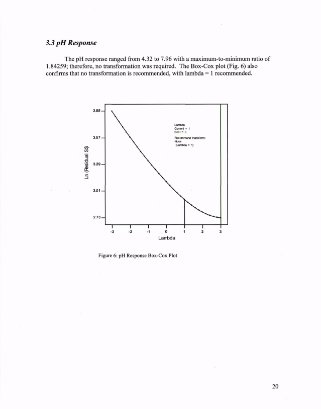
3.3 pH Response 20
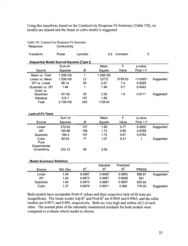
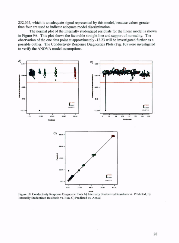
3.4 Conductivity Response 24
3.5 Dissolved Oxygen Response 33
3.6 Density Response 41
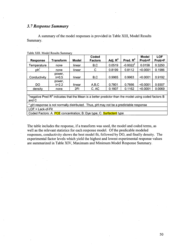
3.7 Response Summary 50
4.0 Discussion 55
4.1 Conductivity Response 55
4.2 Dissolved Oxygen Response 56
4.3 Implications to Geophysical Methods 56
5.0 Conclusions and Implications 60
6.0 Acknowledgements 61
7.0 References 62
Appendix A: QA/QC Protocols and Instrument Calibration Procedures 66
Appendix B: Standard Operating Procedure pH Meter 74
Appendix C: Standard Operating Procedure Conductivity Meter 83
Appendix D: Standard Operating Procedure Dissolved Oxygen Meter 92
Appendix E: Meter Calibration Data for QA Verification 100
Appendix F: PCE Concentration Sample Data for QA Verification 103
Appendix G: Cook's Distance 106
Appendix H: Glossary of Terms and Equations..' 108
Appendix I: Oil-Red-O Molecular Structure 113
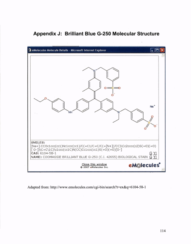
Appendix!: Brilliant Blue G-250 Molecular Structure 114
Appendix K: Experimental Factor Properties 115
11
image:
Table of Contents
Executive Summary i
Disclaimer i
Table of Contents ii
List of Figures iii
List of Tables iii
Appendices '. iv
1.0 Introduction 1
2.0 Methodology 5
2.1 Experimental Set-up and Procedures 8
2.2 Quality Assurance / Quality Control 8
2.2.1 Temperature Measurements 8
2.2.2 pH Measurements 9
2.2.3 Conductivity Measurements 9
2.2.4 Dissolved Oxygen Measurements 9
2.2.5 Density Measurements 10
2.2.6 GC/MS Volatile Compound Analyses 10
3.0 Results and Analysis 10
3.1 Quality Assurance / Quality Control 10
3.2 Temperature Response 11
3.3 pH Response 20
3.4 Conductivity Response 24
3.5 Dissolved Oxygen Response 33
3.6 Density Response 41
3.7 Response Summary 50
4.0 Discussion 55
4.1 Conductivity Response 55
4.2 Dissolved Oxygen Response 56
4.3 Implications to Geophysical Methods 56
5.0 Conclusions and Implications 60
6.0 Acknowledgements 61
7.0 References 62
Appendix A: QA/QC Protocols and Instrument Calibration Procedures 66
Appendix B: Standard Operating Procedure pH Meter 74
Appendix C: Standard Operating Procedure Conductivity Meter 83
Appendix D: Standard Operating Procedure Dissolved Oxygen Meter 92
Appendix E: Meter Calibration Data for QA Verification 100
Appendix F: PCE Concentration Sample Data for QA Verification 103
Appendix G: Cook's Distance 106
Appendix H: Glossary of Terms and Equations..' 108
Appendix I: Oil-Red-O Molecular Structure 113
Appendix!: Brilliant Blue G-250 Molecular Structure 114
Appendix K: Experimental Factor Properties 115
11
image:
 List of Figures
1. Temperature Response Box-Cox Plot
2. Temperature Response Diagnostics
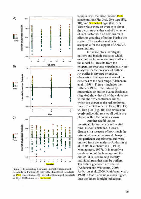
3. Temperature Response Residuals vs. Factors
4. Temperature Response Influence Plots
5. Temperature Response Dye vs. Surfactant at PCE Concentration =100 ppm
6. pH Box-Cox Plot for Power Transforms
7. pH Response Diagnostics
8. Conductivity Response Box-Cox Plot
9. Conductivity Normal Plot of Residuals: Linear and Cubic Model
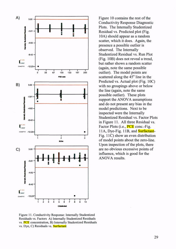
10. Conductivity Response Diagnostics Plots
11. Conductivity Response Residuals vs. Factors
12. Conductivity Response Influence Plots
13. Conductivity Model Response Plots
14. Dissolved Oxygen Box-Cox Plot for Power Transforms
15. Dissolved Oxygen Response Diagnostic Plots
16. Dissolved Oxygen Response Residual vs. Factors
17. Dissolved Oxygen Response Influence Plots
18. Dissolved Oxygen Model Response Plots
19. Density Response Box-Cox Plot
20. Density Diagnostic Plots
21. Density Response Residuals vs. Factors
22. Density Response Influence Plots
23. Density Response Plot
List of Tables
I. Surfactants and Experimental Concentrations
II. Experimental Design Summary
III. Temperature Response Fit Summary
IV. Temperature Response ANOVA
V. pH Response Fit Summary
VI. pH Response ANOVA
VII. Conductivity Response Fit Summary
VIII. Conductivity Response ANOVA
DC. Dissolved Oxygen Response Fit Summary
X. Dissolved Oxygen Response ANOVA
XL Density Response Fit Summary
XII. Density Response ANOVA
XIII. Results Summary
XIV. Maximum and Minimum Modeled Response Summary
XV. Conductivity Model Response in Ascending Order
XVI. Dissolved Oxygen Model Response in Ascending Order
in
image:
List of Figures
1. Temperature Response Box-Cox Plot
2. Temperature Response Diagnostics
3. Temperature Response Residuals vs. Factors
4. Temperature Response Influence Plots
5. Temperature Response Dye vs. Surfactant at PCE Concentration =100 ppm
6. pH Box-Cox Plot for Power Transforms
7. pH Response Diagnostics
8. Conductivity Response Box-Cox Plot
9. Conductivity Normal Plot of Residuals: Linear and Cubic Model
10. Conductivity Response Diagnostics Plots
11. Conductivity Response Residuals vs. Factors
12. Conductivity Response Influence Plots
13. Conductivity Model Response Plots
14. Dissolved Oxygen Box-Cox Plot for Power Transforms
15. Dissolved Oxygen Response Diagnostic Plots
16. Dissolved Oxygen Response Residual vs. Factors
17. Dissolved Oxygen Response Influence Plots
18. Dissolved Oxygen Model Response Plots
19. Density Response Box-Cox Plot
20. Density Diagnostic Plots
21. Density Response Residuals vs. Factors
22. Density Response Influence Plots
23. Density Response Plot
List of Tables
I. Surfactants and Experimental Concentrations
II. Experimental Design Summary
III. Temperature Response Fit Summary
IV. Temperature Response ANOVA
V. pH Response Fit Summary
VI. pH Response ANOVA
VII. Conductivity Response Fit Summary
VIII. Conductivity Response ANOVA
DC. Dissolved Oxygen Response Fit Summary
X. Dissolved Oxygen Response ANOVA
XL Density Response Fit Summary
XII. Density Response ANOVA
XIII. Results Summary
XIV. Maximum and Minimum Modeled Response Summary
XV. Conductivity Model Response in Ascending Order
XVI. Dissolved Oxygen Model Response in Ascending Order
in
image:
 Appendices
Appendix A. QA/QC Protocols and Instrument Calibration Procedures
Appendix B. Standard Operating Procedure pH Meter
Appendix C. Standard Operating Procedure Conductivity Meter
Appendix D. Standard Operating Procedure Dissolved Oxygen Meter
Appendix E. Meter Calibration Data for QA Verification
Appendix F. PCE Concentration Sample Data for QA Verification
Appendix G. Cook's Distance
Appendix H. Glossary of Terms and Equations
Appendix I. Brilliant Blue Molecular Structure
Appendix J. Oil-Red-O Molecular Structure
Appendix K. Experimental Factor Properties
IV
image:
Appendices
Appendix A. QA/QC Protocols and Instrument Calibration Procedures
Appendix B. Standard Operating Procedure pH Meter
Appendix C. Standard Operating Procedure Conductivity Meter
Appendix D. Standard Operating Procedure Dissolved Oxygen Meter
Appendix E. Meter Calibration Data for QA Verification
Appendix F. PCE Concentration Sample Data for QA Verification
Appendix G. Cook's Distance
Appendix H. Glossary of Terms and Equations
Appendix I. Brilliant Blue Molecular Structure
Appendix J. Oil-Red-O Molecular Structure
Appendix K. Experimental Factor Properties
IV
image:
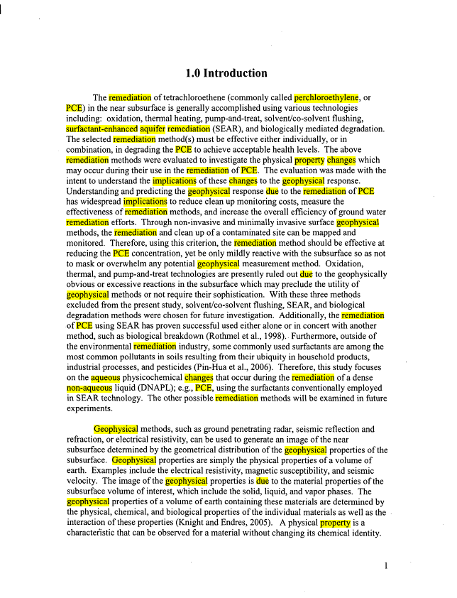
 1.0 Introduction
The remediation of tetrachloroethene (commonly called perchloroethylene, or
PCE) in the near subsurface is generally accomplished using various technologies
including: oxidation, thermal heating, pump-and-treat, solvent/co-solvent flushing,
surfactant-enhanced aquifer remediation (SEAR), and biologically mediated degradation.
The selected remediation method(s) must be effective either individually, or in
combination, in degrading the PCE to achieve acceptable health levels. The above
remediation methods were evaluated to investigate the physical property changes which
may occur during their use in the remediation of PCE. The evaluation was made with the
intent to understand the implications of these changes to the geophysical response.
Understanding and predicting the geophysical response due to the remediation of PCE
has widespread implications to reduce clean up monitoring costs, measure the
effectiveness of remediation methods, and increase the overall efficiency of ground water
remediation efforts. Through non-invasive and minimally invasive surface geophysical
methods, the remediation and clean up of a contaminated site can be mapped and
monitored. Therefore, using this criterion, the remediation method should be effective at
reducing the PCE concentration, yet be only mildly reactive with the subsurface so as not
to mask or overwhelm any potential geophysical measurement method. Oxidation,
thermal, and pump-and-treat technologies are presently ruled out due to the geophysically
obvious or excessive reactions in the subsurface which may preclude the utility of
geophysical methods or not require their sophistication. With these three methods
excluded from the present study, solvent/co-solvent flushing, SEAR, and biological
degradation methods were chosen for future investigation. Additionally, the remediation
of PCE using SEAR has proven successful used either alone or in concert with another
method, such as biological breakdown (Rothmel et al., 1998). Furthermore, outside of
the environmental remediation industry, some commonly used surfactants are among the
most common pollutants in soils resulting from their ubiquity in household products,
industrial processes, and pesticides (Pin-Hua et al., 2006). Therefore, this study focuses
on the aqueous physicochemical changes that occur during the remediation of a dense
non-aqueous liquid (DNAPL); e.g., PCE, using the surfactants conventionally employed
in SEAR technology. The other possible remediation methods will be examined in future
experiments.
Geophysical methods, such as ground penetrating radar, seismic reflection and
refraction, or electrical resistivity, can be used to generate an image of the near
subsurface determined by the geometrical distribution of the geophysical properties of the
subsurface. Geophysical properties are simply the physical properties of a volume of
earth. Examples include the electrical resistivity, magnetic susceptibility, and seismic
velocity. The image of the geophysical properties is due to the material properties of the
subsurface volume of interest, which include the solid, liquid, and vapor phases. The
geophysical properties of a volume of earth containing these materials are determined by
the physical, chemical, and biological properties of the individual materials as well as the
interaction of these properties (Knight and Endres, 2005). A physical property is a
characteristic that can be observed for a material without changing its chemical identity.
image:
1.0 Introduction
The remediation of tetrachloroethene (commonly called perchloroethylene, or
PCE) in the near subsurface is generally accomplished using various technologies
including: oxidation, thermal heating, pump-and-treat, solvent/co-solvent flushing,
surfactant-enhanced aquifer remediation (SEAR), and biologically mediated degradation.
The selected remediation method(s) must be effective either individually, or in
combination, in degrading the PCE to achieve acceptable health levels. The above
remediation methods were evaluated to investigate the physical property changes which
may occur during their use in the remediation of PCE. The evaluation was made with the
intent to understand the implications of these changes to the geophysical response.
Understanding and predicting the geophysical response due to the remediation of PCE
has widespread implications to reduce clean up monitoring costs, measure the
effectiveness of remediation methods, and increase the overall efficiency of ground water
remediation efforts. Through non-invasive and minimally invasive surface geophysical
methods, the remediation and clean up of a contaminated site can be mapped and
monitored. Therefore, using this criterion, the remediation method should be effective at
reducing the PCE concentration, yet be only mildly reactive with the subsurface so as not
to mask or overwhelm any potential geophysical measurement method. Oxidation,
thermal, and pump-and-treat technologies are presently ruled out due to the geophysically
obvious or excessive reactions in the subsurface which may preclude the utility of
geophysical methods or not require their sophistication. With these three methods
excluded from the present study, solvent/co-solvent flushing, SEAR, and biological
degradation methods were chosen for future investigation. Additionally, the remediation
of PCE using SEAR has proven successful used either alone or in concert with another
method, such as biological breakdown (Rothmel et al., 1998). Furthermore, outside of
the environmental remediation industry, some commonly used surfactants are among the
most common pollutants in soils resulting from their ubiquity in household products,
industrial processes, and pesticides (Pin-Hua et al., 2006). Therefore, this study focuses
on the aqueous physicochemical changes that occur during the remediation of a dense
non-aqueous liquid (DNAPL); e.g., PCE, using the surfactants conventionally employed
in SEAR technology. The other possible remediation methods will be examined in future
experiments.
Geophysical methods, such as ground penetrating radar, seismic reflection and
refraction, or electrical resistivity, can be used to generate an image of the near
subsurface determined by the geometrical distribution of the geophysical properties of the
subsurface. Geophysical properties are simply the physical properties of a volume of
earth. Examples include the electrical resistivity, magnetic susceptibility, and seismic
velocity. The image of the geophysical properties is due to the material properties of the
subsurface volume of interest, which include the solid, liquid, and vapor phases. The
geophysical properties of a volume of earth containing these materials are determined by
the physical, chemical, and biological properties of the individual materials as well as the
interaction of these properties (Knight and Endres, 2005). A physical property is a
characteristic that can be observed for a material without changing its chemical identity.
image:
 A chemical property, on the other hand, is only observed by changing a substance's
chemical identity, and a biological property can be determined by the organism's activity.
Physical property attributes include the electrical conductivity, temperature, density,
dielectric, and acoustic properties. Geophysical methods measure these physical
properties due to the bulk response of the subsurface volume, which includes the solid,
liquid, and gas portions as well as the chemical and biological interactions. In
applications of geophysics to contaminant and remediation efforts, the geologic material
in which the contaminant (e.g., PCE) exists and into which the remediation method (e.g.,
SEAR) would be introduced impacts the geophysical response because the physical,
chemical, and biological properties of the subsurface are altered. In addition, the
components of the geologic media involve several levels of complexity. First, the
geologic media itself generates a geophysical response as a result of the specific physical
properties of the solid material. Second, the interaction between the geologic media and
natural subsurface fluids and their specific properties (e.g., pH) adds another component
of the geophysical response. Additionally, any contaminate will interact with the natural
subsurface solid and liquid phases and result in changes to the measured geophysical
system. Evaluation of the geophysical response with multiple geologic and groundwater
conditions, a range of PCE concentrations, and varying surfactant treatments, presents a
very complex investigation. Therefore, as an initial investigation and to simplify the
potential reactions and interactions between the different media, this project focuses on
changes only in the aqueous phase. The experiments are designed to provide a predictive
model for select aqueous phase properties due to the surfactant remediation of PCE.
Much work has been done on the use of surfactants to both solubilize and
mobilize PCE (Conrad et al., 2002; Dwarakanath et al., 1999; Londergan et al, 2001;
McGuire and Hughes, 2003; Rommel et al., 1998; Sabatini et al., 1996; Taylor et al.,
2004; West and Harwell, 1992). Briefly, SEAR involves the injection of surfactants into
the subsurface to recover NAPL-contaminants by either enhanced solubilization or
mobilization due to interfacial tension reduction. Surfactants are surface active agents
(Sabatini et al., 1995) the molecules of which are composed of a hydrophilic tail and a
hydrophobic head. This results in the molecule's behavior in the formation of
microemulsions. Microemulsions are thermodynamically stable and swollen micellular
solutions. Surfactants may be cationic, nonionic, anionic, or zwitterionic. The use of
anionic surfactants is the most common because these tend not to adsorb (because of like
charges) to native negatively charged subsurface solid material as do cationic types
(Dwarakanath et al., 1999). Zwitterionic surfactants are rarely used in the field for
remediation. Surfactants that disrupt structure are best for microemulsions of DNAPLs.
Surfactants used for remediation can be engineered such that the optimization of the
surfactant for performance does not create another environmental problem. The use of
surfactants has resulted in greater than 99% contaminant removal in soil columns
(Dwarakanath and Pope, 2000), 96.9% in other soil column studies (Sabatini et al., 2000),
98.5 % DNAPL removed from an alluvial aquifer (Londergan et al., 2001), 90% recovery
of PCE in bench scale studies (Conrad et al., 2002), and 97% PCE extraction in others
(Sabatini et al., 1996). For this project, nine surfactants (factor coded C) were selected
for experimentation, as determined from those most prevalently used, and those which
contained the two primary charge types, nonionic and anionic. The surfactant 4% Tween
image:
A chemical property, on the other hand, is only observed by changing a substance's
chemical identity, and a biological property can be determined by the organism's activity.
Physical property attributes include the electrical conductivity, temperature, density,
dielectric, and acoustic properties. Geophysical methods measure these physical
properties due to the bulk response of the subsurface volume, which includes the solid,
liquid, and gas portions as well as the chemical and biological interactions. In
applications of geophysics to contaminant and remediation efforts, the geologic material
in which the contaminant (e.g., PCE) exists and into which the remediation method (e.g.,
SEAR) would be introduced impacts the geophysical response because the physical,
chemical, and biological properties of the subsurface are altered. In addition, the
components of the geologic media involve several levels of complexity. First, the
geologic media itself generates a geophysical response as a result of the specific physical
properties of the solid material. Second, the interaction between the geologic media and
natural subsurface fluids and their specific properties (e.g., pH) adds another component
of the geophysical response. Additionally, any contaminate will interact with the natural
subsurface solid and liquid phases and result in changes to the measured geophysical
system. Evaluation of the geophysical response with multiple geologic and groundwater
conditions, a range of PCE concentrations, and varying surfactant treatments, presents a
very complex investigation. Therefore, as an initial investigation and to simplify the
potential reactions and interactions between the different media, this project focuses on
changes only in the aqueous phase. The experiments are designed to provide a predictive
model for select aqueous phase properties due to the surfactant remediation of PCE.
Much work has been done on the use of surfactants to both solubilize and
mobilize PCE (Conrad et al., 2002; Dwarakanath et al., 1999; Londergan et al, 2001;
McGuire and Hughes, 2003; Rommel et al., 1998; Sabatini et al., 1996; Taylor et al.,
2004; West and Harwell, 1992). Briefly, SEAR involves the injection of surfactants into
the subsurface to recover NAPL-contaminants by either enhanced solubilization or
mobilization due to interfacial tension reduction. Surfactants are surface active agents
(Sabatini et al., 1995) the molecules of which are composed of a hydrophilic tail and a
hydrophobic head. This results in the molecule's behavior in the formation of
microemulsions. Microemulsions are thermodynamically stable and swollen micellular
solutions. Surfactants may be cationic, nonionic, anionic, or zwitterionic. The use of
anionic surfactants is the most common because these tend not to adsorb (because of like
charges) to native negatively charged subsurface solid material as do cationic types
(Dwarakanath et al., 1999). Zwitterionic surfactants are rarely used in the field for
remediation. Surfactants that disrupt structure are best for microemulsions of DNAPLs.
Surfactants used for remediation can be engineered such that the optimization of the
surfactant for performance does not create another environmental problem. The use of
surfactants has resulted in greater than 99% contaminant removal in soil columns
(Dwarakanath and Pope, 2000), 96.9% in other soil column studies (Sabatini et al., 2000),
98.5 % DNAPL removed from an alluvial aquifer (Londergan et al., 2001), 90% recovery
of PCE in bench scale studies (Conrad et al., 2002), and 97% PCE extraction in others
(Sabatini et al., 1996). For this project, nine surfactants (factor coded C) were selected
for experimentation, as determined from those most prevalently used, and those which
contained the two primary charge types, nonionic and anionic. The surfactant 4% Tween
image:
 80, a polyoxyethylene-20-sorbitan monooleate is nonionic. This surfactant, both alone
and with 10% EtOH, has been used by many researchers (McGuire and Hughes, 2003;
Ramsburg and Pennell, 2000; Taylor et al., 2004) and was chosen due to its prevalence,
nonionic characteristics, and its efficacy at PCE removal. In addition, it has been used
with the two dye types employed in this experiment as described below. Fifty mM
Tween 60, a polyoxyethylene-20-sorbitan monostearate, is also nonionic and has shown
good solubilization of PCE (Sabatini et al., 1996). The surfactant 0.5% AMA-80-I is a
low concentration of the anionic sodium dihexyl sulfosuccinate and was found to
successfully solubilize PCE without producing a false PCE saturation in column
experiments (Cho et al., 2004). A higher concentration of approximately'8% AMA-80-I
was shown to successfully remove PCE by two orders of magnitude in a field study
(Londergan et al., 2001). Steol CS-330 is the anionic sodium laureth sulfate + alcohol
ethoxylate and was used at 0.025% and 0.10% concentrations. The levels of Steol CS-
330 were included because they were shown to emulsify trichloroethylene (TCE) and
were biocompatible with a bio-variant, ENV-435, which is very specialized and can
degrade TCE (Rothmel et al., 1998). Cho et al., (2004) also investigated 0.5% and 5%
Dowfax 8390 in batch and column experiments to detect the magnitude of artifacts
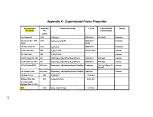
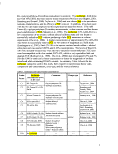
introduced while estimating DNAPL content. In summary, Table I shows the ten
surfactant categories used in this study, their respective experimental factor code,
components and concentration, ionic type, and the source reference.
Table I: Surfactants and Experimental Concentrations
Coded
Factor
Cl
C2
C3
C4
C5
C6
C7
C8
C9
CIO
Surfactant
concentration (w/w)
in DI water
4% Tween 80
4% Tween 80 +10%
EtOH
50 mM Tween 60
0.5% AMA-80-I
8% AMA-80-I
0.025% Steol CS-330
0.10% Steol CS-330
0.5% Dowfax 8390
5% Dowfax 8390
No surfactant
Comments
Polyoxyethylene-20-
Sorbitan monooleate
Polyoxyethylene-20-
Sorbitan monostearate
Sodium dihexyl
sulfosuccinate
Sodium laureth sulfate +
Alcohol ethoxylate
Sodium hexadecyl
diphenyl oxide +
Disodium
dihexyldecyldiphenyl
oxide + Sodium sulfate
—
Charge type
nonionic
anionic
—
Reference
Taylor et al., 2004
Ramsburg and
Pennell, 2000;
Taylor et al., 2004
Sabatina et al., 1996
Cho et al., 2004
Londergan et al.,
2001; Ramsburg
and Pennell, 2000
Rothmel et al., 1998
Rothmel et al., 1998
Cho et al., 2004
Cho et al., 2004
....
image:
80, a polyoxyethylene-20-sorbitan monooleate is nonionic. This surfactant, both alone
and with 10% EtOH, has been used by many researchers (McGuire and Hughes, 2003;
Ramsburg and Pennell, 2000; Taylor et al., 2004) and was chosen due to its prevalence,
nonionic characteristics, and its efficacy at PCE removal. In addition, it has been used
with the two dye types employed in this experiment as described below. Fifty mM
Tween 60, a polyoxyethylene-20-sorbitan monostearate, is also nonionic and has shown
good solubilization of PCE (Sabatini et al., 1996). The surfactant 0.5% AMA-80-I is a
low concentration of the anionic sodium dihexyl sulfosuccinate and was found to
successfully solubilize PCE without producing a false PCE saturation in column
experiments (Cho et al., 2004). A higher concentration of approximately'8% AMA-80-I
was shown to successfully remove PCE by two orders of magnitude in a field study
(Londergan et al., 2001). Steol CS-330 is the anionic sodium laureth sulfate + alcohol
ethoxylate and was used at 0.025% and 0.10% concentrations. The levels of Steol CS-
330 were included because they were shown to emulsify trichloroethylene (TCE) and
were biocompatible with a bio-variant, ENV-435, which is very specialized and can
degrade TCE (Rothmel et al., 1998). Cho et al., (2004) also investigated 0.5% and 5%
Dowfax 8390 in batch and column experiments to detect the magnitude of artifacts
introduced while estimating DNAPL content. In summary, Table I shows the ten
surfactant categories used in this study, their respective experimental factor code,
components and concentration, ionic type, and the source reference.
Table I: Surfactants and Experimental Concentrations
Coded
Factor
Cl
C2
C3
C4
C5
C6
C7
C8
C9
CIO
Surfactant
concentration (w/w)
in DI water
4% Tween 80
4% Tween 80 +10%
EtOH
50 mM Tween 60
0.5% AMA-80-I
8% AMA-80-I
0.025% Steol CS-330
0.10% Steol CS-330
0.5% Dowfax 8390
5% Dowfax 8390
No surfactant
Comments
Polyoxyethylene-20-
Sorbitan monooleate
Polyoxyethylene-20-
Sorbitan monostearate
Sodium dihexyl
sulfosuccinate
Sodium laureth sulfate +
Alcohol ethoxylate
Sodium hexadecyl
diphenyl oxide +
Disodium
dihexyldecyldiphenyl
oxide + Sodium sulfate
—
Charge type
nonionic
anionic
—
Reference
Taylor et al., 2004
Ramsburg and
Pennell, 2000;
Taylor et al., 2004
Sabatina et al., 1996
Cho et al., 2004
Londergan et al.,
2001; Ramsburg
and Pennell, 2000
Rothmel et al., 1998
Rothmel et al., 1998
Cho et al., 2004
Cho et al., 2004
....
image:
 The second factor (coded B) investigated in this experiment was the use of dyes
for visually tracking PCE migration and movement in the subsurface. Because PCE is a
clear liquid, visual observations of subsurface migration is very difficult. As a result,
investigators have used PCE-soluble dyes to observe subsurface PCE migration in
laboratory experiments (Jeong et al., 2002; Longino and Kueper, 1994; Taylor et al.,
2001). Two conservative and non-reactive dyes were used: Oil-Red-O and Brilliant
Blue-G250 each at a concentration of 10"4 Molar (Jeong et al., 2002; Taylor et al., 2001;
Taylor et al., 2004). Taylor et al., (2001) showed that this concentration of Oil-Red-O
has no significant effect on the solubilization, interfacial tension, and viscosity of PCE.
Other research shows that the presence of Oil-Red-O does alter the interfacial tension
between PCE and water or PCE and ethanol solutions (Jeong et al., 2002; Longino and
Kueper, 1994). Furthermore, the DNAPL migration into porous media is altered due to
the effect of altering the surface tension of PCE (Jeong et al., 2002). Further research
found that dye use increases DNAPL surface chemical complexity and increases PCE
mobility through lower adhesion tension (Tuck and Iversen, 2003). To determine if the
use of these dyes results in changes to the responses measured, dye type was included as
a categorical (nominal) factor in this experimental design. The three dye type categories
were none, Oil-Red-O, and Brilliant Blue-G250.
The final experimental factor (coded A) was PCE concentration. Surfactant
remediation of PCE is typically utilized for residual or saturated PCE concentrations.
Free-phase PCE is typically treated with other technologies. Furthermore, the laboratory
equipment utilized in these experiments is not robust enough to withstand free-phase
concentrations of PCE. Therefore, the highest concentration of PCE was its aqueous
solubility at room temperature (25°C), 200 ppm (NIOSH, 1994). A total of five PCE
concentrations were used to occupy the design space: 0, 50, 100, 150, and 200 ppm PCE.
Thus, the objective of this initial phase of the research was to determine the
relationship of the temperature, conductivity, dissolved oxygen, pH, and density of the
aqueous solution as a function of surfactant type, PCE concentration, and dye type. The
evaluation of the resulting aqueous properties will provide an initial understanding of the
potential geophysical response to the SEAR of PCE.
image:
The second factor (coded B) investigated in this experiment was the use of dyes
for visually tracking PCE migration and movement in the subsurface. Because PCE is a
clear liquid, visual observations of subsurface migration is very difficult. As a result,
investigators have used PCE-soluble dyes to observe subsurface PCE migration in
laboratory experiments (Jeong et al., 2002; Longino and Kueper, 1994; Taylor et al.,
2001). Two conservative and non-reactive dyes were used: Oil-Red-O and Brilliant
Blue-G250 each at a concentration of 10"4 Molar (Jeong et al., 2002; Taylor et al., 2001;
Taylor et al., 2004). Taylor et al., (2001) showed that this concentration of Oil-Red-O
has no significant effect on the solubilization, interfacial tension, and viscosity of PCE.
Other research shows that the presence of Oil-Red-O does alter the interfacial tension
between PCE and water or PCE and ethanol solutions (Jeong et al., 2002; Longino and
Kueper, 1994). Furthermore, the DNAPL migration into porous media is altered due to
the effect of altering the surface tension of PCE (Jeong et al., 2002). Further research
found that dye use increases DNAPL surface chemical complexity and increases PCE
mobility through lower adhesion tension (Tuck and Iversen, 2003). To determine if the
use of these dyes results in changes to the responses measured, dye type was included as
a categorical (nominal) factor in this experimental design. The three dye type categories
were none, Oil-Red-O, and Brilliant Blue-G250.
The final experimental factor (coded A) was PCE concentration. Surfactant
remediation of PCE is typically utilized for residual or saturated PCE concentrations.
Free-phase PCE is typically treated with other technologies. Furthermore, the laboratory
equipment utilized in these experiments is not robust enough to withstand free-phase
concentrations of PCE. Therefore, the highest concentration of PCE was its aqueous
solubility at room temperature (25°C), 200 ppm (NIOSH, 1994). A total of five PCE
concentrations were used to occupy the design space: 0, 50, 100, 150, and 200 ppm PCE.
Thus, the objective of this initial phase of the research was to determine the
relationship of the temperature, conductivity, dissolved oxygen, pH, and density of the
aqueous solution as a function of surfactant type, PCE concentration, and dye type. The
evaluation of the resulting aqueous properties will provide an initial understanding of the
potential geophysical response to the SEAR of PCE.
image:
 2.0 Methodology
The response surface methods (RSM) for experimental design is typically used
for product process enhancement or the identification of the high plateaus or peaks of
product quality or process efficiency (Anderson and Whitcomb, 2000; Anderson and
Whitcomb, 2005). The RSM includes mathematical and statistical techniques used for
modeling and analysis of problems involving a response of interest which is influenced
by several variables where the objective is to optimize the response (Montgomery, 1997).
This methodology has had much success in industrial applications and the application of
RSM to physicochemical property changes in an aqueous solution utilizes the same
mathematics, but with a different frame of reference. For example, Montgomery (1997)
uses the example of a chemical engineer trying to maximize the yield (y) of a process,
which is dependent upon the levels of temperature (xi) and pressure (x2). The yield is,
therefore, a function of the levels of the temperature and pressure, such that;
y = f(xltx2)+e
where £ is the noise, error, or uncertainty observed in the response. Montgomery (1997)
goes on to suggest denoting the expected response as E(y) =flxi,\2~) = rj. Therefore, the
surface represented by TJ = f(x},x2) is termed a response surface (Montgomery, 1997).
The application of the RSM to the response prediction of aqueous properties is a direct
analogue to the industrial application and can be thought of as maximizing or optimizing
the response, conductivity, for example, due to certain factors or factor interactions. The
RSM was used in this application to model the dependent variable or responses, in this
case, the particular aqueous property (i.e., temperature, pH, conductivity, dissolved
oxygen, or density) due to the factors: PCE concentration, dye type, surfactant type, or
the interaction of these factors. In terms of the example above given by Montgomery
(1997), the yield (yi) would be the responses, or in our case, the aqueous properties where
i= temperature, pH, conductivity, dissolved oxygen, or density. The factors (xk) are the
independent variables where k=PCE concentration, dye type, surfactant type, or the
interactions of these factors. Therefore, the RSM experimental design was chosen to
provide a response surface to navigate the experimental space and determine the response
(yi) per each factor or factor interaction (xk). If the three experimental factors are
significant to the particular response and the particular model assumptions are valid, then
each of the five responses will produce a response as a function of the three experimental
factors. Further details of the response surface method in experimental design can be
found in several sources (Anderson and Whitcomb, 2005; Montgomery, 1997).
The summary of the design is as follows. The three factors are coded A, B, and
C. A is PCE concentration, B is dye type, and C is surfactant type. PCE type is a
numeric factor with concentrations of 0, 50, 100, 150, and 200 ppm, the latter being the
top limit of the aqueous solubility of PCE at 25°C (NIOSH, 1994). Dye type is a nominal
categorical factor with three levels: none or no dye, Oil-Red-O (Solvent Red 27, formula
weight = 408.5), and Brilliant Blue-G 250 (FW = 854.02). The dyes are added to the
experimental solutions to achieve a final concentration of 10"4 Molar. Surfactant type is
also a nominal categorical factor with 10 levels as described in Table I. The RSM design
image:
2.0 Methodology
The response surface methods (RSM) for experimental design is typically used
for product process enhancement or the identification of the high plateaus or peaks of
product quality or process efficiency (Anderson and Whitcomb, 2000; Anderson and
Whitcomb, 2005). The RSM includes mathematical and statistical techniques used for
modeling and analysis of problems involving a response of interest which is influenced
by several variables where the objective is to optimize the response (Montgomery, 1997).
This methodology has had much success in industrial applications and the application of
RSM to physicochemical property changes in an aqueous solution utilizes the same
mathematics, but with a different frame of reference. For example, Montgomery (1997)
uses the example of a chemical engineer trying to maximize the yield (y) of a process,
which is dependent upon the levels of temperature (xi) and pressure (x2). The yield is,
therefore, a function of the levels of the temperature and pressure, such that;
y = f(xltx2)+e
where £ is the noise, error, or uncertainty observed in the response. Montgomery (1997)
goes on to suggest denoting the expected response as E(y) =flxi,\2~) = rj. Therefore, the
surface represented by TJ = f(x},x2) is termed a response surface (Montgomery, 1997).
The application of the RSM to the response prediction of aqueous properties is a direct
analogue to the industrial application and can be thought of as maximizing or optimizing
the response, conductivity, for example, due to certain factors or factor interactions. The
RSM was used in this application to model the dependent variable or responses, in this
case, the particular aqueous property (i.e., temperature, pH, conductivity, dissolved
oxygen, or density) due to the factors: PCE concentration, dye type, surfactant type, or
the interaction of these factors. In terms of the example above given by Montgomery
(1997), the yield (yi) would be the responses, or in our case, the aqueous properties where
i= temperature, pH, conductivity, dissolved oxygen, or density. The factors (xk) are the
independent variables where k=PCE concentration, dye type, surfactant type, or the
interactions of these factors. Therefore, the RSM experimental design was chosen to
provide a response surface to navigate the experimental space and determine the response
(yi) per each factor or factor interaction (xk). If the three experimental factors are
significant to the particular response and the particular model assumptions are valid, then
each of the five responses will produce a response as a function of the three experimental
factors. Further details of the response surface method in experimental design can be
found in several sources (Anderson and Whitcomb, 2005; Montgomery, 1997).
The summary of the design is as follows. The three factors are coded A, B, and
C. A is PCE concentration, B is dye type, and C is surfactant type. PCE type is a
numeric factor with concentrations of 0, 50, 100, 150, and 200 ppm, the latter being the
top limit of the aqueous solubility of PCE at 25°C (NIOSH, 1994). Dye type is a nominal
categorical factor with three levels: none or no dye, Oil-Red-O (Solvent Red 27, formula
weight = 408.5), and Brilliant Blue-G 250 (FW = 854.02). The dyes are added to the
experimental solutions to achieve a final concentration of 10"4 Molar. Surfactant type is
also a nominal categorical factor with 10 levels as described in Table I. The RSM design
image:
 of choice is the one numerical factor RSM design. The number of levels required of the
numerical factor determines the order of the polynomial. In this case, five levels of a
single factor (i.e., PCE at the levels indicated above), plus replicates, allow a lack-of-fit
analysis (see Appendix H for definition) and a purely experimental uncertainty
determination for a quadratic model. Additionally, this RSM design allows the addition
of categorical factors (Stat-Ease, 2006). Therefore, this investigation is designed with a
response surface methodology quadratic design model with no blocking. Blocking is a
technique which can be used to remove the expected variation caused by some change
during the course of the experiment. A general rule of thumb for blocking is to only
block on a factor that one is not interested in studying (the block is aliased with the
chosen, usually insignificant, factor, which is usually a high order interaction). No
blocking was chosen for this experiment. Per the RSM experimental quadratic design
model 240 experimental runs were performed, which is determined from 1 numeric
factor, A at 5 levels, 2 nominal categorical factors; B at 3 levels and C at 10 levels, with
duplication for every combination of the categorical factor levels, and with 60 center
points. The five responses measured were: temperature (°C), conductivity (fiS/cm),
dissolved oxygen (DO, mg/L), pH, and density (g/mL). The experimental design was set
up using Design Expert v7 from Stat-Ease, Inc. (Stat-Ease, 2006). The software sets up
the randomized run order and replicates as necessary per the model design. The
experimental design is summarized in Table II.
image:
of choice is the one numerical factor RSM design. The number of levels required of the
numerical factor determines the order of the polynomial. In this case, five levels of a
single factor (i.e., PCE at the levels indicated above), plus replicates, allow a lack-of-fit
analysis (see Appendix H for definition) and a purely experimental uncertainty
determination for a quadratic model. Additionally, this RSM design allows the addition
of categorical factors (Stat-Ease, 2006). Therefore, this investigation is designed with a
response surface methodology quadratic design model with no blocking. Blocking is a
technique which can be used to remove the expected variation caused by some change
during the course of the experiment. A general rule of thumb for blocking is to only
block on a factor that one is not interested in studying (the block is aliased with the
chosen, usually insignificant, factor, which is usually a high order interaction). No
blocking was chosen for this experiment. Per the RSM experimental quadratic design
model 240 experimental runs were performed, which is determined from 1 numeric
factor, A at 5 levels, 2 nominal categorical factors; B at 3 levels and C at 10 levels, with
duplication for every combination of the categorical factor levels, and with 60 center
points. The five responses measured were: temperature (°C), conductivity (fiS/cm),
dissolved oxygen (DO, mg/L), pH, and density (g/mL). The experimental design was set
up using Design Expert v7 from Stat-Ease, Inc. (Stat-Ease, 2006). The software sets up
the randomized run order and replicates as necessary per the model design. The
experimental design is summarized in Table II.
image:
 Table II: Experimental Design Summary
Response
Study Type: Surface Runs
Initial No
Design: One Factor Blocks
Design
Model: Quadratic
240
Factor
A
B
C
Response
Y1
Y2
Y3
Y4
Y5
Name
PCEconc
Dye
Surfactant
Name
Temp
Cond
DO
PH
density
Units
ppm
type
type
Units
degC
uS/cm
mg/L
-logio[H+]
g/mL
Type
Numeric
Categoric
Categoric
Obs
240
240
240
240
240
Low
Actual
0
none
4% Tween
80
Analysis
Polynomial
Polynomial
Polynomial
Polynomial
Polynomial
High
Actual
200
Oil-Red-O
No
Surfactant
Minimum
15.9
0.968
3.18
4.32
0.982
Low
Coded
-1
Maximum
21.7
7610
10.48
7.96
1.02267
High
Coded
1
Mean
19.0454167
1138.94047
7.85408333
5.954125
1.00272192
Mean
100
Levels:
Levels:
Std. Dev.
1.1600556
2174.7257
1.53E+00
0.6675228
0.007443
Std.
Dev.
75
3
10
Max./Min.
Ratio
1.36478
7861.57
3.295597
1.842593
1.041415
Transform
None
Power
Power
None
None
Model
RLinear
RLJnear
Linear
RLinear
R2FI
RLinear = reduced linear model
Linear = linear model
R2FI = reduced 2 factor interaction
image:
Table II: Experimental Design Summary
Response
Study Type: Surface Runs
Initial No
Design: One Factor Blocks
Design
Model: Quadratic
240
Factor
A
B
C
Response
Y1
Y2
Y3
Y4
Y5
Name
PCEconc
Dye
Surfactant
Name
Temp
Cond
DO
PH
density
Units
ppm
type
type
Units
degC
uS/cm
mg/L
-logio[H+]
g/mL
Type
Numeric
Categoric
Categoric
Obs
240
240
240
240
240
Low
Actual
0
none
4% Tween
80
Analysis
Polynomial
Polynomial
Polynomial
Polynomial
Polynomial
High
Actual
200
Oil-Red-O
No
Surfactant
Minimum
15.9
0.968
3.18
4.32
0.982
Low
Coded
-1
Maximum
21.7
7610
10.48
7.96
1.02267
High
Coded
1
Mean
19.0454167
1138.94047
7.85408333
5.954125
1.00272192
Mean
100
Levels:
Levels:
Std. Dev.
1.1600556
2174.7257
1.53E+00
0.6675228
0.007443
Std.
Dev.
75
3
10
Max./Min.
Ratio
1.36478
7861.57
3.295597
1.842593
1.041415
Transform
None
Power
Power
None
None
Model
RLinear
RLJnear
Linear
RLinear
R2FI
RLinear = reduced linear model
Linear = linear model
R2FI = reduced 2 factor interaction
image:
 2.1 Experimental Set-up and Procedures
Prior to determining the mechanics of the experimental procedures, preliminary
instrument calibrations and test analyses were undertaken to address'issues pertinent to the
procedures and the required data quality. These preliminary (i.e., familiarity) experiments
determined:
- the operational calibration range for each instrument,
- the range of drift in standard measurements over time and with fluctuating ambient
temperatures for each instrument,
— the optimal sample volume necessary to allow simultaneous measurements with
multiple instrument probes or electrodes,
- if the instrument probes or electrodes were negatively impacted by increasing levels of
PCE in the solutions,
- the general experimental characteristics of the surfactants to be used and if the
measurements would be expected to fall within the calibration ranges of the
instruments,
— the sequence of response measurements to assure that quality data was collected, and
- decontamination of probes and electrodes (i.e., no "carry-over" effects).
The results of these validation and calibration experiments defined the following
experimental procedures and Quality Assurance/Quality Control (QA/QC) protocols, the
details of which can be found in Werkema (2006). Each of the 240 experimental runs
would be performed in a 400 mL beaker by accurately measuring 300 mL of the matrix
(e.g. DI water or surfactant) under a hood to vent volatiles. PCE, dye (weighed out dry for
each beaker), and surfactant concentrations were determined volumetrically and introduced
to the beaker. A magnetic stir bar was used for mixing. Five minutes after the introduction
of the specific experimental treatment (i.e., independent variable) the responses (i.e.
dependent variables) were measured in the following order: temperature, conductivity, pH,
and DO. Density was then calculated through mass and volume measurements. To verify
the concentration of PCE measured into the beakers, an aliquot of each sample matrix
containing PCE were transferred to a labeled, pre-cleaned 40-mL glass vial with a Teflon-
lined, septum-sealed screw top (VOA vial) for analysis on the GC/MS. The volumes to be
sampled for each PCE concentration and the blank are listed in Table 3 of the QAPP
(Werkema, 2006). These measurements were used to verify the concentration of PCE or
breakdown products in the samples undergoing the electrochemical testing. This analysis
served as a quality assurance check for the treatments.
2.2 Quality Assurance / Quality Control
2.2.1 Temperature Measurements
Temperature resolution and accuracy for the two meters used are given as °C per
the instrument manufacturers. The Denver Instrument Electrochemistry Meter claims 0.1°
resolution, ± 0.3° accuracy (Denver Instrument Co., 1999) and the Accumet® Model AR 60
Meter: 0.1° resolution, ±0.1° accuracy (Fisher Scientific, 2003). The stand alone
temperature probe and pH electrode with Automatic Temperature Compensation (ATC),
image:
2.1 Experimental Set-up and Procedures
Prior to determining the mechanics of the experimental procedures, preliminary
instrument calibrations and test analyses were undertaken to address'issues pertinent to the
procedures and the required data quality. These preliminary (i.e., familiarity) experiments
determined:
- the operational calibration range for each instrument,
- the range of drift in standard measurements over time and with fluctuating ambient
temperatures for each instrument,
— the optimal sample volume necessary to allow simultaneous measurements with
multiple instrument probes or electrodes,
- if the instrument probes or electrodes were negatively impacted by increasing levels of
PCE in the solutions,
- the general experimental characteristics of the surfactants to be used and if the
measurements would be expected to fall within the calibration ranges of the
instruments,
— the sequence of response measurements to assure that quality data was collected, and
- decontamination of probes and electrodes (i.e., no "carry-over" effects).
The results of these validation and calibration experiments defined the following
experimental procedures and Quality Assurance/Quality Control (QA/QC) protocols, the
details of which can be found in Werkema (2006). Each of the 240 experimental runs
would be performed in a 400 mL beaker by accurately measuring 300 mL of the matrix
(e.g. DI water or surfactant) under a hood to vent volatiles. PCE, dye (weighed out dry for
each beaker), and surfactant concentrations were determined volumetrically and introduced
to the beaker. A magnetic stir bar was used for mixing. Five minutes after the introduction
of the specific experimental treatment (i.e., independent variable) the responses (i.e.
dependent variables) were measured in the following order: temperature, conductivity, pH,
and DO. Density was then calculated through mass and volume measurements. To verify
the concentration of PCE measured into the beakers, an aliquot of each sample matrix
containing PCE were transferred to a labeled, pre-cleaned 40-mL glass vial with a Teflon-
lined, septum-sealed screw top (VOA vial) for analysis on the GC/MS. The volumes to be
sampled for each PCE concentration and the blank are listed in Table 3 of the QAPP
(Werkema, 2006). These measurements were used to verify the concentration of PCE or
breakdown products in the samples undergoing the electrochemical testing. This analysis
served as a quality assurance check for the treatments.
2.2 Quality Assurance / Quality Control
2.2.1 Temperature Measurements
Temperature resolution and accuracy for the two meters used are given as °C per
the instrument manufacturers. The Denver Instrument Electrochemistry Meter claims 0.1°
resolution, ± 0.3° accuracy (Denver Instrument Co., 1999) and the Accumet® Model AR 60
Meter: 0.1° resolution, ±0.1° accuracy (Fisher Scientific, 2003). The stand alone
temperature probe and pH electrode with Automatic Temperature Compensation (ATC),
image:
 conductivity ATC, and DO ATC all measure temperature, and if the readings were not
within ± 2°C, then all three temperature readings were recorded. The average of these
three was used in the data analysis. Otherwise, a single reading was recorded from the
measurements.
2.2.2 pH Measurements
Measurements for pH were made according to SW-846 Method 9040C, pH
Electrometric Measurement (USEPA, 2004), and the laboratory Standard Operating
Procedure (SOP), pH Meter: Calibration and Measurements (see Appendix B). An
Accumet® glass-body, combination pH electrode with silver/silver chloride reference was
used for this procedure (Fisher Scientific, 2003). Temperature effects on the readings were
documented or mitigated by using a temperature probe with ATC in conjunction with the
measurements and recording the temperature as each reading was being made. The probes
were used with a Denver Instrument 200 Series Electrochemistry Meter, which is capable
of three-to-five-point calibrations and simultaneous readings of multiple parameters
(Denver Instrument Co., 1999).
2.2.3 Conductivity Measurements
Measurements for conductivity followed SW-846 Method 9050A, Specific
Conductance (USEPA, 1996), and the laboratory SOP, Conductivity Meter: Calibration
and Measurements (see Appendix C). A 4-cell, plastic-body probe and a 2-cell, glass-body
probe were used in this study. Both have a nominal cell constant of 1.0 cm"' and a
measurement range of 10.0- 2000 |iS/cm. The 2-cell probe was available for use with
samples containing high concentrations of PCE. The 4-cell probe has integrated ATC
capacity, and was used with the Denver Instrument Electrochemistry Meter which is
capable of a three-to-five-point calibration (Denver Instrument Co., 1999). The 2-cell
probe was used in conjunction with a stand-alone temperature probe, connected to an
Accumet® Research Model AR 60 pH/conductivity/DO meter, which has a single-point
calibration capability (Fisher Scientific, 2003). High concentrations of PCE were not used,
so the 4-cell ATC probe was used for all conductivity measurements.
2.2.4 Dissolved Oxygen Measurements
Dissolved Oxygen'(DO) measurements were conducted in accordance with Method
360.1, Dissolved Oxygen with Membrane Electrode (USEPA, 1975), and the laboratory
SOP Dissolved Oxygen Meter: Calibration and Measurement (see Appendix D). A Fisher
Scientific self-stirring Biological Oxygen Demand (BOD) probe (Fisher Scientific, 2003)
with electrolyte and a replaceable membrane were used for the analyses. The probe has a
self-contained ATC sensor and utilizes the Accumet® Research Model AR 60
pH/conductivity/DO meter (Fisher Scientific, 2003).
image:
conductivity ATC, and DO ATC all measure temperature, and if the readings were not
within ± 2°C, then all three temperature readings were recorded. The average of these
three was used in the data analysis. Otherwise, a single reading was recorded from the
measurements.
2.2.2 pH Measurements
Measurements for pH were made according to SW-846 Method 9040C, pH
Electrometric Measurement (USEPA, 2004), and the laboratory Standard Operating
Procedure (SOP), pH Meter: Calibration and Measurements (see Appendix B). An
Accumet® glass-body, combination pH electrode with silver/silver chloride reference was
used for this procedure (Fisher Scientific, 2003). Temperature effects on the readings were
documented or mitigated by using a temperature probe with ATC in conjunction with the
measurements and recording the temperature as each reading was being made. The probes
were used with a Denver Instrument 200 Series Electrochemistry Meter, which is capable
of three-to-five-point calibrations and simultaneous readings of multiple parameters
(Denver Instrument Co., 1999).
2.2.3 Conductivity Measurements
Measurements for conductivity followed SW-846 Method 9050A, Specific
Conductance (USEPA, 1996), and the laboratory SOP, Conductivity Meter: Calibration
and Measurements (see Appendix C). A 4-cell, plastic-body probe and a 2-cell, glass-body
probe were used in this study. Both have a nominal cell constant of 1.0 cm"' and a
measurement range of 10.0- 2000 |iS/cm. The 2-cell probe was available for use with
samples containing high concentrations of PCE. The 4-cell probe has integrated ATC
capacity, and was used with the Denver Instrument Electrochemistry Meter which is
capable of a three-to-five-point calibration (Denver Instrument Co., 1999). The 2-cell
probe was used in conjunction with a stand-alone temperature probe, connected to an
Accumet® Research Model AR 60 pH/conductivity/DO meter, which has a single-point
calibration capability (Fisher Scientific, 2003). High concentrations of PCE were not used,
so the 4-cell ATC probe was used for all conductivity measurements.
2.2.4 Dissolved Oxygen Measurements
Dissolved Oxygen'(DO) measurements were conducted in accordance with Method
360.1, Dissolved Oxygen with Membrane Electrode (USEPA, 1975), and the laboratory
SOP Dissolved Oxygen Meter: Calibration and Measurement (see Appendix D). A Fisher
Scientific self-stirring Biological Oxygen Demand (BOD) probe (Fisher Scientific, 2003)
with electrolyte and a replaceable membrane were used for the analyses. The probe has a
self-contained ATC sensor and utilizes the Accumet® Research Model AR 60
pH/conductivity/DO meter (Fisher Scientific, 2003).
image:
 2.2.5 Density Measurements
Density was calculated from volume and mass measurements. The volume was
determined by inspection of a graduated cylinder at room temperature (@ 25°C). Mass was
measured using a Sartorius scale Model Number 3876 MP8-2, which was calibrated prior
to each use.
2.2.6 GC/MS Volatile Compound Analyses
All samples were stored at 0°C and analyzed within 14 days of preparation, if
possible. Samples were introduced by using Method 5035B, Purge-and-Trap, as per SW-
846 (USEPA, 1996; USEPA, 1996), and analyzed by GC/MS following the procedures in
EPA SW-846 Method 8260B, Volatile Organic Compounds by Gas Chromatography/Mass
Spectrometry (GC/MS): Capillary Technique (USEPA, 1996; USEPA, 2004). The
instrument was calibrated using internal standards for PCE and the applicable surrogate,
without regard to the other compounds listed in the method. Quality Assurance/Quality
Control (QA/QC) followed the guidelines in the Quality Assurance Project Plan (QAPP)
(Werkema, 2006).
3.0 Results and Analysis
3.1 Quality Assurance / Quality Control
All data were collected using the SOPs specific to each instrument. The data and the SOPs
are included in the appendices. Appendix A summarizes the QA/QC protocols for the data
and references the QAPP for this project (Werkema, 2006). Appendix E includes the data
for the electrochemical measurement QA/QC. These analyses consist of: the individual
instrument calibrations per analytical date; and the initial calibrations, repeatability, and
potential instrument drift calculations. Furthermore, Appendix E indicates if any corrective
action was taken or if ongoing calibration check measurements were out of specifications.
To evaluate the quality of the data, comparability is used as a qualitative parameter
expressing the confidence with which one data set can be compared with another (Stanely
and Verner, 1985). The data comparability of the PCE concentration was determined
through external analysis PCE by GC/MS analysis. Appendix F includes the data for three
select QA/QC samples: Sample A at 50 ppm PCE with 4% Tween 80, Sample B at 100
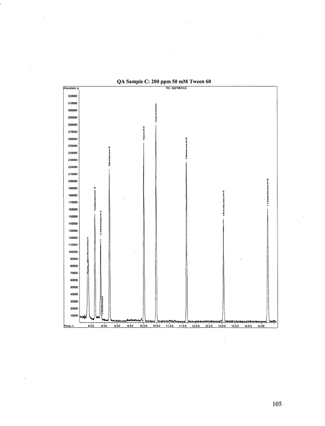
ppm PCE with 5% Dowfax, and Sample C at 200 ppm PCE with 50 mM Tween 60. These
data compare the measured concentration of PCE to the expected or theoretical
concentration in each sample aliquot using GC/MS. The actual concentrations were
acceptably close to the theoretical concentrations. Specifically, the theoretical PCE
concentration for Sample A was within 6% of the GC/MS measured PCE concentration.
Further inspection of the data table reveals Sample B was within 3%, and Sample C within
5.5%. These GC/MS results demonstrate that the PCE concentrations used in the
experimental treatments meet the project objectives.
The QA/QC data included in Appendices E and F demonstrate that these
instruments operated within the project quality objectives, and that the experimental data
generated from these instruments are of acceptable quality.
10
image:
2.2.5 Density Measurements
Density was calculated from volume and mass measurements. The volume was
determined by inspection of a graduated cylinder at room temperature (@ 25°C). Mass was
measured using a Sartorius scale Model Number 3876 MP8-2, which was calibrated prior
to each use.
2.2.6 GC/MS Volatile Compound Analyses
All samples were stored at 0°C and analyzed within 14 days of preparation, if
possible. Samples were introduced by using Method 5035B, Purge-and-Trap, as per SW-
846 (USEPA, 1996; USEPA, 1996), and analyzed by GC/MS following the procedures in
EPA SW-846 Method 8260B, Volatile Organic Compounds by Gas Chromatography/Mass
Spectrometry (GC/MS): Capillary Technique (USEPA, 1996; USEPA, 2004). The
instrument was calibrated using internal standards for PCE and the applicable surrogate,
without regard to the other compounds listed in the method. Quality Assurance/Quality
Control (QA/QC) followed the guidelines in the Quality Assurance Project Plan (QAPP)
(Werkema, 2006).
3.0 Results and Analysis
3.1 Quality Assurance / Quality Control
All data were collected using the SOPs specific to each instrument. The data and the SOPs
are included in the appendices. Appendix A summarizes the QA/QC protocols for the data
and references the QAPP for this project (Werkema, 2006). Appendix E includes the data
for the electrochemical measurement QA/QC. These analyses consist of: the individual
instrument calibrations per analytical date; and the initial calibrations, repeatability, and
potential instrument drift calculations. Furthermore, Appendix E indicates if any corrective
action was taken or if ongoing calibration check measurements were out of specifications.
To evaluate the quality of the data, comparability is used as a qualitative parameter
expressing the confidence with which one data set can be compared with another (Stanely
and Verner, 1985). The data comparability of the PCE concentration was determined
through external analysis PCE by GC/MS analysis. Appendix F includes the data for three
select QA/QC samples: Sample A at 50 ppm PCE with 4% Tween 80, Sample B at 100
ppm PCE with 5% Dowfax, and Sample C at 200 ppm PCE with 50 mM Tween 60. These
data compare the measured concentration of PCE to the expected or theoretical
concentration in each sample aliquot using GC/MS. The actual concentrations were
acceptably close to the theoretical concentrations. Specifically, the theoretical PCE
concentration for Sample A was within 6% of the GC/MS measured PCE concentration.
Further inspection of the data table reveals Sample B was within 3%, and Sample C within
5.5%. These GC/MS results demonstrate that the PCE concentrations used in the
experimental treatments meet the project objectives.
The QA/QC data included in Appendices E and F demonstrate that these
instruments operated within the project quality objectives, and that the experimental data
generated from these instruments are of acceptable quality.
10
image:
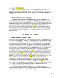 3.2 Temperature Response
The temperature response was first investigated for the possible requirement of a
transform of the data. The temperature response ranges from 15.9 to 21.7 with a
maximum-to-minimum ratio of approximately 1.36. Generally, a ratio greater than 10
indicates that a transform is required, and the power transform has little effect for ratios
less than three (Stat-Ease, 2006). Because the temperature response ratio is low, no
transform was performed. Furthermore, the Box-Cox (Box and Cox, 1964) plot shown in
Figure 1 does not indicate a recommendation for a power law transform.
Lambda
Current = 1
Best = 2.3
Low C.I. = 0.31
High C.I. = 4.32
Recommend transform:
None
(Lambda = 1)
5.79-
5.76-
5.73-
5.70-
5.67-
Figure 1. Temperature Response Box-Cox Plot
Box and Cox (1964) analyzed transforms of data to alleviate the confining assumption of
data normality and homoscedasticity. That is, data analysis typically assumes that
observations (yO are independently normally distributed with constant variance over the
design space for constructing a linear model and a defined set of parameters. The Box-Cox
plot is a tool used by the software, Design Expert (Stat-Ease, 2006) to determine the most
appropriate power transformation applicable to the response data to account for these
assumptions. As described by Stat-Ease, Inc. (2006), response data transforms can be
described by the power function, a = fnyi"}, where o is the standard deviation, u is the
mean, and a is the power. Lambda (A.) is 1- a and is used as the A, power transform scale
such that if the standard deviation associated with an observation is proportional to the
mean raised to a power, then transforming the observation by the A, power results in a scale
that stabilizes the variance. The lowest point in a Box-Cox plot determines the value of X
which results in the minimum residual sum-of-squares in the transformed model. A
maximum-to-minimum ratio greater than three indicates that the potential for improvement
11
image:
3.2 Temperature Response
The temperature response was first investigated for the possible requirement of a
transform of the data. The temperature response ranges from 15.9 to 21.7 with a
maximum-to-minimum ratio of approximately 1.36. Generally, a ratio greater than 10
indicates that a transform is required, and the power transform has little effect for ratios
less than three (Stat-Ease, 2006). Because the temperature response ratio is low, no
transform was performed. Furthermore, the Box-Cox (Box and Cox, 1964) plot shown in
Figure 1 does not indicate a recommendation for a power law transform.
Lambda
Current = 1
Best = 2.3
Low C.I. = 0.31
High C.I. = 4.32
Recommend transform:
None
(Lambda = 1)
5.79-
5.76-
5.73-
5.70-
5.67-
Figure 1. Temperature Response Box-Cox Plot
Box and Cox (1964) analyzed transforms of data to alleviate the confining assumption of
data normality and homoscedasticity. That is, data analysis typically assumes that
observations (yO are independently normally distributed with constant variance over the
design space for constructing a linear model and a defined set of parameters. The Box-Cox
plot is a tool used by the software, Design Expert (Stat-Ease, 2006) to determine the most
appropriate power transformation applicable to the response data to account for these
assumptions. As described by Stat-Ease, Inc. (2006), response data transforms can be
described by the power function, a = fnyi"}, where o is the standard deviation, u is the
mean, and a is the power. Lambda (A.) is 1- a and is used as the A, power transform scale
such that if the standard deviation associated with an observation is proportional to the
mean raised to a power, then transforming the observation by the A, power results in a scale
that stabilizes the variance. The lowest point in a Box-Cox plot determines the value of X
which results in the minimum residual sum-of-squares in the transformed model. A
maximum-to-minimum ratio greater than three indicates that the potential for improvement
11
image:
 is greatest when using the power transform (Stat-Ease, 2006). The Box-Cox plot is used in
the analysis of all the responses.
The fit summary for the temperature response was next examined. These data are
shown in Table III, Temperature Response Fit Summary.
Table III: Temperature Response Fit Summary
Response: Temp Transform:
Sequential Model Sum of Squares [Type I]
None
Source
Mean vs. Total
Linear vs. Mean
2FI vs. Linear
Quadratic vs. 2FI
Cubic vs.
Quadratic
Residual
Total
Sum-of-
Squares
87054.7
32.69
28.02
1.02
33.08
228.16
87377.67
df
1
12
29
1
30
167
240
Mean
Square
87054.7
2.72
0.97
1.02
1.1
1.37
364.07
F
Value
2.13
0.73
0.77
0.81
p-value
Prob > F
0.016
0.8426
0.3808
0.7511
Suggested
Suggested
Lack-of-Fit Tests
Source
Linear
2FI
Quadratic
Cubic
Pure Error
Sum-of-
Squares
181.19
153.17
152.15
119.07
109.09
df
137
108
107
77
90
Mean
Square
1.32
1.42
1.42
1.55
1.21
F
Value'
1.09
1.17
1.17
1.28
p-value
Prob > F
0.3304
0.2213
0.2179
0.1327
Suggested
Model Summary Statistics
Source
Std. Dev.
Adjusted Predicted
R2 R2
PRESS
Linear
2FI
Quadratic
Cubic
1.13
1.15
1.15
1.17
0.1012
0.188
0.1912
0.2936
0.0537
0.0198
0.0187
-0.011
-0.0045
-0.1879
-0.1951
-0.4735
324.42
383.66
386
475.91
Suggested
Inspection of the sequential model sum-of-squares is used to select the highest order
polynomial where the additional terms are significant and the model main factors are not
aliased. This suggests the mean or linear (i.e. first order main effects factors) model. The
lack-of-fit F-test suggests the linear model, as not having a significant lack-of-fit (i.e., it is
desirable for the model to have an insignificant lack-of-fit). The model summary statistics
allow inspection of the Adjusted R2 and the Predicted R2 (see Appendix H for definition).
Better models maximize both of these values; however, these results show very low values
12
image:
is greatest when using the power transform (Stat-Ease, 2006). The Box-Cox plot is used in
the analysis of all the responses.
The fit summary for the temperature response was next examined. These data are
shown in Table III, Temperature Response Fit Summary.
Table III: Temperature Response Fit Summary
Response: Temp Transform:
Sequential Model Sum of Squares [Type I]
None
Source
Mean vs. Total
Linear vs. Mean
2FI vs. Linear
Quadratic vs. 2FI
Cubic vs.
Quadratic
Residual
Total
Sum-of-
Squares
87054.7
32.69
28.02
1.02
33.08
228.16
87377.67
df
1
12
29
1
30
167
240
Mean
Square
87054.7
2.72
0.97
1.02
1.1
1.37
364.07
F
Value
2.13
0.73
0.77
0.81
p-value
Prob > F
0.016
0.8426
0.3808
0.7511
Suggested
Suggested
Lack-of-Fit Tests
Source
Linear
2FI
Quadratic
Cubic
Pure Error
Sum-of-
Squares
181.19
153.17
152.15
119.07
109.09
df
137
108
107
77
90
Mean
Square
1.32
1.42
1.42
1.55
1.21
F
Value'
1.09
1.17
1.17
1.28
p-value
Prob > F
0.3304
0.2213
0.2179
0.1327
Suggested
Model Summary Statistics
Source
Std. Dev.
Adjusted Predicted
R2 R2
PRESS
Linear
2FI
Quadratic
Cubic
1.13
1.15
1.15
1.17
0.1012
0.188
0.1912
0.2936
0.0537
0.0198
0.0187
-0.011
-0.0045
-0.1879
-0.1951
-0.4735
324.42
383.66
386
475.91
Suggested
Inspection of the sequential model sum-of-squares is used to select the highest order
polynomial where the additional terms are significant and the model main factors are not
aliased. This suggests the mean or linear (i.e. first order main effects factors) model. The
lack-of-fit F-test suggests the linear model, as not having a significant lack-of-fit (i.e., it is
desirable for the model to have an insignificant lack-of-fit). The model summary statistics
allow inspection of the Adjusted R2 and the Predicted R2 (see Appendix H for definition).
Better models maximize both of these values; however, these results show very low values
12
image:
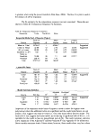 and a negative Predicted-R2. A negative Pred-R2 may suggest the mean is a better
predictor than the model. Because the negative Pred-R2 is very small for the linear model
an analysis of variance (ANOVA) was performed using the linear model. The regression
algorithm for the ANOVA used is stepwise regression. Stepwise regression is a
modification of forward regression in that along the step of the regression a reexamination
of the factors incorporated into the model from the previous step is completed (Kleinbaum
et al., 1998). For instance, a factor that entered at an earlier stage may become extra at a
later stage because of its relationship with the additional factors subsequently added to the
model. To evaluate this possibility, the stepwise regression procedure makes a partial F-
test at each step for each factor currently in the model. The factor with the smallest non-
significant partial F-statistic (if such a variable exists) is removed. The model is then
refitted with the remaining factors, and the partial F-tests are obtained, evaluated, and so
on, until no more factors can be entered or removed (Kleinbaum et al., 1998). In Design
Expert (Stat-Ease, 2006) the Alpha to enter and Alpha to exit is this partial F-statistic flag
and are each set to 1.00 by default. The stepwise regression technique requires the value of
Alpha-In to be less than or equal to the Alpha-Out value. Using the default value, the
overall model contains terms at the 0.05 level of significance. This stepwise regression
process effectively reduces the complexity of the model and provides a model with only the
F-test significant factors, hi this report, the ANOVA for all responses are completed with
stepwise regression with the default Alpha values. The results from this procedure for the
temperature response are shown in Table IV, Temperature Response ANOVA. The model
F-value of 2.19 implies the model is significant and there is a 1.58% chance that a model F-
value this large could occur due to residual uncertainty or variance (i.e. noise). Values of
Prob>F less than 0.05 are used to indicate that the model factors are significant. The
ANOVA table indicates that the factor terms B-Dye type and C-Surfactant type are
significant model factors. Non-significant factors, those with Prob>F values greater than
0.1000, were not included in the model through the stepwise regression algorithm. The
Lack of Fit F-value of 1.09 suggests that the lack-of-fit is not significant relative to the pure
error (i.e. purely experimental uncertainty). That is, there is a 32.50% chance that a lack-
of-fit F-value this large could occur due to purely experimental uncertainty. The Pred-R2 is
within the desirable range of 0.2 (Stat-Ease, 2006) less than the Adj-R2; however, the R2
value is quite low and the Pred-R is negative, which again implies that the overall mean is
a better predictor of the temperature response than the linear model. This confirms the
Temperature Response Summary in Table III. The adequate precision of the model is
5.680 and is greater than four (Anderson and Whitcomb, 2005). Adequate precision is a
measure of the range in the predicted response relative to its associated error; in other
words, a signal-to-noise ratio. It compares the range of the predicted values at the design
points to the average prediction error. Ratios greater than four indicate adequate model
discrimination.
13
image:
and a negative Predicted-R2. A negative Pred-R2 may suggest the mean is a better
predictor than the model. Because the negative Pred-R2 is very small for the linear model
an analysis of variance (ANOVA) was performed using the linear model. The regression
algorithm for the ANOVA used is stepwise regression. Stepwise regression is a
modification of forward regression in that along the step of the regression a reexamination
of the factors incorporated into the model from the previous step is completed (Kleinbaum
et al., 1998). For instance, a factor that entered at an earlier stage may become extra at a
later stage because of its relationship with the additional factors subsequently added to the
model. To evaluate this possibility, the stepwise regression procedure makes a partial F-
test at each step for each factor currently in the model. The factor with the smallest non-
significant partial F-statistic (if such a variable exists) is removed. The model is then
refitted with the remaining factors, and the partial F-tests are obtained, evaluated, and so
on, until no more factors can be entered or removed (Kleinbaum et al., 1998). In Design
Expert (Stat-Ease, 2006) the Alpha to enter and Alpha to exit is this partial F-statistic flag
and are each set to 1.00 by default. The stepwise regression technique requires the value of
Alpha-In to be less than or equal to the Alpha-Out value. Using the default value, the
overall model contains terms at the 0.05 level of significance. This stepwise regression
process effectively reduces the complexity of the model and provides a model with only the
F-test significant factors, hi this report, the ANOVA for all responses are completed with
stepwise regression with the default Alpha values. The results from this procedure for the
temperature response are shown in Table IV, Temperature Response ANOVA. The model
F-value of 2.19 implies the model is significant and there is a 1.58% chance that a model F-
value this large could occur due to residual uncertainty or variance (i.e. noise). Values of
Prob>F less than 0.05 are used to indicate that the model factors are significant. The
ANOVA table indicates that the factor terms B-Dye type and C-Surfactant type are
significant model factors. Non-significant factors, those with Prob>F values greater than
0.1000, were not included in the model through the stepwise regression algorithm. The
Lack of Fit F-value of 1.09 suggests that the lack-of-fit is not significant relative to the pure
error (i.e. purely experimental uncertainty). That is, there is a 32.50% chance that a lack-
of-fit F-value this large could occur due to purely experimental uncertainty. The Pred-R2 is
within the desirable range of 0.2 (Stat-Ease, 2006) less than the Adj-R2; however, the R2
value is quite low and the Pred-R is negative, which again implies that the overall mean is
a better predictor of the temperature response than the linear model. This confirms the
Temperature Response Summary in Table III. The adequate precision of the model is
5.680 and is greater than four (Anderson and Whitcomb, 2005). Adequate precision is a
measure of the range in the predicted response relative to its associated error; in other
words, a signal-to-noise ratio. It compares the range of the predicted values at the design
points to the average prediction error. Ratios greater than four indicate adequate model
discrimination.
13
image:
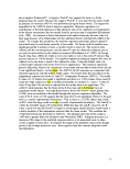 Table. IV: Temperature Response ANOVA
Response: Temperature
Stepwise Regression with Alpha to Enter = 0.100, Alpha to Exit = 0.100
Forced Terms: Intercept
Added
B-Dye
C-Surfactant
F Value
3.07
1.97
p-value Prob > F
0.0482
0.0438
R2
0.0253
0.0955
MSE
1.33
1.28
ANOVA for Response Surface Reduced Linear Model
Analysis of Variance Table [Classical Sum-of-Squares - Type II]
Source
Model
B-Dye
C-Surfactant
Residual
Lack-of-Fit
Purely
experimental
uncertainty
Cor Total
Sum-of-
Squares
30.86
8.16
22.7
292.12
183.03
109.09
322.97
df
11
2
9
228
138
90
239
Mean
Square
2.81
4.08
2.52
1.28
1.33
1.21
F Value
2.19
3.18
1.97
1.09
p-value
Prob > F
0.0158
0.0432
0.044
0.325
significant
not significant
Std. Dev.
Mean
C.V. %
PRESS
1.13
19.05
5.94
323.68
R'
AdjR2
Pred R2
Adeq Precision
0.0955
0.0519
-0.0022
5.68
Next, the ANOVA assumptions were verified by inspecting the Residual Analysis
and Diagnostics plots. Figure 2 includes the Temperature Response Diagnostic plots.
First, the Normal Plot of the Internally Studentized Residuals (Fig. 2 A) shows a linear or
normal relationship; this normality assumption is valid. Figure 2B shows the Internally
14
image:
Table. IV: Temperature Response ANOVA
Response: Temperature
Stepwise Regression with Alpha to Enter = 0.100, Alpha to Exit = 0.100
Forced Terms: Intercept
Added
B-Dye
C-Surfactant
F Value
3.07
1.97
p-value Prob > F
0.0482
0.0438
R2
0.0253
0.0955
MSE
1.33
1.28
ANOVA for Response Surface Reduced Linear Model
Analysis of Variance Table [Classical Sum-of-Squares - Type II]
Source
Model
B-Dye
C-Surfactant
Residual
Lack-of-Fit
Purely
experimental
uncertainty
Cor Total
Sum-of-
Squares
30.86
8.16
22.7
292.12
183.03
109.09
322.97
df
11
2
9
228
138
90
239
Mean
Square
2.81
4.08
2.52
1.28
1.33
1.21
F Value
2.19
3.18
1.97
1.09
p-value
Prob > F
0.0158
0.0432
0.044
0.325
significant
not significant
Std. Dev.
Mean
C.V. %
PRESS
1.13
19.05
5.94
323.68
R'
AdjR2
Pred R2
Adeq Precision
0.0955
0.0519
-0.0022
5.68
Next, the ANOVA assumptions were verified by inspecting the Residual Analysis
and Diagnostics plots. Figure 2 includes the Temperature Response Diagnostic plots.
First, the Normal Plot of the Internally Studentized Residuals (Fig. 2 A) shows a linear or
normal relationship; this normality assumption is valid. Figure 2B shows the Internally
14
image:
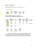 B)
1
-1.75 -0*8 0.79
Internally Studentized Resduals
I
• 15.9
Temp:
~T
I
18.83
I
1961
Predicted
C)
D)
1735-
21.7
35 89 103 137 171 205 239
Run Number
18.80
Actual
2025
T
21.70
Figure 2. Temperature Response Diagnostics; A) Normal Plot of Internally Studentized Residuals, B)
Internally Studentized Residuals vs. Predicted, C) Internally Studentized Residuals vs. Run, and D) Predicted
vs. Actual
Studentized Residuals vs. Predicted plot. This plot shows random scatter, not a megaphone
shape or any general shape, which is desirable in that it indicates that there are no trends in
the residuals. The plot of the Internally Studentized Residuals vs. Run (Fig. 2C) also
displays a favorable random pattern and indicates no pattern in the relationship between
residuals and run number. The Predicted vs. Actual plot (Fig. 2D) supports the observation
of the negative Pred-R , where the indication is that the mean may be a better predictor
than the model. This plot shows an even grouping of points on either side of the 45° line
and clustered about the average predicted value of 19.05, as in the ANOVA output, hi
order to support the model as a good predictor, points on this plot should be relatively
randomly distributed about the 45° line. Figure 3 shows the Internally Studentized
15
image:
B)
1
-1.75 -0*8 0.79
Internally Studentized Resduals
I
• 15.9
Temp:
~T
I
18.83
I
1961
Predicted
C)
D)
1735-
21.7
35 89 103 137 171 205 239
Run Number
18.80
Actual
2025
T
21.70
Figure 2. Temperature Response Diagnostics; A) Normal Plot of Internally Studentized Residuals, B)
Internally Studentized Residuals vs. Predicted, C) Internally Studentized Residuals vs. Run, and D) Predicted
vs. Actual
Studentized Residuals vs. Predicted plot. This plot shows random scatter, not a megaphone
shape or any general shape, which is desirable in that it indicates that there are no trends in
the residuals. The plot of the Internally Studentized Residuals vs. Run (Fig. 2C) also
displays a favorable random pattern and indicates no pattern in the relationship between
residuals and run number. The Predicted vs. Actual plot (Fig. 2D) supports the observation
of the negative Pred-R , where the indication is that the mean may be a better predictor
than the model. This plot shows an even grouping of points on either side of the 45° line
and clustered about the average predicted value of 19.05, as in the ANOVA output, hi
order to support the model as a good predictor, points on this plot should be relatively
randomly distributed about the 45° line. Figure 3 shows the Internally Studentized
15
image:
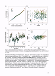 A)
I
• 15.9
Temp:
149 -
-152 -
i :
,
I
2
!
s
• 2
|
i
I 3
m
m
]
1 '
:
i
B)
33 67 100 133 1«7 200
PCEconc
121 7
15.9
Temp:
Dye
C)
I
115.9
Temp:
1 8 J_L
•«
i
•
« • m
. : , i i i .
• 1 ' : :* i ! I
• ' •
10
Surfactant
Figure 3. Temperature Response Internally Studentized
Residuals vs. Factors; A) Internally Studentized Residuals
vs. PCE concentration, B) Internally Studentized Residuals
vs. Dye, C) Residuals vs. Surfactant
Residuals vs. the three factors: PCE
concentration (Fig. 3A), Dye type (Fig.
3B), and Surfactant type (Fig. 3C).
These plots show an even split about
the zero-line at either end of the range
of each factor with no obvious main
effect or grouping of points biasing the
scatter. This random scatter is
acceptable for the support of ANOVA
assumptions.
Influence plots investigate
outliers and include statistics which
examine each run to see how it affects
the model fit. Results from the
temperature response experiments were
analyzed for the presence of outliers.
An outlier is any rare or unusual
observation that appears at one of the
extremes of the data range (Kleinbaum
et al., 1998). Figure 4 includes the
Influence Plots. The Externally
Studentized or outlier-t value Residuals
(Fig. 4A) show that all of the values are
within the 95% confidence limits,
which are shown as the red horizontal
lines. The Difference in Fits (DFFITS)
vs. Run plot (Fig. 4B) also reveals no
overly influential runs as all points are
plotted within the bounds shown.
Another useful tool to
investigate for outliers or influential
runs is Cook's distance. Cook's
distance is a measure of how much the
estimated parameters would change if
that particular experimental run were
omitted from the analysis (Anderson et
al., 2006; Kleinbaum et al., 1998;
Montgomery, 1997). It is roughly a
combination of the leverage and the
outlier. It is used to help identify
individual runs that may be outliers.
The values generated are relative
(Anderson and Whitcomb, 2005;
Anderson et al., 2006; Kleinbaum et al.,
1998) in that if a value is much higher
than the others it might indicate an
16
image:
A)
I
• 15.9
Temp:
149 -
-152 -
i :
,
I
2
!
s
• 2
|
i
I 3
m
m
]
1 '
:
i
B)
33 67 100 133 1«7 200
PCEconc
121 7
15.9
Temp:
Dye
C)
I
115.9
Temp:
1 8 J_L
•«
i
•
« • m
. : , i i i .
• 1 ' : :* i ! I
• ' •
10
Surfactant
Figure 3. Temperature Response Internally Studentized
Residuals vs. Factors; A) Internally Studentized Residuals
vs. PCE concentration, B) Internally Studentized Residuals
vs. Dye, C) Residuals vs. Surfactant
Residuals vs. the three factors: PCE
concentration (Fig. 3A), Dye type (Fig.
3B), and Surfactant type (Fig. 3C).
These plots show an even split about
the zero-line at either end of the range
of each factor with no obvious main
effect or grouping of points biasing the
scatter. This random scatter is
acceptable for the support of ANOVA
assumptions.
Influence plots investigate
outliers and include statistics which
examine each run to see how it affects
the model fit. Results from the
temperature response experiments were
analyzed for the presence of outliers.
An outlier is any rare or unusual
observation that appears at one of the
extremes of the data range (Kleinbaum
et al., 1998). Figure 4 includes the
Influence Plots. The Externally
Studentized or outlier-t value Residuals
(Fig. 4A) show that all of the values are
within the 95% confidence limits,
which are shown as the red horizontal
lines. The Difference in Fits (DFFITS)
vs. Run plot (Fig. 4B) also reveals no
overly influential runs as all points are
plotted within the bounds shown.
Another useful tool to
investigate for outliers or influential
runs is Cook's distance. Cook's
distance is a measure of how much the
estimated parameters would change if
that particular experimental run were
omitted from the analysis (Anderson et
al., 2006; Kleinbaum et al., 1998;
Montgomery, 1997). It is roughly a
combination of the leverage and the
outlier. It is used to help identify
individual runs that may be outliers.
The values generated are relative
(Anderson and Whitcomb, 2005;
Anderson et al., 2006; Kleinbaum et al.,
1998) in that if a value is much higher
than the others it might indicate an
16
image:
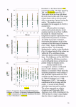 outlier. Relatively large values are associated with cases with high leverage and large
studentized residuals. Large values could be caused by recording errors, an incorrect
model, or a design point far from the remaining cases and should be investigated. "Large"
is sometimes defined as a point that is two-to-three times larger than the other points. For
further details, definitions, and the calculation of Cook's distance, refer to Appendix G.
Figure 4, Temperature Response Influence Plots, includes the Cook's Distance plot for the
Temperature response (Fig. 4C), which also shows no outliers present. Finally, the
leverage of run was investigated. Leverage is the potential for a design point to influence
the fit of the model coefficients. Large values, and especially values at or near one, should
be avoided. The Leverage vs. Run plot (Fig. 4D) does not reveal any values which exhibit
any undue influence on the model parameters. Overall, the influence plots reveal that no
runs have overly influenced the Temperature Response and no outliers are present.
A)
-3.77 -
no
rf
f /
I
115.9
Temp:
B)
1 35 69 103 137 171 205 239
Run Number
1 35 69 103 137 171 205 239
C)
„ 050 -
oxx>
I
•15.9
Temp:
D)
121.7
15.9
Temp:
1 35 «9 103 137 171 205 239
Run Number
1 35 69 103 137 171 205 239
ftjn Number
Figure 4. Temperature Response Influence Plots A) Externally Studentized Residuals, B) DFFITS vs. Run,
C) Cook's Distance, D) Leverage vs. Run
17
image:
outlier. Relatively large values are associated with cases with high leverage and large
studentized residuals. Large values could be caused by recording errors, an incorrect
model, or a design point far from the remaining cases and should be investigated. "Large"
is sometimes defined as a point that is two-to-three times larger than the other points. For
further details, definitions, and the calculation of Cook's distance, refer to Appendix G.
Figure 4, Temperature Response Influence Plots, includes the Cook's Distance plot for the
Temperature response (Fig. 4C), which also shows no outliers present. Finally, the
leverage of run was investigated. Leverage is the potential for a design point to influence
the fit of the model coefficients. Large values, and especially values at or near one, should
be avoided. The Leverage vs. Run plot (Fig. 4D) does not reveal any values which exhibit
any undue influence on the model parameters. Overall, the influence plots reveal that no
runs have overly influenced the Temperature Response and no outliers are present.
A)
-3.77 -
no
rf
f /
I
115.9
Temp:
B)
1 35 69 103 137 171 205 239
Run Number
1 35 69 103 137 171 205 239
C)
„ 050 -
oxx>
I
•15.9
Temp:
D)
121.7
15.9
Temp:
1 35 «9 103 137 171 205 239
Run Number
1 35 69 103 137 171 205 239
ftjn Number
Figure 4. Temperature Response Influence Plots A) Externally Studentized Residuals, B) DFFITS vs. Run,
C) Cook's Distance, D) Leverage vs. Run
17
image:
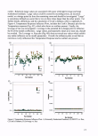 Because the stepwise regression ANOVA found dye and surfactant type significant
factors for the linear model temperature response, these results are shown in a matrix in
Figure 5, Temperature Response: Dye vs. Surfactant.
c
-«
No Surfactant —
5%Dowfax8390—
05%Dowfex8390-
0.1%SteolCS-330 —
0.025% SeolCS-330 —
8%AMA-80-I —
05%AMA-80-I —
50mMTween60 —
4%Tween80 + 10%BOH —
4%Tween80 —
19.5253
19.0842
m0217
19.2717
19.3425
18.7006
19.4967
ia5133
19.2342
iai467
I
none
19.1606 19.6058
ia7392 iai642
ia67B7 iaiQ17
ia9267 ia3517
ia9975 19.4225
ia3558 larsoe
19.1517 19.5767
iai6B3 ia5933
ia8892 19.3142
ia8017 19.2267
I I
BB. Oil-Red-O
Dye
Figure 5. Temperature Response: Dye vs. Surfactant at 100 ppm PCE
Inspection of this model matrix reveals a small range of values from 19.6058 to 18.1683, a
mean of 19.05, and a standard deviation of 1.13. The temperature probes used have a
resolution and accuracy of 0.1 °C resolution, ± 0.3 °C for the Denver Instrument
Electrochemistry Meter and 0.1 °C resolution, ± 0.1° C for the Accumet® Model AR 60
Meter. Since the temperature data used in the model development was an average from
these meters, the standard deviation of the model response is within the resolution and
accuracy of the meters. In summary, due to the low R2 of 0.0955, and the Pred-R2 of
-0.0022, the mean of the temperature response is likely a better predictor than the linear
model. However, since the Adeq Precision measures the signal-to-noise rate, and was
5.680, it is acceptable to use the model for predictive purposes. Therefore, the final
equation in terms of coded factors is given below.
18
image:
Because the stepwise regression ANOVA found dye and surfactant type significant
factors for the linear model temperature response, these results are shown in a matrix in
Figure 5, Temperature Response: Dye vs. Surfactant.
c
-«
No Surfactant —
5%Dowfax8390—
05%Dowfex8390-
0.1%SteolCS-330 —
0.025% SeolCS-330 —
8%AMA-80-I —
05%AMA-80-I —
50mMTween60 —
4%Tween80 + 10%BOH —
4%Tween80 —
19.5253
19.0842
m0217
19.2717
19.3425
18.7006
19.4967
ia5133
19.2342
iai467
I
none
19.1606 19.6058
ia7392 iai642
ia67B7 iaiQ17
ia9267 ia3517
ia9975 19.4225
ia3558 larsoe
19.1517 19.5767
iai6B3 ia5933
ia8892 19.3142
ia8017 19.2267
I I
BB. Oil-Red-O
Dye
Figure 5. Temperature Response: Dye vs. Surfactant at 100 ppm PCE
Inspection of this model matrix reveals a small range of values from 19.6058 to 18.1683, a
mean of 19.05, and a standard deviation of 1.13. The temperature probes used have a
resolution and accuracy of 0.1 °C resolution, ± 0.3 °C for the Denver Instrument
Electrochemistry Meter and 0.1 °C resolution, ± 0.1° C for the Accumet® Model AR 60
Meter. Since the temperature data used in the model development was an average from
these meters, the standard deviation of the model response is within the resolution and
accuracy of the meters. In summary, due to the low R2 of 0.0955, and the Pred-R2 of
-0.0022, the mean of the temperature response is likely a better predictor than the linear
model. However, since the Adeq Precision measures the signal-to-noise rate, and was
5.680, it is acceptable to use the model for predictive purposes. Therefore, the final
equation in terms of coded factors is given below.
18
image:
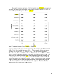 Temp =
+19.05
+0.088 *B[1]
-0.26 * B[2]
+0.013 *C[1]
+0.10*C[2]
-0.62 * C[3]
+0.36 * C[4]
-0.43 * C[5]
+0.21 * C[6]
+0.14*C[7]
-0.11 *C[8]
-0.050 * C[9]
With the following error analysis:
Term
Intercept
B[1]
B[2]
C[1]
era
C[3]
C[4]
C[5]
C[6]
cm
C[8]
C[9]
Coefficient
Estimate
19.04542
0.088333
-0.25667
0.012917
0.100417
-0.62042
0.362917
-0.43292
0.20875
0.137917
-0.11208
-0.04958
df
1
1
1
1
1
1
1
1
1
1
1
1
Standard
Error
0.073064
0.103329
0.103329
0.219193
0.219193
0.219193
0.219193
0.219193
0.219193
0.219193
0.219193
0.219193
95% Cl
Low
18.90145
-0.11527
-0.46027
-0.41899
-0.33149
-1.05232
-0.06899
-0.86482
-0.22315
-0.29399
-0.54399
-0.48149
95% Cl
High
19.18938
0.291935
-0.05307
0.444821
0.532321
-0.18851
0.794821
-0.00101
0.640654
0.569821
0.319821
0.382321
19
image:
Temp =
+19.05
+0.088 *B[1]
-0.26 * B[2]
+0.013 *C[1]
+0.10*C[2]
-0.62 * C[3]
+0.36 * C[4]
-0.43 * C[5]
+0.21 * C[6]
+0.14*C[7]
-0.11 *C[8]
-0.050 * C[9]
With the following error analysis:
Term
Intercept
B[1]
B[2]
C[1]
era
C[3]
C[4]
C[5]
C[6]
cm
C[8]
C[9]
Coefficient
Estimate
19.04542
0.088333
-0.25667
0.012917
0.100417
-0.62042
0.362917
-0.43292
0.20875
0.137917
-0.11208
-0.04958
df
1
1
1
1
1
1
1
1
1
1
1
1
Standard
Error
0.073064
0.103329
0.103329
0.219193
0.219193
0.219193
0.219193
0.219193
0.219193
0.219193
0.219193
0.219193
95% Cl
Low
18.90145
-0.11527
-0.46027
-0.41899
-0.33149
-1.05232
-0.06899
-0.86482
-0.22315
-0.29399
-0.54399
-0.48149
95% Cl
High
19.18938
0.291935
-0.05307
0.444821
0.532321
-0.18851
0.794821
-0.00101
0.640654
0.569821
0.319821
0.382321
19
image:
 3.3 pH Response
The pH response ranged from 4.32 to 7.96 with a maximum-to-minimum ratio of
1.84259; therefore, no transformation was required. The Box-Cox plot (Fig. 6) also
confirms that no transformation is recommended, with lambda = 1 recommended.
3.85-
2.73 —
Figure 6: pH Response Box-Cox Plot
20
image:
3.3 pH Response
The pH response ranged from 4.32 to 7.96 with a maximum-to-minimum ratio of
1.84259; therefore, no transformation was required. The Box-Cox plot (Fig. 6) also
confirms that no transformation is recommended, with lambda = 1 recommended.
3.85-
2.73 —
Figure 6: pH Response Box-Cox Plot
20
image:
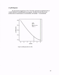 The pH response fit summary is shown in Table V. The sequential model sum-of-squares
suggests a linear model with a Prob>F of O.0001 and the model is not aliased.
Table V: pH Response Fit Summary
Response: pH Transform:
Sequential Model Sum of Squares [Type I]
None
Source
Mean vs. Total
Linear vs. Mean
2FI vs. Linear
Quadratic vs. 2FI
Cubic vs.
Quadratic
Residual
Total
Sum-of-
Squares
8508.39
88.72
2.25
0.046
2.51
13.41
8615.33
df
1
12
29
1
30
167
240
Mean
Square
8508.39
7.39
0.078
0.046
0.084
0.08
35.9
F
Value
92.1
0.96
0.56
1.04
p-value
Prob > F
< 0.0001
0.526
0.4534
0.4157
Suggested
Lack-of-Fit Tests
Source
Linear
2FI
Quadratic
Cubic
Pure Experimental
Uncertainty
Sum-of-
Squares
11.69
9.43
9.39
6.88
6.54
df
137
108
107
77
90
Mean
Square
0.085
0.087
0.088
0.089
0.073
F
Value
1.17
1.2
1.21
1.23
p-value
Prob > F
0.2068
0.1833
0.1779
0.172
Suggested
Model Summary Statistics
Source
Linear
2FI
Quadratic
Cubic
Std. Dev.
0.28
0.28
0.28
0.28
R2
0.8296
0.8507
0.8511
0.8746 '
Adjusted
R2
0.8206
0.8197
0.8193
0.8205
Predicted
R2
0.8097
0.7831
0.7814
0.743
PRESS
20.36
23.2
23.38
27.49
Suggested
This is also supported by the lack-of-fit test with Prob>F of 0.2068, again it is desirable to
have an insignificant lack-of-fit. The model summary statistics also show that the highest
R2 of 0.8296 for the linear model, and the Adj-R2 of 0.8206 and Pred-R2 of 0.8097 are
within the desirable ±0.2 range of each other.
21
image:
The pH response fit summary is shown in Table V. The sequential model sum-of-squares
suggests a linear model with a Prob>F of O.0001 and the model is not aliased.
Table V: pH Response Fit Summary
Response: pH Transform:
Sequential Model Sum of Squares [Type I]
None
Source
Mean vs. Total
Linear vs. Mean
2FI vs. Linear
Quadratic vs. 2FI
Cubic vs.
Quadratic
Residual
Total
Sum-of-
Squares
8508.39
88.72
2.25
0.046
2.51
13.41
8615.33
df
1
12
29
1
30
167
240
Mean
Square
8508.39
7.39
0.078
0.046
0.084
0.08
35.9
F
Value
92.1
0.96
0.56
1.04
p-value
Prob > F
< 0.0001
0.526
0.4534
0.4157
Suggested
Lack-of-Fit Tests
Source
Linear
2FI
Quadratic
Cubic
Pure Experimental
Uncertainty
Sum-of-
Squares
11.69
9.43
9.39
6.88
6.54
df
137
108
107
77
90
Mean
Square
0.085
0.087
0.088
0.089
0.073
F
Value
1.17
1.2
1.21
1.23
p-value
Prob > F
0.2068
0.1833
0.1779
0.172
Suggested
Model Summary Statistics
Source
Linear
2FI
Quadratic
Cubic
Std. Dev.
0.28
0.28
0.28
0.28
R2
0.8296
0.8507
0.8511
0.8746 '
Adjusted
R2
0.8206
0.8197
0.8193
0.8205
Predicted
R2
0.8097
0.7831
0.7814
0.743
PRESS
20.36
23.2
23.38
27.49
Suggested
This is also supported by the lack-of-fit test with Prob>F of 0.2068, again it is desirable to
have an insignificant lack-of-fit. The model summary statistics also show that the highest
R2 of 0.8296 for the linear model, and the Adj-R2 of 0.8206 and Pred-R2 of 0.8097 are
within the desirable ±0.2 range of each other.
21
image:
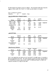 Table VI shows the ANOVA for the stepwise regression of the linear model.
Table VI: pH Response ANOVA
Response: pH
Stepwise Regression with Alpha to Enter = 0.100, Alpha to Exit = 0.100
Intercept
Forced
Terms:
Added
C-Surfactant
F Value
121.86
p-value
Prob > F
0.0001
R2
0.8266
MSE
0.081
ANOVA for Response Surface Reduced Linear Model
Analysis of Variance Table [Classical Sum-of-Squares - Type II]
Source
Model
C-Surfactant
Residual
Sum-of-
Squares
88.4
88.4
18.54
df
9
9
230
Mean
Square
9.82
9.82
0.081
F Value
121.86
121.86
p-value
Prob > F
< 0.0001
< 0.0001
significant
Lack-of-Fit
Pure
Experimental
Uncertainty
Cor Total
12
6.54
106.94
140
90
239
0.086
0.073
1.18
0.1986
not
significant
Std. Dev.
Mean
C.V. %
PRESS
0.28
5.95
4.77
20.19
R"
AdjR2
Pred R2
Adeq Precision
0.8266
0.8199
0.8112
37.625
Surfactant type is the only significant factor added to the linear model, which is also
significant at Prob>F of O.0001. There is only a 0.01% chance that a model F-value this
large could occur due to residual variance. The lack of fit F-value of 1.18 implies that the
lack-of-fit is not significant relative to the purely experimental uncertainty. There is a
19.86% chance that a significant lack-of-fit could occur due to purely experimental
uncertainty. The Pred-R2 of 0.8112 is in reasonable agreement with the Adj-R2 of 0.8199.
The signal-to-noise ratio, as is measured by Adeq. Precision, is greater than four and is
desirable. The ANOVA shows a ratio of 37.625, which indicates an adequate signal.
22
image:
Table VI shows the ANOVA for the stepwise regression of the linear model.
Table VI: pH Response ANOVA
Response: pH
Stepwise Regression with Alpha to Enter = 0.100, Alpha to Exit = 0.100
Intercept
Forced
Terms:
Added
C-Surfactant
F Value
121.86
p-value
Prob > F
0.0001
R2
0.8266
MSE
0.081
ANOVA for Response Surface Reduced Linear Model
Analysis of Variance Table [Classical Sum-of-Squares - Type II]
Source
Model
C-Surfactant
Residual
Sum-of-
Squares
88.4
88.4
18.54
df
9
9
230
Mean
Square
9.82
9.82
0.081
F Value
121.86
121.86
p-value
Prob > F
< 0.0001
< 0.0001
significant
Lack-of-Fit
Pure
Experimental
Uncertainty
Cor Total
12
6.54
106.94
140
90
239
0.086
0.073
1.18
0.1986
not
significant
Std. Dev.
Mean
C.V. %
PRESS
0.28
5.95
4.77
20.19
R"
AdjR2
Pred R2
Adeq Precision
0.8266
0.8199
0.8112
37.625
Surfactant type is the only significant factor added to the linear model, which is also
significant at Prob>F of O.0001. There is only a 0.01% chance that a model F-value this
large could occur due to residual variance. The lack of fit F-value of 1.18 implies that the
lack-of-fit is not significant relative to the purely experimental uncertainty. There is a
19.86% chance that a significant lack-of-fit could occur due to purely experimental
uncertainty. The Pred-R2 of 0.8112 is in reasonable agreement with the Adj-R2 of 0.8199.
The signal-to-noise ratio, as is measured by Adeq. Precision, is greater than four and is
desirable. The ANOVA shows a ratio of 37.625, which indicates an adequate signal.
22
image:
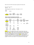 The ANOVA assumptions were now examined by inspecting the Residual Analysis
and Diagnostic plots. First, the check for normality was investigated in the normal
probability plot of the residuals for the pH response shown in Figure 7, pH Response
Diagnostics. The Normal Plot of the Residuals (Fig. 7A) should display a straight or near
straight line. Instead, the pH normal plot of the residuals shows an 'S' shape, which is not
linear and does not support the ANOVA assumption of normality. Furthermore, inspection
of the Residual vs. Predicted plot (Fig. 7B) does not reveal a random scatter, but rather a
horizontal hour-glass shape, which represents bias in the response and does not support the
ANOVA assumptions. Finally, the Predicted vs. Actual plot (Fig. 7C) does not support
A)
80-
70-
30-
20-
10-
5 -
B)
1
i
1 '
-1S7
MonaiyS
C)
I
523
I
7.05
Figure 7. pH Response Diagnostics A) Normal Plot of Internally Studentized Residuals, B) Internally
Studentized Residuals vs. Predicted, C) Predicted vs. Actual
random points scattered along the 45° line. The Predicted vs. Actual plot reveals poor
prediction as the points are clustered in groups above and below the line indicating areas of
23
image:
The ANOVA assumptions were now examined by inspecting the Residual Analysis
and Diagnostic plots. First, the check for normality was investigated in the normal
probability plot of the residuals for the pH response shown in Figure 7, pH Response
Diagnostics. The Normal Plot of the Residuals (Fig. 7A) should display a straight or near
straight line. Instead, the pH normal plot of the residuals shows an 'S' shape, which is not
linear and does not support the ANOVA assumption of normality. Furthermore, inspection
of the Residual vs. Predicted plot (Fig. 7B) does not reveal a random scatter, but rather a
horizontal hour-glass shape, which represents bias in the response and does not support the
ANOVA assumptions. Finally, the Predicted vs. Actual plot (Fig. 7C) does not support
A)
80-
70-
30-
20-
10-
5 -
B)
1
i
1 '
-1S7
MonaiyS
C)
I
523
I
7.05
Figure 7. pH Response Diagnostics A) Normal Plot of Internally Studentized Residuals, B) Internally
Studentized Residuals vs. Predicted, C) Predicted vs. Actual
random points scattered along the 45° line. The Predicted vs. Actual plot reveals poor
prediction as the points are clustered in groups above and below the line indicating areas of
23
image:
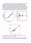 over or under prediction. Because these diagnostic plots reveal the linear model
assumptions are invalid and fail to support the ANOVA assumptions, the pH response is
not used as a predictable response in this investigation.
3.4 Conductivity Response
The conductivity response was first investigated for the need of a transform. The
response ranges from 0.968 to 7610 with a maximum-to-minimum ratio of 7861.57. A
ratio of 10 usually indicates that a transformation is required, so the Box-Cox plot was next
inspected. Figure 8 shows the Box-Cox plot for the Conductivity Response.
(Cond)"0.5
Lambda
Current = 0.5
Best =0.5
Low C.I. = 0.44
Hgh C.I. = 0.56
Recommend transform:
Square Root
{Lambda = 0.5)
Figure 8. Conductivity Box-Cox Plot
Laroooa
From inspection of the Box-Cox plot, it is recommended that a power transform with
0.5 (i.e., square root) is used to transform the response data. Therefore, the following
analysis is completed on the square root transformed conductivity response.
24
image:
over or under prediction. Because these diagnostic plots reveal the linear model
assumptions are invalid and fail to support the ANOVA assumptions, the pH response is
not used as a predictable response in this investigation.
3.4 Conductivity Response
The conductivity response was first investigated for the need of a transform. The
response ranges from 0.968 to 7610 with a maximum-to-minimum ratio of 7861.57. A
ratio of 10 usually indicates that a transformation is required, so the Box-Cox plot was next
inspected. Figure 8 shows the Box-Cox plot for the Conductivity Response.
(Cond)"0.5
Lambda
Current = 0.5
Best =0.5
Low C.I. = 0.44
Hgh C.I. = 0.56
Recommend transform:
Square Root
{Lambda = 0.5)
Figure 8. Conductivity Box-Cox Plot
Laroooa
From inspection of the Box-Cox plot, it is recommended that a power transform with
0.5 (i.e., square root) is used to transform the response data. Therefore, the following
analysis is completed on the square root transformed conductivity response.
24
image:
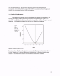 Using this transform, based on the Conductivity Response Fit Summary (Table VII), no
models are aliased and the linear or cubic model is suggested.
Table VII: Conductivity Response Fit Summary
Response: Conductivity
Transform:
Power
Lambda:
0.5 Constant:
Sequential Model Sum-of-Squares [Type I]
Source
Sum-of-
Squares
df
Mean
Square
F
Value
p-value
Prob > F
Mean vs. Total
Linear vs. Mean
2FI vs. Linear
Quadratic vs. 2FI
Cubic vs.
Quadratic
Residual
Total
1.20E+05
1.53E+05
86.14
1.48
101.82
315.7
2.73E+05
1
12
29
1
30
167
240
1.20E+05
12772
2.97
1.48
3.39
1.89
1138.94
5739.53
1.4
0.7
1.8
< 0.0001
0.0929
0.4043
Suggested
0.0111 Suggested
Lack-of-Fit Tests
Source
Linear
2FI
Quadratic
Cubic
Pure
Experimental
Uncertainty
Sum of
Squares
272.02
185.88
184.4
82.59
233.12
df
137
108
107
77
90
Mean
Square
1.99
1.72
1.72
1.07
2.59
F
Value
0.77
0.66
0.67
0.41
p-value
Prob > F
0.9202
0.9789
0.9783
1
Suggested
Suggested
Model Summary Statistics
Source
Linear
2FI
Quadratic
Cubic
Std. Dev.
1.49
1.45
1.46
1.37
R2
0.9967
0.9973
0.9973
0.9979
Adjusted
R2
0.9965
0.9967
0.9967
0.9971
Predicted
R2
0.9963
0.9958
0.9957
0.995
PRESS
566.87
651
655.64
776.03
Suggested
Suggested
Both models have acceptable Prob>F values and their respective lack-of-fit tests are
insignificant. The linear model Adj-R2 and Pred-R2 are 0.9965 and 0.9963, and the cubic
models are 0.9971 and 0.995, respectively. Both are very high and within ±0.2 of each
other. The normal plots of the internally studentized residuals for both models were
compared to evaluate which model to choose.
25
image:
Using this transform, based on the Conductivity Response Fit Summary (Table VII), no
models are aliased and the linear or cubic model is suggested.
Table VII: Conductivity Response Fit Summary
Response: Conductivity
Transform:
Power
Lambda:
0.5 Constant:
Sequential Model Sum-of-Squares [Type I]
Source
Sum-of-
Squares
df
Mean
Square
F
Value
p-value
Prob > F
Mean vs. Total
Linear vs. Mean
2FI vs. Linear
Quadratic vs. 2FI
Cubic vs.
Quadratic
Residual
Total
1.20E+05
1.53E+05
86.14
1.48
101.82
315.7
2.73E+05
1
12
29
1
30
167
240
1.20E+05
12772
2.97
1.48
3.39
1.89
1138.94
5739.53
1.4
0.7
1.8
< 0.0001
0.0929
0.4043
Suggested
0.0111 Suggested
Lack-of-Fit Tests
Source
Linear
2FI
Quadratic
Cubic
Pure
Experimental
Uncertainty
Sum of
Squares
272.02
185.88
184.4
82.59
233.12
df
137
108
107
77
90
Mean
Square
1.99
1.72
1.72
1.07
2.59
F
Value
0.77
0.66
0.67
0.41
p-value
Prob > F
0.9202
0.9789
0.9783
1
Suggested
Suggested
Model Summary Statistics
Source
Linear
2FI
Quadratic
Cubic
Std. Dev.
1.49
1.45
1.46
1.37
R2
0.9967
0.9973
0.9973
0.9979
Adjusted
R2
0.9965
0.9967
0.9967
0.9971
Predicted
R2
0.9963
0.9958
0.9957
0.995
PRESS
566.87
651
655.64
776.03
Suggested
Suggested
Both models have acceptable Prob>F values and their respective lack-of-fit tests are
insignificant. The linear model Adj-R2 and Pred-R2 are 0.9965 and 0.9963, and the cubic
models are 0.9971 and 0.995, respectively. Both are very high and within ±0.2 of each
other. The normal plots of the internally studentized residuals for both models were
compared to evaluate which model to choose.
25
image:
 A)
a.
*
• 672353
096387
B)
99-
95
90
80
70
-1223 -8.76 -5.26
internal Stuaenu zed net4fluan
I
1.80
1£7
95
90
80
70
50 -i
30
20
10
5
-10.71
I
•224
200
624
intern ary SUOMUM NcdduM
Figure 9. Conductivity Normal Plot of Internally Studentized Residuals A) Linear Model, B) Cubic Model
These plots are included in Figure 9, Conductivity Normal Plot of Internally Studentized
Residuals: Linear and Cubic Model. The linear model normal plot of the residuals (Fig.
9A) displays a straighter line than the cubic model (Fig. 9B) and, therefore, supports the
normality assumption for the ANOVA. Thus, the linear model was chosen to model the
transformed conductivity data. Again, the stepwise regression algorithm is used for the
power transformed lambda = 0.5, linear model, conductivity response ANOVA. The
results from this analysis are shown in Table VIII.
26
image:
A)
a.
*
• 672353
096387
B)
99-
95
90
80
70
-1223 -8.76 -5.26
internal Stuaenu zed net4fluan
I
1.80
1£7
95
90
80
70
50 -i
30
20
10
5
-10.71
I
•224
200
624
intern ary SUOMUM NcdduM
Figure 9. Conductivity Normal Plot of Internally Studentized Residuals A) Linear Model, B) Cubic Model
These plots are included in Figure 9, Conductivity Normal Plot of Internally Studentized
Residuals: Linear and Cubic Model. The linear model normal plot of the residuals (Fig.
9A) displays a straighter line than the cubic model (Fig. 9B) and, therefore, supports the
normality assumption for the ANOVA. Thus, the linear model was chosen to model the
transformed conductivity data. Again, the stepwise regression algorithm is used for the
power transformed lambda = 0.5, linear model, conductivity response ANOVA. The
results from this analysis are shown in Table VIII.
26
image:
 Table VIII: Conductivity Response ANOVA
Response: Conductivity
Transform: Power Lambda: 0.5 Constant: 0
Stepwise Regression with Alpha to Enter = 0.100, Alpha to Exit = 0.100
Forced
Terms:
Intercept
Added
C-Surfactant
B-Dye
F
Value
6793.8
15.42
p-value
Prob > F
0.0001
0.0001
R-Squared
0.9963
0.9967
MSE
2.51
2.23
ANOVA for Response Surface Reduced Linear Model
Analysis of Variance Table [Classical Sum-of-Squares - Type II]
Source
Model
B-Dye
C-Surfactant
Residual
Lack of Fit
Pure
Experimental
Uncertainty
Cor Total
Std. Dev.
Mean
C.V. %
PRESS
Sum-of-
Squares
1.53E+05
68.66
1.53E+05
507.59
274.47
233.12
1.54E+05
1.49
22.32
6.68
562.42
df .
11
2
9-
228
138
90
239
R2
AdjR2
Pred R2
Adeq Precision
Mean
Square
13932.86
34.33
17021.43
2.23
1.99
2.59
0.9967
0.9965
0.9963
252.665
F
Value
6258.44
15.42
7645.78
0.77
p-value
Prob > F
< 0.0001
< 0.0001
< 0.0001
0.9192
significant
not significant
The model F-value of 6258.44 implies that the model is significant and there is only a
0.01% chance that a "model F-value" this large could occur due to residual variance.
Values of Prob>F less than 0.05 (set as an arbitrary level) are used to indicate that the
model terms are significant. Only factor terms which meet this criterion are added to the
model per the stepwise regression procedure. In this case, terms B-dye type and C-
surfactant type are significant model factor terms. The lack-of-fit F-value of 0.77 implies
that the lack-of-fit is not significant relative to the purely experimental uncertainty. That is,
there is a 91.92% chance that a lack of fit F-value this large could occur due to purely
experimental uncertainty. This implies that the model fits the data. The Pred-R2 value of
0.9963 is in good agreement with the Adj-R2 value of 0.9965. The signal strength
indicated by the signal-to-noise ratio given by the adequate precision calculation is
27
image:
Table VIII: Conductivity Response ANOVA
Response: Conductivity
Transform: Power Lambda: 0.5 Constant: 0
Stepwise Regression with Alpha to Enter = 0.100, Alpha to Exit = 0.100
Forced
Terms:
Intercept
Added
C-Surfactant
B-Dye
F
Value
6793.8
15.42
p-value
Prob > F
0.0001
0.0001
R-Squared
0.9963
0.9967
MSE
2.51
2.23
ANOVA for Response Surface Reduced Linear Model
Analysis of Variance Table [Classical Sum-of-Squares - Type II]
Source
Model
B-Dye
C-Surfactant
Residual
Lack of Fit
Pure
Experimental
Uncertainty
Cor Total
Std. Dev.
Mean
C.V. %
PRESS
Sum-of-
Squares
1.53E+05
68.66
1.53E+05
507.59
274.47
233.12
1.54E+05
1.49
22.32
6.68
562.42
df .
11
2
9-
228
138
90
239
R2
AdjR2
Pred R2
Adeq Precision
Mean
Square
13932.86
34.33
17021.43
2.23
1.99
2.59
0.9967
0.9965
0.9963
252.665
F
Value
6258.44
15.42
7645.78
0.77
p-value
Prob > F
< 0.0001
< 0.0001
< 0.0001
0.9192
significant
not significant
The model F-value of 6258.44 implies that the model is significant and there is only a
0.01% chance that a "model F-value" this large could occur due to residual variance.
Values of Prob>F less than 0.05 (set as an arbitrary level) are used to indicate that the
model terms are significant. Only factor terms which meet this criterion are added to the
model per the stepwise regression procedure. In this case, terms B-dye type and C-
surfactant type are significant model factor terms. The lack-of-fit F-value of 0.77 implies
that the lack-of-fit is not significant relative to the purely experimental uncertainty. That is,
there is a 91.92% chance that a lack of fit F-value this large could occur due to purely
experimental uncertainty. This implies that the model fits the data. The Pred-R2 value of
0.9963 is in good agreement with the Adj-R2 value of 0.9965. The signal strength
indicated by the signal-to-noise ratio given by the adequate precision calculation is
27
image:
 252.665, which is an adequate signal represented by this model, because values greater
than four are used to indicate adequate model discrimination.
The normal plot of the internally studentized residuals for the linear model is shown
in Figure 9A. This plot shows the favorable straight line and support of normality. The
observation of the one data point at approximately -12.23 will be investigated further as a
possible outlier. The Conductivity Response Diagnostics Plots (Fig. 10) were investigated
to verify the ANOVA model assumptions.
A)
a 96387
(Cond)*0 5
B)
I
64S7
35 69 103 137 171 205 239
C)
I
4,11
Figure 10. Conductivity Response Diagnostic Plots A) Internally Studentized Residuals vs. Predicted, B)
Internally Studentized Residuals vs. Run, C) Predicted vs. Actual
28
image:
252.665, which is an adequate signal represented by this model, because values greater
than four are used to indicate adequate model discrimination.
The normal plot of the internally studentized residuals for the linear model is shown
in Figure 9A. This plot shows the favorable straight line and support of normality. The
observation of the one data point at approximately -12.23 will be investigated further as a
possible outlier. The Conductivity Response Diagnostics Plots (Fig. 10) were investigated
to verify the ANOVA model assumptions.
A)
a 96387
(Cond)*0 5
B)
I
64S7
35 69 103 137 171 205 239
C)
I
4,11
Figure 10. Conductivity Response Diagnostic Plots A) Internally Studentized Residuals vs. Predicted, B)
Internally Studentized Residuals vs. Run, C) Predicted vs. Actual
28
image:
 A)
3.00
-OB1 -
-462-
-842 -
(Cond)"OS -1223-
I I ! I I
i i i i i i
33 67 100 133 167 200
-031-
-462-
I
!
-8.42-
|«7236S
•!«»
(CmdpOS -1223-
J
J
•
1
I
J
\
•
-OB1-
-4*2-
-8.42 -
•08B38T
comi-os -1223-
11!! 111' i i
Figure 10 contains the rest of the
Conductivity Response Diagnostic
Plots. The Internally Studentized
Residual vs. Predicted plot (Fig.
1OA) should appear as a random
scatter, which it does. Again, the
presence a possible outlier is
observed. The Internally
Studentized Residual vs. Run Plot
(Fig. 1 OB) does not reveal a trend,
but rather shows a random scatter
(again, note the same possible
outlier). The model points are
scattered along the 45° line in the
Predicted vs. Actual plot (Fig. IOC)
with no groupings above or below
the line (again, note the same
possible outlier). These plots
support the ANOVA assumptions
and do not present any bias in the
model predictions. Next to be
inspected were the Internally
Studentized Residual vs. Factor Plots
in Figure 11. All three Residual vs.
Factor Plots (i.e., PCE cone.-Fig.
11 A, Dye-Fig. 1 IB, and Surfactant-
Fig. 11C) show an even distribution
of model points about the zero-line.
Upon inspection of the plots, there
are no obvious excessive points of
influence, which is good for the
ANOVA results.
1234587
10
Figure 11. Conductivity Response: Internally Studentized
Residuals vs. Factors A) Internally Studentized Residuals
vs. PCE concentration, B) Internally Studentized Residuals
vs. Dye, C) Residuals vs. Surfactant
29
image:
A)
3.00
-OB1 -
-462-
-842 -
(Cond)"OS -1223-
I I ! I I
i i i i i i
33 67 100 133 167 200
-031-
-462-
I
!
-8.42-
|«7236S
•!«»
(CmdpOS -1223-
J
J
•
1
I
J
\
•
-OB1-
-4*2-
-8.42 -
•08B38T
comi-os -1223-
11!! 111' i i
Figure 10 contains the rest of the
Conductivity Response Diagnostic
Plots. The Internally Studentized
Residual vs. Predicted plot (Fig.
1OA) should appear as a random
scatter, which it does. Again, the
presence a possible outlier is
observed. The Internally
Studentized Residual vs. Run Plot
(Fig. 1 OB) does not reveal a trend,
but rather shows a random scatter
(again, note the same possible
outlier). The model points are
scattered along the 45° line in the
Predicted vs. Actual plot (Fig. IOC)
with no groupings above or below
the line (again, note the same
possible outlier). These plots
support the ANOVA assumptions
and do not present any bias in the
model predictions. Next to be
inspected were the Internally
Studentized Residual vs. Factor Plots
in Figure 11. All three Residual vs.
Factor Plots (i.e., PCE cone.-Fig.
11 A, Dye-Fig. 1 IB, and Surfactant-
Fig. 11C) show an even distribution
of model points about the zero-line.
Upon inspection of the plots, there
are no obvious excessive points of
influence, which is good for the
ANOVA results.
1234587
10
Figure 11. Conductivity Response: Internally Studentized
Residuals vs. Factors A) Internally Studentized Residuals
vs. PCE concentration, B) Internally Studentized Residuals
vs. Dye, C) Residuals vs. Surfactant
29
image:
 Next, the presence of any outliers was examined with Influence plots (Fig. 12). The
Externally Studentized Residuals (or outlier-t values - Fig. 12A) reveal any points outside
the 95% confidence limits.
A)
•-14
.87.2353
•0.98387
(Cond}A0.5
B)
• 87.2J53
1096387
(Cond)A0.5:
1 35 69 103 137 171 205 239
RwMHMr
103 137 171 205 239
•MI
0.98387
(Cond)*0.5:
D)
0.98387
{Condro.5:
35 69 103 137 171 205 239
35 69 103 137 171 205 239
Figure 12. Conductivity Response Influence Plots A) Externally Studentized Residuals, B) DFFITS vs. Run,
C) Cook's Distance, D) Leverage vs. Run
This plot reveals that run #14 is located well beyond the lower 95% confidence limit and
requires that run #14 be investigated for possible error and as an outlier (this is the same
outlier identified in the earlier plots above). The DFFITS vs. Run (Fig. 12B) also exposes
run #14 from the other 240 experimental runs. Based on these two plots, run #14 may be
an influential run. The Cook's Distance plot (Fig. 12C) also shows this run as separate
from the other group of runs; however, this point does not exceed the approximate
threshold of one. This threshold is used as a flag for an outlier per the Cook's Distance plot
(see Appendix G for definition). Finally, the Leverage vs. Run plot (Fig. 12D) does not
show this point, or any model point, as yielding excessive leverage on the results. Run #14
30
image:
Next, the presence of any outliers was examined with Influence plots (Fig. 12). The
Externally Studentized Residuals (or outlier-t values - Fig. 12A) reveal any points outside
the 95% confidence limits.
A)
•-14
.87.2353
•0.98387
(Cond}A0.5
B)
• 87.2J53
1096387
(Cond)A0.5:
1 35 69 103 137 171 205 239
RwMHMr
103 137 171 205 239
•MI
0.98387
(Cond)*0.5:
D)
0.98387
{Condro.5:
35 69 103 137 171 205 239
35 69 103 137 171 205 239
Figure 12. Conductivity Response Influence Plots A) Externally Studentized Residuals, B) DFFITS vs. Run,
C) Cook's Distance, D) Leverage vs. Run
This plot reveals that run #14 is located well beyond the lower 95% confidence limit and
requires that run #14 be investigated for possible error and as an outlier (this is the same
outlier identified in the earlier plots above). The DFFITS vs. Run (Fig. 12B) also exposes
run #14 from the other 240 experimental runs. Based on these two plots, run #14 may be
an influential run. The Cook's Distance plot (Fig. 12C) also shows this run as separate
from the other group of runs; however, this point does not exceed the approximate
threshold of one. This threshold is used as a flag for an outlier per the Cook's Distance plot
(see Appendix G for definition). Finally, the Leverage vs. Run plot (Fig. 12D) does not
show this point, or any model point, as yielding excessive leverage on the results. Run #14
30
image:
 A)
No Surfactant -
5%Dow*xB390 -
0.5*. Dow** 8390-
0.1%SbolCS-330 -
S 0-025SS»olCS-330_
A 8% AMA-80-I —
05K.AMA-80-I -
50mMTween60 -
4%Tween80-MO%ECH-
4%T»een80 -
I
none
I
BB.
B)
Interaction
PCE conc= 10000
•C 4% -««r, 80
AC24% Twwi 90 + 10% ElCM
*C350mM T*«r60
•C-t n M- AMA 6T-i
Mcs e% AMA-arvi
MC6 f- 02S% Stetf CS-330
»c-
•
AC9 5% Cwfa« 8390
*ClO No Sur'aclart
66DOO-
22.000-
oooo-
t
C)
Interaction
PCC cone = 100.00 68.000 ~~
i i r
^ /y „*> ^ rfrxy ^ x
/7///////S
& o- a"
Figure 13. Conductivity Model Response Plots at 100 ppm PCE A)
Surfactant vs. Dye Matrix, B) Conductivity vs. Dye per Surfactant
Interaction Plot C) Conductivity vs. Surfactant per Dye Interaction
Plot
is, therefore, further investigated
through the inspection of the raw
data. This particular run was part
of a large group of points run on a
single day, and nothing in the
experimental procedure or daily
laboratory log notes anything
abnormal or odd about this data
point. Since no experimental
reason can be determined to flag
this data point and the Cook's
Distance and Leverage vs. Run
plots do not support this data
point as an outlier, run #14 is not
considered to be an outlier and
remains in the model and in the
analysis of the data.
Figure 13, Conductivity
Model Response Plots, shows the
three conductivity response
(transformed) plots. The
midrange concentration of 100
ppm PCE was chosen for the
evaluation because PCE was not
found to be a significant factor in
the stepwise regression ANOVA
for the conductivity response.
First is the matrix display of the
Conductivity of Surfactant type
vs. dye type (Fig., 13A). This
matrix can be navigated to inspect
the model response per each
surfactant and dye type tested.
The interaction plot of
(Conductivity)0 vs. Dye per
Surfactant at 100 ppm PCE (Fig.
13B) shows that the effect of dye
on the (conductivity)0 5 is very
small. Lastly, from Figure 13C
the magnitude of the conductivity
per surfactant can easily be
determined at 100 ppm PCE. The
order of surfactant type from most
electrically conductive to least
conductive is: 8% AMA-80-I, 5%
Dowfax 8390, 0.5% AMA-80-I,
31
image:
A)
No Surfactant -
5%Dow*xB390 -
0.5*. Dow** 8390-
0.1%SbolCS-330 -
S 0-025SS»olCS-330_
A 8% AMA-80-I —
05K.AMA-80-I -
50mMTween60 -
4%Tween80-MO%ECH-
4%T»een80 -
I
none
I
BB.
B)
Interaction
PCE conc= 10000
•C 4% -««r, 80
AC24% Twwi 90 + 10% ElCM
*C350mM T*«r60
•C-t n M- AMA 6T-i
Mcs e% AMA-arvi
MC6 f- 02S% Stetf CS-330
»c-
•
AC9 5% Cwfa« 8390
*ClO No Sur'aclart
66DOO-
22.000-
oooo-
t
C)
Interaction
PCC cone = 100.00 68.000 ~~
i i r
^ /y „*> ^ rfrxy ^ x
/7///////S
& o- a"
Figure 13. Conductivity Model Response Plots at 100 ppm PCE A)
Surfactant vs. Dye Matrix, B) Conductivity vs. Dye per Surfactant
Interaction Plot C) Conductivity vs. Surfactant per Dye Interaction
Plot
is, therefore, further investigated
through the inspection of the raw
data. This particular run was part
of a large group of points run on a
single day, and nothing in the
experimental procedure or daily
laboratory log notes anything
abnormal or odd about this data
point. Since no experimental
reason can be determined to flag
this data point and the Cook's
Distance and Leverage vs. Run
plots do not support this data
point as an outlier, run #14 is not
considered to be an outlier and
remains in the model and in the
analysis of the data.
Figure 13, Conductivity
Model Response Plots, shows the
three conductivity response
(transformed) plots. The
midrange concentration of 100
ppm PCE was chosen for the
evaluation because PCE was not
found to be a significant factor in
the stepwise regression ANOVA
for the conductivity response.
First is the matrix display of the
Conductivity of Surfactant type
vs. dye type (Fig., 13A). This
matrix can be navigated to inspect
the model response per each
surfactant and dye type tested.
The interaction plot of
(Conductivity)0 vs. Dye per
Surfactant at 100 ppm PCE (Fig.
13B) shows that the effect of dye
on the (conductivity)0 5 is very
small. Lastly, from Figure 13C
the magnitude of the conductivity
per surfactant can easily be
determined at 100 ppm PCE. The
order of surfactant type from most
electrically conductive to least
conductive is: 8% AMA-80-I, 5%
Dowfax 8390, 0.5% AMA-80-I,
31
image:
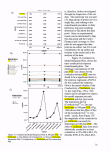 0.5% Dowfax 8390, 50 mM Tween 60,0.1% Steol CS-330, 4% Tween 80,4% Tween 80 +
10% EtOH, 0.025% Steol CS-330, and the No Surfactant. Additionally, these plots reveal
that, although dye type is statistically significant, inspection of the plots indicates that the
qualitative response to conductivity due to dye type is very minimal.
The final prediction model equation of the conductivity response determined by the
linear model in terms of the coded factors (B: dye type and C: surfactant type) is shown
below:
(Cond)05 =
+22.32
-0.25 * B[l]
+0.74 *B[2]
-15.35 *C[1]
-16.91 * C[2]
-12.05 * C[3]
+7.80 * C[4]
+62.98 * C[5]
-18.03 *C[6]
-14.01 * C[7]
-1.93 *C[8]
+27.59 * C[9]
With the following error analysis:
Term
Intercept
B[1]
B[2]
cm
C[2]
C[3]
C[4]
C[5]
C[6]
cm
C[8]
C[9]
Coefficient
Estimate
22.32
-0.25
0.74
-15.35
-16.91
-12.05
7.8
62.98
-18.03
-14.01
' -1.93
27.59
df
1
1
1
1
1
1
1
1
1
1
1
1
Standard
Error
0.096
0.14
0.14
0.29
0.29
0.29
0.29
0.29
0.29
0.29
0.29
0.29
95% Cl
Low
22.13
-0.52
0.48
-15.92
-17.48
-12.62
7.23
62.41
-18.59
-14.58
-2.5
27.02
95% Cl
High
22.51
0.016
1.01
-14.78
-16.34
-11.48
8.36
63.55
-17.46
-13.44
-1.36
28.16
This model can be used to predict the conductivity response due to the surfactant and dye
used.
32
image:
0.5% Dowfax 8390, 50 mM Tween 60,0.1% Steol CS-330, 4% Tween 80,4% Tween 80 +
10% EtOH, 0.025% Steol CS-330, and the No Surfactant. Additionally, these plots reveal
that, although dye type is statistically significant, inspection of the plots indicates that the
qualitative response to conductivity due to dye type is very minimal.
The final prediction model equation of the conductivity response determined by the
linear model in terms of the coded factors (B: dye type and C: surfactant type) is shown
below:
(Cond)05 =
+22.32
-0.25 * B[l]
+0.74 *B[2]
-15.35 *C[1]
-16.91 * C[2]
-12.05 * C[3]
+7.80 * C[4]
+62.98 * C[5]
-18.03 *C[6]
-14.01 * C[7]
-1.93 *C[8]
+27.59 * C[9]
With the following error analysis:
Term
Intercept
B[1]
B[2]
cm
C[2]
C[3]
C[4]
C[5]
C[6]
cm
C[8]
C[9]
Coefficient
Estimate
22.32
-0.25
0.74
-15.35
-16.91
-12.05
7.8
62.98
-18.03
-14.01
' -1.93
27.59
df
1
1
1
1
1
1
1
1
1
1
1
1
Standard
Error
0.096
0.14
0.14
0.29
0.29
0.29
0.29
0.29
0.29
0.29
0.29
0.29
95% Cl
Low
22.13
-0.52
0.48
-15.92
-17.48
-12.62
7.23
62.41
-18.59
-14.58
-2.5
27.02
95% Cl
High
22.51
0.016
1.01
-14.78
-16.34
-11.48
8.36
63.55
-17.46
-13.44
-1.36
28.16
This model can be used to predict the conductivity response due to the surfactant and dye
used.
32
image:
 3.5 Dissolved Oxygen Response
The necessity for a transform was first inspected. The range of DO response is
from a maximum of 10.48 to a minimum of 3.18 resulting in a ratio of 3.2956. Ratios less
than three result in power transforms having little effect. Because this ratio is slightly over
three, the Box-Cox analysis was investigated. Figure 14 shows the results of the Box-Cox
plot.
6.72 —
Lambda
Currert = 22
Best = 22 JJ
UwCI. = 1.77
HighCI. = 266
Reccmrrend transform:
Power S.
(Lanbda= 22) Y
Figure 14. Dissolved Oxygen Response Box-Cox Plot
This procedure recommends a power transform with lambda = 2.2. Therefore, the
dissolved oxygen data were analyzed with this power transform. Table IX: Dissolved
Oxygen Response Fit Summary shows the sequential model sum of squares, the lack-of-fit
tests, and the model summary statistics. These results suggest that the linear model is
significant with a Prob>F of 0.0001 and lack-of-fit as being insignificant at Prob>F of
0.9307. The Adj-R2 is within 0.2 of the Pred-R2 at 0.7801 and 0.7666, respectively.
33
image:
3.5 Dissolved Oxygen Response
The necessity for a transform was first inspected. The range of DO response is
from a maximum of 10.48 to a minimum of 3.18 resulting in a ratio of 3.2956. Ratios less
than three result in power transforms having little effect. Because this ratio is slightly over
three, the Box-Cox analysis was investigated. Figure 14 shows the results of the Box-Cox
plot.
6.72 —
Lambda
Currert = 22
Best = 22 JJ
UwCI. = 1.77
HighCI. = 266
Reccmrrend transform:
Power S.
(Lanbda= 22) Y
Figure 14. Dissolved Oxygen Response Box-Cox Plot
This procedure recommends a power transform with lambda = 2.2. Therefore, the
dissolved oxygen data were analyzed with this power transform. Table IX: Dissolved
Oxygen Response Fit Summary shows the sequential model sum of squares, the lack-of-fit
tests, and the model summary statistics. These results suggest that the linear model is
significant with a Prob>F of 0.0001 and lack-of-fit as being insignificant at Prob>F of
0.9307. The Adj-R2 is within 0.2 of the Pred-R2 at 0.7801 and 0.7666, respectively.
33
image:
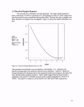 Table IX: Dissolved Oxygen Response Fit Summary
Response: DO Transform: Power Lambda:
Sequential Model Sum-of-Squares [Type I]
2.2
Constant: 0
Source
Mean vs. Total
Linear vs. Mean
2FI vs. Linear
Quadratic vs. 2FI
Cubic vs.
Quadratic
Residual
Total
Sum-of-
Squares
2.29E+06
2.40E+05
6379.08
52.63
7802.62
49208.4
2.60E+06
df
1
12
29
1
30
167
240
Mean
Square
2.29E+06
20030.54
219.97
52.63
260.09
294.66
10819.49
F
Value
71.67
0.76
0.18
0.88
p-value
Prob > F
< 0.0001
0.804
0.6702
0.645
Suggested
Lack-of-Fit Tests
Source
Linear
2FI
Quadratic
Cubic
Pure
Experimental
Uncertainty
Sum-of-
Squares
33941.48
27562.4
27509.77
19707.15
29501 .25
df
137
108
107
77
90
Mean
Square
247.75
. 255.21
257.1
255.94
327.79
F
Value
0.76
0.78
0.78
0.78
p-value
Prob > F
0.9307
0.8936
0.8862
0.8672
Suggested
Model Summary Statistics
Source
Linear
2FI
Quadratic
Cubic
Std. Dev.
16.72
16.98
17.01
17.17
R2
0.7912
0.8122
0.8123
0.838
Adjusted
R2
0.7801
0.7733
0.7723
0.7682
Predicted
R2
0.7666
0.7246
0.722
0.6618
PRESS
70910.26 Suggested
83670.52
84449.75
1 .03E+05
The linear model is chosen from these results to perform the stepwise ANOVA. These
results are shown in Table X: Dissolved Oxygen Response ANOVA. The stepwise
regression procedure added surfactant, dye, and PCE concentration to the linear model. All
of these factors are significant to the model response. Surfactant and Dye type resulted in a
Prob>F of 0.0001, and PCE concentration in a Prob>F of 0.0512. The ANOVA found the
model F-value of 71.67, which implies that the model is significant. There is a 0.01%
chance that a model F-value this large could occur due to residual variance. For the model
terms, values of Prob>F less than 0.0500 are used to indicate that the terms, B-dye and C-
surfactant, are significant. Terms which have Prob>F values greater than 0.1000 are used
to indicate that the model terms are insignificant.
34
image:
Table IX: Dissolved Oxygen Response Fit Summary
Response: DO Transform: Power Lambda:
Sequential Model Sum-of-Squares [Type I]
2.2
Constant: 0
Source
Mean vs. Total
Linear vs. Mean
2FI vs. Linear
Quadratic vs. 2FI
Cubic vs.
Quadratic
Residual
Total
Sum-of-
Squares
2.29E+06
2.40E+05
6379.08
52.63
7802.62
49208.4
2.60E+06
df
1
12
29
1
30
167
240
Mean
Square
2.29E+06
20030.54
219.97
52.63
260.09
294.66
10819.49
F
Value
71.67
0.76
0.18
0.88
p-value
Prob > F
< 0.0001
0.804
0.6702
0.645
Suggested
Lack-of-Fit Tests
Source
Linear
2FI
Quadratic
Cubic
Pure
Experimental
Uncertainty
Sum-of-
Squares
33941.48
27562.4
27509.77
19707.15
29501 .25
df
137
108
107
77
90
Mean
Square
247.75
. 255.21
257.1
255.94
327.79
F
Value
0.76
0.78
0.78
0.78
p-value
Prob > F
0.9307
0.8936
0.8862
0.8672
Suggested
Model Summary Statistics
Source
Linear
2FI
Quadratic
Cubic
Std. Dev.
16.72
16.98
17.01
17.17
R2
0.7912
0.8122
0.8123
0.838
Adjusted
R2
0.7801
0.7733
0.7723
0.7682
Predicted
R2
0.7666
0.7246
0.722
0.6618
PRESS
70910.26 Suggested
83670.52
84449.75
1 .03E+05
The linear model is chosen from these results to perform the stepwise ANOVA. These
results are shown in Table X: Dissolved Oxygen Response ANOVA. The stepwise
regression procedure added surfactant, dye, and PCE concentration to the linear model. All
of these factors are significant to the model response. Surfactant and Dye type resulted in a
Prob>F of 0.0001, and PCE concentration in a Prob>F of 0.0512. The ANOVA found the
model F-value of 71.67, which implies that the model is significant. There is a 0.01%
chance that a model F-value this large could occur due to residual variance. For the model
terms, values of Prob>F less than 0.0500 are used to indicate that the terms, B-dye and C-
surfactant, are significant. Terms which have Prob>F values greater than 0.1000 are used
to indicate that the model terms are insignificant.
34
image:
 Table X: Dissolved Oxygen Response ANOVA
Response: DO
Transform:
Power
Lambda: 2.2
Constant:
Stepwise Regression with Alpha to Enter = 0.100, Alpha to Exit = 0.100
Forced Terms: Intercept
Added
C-Surfactant
B-Dye
A-PCE cone
F
Value
81.06
14.67
3.84
p-value
Prob > F
0.0001
0.0001
0.0512
R-Squared
0.7603
0.7876
0.7912
MSE
316.61
282.97
279.48
ANOVA for Response Surface Linear Model
Analysis of Variance Table [Classical Sum-of-Squares - Type II]
Source
Model
A-PCE cone
B-Dye
C-Surfactant
Residual
Lack of Fit
Pure
Experimental
Uncertainty
Cor Total
Std. Dev.
Mean
C.V. %
PRESS
Sum-of-
Squares
2.40E+05
1073.81
8303.49
2.31 E+05
63442.73
33941.48
29501 .25
3.04E+05
16.72
97.74
17.1
70910.26
df
12
1
2
9
227
137
90
239
R2
AdjR2
Pred R2
Adeq Precision
Mean
Square
20030.54
1073.81
4151.75
25665.47
279.48
247.75
327.79
0.7912
0.7801
0.7666
28.035
F
Value
71.67
3.84
14.86
91.83
0.76
p-value
Prob > F
< 0.0001
0.0512
< 0.0001
< 0.0001
0.9307
significant
not
significant
The model term, A-PCE concentration, shows a Prob>F value greater than 0.0500, but less
than 0.1000; therefore this term is included in the model and determined to be significant.
The lack-of-fit value of 0.76 implies that the lack-of-fit is not significant relative to the
purely experimental uncertainty. There is a 93.07% chance that a lack of fit value this
large could occur due to noise. This is good and indicates the model fits. The Pred-R2 of
0.7666 is in reasonable agreement with the adjusted R2 of 0.7801. Adequate precision
ratios of greater than four are desirable in the signal-to-noise ratio. This model shows an
adequate precision of 28.035, indicating an adequate signal.
As in the previous responses, the ANOVA assumptions are evaluated through the
residual analysis and diagnostic plots. Figure 15 shows the DO Response Diagnostic Plots.
35
image:
Table X: Dissolved Oxygen Response ANOVA
Response: DO
Transform:
Power
Lambda: 2.2
Constant:
Stepwise Regression with Alpha to Enter = 0.100, Alpha to Exit = 0.100
Forced Terms: Intercept
Added
C-Surfactant
B-Dye
A-PCE cone
F
Value
81.06
14.67
3.84
p-value
Prob > F
0.0001
0.0001
0.0512
R-Squared
0.7603
0.7876
0.7912
MSE
316.61
282.97
279.48
ANOVA for Response Surface Linear Model
Analysis of Variance Table [Classical Sum-of-Squares - Type II]
Source
Model
A-PCE cone
B-Dye
C-Surfactant
Residual
Lack of Fit
Pure
Experimental
Uncertainty
Cor Total
Std. Dev.
Mean
C.V. %
PRESS
Sum-of-
Squares
2.40E+05
1073.81
8303.49
2.31 E+05
63442.73
33941.48
29501 .25
3.04E+05
16.72
97.74
17.1
70910.26
df
12
1
2
9
227
137
90
239
R2
AdjR2
Pred R2
Adeq Precision
Mean
Square
20030.54
1073.81
4151.75
25665.47
279.48
247.75
327.79
0.7912
0.7801
0.7666
28.035
F
Value
71.67
3.84
14.86
91.83
0.76
p-value
Prob > F
< 0.0001
0.0512
< 0.0001
< 0.0001
0.9307
significant
not
significant
The model term, A-PCE concentration, shows a Prob>F value greater than 0.0500, but less
than 0.1000; therefore this term is included in the model and determined to be significant.
The lack-of-fit value of 0.76 implies that the lack-of-fit is not significant relative to the
purely experimental uncertainty. There is a 93.07% chance that a lack of fit value this
large could occur due to noise. This is good and indicates the model fits. The Pred-R2 of
0.7666 is in reasonable agreement with the adjusted R2 of 0.7801. Adequate precision
ratios of greater than four are desirable in the signal-to-noise ratio. This model shows an
adequate precision of 28.035, indicating an adequate signal.
As in the previous responses, the ANOVA assumptions are evaluated through the
residual analysis and diagnostic plots. Figure 15 shows the DO Response Diagnostic Plots.
35
image:
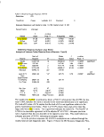 A)
12 74S
(OOr2.2
-2S2
-1.12
line
I
0.28
B)
2736 55.23 82.60
D)
1175 7M
12.745
(DO)A2.2
Run
Figure 15. Dissolved Oxygen Response Diagnostic Plots A) Normal Plot of Internally Studentized
Residuals, B) Internally Studentized Residuals vs. Predicted, C) Internally Studentized Residuals vs. Run, D)
Predicted vs. Actual
The Normal Plot of the Residuals (Fig. ISA) tests the normality assumption of the ANOVA
and should display the points on a straight line. The results show the majority of the
transformed DO response model points fit a straight line and therefore support the
normality assumption. The Residuals vs. Predicted plot (Fig. 15B) shows the random
scatter of points as does the Residuals vs. Run plot (Fig. 15C) implying that these plots
show no bias in the model prediction or in the run order used in the experiments. The
Predicted vs. Actual plot (Fig. 15D) shows a random scatter of points along the 45° line
with no bias or grouping of points above or below the line, thereby indicating that the
model shows good prediction. Next, the residuals vs. the individual model factors are
analyzed for random scatter split about the zero line.
36
image:
A)
12 74S
(OOr2.2
-2S2
-1.12
line
I
0.28
B)
2736 55.23 82.60
D)
1175 7M
12.745
(DO)A2.2
Run
Figure 15. Dissolved Oxygen Response Diagnostic Plots A) Normal Plot of Internally Studentized
Residuals, B) Internally Studentized Residuals vs. Predicted, C) Internally Studentized Residuals vs. Run, D)
Predicted vs. Actual
The Normal Plot of the Residuals (Fig. ISA) tests the normality assumption of the ANOVA
and should display the points on a straight line. The results show the majority of the
transformed DO response model points fit a straight line and therefore support the
normality assumption. The Residuals vs. Predicted plot (Fig. 15B) shows the random
scatter of points as does the Residuals vs. Run plot (Fig. 15C) implying that these plots
show no bias in the model prediction or in the run order used in the experiments. The
Predicted vs. Actual plot (Fig. 15D) shows a random scatter of points along the 45° line
with no bias or grouping of points above or below the line, thereby indicating that the
model shows good prediction. Next, the residuals vs. the individual model factors are
analyzed for random scatter split about the zero line.
36
image:
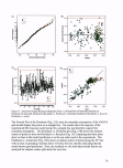 A)
» 175 709
12.745
(DOrZ2:
I
I
These data are shown in Figure 16,
Dissolved Oxygen Residuals vs.
Factors. Each of the three plots
show that the residuals are randomly
scattered about the zero line with no
bias or grouping of points above or
below the line per the responses
PCE concentration (Fig. 16A), Dye
(Fig. 16B), and Surfactant (Fig.
16C).
0 33 67 100 133 167 200
PCE cone
B)
.175.7
•12.74
C)
.175 709
•l2.745
(DOX-22
rnrf
•
. i., •
123456789 10
CMOMMt
Figure 16. Dissolved Oxygen Response Residuals vs. Factors.
A) Internally Studentized Residuals vs. PCE concentration, B)
Internally Studentized Residuals vs. Dye, C) Internally
Studentized Residuals vs. Surfactant
37
image:
A)
» 175 709
12.745
(DOrZ2:
I
I
These data are shown in Figure 16,
Dissolved Oxygen Residuals vs.
Factors. Each of the three plots
show that the residuals are randomly
scattered about the zero line with no
bias or grouping of points above or
below the line per the responses
PCE concentration (Fig. 16A), Dye
(Fig. 16B), and Surfactant (Fig.
16C).
0 33 67 100 133 167 200
PCE cone
B)
.175.7
•12.74
C)
.175 709
•l2.745
(DOX-22
rnrf
•
. i., •
123456789 10
CMOMMt
Figure 16. Dissolved Oxygen Response Residuals vs. Factors.
A) Internally Studentized Residuals vs. PCE concentration, B)
Internally Studentized Residuals vs. Dye, C) Internally
Studentized Residuals vs. Surfactant
37
image:
 t
103 137 171 205 239
nun Number
B)
|
1175.709
12745
(D0)*2.2
35 69 103 137 171 205 236
Run Number
-175.709
^ 12.745
(DO)* 2.2:
D)
103 137 171 205 239
103 137 171 205 23S
Figure 17. Dissolved Oxygen Response Influence Plots A) Externally Studentized Residuals, B) Leverage
vs. Run, C) DFFITS vs. Run, D) Cook's Distance
Next, the influence plots were analyzed to determine if outliers were present or if
circumstances allowed for the data points to have undue influence over the results. Figure
17 DO Response Influence Plots includes these analyses. The Externally Studentized
Residuals plot (Fig. 17A) shows the outlier t-values. The two red horizontal lines show the
95% confidence limits, in which all the points occur. This indicates that all of the data
points conform to the model and no points stand out. The Leverage vs. Run plot (Fig. 17B)
shows that no data points are beyond the average leverage. This is also good as it
demonstrates that there are no runs which unduly influence the model parameters. The
DFFITS vs. Run plot (Fig. 17C) shows that all of the points fall within the favorable +/-
2.00 difference in fits and, therefore, does not identify any influential runs. Finally, the
Cook's Distance plot (Fig. 17D) shows that all of the points conform and that no outliers
are present.
38
image:
t
103 137 171 205 239
nun Number
B)
|
1175.709
12745
(D0)*2.2
35 69 103 137 171 205 236
Run Number
-175.709
^ 12.745
(DO)* 2.2:
D)
103 137 171 205 239
103 137 171 205 23S
Figure 17. Dissolved Oxygen Response Influence Plots A) Externally Studentized Residuals, B) Leverage
vs. Run, C) DFFITS vs. Run, D) Cook's Distance
Next, the influence plots were analyzed to determine if outliers were present or if
circumstances allowed for the data points to have undue influence over the results. Figure
17 DO Response Influence Plots includes these analyses. The Externally Studentized
Residuals plot (Fig. 17A) shows the outlier t-values. The two red horizontal lines show the
95% confidence limits, in which all the points occur. This indicates that all of the data
points conform to the model and no points stand out. The Leverage vs. Run plot (Fig. 17B)
shows that no data points are beyond the average leverage. This is also good as it
demonstrates that there are no runs which unduly influence the model parameters. The
DFFITS vs. Run plot (Fig. 17C) shows that all of the points fall within the favorable +/-
2.00 difference in fits and, therefore, does not identify any influential runs. Finally, the
Cook's Distance plot (Fig. 17D) shows that all of the points conform and that no outliers
are present.
38
image:
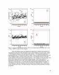 A)
XI = C: Surfactant
X2= 8: Dy«
Actual Factor
A PCE cone = 0.00
B)
Ongnal Scato
DO
• B2B B
B3 Ol-ftod-O
xi = C: Strfactat
X2 = B: Dy»
Actual Factor
A: PCE cone = 100.00
B DV*
C)
• B2B B
8301-Ftod-O
= C Si/factant
»B: Dya
Actual Factor
A: PCE cone a 200. 00
Sufactant
Figure 18. Dissolved Oxygen Model Response Interaction Plots.
A) DO vs. Surfactant per Dye type at 0 ppm PCE, B) DO vs.
Surfactant per Dye type at 100 ppm PCE, C) DO vs. Surfactant
per Dye type at 200 ppm PCE
The results of the dissolved oxygen
transformed response are shown in
the Dissolved Oxygen Response
Plots (Fig. 18). The response
figures are shown with the original
untransformed DO scale in order to
present the model response using
recognizable values of DO in mg/L.
The model response graphs show
the DO (mg/L) per surfactant for
each of the three dye treatments.
The three plots include the
interaction for 0 ppm PCE (Fig.
ISA), 100 ppm PCE (Fig. 18B),
and 200 ppm PCE (Fig. 18C).
Each plot shows lower DO
responses when using Oil-Red-O or
no dye vs. Brilliant Blue G-250. It
appears that the inclusion of
Brilliant Blue G-250 raises the DO
concentration slightly. Secondly,
in comparing the relative levels of
PCE concentration, the highest DO
values are seen with no PCE, while
the lowest are with the highest
concentration of PCE. This
apparent inverse relationship does
exist, but with a very small
magnitude. For example, the 4%
Tween 80 shows the lowest DO
response, while the 0.5% Dowfax
8390 shows the highest. The plots
reveal a group of surfactants which
form a plateau of the largest values
of DO (Fig. 18). These surfactants
include: 0.5% AMA-80-I, 8%
AMA-80-I, 0.025% Steol CS-330,
0.1% Steol CS-330, 0.5% Dowfax
8390, and 5% Dowfax 8390. Three
surfactants, 4% Tween 80, 4%
Tween 80 + 10% EtOH, and 50
mM Tween 60 were found to have
lower concentrations of DO than
the experiments with no surfactant
treatment.
39
image:
A)
XI = C: Surfactant
X2= 8: Dy«
Actual Factor
A PCE cone = 0.00
B)
Ongnal Scato
DO
• B2B B
B3 Ol-ftod-O
xi = C: Strfactat
X2 = B: Dy»
Actual Factor
A: PCE cone = 100.00
B DV*
C)
• B2B B
8301-Ftod-O
= C Si/factant
»B: Dya
Actual Factor
A: PCE cone a 200. 00
Sufactant
Figure 18. Dissolved Oxygen Model Response Interaction Plots.
A) DO vs. Surfactant per Dye type at 0 ppm PCE, B) DO vs.
Surfactant per Dye type at 100 ppm PCE, C) DO vs. Surfactant
per Dye type at 200 ppm PCE
The results of the dissolved oxygen
transformed response are shown in
the Dissolved Oxygen Response
Plots (Fig. 18). The response
figures are shown with the original
untransformed DO scale in order to
present the model response using
recognizable values of DO in mg/L.
The model response graphs show
the DO (mg/L) per surfactant for
each of the three dye treatments.
The three plots include the
interaction for 0 ppm PCE (Fig.
ISA), 100 ppm PCE (Fig. 18B),
and 200 ppm PCE (Fig. 18C).
Each plot shows lower DO
responses when using Oil-Red-O or
no dye vs. Brilliant Blue G-250. It
appears that the inclusion of
Brilliant Blue G-250 raises the DO
concentration slightly. Secondly,
in comparing the relative levels of
PCE concentration, the highest DO
values are seen with no PCE, while
the lowest are with the highest
concentration of PCE. This
apparent inverse relationship does
exist, but with a very small
magnitude. For example, the 4%
Tween 80 shows the lowest DO
response, while the 0.5% Dowfax
8390 shows the highest. The plots
reveal a group of surfactants which
form a plateau of the largest values
of DO (Fig. 18). These surfactants
include: 0.5% AMA-80-I, 8%
AMA-80-I, 0.025% Steol CS-330,
0.1% Steol CS-330, 0.5% Dowfax
8390, and 5% Dowfax 8390. Three
surfactants, 4% Tween 80, 4%
Tween 80 + 10% EtOH, and 50
mM Tween 60 were found to have
lower concentrations of DO than
the experiments with no surfactant
treatment.
39
image:
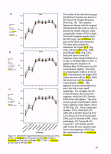 The final equation in terms of coded factors (A: PCE cone., B: dye type, C:
surfactant type) from the stepwise regression ANOVA for the linear model is:
(DO)2 2 =
+97.74
-2.82 * A
-5.07 *B[1]
+8.25 * B[2]
-61.89 *C[1]
-30.31 * C[2]
-39.13 * C[3]
+17.08 * C[4]
+25.32 * C[5]
+21.43*C[6]
+21.00*C[7]
+28.23 * C[8]
+25.67 * C[9]
With the following error, analysis:
Term
Intercept
A-PCE cone
B[1]
B[2]
C[1]
C[2]
C[3]
C[4]
C[5]
C[6]
C[7]
C[8]
C[9]
Coefficient
Estimate
97.74259
-2.82031
-5.06999
8.246234
-61.8936
-30.3078
-39.1298
17.08141
25.32061
21 .4343
21.00442
28.22826
25.66756
df
1
1
1
1
1
1
1
1
1
1
1
1
1
Standard
Error
1.079127
1.438835
1.526115
1.526115
3.23738
3.23738
3.23738
3.23738
3.23738
3.23738
3.23738
3.23738
3.23738
95% Cl
Low
95.61621
-5.65549
-8.07715
5.23907
-68.2728
-36.687
-45.509
10.70225
18.94145
15.05514
14.62526
21.8491
19.2884
95% Cl
High
99.86898
0.014875
-2.06282
1 1 .2534
-55.5145
-23.9287
-32.7507
23.46057
31.69977
27.81345
27.38358
34.60742
32.04672
VIF
1
40
image:
The final equation in terms of coded factors (A: PCE cone., B: dye type, C:
surfactant type) from the stepwise regression ANOVA for the linear model is:
(DO)2 2 =
+97.74
-2.82 * A
-5.07 *B[1]
+8.25 * B[2]
-61.89 *C[1]
-30.31 * C[2]
-39.13 * C[3]
+17.08 * C[4]
+25.32 * C[5]
+21.43*C[6]
+21.00*C[7]
+28.23 * C[8]
+25.67 * C[9]
With the following error, analysis:
Term
Intercept
A-PCE cone
B[1]
B[2]
C[1]
C[2]
C[3]
C[4]
C[5]
C[6]
C[7]
C[8]
C[9]
Coefficient
Estimate
97.74259
-2.82031
-5.06999
8.246234
-61.8936
-30.3078
-39.1298
17.08141
25.32061
21 .4343
21.00442
28.22826
25.66756
df
1
1
1
1
1
1
1
1
1
1
1
1
1
Standard
Error
1.079127
1.438835
1.526115
1.526115
3.23738
3.23738
3.23738
3.23738
3.23738
3.23738
3.23738
3.23738
3.23738
95% Cl
Low
95.61621
-5.65549
-8.07715
5.23907
-68.2728
-36.687
-45.509
10.70225
18.94145
15.05514
14.62526
21.8491
19.2884
95% Cl
High
99.86898
0.014875
-2.06282
1 1 .2534
-55.5145
-23.9287
-32.7507
23.46057
31.69977
27.81345
27.38358
34.60742
32.04672
VIF
1
40
image:
 3.6 Density Response
The density response was first inspected for the possibility of a transform. The
density response ranges from 0.982 to 1.02267, with a ratio of the maximum-to-minimum
of 1.04142. For ratios less than three, the power transforms have little effect and, for
thoroughness, the Box-Cox plot is shown in Figure 19, which confirms that no transform of
the data is suggested.
-4.589 -
Lambda
Current = 1
Best = 3
Low C.I. =
High C.I. =
Recommend
transform:
None
(Lambda = 1)
-4.593 -
-4.597-
I
-4.602 -
-4.606 -
Lambda
Figure 19. Density Response Box-Cox Plot
41
image:
3.6 Density Response
The density response was first inspected for the possibility of a transform. The
density response ranges from 0.982 to 1.02267, with a ratio of the maximum-to-minimum
of 1.04142. For ratios less than three, the power transforms have little effect and, for
thoroughness, the Box-Cox plot is shown in Figure 19, which confirms that no transform of
the data is suggested.
-4.589 -
Lambda
Current = 1
Best = 3
Low C.I. =
High C.I. =
Recommend
transform:
None
(Lambda = 1)
-4.593 -
-4.597-
I
-4.602 -
-4.606 -
Lambda
Figure 19. Density Response Box-Cox Plot
41
image:
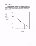 Table XI: Density Response Fit Summary
Response: density Transform:
Sequential Model Sum-of-Squares [Type I]
None
Source
Mean vs. Total
Linear vs. Mean
2FI vs. Linear
Quadratic vs. 2FI
Cubic vs. Quadratic
Residual
Total
Sum-of-
Squares
241.31
2.367E-03
1.845E-03
1.404E-05
1.114E-03
7.956E-03 .
241.32
df
1
12
29
1
30
167
240
Mean
Square
241.31
1 .973E-04
6.362E-05
1.404E-05
3.712E-05
4.764E-05
1.01
F
Value
4.10
1.39
0.30
0.78
p-value
Prob > F
< 0.0001
0.1009
0.5814
0.7870
Suggested
Suggested
Lack-of-Fit Tests
Source
Linear
2FI
Quadratic
Cubic
Pure Experimental
Uncertainty
Sum-of-
Squares
7.941 E-03
6.097E-03
6.083E-03
4.969E-03
2.987E-03
df
137
108
107
77
90
Mean
Square
5.797E-05
5.645E-05
5.685E-05
6.453E-05
3.319E-05
F
Value
1.75
1.70
1.71
1.94
p-value
Prob > F
0.0024
0.0049
0.0045
0.0012
Suggested
Suggested
Model Summary Statistics
Source
Linear
2FI
Quadratic
Cubic
Std. Dev.
6.983E-03
6.773E-03
6.785E-03
6.902E-03
R2
0.1781
0.3168
0.3179
0.4016
Adjusted
R2
0.1346
0.1754
0.1724
0.1437
Predicted
R2
0.0822
0.0144
0.0069
-0.1922
PRESS
0.012
0.013
0.013
0.016
Suggested
Suggested
Table XI includes the Density Response Fit Summary. The sequential model sum-of-
squares suggests both a linear and two factor interaction (2FI) model with a Prob>F of <
0.0001 and 0.1009, respectively. Additional results in the Fit Summary show a lack-of-fit
Prob > F of 0.0024 and 0.0049 for the linear and 2FI model, and the Adj-R2 is 0.1346 and
0.1754, respectively. Even though both models resulted in similar statistics; however, the
2FI model Adj-R2 is slightly higher, the 2FI model was chosen as this model is the highest
order polynomial where additional terms are shown to be significant and not aliased.
Therefore, the 2FI model was chosen and the ANOVA was performed using stepwise
regression.
42
image:
Table XI: Density Response Fit Summary
Response: density Transform:
Sequential Model Sum-of-Squares [Type I]
None
Source
Mean vs. Total
Linear vs. Mean
2FI vs. Linear
Quadratic vs. 2FI
Cubic vs. Quadratic
Residual
Total
Sum-of-
Squares
241.31
2.367E-03
1.845E-03
1.404E-05
1.114E-03
7.956E-03 .
241.32
df
1
12
29
1
30
167
240
Mean
Square
241.31
1 .973E-04
6.362E-05
1.404E-05
3.712E-05
4.764E-05
1.01
F
Value
4.10
1.39
0.30
0.78
p-value
Prob > F
< 0.0001
0.1009
0.5814
0.7870
Suggested
Suggested
Lack-of-Fit Tests
Source
Linear
2FI
Quadratic
Cubic
Pure Experimental
Uncertainty
Sum-of-
Squares
7.941 E-03
6.097E-03
6.083E-03
4.969E-03
2.987E-03
df
137
108
107
77
90
Mean
Square
5.797E-05
5.645E-05
5.685E-05
6.453E-05
3.319E-05
F
Value
1.75
1.70
1.71
1.94
p-value
Prob > F
0.0024
0.0049
0.0045
0.0012
Suggested
Suggested
Model Summary Statistics
Source
Linear
2FI
Quadratic
Cubic
Std. Dev.
6.983E-03
6.773E-03
6.785E-03
6.902E-03
R2
0.1781
0.3168
0.3179
0.4016
Adjusted
R2
0.1346
0.1754
0.1724
0.1437
Predicted
R2
0.0822
0.0144
0.0069
-0.1922
PRESS
0.012
0.013
0.013
0.016
Suggested
Suggested
Table XI includes the Density Response Fit Summary. The sequential model sum-of-
squares suggests both a linear and two factor interaction (2FI) model with a Prob>F of <
0.0001 and 0.1009, respectively. Additional results in the Fit Summary show a lack-of-fit
Prob > F of 0.0024 and 0.0049 for the linear and 2FI model, and the Adj-R2 is 0.1346 and
0.1754, respectively. Even though both models resulted in similar statistics; however, the
2FI model Adj-R2 is slightly higher, the 2FI model was chosen as this model is the highest
order polynomial where additional terms are shown to be significant and not aliased.
Therefore, the 2FI model was chosen and the ANOVA was performed using stepwise
regression.
42
image:
 Table XII: Density Response ANOVA
Response: density
Stepwise Regression with Alpha to Enter = 0.100, Alpha to Exit = 0.100
Forced Terms: Intercept
Added
C-Surfactant
AC
F
Value
5.416
2.309
p-value
Prob > F
0.0001
0.0168
R2
0.1749
0.2458
MSE
4.77E-05
4.54E-05
Hierarchical Terms Added after Stepwise Regression: A-PCE cone
ANOVA for Response Surface Reduced 2FI Model
Analysis of Variance Table [Classical Sum-of-Squares - Type II]
Source
Model
A-PCE cone
C-Surfactant
AC
Residual
Lack of Fit
Pure
Experimental
Uncertainty
Cor Total
Std. Dev.
Mean
C.V. %
PRESS
Sum-of-
Squares
3.27E-03
1.96E-07
2.33E-03 .
9.43E-04
0.01003
0.007
0.00299
0.01330
0.00675
1.00272
0.67329
0.01175
df
19
9
9
9
220
130
90
239
R2
AdjR2
Pred R2
Adeq Precision
Mean
Square
1.72E-04
1.96E-07
2.58E-04
0.00105
4.46E-05
5.42E-05
3.32E-05
0.2458
0.1807
0.1162
8.9601
F
Value
3.77
0.004
5.668
2.298
1.632
p-value
Prob > F
< 0.0001
0.9478
< 0.0001
0.0174
0.0069
significant
significant
These results are shown in Table XII: Density Response ANOVA. The Stepwise
regression procedure found that the surfactant (C) and the interaction between PCE
concentration and surfactant (AC) were statistically significant with the Prob>F being
O.0001 and 0.0174, respectively. Additionally, the model showed a significant Prob>F
value of O.0001. Thus, these two factors were included in the 2FI model. The lack-of-fit
test for this model found it significant with a F-value of 1.63 and a Prob>F of 0.0069
indicating that there is a 0.69% chance that a lack-of-fit F-value this large could be due to
purely experimental uncertainty. A higher lack-of-fit would be better as it is desirable that
the lack-of-fit is not significant. The Pred-R2 of 0.1162 is in reasonable agreement with the
Adj-R2 of 0.1807. The adequate precision ratio is 8.960, which indicates that the model
43
image:
Table XII: Density Response ANOVA
Response: density
Stepwise Regression with Alpha to Enter = 0.100, Alpha to Exit = 0.100
Forced Terms: Intercept
Added
C-Surfactant
AC
F
Value
5.416
2.309
p-value
Prob > F
0.0001
0.0168
R2
0.1749
0.2458
MSE
4.77E-05
4.54E-05
Hierarchical Terms Added after Stepwise Regression: A-PCE cone
ANOVA for Response Surface Reduced 2FI Model
Analysis of Variance Table [Classical Sum-of-Squares - Type II]
Source
Model
A-PCE cone
C-Surfactant
AC
Residual
Lack of Fit
Pure
Experimental
Uncertainty
Cor Total
Std. Dev.
Mean
C.V. %
PRESS
Sum-of-
Squares
3.27E-03
1.96E-07
2.33E-03 .
9.43E-04
0.01003
0.007
0.00299
0.01330
0.00675
1.00272
0.67329
0.01175
df
19
9
9
9
220
130
90
239
R2
AdjR2
Pred R2
Adeq Precision
Mean
Square
1.72E-04
1.96E-07
2.58E-04
0.00105
4.46E-05
5.42E-05
3.32E-05
0.2458
0.1807
0.1162
8.9601
F
Value
3.77
0.004
5.668
2.298
1.632
p-value
Prob > F
< 0.0001
0.9478
< 0.0001
0.0174
0.0069
significant
significant
These results are shown in Table XII: Density Response ANOVA. The Stepwise
regression procedure found that the surfactant (C) and the interaction between PCE
concentration and surfactant (AC) were statistically significant with the Prob>F being
O.0001 and 0.0174, respectively. Additionally, the model showed a significant Prob>F
value of O.0001. Thus, these two factors were included in the 2FI model. The lack-of-fit
test for this model found it significant with a F-value of 1.63 and a Prob>F of 0.0069
indicating that there is a 0.69% chance that a lack-of-fit F-value this large could be due to
purely experimental uncertainty. A higher lack-of-fit would be better as it is desirable that
the lack-of-fit is not significant. The Pred-R2 of 0.1162 is in reasonable agreement with the
Adj-R2 of 0.1807. The adequate precision ratio is 8.960, which indicates that the model
43
image:
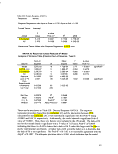 provides adequate signal strength. The assumptions and influence were investigated using
the diagnostic and influence plots discussed below.
First, normality is tested as shown in Figure 20, Density Response Diagnostic Plots.
A)
11 02267
0932
I
-2.68
B)
• m •
: * -iftJJ : • ':•
• .?«.': •
11.02267
0.982
I
0.994
C).
D)
I
1.01
Figure 20. Density Response Diagnostic Plots A) Normal Plot of Internally Studentized Residuals, B)
Internally Studentized Residuals vs. Predicted, C) Internally Studentized Residuals vs. Run, D) Predicted vs.
Actual
The Normal Plot of Residuals (Fig. 20 A) proves normality is achieved as the data points
primarily align along the straight line. The Residual vs. Predicted plot (Fig. 20B) shows a
good random scatter of points throughout the plotting space, with a possible outlier in the
lower right corner of the plot. The Residual vs. Run Plot (Fig. 20C) also shows a good
random scatter with no trends or run bias observed, and showing the outlier possibility as in
Fig. 20B. Finally, the Predicted vs. Actual plot (Fig. 20D) shows good prediction as the
points are evenly distributed about the 45° line.
44
image:
provides adequate signal strength. The assumptions and influence were investigated using
the diagnostic and influence plots discussed below.
First, normality is tested as shown in Figure 20, Density Response Diagnostic Plots.
A)
11 02267
0932
I
-2.68
B)
• m •
: * -iftJJ : • ':•
• .?«.': •
11.02267
0.982
I
0.994
C).
D)
I
1.01
Figure 20. Density Response Diagnostic Plots A) Normal Plot of Internally Studentized Residuals, B)
Internally Studentized Residuals vs. Predicted, C) Internally Studentized Residuals vs. Run, D) Predicted vs.
Actual
The Normal Plot of Residuals (Fig. 20 A) proves normality is achieved as the data points
primarily align along the straight line. The Residual vs. Predicted plot (Fig. 20B) shows a
good random scatter of points throughout the plotting space, with a possible outlier in the
lower right corner of the plot. The Residual vs. Run Plot (Fig. 20C) also shows a good
random scatter with no trends or run bias observed, and showing the outlier possibility as in
Fig. 20B. Finally, the Predicted vs. Actual plot (Fig. 20D) shows good prediction as the
points are evenly distributed about the 45° line.
44
image:
 A)
• 1.0226)
• 0.982
C)
• 1.02267
10.903
0 33 67 100 133 167 200
PCEOORC
i
1.15 -
•0.70 -
-2.56 -
K. 02267
.982
-4.41 -
1
1
1
1
1
1 1
1
a
1
1
1
1
a
1
1
1
1
1
1
•
;• iiiv.il
I'll!
ritmtn
• • •
• •
123496769 10
Figure 21, Density Response Residuals vs.
Factors includes the plots of the residuals per
each factor, PCE concentration (Fig. 21 A),
Dye (Fig. 2IB), and Surfactant (Fig. 21C).
Each of these plots shows no clear bias or
increase of points above or below the zero-
line at either end of the range. Therefore,
there are no obvious grouping of effects
based on these plots.
Figure 21. Density Response Residual vs. Factors A)
Internally Studentized Residuals vs. PCE
concentration, B) Internally Studentized Residuals
vs. Dye, C) Internally Studentized Residuals vs.
Surfactant
45
image:
A)
• 1.0226)
• 0.982
C)
• 1.02267
10.903
0 33 67 100 133 167 200
PCEOORC
i
1.15 -
•0.70 -
-2.56 -
K. 02267
.982
-4.41 -
1
1
1
1
1
1 1
1
a
1
1
1
1
a
1
1
1
1
1
1
•
;• iiiv.il
I'll!
ritmtn
• • •
• •
123496769 10
Figure 21, Density Response Residuals vs.
Factors includes the plots of the residuals per
each factor, PCE concentration (Fig. 21 A),
Dye (Fig. 2IB), and Surfactant (Fig. 21C).
Each of these plots shows no clear bias or
increase of points above or below the zero-
line at either end of the range. Therefore,
there are no obvious grouping of effects
based on these plots.
Figure 21. Density Response Residual vs. Factors A)
Internally Studentized Residuals vs. PCE
concentration, B) Internally Studentized Residuals
vs. Dye, C) Internally Studentized Residuals vs.
Surfactant
45
image:
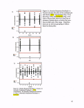 The influence plots were inspected for the possibility of outliers or the presence of
influential runs. These plots are shown in Figure 22, Density Response Influence Plots.
A)
B)
C)
11.02267
0.982
D)
11.02267
0.982
RunNumtw RunNurtar
Figure 22. Density Response Influence Plots A) Externally Studentized Residuals, B) DFFITS vs. Run, C)
Leverage vs. Run, D) Cook's Distance
The Externally Studentized Residual plot (Fig. 22A) suggests one point outside the 95%
confidence limits (upper and lower horizontal red lines) located in the lower right corner of
the plot. The DFFITS (difference in fits) vs. Run plot (Fig. 22B) does not imply any overly
influential runs, as all points are well within +/-2.0. The Leverage vs. Run plot (Fig. 22C)
shows that all values plot along the average leverage, suggesting that no runs unduly
influence the model parameters. Finally, the Cook's Distance plot (Fig. 22D) does not
show any outliers. The possible outlier in Fig. 22A is not supported by the other density
influence plots and there is no experimental reason to consider this point an outlier. Thus
all data points are included in the density response analysis.
46
image:
The influence plots were inspected for the possibility of outliers or the presence of
influential runs. These plots are shown in Figure 22, Density Response Influence Plots.
A)
B)
C)
11.02267
0.982
D)
11.02267
0.982
RunNumtw RunNurtar
Figure 22. Density Response Influence Plots A) Externally Studentized Residuals, B) DFFITS vs. Run, C)
Leverage vs. Run, D) Cook's Distance
The Externally Studentized Residual plot (Fig. 22A) suggests one point outside the 95%
confidence limits (upper and lower horizontal red lines) located in the lower right corner of
the plot. The DFFITS (difference in fits) vs. Run plot (Fig. 22B) does not imply any overly
influential runs, as all points are well within +/-2.0. The Leverage vs. Run plot (Fig. 22C)
shows that all values plot along the average leverage, suggesting that no runs unduly
influence the model parameters. Finally, the Cook's Distance plot (Fig. 22D) does not
show any outliers. The possible outlier in Fig. 22A is not supported by the other density
influence plots and there is no experimental reason to consider this point an outlier. Thus
all data points are included in the density response analysis.
46
image:
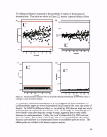 1.024 —
• C1 4%Tween80
A C2 4% Tween 80 + 10% EtOH
» C3 50 mM Tween 60
+ C4 0.5% AMA-80-1
X C58% AMA-80-1
M C6 0.025% Steol CS-330
¥ C70.1% Steol CS-330
• C8 0 5-< D'.i-Afax i • >
A C95%Dowfax8390
» C10 No Surfactant »
X1=A:PCEconc
X2 = C: Surfactant
Actual Factor
B: Dye = none
1.0135 —
0.9925 —
0.932 —
C: Surfactant
0.00
50.00
100.00
A: PCE cone
150.00
200.00
Figure 23. Density Response Plot showing the interaction of PCE concentration and Surfactant type.
The Density Model Response Plot is shown in Figure 23. This plot shows the
interaction of PCE concentration and surfactant type with no dye, because dye type is not a
significant factor. This plot shows the density value per each surfactant across the full
range of PCE concentration used. The density values are variable per the surfactant type;
however, an important note is the range of density values. These values range from a
maximum of 1.01123 to a minimum of 0.99376, which is a range of 0.01747. This
represents a very small dynamic range of the density response, which is not within the error
of the instrument measurement.
47
image:
1.024 —
• C1 4%Tween80
A C2 4% Tween 80 + 10% EtOH
» C3 50 mM Tween 60
+ C4 0.5% AMA-80-1
X C58% AMA-80-1
M C6 0.025% Steol CS-330
¥ C70.1% Steol CS-330
• C8 0 5-< D'.i-Afax i • >
A C95%Dowfax8390
» C10 No Surfactant »
X1=A:PCEconc
X2 = C: Surfactant
Actual Factor
B: Dye = none
1.0135 —
0.9925 —
0.932 —
C: Surfactant
0.00
50.00
100.00
A: PCE cone
150.00
200.00
Figure 23. Density Response Plot showing the interaction of PCE concentration and Surfactant type.
The Density Model Response Plot is shown in Figure 23. This plot shows the
interaction of PCE concentration and surfactant type with no dye, because dye type is not a
significant factor. This plot shows the density value per each surfactant across the full
range of PCE concentration used. The density values are variable per the surfactant type;
however, an important note is the range of density values. These values range from a
maximum of 1.01123 to a minimum of 0.99376, which is a range of 0.01747. This
represents a very small dynamic range of the density response, which is not within the error
of the instrument measurement.
47
image:
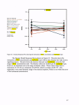 The Final Equation in Terms of Coded Factors (A: PCE cone., C: surfactant type)
for the density response is:
density =
+1.00
-3.807E-005 * A
+4.864E-004 * C[l]
-3.264E-003 * C[2]
+3.208E-003 * C[3]
-2.167E-003*C[4]
+7.765E-003 * C[5]
-1.652E-003 * C[6]
-1.376E-003*C[7]
-2.375E-003 * C[8]
+4.058E-005 * C[9]
-7.267E-004*AC[1]
+3.940E-003 * AC[2]
-8.019E-004 * AC[3]
-6.753E-003 * AC[4]
-7.016E-004*AC[5]
+1.631E-003*AC[6]
+9.259E-004 * AC[7]
-1.597E-004*AC[8]
+1.287E-003*AC[9]
48
image:
The Final Equation in Terms of Coded Factors (A: PCE cone., C: surfactant type)
for the density response is:
density =
+1.00
-3.807E-005 * A
+4.864E-004 * C[l]
-3.264E-003 * C[2]
+3.208E-003 * C[3]
-2.167E-003*C[4]
+7.765E-003 * C[5]
-1.652E-003 * C[6]
-1.376E-003*C[7]
-2.375E-003 * C[8]
+4.058E-005 * C[9]
-7.267E-004*AC[1]
+3.940E-003 * AC[2]
-8.019E-004 * AC[3]
-6.753E-003 * AC[4]
-7.016E-004*AC[5]
+1.631E-003*AC[6]
+9.259E-004 * AC[7]
-1.597E-004*AC[8]
+1.287E-003*AC[9]
48
image:
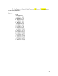 With the following error analysis:
Term
Intercept
A-PCE
cone
C[1]
C[2]
C[3]
C[4]
C[5]
C[6]
cm
C[8]
C[9]
AC[1]
AC[2]
AC[3]
AC[4]
AC[5]
AC[6]
AC[7]
AC[8]
AC[9]
Coefficient
Estimate
1 .002722
-3.8E-05
0.000486
-0.00326
0.003208
-0.00217
0.007765
-0.00165
-0.00138
-0.00237
4.06E-05
-0.00073
0.00394
-0.0008
-0.00675
-0.0007
0.001631
0.000926
-0.00016
0.001287
df
1
1
1
1
1
1
1
1
1
1
1
1
1
1
1
1
1
1
1
1
Standard
Error
0.000436
0.000581
0.001307
0.001307
0.001307
0.001307
0.001307
0.001307
0.001307
0.001307
0.001307
0.001743
0.001743
0.001743
0.001743
0.001743
0.001743
0.001743
0.001743
0.001743
95% Cl
Low
1.001863
-0.00118
-0.00209
-0.00584
0.000632
-0.00474
0.005188
-0.00423
-0.00395
-0.00495
-0.00254
-0.00416
0.000504
-0.00424
-0.01019
-0.00414
-0.0018
-0.00251
-0.0036
-0.00215
95% Cl
High
1.003581
0.001107
0.003063
-0.00069
0.005785
0.00041
0:010341
0.000925
0.001201
0.000202
0.002617
0.002709
0.007375
0.002634
-0.00332
0.002734
0.005067
0.004361
0.003276
0.004722
VIF
1
49
image:
With the following error analysis:
Term
Intercept
A-PCE
cone
C[1]
C[2]
C[3]
C[4]
C[5]
C[6]
cm
C[8]
C[9]
AC[1]
AC[2]
AC[3]
AC[4]
AC[5]
AC[6]
AC[7]
AC[8]
AC[9]
Coefficient
Estimate
1 .002722
-3.8E-05
0.000486
-0.00326
0.003208
-0.00217
0.007765
-0.00165
-0.00138
-0.00237
4.06E-05
-0.00073
0.00394
-0.0008
-0.00675
-0.0007
0.001631
0.000926
-0.00016
0.001287
df
1
1
1
1
1
1
1
1
1
1
1
1
1
1
1
1
1
1
1
1
Standard
Error
0.000436
0.000581
0.001307
0.001307
0.001307
0.001307
0.001307
0.001307
0.001307
0.001307
0.001307
0.001743
0.001743
0.001743
0.001743
0.001743
0.001743
0.001743
0.001743
0.001743
95% Cl
Low
1.001863
-0.00118
-0.00209
-0.00584
0.000632
-0.00474
0.005188
-0.00423
-0.00395
-0.00495
-0.00254
-0.00416
0.000504
-0.00424
-0.01019
-0.00414
-0.0018
-0.00251
-0.0036
-0.00215
95% Cl
High
1.003581
0.001107
0.003063
-0.00069
0.005785
0.00041
0:010341
0.000925
0.001201
0.000202
0.002617
0.002709
0.007375
0.002634
-0.00332
0.002734
0.005067
0.004361
0.003276
0.004722
VIF
1
49
image:
 3.7 Response Summary
A summary of the model responses is provided in Table XIII, Model Results
Summary.
Table X11I. Model Results Summary
Response
Temperature
PH'
Conductivity
DO
density
Transform
none
none
power,
A=0.5
power,
A=2.2
none
Model
linear
linear
linear
linear
2FI
Coded
Factors
B,C
C
B,C
A,B,C
C,AC
Adj. R2
0.0519
0.8199
0.9965
0.7801
0.1807
Pred. R2
-0.0022f
0.8112
0.9963
0.7666
0.1162
Model
Prob>F
0.0158
<0.0001
0.0001
O.0001
O.0001
LOF
Prob>F
0.3250
0.1986
0.9192
0.9307
0.0069
Tnegative Pred R* indicates that the Mean is a better predictor than the model using coded factors B
andC
* pH response is not normally distributed. Thus, pH may not be a predictable response
LOF = Lack-of-Fit
Coded Factors: A: PCE concentration; B: Dye type; C: Surfactant type
The table includes the response, if a transform was used, the model and coded terms, as
well as the relevant statistics for each response model. Of the predicable modeled
responses, conductivity shows the best model fit, followed by DO, and finally density. The
experimental factor levels which yield the highest and lowest experimental response values
are summarized in Table XIV, Maximum and Minimum Model Response Summary.
50
image:
3.7 Response Summary
A summary of the model responses is provided in Table XIII, Model Results
Summary.
Table X11I. Model Results Summary
Response
Temperature
PH'
Conductivity
DO
density
Transform
none
none
power,
A=0.5
power,
A=2.2
none
Model
linear
linear
linear
linear
2FI
Coded
Factors
B,C
C
B,C
A,B,C
C,AC
Adj. R2
0.0519
0.8199
0.9965
0.7801
0.1807
Pred. R2
-0.0022f
0.8112
0.9963
0.7666
0.1162
Model
Prob>F
0.0158
<0.0001
0.0001
O.0001
O.0001
LOF
Prob>F
0.3250
0.1986
0.9192
0.9307
0.0069
Tnegative Pred R* indicates that the Mean is a better predictor than the model using coded factors B
andC
* pH response is not normally distributed. Thus, pH may not be a predictable response
LOF = Lack-of-Fit
Coded Factors: A: PCE concentration; B: Dye type; C: Surfactant type
The table includes the response, if a transform was used, the model and coded terms, as
well as the relevant statistics for each response model. Of the predicable modeled
responses, conductivity shows the best model fit, followed by DO, and finally density. The
experimental factor levels which yield the highest and lowest experimental response values
are summarized in Table XIV, Maximum and Minimum Model Response Summary.
50
image:
 Table XIV: Maximum and Minimum Experimental Factor Levels Summary
Response
Temperature
pH
Conductivity
DO
density
maximum
minimum
maximum
minimum
maximum
minimum
maximum
minimum
maximum
minimum
Value
21.7°C
15.9°C
7.96
4.32
7610 |jS/cm
0.968 MS /cm
10.48mg/L
3.18mg/L
1 .023 g/mL
0.982 g/mL
Experimental Factor Level
(0.025% Steol CS-330)+ Oil-Red-O @ 200 ppm PCE
(4% Tween 80 + 10% EtOH) + No Dye @ 50 ppm PCE
5% Dowfax 8390 + Oil-Red-O @ 0 ppm PCE
(4% Tween 80 + 10% EtOH) + No Dye @ 150 ppm PCE
(8% AMA-80-I) + Oil-Red-O @ 100 ppm PCE
No surfactant + Oil-Red-O @ 200 ppm PCE
0.5 % Dowfax 8390 + Oil-Red-O @ 0 ppm PCE
4% Tween 80 + No Dye @ 200 ppm PCE
8% AMA-80-I + B.B. @ 1 50 ppm PCE
(0.5 % AMA-80-I ) + Oil-Red-O @ 200 ppm PCE
The temperature experimental results range from 21.7°C for (0.025% Steol CS-330)+ Oil-
Red-O @ 200 ppm PCE to 15.9°C for (4% Tween 80 + 10% EtOH) + No Dye @ 50 ppm
PCE. Experimentally we see a 5.8°C range; however, it is important to the note the model
results did no provide a statistically robust model and the mean of these experimental
results is quite possible a better predictor of the temperature response. The experimental
response for the pH reveals a range from 7.96 for 5% Dowfax 8390 + Oil-Red-O @ 0 ppm
PCE to 4.32 for (4% Tween 80 + 10% EtOH) + No Dye @ 150 ppm PCE. The total range
of pH is 3.64. The range of conductivity is quite large indicating the experimental
treatments have a profound effect on the conductivity of the aqueous solution. The
conductivity data range from 7610 to 0.968 uS/cm, with the 8% AMA-80-I + Oil-Red-O @
100 ppm having the highest conductivity and no surfactant + Oil-Red-O @ 200 ppm PCE
having the lowest conductivity. Because no PCE concentrations exceeded the solubility of
PCE at 20°C of 200 ppm, the 4-cell conductivity probe was used with the Denver
Instruments meter. Had free phase PCE been encountered the 2-cell probe would have
been used. This instrument has a conductivity accuracy of ±0.5% or ±0.01 uS/cm, which is
within the response summary for the conductivity response. Clearly, the specific
formulation of surfactant determines the conductivity of the aqueous solution. The
dissolved oxygen model response summary (Table XIV) shows a maximum of 10.48 mg/L
for the 0.5% Dowfax 8390 + Oil-Red-O and 0 ppm PCE and a minimum of 3.18 mg/L for
the 4% Tween 80 + No Dye at 200 ppm PCE. This range of DO values is within the
accuracy of the measuring instrument. The Accumet® AR60 used for the DO
measurements has an accuracy of ±0.1%. Finally, the density experimental results show a
range from 1.023 g/mL for 8 % AMA-80-I + B.B. @ 150 ppm PCE and 0.982 g/mL for
(0.5 % AMA-80-I) + Oil-Red-O @ 200 ppm PCE. This small range of 0.041 g/mL is not
within the practicality of the measurement method for this response. The density was
calculated from volume and mass measurements. Neither the volume nor the mass
measurements are within an accuracy of 0.041 g/mL. Therefore, density is not considered
a predictable response. Furthermore, since the temperature response yielded a statistically
weak model which suggests the mean as a better predictor and the pH experimental levels
were not normally distributed, only conductivity and dissolved oxygen were modeled with
practical significance.
51
image:
Table XIV: Maximum and Minimum Experimental Factor Levels Summary
Response
Temperature
pH
Conductivity
DO
density
maximum
minimum
maximum
minimum
maximum
minimum
maximum
minimum
maximum
minimum
Value
21.7°C
15.9°C
7.96
4.32
7610 |jS/cm
0.968 MS /cm
10.48mg/L
3.18mg/L
1 .023 g/mL
0.982 g/mL
Experimental Factor Level
(0.025% Steol CS-330)+ Oil-Red-O @ 200 ppm PCE
(4% Tween 80 + 10% EtOH) + No Dye @ 50 ppm PCE
5% Dowfax 8390 + Oil-Red-O @ 0 ppm PCE
(4% Tween 80 + 10% EtOH) + No Dye @ 150 ppm PCE
(8% AMA-80-I) + Oil-Red-O @ 100 ppm PCE
No surfactant + Oil-Red-O @ 200 ppm PCE
0.5 % Dowfax 8390 + Oil-Red-O @ 0 ppm PCE
4% Tween 80 + No Dye @ 200 ppm PCE
8% AMA-80-I + B.B. @ 1 50 ppm PCE
(0.5 % AMA-80-I ) + Oil-Red-O @ 200 ppm PCE
The temperature experimental results range from 21.7°C for (0.025% Steol CS-330)+ Oil-
Red-O @ 200 ppm PCE to 15.9°C for (4% Tween 80 + 10% EtOH) + No Dye @ 50 ppm
PCE. Experimentally we see a 5.8°C range; however, it is important to the note the model
results did no provide a statistically robust model and the mean of these experimental
results is quite possible a better predictor of the temperature response. The experimental
response for the pH reveals a range from 7.96 for 5% Dowfax 8390 + Oil-Red-O @ 0 ppm
PCE to 4.32 for (4% Tween 80 + 10% EtOH) + No Dye @ 150 ppm PCE. The total range
of pH is 3.64. The range of conductivity is quite large indicating the experimental
treatments have a profound effect on the conductivity of the aqueous solution. The
conductivity data range from 7610 to 0.968 uS/cm, with the 8% AMA-80-I + Oil-Red-O @
100 ppm having the highest conductivity and no surfactant + Oil-Red-O @ 200 ppm PCE
having the lowest conductivity. Because no PCE concentrations exceeded the solubility of
PCE at 20°C of 200 ppm, the 4-cell conductivity probe was used with the Denver
Instruments meter. Had free phase PCE been encountered the 2-cell probe would have
been used. This instrument has a conductivity accuracy of ±0.5% or ±0.01 uS/cm, which is
within the response summary for the conductivity response. Clearly, the specific
formulation of surfactant determines the conductivity of the aqueous solution. The
dissolved oxygen model response summary (Table XIV) shows a maximum of 10.48 mg/L
for the 0.5% Dowfax 8390 + Oil-Red-O and 0 ppm PCE and a minimum of 3.18 mg/L for
the 4% Tween 80 + No Dye at 200 ppm PCE. This range of DO values is within the
accuracy of the measuring instrument. The Accumet® AR60 used for the DO
measurements has an accuracy of ±0.1%. Finally, the density experimental results show a
range from 1.023 g/mL for 8 % AMA-80-I + B.B. @ 150 ppm PCE and 0.982 g/mL for
(0.5 % AMA-80-I) + Oil-Red-O @ 200 ppm PCE. This small range of 0.041 g/mL is not
within the practicality of the measurement method for this response. The density was
calculated from volume and mass measurements. Neither the volume nor the mass
measurements are within an accuracy of 0.041 g/mL. Therefore, density is not considered
a predictable response. Furthermore, since the temperature response yielded a statistically
weak model which suggests the mean as a better predictor and the pH experimental levels
were not normally distributed, only conductivity and dissolved oxygen were modeled with
practical significance.
51
image:
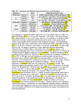 The experimental treatments are arranged in Table XV, Conductivity Model
Response in Ascending Order, for both the transformed and untransformed conductivity
response.
Table XV: Conductivity Model Response in Ascending Order
Experimental Treatment
No Surfactant + Oil-Red-O
No Surfactant + no dye
No Surfactant + Brilliant Blue
0.025% Steol CS-330 + Oil-Red-O
0.025% Steol CS-330 + no dye
4% Tween 80 + 10% EtOH + Oil-Red-O
0.025% Steol CS-330 + Brilliant Blue
4% Tween 80+10% EtOH + no dye
4% Tween 80+10% EtOH + Brilliant Blue
4% Tween 80 + Oil-Red-O
4% Tween 80 + no dye
4% Tween 80 + Brilliant Blue
0.1% Steol CS-330 + Oil-Red-O
0.1% Steol CS-330 + no dye
0. 1 % Steol CS-330 + Brilliant Blue
50 mM Tween 60 + Oil-Red-O
50 mM Tween 60 + no dye
50 mM Tween 60 + Brilliant Blue
0.5% Dowfax 8390 + Oil-Red-O
0.5% Dowfax 8390 + no dye
0.5% Dowfax 8390 + Brilliant Blue
0.5% AMA-80-1 + Oil-Red-O
0.5%AMA-80-I + no dye
0.5% AMA-80-1 + Brilliant Blue
5% Dowfax 8390 + Oil-Red-O
5% Dowfax 8390 + no dye
5% Dowfax 8390 + Brilliant Blue
8% AMA-80-1 + Oil-Red-O
8% AMA-80-1 + no dye
8% AMA-80-1 + Brilliant Blue
max
min
mean
stdev
condA0.5
1.74298
1.9828
2.97839
3.80387
4.0437
4.92205
5.03928
5.16187
6.15745
6.48027
6.72009
7.71568
7.81861
8.05843
9.05402
9.77533
10.0152
11.0107
19.9033
20.1431
21.1387
29.625
29.8648
30.8604
49.4176
49.6574
50.653
84.8056
85.045
86.041
86.041
1.74298
22.32118733
25.70229127
Cond (|jS/cm)
3.03797928
3.93149584
8.870806992
14.46942698
16.35150969
24.2265762
25.39434292
26.6449019
37.9141905
41.99389927
45.15960961
59.53171786
61.13066233
64.93829406
81.97527816
95.55707661
100.304231
121.2355145
396.1413509
405.7444776
446.8446377
877.640625
891.906279
952.3642882
2442.09919
2465.857375
2565.726409
7191.989791
7232.652025
7403.053681
7403.053681
3.03797928
1136.822921
2210.876587
52
image:
The experimental treatments are arranged in Table XV, Conductivity Model
Response in Ascending Order, for both the transformed and untransformed conductivity
response.
Table XV: Conductivity Model Response in Ascending Order
Experimental Treatment
No Surfactant + Oil-Red-O
No Surfactant + no dye
No Surfactant + Brilliant Blue
0.025% Steol CS-330 + Oil-Red-O
0.025% Steol CS-330 + no dye
4% Tween 80 + 10% EtOH + Oil-Red-O
0.025% Steol CS-330 + Brilliant Blue
4% Tween 80+10% EtOH + no dye
4% Tween 80+10% EtOH + Brilliant Blue
4% Tween 80 + Oil-Red-O
4% Tween 80 + no dye
4% Tween 80 + Brilliant Blue
0.1% Steol CS-330 + Oil-Red-O
0.1% Steol CS-330 + no dye
0. 1 % Steol CS-330 + Brilliant Blue
50 mM Tween 60 + Oil-Red-O
50 mM Tween 60 + no dye
50 mM Tween 60 + Brilliant Blue
0.5% Dowfax 8390 + Oil-Red-O
0.5% Dowfax 8390 + no dye
0.5% Dowfax 8390 + Brilliant Blue
0.5% AMA-80-1 + Oil-Red-O
0.5%AMA-80-I + no dye
0.5% AMA-80-1 + Brilliant Blue
5% Dowfax 8390 + Oil-Red-O
5% Dowfax 8390 + no dye
5% Dowfax 8390 + Brilliant Blue
8% AMA-80-1 + Oil-Red-O
8% AMA-80-1 + no dye
8% AMA-80-1 + Brilliant Blue
max
min
mean
stdev
condA0.5
1.74298
1.9828
2.97839
3.80387
4.0437
4.92205
5.03928
5.16187
6.15745
6.48027
6.72009
7.71568
7.81861
8.05843
9.05402
9.77533
10.0152
11.0107
19.9033
20.1431
21.1387
29.625
29.8648
30.8604
49.4176
49.6574
50.653
84.8056
85.045
86.041
86.041
1.74298
22.32118733
25.70229127
Cond (|jS/cm)
3.03797928
3.93149584
8.870806992
14.46942698
16.35150969
24.2265762
25.39434292
26.6449019
37.9141905
41.99389927
45.15960961
59.53171786
61.13066233
64.93829406
81.97527816
95.55707661
100.304231
121.2355145
396.1413509
405.7444776
446.8446377
877.640625
891.906279
952.3642882
2442.09919
2465.857375
2565.726409
7191.989791
7232.652025
7403.053681
7403.053681
3.03797928
1136.822921
2210.876587
52
image:
 This table organizes the conductivity response for quick inspection. Generally, the
conductivity increases per the type of surfactant, beginning with no surfactant as the least
conductive and ending with 8% AMA-80-I as the most conductive. The conductivity
ranking of dye type also shows a trend within each surfactant treatment. This may suggest
that the effect of the surfactant overwhelms the effect of the dye and any interaction
between surfactant and dye. The exception is with 4% Tween 80 + 10% EtOH + Oil-Red-
O and 0.025% Steol CS-330 + Brilliant Blue, the dye treatment is ordered from the least
conductive Oil-Red-0, no dye, to the most conductive Brilliant Blue G-250. This suggests
that Oil-Red-O results in an electrically resistive solution relative to the solution being
more conductive with no dye and most conductive with Brilliant Blue G-250. The least
electrically conductive surfactant treatment is no surfactant, while the most conductive is
the 8% AMA-80-I. The concentration of the particular surfactant does not necessarily
result in higher conductivity because 4% Tween 80 was found to be less conductive than
0.5% AMA-80-I. Rather, it seems that the conductivity is determined by the type of
surfactant and secondly by the dye type. The surfactant charge type does not present a
clear determination of the conductivity either. However, generally, the anionic types are
more conductive than the nonionic types.
53
image:
This table organizes the conductivity response for quick inspection. Generally, the
conductivity increases per the type of surfactant, beginning with no surfactant as the least
conductive and ending with 8% AMA-80-I as the most conductive. The conductivity
ranking of dye type also shows a trend within each surfactant treatment. This may suggest
that the effect of the surfactant overwhelms the effect of the dye and any interaction
between surfactant and dye. The exception is with 4% Tween 80 + 10% EtOH + Oil-Red-
O and 0.025% Steol CS-330 + Brilliant Blue, the dye treatment is ordered from the least
conductive Oil-Red-0, no dye, to the most conductive Brilliant Blue G-250. This suggests
that Oil-Red-O results in an electrically resistive solution relative to the solution being
more conductive with no dye and most conductive with Brilliant Blue G-250. The least
electrically conductive surfactant treatment is no surfactant, while the most conductive is
the 8% AMA-80-I. The concentration of the particular surfactant does not necessarily
result in higher conductivity because 4% Tween 80 was found to be less conductive than
0.5% AMA-80-I. Rather, it seems that the conductivity is determined by the type of
surfactant and secondly by the dye type. The surfactant charge type does not present a
clear determination of the conductivity either. However, generally, the anionic types are
more conductive than the nonionic types.
53
image:
 Table XVI: Dissolved Oxygen Model Response in Ascending Order
Experimental Treatment
4% Tween 80 + no dye
4% Tween 80 + Oil-Red-O
4% Tween 80 + Brilliant Blue
50 mM Tween 60 + no dye
50 mM Tween 60 + Oil-Red-O
4% Tween 80+10% EtOH + no dye
4% Tween 80 + 10% EtOH + Oil-Red-O
50 mM Tween 60 + Brilliant Blue
4% Tween 80 + 10% EtOH + Brilliant
Blue
No Surfactant + no dye
No Surfactant + Oil-Red-O
No Surfactant + Brilliant Blue
0.5%AMA-80-I + no dye
0.5% AMA-80-1 + Oil-Red-O
0.1% Steol CS-330 + no dye
0.025% Steol CS-330 + no dye
0.1% Steol CS-330 + Oil-Red-O
0.025% Steol CS-330 + Oil-Red-O
8%AMA-80-I + no dye
5% Dowfax 8390 + no dye
8% AMA-80-1 + Oil-Red-O
5% Dowfax 8390 + Oil-Red-O
0.5 % Dowfax 8390 + no dye
0.5% Dowfax 8390 + Oil-Red-O
0.5% AMA-80-1 + Brilliant Blue
0. 1% Steol CS-330 + Brilliant Blue
0.025% Steol CS-330 + Brilliant Blue
8% AMA-80-1 + Brilliant Blue
5% Dowfax 8390 + Brilliant Blue
0.5% Dowfax 8390 + Brilliant Blue
max
min
mean
st dev
DO @ 0 ppm
PCE
4.94068
5.06536
5.75028
6.25038
6.34498
6.67748
6.76497
6.88295
7.26621
7.65689
7.73128
8.16287
8.55997
8.62513
8.6943
8.70887
8.75826
8.77270
8.83927
8.85079
8.90198
8.91341
8.93534
8.99725
9.00622
9.13272
9.14645
9.26951
9.28040
9.36032
9.36032
4.94068
8.008240667
1.321257408
DO @ 100
ppm PCE
4.74765
4.87827
5.59050
6.10623
6.20347
6.54458
6.63417
6.75489
7.14636
7.54447
7.62017
8.05888
8.46182
8.52788
8.59798
8.61275
8.66280
8.67743
8.74487
8.75655
8.80839
8.81996
8.84217 ,
8.90486
8.91394
9.04199
9.05589
9.18040
9.19142
9.27225
9.27225
4.74765
7.896766333
1 .349488337
DO @ 200
ppm PCE
4.54472
4.68215
5.42504
5.95787
6.05797
6.40835
6.50020
6.62385
7.02405
7.43000
7.50709
7.95326
8.36228
8.42927
8.50036
8.51533
8.56606
8.58089
8.64923
8.66106
8.71359
8.72531
8.74781
8.81130
8.82050
8.95015
8.96422
9.09025
9.10139
9.18318
9.18318
4.54472
7.782891
1.379806523
Table XVI, Dissolved Oxygen Model Response in Ascending Order displays the
experimental treatments in ascending order of the DO response and sorted by increasing
concentration of PCE. This reveals a trend showing the DO to decrease with more PCE in
solution as indicated by the somewhat negative model parameter (-2.82) in the model for
factor A (see the final DO Equation in terms of Coded Factors). The ascending order of the
experimental treatments reveals no obvious trends. Generally, it can be seen that most of
the Brilliant Blue G-250 dye treatments occur with higher DO response; however, there are
exceptions to this generalization with 4% Tween 80 + Brilliant Blue, 50 mM Tween 60 +
Brilliant Blue, 4% Tween 80 + 10% EtOH + Brilliant Blue, and No surfactant + Brilliant
54
image:
Table XVI: Dissolved Oxygen Model Response in Ascending Order
Experimental Treatment
4% Tween 80 + no dye
4% Tween 80 + Oil-Red-O
4% Tween 80 + Brilliant Blue
50 mM Tween 60 + no dye
50 mM Tween 60 + Oil-Red-O
4% Tween 80+10% EtOH + no dye
4% Tween 80 + 10% EtOH + Oil-Red-O
50 mM Tween 60 + Brilliant Blue
4% Tween 80 + 10% EtOH + Brilliant
Blue
No Surfactant + no dye
No Surfactant + Oil-Red-O
No Surfactant + Brilliant Blue
0.5%AMA-80-I + no dye
0.5% AMA-80-1 + Oil-Red-O
0.1% Steol CS-330 + no dye
0.025% Steol CS-330 + no dye
0.1% Steol CS-330 + Oil-Red-O
0.025% Steol CS-330 + Oil-Red-O
8%AMA-80-I + no dye
5% Dowfax 8390 + no dye
8% AMA-80-1 + Oil-Red-O
5% Dowfax 8390 + Oil-Red-O
0.5 % Dowfax 8390 + no dye
0.5% Dowfax 8390 + Oil-Red-O
0.5% AMA-80-1 + Brilliant Blue
0. 1% Steol CS-330 + Brilliant Blue
0.025% Steol CS-330 + Brilliant Blue
8% AMA-80-1 + Brilliant Blue
5% Dowfax 8390 + Brilliant Blue
0.5% Dowfax 8390 + Brilliant Blue
max
min
mean
st dev
DO @ 0 ppm
PCE
4.94068
5.06536
5.75028
6.25038
6.34498
6.67748
6.76497
6.88295
7.26621
7.65689
7.73128
8.16287
8.55997
8.62513
8.6943
8.70887
8.75826
8.77270
8.83927
8.85079
8.90198
8.91341
8.93534
8.99725
9.00622
9.13272
9.14645
9.26951
9.28040
9.36032
9.36032
4.94068
8.008240667
1.321257408
DO @ 100
ppm PCE
4.74765
4.87827
5.59050
6.10623
6.20347
6.54458
6.63417
6.75489
7.14636
7.54447
7.62017
8.05888
8.46182
8.52788
8.59798
8.61275
8.66280
8.67743
8.74487
8.75655
8.80839
8.81996
8.84217 ,
8.90486
8.91394
9.04199
9.05589
9.18040
9.19142
9.27225
9.27225
4.74765
7.896766333
1 .349488337
DO @ 200
ppm PCE
4.54472
4.68215
5.42504
5.95787
6.05797
6.40835
6.50020
6.62385
7.02405
7.43000
7.50709
7.95326
8.36228
8.42927
8.50036
8.51533
8.56606
8.58089
8.64923
8.66106
8.71359
8.72531
8.74781
8.81130
8.82050
8.95015
8.96422
9.09025
9.10139
9.18318
9.18318
4.54472
7.782891
1.379806523
Table XVI, Dissolved Oxygen Model Response in Ascending Order displays the
experimental treatments in ascending order of the DO response and sorted by increasing
concentration of PCE. This reveals a trend showing the DO to decrease with more PCE in
solution as indicated by the somewhat negative model parameter (-2.82) in the model for
factor A (see the final DO Equation in terms of Coded Factors). The ascending order of the
experimental treatments reveals no obvious trends. Generally, it can be seen that most of
the Brilliant Blue G-250 dye treatments occur with higher DO response; however, there are
exceptions to this generalization with 4% Tween 80 + Brilliant Blue, 50 mM Tween 60 +
Brilliant Blue, 4% Tween 80 + 10% EtOH + Brilliant Blue, and No surfactant + Brilliant
54
image:
 Blue. It also appears that, generally, the Tween treatments resulted in low DO
concentrations, while the Dowfax, AMA-80-I and Steol CS-330 resulted in higher DO
values.
4.0 Discussion
Because only conductivity and DO yielded practically acceptable model responses,
these are the only responses considered predictable and merit further discussion.
4.1 Conductivity Response
In order to discuss the conductivity response, the experimental treatments were
inspected for their ionic type and compared to Table XV. With reference to the charge type
of the experimental factors (see Appendix K for Experimental Factor Properties), it appears
the majority of the anionic treatments have the highest conductivity while nonionic and a
few anionic treatments showed lower conductivities. Within the dye type treatment, Oil-
Red-0 (C2eH24N40) was the least conductive, no dye was next, and Brilliant Blue G-250
(C47H49N307S2Na) consistently showed the highest conductivity per dye type. Oil-Red-O
(see Appendix I for molecular structure) contains no free ions and is not a salt, as is
Brilliant Blue G-250. Oil-Red-O does contain a phenolic OH" group; however, at neutral
pH this is hydrogen bound and will not dissociate and result in an ionic form. Brilliant
Blue G-250 (see Appendix J for molecular structure), on the other hand, has two sulfonate
anions (SOs") and a sodium ion (Na+), aiding ionic dissolution. Therefore, due to the
molecular structure of these two dyes, it is clear that solutions containing Brilliant Blue G-
250 would result in higher conductivity and those with Oil-Red-O would show less
conductivity. Because water is a polar molecule, it is likely that experimental treatments
with no dye would be more conductive than the nonionic Oil-Red-O, and less conductive
than the charged salt, Brilliant Blue G-250.
The experimental conductivity responses were greater when surfactants were
included as an experimental treatment versus the lowest conductive responses when no
surfactant was used. The conductivity response from 8% AMA-80-I showed the highest
conductivity, which is perhaps due to the availability of the NaS group (see Appendix K)
and the relatively high concentration (8%) of this surfactant. The next lower conductivity
response was from the 5% Dowfax 8390. This is the second highest surfactant
concentration and the Dowfax 8390 is a disulfonate (see Appendix K) thereby possibly
increasing its ionic capacity. With lesser surfactant concentration, the 0.5% AMA-80-I was
more conductive than the 0.5% Dowfax, probably due to the NaS group being more ionic
or readily conductive than the disulfonate from the Dowfax. The Tween 60 exhibited the
next lower conductivity, which is perplexing since it is reported to be nonionic. The 0.1 %
Steol CS-330 was the next in decreasing conductivity, mostly due to its low concentration,
the sodium ion availability, and the anionic nature of the surfactant. Next, the 4% Tween
80 was shown to be more conductive than the 4% Tween 80 + EtOH and the 0.025% Steol.
The higher concentration of the Tween 80 probably explains the higher conductivity vs. the
0.025% Steol. Furthermore, the EtOH resulted in a lower conductivity because EtOH is
55
image:
Blue. It also appears that, generally, the Tween treatments resulted in low DO
concentrations, while the Dowfax, AMA-80-I and Steol CS-330 resulted in higher DO
values.
4.0 Discussion
Because only conductivity and DO yielded practically acceptable model responses,
these are the only responses considered predictable and merit further discussion.
4.1 Conductivity Response
In order to discuss the conductivity response, the experimental treatments were
inspected for their ionic type and compared to Table XV. With reference to the charge type
of the experimental factors (see Appendix K for Experimental Factor Properties), it appears
the majority of the anionic treatments have the highest conductivity while nonionic and a
few anionic treatments showed lower conductivities. Within the dye type treatment, Oil-
Red-0 (C2eH24N40) was the least conductive, no dye was next, and Brilliant Blue G-250
(C47H49N307S2Na) consistently showed the highest conductivity per dye type. Oil-Red-O
(see Appendix I for molecular structure) contains no free ions and is not a salt, as is
Brilliant Blue G-250. Oil-Red-O does contain a phenolic OH" group; however, at neutral
pH this is hydrogen bound and will not dissociate and result in an ionic form. Brilliant
Blue G-250 (see Appendix J for molecular structure), on the other hand, has two sulfonate
anions (SOs") and a sodium ion (Na+), aiding ionic dissolution. Therefore, due to the
molecular structure of these two dyes, it is clear that solutions containing Brilliant Blue G-
250 would result in higher conductivity and those with Oil-Red-O would show less
conductivity. Because water is a polar molecule, it is likely that experimental treatments
with no dye would be more conductive than the nonionic Oil-Red-O, and less conductive
than the charged salt, Brilliant Blue G-250.
The experimental conductivity responses were greater when surfactants were
included as an experimental treatment versus the lowest conductive responses when no
surfactant was used. The conductivity response from 8% AMA-80-I showed the highest
conductivity, which is perhaps due to the availability of the NaS group (see Appendix K)
and the relatively high concentration (8%) of this surfactant. The next lower conductivity
response was from the 5% Dowfax 8390. This is the second highest surfactant
concentration and the Dowfax 8390 is a disulfonate (see Appendix K) thereby possibly
increasing its ionic capacity. With lesser surfactant concentration, the 0.5% AMA-80-I was
more conductive than the 0.5% Dowfax, probably due to the NaS group being more ionic
or readily conductive than the disulfonate from the Dowfax. The Tween 60 exhibited the
next lower conductivity, which is perplexing since it is reported to be nonionic. The 0.1 %
Steol CS-330 was the next in decreasing conductivity, mostly due to its low concentration,
the sodium ion availability, and the anionic nature of the surfactant. Next, the 4% Tween
80 was shown to be more conductive than the 4% Tween 80 + EtOH and the 0.025% Steol.
The higher concentration of the Tween 80 probably explains the higher conductivity vs. the
0.025% Steol. Furthermore, the EtOH resulted in a lower conductivity because EtOH is
55
image:
 less conductive than water or, in other words, the ions dissolved in EtOH or in EtOH/water
are less conductive than in water (Wu and Berezansky, 1995).
Overall, the conductivity response was predictable per the model development
shown above. The relative conductivity response per experimental treatment is mostly
explained by the chemistry of each treatment.
4.2 Dissolved Oxygen Response
Dissolved oxygen analysis measures the amount of gaseous oxygen (02) dissolved
in an aqueous solution. The concentration of dissolved oxygen in water is affected by many
variables, such as ambient temperature, atmospheric pressure, and ion activity. Chemical
and biological reactions in ground water and surface water depend directly or indirectly on
the amount of available oxygen. Therefore, alterations in the concentration of DO in
groundwater due to the surfactant treatment of PCE are important to understand. To
discuss the DO results, the model responses are presented in Table XVI, Dissolved Oxygen
Model Response in Ascending Order. The table shows each experimental treatment at each
of the three PCE concentrations sorted by increasing DO model response. The results show
decreasing DO concentration with increasing PCE content. Generally, the Tween products
resulted in the lowest DO readings, while the Dowfax 8390 and AMA-80-I showed the
highest oxygen concentrations. For predictability purposes, each experimental treatment
would have to be entered into the DO model in order to predict the model DO response.
4.3 Implications to Geophysical Methods
This investigation into the physicochemical alterations of aqueous surfactants is a
first step to provide insight into the possibility of monitoring SEAR progress using
geophysical methods. The experiments accomplished this first step by producing
predictive models of the property changes occurring in an aqueous phase with various
remediation treatments. The implications of these results to the measurements made by
typical field geophysical methods are realized by investigating the liquid phase component
occupying the subsurface pore space during surfactant enhanced remediation.
Typical field geophysical methods can be categorized into magnetic, gravimetric,
seismic, and electrical methods. Unless the subsurface pore fluid contains ferrous materials
or binds ferrous materials onto soil or sediment grains, the traditional magnetic methods
will not detect changes in the chemistry of the pore fluid. Gravimetric methods measure
density contrasts in the subsurface. These methods can be applied with surface or borehole
measurements. Since the results from these experiments found the density response to vary
only ±0.02 mg/L, the gravity method is very unlikely to detect any changes within the
subsurface pore fluid.
56
image:
less conductive than water or, in other words, the ions dissolved in EtOH or in EtOH/water
are less conductive than in water (Wu and Berezansky, 1995).
Overall, the conductivity response was predictable per the model development
shown above. The relative conductivity response per experimental treatment is mostly
explained by the chemistry of each treatment.
4.2 Dissolved Oxygen Response
Dissolved oxygen analysis measures the amount of gaseous oxygen (02) dissolved
in an aqueous solution. The concentration of dissolved oxygen in water is affected by many
variables, such as ambient temperature, atmospheric pressure, and ion activity. Chemical
and biological reactions in ground water and surface water depend directly or indirectly on
the amount of available oxygen. Therefore, alterations in the concentration of DO in
groundwater due to the surfactant treatment of PCE are important to understand. To
discuss the DO results, the model responses are presented in Table XVI, Dissolved Oxygen
Model Response in Ascending Order. The table shows each experimental treatment at each
of the three PCE concentrations sorted by increasing DO model response. The results show
decreasing DO concentration with increasing PCE content. Generally, the Tween products
resulted in the lowest DO readings, while the Dowfax 8390 and AMA-80-I showed the
highest oxygen concentrations. For predictability purposes, each experimental treatment
would have to be entered into the DO model in order to predict the model DO response.
4.3 Implications to Geophysical Methods
This investigation into the physicochemical alterations of aqueous surfactants is a
first step to provide insight into the possibility of monitoring SEAR progress using
geophysical methods. The experiments accomplished this first step by producing
predictive models of the property changes occurring in an aqueous phase with various
remediation treatments. The implications of these results to the measurements made by
typical field geophysical methods are realized by investigating the liquid phase component
occupying the subsurface pore space during surfactant enhanced remediation.
Typical field geophysical methods can be categorized into magnetic, gravimetric,
seismic, and electrical methods. Unless the subsurface pore fluid contains ferrous materials
or binds ferrous materials onto soil or sediment grains, the traditional magnetic methods
will not detect changes in the chemistry of the pore fluid. Gravimetric methods measure
density contrasts in the subsurface. These methods can be applied with surface or borehole
measurements. Since the results from these experiments found the density response to vary
only ±0.02 mg/L, the gravity method is very unlikely to detect any changes within the
subsurface pore fluid.
56
image:
 Seismic methods generally measure the propagation of acoustic energy throughout the
subsurface. Principally, the p-wave and s-wave velocity are measured. These velocities
are shown below.
Where, Vp is the p-wave velocity and Vs the s-wave velocity. The variables K and u
represent the elastic and deformation behavior of the material through which the seismic
energy propagates. The density of the volume through which the seismic energy travels is
p. In a contaminated site, the solid materials within the subsurface remain relatively
unchanged, assuming negligible adsorption onto sediment particle or soil particles of a
particular contaminant or remediation fluid. This assumption is made to simplify this
discussion and relate it to this research. The interaction of the fluid with the solid portion
of the subsurface is very important in order to understand site dynamics and the
geophysical response. This is an area of consideration for future research. With this
assumption in place, the majority of change considered here in the subsurface is due to the
presence of the contaminated fluid (e.g., PCE) and a remediation method or treatment
component (e.g., a surfactant). So, the seismic method would predominately measure any
density changes within the pore fluid of the subsurface at a particular contaminated site.
The results from this experiment suggest that, in the case of PCE in its soluble form and the
surfactants studied, the density of the aqueous phase ranges from approximately 0.742 to
0.761 mg/L. Such a small dynamic range would most likely be undetectable using the
seismic method. Again, it is important to note that this statement is only based on the
experimental treatments used in this investigation and does not account for the effect of the
fluid-solid interface and any alterations which may occur from this interaction.
The implications of this study to electrical methods are next considered. The
conductivity model response yielded the largest dynamic range of the responses measured;
therefore, the conductivity of the aqueous solution was the most influenced by the
experimental treatments. All of the major geoelectrical methods either directly or
indirectly measure the conductivity of the fluid in the subsurface. In the direct current
(DC) resistivity method, Archie's Law (Archie, 1942) is the well established relationship
which explains the apparent resistivity or apparent conductivity of the subsurface. Archie's
Law is valid for geologic conditions in the absence of clays and is described by:
1
Where, ae is the effective conductivity of the medium, 0, the porosity, Sw, the water
saturation, 0Wi the pore water conductivity, m, the cementation exponent, n the saturation
exponent, and a is an empirical factor. The formation factor, F, includes the components
relevant to the solid portion of the subsurface. Without considering the effect and
interaction of the pore fluid on the solid portion of the medium, the effective conductivity
measured geophysically is directly proportional to the pore water conductivity. The
research presented herein addresses the pore water conductivity and has produced a
conductivity response model determined by the type of surfactant, dye, and concentration
57
image:
Seismic methods generally measure the propagation of acoustic energy throughout the
subsurface. Principally, the p-wave and s-wave velocity are measured. These velocities
are shown below.
Where, Vp is the p-wave velocity and Vs the s-wave velocity. The variables K and u
represent the elastic and deformation behavior of the material through which the seismic
energy propagates. The density of the volume through which the seismic energy travels is
p. In a contaminated site, the solid materials within the subsurface remain relatively
unchanged, assuming negligible adsorption onto sediment particle or soil particles of a
particular contaminant or remediation fluid. This assumption is made to simplify this
discussion and relate it to this research. The interaction of the fluid with the solid portion
of the subsurface is very important in order to understand site dynamics and the
geophysical response. This is an area of consideration for future research. With this
assumption in place, the majority of change considered here in the subsurface is due to the
presence of the contaminated fluid (e.g., PCE) and a remediation method or treatment
component (e.g., a surfactant). So, the seismic method would predominately measure any
density changes within the pore fluid of the subsurface at a particular contaminated site.
The results from this experiment suggest that, in the case of PCE in its soluble form and the
surfactants studied, the density of the aqueous phase ranges from approximately 0.742 to
0.761 mg/L. Such a small dynamic range would most likely be undetectable using the
seismic method. Again, it is important to note that this statement is only based on the
experimental treatments used in this investigation and does not account for the effect of the
fluid-solid interface and any alterations which may occur from this interaction.
The implications of this study to electrical methods are next considered. The
conductivity model response yielded the largest dynamic range of the responses measured;
therefore, the conductivity of the aqueous solution was the most influenced by the
experimental treatments. All of the major geoelectrical methods either directly or
indirectly measure the conductivity of the fluid in the subsurface. In the direct current
(DC) resistivity method, Archie's Law (Archie, 1942) is the well established relationship
which explains the apparent resistivity or apparent conductivity of the subsurface. Archie's
Law is valid for geologic conditions in the absence of clays and is described by:
1
Where, ae is the effective conductivity of the medium, 0, the porosity, Sw, the water
saturation, 0Wi the pore water conductivity, m, the cementation exponent, n the saturation
exponent, and a is an empirical factor. The formation factor, F, includes the components
relevant to the solid portion of the subsurface. Without considering the effect and
interaction of the pore fluid on the solid portion of the medium, the effective conductivity
measured geophysically is directly proportional to the pore water conductivity. The
research presented herein addresses the pore water conductivity and has produced a
conductivity response model determined by the type of surfactant, dye, and concentration
57
image:
 of PCE used. Therefore, these results are an initial step in understanding and predicting
geoelectrical responses found with surfactant enhanced aquifer remediation.
The relationship between the pore fluid electrolyte, the solid material, and the
effective or bulk geoelectrical measurement is further refined by introducing the concept pf
two independent conduction mechanisms acting in parallel (Waxman and Smits, 1968).
This is necessary because Archie's Law is only valid for one conducting phase distributed
within a non-conductive phase. The model developed by Waxman and Smits (1968)
incorporates one component consisting of the free electrolyte within the pore space and the
second from the conductance contribution of the cation exchange capacity of a clay solid
fraction of the subsurface volume. This expression, as shown below, relates the measured
conductivity (C0) to the electrolytic conductivity (Cw), the cation-exchange capacity or clay
conductivity (Ce) per unit volume of earth, and the formation factor (F ).
Therefore, Waxman and Smits (1968) include the additional conduction mechanism
attributed to the clay solid portion of the subsurface. From the conductivity model
developed in this study, Cw can be predicted. The component of the conductivity due to the
clay cation exchange may be altered by the presence of PCE, dye, or surfactant in the
subsurface; so, this component should be further investigated if this study is to be
applicable to subsurface conditions with considerable clay content. If there is no clay
present, then F* is essentially the formation factor, F, from Archie's Law, and Ce = 0.
Hence, it can be seen that in the absence of clays, Archie's Law is the appropriate model.
However, when another conducting phase is involved, the connectivity of the phases (i.e.,
Archie's cementation exponent, m, for one phase) needs inclusion. Mixings models are
utilized to account for this complexity and can include two exponents that describe the
connectivity of each of the two phases (Glover et al., 2000).
Implicitly, Archie's law and the Waxman-Smits equation assume that the
conductivity is a real valued constant. To describe the resistivity more completely, a
complex valued resistivity as a function of frequency would represent a more complete
generalized relationship between the transmitted current and the measured return voltage
during a geoelectrical investigation of the subsurface. Originally developed and applied to
minerals exploration, the induced polarization (IP) techniques are designed to directly
observe and interpret the complex resistivity as a function of frequency (Butler, 2005). The
complex resistivity (CR) method measures the broadband frequency dependence of the IP
energy storage mechanism (i.e., electrical impedance) in the subsurface. The low
frequency (0.01-1000 Hz) electrical properties are determined from measurements of the
resistivity magnitude, ]p\, and the phase shift, $ , between a measured voltage and a received
current. The complex conductivity, a = 1/p is: <7* = cr + icr , where the
real,<7 = |<r|cos0, and imaginary, cr = |<r sin^ , conductivities are frequency-dependent
(Kemna et al., 2004; Slater and Lesmes, 2002). This model adds to Archie's law, which
only accounts for the high frequency bulk or electrolytic conductivity. Complex
conductivity includes the second mode of conduction from the low frequency conductivity,
which is due to surface conduction, and the result of electrochemical polarization occurring
at grain-fluid interfaces. At low frequencies (<1000 Hz) the complex conductivity of the
sample is
58
image:
of PCE used. Therefore, these results are an initial step in understanding and predicting
geoelectrical responses found with surfactant enhanced aquifer remediation.
The relationship between the pore fluid electrolyte, the solid material, and the
effective or bulk geoelectrical measurement is further refined by introducing the concept pf
two independent conduction mechanisms acting in parallel (Waxman and Smits, 1968).
This is necessary because Archie's Law is only valid for one conducting phase distributed
within a non-conductive phase. The model developed by Waxman and Smits (1968)
incorporates one component consisting of the free electrolyte within the pore space and the
second from the conductance contribution of the cation exchange capacity of a clay solid
fraction of the subsurface volume. This expression, as shown below, relates the measured
conductivity (C0) to the electrolytic conductivity (Cw), the cation-exchange capacity or clay
conductivity (Ce) per unit volume of earth, and the formation factor (F ).
Therefore, Waxman and Smits (1968) include the additional conduction mechanism
attributed to the clay solid portion of the subsurface. From the conductivity model
developed in this study, Cw can be predicted. The component of the conductivity due to the
clay cation exchange may be altered by the presence of PCE, dye, or surfactant in the
subsurface; so, this component should be further investigated if this study is to be
applicable to subsurface conditions with considerable clay content. If there is no clay
present, then F* is essentially the formation factor, F, from Archie's Law, and Ce = 0.
Hence, it can be seen that in the absence of clays, Archie's Law is the appropriate model.
However, when another conducting phase is involved, the connectivity of the phases (i.e.,
Archie's cementation exponent, m, for one phase) needs inclusion. Mixings models are
utilized to account for this complexity and can include two exponents that describe the
connectivity of each of the two phases (Glover et al., 2000).
Implicitly, Archie's law and the Waxman-Smits equation assume that the
conductivity is a real valued constant. To describe the resistivity more completely, a
complex valued resistivity as a function of frequency would represent a more complete
generalized relationship between the transmitted current and the measured return voltage
during a geoelectrical investigation of the subsurface. Originally developed and applied to
minerals exploration, the induced polarization (IP) techniques are designed to directly
observe and interpret the complex resistivity as a function of frequency (Butler, 2005). The
complex resistivity (CR) method measures the broadband frequency dependence of the IP
energy storage mechanism (i.e., electrical impedance) in the subsurface. The low
frequency (0.01-1000 Hz) electrical properties are determined from measurements of the
resistivity magnitude, ]p\, and the phase shift, $ , between a measured voltage and a received
current. The complex conductivity, a = 1/p is: <7* = cr + icr , where the
real,<7 = |<r|cos0, and imaginary, cr = |<r sin^ , conductivities are frequency-dependent
(Kemna et al., 2004; Slater and Lesmes, 2002). This model adds to Archie's law, which
only accounts for the high frequency bulk or electrolytic conductivity. Complex
conductivity includes the second mode of conduction from the low frequency conductivity,
which is due to surface conduction, and the result of electrochemical polarization occurring
at grain-fluid interfaces. At low frequencies (<1000 Hz) the complex conductivity of the
sample is
58
image:
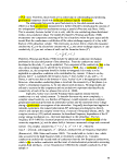 This model shows the real conductivity as the Archie's law conductivity due to electrolytic
conduction with the imaginary (i) conductivity due to surface conduction (aswf)
mechanisms as functions of the phase angle, co, between the transmitted current and the
voltage received (Lesmes and Frye, 2001). Therefore, this is a more general geoelectrical
model including the electrolytic and surface conduction. Again, the research shown in this
report provides a predictive conductivity model for the 0"w component of the complex
resistivity model relative to SEAR. Further research is needed to determine the surface
conduction component of the model due to PCE concentration, dye type, and surfactant
type.
Groundwater reactions result in small zones of distinctive water chemistry which
are the result of aerobic and anaerobic degradation of organic compounds and interactions
of the groundwater with the aquifer solids (Baedecker et al., 1993). Dissolved oxygen
levels can control microbial growth during which the carbon substrate is consumed,
nutrients are utilized, and byproducts are produced which alter the chemistry of the pore
fluid (Chapelle and Bradley, 1997) and the electrochemistry of the pore fluid.
Furthermore, the physical properties of the vadose, transition, and saturated zones may in
part be governed by the microbial ecology (Atekwana et al., 2006) which is, in turn,
governed by the aerobic conditions. Additionally, in groundwater the relationship between
the geophysical measurement of self-potential (SP) and redox conditions, which are
dependent on DO concentrations, has been demonstrated to alter the pore-fluid chemistry
(Naudt et al., 2003). Iron (II) oxidation through redox changes may also change the
surface conduction of a volume of the subsurface. The fact that.the subsurface
environment is altered physically, chemically, biologically, and geophysically by
groundwater reactions is well accepted; however, the mechanism or processes by which
these alterations occur is the subject of much research. The DO response model suggested
from this research furthers this area of investigation by predicting the DO response due to
PCE concentration, dye type, or surfactant type. It has been shown that DO governs
biological and chemical activity in the subsurface, thereby resulting in changes to the pore-
fluid chemistry and potentially changes in the geophysical measurements (Baedecker et al.,
1993; Bennett et al., 1993; Eganhouse et al., 1993). These changes in the geophysical
measurements due to the surfactant remediation of PCE are yet to be demonstrated.
Approximations to these changes can be seen through inspection of the geoelectrical
relationships noted above and the potential changes to the solid portions of the subsurface
through subsurface reactions and interactions. This research has shown that the DO
concentration does change due to the surfactant treatment of PCE. This change in the DO
level will impart geochemical and biological reactions in the subsurface which may be
detectable geophysically, either directly or indirectly. Future research should investigate
this possible link and the mechanism by which DO changes can alter the geophysical
response.
Overall, the application of this research to geophysical methods is predominately
relevant to geoelectrical methods. The conductivity response model shows the greatest
promise to utilize a predictive tool for geoelectrical methods. The DO response model does
show predictable and appreciable changes; however, the capacity of geophysical methods
to measure these changes is dependent upon the subsurface conditions, the geology, the
59
image:
This model shows the real conductivity as the Archie's law conductivity due to electrolytic
conduction with the imaginary (i) conductivity due to surface conduction (aswf)
mechanisms as functions of the phase angle, co, between the transmitted current and the
voltage received (Lesmes and Frye, 2001). Therefore, this is a more general geoelectrical
model including the electrolytic and surface conduction. Again, the research shown in this
report provides a predictive conductivity model for the 0"w component of the complex
resistivity model relative to SEAR. Further research is needed to determine the surface
conduction component of the model due to PCE concentration, dye type, and surfactant
type.
Groundwater reactions result in small zones of distinctive water chemistry which
are the result of aerobic and anaerobic degradation of organic compounds and interactions
of the groundwater with the aquifer solids (Baedecker et al., 1993). Dissolved oxygen
levels can control microbial growth during which the carbon substrate is consumed,
nutrients are utilized, and byproducts are produced which alter the chemistry of the pore
fluid (Chapelle and Bradley, 1997) and the electrochemistry of the pore fluid.
Furthermore, the physical properties of the vadose, transition, and saturated zones may in
part be governed by the microbial ecology (Atekwana et al., 2006) which is, in turn,
governed by the aerobic conditions. Additionally, in groundwater the relationship between
the geophysical measurement of self-potential (SP) and redox conditions, which are
dependent on DO concentrations, has been demonstrated to alter the pore-fluid chemistry
(Naudt et al., 2003). Iron (II) oxidation through redox changes may also change the
surface conduction of a volume of the subsurface. The fact that.the subsurface
environment is altered physically, chemically, biologically, and geophysically by
groundwater reactions is well accepted; however, the mechanism or processes by which
these alterations occur is the subject of much research. The DO response model suggested
from this research furthers this area of investigation by predicting the DO response due to
PCE concentration, dye type, or surfactant type. It has been shown that DO governs
biological and chemical activity in the subsurface, thereby resulting in changes to the pore-
fluid chemistry and potentially changes in the geophysical measurements (Baedecker et al.,
1993; Bennett et al., 1993; Eganhouse et al., 1993). These changes in the geophysical
measurements due to the surfactant remediation of PCE are yet to be demonstrated.
Approximations to these changes can be seen through inspection of the geoelectrical
relationships noted above and the potential changes to the solid portions of the subsurface
through subsurface reactions and interactions. This research has shown that the DO
concentration does change due to the surfactant treatment of PCE. This change in the DO
level will impart geochemical and biological reactions in the subsurface which may be
detectable geophysically, either directly or indirectly. Future research should investigate
this possible link and the mechanism by which DO changes can alter the geophysical
response.
Overall, the application of this research to geophysical methods is predominately
relevant to geoelectrical methods. The conductivity response model shows the greatest
promise to utilize a predictive tool for geoelectrical methods. The DO response model does
show predictable and appreciable changes; however, the capacity of geophysical methods
to measure these changes is dependent upon the subsurface conditions, the geology, the
59
image:
 hydrogeochemistry, and the interactions of these within the volume of earth measured. If
the DO changes produce appreciable variations to the geophysically relevant physical
properties in the subsurface, then geophysical methods may be applicable for monitoring.
The density changes which are documented in this research do not present a sufficiently
large change to measure geophysically. Depending on the type of surfactant used, the
geologic conditions, and the contaminant distribution at a site, it is very likely that a surface
geoelectrical method can measure the presence of the surfactant in the subsurface. The
results from this research demonstrate that electrolytic conduction is greatly changed by the
experimental treatments used.
5.0 Conclusions and Implications
This research provides initial models to predict aqueous property changes in SEAR
as applied to PCE through a RSM design of experiment. Experiments with 240 treatment
variations used PCE concentration as a numerical factor, and dye and surfactant type
nominal categorical factors and 5 responses: temperature, pH, conductivity, dissolved
oxygen, and density, were measured. The results found that the mean of the temperature
response proved a better predictor than the response model. The pH response was not
normally distributed and, therefore, not used in model development. Conductivity, DO,
and density responses yielded predictable response models; however, the range of the
density response was very small and did not exceed the tolerance of the measurement.
The conductivity response model is most relevant to geophysical measurements in
its ability to predict the pore water conductivity. The influence of pore water conductivity
was shown to be directly proportional to DC resistivity measurement, induced polarization,
and complex resistivity measurements. The DO model response is applicable to
geophysical measurements through its role in altering the pore water chemistry, biological
activity, and the interactions with the solid portions of the aquifer material. These
interactions were not investigated, but this research shows that SEAR of PCE results in
changes to the pore water, which quite probably can influence the interaction between the
pore water with the solid phases in the subsurface.
Of the experimental factors, dye type and surfactant type were the only factors to
significantly affect the conductivity response. The DO response was significantly
influenced by all three factors: PCE concentration, dye type, and surfactant type.
The results from this research provide predictive models of the conductivity and
dissolved oxygen, in the liquid phase, stemming from the surfactant remediation of PCE.
These models can be used to guide further studies of increasing complexity, including the
contribution of solid phases and the interaction of the solid and fluid components in the
geophysical response. These models will be applicable to monitoring and characterizing
field applications of SEAR at PCE contaminated sites. Depending on the geologic
conditions, this research has shown that the conductivity changes result in measurable
values attributable to the surfactant remediation of PCE. Furthermore, this research has
also shown that the use of Oil-Red-O or Brilliant Blue G-250 in visual tracer studies of
PCE migration will alter the aqueous properties of the pore water. This phenomenon
should be considered if these aqueous properties are of interest in the system under
investigation.
60
image:
hydrogeochemistry, and the interactions of these within the volume of earth measured. If
the DO changes produce appreciable variations to the geophysically relevant physical
properties in the subsurface, then geophysical methods may be applicable for monitoring.
The density changes which are documented in this research do not present a sufficiently
large change to measure geophysically. Depending on the type of surfactant used, the
geologic conditions, and the contaminant distribution at a site, it is very likely that a surface
geoelectrical method can measure the presence of the surfactant in the subsurface. The
results from this research demonstrate that electrolytic conduction is greatly changed by the
experimental treatments used.
5.0 Conclusions and Implications
This research provides initial models to predict aqueous property changes in SEAR
as applied to PCE through a RSM design of experiment. Experiments with 240 treatment
variations used PCE concentration as a numerical factor, and dye and surfactant type
nominal categorical factors and 5 responses: temperature, pH, conductivity, dissolved
oxygen, and density, were measured. The results found that the mean of the temperature
response proved a better predictor than the response model. The pH response was not
normally distributed and, therefore, not used in model development. Conductivity, DO,
and density responses yielded predictable response models; however, the range of the
density response was very small and did not exceed the tolerance of the measurement.
The conductivity response model is most relevant to geophysical measurements in
its ability to predict the pore water conductivity. The influence of pore water conductivity
was shown to be directly proportional to DC resistivity measurement, induced polarization,
and complex resistivity measurements. The DO model response is applicable to
geophysical measurements through its role in altering the pore water chemistry, biological
activity, and the interactions with the solid portions of the aquifer material. These
interactions were not investigated, but this research shows that SEAR of PCE results in
changes to the pore water, which quite probably can influence the interaction between the
pore water with the solid phases in the subsurface.
Of the experimental factors, dye type and surfactant type were the only factors to
significantly affect the conductivity response. The DO response was significantly
influenced by all three factors: PCE concentration, dye type, and surfactant type.
The results from this research provide predictive models of the conductivity and
dissolved oxygen, in the liquid phase, stemming from the surfactant remediation of PCE.
These models can be used to guide further studies of increasing complexity, including the
contribution of solid phases and the interaction of the solid and fluid components in the
geophysical response. These models will be applicable to monitoring and characterizing
field applications of SEAR at PCE contaminated sites. Depending on the geologic
conditions, this research has shown that the conductivity changes result in measurable
values attributable to the surfactant remediation of PCE. Furthermore, this research has
also shown that the use of Oil-Red-O or Brilliant Blue G-250 in visual tracer studies of
PCE migration will alter the aqueous properties of the pore water. This phenomenon
should be considered if these aqueous properties are of interest in the system under
investigation.
60
image:
 Finally, the research approach using RSM was a successful, albeit unconventional,
use of RSM design of experiments to create response models for pore fluid properties.
This powerful experimental design tool should be utilized for future investigations of
increased complexity to further this research topic. Future research should investigate
property changes due to other PCE remediation methods and combined remediation
methods, such as SEAR and the biologically mediated breakdown of PCE.
6.0 Acknowledgements
Many thanks are due to John Nocerino for his thorough, constructive comments and
suggestions regarding experimental design and the analysis portions of this study.
Furthermore, Daniel Chang provided exceptional comments which also made this report
stronger and more comprehensive. John Zimmerman served as an excellent technical
sounding board and critic as well as provided the GC/MS analysis and laboratory
functional support. Thanks to Vicki Ecker for performing the laboratory experiments and
her editing skills. Finally, thanks to Brian Schumacher for providing the laboratory space
and funding support to complete this work. Without the generous support from the above
individuals this work would not have been possible. For this I am gratefully appreciative.
61
image:
Finally, the research approach using RSM was a successful, albeit unconventional,
use of RSM design of experiments to create response models for pore fluid properties.
This powerful experimental design tool should be utilized for future investigations of
increased complexity to further this research topic. Future research should investigate
property changes due to other PCE remediation methods and combined remediation
methods, such as SEAR and the biologically mediated breakdown of PCE.
6.0 Acknowledgements
Many thanks are due to John Nocerino for his thorough, constructive comments and
suggestions regarding experimental design and the analysis portions of this study.
Furthermore, Daniel Chang provided exceptional comments which also made this report
stronger and more comprehensive. John Zimmerman served as an excellent technical
sounding board and critic as well as provided the GC/MS analysis and laboratory
functional support. Thanks to Vicki Ecker for performing the laboratory experiments and
her editing skills. Finally, thanks to Brian Schumacher for providing the laboratory space
and funding support to complete this work. Without the generous support from the above
individuals this work would not have been possible. For this I am gratefully appreciative.
61
image:
 7.0 References
References Cited
Anderson, M.J., Kraber, S., and Whitcomb, P.J., 2006, Handbook for Experimenters,
Minneapolis, MM, Stat-Ease, Inc., p. 1-31.
Anderson, M.J. and Whitcomb, P.J., 2005, RSM Simplified: Optimizing Processes Using
Response Surface Methods for Design of Experiments: New York, NY,
Productivity Press, p. 1 -292.
Anderson, M.J. and Whitcomb, P.J., 2000, DOE Simplified: Practical Tools for Effective
Experimentation: New York, NY, Productivity Press, p. 1-236.
Archie, G.E., 1942, The Electrical Resistivity Log as an Aid in Determining Some
Reservoir Characteristics, p. 54-62.
Atekwana, E.A., Werkema, D.D., and Atekwana, E.A., 2006, Biogeophysics: The effects
of microbial processes on geophysical properties of the shallow subsurface, in H.
Vereecken et al., ed., Applied Hydrogeophysics: Springer, p. 161-193.
Baedecker, M.J., Cozarelli, I.M., Eganhouse, R.P., Siegel, D.I., and Bennett, P.C., 1993,
Crude oil in a shallow sand and gravel aquifer: III. Biogeochemical reactions and
mass balance modeling in anoxic groundwater, p. 569-586.
Bennett, P.C., Siegel, D.I., Baedecker, M.J., and Hull, M.F., 1993, Crude oil in a shallow
sand and gravel aquifer: I. Hydrogeology and inorganic geochemistry, p. 529-549.
Box, G.E.P. and Cox, D.R., 1964, An analysis of transformations, p. 211-252.
Butler, D.K., 2005, Near-Surface Geophysics: Society of Exploration Geophysicists.
Chapelle, F.H. and Bradley, P.M., 1997, Alteration of aquifer geochemistry by
microorganisms, p. 558-564.
Cho, J., Annable, M.D., and Rao, P.S., 2004, Influence of residual surfactants on DNAPL
characterization using partitioning tracers: Journal of Contaminant Hydrology, v.
72, p. 67-83.
Conrad, S.H., Glass, R.J., and Peplinski, W.J., 2002, Bench-scale visualization of DNAPL
remediation processes in analog heterogeneous aquifers: surfactant floods and in
situ oxidation using permanganate: Journal of Contaminant Hydrology, v. 58, p. 13-
49.
62
image:
7.0 References
References Cited
Anderson, M.J., Kraber, S., and Whitcomb, P.J., 2006, Handbook for Experimenters,
Minneapolis, MM, Stat-Ease, Inc., p. 1-31.
Anderson, M.J. and Whitcomb, P.J., 2005, RSM Simplified: Optimizing Processes Using
Response Surface Methods for Design of Experiments: New York, NY,
Productivity Press, p. 1 -292.
Anderson, M.J. and Whitcomb, P.J., 2000, DOE Simplified: Practical Tools for Effective
Experimentation: New York, NY, Productivity Press, p. 1-236.
Archie, G.E., 1942, The Electrical Resistivity Log as an Aid in Determining Some
Reservoir Characteristics, p. 54-62.
Atekwana, E.A., Werkema, D.D., and Atekwana, E.A., 2006, Biogeophysics: The effects
of microbial processes on geophysical properties of the shallow subsurface, in H.
Vereecken et al., ed., Applied Hydrogeophysics: Springer, p. 161-193.
Baedecker, M.J., Cozarelli, I.M., Eganhouse, R.P., Siegel, D.I., and Bennett, P.C., 1993,
Crude oil in a shallow sand and gravel aquifer: III. Biogeochemical reactions and
mass balance modeling in anoxic groundwater, p. 569-586.
Bennett, P.C., Siegel, D.I., Baedecker, M.J., and Hull, M.F., 1993, Crude oil in a shallow
sand and gravel aquifer: I. Hydrogeology and inorganic geochemistry, p. 529-549.
Box, G.E.P. and Cox, D.R., 1964, An analysis of transformations, p. 211-252.
Butler, D.K., 2005, Near-Surface Geophysics: Society of Exploration Geophysicists.
Chapelle, F.H. and Bradley, P.M., 1997, Alteration of aquifer geochemistry by
microorganisms, p. 558-564.
Cho, J., Annable, M.D., and Rao, P.S., 2004, Influence of residual surfactants on DNAPL
characterization using partitioning tracers: Journal of Contaminant Hydrology, v.
72, p. 67-83.
Conrad, S.H., Glass, R.J., and Peplinski, W.J., 2002, Bench-scale visualization of DNAPL
remediation processes in analog heterogeneous aquifers: surfactant floods and in
situ oxidation using permanganate: Journal of Contaminant Hydrology, v. 58, p. 13-
49.
62
image:
 Denver Instrument Co., 1999, Denver Instrument Company Model 250
pH/Ion/Conductivity Meter Operation Manual: Denver Instrument Company.
Dwarakanath, V., Kostarelos, K., Pope, G.A., Shotts, D., and Wade, W.H., 1999, Anionic
surfactant remediation of soil columns contaminated by nonaqueous phase liquids:
Journal of Contaminant Hydrology, v. 38, p. 465-488.
Dwarakanath, V. and Pope, G.A., 2000, Surfactant Phase Behavior with Field Degreasing
Solvent, p. 4842-4848.
Eganhouse, R.P., Baedecker, M.J., Cozarelli, I.M., Aiken, G.R., Thorn, K.A., and Dorsey,
T.F., 1993, Crude oil in a shallow sand and gravel aquifer: II. Organic
geochemistry, p. 551-567.
Fisher Scientific, 2003, Accumet Research Model AR60 User Manual: Fisher Scientific.
Glover, P.W.J., Hole, M.J., and Pous, J., 2000, A modified Archie's law for two conducting
phases: Earth and Planetary Science Letters, v. 180, p. 369-383.
Jeong, S.W., Wood, A.L., and Lee, T.R., 2002, Effects of pure and dyed PCE on physical
and interfacial properties of remedial solutions: Journal of Hazardous Materials, v.
In Press, Corrected Proof.
Kemna, A., Binley, A., and Slater, L., 2004, Cross-borehole IP imaging for engineering and
environmental applications: Geophysics, v. 67, p. 97-107.
Kleinbaum, D.G., Kupper, L.L., Muller K.E., and Nizam, A., 1998, Applied Regression
Analysis and Multivariable Methods: Duxbury Press, p. 1-798.
Knight, R.J. and Endres, A.L., 2005, An introduction to rock physics principles for near-
surface geophysics, in Butler, D.K., ed., Near-Surface Geophysics: Society of
Exploration Geophysicists, p. 31 -70.
Lesmes, D.P. and Frye, K.M., 2001, Influence of pore fluid chemistry on the complex
conductivity and induced polarization responses of Berea sandstone, p. 4079-4090.
Londergan, J.T., Meinardus, H.W., Mariner, P.E., Jackson, R.E., Brown, C.L.,
Dwarakanath, V., Pope, G.A., Ginn, J.S., and Taffmder, S., 2001, DNAPL Removal
from a heterogeneous alluvial aquifer by surfactant-enhanced aquifer remediation,
p. 57-66.
Longino, B.L. and Kueper, B.H., 1994, The use of upward gradients to arrest downward
dense, nonaqueous phase liquid (DNAPL) migration in the presence of solubilizing
surfactants, p. 296-308.
McGuire, T. and Hughes, J.B., 2003, Effects of surfactants on the dechlorination of
chlorinated ethenes, p. 2630-2638.
63
image:
Denver Instrument Co., 1999, Denver Instrument Company Model 250
pH/Ion/Conductivity Meter Operation Manual: Denver Instrument Company.
Dwarakanath, V., Kostarelos, K., Pope, G.A., Shotts, D., and Wade, W.H., 1999, Anionic
surfactant remediation of soil columns contaminated by nonaqueous phase liquids:
Journal of Contaminant Hydrology, v. 38, p. 465-488.
Dwarakanath, V. and Pope, G.A., 2000, Surfactant Phase Behavior with Field Degreasing
Solvent, p. 4842-4848.
Eganhouse, R.P., Baedecker, M.J., Cozarelli, I.M., Aiken, G.R., Thorn, K.A., and Dorsey,
T.F., 1993, Crude oil in a shallow sand and gravel aquifer: II. Organic
geochemistry, p. 551-567.
Fisher Scientific, 2003, Accumet Research Model AR60 User Manual: Fisher Scientific.
Glover, P.W.J., Hole, M.J., and Pous, J., 2000, A modified Archie's law for two conducting
phases: Earth and Planetary Science Letters, v. 180, p. 369-383.
Jeong, S.W., Wood, A.L., and Lee, T.R., 2002, Effects of pure and dyed PCE on physical
and interfacial properties of remedial solutions: Journal of Hazardous Materials, v.
In Press, Corrected Proof.
Kemna, A., Binley, A., and Slater, L., 2004, Cross-borehole IP imaging for engineering and
environmental applications: Geophysics, v. 67, p. 97-107.
Kleinbaum, D.G., Kupper, L.L., Muller K.E., and Nizam, A., 1998, Applied Regression
Analysis and Multivariable Methods: Duxbury Press, p. 1-798.
Knight, R.J. and Endres, A.L., 2005, An introduction to rock physics principles for near-
surface geophysics, in Butler, D.K., ed., Near-Surface Geophysics: Society of
Exploration Geophysicists, p. 31 -70.
Lesmes, D.P. and Frye, K.M., 2001, Influence of pore fluid chemistry on the complex
conductivity and induced polarization responses of Berea sandstone, p. 4079-4090.
Londergan, J.T., Meinardus, H.W., Mariner, P.E., Jackson, R.E., Brown, C.L.,
Dwarakanath, V., Pope, G.A., Ginn, J.S., and Taffmder, S., 2001, DNAPL Removal
from a heterogeneous alluvial aquifer by surfactant-enhanced aquifer remediation,
p. 57-66.
Longino, B.L. and Kueper, B.H., 1994, The use of upward gradients to arrest downward
dense, nonaqueous phase liquid (DNAPL) migration in the presence of solubilizing
surfactants, p. 296-308.
McGuire, T. and Hughes, J.B., 2003, Effects of surfactants on the dechlorination of
chlorinated ethenes, p. 2630-2638.
63
image:
 Montgomery, D.C., 1997, Design and Analysis of Experiments: New York, NY, John
Wiley & Sons, Inc., p. 1-704.
Naudt, V., Revil, A., Bottero, J.Y., and Begassat, P., 2003, Relationship between self-
potential (SP) signals and redox conditions in contaminated groundwater, p. 2091.
NIOSH, 1994, NIOSH Pocket Guide to Chemical Hazards: U.S. Department of Health and
Human Services.
Pin-Hua, R., He, M., Xiao-Hui, M, Xian, Y., and Ming, Y., 2006, Effects of surfactants on
the stability of clay suspensions with special reference to the changes of pH: Soil
Science, v. 171, p. 764-771.
Ramsburg, C.A. and Pennell, K., 2000, Evaluation of surfactant formulations for treatment
of a PCE contaminated field site, in Wickramanayake, G.B., Gavaskar, A.R., and
Gupta, N., eds., Columbus, Battelle Press, p. 211-218.
Rommel, R.K., Peters, R.W., Martin, E.S., and Deflaun, M.F., 1998, Surfactant
foam/bioaugmentation technology for in situ treatment of TCE-DNAPLs, p. 1667-
1675.
Sabatini, D.A., Knox, R.C., and Harwell, J.H., 1995, Surfactant-Enhanced Subsurface
Remediation - Emerging Technologies: American Chemical Society.
Sabatini, D.A., Knox, R.C., and Harwell, J.H., 1996, Surfactant-Enhanced DNAPL
Remediation: surfactant selection, hydraulic efficiency, and economic factors, p. 1 -
14.
Sabatini, D.A., Knox, R.C., Harwell, J.H., and Wu, B., 2000, Integrated design of
surfactant enhanced DNAPL remediation: efficient supersolubilization and gradient
systems: Journal of Contaminant Hydrology, v. 45, p. 99-121.
Slater, L. and Lesmes, D.P., 2002, Electrical-hydraulic relationships observed for
unconsolidated sediments: Water Resources Research, v. 38, p. 31-1-31-12.
Stanely, T.W. and Verner, S.S., 1985, The U.S. Environmental Protection Agency's Quality
Assurance Program, Philadelphia, PA, American Society for Testing and Materials,
p. 12-19.
Stat-Ease, I., 2006, Design-Expert 7, www.statease.com.
Taylor, T.P., Pennell, K.D., Abriola, L.M., and Dane, J.H., 2001, Surfactant enhanced
recovery of tetrachloroethylene from a porous medium containing low permeability
lenses: 1. Experimental studies, p. 325-350.
Taylor, T.P., Rathfelder, K.M., Pennell, K.D., and Abriola, L.M., 2004, Effects of ethanol
addition on micellar solubilization and plume migration during surfactant enhanced
recovery of tetrachloroethene, p. 73-99.
64
image:
Montgomery, D.C., 1997, Design and Analysis of Experiments: New York, NY, John
Wiley & Sons, Inc., p. 1-704.
Naudt, V., Revil, A., Bottero, J.Y., and Begassat, P., 2003, Relationship between self-
potential (SP) signals and redox conditions in contaminated groundwater, p. 2091.
NIOSH, 1994, NIOSH Pocket Guide to Chemical Hazards: U.S. Department of Health and
Human Services.
Pin-Hua, R., He, M., Xiao-Hui, M, Xian, Y., and Ming, Y., 2006, Effects of surfactants on
the stability of clay suspensions with special reference to the changes of pH: Soil
Science, v. 171, p. 764-771.
Ramsburg, C.A. and Pennell, K., 2000, Evaluation of surfactant formulations for treatment
of a PCE contaminated field site, in Wickramanayake, G.B., Gavaskar, A.R., and
Gupta, N., eds., Columbus, Battelle Press, p. 211-218.
Rommel, R.K., Peters, R.W., Martin, E.S., and Deflaun, M.F., 1998, Surfactant
foam/bioaugmentation technology for in situ treatment of TCE-DNAPLs, p. 1667-
1675.
Sabatini, D.A., Knox, R.C., and Harwell, J.H., 1995, Surfactant-Enhanced Subsurface
Remediation - Emerging Technologies: American Chemical Society.
Sabatini, D.A., Knox, R.C., and Harwell, J.H., 1996, Surfactant-Enhanced DNAPL
Remediation: surfactant selection, hydraulic efficiency, and economic factors, p. 1 -
14.
Sabatini, D.A., Knox, R.C., Harwell, J.H., and Wu, B., 2000, Integrated design of
surfactant enhanced DNAPL remediation: efficient supersolubilization and gradient
systems: Journal of Contaminant Hydrology, v. 45, p. 99-121.
Slater, L. and Lesmes, D.P., 2002, Electrical-hydraulic relationships observed for
unconsolidated sediments: Water Resources Research, v. 38, p. 31-1-31-12.
Stanely, T.W. and Verner, S.S., 1985, The U.S. Environmental Protection Agency's Quality
Assurance Program, Philadelphia, PA, American Society for Testing and Materials,
p. 12-19.
Stat-Ease, I., 2006, Design-Expert 7, www.statease.com.
Taylor, T.P., Pennell, K.D., Abriola, L.M., and Dane, J.H., 2001, Surfactant enhanced
recovery of tetrachloroethylene from a porous medium containing low permeability
lenses: 1. Experimental studies, p. 325-350.
Taylor, T.P., Rathfelder, K.M., Pennell, K.D., and Abriola, L.M., 2004, Effects of ethanol
addition on micellar solubilization and plume migration during surfactant enhanced
recovery of tetrachloroethene, p. 73-99.
64
image:
 Tuck, D.M. and Iversen, G.M., 2003, Organic dye effects on dense nonaqueous phase
liquids (DNAPL) entry pressure in water saturated porous media.
USEPA, 1975, Standard Methods for the Examination of Water and Wastewater, 14th
Edition, Washington, DC, Office of Water, U.S. Environmental Protection Agency.
USEPA, 1996, Test Methods for Evaluating Solid Waste, SW-846, 3rd Edition. Final
Update I., Washington, DC, Office of Solid Waste and Emergency Response, U.S.
Environmental Protection Agency.
USEPA, 2004, Test Methods for Evaluation Solid Waste, Physical/Chemical Methods
(SW-846), Final Update IIB, Washington, DC, Office of Solid Waste, U.S.
Environmental Protection Agency.
Waxman, M.H. and Smits, L.J.M., 1968, Electrical Conductivities in Oil-Bearing Shaly
Sands: Journal of the Society of Petroleum Engineers, v. 243, p. 107-122.
Werkema, D.D., 2006, Quality Assurance Project Plan for the Determination of
Geoelectrical Responses to Surfactant Remediation of PCE: Stage 1, Aqueous
Studies, Environmental Sciences Division, NERL-LV, U.S. EPA, p. 1-24.
West, C.C. and Harwell, J.H., 1992, Surfactants and subsurface remediation, p. 2324-2330.
Wu, Y.C. and Berezansky, P.A., 1995, Low Electrolytic Conductivity Standards, p. 521-
527.
65
image:
Tuck, D.M. and Iversen, G.M., 2003, Organic dye effects on dense nonaqueous phase
liquids (DNAPL) entry pressure in water saturated porous media.
USEPA, 1975, Standard Methods for the Examination of Water and Wastewater, 14th
Edition, Washington, DC, Office of Water, U.S. Environmental Protection Agency.
USEPA, 1996, Test Methods for Evaluating Solid Waste, SW-846, 3rd Edition. Final
Update I., Washington, DC, Office of Solid Waste and Emergency Response, U.S.
Environmental Protection Agency.
USEPA, 2004, Test Methods for Evaluation Solid Waste, Physical/Chemical Methods
(SW-846), Final Update IIB, Washington, DC, Office of Solid Waste, U.S.
Environmental Protection Agency.
Waxman, M.H. and Smits, L.J.M., 1968, Electrical Conductivities in Oil-Bearing Shaly
Sands: Journal of the Society of Petroleum Engineers, v. 243, p. 107-122.
Werkema, D.D., 2006, Quality Assurance Project Plan for the Determination of
Geoelectrical Responses to Surfactant Remediation of PCE: Stage 1, Aqueous
Studies, Environmental Sciences Division, NERL-LV, U.S. EPA, p. 1-24.
West, C.C. and Harwell, J.H., 1992, Surfactants and subsurface remediation, p. 2324-2330.
Wu, Y.C. and Berezansky, P.A., 1995, Low Electrolytic Conductivity Standards, p. 521-
527.
65
image:
 Appendix A: QA/QC Protocols and Instrument Calibration
Procedures
The laboratory must adhere to the analytical quality control (QC) procedures specified in
the published methods (Stanley and Verner, 1985), the manufacturer's instructions, and the
project-specific acceptance criteria described in this section. The method QC components
are outlined in the Quality Assurance Project Plan (QAPP) (Werkema, 2006).
Temperature Measurements
The manufacturer's statements of temperature resolution and accuracy for the two meters
are given in °C as follows.: Denver Instrument Electrochemistry Meter (Denver Instrument
Co., 1999): 0.1° resolution, ± 0.3° accuracy; Accumet® Model AR 60 Meter (Fisher
Scientific, 2003): 0.1° resolution, ±0.1° accuracy. A single reading (from the Denver
Instrument Meter) will be reported for each sample if the temperature readings for the two
instruments are within ± 2°C of one another. If there is a greater variation, the average
temperature from the stand-alone temperature probe, the conductivity automatic
temperature compensation (ATC) sensor, and the DO probe ATC. sensor will be reported in
the database.
pH Measurements
Measurements of pH will be made on the Denver Instrument Electrochemistry Meter
(Denver Instrument Co., 1999). The manufacturer states that the resolution of the meter is
0.001 pH units with a relative accuracy of ± 0.002 units. Accumet® (Fisher Scientific,
2003) states that, after a single-point calibration, acceptable response for the pH indicating
electrode is a reading of ± 0.05 pH units from the standardization point of fresh, certified ±
0.02 pH buffers. For these experiments, a difference between initial and continuing pH
standard readings of > 0.03 pH units will indicate the need for recalibration of the
instrument.
Conductivity Measurements.
Measurements of conductivity will be made on both the Denver Instrument
Electrochemistry Meter (Denver Instrument Co., 1999) and the Accumet® AR 60 Meter
(Fisher Scientific, 2003). The literature for each instrument states that the relative accuracy
of their meter is ±0.5 %. The accuracy of the Fisher Scientific Traceable® Standards at 25
°C are as follows: 10 uS/cm = ± 0.25 uS/cm, 100 uS/cm = ± 0.25%, and 1000 uS/cm =
±0.25%. Because of temperature variability in the laboratory hood, it is extremely difficult
to maintain standards and samples at 25°C. Based on multi-laboratory results in Method
9050A (USEPA, 1996b) and state laboratories (North Carolina Division of Chemistry),
post-calibration checks of conductivity standards will be considered acceptable if they are
within ±20% of the initial standardized measurement value.
66
image:
Appendix A: QA/QC Protocols and Instrument Calibration
Procedures
The laboratory must adhere to the analytical quality control (QC) procedures specified in
the published methods (Stanley and Verner, 1985), the manufacturer's instructions, and the
project-specific acceptance criteria described in this section. The method QC components
are outlined in the Quality Assurance Project Plan (QAPP) (Werkema, 2006).
Temperature Measurements
The manufacturer's statements of temperature resolution and accuracy for the two meters
are given in °C as follows.: Denver Instrument Electrochemistry Meter (Denver Instrument
Co., 1999): 0.1° resolution, ± 0.3° accuracy; Accumet® Model AR 60 Meter (Fisher
Scientific, 2003): 0.1° resolution, ±0.1° accuracy. A single reading (from the Denver
Instrument Meter) will be reported for each sample if the temperature readings for the two
instruments are within ± 2°C of one another. If there is a greater variation, the average
temperature from the stand-alone temperature probe, the conductivity automatic
temperature compensation (ATC) sensor, and the DO probe ATC. sensor will be reported in
the database.
pH Measurements
Measurements of pH will be made on the Denver Instrument Electrochemistry Meter
(Denver Instrument Co., 1999). The manufacturer states that the resolution of the meter is
0.001 pH units with a relative accuracy of ± 0.002 units. Accumet® (Fisher Scientific,
2003) states that, after a single-point calibration, acceptable response for the pH indicating
electrode is a reading of ± 0.05 pH units from the standardization point of fresh, certified ±
0.02 pH buffers. For these experiments, a difference between initial and continuing pH
standard readings of > 0.03 pH units will indicate the need for recalibration of the
instrument.
Conductivity Measurements.
Measurements of conductivity will be made on both the Denver Instrument
Electrochemistry Meter (Denver Instrument Co., 1999) and the Accumet® AR 60 Meter
(Fisher Scientific, 2003). The literature for each instrument states that the relative accuracy
of their meter is ±0.5 %. The accuracy of the Fisher Scientific Traceable® Standards at 25
°C are as follows: 10 uS/cm = ± 0.25 uS/cm, 100 uS/cm = ± 0.25%, and 1000 uS/cm =
±0.25%. Because of temperature variability in the laboratory hood, it is extremely difficult
to maintain standards and samples at 25°C. Based on multi-laboratory results in Method
9050A (USEPA, 1996b) and state laboratories (North Carolina Division of Chemistry),
post-calibration checks of conductivity standards will be considered acceptable if they are
within ±20% of the initial standardized measurement value.
66
image:
 Dissolved Oxygen Measurements
Note that the Fisher BOD probe is NOT waterproof and should never be immersed past the
taper on the stem of the probe. The probe must warm up of a minimum of 30 minutes prior
to use, and readings should be allowed to stabilize for at least 5 minutes prior to recording.
The Accumet® AR 60 Meter (Fisher Scientific, 2003) has an operational range of 0 to 60
mg/L, with a resolution of 0.01 mg/L and accuracy of 0.1% + Isd. The accuracy of the
Fisher BOD probe is ± 0.1 mg/L or 2% of the reading, whichever is greater. The accuracy
of the self-contained ATC is ± 0.2°C. Check the Probe Zero by immersing the probe in a
sodium sulfite solution (0.08M). If the meter reading is > 3% oxygen the membrane must
be changed or the probe cleaned. The DO meter is calibrated as % oxygen saturation with
water-saturated air (see Section 9.3 of QAPP for more detail); the saturation level must be
> 94% oxygen. After measuring the standards, modify the instrument set-up so that sample
readings are recorded in mg/L. Dissolved organic materials are not known to interfere with
the probe readings. If the readings of the standards or routine samples are erratic, then
replace the membrane and KC1 solution. The average replacement interval is one to two
weeks.
GC/MS Measurements
Instrument Blanks
Instrument blanks (IBs) consist of internal standard (IS) and surrogate spiked reagent water
and are used to monitor sample extraction/introduction/analysis system contamination. An
IB will be included at the beginning and end of each 12-hr analytical period or more often
if the analyst deems necessary. If the IB at the beginning of the analysis sequence is
contaminated with PCE above the analyte instrument detection limit (IDL), then samples
should not be analyzed until corrective action has been taken. If the blank at the end of an
analysis sequence is contaminated, then the data will be considered acceptable if the
sample PCE concentration(s) are at least five times greater than the quantity of PCE found
in the blank. If contamination can not be eliminated or the sample concentrations do not
meet the aforementioned criteria, then the results for all samples analyzed within the same
analytical batch as the contaminated blank must be flagged "B."
Internal Standards
The internal standards (IS), pentafluorobenzene, difluorobenzyene, chlorobenzene-d5, and
1,4- dichlorobenzene, are added to every standard, blank, and sample. These compounds
are used in the. quantification of detected compounds, taking into account changes in the
MS response during the analyses. To be acceptable, each IS response (area) must be within
50% to 200% of the corresponding IS area in the first daily calibration check standard
(CCS). The corrective actions for standards and QC samples with IS responses outside the
acceptance criteria are: 1) analyze a second aliquot of the standard or QC sample; 2) if the
QC criteria are still not met, then the analysis are discontinued and the cause must be
determined and corrected prior to further sample analysis. All of the sample data with IS
recoveries outside the acceptance criteria are to be flagged with an "I." Note that only the
IS chlorobenzine-d5 is used for PCE quantitation.
67
image:
Dissolved Oxygen Measurements
Note that the Fisher BOD probe is NOT waterproof and should never be immersed past the
taper on the stem of the probe. The probe must warm up of a minimum of 30 minutes prior
to use, and readings should be allowed to stabilize for at least 5 minutes prior to recording.
The Accumet® AR 60 Meter (Fisher Scientific, 2003) has an operational range of 0 to 60
mg/L, with a resolution of 0.01 mg/L and accuracy of 0.1% + Isd. The accuracy of the
Fisher BOD probe is ± 0.1 mg/L or 2% of the reading, whichever is greater. The accuracy
of the self-contained ATC is ± 0.2°C. Check the Probe Zero by immersing the probe in a
sodium sulfite solution (0.08M). If the meter reading is > 3% oxygen the membrane must
be changed or the probe cleaned. The DO meter is calibrated as % oxygen saturation with
water-saturated air (see Section 9.3 of QAPP for more detail); the saturation level must be
> 94% oxygen. After measuring the standards, modify the instrument set-up so that sample
readings are recorded in mg/L. Dissolved organic materials are not known to interfere with
the probe readings. If the readings of the standards or routine samples are erratic, then
replace the membrane and KC1 solution. The average replacement interval is one to two
weeks.
GC/MS Measurements
Instrument Blanks
Instrument blanks (IBs) consist of internal standard (IS) and surrogate spiked reagent water
and are used to monitor sample extraction/introduction/analysis system contamination. An
IB will be included at the beginning and end of each 12-hr analytical period or more often
if the analyst deems necessary. If the IB at the beginning of the analysis sequence is
contaminated with PCE above the analyte instrument detection limit (IDL), then samples
should not be analyzed until corrective action has been taken. If the blank at the end of an
analysis sequence is contaminated, then the data will be considered acceptable if the
sample PCE concentration(s) are at least five times greater than the quantity of PCE found
in the blank. If contamination can not be eliminated or the sample concentrations do not
meet the aforementioned criteria, then the results for all samples analyzed within the same
analytical batch as the contaminated blank must be flagged "B."
Internal Standards
The internal standards (IS), pentafluorobenzene, difluorobenzyene, chlorobenzene-d5, and
1,4- dichlorobenzene, are added to every standard, blank, and sample. These compounds
are used in the. quantification of detected compounds, taking into account changes in the
MS response during the analyses. To be acceptable, each IS response (area) must be within
50% to 200% of the corresponding IS area in the first daily calibration check standard
(CCS). The corrective actions for standards and QC samples with IS responses outside the
acceptance criteria are: 1) analyze a second aliquot of the standard or QC sample; 2) if the
QC criteria are still not met, then the analysis are discontinued and the cause must be
determined and corrected prior to further sample analysis. All of the sample data with IS
recoveries outside the acceptance criteria are to be flagged with an "I." Note that only the
IS chlorobenzine-d5 is used for PCE quantitation.
67
image:
 Surrogate
The surrogate compound toluene-d8 is added to every standard, blank, and sample.
Surrogate recovery is used to monitor the purge and GC components of the analytical
system. The QC acceptance criterion is recovery (%R) of 100% ± 25% of the spiked value.
The corrective actions for standards or QC samples with surrogate recoveries outside of the
criteria are: 1) analyze a second aliquot of the standard or QC sample; 2) if the QC criteria
are still not met, then the analyses should be discontinued and the cause must determined
and corrected prior to further sample analysis. All of the sample data with surrogate
recoveries outside the QC criteria are to be flagged with an "S."
QC Calculations.
Precision - Precision represents the reproducibility of measurements under a given set of
conditions and provides an estimate of random error (Taylor, 1987). Instrument precision
will be monitored by analyzing ongoing CCSs. The percent difference (%D) between a
CCS and the analyte response will be calculated as follows: %D = (Rl - R2)/R1 x 100
where Rl is the initial calibration midpoint standard peak area count and R2 is the
subsequent or CCS peak area count. The precision of the laboratory preparation and
subsamplirig of PCE-fortified matrices is confounded with the analytical precision. It will
be calculated as the % D between duplicates of samples prepared with each experimental
set. Consistently high % D values across the matrices will indicate differences in sample
handling and analytical precision in spiking. Bias - Sample preparation bias will be
estimated by the %R of the PCE measured in the samples versus the theoretical value
spiked into the matrix, while bias in GC/MS analytical procedures should be indicated by
the recovery of the surrogates. Percent recovery (%R) will be calculated as follows: %R =
100 (S/Csa) where S is the measured concentration and Csais the nominal concentration of
the PCE or the surrogate in the standard or sample.
Calibration Procedures and Frequency
The instruments will be calibrated as specified in U.S. EPA Methods (USEPA, 1971;
USEPA, 1975; USEPA, 1996a; USEPA, 1996b; USEPA, 2004), the manufacturer's
instructions, and the laboratory SOPs.
pH Meter
The pH meter will be calibrated with pH 4.0, 7.0, and 10.0 buffers in the Auto-recognition
mode (the instrument recognizes the three buffers and compensates for the temperature as
they are measured). The procedure is described beginning on page 9 of the Denver
Instrument Manual (Denver Instrument Co., 1999). The standardization options for signal
averaging and standardization delay must be set for slow response and a 60-second delay,
respectively, so that the reading is stable (as indicated by an [S]). With a three-point
calibration, the pH reading is considered acceptable if the slope of the data points is > 95%
between each set of two points (verify using the CAL DATA function key after calibrating
the instrument). The instrument must be recalibrated if a reading at the end of an analytical
day or prior to beginning a day's samples is > 0.03 pH units from the known value.
Samples must be reanalyzed if the final standards readings are > 0.05 pH units from the
certified values.
68
image:
Surrogate
The surrogate compound toluene-d8 is added to every standard, blank, and sample.
Surrogate recovery is used to monitor the purge and GC components of the analytical
system. The QC acceptance criterion is recovery (%R) of 100% ± 25% of the spiked value.
The corrective actions for standards or QC samples with surrogate recoveries outside of the
criteria are: 1) analyze a second aliquot of the standard or QC sample; 2) if the QC criteria
are still not met, then the analyses should be discontinued and the cause must determined
and corrected prior to further sample analysis. All of the sample data with surrogate
recoveries outside the QC criteria are to be flagged with an "S."
QC Calculations.
Precision - Precision represents the reproducibility of measurements under a given set of
conditions and provides an estimate of random error (Taylor, 1987). Instrument precision
will be monitored by analyzing ongoing CCSs. The percent difference (%D) between a
CCS and the analyte response will be calculated as follows: %D = (Rl - R2)/R1 x 100
where Rl is the initial calibration midpoint standard peak area count and R2 is the
subsequent or CCS peak area count. The precision of the laboratory preparation and
subsamplirig of PCE-fortified matrices is confounded with the analytical precision. It will
be calculated as the % D between duplicates of samples prepared with each experimental
set. Consistently high % D values across the matrices will indicate differences in sample
handling and analytical precision in spiking. Bias - Sample preparation bias will be
estimated by the %R of the PCE measured in the samples versus the theoretical value
spiked into the matrix, while bias in GC/MS analytical procedures should be indicated by
the recovery of the surrogates. Percent recovery (%R) will be calculated as follows: %R =
100 (S/Csa) where S is the measured concentration and Csais the nominal concentration of
the PCE or the surrogate in the standard or sample.
Calibration Procedures and Frequency
The instruments will be calibrated as specified in U.S. EPA Methods (USEPA, 1971;
USEPA, 1975; USEPA, 1996a; USEPA, 1996b; USEPA, 2004), the manufacturer's
instructions, and the laboratory SOPs.
pH Meter
The pH meter will be calibrated with pH 4.0, 7.0, and 10.0 buffers in the Auto-recognition
mode (the instrument recognizes the three buffers and compensates for the temperature as
they are measured). The procedure is described beginning on page 9 of the Denver
Instrument Manual (Denver Instrument Co., 1999). The standardization options for signal
averaging and standardization delay must be set for slow response and a 60-second delay,
respectively, so that the reading is stable (as indicated by an [S]). With a three-point
calibration, the pH reading is considered acceptable if the slope of the data points is > 95%
between each set of two points (verify using the CAL DATA function key after calibrating
the instrument). The instrument must be recalibrated if a reading at the end of an analytical
day or prior to beginning a day's samples is > 0.03 pH units from the known value.
Samples must be reanalyzed if the final standards readings are > 0.05 pH units from the
certified values.
68
image:
 Conductivity Probes/Meters
The nominal cell constant for both the 4-cell and 2-cell conductivity probes is l.O"1 (Denver
Instrument Co., 1999). Prior to making any readings, the actual cell constant should be
determined by measuring a mid-range standard. By pushing the CAL DATA function key,
the actual cell constant can be displayed. The mid-range cell constant should be within
20% of the nominal value. Calibrate the probe in the Auto-recognition mode with
standards bracketing the expected sample readings. The procedure is described beginning
on page 18 of the Denver Instrument manual (Denver Instrument Co., 1999), on the
operating instructions for the probes, and in the laboratory SOP. Check the readings for the
standards at the beginning of each day, mid-point during sample analysis (if > 15 samples
are analyzed), and at the end of the day. If the values are not within ±20% of the known
standard (i.e., 10 uS/cm, 100 uS/cm, and 1000 uS/cm), then the instrument will be checked
for malfunctions and then recalibrated.
Dissolved Oxygen Probe/Meter
Calibrate the DO probe in water-saturated air. Use the AUTOCAL automatic
standardization mode. The oxygen saturation must be > 94%. Low saturation readings
indicate the need to change the probe membrane or clean the anode and cathode according
to the laboratory SOP prior to analyzing samples.
Table A-l. Electrochemical Instrument Calibration, QC Procedures, Acceptance Criteria,
and Corrective Actions.
Parameter
Temperature
pH
QC Sample
NA
4.00, 7.00, 10.0
Buffers
4.00, 7.00, 10.0
Buffers
Frequency
Each sample
Calibrate at the
beginning of each
analytical day
Check in middle
(if > 15 samples)
and at end of
analytical day
Acceptance
Criteria
Temperatures on
the two meters
within ± 2 °C
Slope between
the 4.00 / 7.00
and the 7.00 /
10.0 buffers
>95% in CAL
DATA
Readings ±0.03
pH units from
initial readings
Corrective Action
Report the
average of the
three temperature
readings
Recalibrate and
recheck CAL
DATA. Perform
instrument
maintenance,
rerun
Recalibrate.
Rerun samples if
> 0.05 pH units
difference
69
image:
Conductivity Probes/Meters
The nominal cell constant for both the 4-cell and 2-cell conductivity probes is l.O"1 (Denver
Instrument Co., 1999). Prior to making any readings, the actual cell constant should be
determined by measuring a mid-range standard. By pushing the CAL DATA function key,
the actual cell constant can be displayed. The mid-range cell constant should be within
20% of the nominal value. Calibrate the probe in the Auto-recognition mode with
standards bracketing the expected sample readings. The procedure is described beginning
on page 18 of the Denver Instrument manual (Denver Instrument Co., 1999), on the
operating instructions for the probes, and in the laboratory SOP. Check the readings for the
standards at the beginning of each day, mid-point during sample analysis (if > 15 samples
are analyzed), and at the end of the day. If the values are not within ±20% of the known
standard (i.e., 10 uS/cm, 100 uS/cm, and 1000 uS/cm), then the instrument will be checked
for malfunctions and then recalibrated.
Dissolved Oxygen Probe/Meter
Calibrate the DO probe in water-saturated air. Use the AUTOCAL automatic
standardization mode. The oxygen saturation must be > 94%. Low saturation readings
indicate the need to change the probe membrane or clean the anode and cathode according
to the laboratory SOP prior to analyzing samples.
Table A-l. Electrochemical Instrument Calibration, QC Procedures, Acceptance Criteria,
and Corrective Actions.
Parameter
Temperature
pH
QC Sample
NA
4.00, 7.00, 10.0
Buffers
4.00, 7.00, 10.0
Buffers
Frequency
Each sample
Calibrate at the
beginning of each
analytical day
Check in middle
(if > 15 samples)
and at end of
analytical day
Acceptance
Criteria
Temperatures on
the two meters
within ± 2 °C
Slope between
the 4.00 / 7.00
and the 7.00 /
10.0 buffers
>95% in CAL
DATA
Readings ±0.03
pH units from
initial readings
Corrective Action
Report the
average of the
three temperature
readings
Recalibrate and
recheck CAL
DATA. Perform
instrument
maintenance,
rerun
Recalibrate.
Rerun samples if
> 0.05 pH units
difference
69
image:
 Conductivity
Dissolved
Oxygen
10, 100, 1000
juS/cm Standards
10, 100, 1000
piS/cm Standards
Water-Saturated
Air
Zero Probe
Check
Calibrate at the
beginning of each
analytical day
(may use for 2
days if readings ±
20% of initial
calibration)
Check in middle
(if > 15 samples)
and at end of
analytical day
Calibrate at the
beginning of each
analytical day
Check in middle
(if > 15 samples)
and at end of
analytical day
Analyze at the
beginning of each
analytical day
Check in middle
(if > 15 samples)
and at end of
analytical day
Readings within
±20% of true
value or cell
constant from
CAL DATA
within ± 20% of
nominal value
(1.0-1)
Readings within
±20% of initial
readings
Reading must be
> 94% saturation
Reading must be
<3% oxygen
Recalibrate and
. recheck CAL
DATA. Perform
instrument
maintenance,
rerun
Recalibrate.
Rerun samples if
> 30% DO
Remove water
droplets from
membrane,
reanalyze.
Perform
instrument
maintenance and
rerun
Use a new aliquot
ofNa2SO4,
prepare a new
batch of Na2SO4,
perform
maintenance and
rerun
GC/MS Instrument
Mass Calibration
A mass calibration or tune of the analytical system is performed when the system is
initially set up, after the mass spectrometer has been shut down, or whenever there is a
mass misassignment. Mass calibration is performed with Perflurotributylamine (FC43); the
FC43 spectrum must meet the criteria specified in Method 8260B (USEPA, 1996a). If the
criteria are not met, then the system must be retimed or instrument maintenance must be
performed until the system can meet the criteria.
Instrument Tune Check
Prior to the start of sample analysis and after each 12-hr analytical period a 25 ng 4-
Bromofluorobenzene (BFB) rune check standard is to be analyzed. The mass spectrum
produced for the BFB must meet all of the criteria in specified in Table 4 of Method
8260B. If the criteria are not met, then maintenance must be performed and the instrument
must be reruned.
70
image:
Conductivity
Dissolved
Oxygen
10, 100, 1000
juS/cm Standards
10, 100, 1000
piS/cm Standards
Water-Saturated
Air
Zero Probe
Check
Calibrate at the
beginning of each
analytical day
(may use for 2
days if readings ±
20% of initial
calibration)
Check in middle
(if > 15 samples)
and at end of
analytical day
Calibrate at the
beginning of each
analytical day
Check in middle
(if > 15 samples)
and at end of
analytical day
Analyze at the
beginning of each
analytical day
Check in middle
(if > 15 samples)
and at end of
analytical day
Readings within
±20% of true
value or cell
constant from
CAL DATA
within ± 20% of
nominal value
(1.0-1)
Readings within
±20% of initial
readings
Reading must be
> 94% saturation
Reading must be
<3% oxygen
Recalibrate and
. recheck CAL
DATA. Perform
instrument
maintenance,
rerun
Recalibrate.
Rerun samples if
> 30% DO
Remove water
droplets from
membrane,
reanalyze.
Perform
instrument
maintenance and
rerun
Use a new aliquot
ofNa2SO4,
prepare a new
batch of Na2SO4,
perform
maintenance and
rerun
GC/MS Instrument
Mass Calibration
A mass calibration or tune of the analytical system is performed when the system is
initially set up, after the mass spectrometer has been shut down, or whenever there is a
mass misassignment. Mass calibration is performed with Perflurotributylamine (FC43); the
FC43 spectrum must meet the criteria specified in Method 8260B (USEPA, 1996a). If the
criteria are not met, then the system must be retimed or instrument maintenance must be
performed until the system can meet the criteria.
Instrument Tune Check
Prior to the start of sample analysis and after each 12-hr analytical period a 25 ng 4-
Bromofluorobenzene (BFB) rune check standard is to be analyzed. The mass spectrum
produced for the BFB must meet all of the criteria in specified in Table 4 of Method
8260B. If the criteria are not met, then maintenance must be performed and the instrument
must be reruned.
70
image:
 Initial Calibration
A five-point calibration containing the IS Chlorobenzene-d5, the surrogate compound
Toluene-d8, and PCE at nominal concentrations of 30, 90, 300, 600, and 900 total ng on-
column will be analyzed. The acceptance limit for the 1C curve is a percent relative
standard deviation (%RSD) of the five response factors (RFs) < 20. If the initial or ongoing
calibration check data are outside of the method QC requirements, the analyst must
determine the source of the problem, make any necessary adjustments, and recalibrate the
instrument. The data for the corresponding analytes from any samples analyzed while the
instrument was out of calibration will be flagged with a "D."
Calibration Check Standard
The calibration check standard (CCS) is analyzed: 1) following the BFB tune check, 2) at
the end of each 12-hr analytical time period, and 3) at the end of the analysis sequence
within a 12-hr analytical time period. The results of the CCS are used to verify the stability
of the instrument response. The CCS is prepared using the same stock PCE standard used
to prepare the 1C standards. The acceptance criterion for the CCS is a %D < 15% when
compared to the PCE value in the midpoint 1C standard (300ng). The corrective actions for
a CCS outside the QC criterion are: 1) analyze a second aliquot of the CCS; 2) if the QC
criterion is still not met, then the reason must be determined and corrected prior to sample
analysis. If one or more of the final CCS results are out of QC acceptance limits, then the
corresponding analyte results for the associated batch of samples are to be flagged "D".
Table A-2. GC/MS Calibration, QC Procedures, Acceptance Criteria, and Corrective
Actions
QC Sample
Bromofluoro-
benzene (BFB)
Initial Calibration
(1C)
Method Detection
Limit (MDL)
Continuing
Calibration
Standards (CCS)
Sample Replicate
Surfactant Blank
(surfactant with no
PCE added)
Frequency
Beginning of each
24-hour analytical
period
Prior to sample
analysis, and if
CCS fails
As needed with
new matrices
Beginning and end
of each 12-hour
analytical period
2 samples per
experimental set
One for each week
of surfactant
analysis.
Acceptance Criteria
Ion abundance
ratio, Table 4,
Method 8260B
%RSDofPCERFs
20%
IS area counts
within criteria
%D of PCE from
1C ± 15%
%R=100±20%
RSD=s 15%
Below PCE MDL
or sample values
^ 5x surfactant
Corrective Action
Reanalyze, perform
instrument maintenance
Perform instrument
maintenance, reanalyze
Perform instrument
maintenance, reanalyze
Reanalyze, perform
instrument
maintenance,
recalibrate
Reanalyze unacceptable
set
Flag associated data
71
image:
Initial Calibration
A five-point calibration containing the IS Chlorobenzene-d5, the surrogate compound
Toluene-d8, and PCE at nominal concentrations of 30, 90, 300, 600, and 900 total ng on-
column will be analyzed. The acceptance limit for the 1C curve is a percent relative
standard deviation (%RSD) of the five response factors (RFs) < 20. If the initial or ongoing
calibration check data are outside of the method QC requirements, the analyst must
determine the source of the problem, make any necessary adjustments, and recalibrate the
instrument. The data for the corresponding analytes from any samples analyzed while the
instrument was out of calibration will be flagged with a "D."
Calibration Check Standard
The calibration check standard (CCS) is analyzed: 1) following the BFB tune check, 2) at
the end of each 12-hr analytical time period, and 3) at the end of the analysis sequence
within a 12-hr analytical time period. The results of the CCS are used to verify the stability
of the instrument response. The CCS is prepared using the same stock PCE standard used
to prepare the 1C standards. The acceptance criterion for the CCS is a %D < 15% when
compared to the PCE value in the midpoint 1C standard (300ng). The corrective actions for
a CCS outside the QC criterion are: 1) analyze a second aliquot of the CCS; 2) if the QC
criterion is still not met, then the reason must be determined and corrected prior to sample
analysis. If one or more of the final CCS results are out of QC acceptance limits, then the
corresponding analyte results for the associated batch of samples are to be flagged "D".
Table A-2. GC/MS Calibration, QC Procedures, Acceptance Criteria, and Corrective
Actions
QC Sample
Bromofluoro-
benzene (BFB)
Initial Calibration
(1C)
Method Detection
Limit (MDL)
Continuing
Calibration
Standards (CCS)
Sample Replicate
Surfactant Blank
(surfactant with no
PCE added)
Frequency
Beginning of each
24-hour analytical
period
Prior to sample
analysis, and if
CCS fails
As needed with
new matrices
Beginning and end
of each 12-hour
analytical period
2 samples per
experimental set
One for each week
of surfactant
analysis.
Acceptance Criteria
Ion abundance
ratio, Table 4,
Method 8260B
%RSDofPCERFs
20%
IS area counts
within criteria
%D of PCE from
1C ± 15%
%R=100±20%
RSD=s 15%
Below PCE MDL
or sample values
^ 5x surfactant
Corrective Action
Reanalyze, perform
instrument maintenance
Perform instrument
maintenance, reanalyze
Perform instrument
maintenance, reanalyze
Reanalyze, perform
instrument
maintenance,
recalibrate
Reanalyze unacceptable
set
Flag associated data
71
image:
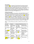 Instrument Blank
(IB)
Internal Standard
(IS) Area Counts
Surrogate Recovery
Beginning and end
of each 12-hour
analytical period
Each sample, blank,
and standard
Each sample, blank,
and standard
Below PCE MDL
or sample values
*5x IB
IS area = 50% -
200% of area that is
•in 1st daily CCS
%R=100±25%
Reanalyze, locate
source of
contamination, flag data
Reanalyze if blank or
standard, flag data
Reanalyze if blank or
standard, flag data
Reconciliation of Data Quality Objectives
A Data Quality Assessment process will be used for reconciliation of DQOs. This process
will consist of the following steps: (1) A review of all data will be conducted to assess the
quality with respect to the QC parameters. Data with QA/QC parameters out of the
acceptance windows will be flagged. Inclusion of qualified data in the data analysis steps
will be based on a thorough review of the data for a particular parameter within the context
of other parameters in that sample and other samples within the same experimental set. (2)
Data that have been verified to be of acceptable quality will be used in a preliminary
review of the results. Basic statistical quantities will be calculated for each of the
experimental sets. This information will be used to identify patterns, relationships, or
potential anomalies. (3) Appropriate statistical procedures for analyzing and summarizing
the data will be identified on the basis of the preliminary review. All assumptions for the
statistical procedures to be used will be identified and verified as acceptable. (4) The
applicable statistical procedures will be performed, interpreted, and any conclusions will be
documented. The data completeness and performance of the experimental design will be
assessed to determine whether or not the data quality and project objectives were met.
References Cited
Denver Instrument Co., 1999, Denver Instrument Company Model 250
pH/Ion/Conductivity Meter Operation Manual, Revision D: Denver Instrument
Company.
Fisher Scientific, 2003, Accumet research model AR60 user manual: Fisher Scientific.
Stanley, T.W. and Verner, S.S., 1985, The U.S. Environmental Protection Agency's Quality
Assurance Program, Philadelphia, PA, American Society for Testing and Materials,
p. 12-19.
Taylor, J.K., 1987, Quality Assurance of Chemical Measurements, Washington, D.C., U.S.
Environmental Protection Agency, p. 1-328.
USEPA, 1971, Method 360.1 (Dissolved Oxygen with Membrane Electrode), Standard
Methods for the Examination of Water and Wastewater.
72
image:
Instrument Blank
(IB)
Internal Standard
(IS) Area Counts
Surrogate Recovery
Beginning and end
of each 12-hour
analytical period
Each sample, blank,
and standard
Each sample, blank,
and standard
Below PCE MDL
or sample values
*5x IB
IS area = 50% -
200% of area that is
•in 1st daily CCS
%R=100±25%
Reanalyze, locate
source of
contamination, flag data
Reanalyze if blank or
standard, flag data
Reanalyze if blank or
standard, flag data
Reconciliation of Data Quality Objectives
A Data Quality Assessment process will be used for reconciliation of DQOs. This process
will consist of the following steps: (1) A review of all data will be conducted to assess the
quality with respect to the QC parameters. Data with QA/QC parameters out of the
acceptance windows will be flagged. Inclusion of qualified data in the data analysis steps
will be based on a thorough review of the data for a particular parameter within the context
of other parameters in that sample and other samples within the same experimental set. (2)
Data that have been verified to be of acceptable quality will be used in a preliminary
review of the results. Basic statistical quantities will be calculated for each of the
experimental sets. This information will be used to identify patterns, relationships, or
potential anomalies. (3) Appropriate statistical procedures for analyzing and summarizing
the data will be identified on the basis of the preliminary review. All assumptions for the
statistical procedures to be used will be identified and verified as acceptable. (4) The
applicable statistical procedures will be performed, interpreted, and any conclusions will be
documented. The data completeness and performance of the experimental design will be
assessed to determine whether or not the data quality and project objectives were met.
References Cited
Denver Instrument Co., 1999, Denver Instrument Company Model 250
pH/Ion/Conductivity Meter Operation Manual, Revision D: Denver Instrument
Company.
Fisher Scientific, 2003, Accumet research model AR60 user manual: Fisher Scientific.
Stanley, T.W. and Verner, S.S., 1985, The U.S. Environmental Protection Agency's Quality
Assurance Program, Philadelphia, PA, American Society for Testing and Materials,
p. 12-19.
Taylor, J.K., 1987, Quality Assurance of Chemical Measurements, Washington, D.C., U.S.
Environmental Protection Agency, p. 1-328.
USEPA, 1971, Method 360.1 (Dissolved Oxygen with Membrane Electrode), Standard
Methods for the Examination of Water and Wastewater.
72
image:
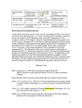 USEPA, 1975, Method 150.1 (pH, Electrometric), 1982 Revision, Standard Methods for
the Examination of Water and Wastewater, 14th Edition.
USEPA, 1996a, Method 8260B, Volatile Organic Compounds by Gas
Chromatography/Mass Spectrometry (GS/MS), Test Methods for Evaluating Solid
Waste, Physical/Chemical Methods (SW-846). 3rd Edition, Final Update I.
USEPA, 1996b, Method 9050A, Specific Conductance, Test Methods for Evaluating Solid
Waste, Physical and Chemical Methods (SW-846), 3rd Edition Final Update.
USEPA, 2004, Method 9040C, pH Electronic Measurement, Test Methods for Evaluating
Solid Waste, Physical/Chemical Methods (SW-846) Final Update IIIB.
Werkema, D.D., 2006, Quality Assurance Project Plan for the Determination of
Geoelectrical Responses to Surfactant Remediation of PCE: Stage 1, Aqueous
Studies, Environmental Sciences Division, NERL-LV, U.S. EPA, p. 1-24.
73
image:
USEPA, 1975, Method 150.1 (pH, Electrometric), 1982 Revision, Standard Methods for
the Examination of Water and Wastewater, 14th Edition.
USEPA, 1996a, Method 8260B, Volatile Organic Compounds by Gas
Chromatography/Mass Spectrometry (GS/MS), Test Methods for Evaluating Solid
Waste, Physical/Chemical Methods (SW-846). 3rd Edition, Final Update I.
USEPA, 1996b, Method 9050A, Specific Conductance, Test Methods for Evaluating Solid
Waste, Physical and Chemical Methods (SW-846), 3rd Edition Final Update.
USEPA, 2004, Method 9040C, pH Electronic Measurement, Test Methods for Evaluating
Solid Waste, Physical/Chemical Methods (SW-846) Final Update IIIB.
Werkema, D.D., 2006, Quality Assurance Project Plan for the Determination of
Geoelectrical Responses to Surfactant Remediation of PCE: Stage 1, Aqueous
Studies, Environmental Sciences Division, NERL-LV, U.S. EPA, p. 1-24.
73
image:
 Appendix B: Standard Operating Procedure pH Meter
U.S Environmental Protection Agency
Office of Research and Development
National Exposure Research Laboratory
Research Triangle Park, North Carolina, Headquarters
Athens, Georgia
Cincinnati, Ohio
Las Vegas, Nevada
STANDARD OPERATING PROCEDURE
Title: pH METER: CALIBRATION AND MEASUREMENTS
Effective Date:01/31/06
Number. CMB12
Author Date: 01/3 1/06
Author
Name: Date Werkema
Title: Physical Scientist, CMB
Signature:'JX, Li
Date:
Approval
Name: Brian Schumacher
Title: CMB Branch Chief
Signature:
Date:
Concurrence1
Name: George Brilis
Title: ESD-LV QA Manager
Signature;,
Date:
/,/.
Optional- typically used by project officers for review by division QA Manager
image:
Appendix B: Standard Operating Procedure pH Meter
U.S Environmental Protection Agency
Office of Research and Development
National Exposure Research Laboratory
Research Triangle Park, North Carolina, Headquarters
Athens, Georgia
Cincinnati, Ohio
Las Vegas, Nevada
STANDARD OPERATING PROCEDURE
Title: pH METER: CALIBRATION AND MEASUREMENTS
Effective Date:01/31/06
Number. CMB12
Author Date: 01/3 1/06
Author
Name: Date Werkema
Title: Physical Scientist, CMB
Signature:'JX, Li
Date:
Approval
Name: Brian Schumacher
Title: CMB Branch Chief
Signature:
Date:
Concurrence1
Name: George Brilis
Title: ESD-LV QA Manager
Signature;,
Date:
/,/.
Optional- typically used by project officers for review by division QA Manager
image:
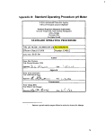 U.S. ENVIRONMENTAL PROTECTION AGENCY
NATIONAL EXPOSURE RESEARCH LABORATORY
CHARACTERIZATION & MONITORING BRANCH
LAS VEGAS, NV
STANDARD OPERATING PROCEDURE CMBXX
ELECTROMETRIC METHOD
for
pH MEASUREMENTS on AQUEOUS MATRICES
Prepared by:.
Dale Werkema, Senior Chemist, CMB
Date
Reviewed by:_
Brian Schumacher, Chief, CMB
Date
Concurrence:
George Brills, QA Officer, ESD - LV
Date
Periodic Review:
75
image:
U.S. ENVIRONMENTAL PROTECTION AGENCY
NATIONAL EXPOSURE RESEARCH LABORATORY
CHARACTERIZATION & MONITORING BRANCH
LAS VEGAS, NV
STANDARD OPERATING PROCEDURE CMBXX
ELECTROMETRIC METHOD
for
pH MEASUREMENTS on AQUEOUS MATRICES
Prepared by:.
Dale Werkema, Senior Chemist, CMB
Date
Reviewed by:_
Brian Schumacher, Chief, CMB
Date
Concurrence:
George Brills, QA Officer, ESD - LV
Date
Periodic Review:
75
image:
 ELECTROMETRIC METHOD for pH MEASUREMENTS
on AQUEOUS MATRICES
1.0 SCOPE and APPLICATION
1.1 This procedure is appropriate for measuring the pH of aqueous samples and
multiphase samples where the aqueous phase is at least 20% of the total sample
volume.
1.2 While the general techniques described in this procedure may be utilized with a
variety of combination pH electrodes, the steps described herein have been
developed for use with an Accumet® glass-body, pH indicating electrode coaxially
joined to a silver/silver chloride reference electrode, in conjunction with a Denver
Instrument Company Model 250 pH/lon/Conductivity Meter.
2.0 SUMMARY of PROCEDURE
The pH of a sample is determined electrometrically using the combination
electrode described above. The meter used to display the results reads the
voltage of the two electrodes and converts it to pH units. The meter is calibrated
using a series of standard solutions, or buffers, of known pH. Temperature
compensation is achieved through the use of an automatic temperature probe
(ATC) in conjunction with the combination electrode.
3.0 HEALTH and SAFETY
3.1 Samples containing organic or inorganic compounds of concern must be disposed
of in an appropriately labeled hazardous waste container. For volatile organic
compounds, rinse the beakers and stirbars with methanol and then with deionized
(Dl) water, discarding both rinsates into the hazardous waste container.
Samples for the geophysics projects containing Dowfax surfactant (extremely toxic
to aquatic life) must also be discarded in the hazardous waste container, followed
by at least two Dl water rinses of the beaker/stirbar into the container.
Wash all beakers and stir bars thoroughly in Micro® detergent followed by 4-5
rinses of hot tap water and 4-5 rinses with Dl water. Allow dishware to air dry.
3.2 Chemicals and chemical handling steps which could be hazardous to laboratory
personnel include the pH 4.00 and 10.0 buffers/standards, and the hydrochloric
acid (HCI) and concentrated ammonium hydroxide (NH4OH) used in cleaning the
glass probe (Section 5). Standard laboratory safety practices, including the use of
gloves, protective eyewear, and closed-toe shoes should be used when handling
samples and laboratory chemicals.
76
image:
ELECTROMETRIC METHOD for pH MEASUREMENTS
on AQUEOUS MATRICES
1.0 SCOPE and APPLICATION
1.1 This procedure is appropriate for measuring the pH of aqueous samples and
multiphase samples where the aqueous phase is at least 20% of the total sample
volume.
1.2 While the general techniques described in this procedure may be utilized with a
variety of combination pH electrodes, the steps described herein have been
developed for use with an Accumet® glass-body, pH indicating electrode coaxially
joined to a silver/silver chloride reference electrode, in conjunction with a Denver
Instrument Company Model 250 pH/lon/Conductivity Meter.
2.0 SUMMARY of PROCEDURE
The pH of a sample is determined electrometrically using the combination
electrode described above. The meter used to display the results reads the
voltage of the two electrodes and converts it to pH units. The meter is calibrated
using a series of standard solutions, or buffers, of known pH. Temperature
compensation is achieved through the use of an automatic temperature probe
(ATC) in conjunction with the combination electrode.
3.0 HEALTH and SAFETY
3.1 Samples containing organic or inorganic compounds of concern must be disposed
of in an appropriately labeled hazardous waste container. For volatile organic
compounds, rinse the beakers and stirbars with methanol and then with deionized
(Dl) water, discarding both rinsates into the hazardous waste container.
Samples for the geophysics projects containing Dowfax surfactant (extremely toxic
to aquatic life) must also be discarded in the hazardous waste container, followed
by at least two Dl water rinses of the beaker/stirbar into the container.
Wash all beakers and stir bars thoroughly in Micro® detergent followed by 4-5
rinses of hot tap water and 4-5 rinses with Dl water. Allow dishware to air dry.
3.2 Chemicals and chemical handling steps which could be hazardous to laboratory
personnel include the pH 4.00 and 10.0 buffers/standards, and the hydrochloric
acid (HCI) and concentrated ammonium hydroxide (NH4OH) used in cleaning the
glass probe (Section 5). Standard laboratory safety practices, including the use of
gloves, protective eyewear, and closed-toe shoes should be used when handling
samples and laboratory chemicals.
76
image:
 4.0 SAMPLE HANDLING and PRESERVATION
4.1 When analyzing 300 mL of aqueous sample for geophysical experiments, place the
liquid matrix and any added experimental components (e.g., PCE, dye) in a 400-
mL beaker with a medium-size stir bar, and cover the beaker tightly with a square
of Parafilm®. Set the beaker on the magnetic stirrer in the laboratory hood and
allow the sample to stir for 5 minutes before introducing the pH and ATC probes.
4.2 If a sample is to be analyzed with other instruments, then cover the sample beaker
tightly with Parafilm® and hold in the hood until the analysis is completed. Dispose
of samples as directed in Section 3.1.
4.3 If subsamples are to collected for GC/MS verification of PCE content, then replace
the Parafilm® on the sample beaker to minimize analyte volatilization after pH
analysis. Collect the sample aliquot with a gas-tight syringe and place it into a
labeled 40-mL glass VOA vial with a screw top and Teflon® septum. At the end of
the day, refrigerate all sample vials at < 4°C until removed for analysis.
5.0 INTERFERENCES and CAUTIONS
5.1 Using the glass electrode probe in strong alkaline solutions will shorten the
electrode life.
5.2 Due to the high resistance of the pH glass membrane, the electrode cable should
not be moved or touched while measurements are being made as unstable
readings may result.
5.3 The level of electrolyte in the inner cavity must be kept above the level of the
solution being measured. The level of the electrolyte should be approximately 1/4
inch below the cap. If the electrolyte level is low add solution from the bottle of
SP135 (4 M KCI saturated with AgCI).
5.4 Temperature effects on pH readings may arise from two sources. The first is the
change in electrode output at various temperatures. This interference can be
controlled by using the ATC probe when taking sample readings. The second is
the change of pH due to changes in the sample as the temperature changes.
Because this error is sample-dependent and cannot be controlled, it is important to
note the temperature along with the pH at the time of analysis.
5.5 As pH electrodes age, a reduction in the Nernstian response may lead to a
sluggish response. This is caused by either contamination of the glass membrane
or by clogging of the liquid junction. The procedures below should improve the
electrode response.
5.5.1 Cleaning the glass pH membrane. A dirty glass membrane is usually
indicated by beads of water forming on the bulb when it is rinsed with Dl
water. The bulb can be cleaned as follows:
• For inorganic deposits-wash with EDTA, ammonia, or acid.
• For grease or similar films-wash with acetone, methanol, or other
appropriate solvent.
77
image:
4.0 SAMPLE HANDLING and PRESERVATION
4.1 When analyzing 300 mL of aqueous sample for geophysical experiments, place the
liquid matrix and any added experimental components (e.g., PCE, dye) in a 400-
mL beaker with a medium-size stir bar, and cover the beaker tightly with a square
of Parafilm®. Set the beaker on the magnetic stirrer in the laboratory hood and
allow the sample to stir for 5 minutes before introducing the pH and ATC probes.
4.2 If a sample is to be analyzed with other instruments, then cover the sample beaker
tightly with Parafilm® and hold in the hood until the analysis is completed. Dispose
of samples as directed in Section 3.1.
4.3 If subsamples are to collected for GC/MS verification of PCE content, then replace
the Parafilm® on the sample beaker to minimize analyte volatilization after pH
analysis. Collect the sample aliquot with a gas-tight syringe and place it into a
labeled 40-mL glass VOA vial with a screw top and Teflon® septum. At the end of
the day, refrigerate all sample vials at < 4°C until removed for analysis.
5.0 INTERFERENCES and CAUTIONS
5.1 Using the glass electrode probe in strong alkaline solutions will shorten the
electrode life.
5.2 Due to the high resistance of the pH glass membrane, the electrode cable should
not be moved or touched while measurements are being made as unstable
readings may result.
5.3 The level of electrolyte in the inner cavity must be kept above the level of the
solution being measured. The level of the electrolyte should be approximately 1/4
inch below the cap. If the electrolyte level is low add solution from the bottle of
SP135 (4 M KCI saturated with AgCI).
5.4 Temperature effects on pH readings may arise from two sources. The first is the
change in electrode output at various temperatures. This interference can be
controlled by using the ATC probe when taking sample readings. The second is
the change of pH due to changes in the sample as the temperature changes.
Because this error is sample-dependent and cannot be controlled, it is important to
note the temperature along with the pH at the time of analysis.
5.5 As pH electrodes age, a reduction in the Nernstian response may lead to a
sluggish response. This is caused by either contamination of the glass membrane
or by clogging of the liquid junction. The procedures below should improve the
electrode response.
5.5.1 Cleaning the glass pH membrane. A dirty glass membrane is usually
indicated by beads of water forming on the bulb when it is rinsed with Dl
water. The bulb can be cleaned as follows:
• For inorganic deposits-wash with EDTA, ammonia, or acid.
• For grease or similar films-wash with acetone, methanol, or other
appropriate solvent.
77
image:
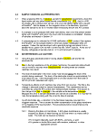 • For proteins-soak in a freshly prepared solution of pepsin in 0.1 N HCI (~
1/4 teaspoon /100 ml) for 30 minutes.
5.5.2 Unblocking the junction. Inspect the reference cavity for crystallization. If
crystallization is present:
• Remove the filling solution by shaking it out through the fill hole.
• Repeatedly rinse the reference cavity with distilled water until all crystals
are dissolved.
• Empty the reference cavity and refill it with SP135.
• Pressurize the electrode (see Accumet® instructions for procedure) and
determine if flow is reestablished.
5.5.3 Unblocking the junction if no crystallization is present or no flow is
reestablished after the above steps:
• Soak the electrode tip in warm water and apply pressure to the filling hole
(see Accumet® instructions for procedure).
• Soak the electrode tip in concentrated ammonium hydroxide for 5-10
minutes (use adequate ventilation). Rinse with deionized
water, and apply pressure to the filling hole. Steps a) and b)
may be repeated as necessary.
• If the junction remains clogged, carefully sand or file the porous plug,
making certain not to contact the glass bulb.
5.5.4 Reconditioning the sensing membrane. This procedure involves the use of
hydrofluoric acid and should not be performed during routine laboratory
operations. The procedure is described in the Accumet electrode
instructions and should only be undertaken by senior chemistry personnel.
6.0 EQUIPMENT and MATERIALS
6.1 pH Meter, Denver Instrument Model 250 pH/lon/Conductivity Meter, or equivalent.
Capable of a minimum of 3-point calibration.
6.2 Combination pH Electrode, Accumet Catalog No. 13-620-285, or equivalent. pH
range of 0 to 14, temperature range of -5 to 110°C.
6.3 pH Buffers, Fisher Scientific standards certified to ± 0.02 pH units, or equivalent.
Minimum of buffers at pH 4.00, pH 7.00, and pH 10.0.
6.4 Automatic Temperature Compensation (ATC) probe, Fisher Catalog No. 13-620-
19, or equivalent. The probe must be accurate to at least ± 0.3° C.
6.5 50-mL glass or disposable plastic beakers.
6.6 400-mL Pyrex® beakers.
6.7 Magnetic stirrer and Teflon® stirbars, various sizes.
6.8 500-mL graduated cylinders for measuring samples.
78
image:
• For proteins-soak in a freshly prepared solution of pepsin in 0.1 N HCI (~
1/4 teaspoon /100 ml) for 30 minutes.
5.5.2 Unblocking the junction. Inspect the reference cavity for crystallization. If
crystallization is present:
• Remove the filling solution by shaking it out through the fill hole.
• Repeatedly rinse the reference cavity with distilled water until all crystals
are dissolved.
• Empty the reference cavity and refill it with SP135.
• Pressurize the electrode (see Accumet® instructions for procedure) and
determine if flow is reestablished.
5.5.3 Unblocking the junction if no crystallization is present or no flow is
reestablished after the above steps:
• Soak the electrode tip in warm water and apply pressure to the filling hole
(see Accumet® instructions for procedure).
• Soak the electrode tip in concentrated ammonium hydroxide for 5-10
minutes (use adequate ventilation). Rinse with deionized
water, and apply pressure to the filling hole. Steps a) and b)
may be repeated as necessary.
• If the junction remains clogged, carefully sand or file the porous plug,
making certain not to contact the glass bulb.
5.5.4 Reconditioning the sensing membrane. This procedure involves the use of
hydrofluoric acid and should not be performed during routine laboratory
operations. The procedure is described in the Accumet electrode
instructions and should only be undertaken by senior chemistry personnel.
6.0 EQUIPMENT and MATERIALS
6.1 pH Meter, Denver Instrument Model 250 pH/lon/Conductivity Meter, or equivalent.
Capable of a minimum of 3-point calibration.
6.2 Combination pH Electrode, Accumet Catalog No. 13-620-285, or equivalent. pH
range of 0 to 14, temperature range of -5 to 110°C.
6.3 pH Buffers, Fisher Scientific standards certified to ± 0.02 pH units, or equivalent.
Minimum of buffers at pH 4.00, pH 7.00, and pH 10.0.
6.4 Automatic Temperature Compensation (ATC) probe, Fisher Catalog No. 13-620-
19, or equivalent. The probe must be accurate to at least ± 0.3° C.
6.5 50-mL glass or disposable plastic beakers.
6.6 400-mL Pyrex® beakers.
6.7 Magnetic stirrer and Teflon® stirbars, various sizes.
6.8 500-mL graduated cylinders for measuring samples.
78
image:
 6.9 SP135 (4 M KCI saturated with AgCI) electrolyte solution.
6.10 Various chemicals for cleaning the electrode: EDTA, ammonia, acetone,
methanol, 0.1 N HCI (~ 1/4 teaspoon /100 ml), concentrated ammonium
hydroxide.
6.11 Deionized water.
7.0 QUALITY CONTROL
7.1 At a minimum, check the measurements of each of the three pH buffers before
beginning sample runs and at the end of the analytical session. If more than 15
samples will be analyzed in one session, then also check the three pH standards
after 8 samples.
For the initial and mid-point readings; if the response of any one of the pH buffers
is greater than ± 0.03 pH units from the nominal value, then an acceptable three-
point calibration must be performed on the meter. If an acceptable calibration
cannot be achieved, then take corrective actions to clean the electrode as
described in Section 5.3. When an acceptable calibration curve has been
established, reanalyze all samples since the last valid standard readings.
If the final buffer checks fail to meet the ± 0.03 units acceptance criterion, then flag
all sample results collected since the last acceptable standard as estimated (J) and
note the circumstances in the lab logbook
7.2 pH values for replicate samples should be within ± 0.05 pH units. If the difference
exceeds that criterion, then flag all pH readings on samples associated with that
sample batch as estimated (J) and note the circumstances in the lab logbook.
7.3 As noted in Section 5.4, the pH electrode is very sensitive to changes in sample
temperature. While the ATC probe provides some compensation for temperature
variation, the temperature reading on the meter must be recorded when the pH is
read on any standards, routine, or QC samples.
8.0 ANALYTICAL PROCEDURES
8.1 Instrument Setup
8.1.1 Verify that the temperature probe (ATC) is plugged into Channel A on the
back of the Denver Instrument Model 250 pH/Conductivity Meter, and the
Accumet glass-body, combination electrode probe is connected to the BNC
connector marked "ch.A." In the menu accessed by the Setup button, the
only parameters of concern are Time (Military), Date, Temperature units
(°C), and Enable strict calibration (OFF).
8.1.2 Press the Standardize button, then select Channel A pH. Verify the
specifications in the Standardize menu, as follows:
Auto-enter Buffer. Do NOT select this option until actual standardization
79
image:
6.9 SP135 (4 M KCI saturated with AgCI) electrolyte solution.
6.10 Various chemicals for cleaning the electrode: EDTA, ammonia, acetone,
methanol, 0.1 N HCI (~ 1/4 teaspoon /100 ml), concentrated ammonium
hydroxide.
6.11 Deionized water.
7.0 QUALITY CONTROL
7.1 At a minimum, check the measurements of each of the three pH buffers before
beginning sample runs and at the end of the analytical session. If more than 15
samples will be analyzed in one session, then also check the three pH standards
after 8 samples.
For the initial and mid-point readings; if the response of any one of the pH buffers
is greater than ± 0.03 pH units from the nominal value, then an acceptable three-
point calibration must be performed on the meter. If an acceptable calibration
cannot be achieved, then take corrective actions to clean the electrode as
described in Section 5.3. When an acceptable calibration curve has been
established, reanalyze all samples since the last valid standard readings.
If the final buffer checks fail to meet the ± 0.03 units acceptance criterion, then flag
all sample results collected since the last acceptable standard as estimated (J) and
note the circumstances in the lab logbook
7.2 pH values for replicate samples should be within ± 0.05 pH units. If the difference
exceeds that criterion, then flag all pH readings on samples associated with that
sample batch as estimated (J) and note the circumstances in the lab logbook.
7.3 As noted in Section 5.4, the pH electrode is very sensitive to changes in sample
temperature. While the ATC probe provides some compensation for temperature
variation, the temperature reading on the meter must be recorded when the pH is
read on any standards, routine, or QC samples.
8.0 ANALYTICAL PROCEDURES
8.1 Instrument Setup
8.1.1 Verify that the temperature probe (ATC) is plugged into Channel A on the
back of the Denver Instrument Model 250 pH/Conductivity Meter, and the
Accumet glass-body, combination electrode probe is connected to the BNC
connector marked "ch.A." In the menu accessed by the Setup button, the
only parameters of concern are Time (Military), Date, Temperature units
(°C), and Enable strict calibration (OFF).
8.1.2 Press the Standardize button, then select Channel A pH. Verify the
specifications in the Standardize menu, as follows:
Auto-enter Buffer. Do NOT select this option until actual standardization
79
image:
 begins.
Manual Buffer Entry. DO NOT USE
Clear Buffers: YES, just prior to calibration; otherwise NO.
Options Menu-
Resolution: 0.01 pH UNITS
Stability Criterion: SLOW (Determines when meter reading is stable
[SI-)
Signal Averaging: VERY SLOW takes the average of 10 readings.
(If the signal is erratic due to changing temperature in the hood,
then this may be set to SLOW.)
Standardization Delay. 60 SECONDS
pH Slope: DEFAULT = 59.16 mV/pH
Manual Temperature Entry. OFF
Data Alarm: OFF
Isopotential Point: DEFAULT = 0.0 mV
Cat Reminder. OFF
Select Buffer Set: CUSTOM BUFFER SET = 4.00, 7.00, 10.0 (May change
slightly as different lots of buffer are used; e.g., 4.01, 9.99.)
8.1.3 Return to the Measurement Screen by pressing the button next to the
"meter" icon, or return to the Standardization Menu by pressing 6)
Standardize menu in the Options Menu.
8.1.4 Add 30 - 40 mL of pH 4.00, 7.00, and 10.0 buffer solutions (certified to ±
0.02 pH units) to labeled 50-mL disposable or glass beakers, and add a
small Teflon® stir bar to each. Use fresh buffer each day; however, the
beakers of buffer used at the beginning of the day may be covered with
Parafilm® to prevent contamination and used for checking the meter
response mid-point in the analyses and at the end of the day.
8.2 Calibration
Remove the pH probe from the storage bottle (pH 7.0 buffer) by loosening the
screw cap slightly and pulling the probe upward. Open the fill hole on the electrode
by turning the ribbed portion at the top of the probe clockwise. Place the pH probe
and the ATC probe in the appropriate holes in the electrode arm, rinse both
thoroughly with Dl water into the waste beaker, and blot (do not rub) off excess
rinsate. Always use care when handling the probe since even a slight scratch on
the glass bulb can leave the electrode useless.
8.2.1 Submerge the probes in the pH 4.00 buffer. The pH electrode probe must
be immersed far enough to cover both the glass sensing bulb and the liquid
junction (the white ceramic dot on the side of the probe). Stir moderately,
and allow the electrode to reach equilibrium, approximately 5 minutes).
After stabilization (an [S] shows by the reading), record the pH and
temperature in the laboratory log book and applicable project report forms.
8.2.2 Push the Standardize button, then select Channel A pH. Select Auto-
enter a buffer, and follow the prompts on the display (already done).
Press Enter.
80
image:
begins.
Manual Buffer Entry. DO NOT USE
Clear Buffers: YES, just prior to calibration; otherwise NO.
Options Menu-
Resolution: 0.01 pH UNITS
Stability Criterion: SLOW (Determines when meter reading is stable
[SI-)
Signal Averaging: VERY SLOW takes the average of 10 readings.
(If the signal is erratic due to changing temperature in the hood,
then this may be set to SLOW.)
Standardization Delay. 60 SECONDS
pH Slope: DEFAULT = 59.16 mV/pH
Manual Temperature Entry. OFF
Data Alarm: OFF
Isopotential Point: DEFAULT = 0.0 mV
Cat Reminder. OFF
Select Buffer Set: CUSTOM BUFFER SET = 4.00, 7.00, 10.0 (May change
slightly as different lots of buffer are used; e.g., 4.01, 9.99.)
8.1.3 Return to the Measurement Screen by pressing the button next to the
"meter" icon, or return to the Standardization Menu by pressing 6)
Standardize menu in the Options Menu.
8.1.4 Add 30 - 40 mL of pH 4.00, 7.00, and 10.0 buffer solutions (certified to ±
0.02 pH units) to labeled 50-mL disposable or glass beakers, and add a
small Teflon® stir bar to each. Use fresh buffer each day; however, the
beakers of buffer used at the beginning of the day may be covered with
Parafilm® to prevent contamination and used for checking the meter
response mid-point in the analyses and at the end of the day.
8.2 Calibration
Remove the pH probe from the storage bottle (pH 7.0 buffer) by loosening the
screw cap slightly and pulling the probe upward. Open the fill hole on the electrode
by turning the ribbed portion at the top of the probe clockwise. Place the pH probe
and the ATC probe in the appropriate holes in the electrode arm, rinse both
thoroughly with Dl water into the waste beaker, and blot (do not rub) off excess
rinsate. Always use care when handling the probe since even a slight scratch on
the glass bulb can leave the electrode useless.
8.2.1 Submerge the probes in the pH 4.00 buffer. The pH electrode probe must
be immersed far enough to cover both the glass sensing bulb and the liquid
junction (the white ceramic dot on the side of the probe). Stir moderately,
and allow the electrode to reach equilibrium, approximately 5 minutes).
After stabilization (an [S] shows by the reading), record the pH and
temperature in the laboratory log book and applicable project report forms.
8.2.2 Push the Standardize button, then select Channel A pH. Select Auto-
enter a buffer, and follow the prompts on the display (already done).
Press Enter.
80
image:
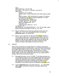 The meter will take readings for 60 seconds, then change to the
Measurement screen and show the reading as 4.00. Again press Enter. If
the signal is unstable (e.g., shows 3.98, 4.01, 4.02) then press Enter when
the reading stabilizes to your acceptable accuracy.
8.2.3 The meter will save the reading and return to the Measurement screen.
Note in the log that the initial reading was changed to 4.00 and the
temperature. Remove the probes from the buffer, rinse thoroughly with Dl
water into the waste beaker, and blot off excess rinsate.
8.2.4 Submerge the probes in the pH 7.00 buffer, stir moderately, and allow the
electrode to reach equilibrium. After stabilization, record the pH and
temperature in the laboratory log book and applicable project report forms.
8.2.5 Push the Standardize button and select Channel A pH. Select Auto-
enter a buffer, and follow the prompts on the display. Press Enter.
The meter will take readings for 60 seconds, then change to the
Measurement screen and show the reading as 7.00. Press Enter and
record the pH and temperature. Remove, rinse, and blot the probes.
8.2.6 Repeat Steps 9.2.4 and 9.2.5 with the pH 10.0 buffer. Then press the Cal
Data button and Channel A....pH. Record the slope of the readings
between the 4.00 and 7.00 buffers, and between the 7.00 and 10.0 buffer.
The slope of each interval must be ^95% to be acceptable. If the slope of
either reading does not meet the calibration criterion, then recalibrate the
meter with fresh standards, or take corrective actions as described below.
Submerge the probes in Dl water while the samples are being prepared for
analysis. If there will be a delay prior to reading the samples, then close
the fill hole on the pH probe and reinsert the probe into the screw-top
storage bottle filled with pH 7.00 buffer. Place the ATC probe in Dl water.
8.3 Sample Measurement
After the standards have been analyzed with acceptable results, routine samples
may be run.
8.3.1 Remove the pH electrode from the storage jar or the Dl water beaker.
Rinse the electrode and ATC probe with Dl water into the waste beaker and
blot lightly. Submerge probes in the sample, begin stirring moderately, and
allow the probes to equilibrate for 5 minutes before taking the reading (use
the clock on the display for timing).
8.3.2 When the response has stabilized ([S] shows next to the reading), record
the pH and the temperature in the laboratory log book and the applicable
project data forms. Rinse the probes thoroughly with Dl water into the
waste beaker, and blot lightly between sample measurements.
81
image:
The meter will take readings for 60 seconds, then change to the
Measurement screen and show the reading as 4.00. Again press Enter. If
the signal is unstable (e.g., shows 3.98, 4.01, 4.02) then press Enter when
the reading stabilizes to your acceptable accuracy.
8.2.3 The meter will save the reading and return to the Measurement screen.
Note in the log that the initial reading was changed to 4.00 and the
temperature. Remove the probes from the buffer, rinse thoroughly with Dl
water into the waste beaker, and blot off excess rinsate.
8.2.4 Submerge the probes in the pH 7.00 buffer, stir moderately, and allow the
electrode to reach equilibrium. After stabilization, record the pH and
temperature in the laboratory log book and applicable project report forms.
8.2.5 Push the Standardize button and select Channel A pH. Select Auto-
enter a buffer, and follow the prompts on the display. Press Enter.
The meter will take readings for 60 seconds, then change to the
Measurement screen and show the reading as 7.00. Press Enter and
record the pH and temperature. Remove, rinse, and blot the probes.
8.2.6 Repeat Steps 9.2.4 and 9.2.5 with the pH 10.0 buffer. Then press the Cal
Data button and Channel A....pH. Record the slope of the readings
between the 4.00 and 7.00 buffers, and between the 7.00 and 10.0 buffer.
The slope of each interval must be ^95% to be acceptable. If the slope of
either reading does not meet the calibration criterion, then recalibrate the
meter with fresh standards, or take corrective actions as described below.
Submerge the probes in Dl water while the samples are being prepared for
analysis. If there will be a delay prior to reading the samples, then close
the fill hole on the pH probe and reinsert the probe into the screw-top
storage bottle filled with pH 7.00 buffer. Place the ATC probe in Dl water.
8.3 Sample Measurement
After the standards have been analyzed with acceptable results, routine samples
may be run.
8.3.1 Remove the pH electrode from the storage jar or the Dl water beaker.
Rinse the electrode and ATC probe with Dl water into the waste beaker and
blot lightly. Submerge probes in the sample, begin stirring moderately, and
allow the probes to equilibrate for 5 minutes before taking the reading (use
the clock on the display for timing).
8.3.2 When the response has stabilized ([S] shows next to the reading), record
the pH and the temperature in the laboratory log book and the applicable
project data forms. Rinse the probes thoroughly with Dl water into the
waste beaker, and blot lightly between sample measurements.
81
image:
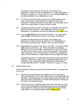 9.0 DOCUMENTATION
9.1 Logbooks and data forms should be used to document laboratory activities. It is
each analyst's responsibility to ensure the accuracy of the entries in any
documents associated with the project, and to complete the logbooks and data
forms as described in the applicable Quality Assurance Project Plan(s).
9.2 For some projects, data will be entered into spreadsheets at a computer terminal in
the laboratory. All of the data transferred to electronic spreadsheets must be
reviewed for accuracy after entry (preferably by a second party) and prior to
statistical analysis and presentation.
10.0 REFERENCES
10.1 EPA. 2004. Method 9040C, pH Electronic Measurement, Revision 3. Test
Methods for Evaluating Solid Waste, Update III. (SW-846). Office of Solid Waste,
U.S. Environmental Protection Agency, Washington, D.C.
10.2 EPA. 1982 Revision. Method 150.1 (pH, Electrometric). Standard Methods for
the Examination of Water and Wastewater, 14th Edition, p 460, 1975.
10.3 Denver Instrument Company. 1999. Operation Manual for Model 250
pH/lon/Conductivity Meter, Revision D. Denver Instrument Company 6542 Fig
Street, Arvada, CO 80004.
82
image:
9.0 DOCUMENTATION
9.1 Logbooks and data forms should be used to document laboratory activities. It is
each analyst's responsibility to ensure the accuracy of the entries in any
documents associated with the project, and to complete the logbooks and data
forms as described in the applicable Quality Assurance Project Plan(s).
9.2 For some projects, data will be entered into spreadsheets at a computer terminal in
the laboratory. All of the data transferred to electronic spreadsheets must be
reviewed for accuracy after entry (preferably by a second party) and prior to
statistical analysis and presentation.
10.0 REFERENCES
10.1 EPA. 2004. Method 9040C, pH Electronic Measurement, Revision 3. Test
Methods for Evaluating Solid Waste, Update III. (SW-846). Office of Solid Waste,
U.S. Environmental Protection Agency, Washington, D.C.
10.2 EPA. 1982 Revision. Method 150.1 (pH, Electrometric). Standard Methods for
the Examination of Water and Wastewater, 14th Edition, p 460, 1975.
10.3 Denver Instrument Company. 1999. Operation Manual for Model 250
pH/lon/Conductivity Meter, Revision D. Denver Instrument Company 6542 Fig
Street, Arvada, CO 80004.
82
image:
 Appendix C: Standard Operating Procedure Conductivity
Meter
U.S Environmental Protection Agency
Office of Research and Development
National Exposure Research Laboratory
Research Triangle Park, North Carolina, Headquarters
Athens, Georgia
Cincinnati, Ohio
Las Vegas, Nevada
STANDARD OPERATING PROCEDURE
Title: CONDUCTIVITY METER: CALIBRATION AND MEASUREMENTS
Effective Date:02/01/06
Number: CMB13
Author Date: 02/01/06
Author
Name: Dale Werkema
Title: Physical Scientist
Signature:
u
Date:
~ / - C (y
Approval
Name: Brian Schumacher
Title: Branch Chief
Signature:
Date:
Concurrence1
Name: George Brilis
Title: ESD-LV QA Manager
Signature:
Date: £--
Optional- typically used by project officers for review by division QA Manager
83
image:
Appendix C: Standard Operating Procedure Conductivity
Meter
U.S Environmental Protection Agency
Office of Research and Development
National Exposure Research Laboratory
Research Triangle Park, North Carolina, Headquarters
Athens, Georgia
Cincinnati, Ohio
Las Vegas, Nevada
STANDARD OPERATING PROCEDURE
Title: CONDUCTIVITY METER: CALIBRATION AND MEASUREMENTS
Effective Date:02/01/06
Number: CMB13
Author Date: 02/01/06
Author
Name: Dale Werkema
Title: Physical Scientist
Signature:
u
Date:
~ / - C (y
Approval
Name: Brian Schumacher
Title: Branch Chief
Signature:
Date:
Concurrence1
Name: George Brilis
Title: ESD-LV QA Manager
Signature:
Date: £--
Optional- typically used by project officers for review by division QA Manager
83
image:
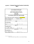 U.S. ENVIRONMENTAL PROTECTION AGENCY
NATIONAL EXPOSURE RESEARCH LABORATORY
CHARACTERIZATION & MONITORING BRANCH
LAS VEGAS, NV
STANDARD OPERATING PROCEDURE CMB13
CONDUCTIVITY MEASUREMENTS
on
AQUEOUS MATRICES
Prepared by:_
Dale Werkema, Physical Scientist, CMB Date Date
Reviewed by:
Brian Schumacher, Chief, CMB Date
Approved by:
George Brills, QA Officer, ESD - LV Date
Periodic Review:
Signature: Title Date
84
image:
U.S. ENVIRONMENTAL PROTECTION AGENCY
NATIONAL EXPOSURE RESEARCH LABORATORY
CHARACTERIZATION & MONITORING BRANCH
LAS VEGAS, NV
STANDARD OPERATING PROCEDURE CMB13
CONDUCTIVITY MEASUREMENTS
on
AQUEOUS MATRICES
Prepared by:_
Dale Werkema, Physical Scientist, CMB Date Date
Reviewed by:
Brian Schumacher, Chief, CMB Date
Approved by:
George Brills, QA Officer, ESD - LV Date
Periodic Review:
Signature: Title Date
84
image:
 CONDUCTIVITY MEASUREMENTS on AQUEOUS MATRICES
1.0 SCOPE and APPLICATION
1.1 This procedure is used to measure conductivity, or the ability of a substance to
conduct electric current. It is applicable to the analysis of aqueous samples and
multiphase samples where the aqueous phase is at least 40% of the total sample
volume.
1.2 While the general techniques described in this procedure may be utilized with a
variety of conductivity probes, the steps described here have been established for
use with a Accumet® plastic-body, 4-cell conductivity electrode. The electrode
probe has a cell constant of 1.0 cm"1, an optimal range of 10 to 2000 /uS/cm, and
integrated automatic temperature compensation (ATC). The conductivity probe is
used in conjunction with a Denver Instrument Company Model 250
pH/lon/Conductivity Meter.
2.0 SUMMARY of PROCEDURE
The conductivity of a sample determined using the 4-cell or 4-band electrode is
based on the measurement of current flowing across the equidistant sensing
elements (bands) in the electrode. When the AC voltage applied across the two
outermost (correcting) bands is equal to the voltage measured in the sample liquid
by the two inner (sensing) bands, the reading produced on the conductivity meter
is corrected for fouling or polarization (which can occur in samples that are high in
conductivity). The meter is calibrated using three or more NIST-traceable standard
solutions of known conductivity.
3.0 HEALTH and SAFETY
3.1 Samples containing organic or inorganic compounds of concern must be disposed
of in an appropriately labeled hazardous waste container. For volatile organic
compounds, rinse the beakers and stirbars with methanol and then with Dl water,
discarding both rinsates into the hazardous waste container.
Samples for the geophysics projects containing Dowfax surfactant (extremely toxic
to aquatic life) must also be discarded in the hazardous waste container, followed
by at least two Dl water rinses of the beaker/stirbar into the container.
Wash all beakers and stir bars thoroughly in Micro® detergent followed by 4-5
rinses of hot tap water and 4-5 rinses with Dl water. Allow dishware to air dry.
3.2 Chemical handling steps which could be hazardous to laboratory personnel include
cleaning the conductivity electrode/probe with various agents. These include: 1%
nitric acid (HNO3), dilute sulfuric (H2SO4) acid, dilute chromic (CrO3) acid, dilute
hydrochloric (HCI) acid, concentrated HCI mixed into 50% isopropanol, acetone,
and a 10% chlorine bleach solution(see Section 5). Standard laboratory safety
85
image:
CONDUCTIVITY MEASUREMENTS on AQUEOUS MATRICES
1.0 SCOPE and APPLICATION
1.1 This procedure is used to measure conductivity, or the ability of a substance to
conduct electric current. It is applicable to the analysis of aqueous samples and
multiphase samples where the aqueous phase is at least 40% of the total sample
volume.
1.2 While the general techniques described in this procedure may be utilized with a
variety of conductivity probes, the steps described here have been established for
use with a Accumet® plastic-body, 4-cell conductivity electrode. The electrode
probe has a cell constant of 1.0 cm"1, an optimal range of 10 to 2000 /uS/cm, and
integrated automatic temperature compensation (ATC). The conductivity probe is
used in conjunction with a Denver Instrument Company Model 250
pH/lon/Conductivity Meter.
2.0 SUMMARY of PROCEDURE
The conductivity of a sample determined using the 4-cell or 4-band electrode is
based on the measurement of current flowing across the equidistant sensing
elements (bands) in the electrode. When the AC voltage applied across the two
outermost (correcting) bands is equal to the voltage measured in the sample liquid
by the two inner (sensing) bands, the reading produced on the conductivity meter
is corrected for fouling or polarization (which can occur in samples that are high in
conductivity). The meter is calibrated using three or more NIST-traceable standard
solutions of known conductivity.
3.0 HEALTH and SAFETY
3.1 Samples containing organic or inorganic compounds of concern must be disposed
of in an appropriately labeled hazardous waste container. For volatile organic
compounds, rinse the beakers and stirbars with methanol and then with Dl water,
discarding both rinsates into the hazardous waste container.
Samples for the geophysics projects containing Dowfax surfactant (extremely toxic
to aquatic life) must also be discarded in the hazardous waste container, followed
by at least two Dl water rinses of the beaker/stirbar into the container.
Wash all beakers and stir bars thoroughly in Micro® detergent followed by 4-5
rinses of hot tap water and 4-5 rinses with Dl water. Allow dishware to air dry.
3.2 Chemical handling steps which could be hazardous to laboratory personnel include
cleaning the conductivity electrode/probe with various agents. These include: 1%
nitric acid (HNO3), dilute sulfuric (H2SO4) acid, dilute chromic (CrO3) acid, dilute
hydrochloric (HCI) acid, concentrated HCI mixed into 50% isopropanol, acetone,
and a 10% chlorine bleach solution(see Section 5). Standard laboratory safety
85
image:
 practices, including the use of gloves, protective eyewear, and closed-toe shoes
should be used when handling samples and laboratory chemicals.
4.0 SAMPLE HANDLING and PRESERVATION
4.1 When analyzing 300 ml of aqueous sample for geophysical experiments, place the
liquid matrix and any added experimental components (e.g., PCE, dye) in a 400-
ml_ beaker with a medium-size stir bar, and cover the beaker tightly with a square
of Parafilm®. Set the beaker on the magnetic stirrer in the laboratory hood and
allow the sample to stir for 5 minutes before introducing the conductivity probe.
4.2 If a sample is to be analyzed with other instruments, then cover the sample beaker
tightly with Parafilm® and hold in the hood until the analysis is completed. When
finished, dispose of samples as directed in Section 3.1.
4.3 If subsamples are to collected for GC/MS verification of PCE content, then replace
the Parafilm® on the sample beaker to minimize analyte volatilization after
conductivity analysis. Collect the sample aliquot with a gas-tight syringe and place
it into a labeled 40-mL glass VGA vial with a screw top and Teflon septum. At the
end of the day, refrigerate all sample vials at < 4°C until removed for GC/MS
analysis.
5.0 INTERFERENCES and CAUTIONS
5.1 Do NOT use the 4-cell probe with the plastic cover with samples containing organic
solvents (e.g., tetrachloroethene or PCE) at concentrations greater than 400 ppm.
5.2 Grease, oil, fingerprints, and other contaminates on the sensing elements may
cause erroneous measurements or sporadic responses. For most applications, a
hot solution of water with a mild lab detergent can be used for cleaning. If this
approach is insufficient, then use the cleaning procedures described below.
5.2.1 1% dilute nitric acid (HNO3) may be used. Dip the electrode in dilute (1%)
nitric acid (HNO3) and agitate for 2 - 3 minutes. Other dilute acids (e.g.,
sulfuric, chromic, hydrochloric) may be used for cleaning; however, NEVER
use aqua regia. Rinse the electrode thoroughly with Dl water after using
the acid.
5.2.2 For a stronger cleaning solution, prepare a solution of concentrated HCI
mixed into 50% isopropanol. Dip the electrode in the solution and agitate.
Rinse the electrode thoroughly with Dl water.
5.2.3 After analyzing samples containing organic fouling agents (e.g., fats, oils)
clean the electrode with acetone. For algae and bacteria-containing
samples, clean the electrode with a 10% chlorine bleach solution.
5.3 Inspect the electrode after each cleaning. If the black coating (platinum black)
appears to be wearing or flaking off the electrode or if the cell constant has
changed by more than 50%, then the cell should be replatinized. This procedure
has the potential to damage the conductivity electrode and should be performed by
86
image:
practices, including the use of gloves, protective eyewear, and closed-toe shoes
should be used when handling samples and laboratory chemicals.
4.0 SAMPLE HANDLING and PRESERVATION
4.1 When analyzing 300 ml of aqueous sample for geophysical experiments, place the
liquid matrix and any added experimental components (e.g., PCE, dye) in a 400-
ml_ beaker with a medium-size stir bar, and cover the beaker tightly with a square
of Parafilm®. Set the beaker on the magnetic stirrer in the laboratory hood and
allow the sample to stir for 5 minutes before introducing the conductivity probe.
4.2 If a sample is to be analyzed with other instruments, then cover the sample beaker
tightly with Parafilm® and hold in the hood until the analysis is completed. When
finished, dispose of samples as directed in Section 3.1.
4.3 If subsamples are to collected for GC/MS verification of PCE content, then replace
the Parafilm® on the sample beaker to minimize analyte volatilization after
conductivity analysis. Collect the sample aliquot with a gas-tight syringe and place
it into a labeled 40-mL glass VGA vial with a screw top and Teflon septum. At the
end of the day, refrigerate all sample vials at < 4°C until removed for GC/MS
analysis.
5.0 INTERFERENCES and CAUTIONS
5.1 Do NOT use the 4-cell probe with the plastic cover with samples containing organic
solvents (e.g., tetrachloroethene or PCE) at concentrations greater than 400 ppm.
5.2 Grease, oil, fingerprints, and other contaminates on the sensing elements may
cause erroneous measurements or sporadic responses. For most applications, a
hot solution of water with a mild lab detergent can be used for cleaning. If this
approach is insufficient, then use the cleaning procedures described below.
5.2.1 1% dilute nitric acid (HNO3) may be used. Dip the electrode in dilute (1%)
nitric acid (HNO3) and agitate for 2 - 3 minutes. Other dilute acids (e.g.,
sulfuric, chromic, hydrochloric) may be used for cleaning; however, NEVER
use aqua regia. Rinse the electrode thoroughly with Dl water after using
the acid.
5.2.2 For a stronger cleaning solution, prepare a solution of concentrated HCI
mixed into 50% isopropanol. Dip the electrode in the solution and agitate.
Rinse the electrode thoroughly with Dl water.
5.2.3 After analyzing samples containing organic fouling agents (e.g., fats, oils)
clean the electrode with acetone. For algae and bacteria-containing
samples, clean the electrode with a 10% chlorine bleach solution.
5.3 Inspect the electrode after each cleaning. If the black coating (platinum black)
appears to be wearing or flaking off the electrode or if the cell constant has
changed by more than 50%, then the cell should be replatinized. This procedure
has the potential to damage the conductivity electrode and should be performed by
86
image:
 senior lab personnel in accordance with the steps outlined in the Accumet
Conductivity Cell Instruction Manual.
5.4 Temperature variation has a substantial effect on conductivity measurements. The
impact diminishes as the ionic strength of the sample solution increases. Even
with the temperature compensation provided by the ATC, there is a delay in the
response of the themistor relative to the almost instantaneous change in the
conductivity that occurs when a liquid has a rapid variation in temperature.
6.0 EQUIPMENT and MATERIALS
6.1 Conductivity Meter, Denver Instrument Model 250 pH/lon/Conductivity Meter, or
equivalent. Capable of a minimum of 3-point calibration.
6.2 Conductivity electrode/probe, Denver Instrument Catalog No. 301047.0, or
equivalent. Plastic body, 4-cell, optimal measurement range of 10 to 5000 //S/cm,
Temperature range of 0 to 80°C.
6.3 Conductivity standards, Fisherbrand® Traceable® calibration standards, or
equivalent. Accurate to ± 0.25% or ± 0.25 /^S. Minimum standards at 10 //S/cm,
100 /^S/cm, and 1000 ^S/cm.
6.4 40-mL glass VOA vials, with Teflon® septa in screw caps.
6.5 400-mL Pyrex® beakers.
6.6 Magnetic stirrer and Teflon® stirbars, various sizes.
6.7 500-mL graduated cylinders for measuring samples
6.8 Various chemicals for cleaning the probe/electrode: 1% nitric acid (HNO3), dilute
sulfuric (H2SO4) acid, dilute chromic (CrO3) acid, dilute hydrochloric (HCI) acid,
concentrated HCI mixed into 50% isopropanol, acetone, 10% chlorine bleach
solution
6.9 Deionized water.
7.0 QUALITY CONTROL
7.1 The measurements of each of the three conductivity standards must be taken
before beginning sample runs. If the standard readings are not within ± 10% of the
respective standard at the beginning of the previous day, then the instrument must
be calibrated and meet the acceptance criteria described in Section 8.2
7.2 At a minimum, recheck the measurements of all three standards at the end of the
analytical session. If more than 15 samples will be analyzed in one session, then
also check the three standards after 8 samples.
For the mid-point and final standard measurements; if the response of any one of
the conductivity standards is greater than ± 10% from the nominal value, then a
87
image:
senior lab personnel in accordance with the steps outlined in the Accumet
Conductivity Cell Instruction Manual.
5.4 Temperature variation has a substantial effect on conductivity measurements. The
impact diminishes as the ionic strength of the sample solution increases. Even
with the temperature compensation provided by the ATC, there is a delay in the
response of the themistor relative to the almost instantaneous change in the
conductivity that occurs when a liquid has a rapid variation in temperature.
6.0 EQUIPMENT and MATERIALS
6.1 Conductivity Meter, Denver Instrument Model 250 pH/lon/Conductivity Meter, or
equivalent. Capable of a minimum of 3-point calibration.
6.2 Conductivity electrode/probe, Denver Instrument Catalog No. 301047.0, or
equivalent. Plastic body, 4-cell, optimal measurement range of 10 to 5000 //S/cm,
Temperature range of 0 to 80°C.
6.3 Conductivity standards, Fisherbrand® Traceable® calibration standards, or
equivalent. Accurate to ± 0.25% or ± 0.25 /^S. Minimum standards at 10 //S/cm,
100 /^S/cm, and 1000 ^S/cm.
6.4 40-mL glass VOA vials, with Teflon® septa in screw caps.
6.5 400-mL Pyrex® beakers.
6.6 Magnetic stirrer and Teflon® stirbars, various sizes.
6.7 500-mL graduated cylinders for measuring samples
6.8 Various chemicals for cleaning the probe/electrode: 1% nitric acid (HNO3), dilute
sulfuric (H2SO4) acid, dilute chromic (CrO3) acid, dilute hydrochloric (HCI) acid,
concentrated HCI mixed into 50% isopropanol, acetone, 10% chlorine bleach
solution
6.9 Deionized water.
7.0 QUALITY CONTROL
7.1 The measurements of each of the three conductivity standards must be taken
before beginning sample runs. If the standard readings are not within ± 10% of the
respective standard at the beginning of the previous day, then the instrument must
be calibrated and meet the acceptance criteria described in Section 8.2
7.2 At a minimum, recheck the measurements of all three standards at the end of the
analytical session. If more than 15 samples will be analyzed in one session, then
also check the three standards after 8 samples.
For the mid-point and final standard measurements; if the response of any one of
the conductivity standards is greater than ± 10% from the nominal value, then a
87
image:
 new three-point calibration must be performed on the meter. If an acceptable
calibration cannot be achieved, then take corrective actions to clean the electrode
as described in Section 5.3. When an acceptable calibration curve has been
established, reanalyze all samples since the last valid standard readings.
7.3 Conductivity values for replicate samples should be within ± 25%. If the difference
exceeds that criterion, then flag all conductivity readings on samples associated
with that sample batch as estimated (J) and note the circumstances in the lab
logbook.
7.4 As noted in Section 5.4, the conductivity electrode/probe is very sensitive to
changes in sample temperature. While the ATC provides compensation for
temperature variation, the temperature reading on the meter must be recorded
when the conductivity is read on any standards, routine, or QC samples.
8.0 ANALYTICAL PROCEDURES
8.1 Instrument Setup
8.1.1 Verify that the Denver Instrument 4-cell conductivity probe is connected to
the Channel C/ Conductivity DIN on the back of the Denver Instrument
Model 250 pH/Conductivity Meter. In the menu accessed by the Setup
button, the parameters of concern are Time (Military), Date, Temperature
units (°C), and Enable strict calibration (OFF).
8.1.2 Press the Standardize button, then select Channel C Conductivity. In
the Standardize Menu select 4) Options. Verify the specifications in the
Options Menu, as follows:
Resolution: 3 significant digits
Stability Criterion: SLOW (Determines when the meter reading is stable
[S].)
Signal Averaging: SLOW (Takes average of 8 readings.)
Standardization Delay. 60 seconds
Cell Constant: 1.0 cm"1 for the 4-cell probe
Manual Temperature Entry. OFF
Data Alarm: OFF
Display Units: /uS/cm
Reference Temperature: 25°
Temperature Coefficient: DEFAULT = 1.90 % / °C
8.1.3 Return to the Measurement Screen by pressing the button next to the
"meter" icon, or return to the Standardization Menu by pressing 6)
Standardize menu in the Options Menu.
8.1.4 Label three 40-mL VOA vials with the concentrations of the three calibration
standards (i.e., 10 /^S/cm, 100 ^S/cm, 1000 //S/cm). Fill the vials to the
shoulder with the appropriate standard and add a small stir bar. Cap each
standard tightly and place in the laboratory hood to equilibrate with the
ambient temperature.
image:
new three-point calibration must be performed on the meter. If an acceptable
calibration cannot be achieved, then take corrective actions to clean the electrode
as described in Section 5.3. When an acceptable calibration curve has been
established, reanalyze all samples since the last valid standard readings.
7.3 Conductivity values for replicate samples should be within ± 25%. If the difference
exceeds that criterion, then flag all conductivity readings on samples associated
with that sample batch as estimated (J) and note the circumstances in the lab
logbook.
7.4 As noted in Section 5.4, the conductivity electrode/probe is very sensitive to
changes in sample temperature. While the ATC provides compensation for
temperature variation, the temperature reading on the meter must be recorded
when the conductivity is read on any standards, routine, or QC samples.
8.0 ANALYTICAL PROCEDURES
8.1 Instrument Setup
8.1.1 Verify that the Denver Instrument 4-cell conductivity probe is connected to
the Channel C/ Conductivity DIN on the back of the Denver Instrument
Model 250 pH/Conductivity Meter. In the menu accessed by the Setup
button, the parameters of concern are Time (Military), Date, Temperature
units (°C), and Enable strict calibration (OFF).
8.1.2 Press the Standardize button, then select Channel C Conductivity. In
the Standardize Menu select 4) Options. Verify the specifications in the
Options Menu, as follows:
Resolution: 3 significant digits
Stability Criterion: SLOW (Determines when the meter reading is stable
[S].)
Signal Averaging: SLOW (Takes average of 8 readings.)
Standardization Delay. 60 seconds
Cell Constant: 1.0 cm"1 for the 4-cell probe
Manual Temperature Entry. OFF
Data Alarm: OFF
Display Units: /uS/cm
Reference Temperature: 25°
Temperature Coefficient: DEFAULT = 1.90 % / °C
8.1.3 Return to the Measurement Screen by pressing the button next to the
"meter" icon, or return to the Standardization Menu by pressing 6)
Standardize menu in the Options Menu.
8.1.4 Label three 40-mL VOA vials with the concentrations of the three calibration
standards (i.e., 10 /^S/cm, 100 ^S/cm, 1000 //S/cm). Fill the vials to the
shoulder with the appropriate standard and add a small stir bar. Cap each
standard tightly and place in the laboratory hood to equilibrate with the
ambient temperature.
image:
 8.2 Calibration
(Note: Conductivity standards cannot be diluted; conductivity does not dilute
linearly.)
When running samples intermittently, calibrate the instrument with fresh standards
for each use. When samples are being analyzed daily, the standard solutions MAY
be used for a second day without recalibrating the instrument^ readings at each
level are within ± 10% of the respective readings at the beginning of the previous
day.
8.2.1 Remove the conductivity probe from the storage water beaker and place it
in a hole on the electrode arm. Rinse the probe with Dl water (into the
waste beaker), and blot off excess rinsate. Remove the screw top from the
VOA vial containing the first standard (10 /wS/cm) and stand the vial in a
150-mL beaker on the stir plate.
8.2.2 Submerge the probe in the standard far enough to completely cover the
holes in the sides of the plastic sheath protecting the glass electrode.
Bubbles should be seen coming from one or both holes as the air is
displaced. Then lift the probe completely out of the standard so that the
liquid between the electrode and the plastic cover drains out. Reimmerse
the probe to cover the holes and again lift it from the liquid to drain. Repeat
the immersion one more time. If bubbles are not observed escaping, then
tap the plastic sheath to dislodge the air. Stir moderately, and allow the cell
to reach equilibrium for about 3-5 minutes. After stabilization (make sure
an [S] shows by the reading), record the conductivity and temperature in
the laboratory log book and on applicable project report forms.
8.2.3 Press the Standardize button, then select Channel C Conductivity. In
the Menu press 3) Clear Standards and select YES. Then press 1) Enter
a Standard. Type in the concentration of the standard to be measured
(e.g., 10.0) and press Enter.
The meter will take readings for 60 seconds, then change to the
Measurement Screen and show the reading. Again press Enter. Note: the
standard reading may not be identical to the concentration entered above
due to the probe's temperature compensation feature.
8.2.4 The meter will save the reading and return to the Measurement Screen.
Note the final reading and temperature in the logbook. Remove the probe
from the standard, rinse thoroughly with Dl water into the waste beaker,
and blot off the rinse water. Be sure to tightly cap the standard vial for later
use.
8.2.5 Submerge the probe three times in the second (100 /uS/cm) standard as
described in Steps 8.2.1 and 8.2.2, stir moderately, and again allow the cell
to reach equilibrium for about.3 - 5 minutes. After stabilization, record the
pH and temperature in the log book.
89
image:
8.2 Calibration
(Note: Conductivity standards cannot be diluted; conductivity does not dilute
linearly.)
When running samples intermittently, calibrate the instrument with fresh standards
for each use. When samples are being analyzed daily, the standard solutions MAY
be used for a second day without recalibrating the instrument^ readings at each
level are within ± 10% of the respective readings at the beginning of the previous
day.
8.2.1 Remove the conductivity probe from the storage water beaker and place it
in a hole on the electrode arm. Rinse the probe with Dl water (into the
waste beaker), and blot off excess rinsate. Remove the screw top from the
VOA vial containing the first standard (10 /wS/cm) and stand the vial in a
150-mL beaker on the stir plate.
8.2.2 Submerge the probe in the standard far enough to completely cover the
holes in the sides of the plastic sheath protecting the glass electrode.
Bubbles should be seen coming from one or both holes as the air is
displaced. Then lift the probe completely out of the standard so that the
liquid between the electrode and the plastic cover drains out. Reimmerse
the probe to cover the holes and again lift it from the liquid to drain. Repeat
the immersion one more time. If bubbles are not observed escaping, then
tap the plastic sheath to dislodge the air. Stir moderately, and allow the cell
to reach equilibrium for about 3-5 minutes. After stabilization (make sure
an [S] shows by the reading), record the conductivity and temperature in
the laboratory log book and on applicable project report forms.
8.2.3 Press the Standardize button, then select Channel C Conductivity. In
the Menu press 3) Clear Standards and select YES. Then press 1) Enter
a Standard. Type in the concentration of the standard to be measured
(e.g., 10.0) and press Enter.
The meter will take readings for 60 seconds, then change to the
Measurement Screen and show the reading. Again press Enter. Note: the
standard reading may not be identical to the concentration entered above
due to the probe's temperature compensation feature.
8.2.4 The meter will save the reading and return to the Measurement Screen.
Note the final reading and temperature in the logbook. Remove the probe
from the standard, rinse thoroughly with Dl water into the waste beaker,
and blot off the rinse water. Be sure to tightly cap the standard vial for later
use.
8.2.5 Submerge the probe three times in the second (100 /uS/cm) standard as
described in Steps 8.2.1 and 8.2.2, stir moderately, and again allow the cell
to reach equilibrium for about.3 - 5 minutes. After stabilization, record the
pH and temperature in the log book.
89
image:
 8.2.6 Push the Standardize button, then select Channel C Conductivity. Do
NOT press Clear Standards, but select 1) Enter a Standard. Again, type in
the concentration of the standard to be measured (e.g., 100.0) and press
Enter.
The meter will take readings for 60 seconds, then change to the
Measurement Screen and show the reading. Press Enter and record the
conductivity and temperature. Remove, rinse, and blot the probe.
8.2.7 Repeat Steps 8.2.5 and 8.2.6 with the third (1000 ^S/cm) and any
additional standards (up to five standards may be used for calibration to
cover the expected range of the sample results). Press the Cal Data button
and Channel C....Conductivity to display the cell constants for each
standard. The standards should be a factor of 10 apart in conductivity and
within ± 20% of their nominal value. If the standards exceed these limits,
then corrective actions should be taken.
After calibration, rinse the probe and submerge it in Dl water until samples
are ready for analysis. The water should cover the holes in the plastic
cover at all times.
8.3 Sample Measurement
After the standards have been analyzed with acceptable results, routine samples
may be run.
8.3.1 Submerge the probe in the sample to cover the holes in the plastic cover,
remove from the liquid and allow to drain, and repeat at least two times,
ensuring that all air bubbles have been driven out of the probe sheath.
Allow the probe to equilibrate for 5 minutes before taking the reading (use
the clock on the display for timing).
8.3.2 When the response has stabilized ([S] next to the reading), record the
conductivity and the temperature in the laboratory log book and on any
applicable project data forms. Rinse the probe thoroughly both inside and
outside the plastic sheath with Dl water and blot dry between sample
measurements.
8.3.3 If the probe will not be used for an extended period of time after analyzing
the samples, then disconnect it from the meter and store it dry. Soak the
cell in Dl or distilled water for at least 10 minutes prior to use.
9.0 DOCUMENTATION
9.1 Logbooks and data forms should be used to document laboratory activities. It is
each analyst's responsibility to ensure the accuracy of the entries in any
documents associated with the project, and to complete the logbooks and data
forms as described in the applicable Quality Assurance Project Plan(s).
9.2 For some projects, data will be entered into spreadsheets at a computer terminal in
the laboratory. All data transferred to electronic spreadsheets must be reviewed
90
image:
8.2.6 Push the Standardize button, then select Channel C Conductivity. Do
NOT press Clear Standards, but select 1) Enter a Standard. Again, type in
the concentration of the standard to be measured (e.g., 100.0) and press
Enter.
The meter will take readings for 60 seconds, then change to the
Measurement Screen and show the reading. Press Enter and record the
conductivity and temperature. Remove, rinse, and blot the probe.
8.2.7 Repeat Steps 8.2.5 and 8.2.6 with the third (1000 ^S/cm) and any
additional standards (up to five standards may be used for calibration to
cover the expected range of the sample results). Press the Cal Data button
and Channel C....Conductivity to display the cell constants for each
standard. The standards should be a factor of 10 apart in conductivity and
within ± 20% of their nominal value. If the standards exceed these limits,
then corrective actions should be taken.
After calibration, rinse the probe and submerge it in Dl water until samples
are ready for analysis. The water should cover the holes in the plastic
cover at all times.
8.3 Sample Measurement
After the standards have been analyzed with acceptable results, routine samples
may be run.
8.3.1 Submerge the probe in the sample to cover the holes in the plastic cover,
remove from the liquid and allow to drain, and repeat at least two times,
ensuring that all air bubbles have been driven out of the probe sheath.
Allow the probe to equilibrate for 5 minutes before taking the reading (use
the clock on the display for timing).
8.3.2 When the response has stabilized ([S] next to the reading), record the
conductivity and the temperature in the laboratory log book and on any
applicable project data forms. Rinse the probe thoroughly both inside and
outside the plastic sheath with Dl water and blot dry between sample
measurements.
8.3.3 If the probe will not be used for an extended period of time after analyzing
the samples, then disconnect it from the meter and store it dry. Soak the
cell in Dl or distilled water for at least 10 minutes prior to use.
9.0 DOCUMENTATION
9.1 Logbooks and data forms should be used to document laboratory activities. It is
each analyst's responsibility to ensure the accuracy of the entries in any
documents associated with the project, and to complete the logbooks and data
forms as described in the applicable Quality Assurance Project Plan(s).
9.2 For some projects, data will be entered into spreadsheets at a computer terminal in
the laboratory. All data transferred to electronic spreadsheets must be reviewed
90
image:
 for accuracy after entry (preferably by a second party) and prior to statistical
analysis and presentation.
10.0 REFERENCES
10.1 EPA. 1996. Method 9050A, Specific Conductance. Revision 1. Test Methods for
Evaluation Solid Wastes, Update III (SW-846). Office of Solid Waste, U.S.
Environmental Protection Agency, Washington, D.C.
10.2 EPA. 1985. Method 205, Conductivity. Standard Methods for the Examination of
Water and Wastewater, 16th ed.
10.3 Denver Instrument Company. 1999. Operation Manual for Model 250
pH/lon/Conductivity Meter, Revision D. Denver Instrument Company 6542 Fig
Street, Arvada, CO 80004.
10.4 Denver Instrument Company. 2005. Conductivity Cell Instruction Manual. Denver
Instrument Company 6542 Fig Street, Arvada, CO 80004.
91
image:
for accuracy after entry (preferably by a second party) and prior to statistical
analysis and presentation.
10.0 REFERENCES
10.1 EPA. 1996. Method 9050A, Specific Conductance. Revision 1. Test Methods for
Evaluation Solid Wastes, Update III (SW-846). Office of Solid Waste, U.S.
Environmental Protection Agency, Washington, D.C.
10.2 EPA. 1985. Method 205, Conductivity. Standard Methods for the Examination of
Water and Wastewater, 16th ed.
10.3 Denver Instrument Company. 1999. Operation Manual for Model 250
pH/lon/Conductivity Meter, Revision D. Denver Instrument Company 6542 Fig
Street, Arvada, CO 80004.
10.4 Denver Instrument Company. 2005. Conductivity Cell Instruction Manual. Denver
Instrument Company 6542 Fig Street, Arvada, CO 80004.
91
image:
 Appendix D: Standard Operating Procedure Dissolved
Oxygen Meter
U.S Environmental Protection Agency
Office of Research and Development
National Exposure Research Laboratory
Research Triangle Park, North Carolina, Headquarters
Athens, Georgia
Cincinnati, Ohio
Las Vegas, Nevada
STANDARD OPERATING PROCEDURE
Title: DISSOLVED OXYGEN METER: CALIBRATION AND MEASUREMENTS
Effective Date:02/02/06
Author Date: 02/02/06
Number: CMB14
Author
Name: Dale Werkema
Title: Physical Scientist
Signature:
6 (•<
Name: Brian Schumacher
Title: Branch Chief, CMB
Signature:
Name: George Brilis
Title: ESD-LV QA Manager
Signature:
Date:
Approval
Pate: 2-£ ~
Concurrence1
Date:
Optional- typically used by project officers for review by division QA Manager
92
image:
Appendix D: Standard Operating Procedure Dissolved
Oxygen Meter
U.S Environmental Protection Agency
Office of Research and Development
National Exposure Research Laboratory
Research Triangle Park, North Carolina, Headquarters
Athens, Georgia
Cincinnati, Ohio
Las Vegas, Nevada
STANDARD OPERATING PROCEDURE
Title: DISSOLVED OXYGEN METER: CALIBRATION AND MEASUREMENTS
Effective Date:02/02/06
Author Date: 02/02/06
Number: CMB14
Author
Name: Dale Werkema
Title: Physical Scientist
Signature:
6 (•<
Name: Brian Schumacher
Title: Branch Chief, CMB
Signature:
Name: George Brilis
Title: ESD-LV QA Manager
Signature:
Date:
Approval
Pate: 2-£ ~
Concurrence1
Date:
Optional- typically used by project officers for review by division QA Manager
92
image:
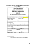 U.S. ENVIRONMENTAL PROTECTION AGENCY
NATIONAL EXPOSURE RESEARCH LABORATORY
CHARACTERIZATION & MONITORING BRANCH
LAS VEGAS, NV
STANDARD OPERATING PROCEDURE CMBXX
DISSOLVED OXYGEN MEASUREMENTS
on
AQUEOUS MATRICES
Prepared by:.
Dale Werkema, Research Physical Scientist, CMS . Date
Reviewed by:
Brian Schumacher, Chief, CMB Date
Concurrence by:_
George Brilis, QA Officer, ESD - LV Date
Periodic Review:
93
image:
U.S. ENVIRONMENTAL PROTECTION AGENCY
NATIONAL EXPOSURE RESEARCH LABORATORY
CHARACTERIZATION & MONITORING BRANCH
LAS VEGAS, NV
STANDARD OPERATING PROCEDURE CMBXX
DISSOLVED OXYGEN MEASUREMENTS
on
AQUEOUS MATRICES
Prepared by:.
Dale Werkema, Research Physical Scientist, CMS . Date
Reviewed by:
Brian Schumacher, Chief, CMB Date
Concurrence by:_
George Brilis, QA Officer, ESD - LV Date
Periodic Review:
93
image:
 DISSOLVED OXYGEN MEASUREMENTS on AQUEOUS MATRICES
1.0 SCOPE and APPLICATION
1.1 This procedure is used to measure the concentration of dissolved oxygen (DO) in
aqueous samples. Analytical results can be expressed in mg/L of oxygen, ppm, or
in percent saturation.
1.2 While the general techniques described in this procedure may be utilized with a
variety of DO sensors or probes, the steps described here have been established
for use with a Fisher Scientific / Accumet® biological oxygen demand (BOD) probe.
The polarographic probe is self-stirring, with an operating temperature range of 15
to 35°C. Used in conjunction with an Accumet AR50 pH/conductivity/DO meter,
the DO probe has integrated automatic temperature compensation (ATC). This
probe is not waterproof and is intended only for laboratory use.
2.0 SUMMARY of PROCEDURE
DO measurement is an electrometric method based on the theory that for a given
partial pressure of oxygen in air, the concentration of DO in saturated pure water is
fixed at any one temperature. The probe contains a gold cathode, silver anode
(reference electrode), and supporting electrolyte separated from the sample by an
oxygen-permeable membrane. Oxygen is reduced within the membrane cap with
the reduction current directly proportional to the partial pressure of oxygen in an
aqueous solution. By measuring the partial pressure of oxygen and correcting for
temperature and salinity, the meter produces a reading of oxygen concentration in
the sample. The oxygen readings from the probe are checked at high (> 94%
saturation) and low (< 3% saturation) concentrations prior to and following sample
analysis.
3.0 HEALTH and SAFETY
3.1 Samples containing organic or inorganic compounds of concern must be disposed
of in an appropriately labeled hazardous waste container. For volatile organic
compounds, rinse the beakers and stirbars with methanol and then with Dl water,
discarding both rinsates into the hazardous waste container.
Samples for the geophysics projects containing Dowfax surfactant (extremely toxic
to aquatic life) must also be discarded in the hazardous waste container, followed
by at least two Dl water rinses of the beaker/stirbar into the container.
Wash all beakers and stir bars thoroughly in Micro® detergent followed by 4-5
rinses of hot tap water and 4-5 rinses with Dl water. Allow dishware to air dry.
3.2 Laboratory personnel should use care when preparing or using 14% ammonium
hydroxide to clean the silver anode of the DO probe. Standard laboratory safety
practices, including the use of gloves, protective eyewear, and closed-toe shoes
94
image:
DISSOLVED OXYGEN MEASUREMENTS on AQUEOUS MATRICES
1.0 SCOPE and APPLICATION
1.1 This procedure is used to measure the concentration of dissolved oxygen (DO) in
aqueous samples. Analytical results can be expressed in mg/L of oxygen, ppm, or
in percent saturation.
1.2 While the general techniques described in this procedure may be utilized with a
variety of DO sensors or probes, the steps described here have been established
for use with a Fisher Scientific / Accumet® biological oxygen demand (BOD) probe.
The polarographic probe is self-stirring, with an operating temperature range of 15
to 35°C. Used in conjunction with an Accumet AR50 pH/conductivity/DO meter,
the DO probe has integrated automatic temperature compensation (ATC). This
probe is not waterproof and is intended only for laboratory use.
2.0 SUMMARY of PROCEDURE
DO measurement is an electrometric method based on the theory that for a given
partial pressure of oxygen in air, the concentration of DO in saturated pure water is
fixed at any one temperature. The probe contains a gold cathode, silver anode
(reference electrode), and supporting electrolyte separated from the sample by an
oxygen-permeable membrane. Oxygen is reduced within the membrane cap with
the reduction current directly proportional to the partial pressure of oxygen in an
aqueous solution. By measuring the partial pressure of oxygen and correcting for
temperature and salinity, the meter produces a reading of oxygen concentration in
the sample. The oxygen readings from the probe are checked at high (> 94%
saturation) and low (< 3% saturation) concentrations prior to and following sample
analysis.
3.0 HEALTH and SAFETY
3.1 Samples containing organic or inorganic compounds of concern must be disposed
of in an appropriately labeled hazardous waste container. For volatile organic
compounds, rinse the beakers and stirbars with methanol and then with Dl water,
discarding both rinsates into the hazardous waste container.
Samples for the geophysics projects containing Dowfax surfactant (extremely toxic
to aquatic life) must also be discarded in the hazardous waste container, followed
by at least two Dl water rinses of the beaker/stirbar into the container.
Wash all beakers and stir bars thoroughly in Micro® detergent followed by 4-5
rinses of hot tap water and 4-5 rinses with Dl water. Allow dishware to air dry.
3.2 Laboratory personnel should use care when preparing or using 14% ammonium
hydroxide to clean the silver anode of the DO probe. Standard laboratory safety
practices, including the use of gloves, protective eyewear, and closed-toe shoes
94
image:
 should be used when handling samples and laboratory chemicals.
4.0 SAMPLE HANDLING and PRESERVATION
4.1 When analyzing 300 ml of aqueous sample for geophysical experiments, place the
liquid matrix and any added experimental components (e.g., PCE, dye) in a 400-
mL beaker with a medium-size stir bar, and cover the beaker tightly with a square
of Parafilm®. Set the beaker on the magnetic stirrer in the laboratory hood and
allow the sample to stir for 5 minutes before introducing the DO probe. Because
Cl~ ions are released when the probe is placed in a solution, measurements of pH
and conductivity should be made prior to the determination of DO.
4.2 If subsamples are to collected for GC/MS verification of PCE content, then replace
the Parafilm® on the sample beaker to minimize analyte volatilization after DO
analysis. Collect the sample aliquot with a gas-tight syringe and place it into a
labeled 40-mL glass VGA vial with a screw top and Teflon® septum. At the end of
the day, refrigerate all of the sample vials at < 4°C until removed for GC/MS
analysis.
4.3 When finished, dispose of the samples as directed in Section 3.1
5.0 INTERFERENCES and CAUTIONS
5.1 Temperature variation has a substantial effect on DO: as the temperature
increases the oxygen saturation of water decreases. Even with the temperature
compensation provided by the ATC, there is a delay in the instrument response.
For the Fisher/Accumet probe, a typical response to ADO at 20°C is 90% of the
change in 30 seconds. The temperature at the time of analysis must be noted with
the sample data.
5.2 The presence of dissolved salts limits the amount of oxygen that can dissolve in
water. If salts are known to be present in the sample, then the salinity should be
determined and entered into the instrument in the "Setup" Menu (See Section
8.1.2) and noted with the sample data. Also, conversion factors for solutions
containing salts may be calculated from dissolved oxygen saturation versus salinity
data.
5.3 Hydrogen sulfide, sulfur dioxide, halogens, carbon monoxide, nitric oxide and
nitrous oxide can cause the probe to give erroneous readings. Also, do not use the
probe in any sample that may contain concentrated acids, caustics, and strong
solvents; these substances may damage the FEP Teflon®, rubber, ABS plastic,
and stainless steel components of the probe.
5.4 Reactive gases which pass through the membrane probes may cause
interferences. Chlorine will depolarize the cathode and cause a high probe-output.
Long-term exposures to chlorine will coat the anode with the chloride of the anode
metal (silver) and eventually desensitize the probe. Alkaline samples in which free
chlorine does not exist will not interfere.
6.0 EQUIPMENT and MATERIALS
95
image:
should be used when handling samples and laboratory chemicals.
4.0 SAMPLE HANDLING and PRESERVATION
4.1 When analyzing 300 ml of aqueous sample for geophysical experiments, place the
liquid matrix and any added experimental components (e.g., PCE, dye) in a 400-
mL beaker with a medium-size stir bar, and cover the beaker tightly with a square
of Parafilm®. Set the beaker on the magnetic stirrer in the laboratory hood and
allow the sample to stir for 5 minutes before introducing the DO probe. Because
Cl~ ions are released when the probe is placed in a solution, measurements of pH
and conductivity should be made prior to the determination of DO.
4.2 If subsamples are to collected for GC/MS verification of PCE content, then replace
the Parafilm® on the sample beaker to minimize analyte volatilization after DO
analysis. Collect the sample aliquot with a gas-tight syringe and place it into a
labeled 40-mL glass VGA vial with a screw top and Teflon® septum. At the end of
the day, refrigerate all of the sample vials at < 4°C until removed for GC/MS
analysis.
4.3 When finished, dispose of the samples as directed in Section 3.1
5.0 INTERFERENCES and CAUTIONS
5.1 Temperature variation has a substantial effect on DO: as the temperature
increases the oxygen saturation of water decreases. Even with the temperature
compensation provided by the ATC, there is a delay in the instrument response.
For the Fisher/Accumet probe, a typical response to ADO at 20°C is 90% of the
change in 30 seconds. The temperature at the time of analysis must be noted with
the sample data.
5.2 The presence of dissolved salts limits the amount of oxygen that can dissolve in
water. If salts are known to be present in the sample, then the salinity should be
determined and entered into the instrument in the "Setup" Menu (See Section
8.1.2) and noted with the sample data. Also, conversion factors for solutions
containing salts may be calculated from dissolved oxygen saturation versus salinity
data.
5.3 Hydrogen sulfide, sulfur dioxide, halogens, carbon monoxide, nitric oxide and
nitrous oxide can cause the probe to give erroneous readings. Also, do not use the
probe in any sample that may contain concentrated acids, caustics, and strong
solvents; these substances may damage the FEP Teflon®, rubber, ABS plastic,
and stainless steel components of the probe.
5.4 Reactive gases which pass through the membrane probes may cause
interferences. Chlorine will depolarize the cathode and cause a high probe-output.
Long-term exposures to chlorine will coat the anode with the chloride of the anode
metal (silver) and eventually desensitize the probe. Alkaline samples in which free
chlorine does not exist will not interfere.
6.0 EQUIPMENT and MATERIALS
95
image:
 6.1 DO Meter, Accumet® Research Model AR 50 pH/mV/lon/Conductivity/DO Meter, or
equivalent.
6.2 BOD Probe with stir paddle, Fisher Scientific Catalog No. 13-620-SSP, or
equivalent. DO accuracy of ± 0.1 mg/L or 2% or reading, whichever is greater,
Temperature range of 15 to 35°C.
6.3 BOD Probe Membrane Kit, Fisher Scientific Catalog No. 13-637-DOM, or
equivalent.
6.4 0.08M Sodium sulfite (Na2SO3), for Zero Check Standard.
6.5 40-mL glass VOA vials, with Teflon® septa in screw caps.
6.6 400-mL Pyrex® beakers.
6.7 Teflon® stirbars, small size.
6.8 500-mL graduated cylinders for measuring samples.
6.9 Ammonium hydroxide, 14% for cleaning the silver anode.
6.10 Deionized water.
7.0 QUALITY CONTROL
7.1 Calibrate with the Water-Saturated Air Standard and verify the response of the
Zero Check Standard before beginning sample runs. Check both standards at the
end of the analytical session. When more than 15 samples are to be analyzed in
one session, also verify both standard responses after 8 samples. If either
standard results falls outside of acceptance limits (>94%, and <3%, respectively) at
the mid-point or the end of the analyses, then recalibrate the DO meter and
reanalyze all of the samples run since the last acceptable standard. If standard
results continue to exceed the acceptance limits, then take corrective actions as
described below.
7.2 When analyzing samples prepared in a single surfactant, the percent difference
(%D) between two sample values should be <;15%. The results of replicate
samples analyses must be <15%. If the difference exceeds 15%, then note the
pertinent results in the laboratory logbook and in the project QA report.
7.3 As noted in Section 5.3, the DO probe is sensitive to changes in sample
temperature. While the ATC provides compensation for temperature variation, the
temperature reading on the meter must be recorded when the DO is read on any
standards, routine, or QC samples.
8.0 ANALYTICAL PROCEDURES
8.1 Instrument Setup
96
image:
6.1 DO Meter, Accumet® Research Model AR 50 pH/mV/lon/Conductivity/DO Meter, or
equivalent.
6.2 BOD Probe with stir paddle, Fisher Scientific Catalog No. 13-620-SSP, or
equivalent. DO accuracy of ± 0.1 mg/L or 2% or reading, whichever is greater,
Temperature range of 15 to 35°C.
6.3 BOD Probe Membrane Kit, Fisher Scientific Catalog No. 13-637-DOM, or
equivalent.
6.4 0.08M Sodium sulfite (Na2SO3), for Zero Check Standard.
6.5 40-mL glass VOA vials, with Teflon® septa in screw caps.
6.6 400-mL Pyrex® beakers.
6.7 Teflon® stirbars, small size.
6.8 500-mL graduated cylinders for measuring samples.
6.9 Ammonium hydroxide, 14% for cleaning the silver anode.
6.10 Deionized water.
7.0 QUALITY CONTROL
7.1 Calibrate with the Water-Saturated Air Standard and verify the response of the
Zero Check Standard before beginning sample runs. Check both standards at the
end of the analytical session. When more than 15 samples are to be analyzed in
one session, also verify both standard responses after 8 samples. If either
standard results falls outside of acceptance limits (>94%, and <3%, respectively) at
the mid-point or the end of the analyses, then recalibrate the DO meter and
reanalyze all of the samples run since the last acceptable standard. If standard
results continue to exceed the acceptance limits, then take corrective actions as
described below.
7.2 When analyzing samples prepared in a single surfactant, the percent difference
(%D) between two sample values should be <;15%. The results of replicate
samples analyses must be <15%. If the difference exceeds 15%, then note the
pertinent results in the laboratory logbook and in the project QA report.
7.3 As noted in Section 5.3, the DO probe is sensitive to changes in sample
temperature. While the ATC provides compensation for temperature variation, the
temperature reading on the meter must be recorded when the DO is read on any
standards, routine, or QC samples.
8.0 ANALYTICAL PROCEDURES
8.1 Instrument Setup
96
image:
 8.1.1 Allow the DO probe to warm up (i.e., make sure it is plugged in to the
meter) for at least 30 minutes prior to use. New probes may require a
longer warm up time. Note: the probe is not waterproof and should not be
immersed past the taper on the stem.
8.1.2 Select Channel 2 on the Accumet® AR60 pH/Conductivity/DO meter. Verify
the specifications in the "Setup" menu, as follows:
Calibration Mode: AUTO
Auto Read Mode: ON
Stability Criterion: MEDIUM
Temperature Units: °C
Measurements Units: The standard used for the single-point calibration
should be read as % saturation and will be displayed in both mg/L and %
saturation. The "probe zero" standard should be read as % saturation and
mg/L (Take the % saturation reading, change the units in the "Setup" menu
to mg/L, and take another reading). Sample data are read and reported in
mg/L.
Salinity Value: Not applicable.
Set Barometer. Only used to reset internal barometer if incorrect.
DO Limits (Alarm): OFF
Print Criteria: OFF
Print Interval: OFF
Data Storage Criteria: OFF
Display Resolution: HIGH
Display Configuration: Set to display Date, Time, Channel, Last standard
data, Autocalibration/Auto Read status, Temperature, Barometric Pressure.
8.1.3 Prepare a Water-saturated Air Calibration Standard by suspending the DO
probe in a Biochemical Oxygen Demand (BOD) bottle or an erlenmeyer
flask (sized so the probe fits tightly in the neck of the flask) containing at
least 1 inch of Dl water.
8.1.4 Prepare a probe Zero Check Standard by dissolving 10 mg of anhydrous
sodium sulfate (Na2SO4) in 1 L Dl water. Store the Zero Check Standard in
the hood where analyses will be performed.
8.2 Calibration
To enter a NEW calibration standard, select STD on the display panel, then select
CLEAR (to clear previous standards). Check that the measurement unit (in the
Setup Menu) is % saturation.
8.2.1 Water-saturated Air Standard: Inspect the probe to verify there are no
water droplets on the membrane (the presence of droplets will cause a low
reading). Remove excess water by shaking the probe downward. If
droplets remain, carefully remove them with a corner of a Kimwipe.
Replace the probe in the erlenmeyer flask in which it is stored. Do not turn
on the stir paddle. Allow the probe to stand for 2 - 3 minutes. Then, again
select STD. Measurements will be taken until the display indicates the
response is STABLE. The readings, as both mg/L DO and % oxygen
saturation, will be saved as the standard values and the meter will return to
the measurement mode.
97
image:
8.1.1 Allow the DO probe to warm up (i.e., make sure it is plugged in to the
meter) for at least 30 minutes prior to use. New probes may require a
longer warm up time. Note: the probe is not waterproof and should not be
immersed past the taper on the stem.
8.1.2 Select Channel 2 on the Accumet® AR60 pH/Conductivity/DO meter. Verify
the specifications in the "Setup" menu, as follows:
Calibration Mode: AUTO
Auto Read Mode: ON
Stability Criterion: MEDIUM
Temperature Units: °C
Measurements Units: The standard used for the single-point calibration
should be read as % saturation and will be displayed in both mg/L and %
saturation. The "probe zero" standard should be read as % saturation and
mg/L (Take the % saturation reading, change the units in the "Setup" menu
to mg/L, and take another reading). Sample data are read and reported in
mg/L.
Salinity Value: Not applicable.
Set Barometer. Only used to reset internal barometer if incorrect.
DO Limits (Alarm): OFF
Print Criteria: OFF
Print Interval: OFF
Data Storage Criteria: OFF
Display Resolution: HIGH
Display Configuration: Set to display Date, Time, Channel, Last standard
data, Autocalibration/Auto Read status, Temperature, Barometric Pressure.
8.1.3 Prepare a Water-saturated Air Calibration Standard by suspending the DO
probe in a Biochemical Oxygen Demand (BOD) bottle or an erlenmeyer
flask (sized so the probe fits tightly in the neck of the flask) containing at
least 1 inch of Dl water.
8.1.4 Prepare a probe Zero Check Standard by dissolving 10 mg of anhydrous
sodium sulfate (Na2SO4) in 1 L Dl water. Store the Zero Check Standard in
the hood where analyses will be performed.
8.2 Calibration
To enter a NEW calibration standard, select STD on the display panel, then select
CLEAR (to clear previous standards). Check that the measurement unit (in the
Setup Menu) is % saturation.
8.2.1 Water-saturated Air Standard: Inspect the probe to verify there are no
water droplets on the membrane (the presence of droplets will cause a low
reading). Remove excess water by shaking the probe downward. If
droplets remain, carefully remove them with a corner of a Kimwipe.
Replace the probe in the erlenmeyer flask in which it is stored. Do not turn
on the stir paddle. Allow the probe to stand for 2 - 3 minutes. Then, again
select STD. Measurements will be taken until the display indicates the
response is STABLE. The readings, as both mg/L DO and % oxygen
saturation, will be saved as the standard values and the meter will return to
the measurement mode.
97
image:
 8.2.2 Record the date and time, the DO/O2 readings and the temperature in the
laboratory log book (and on project-specific data report forms, as
applicable). The probe has automatic temperature correction; however, the
temperature must be recorded with the standard value.
8.2.3 If the measured oxygen saturation is not >94.0%, then corrective action
must be taken. The probe membrane and electrolyte should be replaced,
or the probe cleaned as described in Section 5. The standard readings
must meet acceptance criteria prior to analyzing samples.
8.2.4 Turn off the stir paddle, raise the probe, and carefully shake off any Dl
water clinging to the probe; do not rub or disturb the membrane on the
bottom of the probe.
8.2.5 Insert the DO probe into the Zero Check Standard and turn on the stir
paddle. Allow the probe to stabilize for at least 3 minutes. Select MEAS,
and wait until the display indicates the response is STABLE.
8.2.6 Record the date and time, the DO reading and the temperature in the
laboratory log book and on project-specific data report forms, as applicable.
In the Setup Menu, change the reporting units to mg/L, and take another
measurement of the Zero Check Standard. Record this reading in the
laboratory log book as well.
8.2.7 If the measured oxygen saturation is greater than 3%, then allow the probe
several more minutes to equilibrate and remeasure the solution. If the
oxygen saturation remains above 3%, then check the reading with a new
aliquot of the Zero Check Standard. If the oxygen saturation is still > 3%,
then corrective action must be taken. The probe membrane and electrolyte
should be replaced or the probe cleaned as described in Section 5, and
both standards rerun.
8.2.8 After the measurement, turn off the stir paddle and remove the probe from
the Zero Check Standard. Rinse the DO probe thoroughly with Dl water
and carefully shake off any water clinging to the probe. Replace the probe
in the holding flask containing at least 1" of Dl water until samples are ready
to be read.
8.3 Sample Measurement
After the standards have been analyzed with acceptable results, routine samples
may be run. Because Cl~ ions are released when the probe is placed in a solution.
measurements of pH and conductivity should be made prior to the determination of
DO.
8.3.1 Remove the probe from the holding flask and carefully shake off any water
droplets. Insert the DO probe into the sample and turn on the stir paddle.
Verify that the measurement units are mg/L DO in the Setup Menu. After
98
image:
8.2.2 Record the date and time, the DO/O2 readings and the temperature in the
laboratory log book (and on project-specific data report forms, as
applicable). The probe has automatic temperature correction; however, the
temperature must be recorded with the standard value.
8.2.3 If the measured oxygen saturation is not >94.0%, then corrective action
must be taken. The probe membrane and electrolyte should be replaced,
or the probe cleaned as described in Section 5. The standard readings
must meet acceptance criteria prior to analyzing samples.
8.2.4 Turn off the stir paddle, raise the probe, and carefully shake off any Dl
water clinging to the probe; do not rub or disturb the membrane on the
bottom of the probe.
8.2.5 Insert the DO probe into the Zero Check Standard and turn on the stir
paddle. Allow the probe to stabilize for at least 3 minutes. Select MEAS,
and wait until the display indicates the response is STABLE.
8.2.6 Record the date and time, the DO reading and the temperature in the
laboratory log book and on project-specific data report forms, as applicable.
In the Setup Menu, change the reporting units to mg/L, and take another
measurement of the Zero Check Standard. Record this reading in the
laboratory log book as well.
8.2.7 If the measured oxygen saturation is greater than 3%, then allow the probe
several more minutes to equilibrate and remeasure the solution. If the
oxygen saturation remains above 3%, then check the reading with a new
aliquot of the Zero Check Standard. If the oxygen saturation is still > 3%,
then corrective action must be taken. The probe membrane and electrolyte
should be replaced or the probe cleaned as described in Section 5, and
both standards rerun.
8.2.8 After the measurement, turn off the stir paddle and remove the probe from
the Zero Check Standard. Rinse the DO probe thoroughly with Dl water
and carefully shake off any water clinging to the probe. Replace the probe
in the holding flask containing at least 1" of Dl water until samples are ready
to be read.
8.3 Sample Measurement
After the standards have been analyzed with acceptable results, routine samples
may be run. Because Cl~ ions are released when the probe is placed in a solution.
measurements of pH and conductivity should be made prior to the determination of
DO.
8.3.1 Remove the probe from the holding flask and carefully shake off any water
droplets. Insert the DO probe into the sample and turn on the stir paddle.
Verify that the measurement units are mg/L DO in the Setup Menu. After
98
image:
 the instrument has equilibrated for 5 minutes, select MEAS, and wait until
the display indicates the response is STABLE.
8.3.2 Record the date and time, the DO reading and the temperature in the
laboratory log book and on project-specific data report forms, as applicable.
8.3.3 Turn off the stir paddle and remove the sample. Rinse and shake the
probe, place it into the next sample, turn on the stir paddle, allow the
instrument to stabilize, push MEAS, and take the reading. Continue for
each additional sample. When the samples have been completed, rinse
the probe thoroughly with Dl water and return it to the holding flask
containing at least 1" of Dl water. For long-term storage, remove the
membrane cap, rinse the probe tip with Dl water, and install a dry
membrane cap (i.e., without KCI electrolyte solution). The display on the
meter will turn off automatically.
9.0 DOCUMENTATION
9.1 Logbooks and data forms should be used to document laboratory activities. It is
each analyst's responsibility to ensure the accuracy of the entries in any
documents associated with the project, and to complete the logbooks and data
forms as described in the applicable Quality Assurance Project Plan(s).
9.2 For some projects, data will be entered into spreadsheets at a computer terminal in
the laboratory. All of the data transferred to electronic spreadsheets must be
reviewed for accuracy after entry (preferably by a second party) and prior to
statistical analysis and presentation.
10.0 REFERENCES
10.1 EPA. 1975. Method 360.1, Dissolved Oxygen by Membrane Electrode. Standard
Methods for the Examination of Water and Wastewater, 14th ed. p 450.
10.2 Accumet®. 2005. Instrument Manual for Research Model AR40
pH/lon/Conductivity Meter.
10.3 Fisher Scientific. 2002. Instructions for Fisher Scientific BOD Probe, 68X299902
revO 07/02.
99
image:
the instrument has equilibrated for 5 minutes, select MEAS, and wait until
the display indicates the response is STABLE.
8.3.2 Record the date and time, the DO reading and the temperature in the
laboratory log book and on project-specific data report forms, as applicable.
8.3.3 Turn off the stir paddle and remove the sample. Rinse and shake the
probe, place it into the next sample, turn on the stir paddle, allow the
instrument to stabilize, push MEAS, and take the reading. Continue for
each additional sample. When the samples have been completed, rinse
the probe thoroughly with Dl water and return it to the holding flask
containing at least 1" of Dl water. For long-term storage, remove the
membrane cap, rinse the probe tip with Dl water, and install a dry
membrane cap (i.e., without KCI electrolyte solution). The display on the
meter will turn off automatically.
9.0 DOCUMENTATION
9.1 Logbooks and data forms should be used to document laboratory activities. It is
each analyst's responsibility to ensure the accuracy of the entries in any
documents associated with the project, and to complete the logbooks and data
forms as described in the applicable Quality Assurance Project Plan(s).
9.2 For some projects, data will be entered into spreadsheets at a computer terminal in
the laboratory. All of the data transferred to electronic spreadsheets must be
reviewed for accuracy after entry (preferably by a second party) and prior to
statistical analysis and presentation.
10.0 REFERENCES
10.1 EPA. 1975. Method 360.1, Dissolved Oxygen by Membrane Electrode. Standard
Methods for the Examination of Water and Wastewater, 14th ed. p 450.
10.2 Accumet®. 2005. Instrument Manual for Research Model AR40
pH/lon/Conductivity Meter.
10.3 Fisher Scientific. 2002. Instructions for Fisher Scientific BOD Probe, 68X299902
revO 07/02.
99
image:
 Appendix E: Meter Calibration Data for QA Verification
Sample #
1-12
13-22 +
#7 rerun
23-32
33-42
43-54
55-65
66-76
77-87
88-99
100-108
109-120
Date
11/28/05
11/29/05
11/30/05
12/1/05
12/5/05
12/6/05
12/7/05
12/8/05
12/12/05
12/13/05
12/14/05
Standard
Initial
Mid-Point
Final
Initial
Rnal
Initial
Final
Initial
Rnal
Initial
Rnal
Initial
Rnal
Initial
Mid-Point
Rnal
Initial
Rnal
Initial
Final
Initial
Rnal
Initial
Rnal
oH Met
Initial Callb Sooe => 95%
DH4-DH7
101.97
-
-
NolCAL
_
No ICAL
.
No ICAL
-
102.90
.
NolCAL
_
NolCAL
_
.
101.97
.
101.78
_
NolCAL
.
NolCAL
-
DH7-DH10
100.76
-
.
No ICAL
_
No ICAL
-
NolCAL
-
99.40
-
No ICAL
.
NolCAL
.
.
100.06
.
100.28
.
NolCAL
,
No ICAL
-
er (before CAI
Contlnuln
3.98-4.04
-
4.01
4.01
4.01
4.00
4.04
4.04
4.02
4.01
.
4.00
4.00
3.99
4.01
4.01
3.99
.
3.99
-
4.00
4.01
4.00
4.02
4.00
a / Rnal oH Readings
6.97-
7.03
.
6.99
6.99
6.99
6.99
7.02
7.02
6.99
6.99
.
6.98
6.97
6.98
6.97
7.02
6.98
.
7.00
-
6.99
7.01
7.00
7.01
7.00
9.97 - 10.03
-
Not taken
10.00
9.99
9.99
10.00
9.98
9.96 xx
9.95 tt
.
10.01
10.00
10.01
9.99
10.01
10.00
.
10.01
-
9.99
10.00
9.97
9.99
9.99
Cqpduetlvltv Probe
Conduct!
8-12
11.9
11.9
11.7
12.0
11.7
11.5
11.4
11.6
11.6
12.0
12.2**
11.9
11.8
11.6
11.4
11.2
12.1 **
12.2~
12.3**
12.5"
12.2**
12.6"
11.8
10.9
vltv Reading
80-120
117
118
118
118
117
116
116
115
115
123**
124"
121 **
123"
122"
121**
120
120
118
122"
122"
121**
121"
119
118
s uS/cm
800-
1200
1180
1180
1190
1180
1180
1190
1200
1190
1180
1250"
1240"
1230"
1240"
1230"
1210"
1210**
1220"
1210"
1210**
1210"
1200
1200
1170
1160
DO Mete
Probe
Zero
<3%
2.20
1.8
1.6
1.6
1.4
1.9
1.6
2.0
1.8
2.3
2.2
2.4
2.4
(5.4)2.7
2.7
3.3++
2.5
3.1 ++
2.4
2.5
2.3
2.6
2.6
3.0 ++
(before CAJ
Saturated
>94%
95.3
97.0
93.9 ++
94.9
94.4
94.5
94.5
(92.4)
94.2
94.3
95.2
95.5
94.3
95.0
95.0
93.5++
93.9 ++
(91.7)
97.4
97.3
94.7
95.8
94.7
(94.0)
94.6
95.1
96.1 .
image:
Appendix E: Meter Calibration Data for QA Verification
Sample #
1-12
13-22 +
#7 rerun
23-32
33-42
43-54
55-65
66-76
77-87
88-99
100-108
109-120
Date
11/28/05
11/29/05
11/30/05
12/1/05
12/5/05
12/6/05
12/7/05
12/8/05
12/12/05
12/13/05
12/14/05
Standard
Initial
Mid-Point
Final
Initial
Rnal
Initial
Final
Initial
Rnal
Initial
Rnal
Initial
Rnal
Initial
Mid-Point
Rnal
Initial
Rnal
Initial
Final
Initial
Rnal
Initial
Rnal
oH Met
Initial Callb Sooe => 95%
DH4-DH7
101.97
-
-
NolCAL
_
No ICAL
.
No ICAL
-
102.90
.
NolCAL
_
NolCAL
_
.
101.97
.
101.78
_
NolCAL
.
NolCAL
-
DH7-DH10
100.76
-
.
No ICAL
_
No ICAL
-
NolCAL
-
99.40
-
No ICAL
.
NolCAL
.
.
100.06
.
100.28
.
NolCAL
,
No ICAL
-
er (before CAI
Contlnuln
3.98-4.04
-
4.01
4.01
4.01
4.00
4.04
4.04
4.02
4.01
.
4.00
4.00
3.99
4.01
4.01
3.99
.
3.99
-
4.00
4.01
4.00
4.02
4.00
a / Rnal oH Readings
6.97-
7.03
.
6.99
6.99
6.99
6.99
7.02
7.02
6.99
6.99
.
6.98
6.97
6.98
6.97
7.02
6.98
.
7.00
-
6.99
7.01
7.00
7.01
7.00
9.97 - 10.03
-
Not taken
10.00
9.99
9.99
10.00
9.98
9.96 xx
9.95 tt
.
10.01
10.00
10.01
9.99
10.01
10.00
.
10.01
-
9.99
10.00
9.97
9.99
9.99
Cqpduetlvltv Probe
Conduct!
8-12
11.9
11.9
11.7
12.0
11.7
11.5
11.4
11.6
11.6
12.0
12.2**
11.9
11.8
11.6
11.4
11.2
12.1 **
12.2~
12.3**
12.5"
12.2**
12.6"
11.8
10.9
vltv Reading
80-120
117
118
118
118
117
116
116
115
115
123**
124"
121 **
123"
122"
121**
120
120
118
122"
122"
121**
121"
119
118
s uS/cm
800-
1200
1180
1180
1190
1180
1180
1190
1200
1190
1180
1250"
1240"
1230"
1240"
1230"
1210"
1210**
1220"
1210"
1210**
1210"
1200
1200
1170
1160
DO Mete
Probe
Zero
<3%
2.20
1.8
1.6
1.6
1.4
1.9
1.6
2.0
1.8
2.3
2.2
2.4
2.4
(5.4)2.7
2.7
3.3++
2.5
3.1 ++
2.4
2.5
2.3
2.6
2.6
3.0 ++
(before CAJ
Saturated
>94%
95.3
97.0
93.9 ++
94.9
94.4
94.5
94.5
(92.4)
94.2
94.3
95.2
95.5
94.3
95.0
95.0
93.5++
93.9 ++
(91.7)
97.4
97.3
94.7
95.8
94.7
(94.0)
94.6
95.1
96.1 .
image:
 121-132
133-144
145-156
145-156
157-168
157-168
169-180
181-192
193-204
205-216
217-228
229-240
12/15/05
12/19/05
12/20/05
2/aoe
12/21/05
2/7/06
12/29/05
12/30/05
1/3/06
1/4/06
1/5/06
1/6/06
Initial
Rnal
Initial
Final*
Initial
Rnal
Initial
Final
Initial'
Final"
Initial
Final
Initial
Final
Initial
Final
Initial
Final
Initial
Final
Initial
Rnal
Initial
Final
NolCAL
102.04
.
NolCAL
_
101.37
_
101.57
.
101.75
_
101.91
.
NolCAL
_
NolCAL
.
101.69
.
NolCAL
.
NolCAL
.
No ICAL
99.83
.
NolCAL
_
100.47
.
99.29
.
101.43
.
99.73
.
No ICAL
_
No ICAL
.
100.16
.
NolCAL
.
No ICAL
.
4.01
4.00
.
3.98
3.99
3.98
.
4.05 w
.
3.99
.
4.00
_
4.00
4.00
4.00
4.01
4.01
.
4.01
4.02
4.00
4.01
4.01
7.03
7.01
_
7.02
7.00
6.97
.
7.04W
.
6.99
.
6.97
.
6.98
7.01
6.99
7.01
6.99
_
6.99
7.02
6.99
7.00
6.99
10.02
10.00
.
9.99
9.97
9.95 xx
.
10.05W
.
9.98
.
9.95 yy
_
(9,95)
9.99
10.02
9.99
10.00
9.98
_
9.98
9.99
9.96 w
9.98
(9.96)
10.01
10.9
10.9
12.0
11.4
11.0
10.8
10.7
11.5
11.3
11.1
11.7
12.2**
11.7
12.0
12.0
12.5**
11.2
11.3
11.3
11.3
10.9
11.1
11.1
11.2
112
117
119
119
119
118
105
102
112
109
115
115
116
116
114
115
112
112
108
107
110
109
108
109
1140
1160
1200
1200
1200
1180
1030
1020
1120
1110
1130
1150
1160
1170
1150
1170
1110
1110
1090
1090
1100
1120
1110
1110
2.9
3.0 ++
2.8
3.8++
3.2++
3.3++
2.8
1.1
(6.9) 6.6
++
7.9++
(3.1)
2.6
2.2
(5.3)
2.5
2.2
1.4
2.0
2.4
2.0
2.4
(3.3)
1.9
1.8
2.0
2.1
1.3
94.6
94.2
95.8
98.8
95.6
95.2
(91.6)
94.7
95.0
95.7
92.3++
95.4
95.0
95.5
95.0
94.5
95.2
94.4
95.4
95.8
96.5
95.7
94.9
95.8
95.4
CA = corrective action.
( ) Reading taken which required remeasurement or CA
* Changed DO probe membrane and a new solution for the Zero Probe Check was prepared.
* Replaced DO probe membrane and electrolyte. Cleaned probe anode and cathode with sandpaper and 1 4% Ammonium Hydroxide, respectively.
" Ordered new DO probe.
image:
121-132
133-144
145-156
145-156
157-168
157-168
169-180
181-192
193-204
205-216
217-228
229-240
12/15/05
12/19/05
12/20/05
2/aoe
12/21/05
2/7/06
12/29/05
12/30/05
1/3/06
1/4/06
1/5/06
1/6/06
Initial
Rnal
Initial
Final*
Initial
Rnal
Initial
Final
Initial'
Final"
Initial
Final
Initial
Final
Initial
Final
Initial
Final
Initial
Final
Initial
Rnal
Initial
Final
NolCAL
102.04
.
NolCAL
_
101.37
_
101.57
.
101.75
_
101.91
.
NolCAL
_
NolCAL
.
101.69
.
NolCAL
.
NolCAL
.
No ICAL
99.83
.
NolCAL
_
100.47
.
99.29
.
101.43
.
99.73
.
No ICAL
_
No ICAL
.
100.16
.
NolCAL
.
No ICAL
.
4.01
4.00
.
3.98
3.99
3.98
.
4.05 w
.
3.99
.
4.00
_
4.00
4.00
4.00
4.01
4.01
.
4.01
4.02
4.00
4.01
4.01
7.03
7.01
_
7.02
7.00
6.97
.
7.04W
.
6.99
.
6.97
.
6.98
7.01
6.99
7.01
6.99
_
6.99
7.02
6.99
7.00
6.99
10.02
10.00
.
9.99
9.97
9.95 xx
.
10.05W
.
9.98
.
9.95 yy
_
(9,95)
9.99
10.02
9.99
10.00
9.98
_
9.98
9.99
9.96 w
9.98
(9.96)
10.01
10.9
10.9
12.0
11.4
11.0
10.8
10.7
11.5
11.3
11.1
11.7
12.2**
11.7
12.0
12.0
12.5**
11.2
11.3
11.3
11.3
10.9
11.1
11.1
11.2
112
117
119
119
119
118
105
102
112
109
115
115
116
116
114
115
112
112
108
107
110
109
108
109
1140
1160
1200
1200
1200
1180
1030
1020
1120
1110
1130
1150
1160
1170
1150
1170
1110
1110
1090
1090
1100
1120
1110
1110
2.9
3.0 ++
2.8
3.8++
3.2++
3.3++
2.8
1.1
(6.9) 6.6
++
7.9++
(3.1)
2.6
2.2
(5.3)
2.5
2.2
1.4
2.0
2.4
2.0
2.4
(3.3)
1.9
1.8
2.0
2.1
1.3
94.6
94.2
95.8
98.8
95.6
95.2
(91.6)
94.7
95.0
95.7
92.3++
95.4
95.0
95.5
95.0
94.5
95.2
94.4
95.4
95.8
96.5
95.7
94.9
95.8
95.4
CA = corrective action.
( ) Reading taken which required remeasurement or CA
* Changed DO probe membrane and a new solution for the Zero Probe Check was prepared.
* Replaced DO probe membrane and electrolyte. Cleaned probe anode and cathode with sandpaper and 1 4% Ammonium Hydroxide, respectively.
" Ordered new DO probe.
image:
 ** Less than 30% difference, so samples not rerun.
++ slightly exceeds acceptance limits.
xx No CA for pH: only 1 sample > pH 7.0.
tt No CA for pH: no samples >pH 7.0.
w final standards run for project samples. No reading was > 0.05 pH units from the standard: therefore, no sample reanalysis was required.
yy No CA for pH; no samples > pH 8.0.
aa pH = 9.99 with new buffer.
zz pH = 10.01 with new buffer.
No ICAL = No initial calibration required as daily checks were within QC Emits.
italicized data are from sample reanalyses; original data measured on 12/20/05 and 12/21/05 were obtained while DO probe was erratic.
image:
** Less than 30% difference, so samples not rerun.
++ slightly exceeds acceptance limits.
xx No CA for pH: only 1 sample > pH 7.0.
tt No CA for pH: no samples >pH 7.0.
w final standards run for project samples. No reading was > 0.05 pH units from the standard: therefore, no sample reanalysis was required.
yy No CA for pH; no samples > pH 8.0.
aa pH = 9.99 with new buffer.
zz pH = 10.01 with new buffer.
No ICAL = No initial calibration required as daily checks were within QC Emits.
italicized data are from sample reanalyses; original data measured on 12/20/05 and 12/21/05 were obtained while DO probe was erratic.
image:
 Appendix F: PCE Concentration Sample Data for QA
Verification
QA
Sample #
A
B
C
PCE (ng)
526.65
512.51
473.61
uL
Sample
10
5
2.5
Actual
ppm
53
103
189
Theoretical
ppm
50
100
200
%
Rec.
95
98
106
Surfactant
4% Tween 80
5% Dowfax
8390
50mM Tween
60
QA Sample A: 50 ppm 4% Tween 80
Abundanc e
420000
400000
380000
360000
.340000
320000
300000
280000
260000
240000
220000
200000
180000
160000
140000
120000
100000
80000
60000
40000
20000
Time->
i
»
I
1
|
:
E
^
WP
q*,
TIC:02220613.D
]
•
0>
I
4
S1*1
Q
1
1
- 1.2-0.chloro»lhai
W
8.00
j
D
W
W^^-J
WyS.
•••.»«H»t.lllAAM»W^.
?
: 1
! s
c 5
I i
I
H. .I.Jb.). *~.,».. l»*v
' I • ' ' ' 1 ' ' ' ' I 1 I I ' ' '"' T '••••' ' i '' '' ' ' 1 ' "'''• ' T'1 ' ' "i <••]••'"• • •
8.50 9.00 9.50 10.00 10.50 11.00 11.50 12.00 12.50 13.00 13.50 14.00 14.50
103
image:
Appendix F: PCE Concentration Sample Data for QA
Verification
QA
Sample #
A
B
C
PCE (ng)
526.65
512.51
473.61
uL
Sample
10
5
2.5
Actual
ppm
53
103
189
Theoretical
ppm
50
100
200
%
Rec.
95
98
106
Surfactant
4% Tween 80
5% Dowfax
8390
50mM Tween
60
QA Sample A: 50 ppm 4% Tween 80
Abundanc e
420000
400000
380000
360000
.340000
320000
300000
280000
260000
240000
220000
200000
180000
160000
140000
120000
100000
80000
60000
40000
20000
Time->
i
»
I
1
|
:
E
^
WP
q*,
TIC:02220613.D
]
•
0>
I
4
S1*1
Q
1
1
- 1.2-0.chloro»lhai
W
8.00
j
D
W
W^^-J
WyS.
•••.»«H»t.lllAAM»W^.
?
: 1
! s
c 5
I i
I
H. .I.Jb.). *~.,».. l»*v
' I • ' ' ' 1 ' ' ' ' I 1 I I ' ' '"' T '••••' ' i '' '' ' ' 1 ' "'''• ' T'1 ' ' "i <••]••'"• • •
8.50 9.00 9.50 10.00 10.50 11.00 11.50 12.00 12.50 13.00 13.50 14.00 14.50
103
image:
 QA Sample B: 100 ppm 5% Dowfax 8390
20000
s
1
9
ww
TIC: 02270612.D
mme~> 7.50 8.00 8.50 9.00 9.50 10.00 10.50 11.00 11.50 12.00 12.50 13.00 13.50 14.00 14.50 15.00
104
image:
QA Sample B: 100 ppm 5% Dowfax 8390
20000
s
1
9
ww
TIC: 02270612.D
mme~> 7.50 8.00 8.50 9.00 9.50 10.00 10.50 11.00 11.50 12.00 12.50 13.00 13.50 14.00 14.50 15.00
104
image:
 QA Sample C: 200 ppm 50 mM Tween 60
Abundanc e
320000
310000
300000
290000
280000
270000
260000
250000
240000
230000
220000
210000
200000
190000
180000
170000
160000
150000
140000
130000
120000
110000
100000
90000
80000
70000
60000
50000
40000
30000
20000
10000
rime->
•
]
|
*&
TIC: 02270613.D
.
!
5
I
1
2
„
5
1
o
£
S
8
|
*
!
8
S
g
~
«
•
!
1
i
L,
^Muhf^******^/
&
i
8
a
°
0)
T
CO =
i !
1 '?
]
•>
MM...UU-.MlM<tMM~l^
-
-U^,
'•• i • I i i i i I i i i i I i i i i | i i i i | | ' vi .'| i- . i -i |'i i i". I i ri i'|'» . .-r | i i'i-i | r-i-iT'! ', •! i- i ;'i-i ,• i '| •
8.00 8.50 9.00 9.50 10.00 10.50 11.00 11.50 12.00 12.50 13.00 13.50 14.00 14.50
105
image:
QA Sample C: 200 ppm 50 mM Tween 60
Abundanc e
320000
310000
300000
290000
280000
270000
260000
250000
240000
230000
220000
210000
200000
190000
180000
170000
160000
150000
140000
130000
120000
110000
100000
90000
80000
70000
60000
50000
40000
30000
20000
10000
rime->
•
]
|
*&
TIC: 02270613.D
.
!
5
I
1
2
„
5
1
o
£
S
8
|
*
!
8
S
g
~
«
•
!
1
i
L,
^Muhf^******^/
&
i
8
a
°
0)
T
CO =
i !
1 '?
]
•>
MM...UU-.MlM<tMM~l^
-
-U^,
'•• i • I i i i i I i i i i I i i i i | i i i i | | ' vi .'| i- . i -i |'i i i". I i ri i'|'» . .-r | i i'i-i | r-i-iT'! ', •! i- i ;'i-i ,• i '| •
8.00 8.50 9.00 9.50 10.00 10.50 11.00 11.50 12.00 12.50 13.00 13.50 14.00 14.50
105
image:
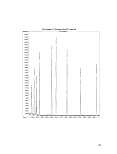 Appendix G: Cook's Distance
(Adapted from Design Expert v.7, StatEase, Inc.)
Cook's Distance (Dj) (Cook, 1977) can be thought of as a measure of the influence of an
observation (Kleinbaum et al., 1998). It is a measure of how much the regression would
change if a case is omitted from the analysis. Relatively large Dj values are associated with
cases with high leverage and large studentized residuals. These large Dj values relative to
the other cases may be an outlier and should be further investigated to determine if there is
a reason the outlier exists. A large Dj could be caused by recording errors, an incorrect
model, or a design point far from the remaining cases.
Cook's Distance is a product of the square of the /th internally studentized residual, r/, and
a monotonic function of the leverage, /?„:
Note: DI is undefined for leverages of one.
The size of Dj is determined by:
The (internally) studentized residual is: r.t = •
\\-hu
c y It
1 . The size of r;, a random variable in part reflecting the lack-of-fit to the model at the /th
case.
2. The leverage, hjj, reflecting the location of the /th experiment in the independent variable
space.
3. p is the number of model parameters (including the intercept)
A large value of D; may be due to a large TJ, a large hjj, or both.
Cook's Distance may also be interpreted as the average squared difference between the
predictions that result from the full data set and those that result from a reduced data set
(deleting the /th observation) compared to the error mean squared of the fitted model. It
can be shown that:
D =
ps2
106
image:
Appendix G: Cook's Distance
(Adapted from Design Expert v.7, StatEase, Inc.)
Cook's Distance (Dj) (Cook, 1977) can be thought of as a measure of the influence of an
observation (Kleinbaum et al., 1998). It is a measure of how much the regression would
change if a case is omitted from the analysis. Relatively large Dj values are associated with
cases with high leverage and large studentized residuals. These large Dj values relative to
the other cases may be an outlier and should be further investigated to determine if there is
a reason the outlier exists. A large Dj could be caused by recording errors, an incorrect
model, or a design point far from the remaining cases.
Cook's Distance is a product of the square of the /th internally studentized residual, r/, and
a monotonic function of the leverage, /?„:
Note: DI is undefined for leverages of one.
The size of Dj is determined by:
The (internally) studentized residual is: r.t = •
\\-hu
c y It
1 . The size of r;, a random variable in part reflecting the lack-of-fit to the model at the /th
case.
2. The leverage, hjj, reflecting the location of the /th experiment in the independent variable
space.
3. p is the number of model parameters (including the intercept)
A large value of D; may be due to a large TJ, a large hjj, or both.
Cook's Distance may also be interpreted as the average squared difference between the
predictions that result from the full data set and those that result from a reduced data set
(deleting the /th observation) compared to the error mean squared of the fitted model. It
can be shown that:
D =
ps2
106
image:
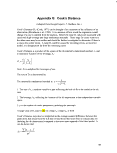 This A is also undefined for leverages of one.
An equivalent interpretation of D; is that it is a standardized weighted distance between the
vector of regression parameters obtained from the full model and the vector obtained after
deleting the /th case. If the value of Dj is substantially less than 1, then deleting the rth case
will not significantly change the estimates of the regression coefficients.
Note: The magnitude o/A is judged against the 50% point of the Fmodeidf, residual df
distribution for limits. If the F-distributions at the 50% point is approximately 1, then, a Dj
= 1 will move the estimate of the regression parameters to the edge of a 50% confidence
region, a potentially important shift. IfDi is much less than one, then deletion of that case
will not substantially shift the estimates of the regression parameters (Stat-Ease, 2006;
Weisberg, 1985).
Rather than using 1 as a cutoff rule, StatEase, Inc. suggests that all of the D, values be
examined. A plot of Cook's Distance versus the run order can be used to identify
experiments with Dj values that stand out from the rest of the runs.
In a perfectly balanced orthogonal array, Cook's Distance and the externally studentized
residual are directly related and thus give related information. In general regression
problems, there can be considerable differences in the information contained in the two
statistics; in other words, different runs may be identified for further investigation (Stat-
Ease, 2006).
References Cited
Cook, R.D., 1977, Detection of Influential Observations in Linear Regression, p. 15-18.
Kleinbaum, D.G., Kupper, L.L., Muller K.E., and Nizam, A., 1998, Applied Regression
Analysis and Multivariable Methods: Duxbury Press, p. 1-798.
Stat-Ease, I., 2006, Design-Expert 7, www.statease.com.
Weisberg, S., 1985, Applied Linear Regression: John Wiley & Sons, Inc.
107
image:
This A is also undefined for leverages of one.
An equivalent interpretation of D; is that it is a standardized weighted distance between the
vector of regression parameters obtained from the full model and the vector obtained after
deleting the /th case. If the value of Dj is substantially less than 1, then deleting the rth case
will not significantly change the estimates of the regression coefficients.
Note: The magnitude o/A is judged against the 50% point of the Fmodeidf, residual df
distribution for limits. If the F-distributions at the 50% point is approximately 1, then, a Dj
= 1 will move the estimate of the regression parameters to the edge of a 50% confidence
region, a potentially important shift. IfDi is much less than one, then deletion of that case
will not substantially shift the estimates of the regression parameters (Stat-Ease, 2006;
Weisberg, 1985).
Rather than using 1 as a cutoff rule, StatEase, Inc. suggests that all of the D, values be
examined. A plot of Cook's Distance versus the run order can be used to identify
experiments with Dj values that stand out from the rest of the runs.
In a perfectly balanced orthogonal array, Cook's Distance and the externally studentized
residual are directly related and thus give related information. In general regression
problems, there can be considerable differences in the information contained in the two
statistics; in other words, different runs may be identified for further investigation (Stat-
Ease, 2006).
References Cited
Cook, R.D., 1977, Detection of Influential Observations in Linear Regression, p. 15-18.
Kleinbaum, D.G., Kupper, L.L., Muller K.E., and Nizam, A., 1998, Applied Regression
Analysis and Multivariable Methods: Duxbury Press, p. 1-798.
Stat-Ease, I., 2006, Design-Expert 7, www.statease.com.
Weisberg, S., 1985, Applied Linear Regression: John Wiley & Sons, Inc.
107
image:
 Appendix H: Glossary of Terms and Equations
(most terms are adapted from Stat-Ease, Inc., 2006)
Adequate Precision: A signal-to-noise ratio. It compares the range of the predicted values
at the design points to the average prediction error. Ratios greater than four indicate
adequate model discrimination.
max(Y)-min(Y)
>4
£
p = number of model parameters (including intercept (bo) and any block coefficients)
CT2 = residual MS from ANOVA table
n = number of experiments
Adi. R-Squared: Adjusted R-squared, a measure of the amount of variation around the
mean explained by the model, adjusted for the number of terms in the model. The adjusted
R-squared decreases as the number of terms in the model increases if those additional terms
do not add value to the model.
residual
dfresidual
mode/
ANOVA Output: the output from the Analysis of Variance. The ANOVA is built entirely
on the premise that the factors are fixed, not random, and the design is crossed, not nested.
Blocking: Removes any variation attributed to the blocks prior to computing the ANOVA
for the factor effects by aliasing the block usually with a higher-ordered effect.
C.V.: Coefficient of Variation, the standard deviation (Std. Dev.) expressed as a
percentage of the mean. It is calculated by dividing the Std. Dev. by the mean and
multiplying by 100.
Cor. Total: corrected total, totals of all information corrected for the mean. This is
included in the ANOVA output.
Curvature: (2-level Factorials Only) Compares the average response of the factorial
points to the average response of the center points to test for non-linearity between the
factorial points.
108
image:
Appendix H: Glossary of Terms and Equations
(most terms are adapted from Stat-Ease, Inc., 2006)
Adequate Precision: A signal-to-noise ratio. It compares the range of the predicted values
at the design points to the average prediction error. Ratios greater than four indicate
adequate model discrimination.
max(Y)-min(Y)
>4
£
p = number of model parameters (including intercept (bo) and any block coefficients)
CT2 = residual MS from ANOVA table
n = number of experiments
Adi. R-Squared: Adjusted R-squared, a measure of the amount of variation around the
mean explained by the model, adjusted for the number of terms in the model. The adjusted
R-squared decreases as the number of terms in the model increases if those additional terms
do not add value to the model.
residual
dfresidual
mode/
ANOVA Output: the output from the Analysis of Variance. The ANOVA is built entirely
on the premise that the factors are fixed, not random, and the design is crossed, not nested.
Blocking: Removes any variation attributed to the blocks prior to computing the ANOVA
for the factor effects by aliasing the block usually with a higher-ordered effect.
C.V.: Coefficient of Variation, the standard deviation (Std. Dev.) expressed as a
percentage of the mean. It is calculated by dividing the Std. Dev. by the mean and
multiplying by 100.
Cor. Total: corrected total, totals of all information corrected for the mean. This is
included in the ANOVA output.
Curvature: (2-level Factorials Only) Compares the average response of the factorial
points to the average response of the center points to test for non-linearity between the
factorial points.
108
image:
 DFFITS: difference in fits, is a measure of the amount of influence the ith observation has
on the predicted value. Lower values are better. Points which exceed the limits should be
further investigated. DFFITS is calculated by measuring the change in the predicted values
that occurs when the response value is deleted. The larger the value, the more it influences
the fitted model.
DF: Degrees of freedom when attributed to the blocks, is generally equal to one less than
the number of blocks. DF for the model is the number of model terms, including the
intercept, minus one. DF for the term is the number of levels for the term, minus one. DF
may also represent the amount of information used up to estimate curvature, or the
corrected total DF minus the model DF, the amount of information available after
accounting for blocking, model terms, curvature, and purely experimental uncertainty, the
amount of information available from replicated points, or the total degrees-of-freedom for
the experiment, minus one for the mean.
F Value: Test for comparing model, term, curvature, or lack-of-fit variance with residual
(error) variance. If the variances are close to the same, then the ratio will be close to one
and it is less likely that any of the factors, curvature, or lack-of-fit have a significant effect
on the response. F-value is calculated by dividing the model, term, curvature, or lack-of-fit
variance mean square by the residual mean square.
Lack-of-Fit (LOF): LOF is the variation of the data around the fitted model. If the model
does not fit the data well, then this will be significant.
Leverage: Leverage is the potential for a value to influence the fit of the model
parameters. It is a numerical value ranging from zero to one. Leverages at or near one
should be avoided as this indicates a problem with the data point that error strongly
influences the model.
Mean: Overall average of the response data.
Mean Square of the Block: Estimate of the block variance, calculated by the block sum
of squares divided by block degrees-of-freedom.
Mean Square of the Curvature: Estimate of the curvature variance, calculated by the
curvature sum of squares divided by curvature degrees of freedom.
Mean Square of the Process: Estimate of process variance. The square root of this
provides an estimate of the process standard deviation.
Mean Square of the Lack-of-Fit: Estimate of the. lack-of-fit.
Mean Square of the Error: Estimate of the purely experimental variance.
Mean Square of the Model: Estimate of the model variance, calculated by the model sum
of squares divided by the model degrees of freedom.
109
image:
DFFITS: difference in fits, is a measure of the amount of influence the ith observation has
on the predicted value. Lower values are better. Points which exceed the limits should be
further investigated. DFFITS is calculated by measuring the change in the predicted values
that occurs when the response value is deleted. The larger the value, the more it influences
the fitted model.
DF: Degrees of freedom when attributed to the blocks, is generally equal to one less than
the number of blocks. DF for the model is the number of model terms, including the
intercept, minus one. DF for the term is the number of levels for the term, minus one. DF
may also represent the amount of information used up to estimate curvature, or the
corrected total DF minus the model DF, the amount of information available after
accounting for blocking, model terms, curvature, and purely experimental uncertainty, the
amount of information available from replicated points, or the total degrees-of-freedom for
the experiment, minus one for the mean.
F Value: Test for comparing model, term, curvature, or lack-of-fit variance with residual
(error) variance. If the variances are close to the same, then the ratio will be close to one
and it is less likely that any of the factors, curvature, or lack-of-fit have a significant effect
on the response. F-value is calculated by dividing the model, term, curvature, or lack-of-fit
variance mean square by the residual mean square.
Lack-of-Fit (LOF): LOF is the variation of the data around the fitted model. If the model
does not fit the data well, then this will be significant.
Leverage: Leverage is the potential for a value to influence the fit of the model
parameters. It is a numerical value ranging from zero to one. Leverages at or near one
should be avoided as this indicates a problem with the data point that error strongly
influences the model.
Mean: Overall average of the response data.
Mean Square of the Block: Estimate of the block variance, calculated by the block sum
of squares divided by block degrees-of-freedom.
Mean Square of the Curvature: Estimate of the curvature variance, calculated by the
curvature sum of squares divided by curvature degrees of freedom.
Mean Square of the Process: Estimate of process variance. The square root of this
provides an estimate of the process standard deviation.
Mean Square of the Lack-of-Fit: Estimate of the. lack-of-fit.
Mean Square of the Error: Estimate of the purely experimental variance.
Mean Square of the Model: Estimate of the model variance, calculated by the model sum
of squares divided by the model degrees of freedom.
109
image:
 Model: Terms estimating the parameters. For 2-level factorials, those that "fall off the
normal probability line of the effects plot. A model is a response given as a function of
factors. A regression model estimates the effects (parameters) of the factors on the
response. The model may be deterministic or stochastic (probabilistic)
Fred. R-Squared: A measure of the amount of variation in new data explained by the
model.
Pred2=l-
PRESS
residualmodel
= 1-
PRESS
'total ""curvature ""block
The predicted R-squared and the adjusted R-squared should be within 0.20 of each other.
PRESS: Predicted Residual Error Sum of Squares is a measure of how the model fits each
point in the design. The PRESS is computed by first predicting where each point should be
from a model that contains all of the other points except the one in question. The squared •
residuals (difference between actual and predicted values) are then summed.
6- . = V- — V- •
I,-I J I •'I,-I
PRESS =
Prob > F: Probability of seeing the observed F value if the null hypothesis is true (e.g.,
there is no factor effect or there is no curvature). Small probability values call for rejection
of the null hypothesis. The probability equals the proportion of the area under the curve of
the F-distribution that lies beyond the observed F value. The F-distribution itself is
determined by the degrees of freedom associated with the variances being compared.
(In other words, if the Prob>F value is very small (less than 0.05) then the terms in the
model have a significant effect on the response, or the curvature is significant. This means
that the predicted value at the center point is significantly different than the value that is
obtained when actually running the center point conditions. Generally the Prob>F value
for curvature should be greater than 0.10. (Stat-Ease Inc., 2006))
Purely Experimental Uncertainty: Amount of variation in the response in replicated
design points.
R-Squared: A measure of the amount of variation around the mean explained by the
model.
110
image:
Model: Terms estimating the parameters. For 2-level factorials, those that "fall off the
normal probability line of the effects plot. A model is a response given as a function of
factors. A regression model estimates the effects (parameters) of the factors on the
response. The model may be deterministic or stochastic (probabilistic)
Fred. R-Squared: A measure of the amount of variation in new data explained by the
model.
Pred2=l-
PRESS
residualmodel
= 1-
PRESS
'total ""curvature ""block
The predicted R-squared and the adjusted R-squared should be within 0.20 of each other.
PRESS: Predicted Residual Error Sum of Squares is a measure of how the model fits each
point in the design. The PRESS is computed by first predicting where each point should be
from a model that contains all of the other points except the one in question. The squared •
residuals (difference between actual and predicted values) are then summed.
6- . = V- — V- •
I,-I J I •'I,-I
PRESS =
Prob > F: Probability of seeing the observed F value if the null hypothesis is true (e.g.,
there is no factor effect or there is no curvature). Small probability values call for rejection
of the null hypothesis. The probability equals the proportion of the area under the curve of
the F-distribution that lies beyond the observed F value. The F-distribution itself is
determined by the degrees of freedom associated with the variances being compared.
(In other words, if the Prob>F value is very small (less than 0.05) then the terms in the
model have a significant effect on the response, or the curvature is significant. This means
that the predicted value at the center point is significantly different than the value that is
obtained when actually running the center point conditions. Generally the Prob>F value
for curvature should be greater than 0.10. (Stat-Ease Inc., 2006))
Purely Experimental Uncertainty: Amount of variation in the response in replicated
design points.
R-Squared: A measure of the amount of variation around the mean explained by the
model.
110
image:
 R2=l-
SS.
residual
residual +^mqde/J
= 1-
residual
total curvature block
Residual: Consists of terms used to estimate experimental error (for 2-level factorials, the
insignificant factors and interactions that fall on the normal probability line on the effects
plot.)
Std Dev: Square root of a mean square or variance of the sum-of-squares divided by the
degrees-of- freedom. The square root of the mean sum-of-squares of the purely
experimental uncertainty may be considered an estimate of the standard deviation
associated with the experiment.
Sum of Squares: The transpose of a matrix times that matrix. In regression ANOVA the
sum-of-squares of the responses is portioned into various sums-of-squares to determine the
significance of model factors over residuals.
The ANOVA can be calculated using either partial sums of squares, sequential sums of
squares, or a classical sum of squares (Stat-Ease Inc., 2006).
VIF: is the variance inflation factor and indicates how much the variance of that model
coefficient increases due to the lack of orthogonality in the design. The standard error of a
model coefficient increases in proportion to the square root of the VIF. If a coefficient is
orthogonal to the remaining model terms, the VIF is one. One or more large VIFs indicate
multicollinearity. VIFs exceeding ten indicate problems due to multicollinearity. (For
example, if a coefficient has a VIF of 16, its standard error is 4 times as large as it would be
in an orthogonal design.) The VIF is related to R;2 by the following:
Ri2 is the multiple correlation coefficient (also known as the coefficient of determination)
and is calculated by regressing the factor in question on all other factors. Considering the
factor in question (Xf) as Y: Rj2 = (SYY - RSS)/SYY where SYY is the sum-of-squares
corrected for the mean of Xi and RSS is the sum of squares residuals regressing Xj on all
other factors. If the design is orthogonal these two sums of squares are equal and Rj2 is
zero. Since the VIF = !/(!- Rj2), when Rj2 is zero, the VIF is one. If the design is not
orthogonal the quantity (SYY - RSS) is not zero and represents the variation in Xj that can
be explained by the settings of the other factors. It is a measure of the collinearity of Xj
with the other X's (Stat-Ease, 2006).
Ill
image:
R2=l-
SS.
residual
residual +^mqde/J
= 1-
residual
total curvature block
Residual: Consists of terms used to estimate experimental error (for 2-level factorials, the
insignificant factors and interactions that fall on the normal probability line on the effects
plot.)
Std Dev: Square root of a mean square or variance of the sum-of-squares divided by the
degrees-of- freedom. The square root of the mean sum-of-squares of the purely
experimental uncertainty may be considered an estimate of the standard deviation
associated with the experiment.
Sum of Squares: The transpose of a matrix times that matrix. In regression ANOVA the
sum-of-squares of the responses is portioned into various sums-of-squares to determine the
significance of model factors over residuals.
The ANOVA can be calculated using either partial sums of squares, sequential sums of
squares, or a classical sum of squares (Stat-Ease Inc., 2006).
VIF: is the variance inflation factor and indicates how much the variance of that model
coefficient increases due to the lack of orthogonality in the design. The standard error of a
model coefficient increases in proportion to the square root of the VIF. If a coefficient is
orthogonal to the remaining model terms, the VIF is one. One or more large VIFs indicate
multicollinearity. VIFs exceeding ten indicate problems due to multicollinearity. (For
example, if a coefficient has a VIF of 16, its standard error is 4 times as large as it would be
in an orthogonal design.) The VIF is related to R;2 by the following:
Ri2 is the multiple correlation coefficient (also known as the coefficient of determination)
and is calculated by regressing the factor in question on all other factors. Considering the
factor in question (Xf) as Y: Rj2 = (SYY - RSS)/SYY where SYY is the sum-of-squares
corrected for the mean of Xi and RSS is the sum of squares residuals regressing Xj on all
other factors. If the design is orthogonal these two sums of squares are equal and Rj2 is
zero. Since the VIF = !/(!- Rj2), when Rj2 is zero, the VIF is one. If the design is not
orthogonal the quantity (SYY - RSS) is not zero and represents the variation in Xj that can
be explained by the settings of the other factors. It is a measure of the collinearity of Xj
with the other X's (Stat-Ease, 2006).
Ill
image:
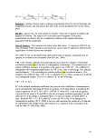 References Cited
Stat-Ease Inc., 2006, Design-Expert 7.
Stat-Ease, I., 2006, Design-Expert 7, www.statease.com.
112
image:
References Cited
Stat-Ease Inc., 2006, Design-Expert 7.
Stat-Ease, I., 2006, Design-Expert 7, www.statease.com.
112
image:
 Appendix I: Oil-Red-O Molecular Structure
3 eMolcculcs Molecule Details - Microsoft Internet Explorer
SMILES: Cclc(ccc(/N=N/c2c(O)ccc3ccccc23)clC)/N=N/clcccc(C)cl C
CAS: 1320-06-5
NAME: Oil Red O
GYI
Close this window
© 2007 eMolecules Inc.
c Molecules*
Adapted from: http://www.emolecules.com/cgi-bin/search?t=ex&q=l 320-06-5
113
image:
Appendix I: Oil-Red-O Molecular Structure
3 eMolcculcs Molecule Details - Microsoft Internet Explorer
SMILES: Cclc(ccc(/N=N/c2c(O)ccc3ccccc23)clC)/N=N/clcccc(C)cl C
CAS: 1320-06-5
NAME: Oil Red O
GYI
Close this window
© 2007 eMolecules Inc.
c Molecules*
Adapted from: http://www.emolecules.com/cgi-bin/search?t=ex&q=l 320-06-5
113
image:
 Appendix J: Brilliant Blue G-250 Molecular Structure
eMolecules Molecule Details - Microsoft Internet Explorer
Na"
SMILES:
[Na+]. CCOcl ccc(ccl )Ncl ccc(ccl )/C(=C 1/C=C/C( = [N+](/CC)\Cc2cccc(c2)S(=O)(=O)
[0-])\C=C\lC)\clccc(cclC)N(CC)Cclccc(ccl)S(=O)(=O)[0-]
CAS: 6104-58-1 Q Yj.
NAME: COOMASSIE BRILLIANT BLUE G-250 (C.I. 42655) BIOLOGICAL STAIN £ YJ.
Close this window
g> 2007 eMolecules Inc.
c Molecules*
Adapted from: http://www.emolecules.com/cgi-bin/search?t=ex&q=6104-58-l
114
image:
Appendix J: Brilliant Blue G-250 Molecular Structure
eMolecules Molecule Details - Microsoft Internet Explorer
Na"
SMILES:
[Na+]. CCOcl ccc(ccl )Ncl ccc(ccl )/C(=C 1/C=C/C( = [N+](/CC)\Cc2cccc(c2)S(=O)(=O)
[0-])\C=C\lC)\clccc(cclC)N(CC)Cclccc(ccl)S(=O)(=O)[0-]
CAS: 6104-58-1 Q Yj.
NAME: COOMASSIE BRILLIANT BLUE G-250 (C.I. 42655) BIOLOGICAL STAIN £ YJ.
Close this window
g> 2007 eMolecules Inc.
c Molecules*
Adapted from: http://www.emolecules.com/cgi-bin/search?t=ex&q=6104-58-l
114
image:
 Appendix K: Experimental Factor Properties
Experimental
Treatment
4% Tween 80
4% Tween 80 + 10%
EtOH
50 mM Tween 60
0.5% AMA-80-I
8% AMA-80-I
0.025% Steol CS-330
0.10% Steol CS-330
0.5% Dowfax 8390
5% Dowfax 8390
Oil-Red-O Dye
Brilliant Blue Dye
(COOMASSffi
Brilliant Blue G-250)
PCE
Molecular
Wt
g/mol
1310
1356
1312
388
388
421
421
643 (ave)
643 (ave)
409
854
166
Chemical Formula
C(S4Hi24O26
CwHi^OisQHjOH
C^KI^OM
C16H29O7NaS
CI6H2907NaS
CH3(CH2)10CH2(OCH2CH2)30S03Na
CH3(CH2)K,CH2(OCH2CH2)3OSOjNa
Proprietary; Alkyldiphenyloxide Disulfate
Proprietary; Alkyldiphenyloxide Disulfate
CasH^O
C47H49N3O7S2Na
C2CL, (C12C=CC12)
CAS#
9005-65-6
9005-65-6 +
EtOH
9005-67-8
002373-38-8
9004-82-4
9004-82-4
Unknown
unknown
1320-06-5
6104-58-1
127-18-4
Critical Micelle
Concentration
0.012mM
449mg/L
449mg/L
0.014 g/lOOg in 0.1
MNaCl
Charge
Nonionic
Nonionic
Nonionic
Anionic
Anionic
Anionic
Anionic
Anionic
Anionic
image:
Appendix K: Experimental Factor Properties
Experimental
Treatment
4% Tween 80
4% Tween 80 + 10%
EtOH
50 mM Tween 60
0.5% AMA-80-I
8% AMA-80-I
0.025% Steol CS-330
0.10% Steol CS-330
0.5% Dowfax 8390
5% Dowfax 8390
Oil-Red-O Dye
Brilliant Blue Dye
(COOMASSffi
Brilliant Blue G-250)
PCE
Molecular
Wt
g/mol
1310
1356
1312
388
388
421
421
643 (ave)
643 (ave)
409
854
166
Chemical Formula
C(S4Hi24O26
CwHi^OisQHjOH
C^KI^OM
C16H29O7NaS
CI6H2907NaS
CH3(CH2)10CH2(OCH2CH2)30S03Na
CH3(CH2)K,CH2(OCH2CH2)3OSOjNa
Proprietary; Alkyldiphenyloxide Disulfate
Proprietary; Alkyldiphenyloxide Disulfate
CasH^O
C47H49N3O7S2Na
C2CL, (C12C=CC12)
CAS#
9005-65-6
9005-65-6 +
EtOH
9005-67-8
002373-38-8
9004-82-4
9004-82-4
Unknown
unknown
1320-06-5
6104-58-1
127-18-4
Critical Micelle
Concentration
0.012mM
449mg/L
449mg/L
0.014 g/lOOg in 0.1
MNaCl
Charge
Nonionic
Nonionic
Nonionic
Anionic
Anionic
Anionic
Anionic
Anionic
Anionic
image: