<pubnumber>420P07003</pubnumber>
<title>SmartWay Fuel Efficiency Test Protocol for Medium and Heavy Duty Vehicles: Working Draft</title>
<pages>76</pages>
<pubyear>2007</pubyear>
<provider>NEPIS</provider>
<access>online</access>
<origin>PDF</origin>
<author></author>
<publisher></publisher>
<subject></subject>
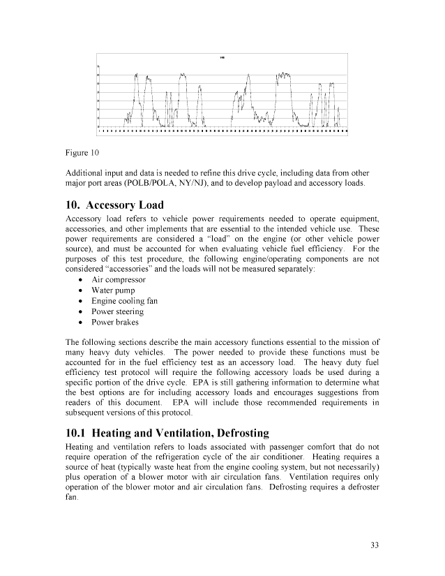
<abstract></abstract>
<operator>mja</operator>
<scandate>12/16/08</scandate>
<type>single page tiff</type>
<keyword></keyword>
Smart Way Fuel Efficiency Test Protocol
for Medium and Heavy Duty Vehicles
Working Draft
United States
Environmental Protection
Agency
image:
 Smart Way Fuel Efficiency Test Protocol
for Medium and Heavy Duty Vehicles
Working Draft
Transportation and Regional Programs Division
Office of Transportation and Air Quality
U.S. Environmental Protection Agency
v>EPA
NOTICE
This technical report does not necessarily represent final EPA decisions or
positions. It is intended to present technical analysis of issues using data
that are currently available. The purpose in the release of such reports is to
facilitate the exchange of technical information and to inform the public of
technical developments.
United States EPA420-P-07-003
Environmental Protection ., , „„.,
Agency November 2007
image:
Smart Way Fuel Efficiency Test Protocol
for Medium and Heavy Duty Vehicles
Working Draft
Transportation and Regional Programs Division
Office of Transportation and Air Quality
U.S. Environmental Protection Agency
v>EPA
NOTICE
This technical report does not necessarily represent final EPA decisions or
positions. It is intended to present technical analysis of issues using data
that are currently available. The purpose in the release of such reports is to
facilitate the exchange of technical information and to inform the public of
technical developments.
United States EPA420-P-07-003
Environmental Protection ., , „„.,
Agency November 2007
image:
 Table of Contents
1. Foreword 5
2. Purpose and Scope 6
3. Overview of Test Methods 9
3.1 Track Test 10
3.2 Chassis Dynamometer Test 12
4. Vehicle Selection 13
5. Test Fuel 14
6. Test Track Specifications and Requirements 15
6.1 Track Specifications 15
6.2 Track Requirements 16
6.3 Track Environmental Requirements 17
7. Chassis Dynamometer Specifications and Requirements 18
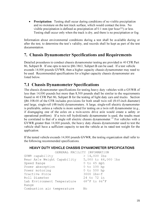
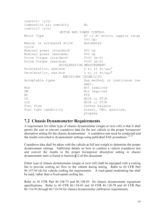
7.1 Chassis Dynamometer Specifications 18
7.2 Chassis Dynamometer Requirements 19
7.3 Chassis Dynamometer Environmental Requirements 20
8. Test Equipment Specifications 20
8.1 Laboratory Emissions Monitoring System 20
8.2 Portable Emissions Monitoring Measurement System 21
8.3 Gravimetric Fuel Consumption Measurement System 21
9. Drive Cycle Selection 22
9.1 Drive Cycle Selection Criteria 22
9.2 Highway Line Haul 23
9.3 Regional Haul 25
9.4 Local Pick Up and Delivery 25
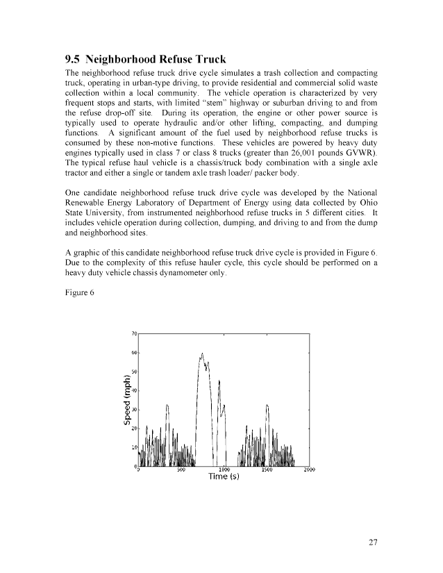
9.5 Neighborhood Refuse Truck 27
9.6 Utility Service Truck 28
9.7 Transit Bus 29
9.8 Intermodal Drayage Truck 32
10. Accessory Load 33
10.1 Heating and Ventilation, Defrosting 33
10.2 Air Conditioning 34
10.3 Power Take-off (PTO) or Other Vocational/Service Work Load 34
10.4 Lamps and Lights 34
10.5 Miscellaneous 34
10.6 Drive Cycle Load Requirements 34
11. Vehicle Payload and Test Weight 35
11.1 Test Equivalent Weight 37
11.2 Test Fuel Weight and Volume 37
12. Test Set-Up Procedure 38
12.1 Test Payload 38
12.2 Tire Pressure 38
12.3 Mechanical Preparation of Test Vehicle 38
12.4 Vehicle Preconditioning 39
12.5 Hybrid Vehicles - Additional Vehicle Conditioning 40
12.6 Hybrid Vehicles - Procedures for Determining State of Charge (SOC) and Net Energy
Change (NEC) 41
12.7 Fuel Analysis 43
13. Test Procedure 43
image:
Table of Contents
1. Foreword 5
2. Purpose and Scope 6
3. Overview of Test Methods 9
3.1 Track Test 10
3.2 Chassis Dynamometer Test 12
4. Vehicle Selection 13
5. Test Fuel 14
6. Test Track Specifications and Requirements 15
6.1 Track Specifications 15
6.2 Track Requirements 16
6.3 Track Environmental Requirements 17
7. Chassis Dynamometer Specifications and Requirements 18
7.1 Chassis Dynamometer Specifications 18
7.2 Chassis Dynamometer Requirements 19
7.3 Chassis Dynamometer Environmental Requirements 20
8. Test Equipment Specifications 20
8.1 Laboratory Emissions Monitoring System 20
8.2 Portable Emissions Monitoring Measurement System 21
8.3 Gravimetric Fuel Consumption Measurement System 21
9. Drive Cycle Selection 22
9.1 Drive Cycle Selection Criteria 22
9.2 Highway Line Haul 23
9.3 Regional Haul 25
9.4 Local Pick Up and Delivery 25
9.5 Neighborhood Refuse Truck 27
9.6 Utility Service Truck 28
9.7 Transit Bus 29
9.8 Intermodal Drayage Truck 32
10. Accessory Load 33
10.1 Heating and Ventilation, Defrosting 33
10.2 Air Conditioning 34
10.3 Power Take-off (PTO) or Other Vocational/Service Work Load 34
10.4 Lamps and Lights 34
10.5 Miscellaneous 34
10.6 Drive Cycle Load Requirements 34
11. Vehicle Payload and Test Weight 35
11.1 Test Equivalent Weight 37
11.2 Test Fuel Weight and Volume 37
12. Test Set-Up Procedure 38
12.1 Test Payload 38
12.2 Tire Pressure 38
12.3 Mechanical Preparation of Test Vehicle 38
12.4 Vehicle Preconditioning 39
12.5 Hybrid Vehicles - Additional Vehicle Conditioning 40
12.6 Hybrid Vehicles - Procedures for Determining State of Charge (SOC) and Net Energy
Change (NEC) 41
12.7 Fuel Analysis 43
13. Test Procedure 43
image:
 13.1 General Requirements 43
Driver Conduct 43
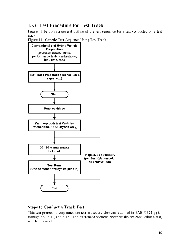
13.2 Test Procedure for Test Track 46
13.3 Test Procedure for Chassis Dynamometer 47
13.4 Coastdown Test Procedure to Calculate Road Load 49
14 Required Number of Test Runs 50
14.1 General Requirements 50
14.2 Number of Test Runs for Test Track Test 51
14.3 Number of Test Runs for Chassis Dynamometer Test 52
15 Fuel efficiency Calculation 54
16 Reporting and Documentation 55
16.1 Reports 55
16.2 Data and Metrics 56
16.3 Quality Assurance and Control 56
16.4 Assessment 57
17 Appendices 58
17.1 Appendix A 59
17.2 - 17.8 Appendices B - H 61
17.9 Appendix I 62
17.11 Appendix K 71
image:
13.1 General Requirements 43
Driver Conduct 43
13.2 Test Procedure for Test Track 46
13.3 Test Procedure for Chassis Dynamometer 47
13.4 Coastdown Test Procedure to Calculate Road Load 49
14 Required Number of Test Runs 50
14.1 General Requirements 50
14.2 Number of Test Runs for Test Track Test 51
14.3 Number of Test Runs for Chassis Dynamometer Test 52
15 Fuel efficiency Calculation 54
16 Reporting and Documentation 55
16.1 Reports 55
16.2 Data and Metrics 56
16.3 Quality Assurance and Control 56
16.4 Assessment 57
17 Appendices 58
17.1 Appendix A 59
17.2 - 17.8 Appendices B - H 61
17.9 Appendix I 62
17.11 Appendix K 71
image:
 List of Figures and Tables
[Reserved]
image:
List of Figures and Tables
[Reserved]
image:
 1. Foreword
Advancements in heavy duty vehicle technology offer the potential for significant
improvements in important vehicle attributes, including efficiency and emissions
performance. In 2004, the U.S. Environmental Protection Agency (EPA) initiated the
SmartWaySM Transport Partnership to accelerate the deployment of fuel-efficient, clean
technologies for heavy duty vehicles. SmartWay Transport is an innovative collaboration
between EPA and the transportation industry to improve energy efficiency, reduce
greenhouse gas and air pollutant emissions, and improve energy security. Through
SmartWay, EPA works in collaboration with industry and other stakeholders to provide
incentives for adopting cleaner, more fuel efficient transportation technologies to benefit
the environment.
An important aspect of the SmartWay Transport Partnership is to determine through
testing and analysis the environmental benefits of heavy truck technologies, and to
provide this information to SmartWay partners and to the general public. SmartWay is
developing this fuel efficiency test protocol for heavy duty trucks to better quantify the
benefits of various heavy vehicle designs and technologies. EPA currently offers a
"SmartWay designation" for over-the-road tractor-trailer combination trucks. It is a
design-based specification, developed on this basis of test results for individual
components (tires, wheels, aerodynamic equipment, auxiliary power units, engines) that
have been demonstrated to improve fuel efficiency and reduce emissions. EPA, its
SmartWay partners, and others would like to expand the SmartWay designation for heavy
duty vehicles by moving toward a performance-based specification. A performance-
based specification would be technology-neutral, and able to quantify a broad range of
heavy vehicle configurations and applications, and to measure technical innovations as
they emerge.
Moving toward a performance-based specification requires using a test to measure
vehicle fuel efficiency. Component testing alone is not sufficient, since the fuel-saving
impacts can vary widely based upon vehicle application. However, a standardized,
objective, stand-alone fuel efficiency test to measure the fuel efficiency of a heavy duty
on-highway vehicle does not currently exist. This absence presents a significant
challenge to SmartWay, the Agency and industry. Without a test method, it is difficult to
develop a common understanding of how to assess and compare the fuel efficiency of
heavy duty vehicles, including vehicles with hybrid powertrain, varying aerodynamic
configurations, and other advanced vehicle designs. EPA recognizes that there is a wide
variety of truck configurations for each base model and that it may not be possible to test
every configuration to see if it meets the SmartWay performance specification. As a
result, EPA is looking at methods to extend fuel efficiency testing to cover additional
truck configurations. Tools such as the consistent use of vehicle modeling, tire rolling
resistance testing, and aerodynamic evaluations could potentially broaden a fuel
efficiency testing program.
This test procedure applies to medium and heavy duty vehicles as per 40 CFR §86.082-2.
This means any motor vehicle rated at more than 8,500 pounds GVWR or that has a
image:
1. Foreword
Advancements in heavy duty vehicle technology offer the potential for significant
improvements in important vehicle attributes, including efficiency and emissions
performance. In 2004, the U.S. Environmental Protection Agency (EPA) initiated the
SmartWaySM Transport Partnership to accelerate the deployment of fuel-efficient, clean
technologies for heavy duty vehicles. SmartWay Transport is an innovative collaboration
between EPA and the transportation industry to improve energy efficiency, reduce
greenhouse gas and air pollutant emissions, and improve energy security. Through
SmartWay, EPA works in collaboration with industry and other stakeholders to provide
incentives for adopting cleaner, more fuel efficient transportation technologies to benefit
the environment.
An important aspect of the SmartWay Transport Partnership is to determine through
testing and analysis the environmental benefits of heavy truck technologies, and to
provide this information to SmartWay partners and to the general public. SmartWay is
developing this fuel efficiency test protocol for heavy duty trucks to better quantify the
benefits of various heavy vehicle designs and technologies. EPA currently offers a
"SmartWay designation" for over-the-road tractor-trailer combination trucks. It is a
design-based specification, developed on this basis of test results for individual
components (tires, wheels, aerodynamic equipment, auxiliary power units, engines) that
have been demonstrated to improve fuel efficiency and reduce emissions. EPA, its
SmartWay partners, and others would like to expand the SmartWay designation for heavy
duty vehicles by moving toward a performance-based specification. A performance-
based specification would be technology-neutral, and able to quantify a broad range of
heavy vehicle configurations and applications, and to measure technical innovations as
they emerge.
Moving toward a performance-based specification requires using a test to measure
vehicle fuel efficiency. Component testing alone is not sufficient, since the fuel-saving
impacts can vary widely based upon vehicle application. However, a standardized,
objective, stand-alone fuel efficiency test to measure the fuel efficiency of a heavy duty
on-highway vehicle does not currently exist. This absence presents a significant
challenge to SmartWay, the Agency and industry. Without a test method, it is difficult to
develop a common understanding of how to assess and compare the fuel efficiency of
heavy duty vehicles, including vehicles with hybrid powertrain, varying aerodynamic
configurations, and other advanced vehicle designs. EPA recognizes that there is a wide
variety of truck configurations for each base model and that it may not be possible to test
every configuration to see if it meets the SmartWay performance specification. As a
result, EPA is looking at methods to extend fuel efficiency testing to cover additional
truck configurations. Tools such as the consistent use of vehicle modeling, tire rolling
resistance testing, and aerodynamic evaluations could potentially broaden a fuel
efficiency testing program.
This test procedure applies to medium and heavy duty vehicles as per 40 CFR §86.082-2.
This means any motor vehicle rated at more than 8,500 pounds GVWR or that has a
image:
 vehicle curb weight of more than 6,000 pounds or that has a basic vehicle frontal area in
excess of 45 square feet. Vehicles in this group are typically tractor-trailer combination
trucks, single unit commercial trucks, heavy duty vocational trucks, and buses used in
inter-city transit applications. EPA does have an optional chassis certification procedure
for heavy duty diesel vehicles under 14,000 pounds GVWR, used in federal regulatory
programs (§86.1863-07). This test procedure incorporates many aspects of the optional
chassis test procedure, but does not replace it for the purposes of certifying to the
standards specified in §86.1816-08.
Heavy duty vehicle manufacturers are required to use engines that are certified to U.S.
Environmental Protection Agency (EPA) emission standards (per 40 CFR Part 86,
Subpart N) but those test procedures measure engine (rather than vehicle) brake specific
fuel consumption performance and focus on emissions rather than fuel efficiency. The
existing tests do not quantify fuel efficiency benefits from the unique features of a hybrid
drive train (regenerative braking, reductions in engine transient operation, smaller
engines) or fuel efficient vehicle components (single wide base tires, aerodynamic
equipment.) This test procedure will serve as an objective means to evaluate these and
other emerging fuel-saving technologies, and to standardize the measurement of heavy
duty vehicle fuel efficiency.
This test procedure is intended to be used on a voluntary basis to determine whether
vehicle configurations meet or exceed SmartWay performance specifications. Other
users may also wish to apply it for their own purposes. For example, the test procedure
can be used to calibrate and verify vehicle software models, allowing for greater
consistency among models.
This protocol references various SAE standards, federal regulations, and other source
documents. Those documents should be acquired in order to conduct tests in accordance
with this protocol.
This "working draft" document contains a number of "reserved" sections. It is presented
for stakeholder review in order to assist EPA in resolving certain outstanding technical
issues contained in the "reserved" sections and elsewhere. We encourage stakeholders
and other interested parties to comment on this document and provide EPA with advice
on the technical issues.
2. Purpose and Scope
The purpose of this document is to provide a standardized, objective, consistent test
procedure to measure the fuel consumption of heavy duty vehicles used in on-road
operation. As mentioned in the Foreword, this test procedure is being developed to
support the aims of the EPA SmartWay Transport Partnership, and to fill a real need in
the trucking industry. SmartWay Transport is an innovative collaboration between EPA
and the transportation industry to improve energy efficiency, reduce greenhouse gas and
air pollutant emissions, and improve energy security. An important aspect of the
image:
vehicle curb weight of more than 6,000 pounds or that has a basic vehicle frontal area in
excess of 45 square feet. Vehicles in this group are typically tractor-trailer combination
trucks, single unit commercial trucks, heavy duty vocational trucks, and buses used in
inter-city transit applications. EPA does have an optional chassis certification procedure
for heavy duty diesel vehicles under 14,000 pounds GVWR, used in federal regulatory
programs (§86.1863-07). This test procedure incorporates many aspects of the optional
chassis test procedure, but does not replace it for the purposes of certifying to the
standards specified in §86.1816-08.
Heavy duty vehicle manufacturers are required to use engines that are certified to U.S.
Environmental Protection Agency (EPA) emission standards (per 40 CFR Part 86,
Subpart N) but those test procedures measure engine (rather than vehicle) brake specific
fuel consumption performance and focus on emissions rather than fuel efficiency. The
existing tests do not quantify fuel efficiency benefits from the unique features of a hybrid
drive train (regenerative braking, reductions in engine transient operation, smaller
engines) or fuel efficient vehicle components (single wide base tires, aerodynamic
equipment.) This test procedure will serve as an objective means to evaluate these and
other emerging fuel-saving technologies, and to standardize the measurement of heavy
duty vehicle fuel efficiency.
This test procedure is intended to be used on a voluntary basis to determine whether
vehicle configurations meet or exceed SmartWay performance specifications. Other
users may also wish to apply it for their own purposes. For example, the test procedure
can be used to calibrate and verify vehicle software models, allowing for greater
consistency among models.
This protocol references various SAE standards, federal regulations, and other source
documents. Those documents should be acquired in order to conduct tests in accordance
with this protocol.
This "working draft" document contains a number of "reserved" sections. It is presented
for stakeholder review in order to assist EPA in resolving certain outstanding technical
issues contained in the "reserved" sections and elsewhere. We encourage stakeholders
and other interested parties to comment on this document and provide EPA with advice
on the technical issues.
2. Purpose and Scope
The purpose of this document is to provide a standardized, objective, consistent test
procedure to measure the fuel consumption of heavy duty vehicles used in on-road
operation. As mentioned in the Foreword, this test procedure is being developed to
support the aims of the EPA SmartWay Transport Partnership, and to fill a real need in
the trucking industry. SmartWay Transport is an innovative collaboration between EPA
and the transportation industry to improve energy efficiency, reduce greenhouse gas and
air pollutant emissions, and improve energy security. An important aspect of the
image:
 Partnership is to determine through testing and analysis the environmental benefits of
heavy truck technologies, and to provide this information to SmartWay partners and to
the general public. SmartWay is developing this fuel efficiency test procedure for heavy
duty trucks to better quantify the benefits of various heavy vehicle designs and
technologies. This test procedure provides test requirements and methods that are
appropriate for a number of different truck types, based on the specific application or
service category of the heavy duty vehicle.
This test protocol fills a real need, since there is no widely-accepted, standardized test
procedure to measure the real-world fuel consumption performance of a heavy duty
vehicle. SAE J1321 (or alternatively, SAE J1526) has been used to partially fill this gap,
but these test methods do not measure absolute vehicle fuel efficiency, but an
improvement in fuel efficiency from a baseline condition.1 This is not useful as a stand-
alone metric, since the baseline condition is not standardized. More importantly, drive
cycles are not standardized.
The test protocol described in this document measures fuel consumption directly, and the
desired fuel consumption metric for this test procedure is fuel consumed per unit of work
performed (e.g., gallons per mile or per ton-mile; for vocational trucks with power take-
off, gallons per hour). Alternatively, the metric can be work performed per volume of
fuel consumed (e.g., miles or ton-miles per gallon). A fuel consumption rather than a
percent improvement metric allows for a stand-alone efficiency measure for any given
truck model. It also provides a consistent, objective, standardized means to compare the
fuel efficiency of two or more tested trucks.
The test procedure described here is intended to provide the federal government, states,
industry, academia, and others with an objective testing method to assess the fuel
efficiency performance of heavy duty vehicles for a variety of purposes. These purposes
may include quantifying and benchmarking in-use fuel consumption; verifying fuel
savings for federal and state incentives; demonstrating environmental performance to
achieve targets for innovative industry, federal and state programs; and, providing
quantification of carbon dioxide reductions.
A major challenge to our collective understanding of heavy truck fuel efficiency is the
lack of standardized, comparative test data. This test procedure could be used to test
several trucks at the same facility, under stable test conditions. The results could be used
to establish "environmental reference" vehicles, against which other heavy duty vehicles
could be tested in the future. Using this test procedure to establish environmental
reference trucks can provide a flexible, cost-effective means to build comparable data
sets and improve our ability to analyze and understand heavy truck performance.
This test procedure establishes uniform test conditions for the most common types of
heavy duty highway vehicles and applications. Uniform test conditions include:
• vehicle selection
• fuel specification
• test facilities and environment
image:
Partnership is to determine through testing and analysis the environmental benefits of
heavy truck technologies, and to provide this information to SmartWay partners and to
the general public. SmartWay is developing this fuel efficiency test procedure for heavy
duty trucks to better quantify the benefits of various heavy vehicle designs and
technologies. This test procedure provides test requirements and methods that are
appropriate for a number of different truck types, based on the specific application or
service category of the heavy duty vehicle.
This test protocol fills a real need, since there is no widely-accepted, standardized test
procedure to measure the real-world fuel consumption performance of a heavy duty
vehicle. SAE J1321 (or alternatively, SAE J1526) has been used to partially fill this gap,
but these test methods do not measure absolute vehicle fuel efficiency, but an
improvement in fuel efficiency from a baseline condition.1 This is not useful as a stand-
alone metric, since the baseline condition is not standardized. More importantly, drive
cycles are not standardized.
The test protocol described in this document measures fuel consumption directly, and the
desired fuel consumption metric for this test procedure is fuel consumed per unit of work
performed (e.g., gallons per mile or per ton-mile; for vocational trucks with power take-
off, gallons per hour). Alternatively, the metric can be work performed per volume of
fuel consumed (e.g., miles or ton-miles per gallon). A fuel consumption rather than a
percent improvement metric allows for a stand-alone efficiency measure for any given
truck model. It also provides a consistent, objective, standardized means to compare the
fuel efficiency of two or more tested trucks.
The test procedure described here is intended to provide the federal government, states,
industry, academia, and others with an objective testing method to assess the fuel
efficiency performance of heavy duty vehicles for a variety of purposes. These purposes
may include quantifying and benchmarking in-use fuel consumption; verifying fuel
savings for federal and state incentives; demonstrating environmental performance to
achieve targets for innovative industry, federal and state programs; and, providing
quantification of carbon dioxide reductions.
A major challenge to our collective understanding of heavy truck fuel efficiency is the
lack of standardized, comparative test data. This test procedure could be used to test
several trucks at the same facility, under stable test conditions. The results could be used
to establish "environmental reference" vehicles, against which other heavy duty vehicles
could be tested in the future. Using this test procedure to establish environmental
reference trucks can provide a flexible, cost-effective means to build comparable data
sets and improve our ability to analyze and understand heavy truck performance.
This test procedure establishes uniform test conditions for the most common types of
heavy duty highway vehicles and applications. Uniform test conditions include:
• vehicle selection
• fuel specification
• test facilities and environment
image:
 • test equipment
• drive cycle
• accessory load
• test set-up procedures
The specificity makes the test procedure effective for benchmarking a specific vehicle
design, and for comparing fuel-saving vehicle designs within a given application.
The protocol establishes different test requirements and methods depending on vehicle
type, based on a classification according to service category, or vehicle application.
These categories cover many common types of heavy duty vehicle uses, including
tractor-trailer combination line haul and regional haul trucks, local pick up and delivery
vehicles, transit buses, neighborhood refuse haulers, utility trucks, and intermodal
drayage trucks. This document can be updated at appropriate times to supplement the
initial heavy duty vehicle categories with additional heavy duty vehicle drive cycles.
The test procedure is designed to be technology-neutral and applicable to a conventional
internal combustion engine or a hybrid powertrain configuration.2 However, this test
procedure does not provide test or data analysis methods to adequately account for the
energy usage of a charge-depleting ("plug-in") hybrid vehicle. This protocol should only
be used to test such vehicles in the charge-sustaining mode.
This test procedure protocol does not provide any test methods or data analysis
methods for non-liquid fuels.
This test procedure incorporates references to a number of different resources, including
various SAE practices, federal regulations, and other source materials. These materials
are referenced for the convenience of the user. It is advisable to acquire the referenced
materials prior to conducting this test, to facilitate implementation of this protocol.
The vehicles covered by this test procedure are heavy duty vehicles, as defined by 40
CFR §86.082-2 and §86.090-2, which consist of any motor vehicle rated at more than
8,500 pounds GVWR or that has a vehicle curb weight of more than 6,000 pounds or that
has a basic vehicle frontal area in excess of 45 square feet. Vehicles in this group are
typically tractor-trailer combination trucks, commercial straight trucks, heavy duty
vocational trucks, and buses used in municipal transit applications.
The initial focus in this document will be on heavy duty vehicle applications with the
greatest near-term potential to benefit from fuel-saving technology:3
• Highway line haul combination tractor-trailer
• Regional haul combination tractor-trailer
• Local pick up and delivery truck (e.g., parcel, beverage)
• Neighborhood refuse truck
• Utility service truck
• Transit bus
image:
• test equipment
• drive cycle
• accessory load
• test set-up procedures
The specificity makes the test procedure effective for benchmarking a specific vehicle
design, and for comparing fuel-saving vehicle designs within a given application.
The protocol establishes different test requirements and methods depending on vehicle
type, based on a classification according to service category, or vehicle application.
These categories cover many common types of heavy duty vehicle uses, including
tractor-trailer combination line haul and regional haul trucks, local pick up and delivery
vehicles, transit buses, neighborhood refuse haulers, utility trucks, and intermodal
drayage trucks. This document can be updated at appropriate times to supplement the
initial heavy duty vehicle categories with additional heavy duty vehicle drive cycles.
The test procedure is designed to be technology-neutral and applicable to a conventional
internal combustion engine or a hybrid powertrain configuration.2 However, this test
procedure does not provide test or data analysis methods to adequately account for the
energy usage of a charge-depleting ("plug-in") hybrid vehicle. This protocol should only
be used to test such vehicles in the charge-sustaining mode.
This test procedure protocol does not provide any test methods or data analysis
methods for non-liquid fuels.
This test procedure incorporates references to a number of different resources, including
various SAE practices, federal regulations, and other source materials. These materials
are referenced for the convenience of the user. It is advisable to acquire the referenced
materials prior to conducting this test, to facilitate implementation of this protocol.
The vehicles covered by this test procedure are heavy duty vehicles, as defined by 40
CFR §86.082-2 and §86.090-2, which consist of any motor vehicle rated at more than
8,500 pounds GVWR or that has a vehicle curb weight of more than 6,000 pounds or that
has a basic vehicle frontal area in excess of 45 square feet. Vehicles in this group are
typically tractor-trailer combination trucks, commercial straight trucks, heavy duty
vocational trucks, and buses used in municipal transit applications.
The initial focus in this document will be on heavy duty vehicle applications with the
greatest near-term potential to benefit from fuel-saving technology:3
• Highway line haul combination tractor-trailer
• Regional haul combination tractor-trailer
• Local pick up and delivery truck (e.g., parcel, beverage)
• Neighborhood refuse truck
• Utility service truck
• Transit bus
image:
 • Intermodal drayage truck
The heavy duty vehicle categories listed in this test protocol overlap but don't fall
perfectly within existing intended service categories for heavy duty diesel engines, as
defined in the federal emissions certification program. According to 40 CFR §86.090-2,
the intended service category for a heavy duty engine is the primary service application
group for which a heavy duty diesel engine is designed and marketed, as determined by
the manufacturer. The determination is based on factors such as vehicle GVWR, vehicle
usage and operating patterns, vehicle design, engine horsepower, and engine design and
operating characteristics.
3. Overview of Test Methods
The fuel consumption of the test vehicle is measured by operating the vehicle on either a
test track or on a chassis dynamometer over a specified drive cycle and measuring the
fuel consumption. Fuel consumption can be calculated on the basis of a mass balance of
carbon-bearing emission gases (CC>2, CO, CH/t, other hydrocarbons) as described in 40
CFR Part 86 and SAE test method J1094a4 or on the basis of a gravimetric fuel
measurement system using portable fuel tanks as described in SAE test method J1321, in
which the mass of fuel consumed is converted to volume using measurements of fuel
density.
Track tests can be conducted using either the gravimetric method or the carbon mass-
balance method using a portable emissions monitoring system, or PEMS.
Chassis dynamometer tests are conducted using the carbon-balance method and
laboratory gas analysis instrumentation (preferable) or the gravimetric method.
This test procedure does not address the comparability of track testing to chassis
dynamometer testing. More data is needed to develop robust correlation factors.
Preliminary testing indicates a dynamometer-to-track difference in the range of 4% to
10%. This difference may be explained by tire/surface interactions and test-to-test
variability. However, both track and chassis dynamometer tests demonstrated
directionally consistent and statistically equivalent differences to changes in drive cycle
for various vehicles.5 EPA encourages comments regarding possible methods for
correlating results of track tests and dynamometer tests. Comments received to date
suggest a preference for laboratory dynamometer testing, but EPA would like to retain a
standardized track test method in this document, if only to provide a means to relate the
results of dynamometer testing to more realistic on-road performance.
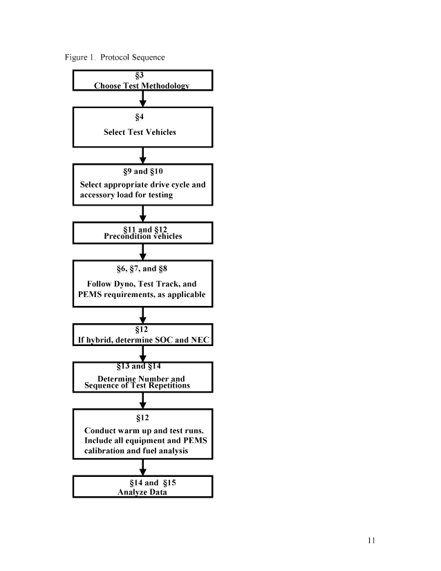
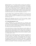
Figure xx shows the steps in the overall conduct of the testing, for whichever path has
been chosen.
The following overview is designed to help the user determine which test method is more
appropriate for their needs.
image:
• Intermodal drayage truck
The heavy duty vehicle categories listed in this test protocol overlap but don't fall
perfectly within existing intended service categories for heavy duty diesel engines, as
defined in the federal emissions certification program. According to 40 CFR §86.090-2,
the intended service category for a heavy duty engine is the primary service application
group for which a heavy duty diesel engine is designed and marketed, as determined by
the manufacturer. The determination is based on factors such as vehicle GVWR, vehicle
usage and operating patterns, vehicle design, engine horsepower, and engine design and
operating characteristics.
3. Overview of Test Methods
The fuel consumption of the test vehicle is measured by operating the vehicle on either a
test track or on a chassis dynamometer over a specified drive cycle and measuring the
fuel consumption. Fuel consumption can be calculated on the basis of a mass balance of
carbon-bearing emission gases (CC>2, CO, CH/t, other hydrocarbons) as described in 40
CFR Part 86 and SAE test method J1094a4 or on the basis of a gravimetric fuel
measurement system using portable fuel tanks as described in SAE test method J1321, in
which the mass of fuel consumed is converted to volume using measurements of fuel
density.
Track tests can be conducted using either the gravimetric method or the carbon mass-
balance method using a portable emissions monitoring system, or PEMS.
Chassis dynamometer tests are conducted using the carbon-balance method and
laboratory gas analysis instrumentation (preferable) or the gravimetric method.
This test procedure does not address the comparability of track testing to chassis
dynamometer testing. More data is needed to develop robust correlation factors.
Preliminary testing indicates a dynamometer-to-track difference in the range of 4% to
10%. This difference may be explained by tire/surface interactions and test-to-test
variability. However, both track and chassis dynamometer tests demonstrated
directionally consistent and statistically equivalent differences to changes in drive cycle
for various vehicles.5 EPA encourages comments regarding possible methods for
correlating results of track tests and dynamometer tests. Comments received to date
suggest a preference for laboratory dynamometer testing, but EPA would like to retain a
standardized track test method in this document, if only to provide a means to relate the
results of dynamometer testing to more realistic on-road performance.
Figure xx shows the steps in the overall conduct of the testing, for whichever path has
been chosen.
The following overview is designed to help the user determine which test method is more
appropriate for their needs.
image:
 3.1 Track Test
A track test is a vehicle test conducted on an outside test track. Test tracks may be found
at vehicle proving grounds or other facilities specifically designed for vehicle or tire
performance testing. Although any type of heavy duty vehicle can be tested on a test
track, this option may be more suited to typical over-the-road heavy duty vehicles, like
combination tractor-trailers.6
Because the test involves the vehicle being operated on a road surface in a manner similar
to that of on-road driving, rolling resistance, aerodynamic drag, and inertial road load
power requirements are incorporated in the test measurement, and do not have to be
determined beforehand with a coastdown test and calculations. Although the result of a
track test reflects real-world vehicle performance better than a chassis dynamometer test,
by directly evaluating the impacts of road effects such as aerodynamic drag of tractors
and trailers and rolling resistance effects of tires, variability of ambient conditions may
result in greater variability of test results.7 This protocol includes specification of
ambient conditions as well as specifications for measurement of fuel consumption.
Additionally, a coastdown test should be performed to document the road load force the
vehicle experiences during the track test. See section 13.4 for details.
10
image:
3.1 Track Test
A track test is a vehicle test conducted on an outside test track. Test tracks may be found
at vehicle proving grounds or other facilities specifically designed for vehicle or tire
performance testing. Although any type of heavy duty vehicle can be tested on a test
track, this option may be more suited to typical over-the-road heavy duty vehicles, like
combination tractor-trailers.6
Because the test involves the vehicle being operated on a road surface in a manner similar
to that of on-road driving, rolling resistance, aerodynamic drag, and inertial road load
power requirements are incorporated in the test measurement, and do not have to be
determined beforehand with a coastdown test and calculations. Although the result of a
track test reflects real-world vehicle performance better than a chassis dynamometer test,
by directly evaluating the impacts of road effects such as aerodynamic drag of tractors
and trailers and rolling resistance effects of tires, variability of ambient conditions may
result in greater variability of test results.7 This protocol includes specification of
ambient conditions as well as specifications for measurement of fuel consumption.
Additionally, a coastdown test should be performed to document the road load force the
vehicle experiences during the track test. See section 13.4 for details.
10
image:
 Figure 1. Protocol Sequence
§3
Choose Test Methodology
I
§4
Select Test Vehicles
§9 and §10
Select appropriate drive cycle and
accessory load for testing
§11 and §12
Precondition vehicles
I
§6, §7, and §8
Follow Dyno, Test Track, and
PEMS requirements, as applicable
§12
If hybrid, determine SOC and NEC
I
§13 and §14
Determine Number and
Sequence of Test Repetitions
§12
Conduct warm up and test runs.
Include all equipment and PEMS
calibration and fuel analysis
I
§14 and §15
Analyze Data
11
image:
Figure 1. Protocol Sequence
§3
Choose Test Methodology
I
§4
Select Test Vehicles
§9 and §10
Select appropriate drive cycle and
accessory load for testing
§11 and §12
Precondition vehicles
I
§6, §7, and §8
Follow Dyno, Test Track, and
PEMS requirements, as applicable
§12
If hybrid, determine SOC and NEC
I
§13 and §14
Determine Number and
Sequence of Test Repetitions
§12
Conduct warm up and test runs.
Include all equipment and PEMS
calibration and fuel analysis
I
§14 and §15
Analyze Data
11
image:
 Detailed methodology for the gravimetric method of measuring fuel consumption is
described in §§5.7.1 and 5.7.3 of the joint TMC/SAE Fuel Consumption Test Procedure -
Type II, Surface Vehicle Recommended Practice J1321 (SAE J1321). Fuel consumption
is measured by weighing the fuel consumed using a portable fuel tank. In this method, a
portable fuel tank is weighed empty, filled with fuel, weighed again, and then mounted
on the test vehicle. The test vehicle's fuel line is connected to the portable tank the
moment the test begins, and disconnected at the conclusion of the drive cycle, after which
the portable tank is removed and reweighed. The fuel consumed during the test is
calculated using the density of the fuel and the difference in the weight of the portable
fuel tank before and after the test, to yield the volume (gallons) of fuel used.
The carbon balance method of measuring fuel consumption on the basis of SAE test
method 1094a (and in accordance with CFR 40 Part 86) uses an onboard portable
emissions monitoring system (PEMS) to measure the mass of carbon emitted in the
exhaust, as well as the exhaust flow. The PEMS records this information via an onboard
data acquisitions system.
Details for PEMS requirements can be found in 40 CFR Part 1065, Subpart J. Because
PEMS became commercially available only recently, the portable tank gravimetric
method has been more extensively used for track tests in the past.
3.2 Chassis Dynamometer Test
A chassis dynamometer test is a test conducted indoors on a hydrokinetic chassis
dynamometer. The chassis dynamometer option in this test procedure incorporates many
of the methods and requirements established in the federal light duty vehicle and 'light'
heavy duty vehicle emissions certification chassis test procedure. Although most heavy
duty vehicles can be tested on a chassis dynamometer, this option may be more suitable
for single unit truck and truck body heavy duty vehicles.8
Chassis dynamometers may be found at vehicle test laboratories; typically, facilities used
for emissions and vehicle fuel efficiency testing. Because the test is conducted on a
chassis dynamometer, rolling resistance, aerodynamic drag and inertial road load power
requirements must be determined ahead of time, with coastdown tests and calculations to
determine the proper horsepower absorption setting for the chassis dynamometer. Details
for conducting coastdown tests are found in the section of this test procedure covering the
chassis dynamometer test method.
When using the chassis dynamometer option in this test procedure, fuel consumption can
be measured using the carbon balance method, in which fuel consumption can be
calculated on the basis of a mass balance of carbon-bearing emission gases (CO2, CO,
CH4, other hydrocarbons) as described in SAE test method J1094a. In this method,
vehicle emissions are collected and analyzed using laboratory gas analyzer equipment.
The laboratory equipment measures and records the concentration of carbon-based
compounds emitted in the exhaust as well as the exhaust flow. The concentrations and
densities of the carbon-based compounds, and exhaust flow values, are used to calculate
the mass of fuel consumed. The volume of fuel consumed is determined by the mass of
12
image:
Detailed methodology for the gravimetric method of measuring fuel consumption is
described in §§5.7.1 and 5.7.3 of the joint TMC/SAE Fuel Consumption Test Procedure -
Type II, Surface Vehicle Recommended Practice J1321 (SAE J1321). Fuel consumption
is measured by weighing the fuel consumed using a portable fuel tank. In this method, a
portable fuel tank is weighed empty, filled with fuel, weighed again, and then mounted
on the test vehicle. The test vehicle's fuel line is connected to the portable tank the
moment the test begins, and disconnected at the conclusion of the drive cycle, after which
the portable tank is removed and reweighed. The fuel consumed during the test is
calculated using the density of the fuel and the difference in the weight of the portable
fuel tank before and after the test, to yield the volume (gallons) of fuel used.
The carbon balance method of measuring fuel consumption on the basis of SAE test
method 1094a (and in accordance with CFR 40 Part 86) uses an onboard portable
emissions monitoring system (PEMS) to measure the mass of carbon emitted in the
exhaust, as well as the exhaust flow. The PEMS records this information via an onboard
data acquisitions system.
Details for PEMS requirements can be found in 40 CFR Part 1065, Subpart J. Because
PEMS became commercially available only recently, the portable tank gravimetric
method has been more extensively used for track tests in the past.
3.2 Chassis Dynamometer Test
A chassis dynamometer test is a test conducted indoors on a hydrokinetic chassis
dynamometer. The chassis dynamometer option in this test procedure incorporates many
of the methods and requirements established in the federal light duty vehicle and 'light'
heavy duty vehicle emissions certification chassis test procedure. Although most heavy
duty vehicles can be tested on a chassis dynamometer, this option may be more suitable
for single unit truck and truck body heavy duty vehicles.8
Chassis dynamometers may be found at vehicle test laboratories; typically, facilities used
for emissions and vehicle fuel efficiency testing. Because the test is conducted on a
chassis dynamometer, rolling resistance, aerodynamic drag and inertial road load power
requirements must be determined ahead of time, with coastdown tests and calculations to
determine the proper horsepower absorption setting for the chassis dynamometer. Details
for conducting coastdown tests are found in the section of this test procedure covering the
chassis dynamometer test method.
When using the chassis dynamometer option in this test procedure, fuel consumption can
be measured using the carbon balance method, in which fuel consumption can be
calculated on the basis of a mass balance of carbon-bearing emission gases (CO2, CO,
CH4, other hydrocarbons) as described in SAE test method J1094a. In this method,
vehicle emissions are collected and analyzed using laboratory gas analyzer equipment.
The laboratory equipment measures and records the concentration of carbon-based
compounds emitted in the exhaust as well as the exhaust flow. The concentrations and
densities of the carbon-based compounds, and exhaust flow values, are used to calculate
the mass of fuel consumed. The volume of fuel consumed is determined by the mass of
12
image:
 fuel consumed and the density of the fuel. This method of measuring heavy duty vehicle
fuel consumption on a chassis dynamometer is substantially similar to the method used to
measure fuel efficiency for passenger vehicles.
Detailed procedures for conducting chassis dynamometer testing are provided in the
optional complete vehicle federal emissions certification method for light heavy duty
vehicles, applicable to heavy duty vehicles with a GVWR of 8,500 to 14,000 pounds.
The chassis emissions test procedure is detailed in 40 CFR §86.1816-05, 40 CFR
§86.1816-08, and 40 CFR §86.1863-07. For heavy duty vehicles up to 14,000 pounds,
the heavy duty fuel efficiency test procedure described in this document follows the
provisions outlined in 40 CFR part §86.1863. The provisions outlined in 40 CFR part
§86.1863 dealing with evaporative emission testing, on-board diagnostic (OBD)
requirements, smoke emission requirements, and requirements for measuring criteria
pollutants do not apply. Although, at the user's discretion, these additional components
can be included in a fuel efficiency test.
For test vehicles exceeding 14,000 Ibs GVWR, there is no pre-existing federal chassis
dynamometer test procedure. For these vehicles, the test procedure described in this
document uses many of the precedents established in 40 CFR Part 86, with the exception
of the requirement for a higher capacity chassis dynamometer. This procedure provides
new chassis dynamometer requirements to accommodate larger vehicle testing. In all
cases, the following guidelines should be followed:
• Dynamometer coefficients that simulate road-load forces shall be determined as
specified in SAE J2263 and J2264.
• Dynamometer power absorption and inertia simulation shall be set as specified in
40 CFR Part 86-1229-85.
• Test instrumentation equipment (including where appropriate, exhaust emissions
sampling and analytical systems) as referenced in 40 CFR Part 86.1301-90 to 40
CFR 86.1326-90 and/or 40 CFR Part 1065 shall be calibrated in a manner that is
NIST-traceable.
4. Vehicle Selection
Vehicles shall be representative of production fleet vehicles. The test vehicle must be
appropriate for its service category. It should have the same vehicle "package," that is,
body style, equipment, number of axles, gross vehicle weight rating (GVWR), and
accessories, that enable the complete vehicle to accomplish the type of service
(performance, utility, durability, etc.) for its intended application. Equipment
specifications that can affect fuel efficiency (engine size and type, tire size and type,
transmission size and type, brakes, gear shift points, rear axle ratio, air suspension,
lubricant type, idle RPM, ignition timing, wheel alignment, etc.) must be representative
of how that vehicle is driven on the road, and used to perform work.
13
image:
fuel consumed and the density of the fuel. This method of measuring heavy duty vehicle
fuel consumption on a chassis dynamometer is substantially similar to the method used to
measure fuel efficiency for passenger vehicles.
Detailed procedures for conducting chassis dynamometer testing are provided in the
optional complete vehicle federal emissions certification method for light heavy duty
vehicles, applicable to heavy duty vehicles with a GVWR of 8,500 to 14,000 pounds.
The chassis emissions test procedure is detailed in 40 CFR §86.1816-05, 40 CFR
§86.1816-08, and 40 CFR §86.1863-07. For heavy duty vehicles up to 14,000 pounds,
the heavy duty fuel efficiency test procedure described in this document follows the
provisions outlined in 40 CFR part §86.1863. The provisions outlined in 40 CFR part
§86.1863 dealing with evaporative emission testing, on-board diagnostic (OBD)
requirements, smoke emission requirements, and requirements for measuring criteria
pollutants do not apply. Although, at the user's discretion, these additional components
can be included in a fuel efficiency test.
For test vehicles exceeding 14,000 Ibs GVWR, there is no pre-existing federal chassis
dynamometer test procedure. For these vehicles, the test procedure described in this
document uses many of the precedents established in 40 CFR Part 86, with the exception
of the requirement for a higher capacity chassis dynamometer. This procedure provides
new chassis dynamometer requirements to accommodate larger vehicle testing. In all
cases, the following guidelines should be followed:
• Dynamometer coefficients that simulate road-load forces shall be determined as
specified in SAE J2263 and J2264.
• Dynamometer power absorption and inertia simulation shall be set as specified in
40 CFR Part 86-1229-85.
• Test instrumentation equipment (including where appropriate, exhaust emissions
sampling and analytical systems) as referenced in 40 CFR Part 86.1301-90 to 40
CFR 86.1326-90 and/or 40 CFR Part 1065 shall be calibrated in a manner that is
NIST-traceable.
4. Vehicle Selection
Vehicles shall be representative of production fleet vehicles. The test vehicle must be
appropriate for its service category. It should have the same vehicle "package," that is,
body style, equipment, number of axles, gross vehicle weight rating (GVWR), and
accessories, that enable the complete vehicle to accomplish the type of service
(performance, utility, durability, etc.) for its intended application. Equipment
specifications that can affect fuel efficiency (engine size and type, tire size and type,
transmission size and type, brakes, gear shift points, rear axle ratio, air suspension,
lubricant type, idle RPM, ignition timing, wheel alignment, etc.) must be representative
of how that vehicle is driven on the road, and used to perform work.
13
image:
 Test vehicles need not be new, but they must be in good mechanical order and operating
condition, with no obvious mechanical or physical defects that might affect fuel
efficiency. If new, the vehicle should be broken in per the manufacturer's recommended
procedures, at a minimum. Refer to the requirements for mechanical and operating
condition described in SAE J1321 §8.7.9 All components and equipment shall be
calibrated and maintained to within manufacturer-recommended specifications. The
exception is any component that has been deliberately modified as part of the test truck
design.
To ensure proper vehicle operability, it is recommended that the engine and emission
control equipment meet the emissions performance certification for the given model year.
If a heavy duty vehicle is typically used in combination with a trailer or truck body, the
test will produce a more comprehensive fuel efficiency result if the vehicle is tested in
combination with a trailer or truck body. In certain instances, testing with a trailer or
truck body is necessary; for example, in track testing, to provide the proper payload
required, or when testing the impact of aerodynamic design elements for use in a tractor-
trailer combination vehicle.
If a heavy duty vehicle is tested with a truck body or trailer, then the truck body or trailer
shall be appropriate for that vehicle's intended service. It is recommended to use a trailer
or truck body that is representative in design, function, weight, and dimension, of the type
of trailer or truck body typical for that application. An exception is if modifications to a
trailer or truck body are part of the vehicle design being tested. Whenever a trailer or
truck body is tested with a heavy duty vehicle, the same trailer or truck body must remain
paired with the test vehicle throughout the duration of the testing program.
Unless otherwise indicated, the following trailer specifications are recommended for a
typical highway line haul tractor-trailer combination:
• dry van box trailer
• 2 trailer axles
• 53' long, 102" wide, 13'6" high
• minimized trailer gap (maximum of 45" depending upon kingpin setting)
• 11,000 to 14,000 pounds
Truck body specifications shall be appropriate to each intended application.
When selecting a test vehicle, if the purpose is to compare its performance to other
vehicles in that application, then the vehicles selected shall be closely matched in class,
model year, body style, equipment, fuel type, accessories, mileage, and condition, with
the exception of any vehicle design options being tested.10
5. Test Fuel
For vehicles with compression-ignition engines certified on diesel fuel, the test fuel shall
be number 2 distillate ultra-low sulfur diesel fuel (ULSD). The test fuel will meet fuel
14
image:
Test vehicles need not be new, but they must be in good mechanical order and operating
condition, with no obvious mechanical or physical defects that might affect fuel
efficiency. If new, the vehicle should be broken in per the manufacturer's recommended
procedures, at a minimum. Refer to the requirements for mechanical and operating
condition described in SAE J1321 §8.7.9 All components and equipment shall be
calibrated and maintained to within manufacturer-recommended specifications. The
exception is any component that has been deliberately modified as part of the test truck
design.
To ensure proper vehicle operability, it is recommended that the engine and emission
control equipment meet the emissions performance certification for the given model year.
If a heavy duty vehicle is typically used in combination with a trailer or truck body, the
test will produce a more comprehensive fuel efficiency result if the vehicle is tested in
combination with a trailer or truck body. In certain instances, testing with a trailer or
truck body is necessary; for example, in track testing, to provide the proper payload
required, or when testing the impact of aerodynamic design elements for use in a tractor-
trailer combination vehicle.
If a heavy duty vehicle is tested with a truck body or trailer, then the truck body or trailer
shall be appropriate for that vehicle's intended service. It is recommended to use a trailer
or truck body that is representative in design, function, weight, and dimension, of the type
of trailer or truck body typical for that application. An exception is if modifications to a
trailer or truck body are part of the vehicle design being tested. Whenever a trailer or
truck body is tested with a heavy duty vehicle, the same trailer or truck body must remain
paired with the test vehicle throughout the duration of the testing program.
Unless otherwise indicated, the following trailer specifications are recommended for a
typical highway line haul tractor-trailer combination:
• dry van box trailer
• 2 trailer axles
• 53' long, 102" wide, 13'6" high
• minimized trailer gap (maximum of 45" depending upon kingpin setting)
• 11,000 to 14,000 pounds
Truck body specifications shall be appropriate to each intended application.
When selecting a test vehicle, if the purpose is to compare its performance to other
vehicles in that application, then the vehicles selected shall be closely matched in class,
model year, body style, equipment, fuel type, accessories, mileage, and condition, with
the exception of any vehicle design options being tested.10
5. Test Fuel
For vehicles with compression-ignition engines certified on diesel fuel, the test fuel shall
be number 2 distillate ultra-low sulfur diesel fuel (ULSD). The test fuel will meet fuel
14
image:
 specifications outlined in 40 CFR §80.520 for ULSD #2D distillate. The exception is if
fuel type is a design option being tested.
Specific fuel parameters include:
• Sulfur content. 15 parts per million (ppm) maximum
• Cetane index and aromatic content. Minimum cetane index of 40 or maximum
aromatic content of 35 volume percent.
• Flash/Fire point. 52° C minimum
• Water/Sediment. 0.05% volume maximum
• Particulate Contaminant. 10 mg/L maximum
• Viscosity KIN/CS at 40°C. 1.9 to 4.1
For vehicles with any Otto-cycle engine certified on gasoline, natural gas, propane, or
other fuels, the test fuel shall meet the fuel specifications outlined in 40 CFR §86.1313-
94, sections c through f
A supply of test fuel sufficient to complete the test must be procured and fuel parameters
including fuel density analyzed prior to the start of the test. If fuel consumption is to be
measured by the gravimetric method, the following additional test shall be made:
• ASTM Test Method D-1298, Standard Test Method for Density, Relative Density
(Specific Gravity), or API Gravity of Crude Petroleum and Liquid Petroleum
Products by Hydrometer.
The test fuel must be sequestered once it is procured and analyzed. If it is necessary to
add additional fuel to the test fuel supply during the course of the test, another fuel
analysis must be conducted to ensure the test fuel still meets the required fuel parameters.
For each test segment, a record must be kept of the fuel parameters of the test fuel,
including density.
6. Test Track Specifications and Requirements
If the option for on-road testing is chosen, the testing shall be conducted on a test track,
not on a public highway, to provide greater control of test conditions. This section
describes the general specifications and conditions for the test track.
6.1 Track Specifications
Setting specifications for the test track can minimize the effect of a track's physical
attributes on vehicle performance. The following are specification requirements for a test
track that will give good, repeatable results, while still allowing for a reasonable number
of track facilities to be used to conduct this test:
• Shape. Oval (recommended), figure eight, or serpentine to minimize the effects
of yaw angle wind effects and lateral forces. Circular tracks are not permitted.
• Neutral steering speed. The radii of the curves in conjunction with the banking
grade (superelevation) shall be selected to permit a minimum of 40 mph around
the curves. This can require a superelevation of 2% for curves with a 10,000 foot
radius or more. For curves with a radius of less than 10,000 feet, the super
elevation must be consistent with applicable state and federal DOT roadway
15
image:
specifications outlined in 40 CFR §80.520 for ULSD #2D distillate. The exception is if
fuel type is a design option being tested.
Specific fuel parameters include:
• Sulfur content. 15 parts per million (ppm) maximum
• Cetane index and aromatic content. Minimum cetane index of 40 or maximum
aromatic content of 35 volume percent.
• Flash/Fire point. 52° C minimum
• Water/Sediment. 0.05% volume maximum
• Particulate Contaminant. 10 mg/L maximum
• Viscosity KIN/CS at 40°C. 1.9 to 4.1
For vehicles with any Otto-cycle engine certified on gasoline, natural gas, propane, or
other fuels, the test fuel shall meet the fuel specifications outlined in 40 CFR §86.1313-
94, sections c through f
A supply of test fuel sufficient to complete the test must be procured and fuel parameters
including fuel density analyzed prior to the start of the test. If fuel consumption is to be
measured by the gravimetric method, the following additional test shall be made:
• ASTM Test Method D-1298, Standard Test Method for Density, Relative Density
(Specific Gravity), or API Gravity of Crude Petroleum and Liquid Petroleum
Products by Hydrometer.
The test fuel must be sequestered once it is procured and analyzed. If it is necessary to
add additional fuel to the test fuel supply during the course of the test, another fuel
analysis must be conducted to ensure the test fuel still meets the required fuel parameters.
For each test segment, a record must be kept of the fuel parameters of the test fuel,
including density.
6. Test Track Specifications and Requirements
If the option for on-road testing is chosen, the testing shall be conducted on a test track,
not on a public highway, to provide greater control of test conditions. This section
describes the general specifications and conditions for the test track.
6.1 Track Specifications
Setting specifications for the test track can minimize the effect of a track's physical
attributes on vehicle performance. The following are specification requirements for a test
track that will give good, repeatable results, while still allowing for a reasonable number
of track facilities to be used to conduct this test:
• Shape. Oval (recommended), figure eight, or serpentine to minimize the effects
of yaw angle wind effects and lateral forces. Circular tracks are not permitted.
• Neutral steering speed. The radii of the curves in conjunction with the banking
grade (superelevation) shall be selected to permit a minimum of 40 mph around
the curves. This can require a superelevation of 2% for curves with a 10,000 foot
radius or more. For curves with a radius of less than 10,000 feet, the super
elevation must be consistent with applicable state and federal DOT roadway
15
image:
 requirements. A minimum neutral steering speed is needed to prevent the test
vehicle from losing forward motion to lateral forces when negotiating a curve
"hands off."
• Length. A minimum of 1.5 miles, with 5 miles or more recommended. A track
of this length minimizes excessive curve radii and prevents the test vehicle from
losing forward motion when negotiating curves.
• Grade. The maximum grade change shall not exceed 2% longitudinally, to
prevent the test vehicle from excessive changes in forward motion due to grade.
• Surface. The surface shall be concrete or asphalt, to minimize energy absorption
effects of uneven or rough pavement. It is recommended that the friction and
surface characteristics comply with federal and state DOT specifications
regarding road condition.
• Altitude. The track shall be at an elevation no higher than 4,000 feet above sea
level, to minimize changes to air density that may alter the vehicle's forward
motion, and to prevent unintended changes in engine and subsystem operation.
• Maintenance. The test track shall be well-maintained, inspected at least once a
year, and resurfaced as needed to maintain surface integrity and consistency.
6.2 Track Requirements
The track shall have the capacity to measure and record test conditions, in order to ensure
that a test is conducted in accordance with the provisions of this test procedure. The
following are the minimum requirements needed to conduct a track test:
• Weather Monitoring. The track shall be equipped with the capacity to monitor
ambient conditions (wind direction and velocity, temperature, humidity,
barometric pressure) during each test. It is recommended that the weather sensing
equipment is located on the test track, or at a weather station within 50 miles of
the test track. Options for on-site weather monitoring equipment include: an
anemometer or a marine-type hand held wind indicator to monitor wind direction
and velocity11; a thermometer to measure temperature; a barometer to measure
barometric pressure; and a hygrometer to measure humidity. The positioning,
etc., of ambient condition sensors shall be consistent with provisions outlined in
the Federal Standard for Siting Meteorological Sensors at Airports, FCM-S4-
1987. The track shall have the capacity to record this weather information, as part
of the test record.
• Truck Weight Scales. The track shall be equipped with properly calibrated truck
weight scales (or located within 50 miles of the test track) that conform to the
most current provisions established by the National Institute of Standards and
Technology (NIST). As of the writing of this test procedure, these provisions are
those published in the NIST Handbook 44 - 2007 Edition, Specifications,
Tolerances, and Other Technical Requirements for Weighing and Measuring
Devices. The truck scales must be calibrated annually at a minimum. It is
recommended that the truck scales have a National Type Evaluation Program
(NTEP) Certificate of Conformance.
• Portable Scales. If the portable fuel tank gravimetric method is used, the track
shall be equipped with properly calibrated portable scales that conform to
provisions established in SAE J1321 §5.7.1 and §8.4. Scales should have a
16
image:
requirements. A minimum neutral steering speed is needed to prevent the test
vehicle from losing forward motion to lateral forces when negotiating a curve
"hands off."
• Length. A minimum of 1.5 miles, with 5 miles or more recommended. A track
of this length minimizes excessive curve radii and prevents the test vehicle from
losing forward motion when negotiating curves.
• Grade. The maximum grade change shall not exceed 2% longitudinally, to
prevent the test vehicle from excessive changes in forward motion due to grade.
• Surface. The surface shall be concrete or asphalt, to minimize energy absorption
effects of uneven or rough pavement. It is recommended that the friction and
surface characteristics comply with federal and state DOT specifications
regarding road condition.
• Altitude. The track shall be at an elevation no higher than 4,000 feet above sea
level, to minimize changes to air density that may alter the vehicle's forward
motion, and to prevent unintended changes in engine and subsystem operation.
• Maintenance. The test track shall be well-maintained, inspected at least once a
year, and resurfaced as needed to maintain surface integrity and consistency.
6.2 Track Requirements
The track shall have the capacity to measure and record test conditions, in order to ensure
that a test is conducted in accordance with the provisions of this test procedure. The
following are the minimum requirements needed to conduct a track test:
• Weather Monitoring. The track shall be equipped with the capacity to monitor
ambient conditions (wind direction and velocity, temperature, humidity,
barometric pressure) during each test. It is recommended that the weather sensing
equipment is located on the test track, or at a weather station within 50 miles of
the test track. Options for on-site weather monitoring equipment include: an
anemometer or a marine-type hand held wind indicator to monitor wind direction
and velocity11; a thermometer to measure temperature; a barometer to measure
barometric pressure; and a hygrometer to measure humidity. The positioning,
etc., of ambient condition sensors shall be consistent with provisions outlined in
the Federal Standard for Siting Meteorological Sensors at Airports, FCM-S4-
1987. The track shall have the capacity to record this weather information, as part
of the test record.
• Truck Weight Scales. The track shall be equipped with properly calibrated truck
weight scales (or located within 50 miles of the test track) that conform to the
most current provisions established by the National Institute of Standards and
Technology (NIST). As of the writing of this test procedure, these provisions are
those published in the NIST Handbook 44 - 2007 Edition, Specifications,
Tolerances, and Other Technical Requirements for Weighing and Measuring
Devices. The truck scales must be calibrated annually at a minimum. It is
recommended that the truck scales have a National Type Evaluation Program
(NTEP) Certificate of Conformance.
• Portable Scales. If the portable fuel tank gravimetric method is used, the track
shall be equipped with properly calibrated portable scales that conform to
provisions established in SAE J1321 §5.7.1 and §8.4. Scales should have a
16
image:
 resolution of 0.1% of the expected fuel mass consumed, or better. Portable scales
must be calibrated annually at a minimum. Portable scale function should be
verified with a check weight prior to the weighing operation.
• Portable Emissions Monitoring System (PEMS). If the PEMS carbon balance
method is used, the operators conducting the test shall have the capability to
properly use and maintain a portable emissions monitoring system (PEMS), as
recommended by the PEMS manufacturer, and as required by 40 CFRPart 1065.
This includes providing all equipment and materials needed to properly use and
maintain the PEMS. In addition to the electronic flow meter, gas analyzer, heated
lines, etc., integral to the PEMS, ancillary equipment and materials include zero,
calibration and span gases; gas pressure and flow regulators and gauges; data
loggers; all connectors and hoses. The PEMS and all PEMS-related equipment
and supplies shall be calibrated and maintained as recommended by the PEMS
manufacturer, and as required by 40 CFR Part 1065 Subpart D. Additional
requirements governing the use of PEMS are detailed in Section §8 of this test
procedure.
• Speed and Distance Equipment. The test vehicle must be equipped with a
means to measure speed and distance. A global position sensor (GPS) is
recommended, as an adjunct to vehicle electronic control module (ECM) data
and/or speedometer and odometer readings. The accuracy of the odometer and
speedometer must be verified and corrections made if necessary. This can be
accomplished using a stop watch and the track lane length at the specified speed.
Reference SAE J1321 §8.12. The track must be equipped with markers that can
be positioned to match target speed and distance parameters of the selected drive
cycle, including gear shift and braking points. Using a global position sensor
(GPS) is recommended, as an adjunct to ECM data and/or speedometer and
odometer readings.
6.3 Track Environmental Requirements
A track test is not intended to replicate the tightly-controlled environment of a laboratory
test, since a key attribute of track testing is the ability to more closely simulate in-use
operation. Nor would such tight controls be feasible on a track test. However, setting
appropriate parameters for ambient conditions can improve the repeatability and
reproducibility of track test results. The following limits allow for reasonable variation in
the ambient conditions under which track tests can occur:
• Temperature. Testing shall occur when the ambient temperature is between
68°F to 86°F (20°C to 30°C). If the ambient temperature changes by more than
20°F over the course of the testing, all testing will be repeated. The temperature
in the fuel tank cannot exceed 160°F. Reference SAE J1321 §5.7.3. 12 When
using the PEMS method, a test run shall be invalidated if an ambient temperature
warning on the PEMS occurs during the test.
• Humidity. Testing can be conducted at any humidity level; however, an optimal
range is between 35% and 75% relative humidity; 40% is ideal.
• Wind. Testing shall occur when wind speeds are at 12 mph or less, with wind
gusts no greater than 15 mph.
17
image:
resolution of 0.1% of the expected fuel mass consumed, or better. Portable scales
must be calibrated annually at a minimum. Portable scale function should be
verified with a check weight prior to the weighing operation.
• Portable Emissions Monitoring System (PEMS). If the PEMS carbon balance
method is used, the operators conducting the test shall have the capability to
properly use and maintain a portable emissions monitoring system (PEMS), as
recommended by the PEMS manufacturer, and as required by 40 CFRPart 1065.
This includes providing all equipment and materials needed to properly use and
maintain the PEMS. In addition to the electronic flow meter, gas analyzer, heated
lines, etc., integral to the PEMS, ancillary equipment and materials include zero,
calibration and span gases; gas pressure and flow regulators and gauges; data
loggers; all connectors and hoses. The PEMS and all PEMS-related equipment
and supplies shall be calibrated and maintained as recommended by the PEMS
manufacturer, and as required by 40 CFR Part 1065 Subpart D. Additional
requirements governing the use of PEMS are detailed in Section §8 of this test
procedure.
• Speed and Distance Equipment. The test vehicle must be equipped with a
means to measure speed and distance. A global position sensor (GPS) is
recommended, as an adjunct to vehicle electronic control module (ECM) data
and/or speedometer and odometer readings. The accuracy of the odometer and
speedometer must be verified and corrections made if necessary. This can be
accomplished using a stop watch and the track lane length at the specified speed.
Reference SAE J1321 §8.12. The track must be equipped with markers that can
be positioned to match target speed and distance parameters of the selected drive
cycle, including gear shift and braking points. Using a global position sensor
(GPS) is recommended, as an adjunct to ECM data and/or speedometer and
odometer readings.
6.3 Track Environmental Requirements
A track test is not intended to replicate the tightly-controlled environment of a laboratory
test, since a key attribute of track testing is the ability to more closely simulate in-use
operation. Nor would such tight controls be feasible on a track test. However, setting
appropriate parameters for ambient conditions can improve the repeatability and
reproducibility of track test results. The following limits allow for reasonable variation in
the ambient conditions under which track tests can occur:
• Temperature. Testing shall occur when the ambient temperature is between
68°F to 86°F (20°C to 30°C). If the ambient temperature changes by more than
20°F over the course of the testing, all testing will be repeated. The temperature
in the fuel tank cannot exceed 160°F. Reference SAE J1321 §5.7.3. 12 When
using the PEMS method, a test run shall be invalidated if an ambient temperature
warning on the PEMS occurs during the test.
• Humidity. Testing can be conducted at any humidity level; however, an optimal
range is between 35% and 75% relative humidity; 40% is ideal.
• Wind. Testing shall occur when wind speeds are at 12 mph or less, with wind
gusts no greater than 15 mph.
17
image:
 • Precipitation. Testing shall occur during conditions of no visible precipitation
and no moisture on the test track surface, which would contact the tires. No
visible precipitation is defined as precipitation of 0.1 mm (per hour??) or less.
Testing shall occur only when the track is dry, and there is no precipitation or fog.
Information about environmental conditions during a test shall be available during or
after the test, to determine the test's validity, and records shall be kept as part of the test
documentation.
7. Chassis Dynamometer Specifications and Requirements
Detailed procedures to conduct chassis dynamometer testing are provided in 40 CFR Part
86, SubpartB. If one opts to test to §86.1863, SubpartB can be used. If a test vehicle
exceeds 14,000 pounds GVWR, then a higher capacity chassis dynamometer may need to
be used. Recommended specifications for a higher capacity chassis dynamometer are
listed below.
7.1 Chassis Dynamometer Specifications
The chassis dynamometer specifications for testing heavy duty vehicles with a GVWR of
less than 14,000 pounds but more than 8,500 pounds shall be similar to the requirements
found in 40 CFR Part 86, Subpart B for the testing of light duty cars and trucks. Section
§86.108-00 of the CFR includes provisions for both small twin roll (8.65-inch diameter)
and large, single-roll (48-inch) dynamometers. A large, single-roll electric dynamometer
is preferable, unless a vehicle is more suited for testing on a twin roll dynamometer (e.g.,
if disengaging one of the axles on a twin-screw drive axle would create a safety or
operational problem). If a twin roll hydrokinetic dynamometer is used, the results must
be correlated to that of a single roll electric chassis dynamometer.13 For vehicles with a
GVWR greater than 14,000 pounds, the heavy duty chassis dynamometer used to test the
vehicle shall have a sufficient capacity to test the vehicle at its rated test weight for the
application.
If the tested vehicle exceeds 14,000 pounds GVWR, the testing organization shall refer to
the following recommended specifications.
HEAVY DUTY VEHICLE CHASSIS DYNAMOMETER SPECIFICATIONS
GENERAL FACILITY INFORMATION
GVWR capability > 14,000 Ibs
Rear Axle Weight Capability 5,000 to 44,000 Ibs
Speed Range 0 to 65 mph
Power absorption 0 to 500 hp
Power motoring 0 to 500 hp
Tractive Force 3000 Ibs-f
Roll Diameter 24 to 72 in
Lab Environment Temperature 68°F to 86°F
Range
Combustion air temperature No
18
image:
• Precipitation. Testing shall occur during conditions of no visible precipitation
and no moisture on the test track surface, which would contact the tires. No
visible precipitation is defined as precipitation of 0.1 mm (per hour??) or less.
Testing shall occur only when the track is dry, and there is no precipitation or fog.
Information about environmental conditions during a test shall be available during or
after the test, to determine the test's validity, and records shall be kept as part of the test
documentation.
7. Chassis Dynamometer Specifications and Requirements
Detailed procedures to conduct chassis dynamometer testing are provided in 40 CFR Part
86, SubpartB. If one opts to test to §86.1863, SubpartB can be used. If a test vehicle
exceeds 14,000 pounds GVWR, then a higher capacity chassis dynamometer may need to
be used. Recommended specifications for a higher capacity chassis dynamometer are
listed below.
7.1 Chassis Dynamometer Specifications
The chassis dynamometer specifications for testing heavy duty vehicles with a GVWR of
less than 14,000 pounds but more than 8,500 pounds shall be similar to the requirements
found in 40 CFR Part 86, Subpart B for the testing of light duty cars and trucks. Section
§86.108-00 of the CFR includes provisions for both small twin roll (8.65-inch diameter)
and large, single-roll (48-inch) dynamometers. A large, single-roll electric dynamometer
is preferable, unless a vehicle is more suited for testing on a twin roll dynamometer (e.g.,
if disengaging one of the axles on a twin-screw drive axle would create a safety or
operational problem). If a twin roll hydrokinetic dynamometer is used, the results must
be correlated to that of a single roll electric chassis dynamometer.13 For vehicles with a
GVWR greater than 14,000 pounds, the heavy duty chassis dynamometer used to test the
vehicle shall have a sufficient capacity to test the vehicle at its rated test weight for the
application.
If the tested vehicle exceeds 14,000 pounds GVWR, the testing organization shall refer to
the following recommended specifications.
HEAVY DUTY VEHICLE CHASSIS DYNAMOMETER SPECIFICATIONS
GENERAL FACILITY INFORMATION
GVWR capability > 14,000 Ibs
Rear Axle Weight Capability 5,000 to 44,000 Ibs
Speed Range 0 to 65 mph
Power absorption 0 to 500 hp
Power motoring 0 to 500 hp
Tractive Force 3000 Ibs-f
Roll Diameter 24 to 72 in
Lab Environment Temperature 68°F to 86°F
Range
Combustion air temperature No
18
image:
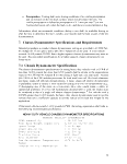 control? (y/n)
Combustion air humidity No
control? (y/n)
MOTOR AND POWER CONTROL
Motor Type
Manual or automated drive
cycle
Nominal power (standard)
Nominal power (maximum)
Drive Torque (standard)
Drive Torque
DC or AC motors (approx range
500 hp)
Automated
(maximum)
400 hp
500 hp
5000 Ib-ft
8000 Ib-ft
ACCELERATION MEASUREMENT
Acceleration, maximum 5 to 15 ft/sec2
Deceleration, maximum 5 to 15 ft/sec2
EMISSIONS CAPABILITY
Bag method, or continuous raw
Acceptable types
NOx
PM
HC
CO
C02
Fuel flow
Fuel type capability
smpl.
Not required
Not required
FID
NDIR or FTIR
NDIR or FTIR
Carbon balance
Diesel, CNG, gasoline,
propane
7.2 Chassis Dynamometer Requirements
A requirement for either type of chassis dynamometer (single or twin roll) is that it shall
permit the user to convert coastdown data for the test vehicle to the proper horsepower
absorption setting for the chassis dynamometer. A coastdown test must be conducted and
the results converted to dynamometer settings using published SAE procedures.14 15
Coastdown data shall be taken with the vehicle at full test weight to determine the proper
dynamometer settings. Additional details on how to conduct a vehicle coastdown test
and convert the results to the proper horsepower absorption setting in chassis
dynamometer tests is found in Section §12 of this document.
Either type of chassis dynamometer (single or twin roll) shall be equipped with a cooling
fan to provide cooling air flow to the vehicle during testing. Refer to 40 CFR Part
86.107-96 (d) for vehicle cooling fan requirements. A road-speed modulating fan shall
be used, rather than a fixed-speed cooling fan.
Refer to 40 CFR Part 86.108-79 and 86.108-00 for chassis dynamometer equipment
specifications. Refer to 40 CFR 86.118-00 and 40 CFR 86.118-78 and 40 CFR Part
86.116-90 through 86.116-94 for chassis dynamometer calibration requirements.
19
image:
control? (y/n)
Combustion air humidity No
control? (y/n)
MOTOR AND POWER CONTROL
Motor Type
Manual or automated drive
cycle
Nominal power (standard)
Nominal power (maximum)
Drive Torque (standard)
Drive Torque
DC or AC motors (approx range
500 hp)
Automated
(maximum)
400 hp
500 hp
5000 Ib-ft
8000 Ib-ft
ACCELERATION MEASUREMENT
Acceleration, maximum 5 to 15 ft/sec2
Deceleration, maximum 5 to 15 ft/sec2
EMISSIONS CAPABILITY
Bag method, or continuous raw
Acceptable types
NOx
PM
HC
CO
C02
Fuel flow
Fuel type capability
smpl.
Not required
Not required
FID
NDIR or FTIR
NDIR or FTIR
Carbon balance
Diesel, CNG, gasoline,
propane
7.2 Chassis Dynamometer Requirements
A requirement for either type of chassis dynamometer (single or twin roll) is that it shall
permit the user to convert coastdown data for the test vehicle to the proper horsepower
absorption setting for the chassis dynamometer. A coastdown test must be conducted and
the results converted to dynamometer settings using published SAE procedures.14 15
Coastdown data shall be taken with the vehicle at full test weight to determine the proper
dynamometer settings. Additional details on how to conduct a vehicle coastdown test
and convert the results to the proper horsepower absorption setting in chassis
dynamometer tests is found in Section §12 of this document.
Either type of chassis dynamometer (single or twin roll) shall be equipped with a cooling
fan to provide cooling air flow to the vehicle during testing. Refer to 40 CFR Part
86.107-96 (d) for vehicle cooling fan requirements. A road-speed modulating fan shall
be used, rather than a fixed-speed cooling fan.
Refer to 40 CFR Part 86.108-79 and 86.108-00 for chassis dynamometer equipment
specifications. Refer to 40 CFR 86.118-00 and 40 CFR 86.118-78 and 40 CFR Part
86.116-90 through 86.116-94 for chassis dynamometer calibration requirements.
19
image:
 Additional details covering the chassis dynamometer test procedure are found in Section
§12 of this document.
7.3 Chassis Dynamometer Environmental Requirements
Testing conditions are consistent with the requirements established in 40 CFR Part 86 for
federal vehicle emissions testing using chassis dynamometers. These include:
• Temperature. Ambient temperature levels shall not be less than 20 degrees C
(68 degrees F) nor more than 30 degrees C (86 degrees F). Reference 40 CFR
Part 86.
• Humidity. Testing can be conducted at any humidity level; however, an optimal
range is between 35% and 75% relative humidity; 40% is ideal.
• Fuel Temperature. Fuel temperatures of the test vehicle shall be controlled, as
specified in 40 CFR Part 86.107-96 (d).
8. Test Equipment Specifications
Fuel consumption is measured by three possible methods: A carbon-balance based on
emissions measured in a laboratory test cell, a carbon balance based on emissions
measured by a Portable Emissions Monitoring System (PEMS), or using the gravimetric
method, in which the mass of fuel consumed during the test is directly measured. The
laboratory test cell is suitable only for use in a chassis dynamometer test, whereas the
PEMS or gravimetric measurements would be best suited for track tests.
8.1 Laboratory Emissions Monitoring System
This test procedure adopts the requirements for laboratory exhaust gas sampling and
analysis systems established in the federal emissions certification program for Otto and
Diesel cycle engines used in heavy duty vehicles, described in 40 CFR Part 1065. For
equipment and specifications not covered by that citation, 40 CFR Part 86, Subpart N will
apply (specifically §86.1301-90 through §86.1326-90). For this procedure, the provisions
dealing with evaporative emission testing, the OBD requirements, the smoke emission
requirements, and requirements for measuring particulate matter and NOx do not apply.
However, at the user's discretion, these additional components can be included in a fuel
efficiency test.
Alternatively for determination of fuel efficiency by carbon balance (e.g., by
measurement of gas flow and CC>2 concentration), it is acceptable to use a field sampling
type "raw" exhaust gas sampling and analysis system, rather than the dilution tunnel
system specified in 40 CFR Part 1065, Subpart B and 40 CFR Part 86, Subpart N.
However, it is important to ensure that intake air flow measurements are done in such a
way as to simulate the trucks in-use air intake system. If direct measurement of mass fuel
20
image:
Additional details covering the chassis dynamometer test procedure are found in Section
§12 of this document.
7.3 Chassis Dynamometer Environmental Requirements
Testing conditions are consistent with the requirements established in 40 CFR Part 86 for
federal vehicle emissions testing using chassis dynamometers. These include:
• Temperature. Ambient temperature levels shall not be less than 20 degrees C
(68 degrees F) nor more than 30 degrees C (86 degrees F). Reference 40 CFR
Part 86.
• Humidity. Testing can be conducted at any humidity level; however, an optimal
range is between 35% and 75% relative humidity; 40% is ideal.
• Fuel Temperature. Fuel temperatures of the test vehicle shall be controlled, as
specified in 40 CFR Part 86.107-96 (d).
8. Test Equipment Specifications
Fuel consumption is measured by three possible methods: A carbon-balance based on
emissions measured in a laboratory test cell, a carbon balance based on emissions
measured by a Portable Emissions Monitoring System (PEMS), or using the gravimetric
method, in which the mass of fuel consumed during the test is directly measured. The
laboratory test cell is suitable only for use in a chassis dynamometer test, whereas the
PEMS or gravimetric measurements would be best suited for track tests.
8.1 Laboratory Emissions Monitoring System
This test procedure adopts the requirements for laboratory exhaust gas sampling and
analysis systems established in the federal emissions certification program for Otto and
Diesel cycle engines used in heavy duty vehicles, described in 40 CFR Part 1065. For
equipment and specifications not covered by that citation, 40 CFR Part 86, Subpart N will
apply (specifically §86.1301-90 through §86.1326-90). For this procedure, the provisions
dealing with evaporative emission testing, the OBD requirements, the smoke emission
requirements, and requirements for measuring particulate matter and NOx do not apply.
However, at the user's discretion, these additional components can be included in a fuel
efficiency test.
Alternatively for determination of fuel efficiency by carbon balance (e.g., by
measurement of gas flow and CC>2 concentration), it is acceptable to use a field sampling
type "raw" exhaust gas sampling and analysis system, rather than the dilution tunnel
system specified in 40 CFR Part 1065, Subpart B and 40 CFR Part 86, Subpart N.
However, it is important to ensure that intake air flow measurements are done in such a
way as to simulate the trucks in-use air intake system. If direct measurement of mass fuel
20
image:
 consumption is chosen in lieu of dilute exhaust CC>2 measurement, the fuel measurement
device shall be accurate to within 2 percent of actual mass fuel flow.
Additional equipment specifications and calibration and maintenance requirements for
laboratory exhaust gas sampling and analysis systems are referenced in 40 CFR Parts
86.314 throush 86.317; 40 CFR Parts 86.319 through 86.322; and, 40 CFR Parts
86.328 through 86.331.
8.2 Portable Emissions Monitoring Measurement System
General provisions for field testing using PEMS can be found in 40 CFR Part 1065,
Subparts C, D and J.
If the PEMS/carbon balance method is used, the following conditions must be met:
• The PEMS must use the same measurement technologies and meet the same audit
criteria as laboratory instrumentation under 40 CFR Part 1065 Subpart D, as
applicable.
• The carbon balance method must be conducted to comply with EPA's regulations
as outlined in 40 CFR Part 600, and 40 CFR part 86 subpart N.
• Carbon balance fuel efficiency must be calculated using the method outlined in
SAE Standard J1094a.16
• The exhaust routing must meet the requirements specified in 40 CFR Part 1065 to
keep crankcase ventilation gas (blowby gas) in the exhaust stream.
Specifications for the PEMS flow meter, analyzer, and data logging requirements are as
follow:
[Reserved]
8.3 Gravimetric Fuel Consumption Measurement System
General provisions for field testing using portable fuel tanks and the gravimetric
consumption measurement system can be found in SAE J1321 §5.7.1, §5.7.3, and §8.4.
A portable overhead hoist can be employed to move the portable tank and position it on
the scale and on the test vehicle. It is recommended to mount a frame to the test vehicle
to secure the portable tank, and to install self-sealing quick connects and check valves
with supply fittings and check valves mounted directly to the fuel tank. Fuel hoses
leading to and from the tank should be primed beforehand to prevent errors due to filling
the volume of the hoses and also to prevent air entrainment. Quick-connects will
facilitate the rapid installation and removal of the portable fuel tank. The tank should be
positioned on the vehicle to minimize any impact to the vehicle's aerodynamics during
coast down testing and track testing. The portable fuel tank for the test vehicle shall be
fueled from the same dispenser during the entire test to ensure consistent fuel grade and
quality. See Sections §5 and §11.8 of this documents for details on fuel and fuel analysis
requirements.
21
image:
consumption is chosen in lieu of dilute exhaust CC>2 measurement, the fuel measurement
device shall be accurate to within 2 percent of actual mass fuel flow.
Additional equipment specifications and calibration and maintenance requirements for
laboratory exhaust gas sampling and analysis systems are referenced in 40 CFR Parts
86.314 throush 86.317; 40 CFR Parts 86.319 through 86.322; and, 40 CFR Parts
86.328 through 86.331.
8.2 Portable Emissions Monitoring Measurement System
General provisions for field testing using PEMS can be found in 40 CFR Part 1065,
Subparts C, D and J.
If the PEMS/carbon balance method is used, the following conditions must be met:
• The PEMS must use the same measurement technologies and meet the same audit
criteria as laboratory instrumentation under 40 CFR Part 1065 Subpart D, as
applicable.
• The carbon balance method must be conducted to comply with EPA's regulations
as outlined in 40 CFR Part 600, and 40 CFR part 86 subpart N.
• Carbon balance fuel efficiency must be calculated using the method outlined in
SAE Standard J1094a.16
• The exhaust routing must meet the requirements specified in 40 CFR Part 1065 to
keep crankcase ventilation gas (blowby gas) in the exhaust stream.
Specifications for the PEMS flow meter, analyzer, and data logging requirements are as
follow:
[Reserved]
8.3 Gravimetric Fuel Consumption Measurement System
General provisions for field testing using portable fuel tanks and the gravimetric
consumption measurement system can be found in SAE J1321 §5.7.1, §5.7.3, and §8.4.
A portable overhead hoist can be employed to move the portable tank and position it on
the scale and on the test vehicle. It is recommended to mount a frame to the test vehicle
to secure the portable tank, and to install self-sealing quick connects and check valves
with supply fittings and check valves mounted directly to the fuel tank. Fuel hoses
leading to and from the tank should be primed beforehand to prevent errors due to filling
the volume of the hoses and also to prevent air entrainment. Quick-connects will
facilitate the rapid installation and removal of the portable fuel tank. The tank should be
positioned on the vehicle to minimize any impact to the vehicle's aerodynamics during
coast down testing and track testing. The portable fuel tank for the test vehicle shall be
fueled from the same dispenser during the entire test to ensure consistent fuel grade and
quality. See Sections §5 and §11.8 of this documents for details on fuel and fuel analysis
requirements.
21
image:
 Consistent with SAE J1321, after conducting pre-test vehicle and equipment check-ups
and the required warm-up, the portable fuel tank is topped off and weighed. The weight
should be checked a minimum of two times to ensure accuracy. It is recommended that
the portable tank is stabilized before and during weighing to avoid weight fluctuations
due to fuel sloshing. After weighing, the fill cap is secured, and the weight recorded.
Fuel from the portable fuel tank is used only during the drive cycle. It is not used during
pre-test checks or warm up laps, and it is not used to move the vehicle to the test starting
point, or from the test finish point.
After the portable tank is filled and weighed, it is moved from the filling and weighing
area to the test vehicle. A portable hoist is recommended. The portable fuel tank is
mounted on the test vehicle and the fuel line connected to the test vehicle using hoses and
fittings designed for this purpose. The portable tank fuel connections must permit the test
vehicle driver or an in-vehicle assistant to instantaneously switch the vehicle's fuel
supply from the permanent fuel tanks to the portable fuel tank, and vice-versa. The
configuration should also prevent any backflow into the measurement tank after that tank
is switched off-line.
After completing all the necessary pre-test requirements, the test vehicle is moved to the
marked starting point and parked, with engines stopped. The moment the test begins, the
test vehicle's fuel supply is switched to the portable tank, and disconnected from the
portable tank the moment the test ends. The test vehicle is returned to the filling and
weighing area, and the portable tank is disconnected, recapped, removed and reweighed.
The difference in the weight of fuel consumed during the test is calculated and the
density of the fuel (measured during the fuel analysis) is used to determine the volume
(gallons) of fuel used. Sections §14 and §16.2 of this document provide details for the
fuel efficiency calculation using the gravimetric method, and a sample calculation.
9. Drive Cycle Selection
9.1 Drive Cycle Selection Criteria
Fuel efficiency is known to be strongly related to the duty cycle (also known as the "drive
cycle") of a vehicle. In turn, the duty cycles of heavy-duty vehicles vary greatly by
application. Thus, the test protocol requires separate duty cycles for each vehicle
application. Included here are descriptions of possible drive cycles the following
applications:
Tractor-trailer combination line haul and regional haul truck;
Local pick up and delivery vehicle;
Transit bus;
Neighborhood refuse truck;
Utility truck; and
22
image:
Consistent with SAE J1321, after conducting pre-test vehicle and equipment check-ups
and the required warm-up, the portable fuel tank is topped off and weighed. The weight
should be checked a minimum of two times to ensure accuracy. It is recommended that
the portable tank is stabilized before and during weighing to avoid weight fluctuations
due to fuel sloshing. After weighing, the fill cap is secured, and the weight recorded.
Fuel from the portable fuel tank is used only during the drive cycle. It is not used during
pre-test checks or warm up laps, and it is not used to move the vehicle to the test starting
point, or from the test finish point.
After the portable tank is filled and weighed, it is moved from the filling and weighing
area to the test vehicle. A portable hoist is recommended. The portable fuel tank is
mounted on the test vehicle and the fuel line connected to the test vehicle using hoses and
fittings designed for this purpose. The portable tank fuel connections must permit the test
vehicle driver or an in-vehicle assistant to instantaneously switch the vehicle's fuel
supply from the permanent fuel tanks to the portable fuel tank, and vice-versa. The
configuration should also prevent any backflow into the measurement tank after that tank
is switched off-line.
After completing all the necessary pre-test requirements, the test vehicle is moved to the
marked starting point and parked, with engines stopped. The moment the test begins, the
test vehicle's fuel supply is switched to the portable tank, and disconnected from the
portable tank the moment the test ends. The test vehicle is returned to the filling and
weighing area, and the portable tank is disconnected, recapped, removed and reweighed.
The difference in the weight of fuel consumed during the test is calculated and the
density of the fuel (measured during the fuel analysis) is used to determine the volume
(gallons) of fuel used. Sections §14 and §16.2 of this document provide details for the
fuel efficiency calculation using the gravimetric method, and a sample calculation.
9. Drive Cycle Selection
9.1 Drive Cycle Selection Criteria
Fuel efficiency is known to be strongly related to the duty cycle (also known as the "drive
cycle") of a vehicle. In turn, the duty cycles of heavy-duty vehicles vary greatly by
application. Thus, the test protocol requires separate duty cycles for each vehicle
application. Included here are descriptions of possible drive cycles the following
applications:
Tractor-trailer combination line haul and regional haul truck;
Local pick up and delivery vehicle;
Transit bus;
Neighborhood refuse truck;
Utility truck; and
22
image:
 Intermodal (port) drayage truck.
This document will be updated with additional heavy duty vehicle types and
corresponding drive cycles as they are developed.
Heavy duty vehicles have widely varying payload and accessory power requirements,
depending upon the intended application. This test procedure includes specific payload
and accessory load power requirements in the drive cycle sections for each of the heavy
duty vehicle applications included in this document. It also extends the test weight
basis/test equivalent test weight tables found in 40 CFR Part 86.
The drive cycles are designed to be used on either a test track or a chassis dynamometer.
They were developed to simulate "real world" operations. The following sections
describe the different drive cycles and corresponding vehicle applications.
Speed-time points for these drive cycles along with summaries of cycle statistics will
appear in an updated version of the appendices.
9.2 Highway Line Haul
The highway line haul cycle simulates a combination tractor-trailer commercial freight
delivery truck, operating in interstate, predominantly highway, operation. This type of
vehicle operation is characterized by long trip lengths, higher average speeds, more
steady-state type engine operation, and overnight rest stops, which in some instances
involve long-duration idling.17 The vehicles are powered by heavy duty engines typically
used in class 8 trucks (33,001 pounds GVWR or greater). Typically, the tractor has a
sleeper cab with 3 axles; it is attached to a tandem axle trailer. Depending upon the type
of freight carried, the trailer can be a dry van box, reefer, tanker, car carrier, livestock
van, flat bed, or other. A dry van box semi-trailer is recommended for this test, except
when testing for applications that require a specific trailer type.
This document describes two options for a highway line haul drive cycle. Both are
modifications of the Cruise mode of the California Air Resources Board (ARE) Heavy-
Heavy Duty Diesel Truck (HHDDT) emissions test, a four-mode test to represent heavy
truck operation, developed using data from 171 instrumented heavy duty trucks.18
Although the ARB test includes an idle, creep, transient, and cruise mode, only the latter
is used as the basis of the highway line haul drive cycle. This is because data to develop
the ARB test was collected from a random selection of all heavy duty trucks. However,
line haul trucks are a unique subset of heavy duty trucks that spend the majority of their
miles at highway speed.
The first drive cycle option was developed by EPA for fuel efficiency and emissions
track testing of combination tractor-trailers. In this cycle, the most significant
modifications made to the Cruise module were to add in some transient and idling
operation, and to reduce deceleration and acceleration rates. Deceleration and
acceleration rates in the Cruise module are too severe for a class 8 combination tractor-
trailer, especially when loaded to typical weights of 33,000 to 66,000 pounds.
23
image:
Intermodal (port) drayage truck.
This document will be updated with additional heavy duty vehicle types and
corresponding drive cycles as they are developed.
Heavy duty vehicles have widely varying payload and accessory power requirements,
depending upon the intended application. This test procedure includes specific payload
and accessory load power requirements in the drive cycle sections for each of the heavy
duty vehicle applications included in this document. It also extends the test weight
basis/test equivalent test weight tables found in 40 CFR Part 86.
The drive cycles are designed to be used on either a test track or a chassis dynamometer.
They were developed to simulate "real world" operations. The following sections
describe the different drive cycles and corresponding vehicle applications.
Speed-time points for these drive cycles along with summaries of cycle statistics will
appear in an updated version of the appendices.
9.2 Highway Line Haul
The highway line haul cycle simulates a combination tractor-trailer commercial freight
delivery truck, operating in interstate, predominantly highway, operation. This type of
vehicle operation is characterized by long trip lengths, higher average speeds, more
steady-state type engine operation, and overnight rest stops, which in some instances
involve long-duration idling.17 The vehicles are powered by heavy duty engines typically
used in class 8 trucks (33,001 pounds GVWR or greater). Typically, the tractor has a
sleeper cab with 3 axles; it is attached to a tandem axle trailer. Depending upon the type
of freight carried, the trailer can be a dry van box, reefer, tanker, car carrier, livestock
van, flat bed, or other. A dry van box semi-trailer is recommended for this test, except
when testing for applications that require a specific trailer type.
This document describes two options for a highway line haul drive cycle. Both are
modifications of the Cruise mode of the California Air Resources Board (ARE) Heavy-
Heavy Duty Diesel Truck (HHDDT) emissions test, a four-mode test to represent heavy
truck operation, developed using data from 171 instrumented heavy duty trucks.18
Although the ARB test includes an idle, creep, transient, and cruise mode, only the latter
is used as the basis of the highway line haul drive cycle. This is because data to develop
the ARB test was collected from a random selection of all heavy duty trucks. However,
line haul trucks are a unique subset of heavy duty trucks that spend the majority of their
miles at highway speed.
The first drive cycle option was developed by EPA for fuel efficiency and emissions
track testing of combination tractor-trailers. In this cycle, the most significant
modifications made to the Cruise module were to add in some transient and idling
operation, and to reduce deceleration and acceleration rates. Deceleration and
acceleration rates in the Cruise module are too severe for a class 8 combination tractor-
trailer, especially when loaded to typical weights of 33,000 to 66,000 pounds.
23
image:
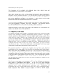 Additionally, if tested on a chassis dynamometer, one risks damaging the dynamometer
and the vehicle's brakes.
19
A graphic of this version of the highway line haul drive cycle is provided below in figure
2.
Figure 2
CO-
CO
JO
|Q •
0
r?
High/vary Line Haul
>Q JO
Another version of a highway line haul cycle, suitable for use only on a chassis
dynamometer, was created by Southwest Research Institute, using input from a group of
stakeholders, including EPA, Northeastern States for Coordinated Air Use Management
(NESCAUM), several truck and engine manufacturers, state organizations, and others,
for a NESCAUM heavy truck fuel efficiency modeling and simulation project. It is
similar to the first option shown above, although top and average speeds are increased,
there are grade impacts, there is less transient operation, and idling is handled in a
separate cycle. A graphic of this version of the highway line haul drive cycle is provided
below in figure 3.
Figure 3
I ,'
SCO
tOOD
2000
2SOO
30DO
3SOO JDOO .1500 5000
24
image:
Additionally, if tested on a chassis dynamometer, one risks damaging the dynamometer
and the vehicle's brakes.
19
A graphic of this version of the highway line haul drive cycle is provided below in figure
2.
Figure 2
CO-
CO
JO
|Q •
0
r?
High/vary Line Haul
>Q JO
Another version of a highway line haul cycle, suitable for use only on a chassis
dynamometer, was created by Southwest Research Institute, using input from a group of
stakeholders, including EPA, Northeastern States for Coordinated Air Use Management
(NESCAUM), several truck and engine manufacturers, state organizations, and others,
for a NESCAUM heavy truck fuel efficiency modeling and simulation project. It is
similar to the first option shown above, although top and average speeds are increased,
there are grade impacts, there is less transient operation, and idling is handled in a
separate cycle. A graphic of this version of the highway line haul drive cycle is provided
below in figure 3.
Figure 3
I ,'
SCO
tOOD
2000
2SOO
30DO
3SOO JDOO .1500 5000
24
image:
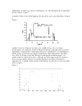 Each of these cycles may be considered, with the potential to combine features of each
into a final Highway Line Haul cycle. Data and input on payload and accessory load will
also be considered, to develop these aspects of the drive cycle (discussed in Section xx).
9.3 Regional Haul
Regional haul operation is similar to highway line haul, the primary distinction being that
regional haul has relatively shorter trip lengths, and includes some suburban-type
operation, with lower average speeds, relatively more frequent congested driving, and no
(or infrequent) overnight stays. If purchased new for this application, the tractor is
typically a day cab, without sleeper accommodation.
EPA is still selecting options for this drive cycle. One promising option is to integrate
segments of the Transient mode of the ARB HHDDT test into the finalized Highway
Line Haul cycle (which is based upon the Cruise module of the ARB HHDDT test), to
create a single drive cycle of sufficient duration and complexity.
Analysis and "filtering" of the ARB Cruise and Transient modes has been conducted by
West Virginia University. This work, combined with input on the line-haul cycle, could
serve as the basis for a regional haul drive cycle. EPA will begin to formalize
recommendations for the regional haul cycle and include specific options in subsequent
drafts of this protocol.
9.4 Local Pick Up and Delivery
The local pick up and delivery cycle simulates a package, parcel, or beverage delivery
truck operating in urban-type driving, to provide local pick up and delivery service to
residences and businesses. This type of truck operation is characterized by very frequent
stops and starts, with limited "stem" highway driving to and from the distribution center.
The vehicles are powered by heavy duty engines typically used in class 4 to 6 trucks
(14,001 to 26,000 pounds GVWR), although some vehicles may be as light as class 2b or
3. The vehicle is typically a single unit truck or a chassis/truck body combination, with 2
axles.
EPA is still collecting information on local pick up and delivery candidate drive cycles.
The parcel delivery working group of the Calstart-Weststart Hybrid Truck Users Forum
(HTUF) instrumented a small number of parcel delivery trucks in the Florida area, and
developed two parcel delivery drive cycles. One represents a class 4 residential delivery
truck, and one represents a class 6 commercial delivery truck. The major differences
between these two drive cycles are the rate of acceleration, average speed, number of
stops, and percent of stops that are idle or engine off.
Graphics of the two parcel delivery drive cycle candidates are provided below in figures
4 and 5.
25
image:
Each of these cycles may be considered, with the potential to combine features of each
into a final Highway Line Haul cycle. Data and input on payload and accessory load will
also be considered, to develop these aspects of the drive cycle (discussed in Section xx).
9.3 Regional Haul
Regional haul operation is similar to highway line haul, the primary distinction being that
regional haul has relatively shorter trip lengths, and includes some suburban-type
operation, with lower average speeds, relatively more frequent congested driving, and no
(or infrequent) overnight stays. If purchased new for this application, the tractor is
typically a day cab, without sleeper accommodation.
EPA is still selecting options for this drive cycle. One promising option is to integrate
segments of the Transient mode of the ARB HHDDT test into the finalized Highway
Line Haul cycle (which is based upon the Cruise module of the ARB HHDDT test), to
create a single drive cycle of sufficient duration and complexity.
Analysis and "filtering" of the ARB Cruise and Transient modes has been conducted by
West Virginia University. This work, combined with input on the line-haul cycle, could
serve as the basis for a regional haul drive cycle. EPA will begin to formalize
recommendations for the regional haul cycle and include specific options in subsequent
drafts of this protocol.
9.4 Local Pick Up and Delivery
The local pick up and delivery cycle simulates a package, parcel, or beverage delivery
truck operating in urban-type driving, to provide local pick up and delivery service to
residences and businesses. This type of truck operation is characterized by very frequent
stops and starts, with limited "stem" highway driving to and from the distribution center.
The vehicles are powered by heavy duty engines typically used in class 4 to 6 trucks
(14,001 to 26,000 pounds GVWR), although some vehicles may be as light as class 2b or
3. The vehicle is typically a single unit truck or a chassis/truck body combination, with 2
axles.
EPA is still collecting information on local pick up and delivery candidate drive cycles.
The parcel delivery working group of the Calstart-Weststart Hybrid Truck Users Forum
(HTUF) instrumented a small number of parcel delivery trucks in the Florida area, and
developed two parcel delivery drive cycles. One represents a class 4 residential delivery
truck, and one represents a class 6 commercial delivery truck. The major differences
between these two drive cycles are the rate of acceleration, average speed, number of
stops, and percent of stops that are idle or engine off.
Graphics of the two parcel delivery drive cycle candidates are provided below in figures
4 and 5.
25
image:
 Figure 4: ~ HTUF Class 4 parcel delivery cycle
Figure 5:~ HTUF Class 6 parcel delivery cycle
HTUF Class 6 PDDS - Full Cycle
1 160 319 478 637 796 955111412731432159117501909206822272386254527042863302231813340349936583817
Time (sec.)
EPA is also instrumenting parcel delivery trucks for its hydraulic hybrid development
program. After this data is collected and analyzed, EPA can determine what changes, if
any, might be made to the HTUF drive cycles, and whether we want one single cycle, or
whether we could develop a formula that allows a testing organization to chose a
weighted combination of more than one cycle, depending upon vehicle service
characteristics. Data and information on payload and accessory load will also be
considered.
26
image:
Figure 4: ~ HTUF Class 4 parcel delivery cycle
Figure 5:~ HTUF Class 6 parcel delivery cycle
HTUF Class 6 PDDS - Full Cycle
1 160 319 478 637 796 955111412731432159117501909206822272386254527042863302231813340349936583817
Time (sec.)
EPA is also instrumenting parcel delivery trucks for its hydraulic hybrid development
program. After this data is collected and analyzed, EPA can determine what changes, if
any, might be made to the HTUF drive cycles, and whether we want one single cycle, or
whether we could develop a formula that allows a testing organization to chose a
weighted combination of more than one cycle, depending upon vehicle service
characteristics. Data and information on payload and accessory load will also be
considered.
26
image:
 9.5 Neighborhood Refuse Truck
The neighborhood refuse truck drive cycle simulates a trash collection and compacting
truck, operating in urban-type driving, to provide residential and commercial solid waste
collection within a local community. The vehicle operation is characterized by very
frequent stops and starts, with limited "stem" highway or suburban driving to and from
the refuse drop-off site. During its operation, the engine or other power source is
typically used to operate hydraulic and/or other lifting, compacting, and dumping
functions. A significant amount of the fuel used by neighborhood refuse trucks is
consumed by these non-motive functions. These vehicles are powered by heavy duty
engines typically used in class 7 or class 8 trucks (greater than 26,001 pounds GVWR).
The typical refuse haul vehicle is a chassis/truck body combination with a single axle
tractor and either a single or tandem axle trash loader/ packer body.
One candidate neighborhood refuse truck drive cycle was developed by the National
Renewable Energy Laboratory of Department of Energy using data collected by Ohio
State University, from instrumented neighborhood refuse trucks in 5 different cities. It
includes vehicle operation during collection, dumping, and driving to and from the dump
and neighborhood sites.
A graphic of this candidate neighborhood refuse truck drive cycle is provided in Figure 6.
Due to the complexity of this refuse hauler cycle, this cycle should be performed on a
heavy duty vehicle chassis dynamometer only.
Figure 6
70
50
Q.
20
10
500
1000
Time (s)
1500
2000
27
image:
9.5 Neighborhood Refuse Truck
The neighborhood refuse truck drive cycle simulates a trash collection and compacting
truck, operating in urban-type driving, to provide residential and commercial solid waste
collection within a local community. The vehicle operation is characterized by very
frequent stops and starts, with limited "stem" highway or suburban driving to and from
the refuse drop-off site. During its operation, the engine or other power source is
typically used to operate hydraulic and/or other lifting, compacting, and dumping
functions. A significant amount of the fuel used by neighborhood refuse trucks is
consumed by these non-motive functions. These vehicles are powered by heavy duty
engines typically used in class 7 or class 8 trucks (greater than 26,001 pounds GVWR).
The typical refuse haul vehicle is a chassis/truck body combination with a single axle
tractor and either a single or tandem axle trash loader/ packer body.
One candidate neighborhood refuse truck drive cycle was developed by the National
Renewable Energy Laboratory of Department of Energy using data collected by Ohio
State University, from instrumented neighborhood refuse trucks in 5 different cities. It
includes vehicle operation during collection, dumping, and driving to and from the dump
and neighborhood sites.
A graphic of this candidate neighborhood refuse truck drive cycle is provided in Figure 6.
Due to the complexity of this refuse hauler cycle, this cycle should be performed on a
heavy duty vehicle chassis dynamometer only.
Figure 6
70
50
Q.
20
10
500
1000
Time (s)
1500
2000
27
image:
 EPA will request stakeholder input on this drive cycle, including payload and accessory
load.
9.6 Utility Service Truck
The utility service truck drive cycle simulates a public utility, cable, or telecom service
truck operating in urban-type driving, to furnish electricity, gas, water, or telephone
service to local businesses and residences by conducting service calls and fixing
"trouble" on utility lines and junctions. Vehicle operation is characterized by periods of
using the engine or other power source to operate hydraulic aerial lifts, and/or to supply
electrical power to the grid and/or to operate on-board equipment. A significant amount
of the fuel used by utility service trucks is consumed during these non-motive functions.
The vehicles are powered by heavy duty engines typically used in class 6 or 7 trucks
(19,501 to 33,000 pounds GVWR). A typical vehicle is a chassis/truck body combination
with a single axle tractor and a single axle truck body equipped with outside-accessible
compartments and a 30' to 50' hydraulic aerial lift (boom) for lifting workers and tools.
A potential utility service truck cycle is the CILCC drive cycle, a composite cycle
developed by DOE/NREL, Eaton, and International Truck and Engine. These
organizations developed their cycle by extensive and iterative analysis that compared
several candidate drive cycles against key performance needs of hybrid electric urban
delivery vehicles. Eaton and Southwest Research Institute have used this cycle in their
fuel efficiency tests of hybrid utility service trucks.
Eaton and SwRI also developed hydraulic and electric test cycles to measure power
demand for the aerial lift and powering the grid, which could be incorporated into this
cycle, along with payload requirements.
The CILCC cycle is shown below, in figure 7.
28
image:
EPA will request stakeholder input on this drive cycle, including payload and accessory
load.
9.6 Utility Service Truck
The utility service truck drive cycle simulates a public utility, cable, or telecom service
truck operating in urban-type driving, to furnish electricity, gas, water, or telephone
service to local businesses and residences by conducting service calls and fixing
"trouble" on utility lines and junctions. Vehicle operation is characterized by periods of
using the engine or other power source to operate hydraulic aerial lifts, and/or to supply
electrical power to the grid and/or to operate on-board equipment. A significant amount
of the fuel used by utility service trucks is consumed during these non-motive functions.
The vehicles are powered by heavy duty engines typically used in class 6 or 7 trucks
(19,501 to 33,000 pounds GVWR). A typical vehicle is a chassis/truck body combination
with a single axle tractor and a single axle truck body equipped with outside-accessible
compartments and a 30' to 50' hydraulic aerial lift (boom) for lifting workers and tools.
A potential utility service truck cycle is the CILCC drive cycle, a composite cycle
developed by DOE/NREL, Eaton, and International Truck and Engine. These
organizations developed their cycle by extensive and iterative analysis that compared
several candidate drive cycles against key performance needs of hybrid electric urban
delivery vehicles. Eaton and Southwest Research Institute have used this cycle in their
fuel efficiency tests of hybrid utility service trucks.
Eaton and SwRI also developed hydraulic and electric test cycles to measure power
demand for the aerial lift and powering the grid, which could be incorporated into this
cycle, along with payload requirements.
The CILCC cycle is shown below, in figure 7.
28
image:
 LL-Li
j_
"o TO IITC 1500
Figure 7
9.7 Transit Bus
The transit bus cycle simulates a 35' to 40' bus operating primarily in local areas, to
provide frequent-stop passenger service. This vehicle operation is characterized by low
average speed and regular, frequent stops, with relatively short trip lengths between
stops. Vehicles typically lack facilities for long-distance operation (e.g., no onboard
restrooms or large luggage compartments). However, passenger comfort and information
is essential. Transit buses use the engine or other power source to power internal and
external signs, interior lighting, and hydraulic lifts, and to supply heat, ventilation, and air
conditioning (HVAC). A significant amount of the fuel used by transit buses is
consumed by these non-motive "hotel loads." They are powered by heavy duty engines
typically used in class 7 or 8 trucks (over 26,000 pounds GVWR). A typical transit bus is
a single body construction with 2 axles. It can accommodate over 15 passengers, and is
equipped with 2 sets of doors.
There are significant differences between transit buses operating in suburban
neighborhoods, and transit buses operating in more urban neighborhoods. In recognition
of the differences, two different candidate drive cycles may be chosen for testing transit
buses: the Manhattan bus cycle and Orange County bus cycle, representing urban and
suburban transit service, respectively.
The Manhattan Bus Cycle was developed based upon the driving patterns of buses in the
Manhattan core of New York City. The cycle, originally published as a transient chassis
dynamometer test cycle for urban transit buses, is characterized by frequent stops and
very low speed. The maximum speed is 25.4 mph; the average speed is 6.8 mph
(ll.Okm/h).
The Orange County Bus Cycle was developed by West Virginia University based upon
the driving patterns of urban transit buses in the Los Angeles area. The cycle, originally
29
image:
LL-Li
j_
"o TO IITC 1500
Figure 7
9.7 Transit Bus
The transit bus cycle simulates a 35' to 40' bus operating primarily in local areas, to
provide frequent-stop passenger service. This vehicle operation is characterized by low
average speed and regular, frequent stops, with relatively short trip lengths between
stops. Vehicles typically lack facilities for long-distance operation (e.g., no onboard
restrooms or large luggage compartments). However, passenger comfort and information
is essential. Transit buses use the engine or other power source to power internal and
external signs, interior lighting, and hydraulic lifts, and to supply heat, ventilation, and air
conditioning (HVAC). A significant amount of the fuel used by transit buses is
consumed by these non-motive "hotel loads." They are powered by heavy duty engines
typically used in class 7 or 8 trucks (over 26,000 pounds GVWR). A typical transit bus is
a single body construction with 2 axles. It can accommodate over 15 passengers, and is
equipped with 2 sets of doors.
There are significant differences between transit buses operating in suburban
neighborhoods, and transit buses operating in more urban neighborhoods. In recognition
of the differences, two different candidate drive cycles may be chosen for testing transit
buses: the Manhattan bus cycle and Orange County bus cycle, representing urban and
suburban transit service, respectively.
The Manhattan Bus Cycle was developed based upon the driving patterns of buses in the
Manhattan core of New York City. The cycle, originally published as a transient chassis
dynamometer test cycle for urban transit buses, is characterized by frequent stops and
very low speed. The maximum speed is 25.4 mph; the average speed is 6.8 mph
(ll.Okm/h).
The Orange County Bus Cycle was developed by West Virginia University based upon
the driving patterns of urban transit buses in the Los Angeles area. The cycle, originally
29
image:
 published as a chassis dynamometer test cycle for intermediate speed transit bus
operation, has a maximum speed of 41.4 mph and an average speed of 12.5 mph.
The speed-time points for the Manhattan and the Orange County bus cycles can be found
in Recommended Practice for Measuring Fuel efficiency and Emissions of Hybrid-
Electric and Conventional Heavy duty Vehicles, SAE Surface Vehicle Recommended
Practice J2711. A graphic depicting each of these cycles is found in Figures 8 and 9.
Due to the complexity of these bus drive cycles, these cycles should be performed on a
heavy duty vehicle chassis dynamometer only.
Figure 8: --Orange County Bus Cycle
30
image:
published as a chassis dynamometer test cycle for intermediate speed transit bus
operation, has a maximum speed of 41.4 mph and an average speed of 12.5 mph.
The speed-time points for the Manhattan and the Orange County bus cycles can be found
in Recommended Practice for Measuring Fuel efficiency and Emissions of Hybrid-
Electric and Conventional Heavy duty Vehicles, SAE Surface Vehicle Recommended
Practice J2711. A graphic depicting each of these cycles is found in Figures 8 and 9.
Due to the complexity of these bus drive cycles, these cycles should be performed on a
heavy duty vehicle chassis dynamometer only.
Figure 8: --Orange County Bus Cycle
30
image:
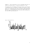 Figure 9: ~ Manhattan Bus Cycle
Determining Which Bus Cycle to Use
Assuming that these candidate cycles are accepted, in order for the selected drive cycle to
be as close to the intended use of the vehicle as possible, there are certain criteria to
determine whether the Manhattan or Orange County drive cycle should be used for a
specific vehicle test.
Two major factors that determine transit bus performance and for which data are readily
available are average route speed and percent idle ("stopped") time. Of these, average
route speed is the most significant discriminator in predicting performance. These two
parameters are combined into an index that determines which of the two drive cycles
shall be used to test the fuel consumption of a specific transit bus model.
The midpoint between the average speeds on the two cycles is 9.58 mph, and the
midpoint of percent idle is 28.5%. In the combination of these two parameters, the
average speed is given twice the weight of percent idle. By equating the ranges of the
two quantities and after normalization the following formula is obtained:
Cycle Index = 0.013 x (percent idle) + 6.025 H- (average speed in mph)
If the cycle index for the proposed average of all anticipated routes is greater than or
equal to 1, the Manhattan cycle shall be used. If the cycle index is less than 1, the Orange
County cycle shall be used.
As an example, the Cycle Index for a bus fleet with a predicted fleet average speed and
idle time exactly that of the Manhattan cycle would be the following:
0.013 x (36) + 6.025/6.83 = 1.35
The Cycle Index for a bus fleet with a predicted fleet average speed and idle time exactly
that of the OCTA cycle would be the following:
0.013 x (21) + 6.025/12.33 = 0.76
31
image:
Figure 9: ~ Manhattan Bus Cycle
Determining Which Bus Cycle to Use
Assuming that these candidate cycles are accepted, in order for the selected drive cycle to
be as close to the intended use of the vehicle as possible, there are certain criteria to
determine whether the Manhattan or Orange County drive cycle should be used for a
specific vehicle test.
Two major factors that determine transit bus performance and for which data are readily
available are average route speed and percent idle ("stopped") time. Of these, average
route speed is the most significant discriminator in predicting performance. These two
parameters are combined into an index that determines which of the two drive cycles
shall be used to test the fuel consumption of a specific transit bus model.
The midpoint between the average speeds on the two cycles is 9.58 mph, and the
midpoint of percent idle is 28.5%. In the combination of these two parameters, the
average speed is given twice the weight of percent idle. By equating the ranges of the
two quantities and after normalization the following formula is obtained:
Cycle Index = 0.013 x (percent idle) + 6.025 H- (average speed in mph)
If the cycle index for the proposed average of all anticipated routes is greater than or
equal to 1, the Manhattan cycle shall be used. If the cycle index is less than 1, the Orange
County cycle shall be used.
As an example, the Cycle Index for a bus fleet with a predicted fleet average speed and
idle time exactly that of the Manhattan cycle would be the following:
0.013 x (36) + 6.025/6.83 = 1.35
The Cycle Index for a bus fleet with a predicted fleet average speed and idle time exactly
that of the OCTA cycle would be the following:
0.013 x (21) + 6.025/12.33 = 0.76
31
image:
 The average predicted route speed used for this analysis is for the buses while in-service,
and does not include driving to begin the route or to return to the depot after the service
has been completed.
In some cases, the intended service for a particular vehicle may be a route that more
closely resembles a combination of the Manhattan Cycle and the Orange County cycle
than it does either one. Users of this test protocol have the option of running a complete
set of tests with each cycle, then reporting the results as a weighted value of the results
from each cycle.
Payload (passengers) and accessory loads for transit buses are significant, especially the
impacts of air conditioning, heating and defrosting. Power can also be required to lower
and raise the bus to accommodate passengers getting on and off, during typical operation.
Load factors need to be determined for the transit bus cycle. Work to define these loads
started during the development of the Recommended Practice for Measuring Fuel
Economy and Emissions of Hybrid-Electric and Conventional Heavy duty Vehicles, SAE
Surface Vehicle Recommended Practice J2711, and should be considered as a starting
basis for continued development of these load factors.
9.8 Intermodal Drayage Truck
The intermodal drayage truck cycle simulates a combination tractor-chassis freight truck
operating in predominantly local, urban-type driving with relatively short trip lengths.
The vehicles provide intermodal cargo drayage by shuttling ocean-going freight
containers among marine terminals, chassis and container depots, rail terminals, and local
consignees. The operations are characterized by periods of extended creep idle or idle
while waiting at distribution hubs, with limited highway and suburban driving between
destinations. Drayage trucks are powered by heavy duty engines typically used in class 8
trucks (33,001 pounds GVWR or greater). Typically, the tractor will have 3 axles. The
chassis is a framework equipped with 2 axles, on which an ocean-going freight container
is loaded. Chassis can have a sliding adjustable center beam to fit containers of either 20
to 28 feet, or containers of 40 to 48 feet. The latter size is more common.
A candidate intermodal drayage truck cycle was developed by the University of Texas
based upon a number of instrumented trucks operating in the Port of Houston area. A
graphic for the cycle is found in Figure 10.
32
image:
The average predicted route speed used for this analysis is for the buses while in-service,
and does not include driving to begin the route or to return to the depot after the service
has been completed.
In some cases, the intended service for a particular vehicle may be a route that more
closely resembles a combination of the Manhattan Cycle and the Orange County cycle
than it does either one. Users of this test protocol have the option of running a complete
set of tests with each cycle, then reporting the results as a weighted value of the results
from each cycle.
Payload (passengers) and accessory loads for transit buses are significant, especially the
impacts of air conditioning, heating and defrosting. Power can also be required to lower
and raise the bus to accommodate passengers getting on and off, during typical operation.
Load factors need to be determined for the transit bus cycle. Work to define these loads
started during the development of the Recommended Practice for Measuring Fuel
Economy and Emissions of Hybrid-Electric and Conventional Heavy duty Vehicles, SAE
Surface Vehicle Recommended Practice J2711, and should be considered as a starting
basis for continued development of these load factors.
9.8 Intermodal Drayage Truck
The intermodal drayage truck cycle simulates a combination tractor-chassis freight truck
operating in predominantly local, urban-type driving with relatively short trip lengths.
The vehicles provide intermodal cargo drayage by shuttling ocean-going freight
containers among marine terminals, chassis and container depots, rail terminals, and local
consignees. The operations are characterized by periods of extended creep idle or idle
while waiting at distribution hubs, with limited highway and suburban driving between
destinations. Drayage trucks are powered by heavy duty engines typically used in class 8
trucks (33,001 pounds GVWR or greater). Typically, the tractor will have 3 axles. The
chassis is a framework equipped with 2 axles, on which an ocean-going freight container
is loaded. Chassis can have a sliding adjustable center beam to fit containers of either 20
to 28 feet, or containers of 40 to 48 feet. The latter size is more common.
A candidate intermodal drayage truck cycle was developed by the University of Texas
based upon a number of instrumented trucks operating in the Port of Houston area. A
graphic for the cycle is found in Figure 10.
32
image:
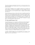 VI
il. n
Figure 10
Additional input and data is needed to refine this drive cycle, including data from other
major port areas (POLB/POLA, NY/NJ), and to develop payload and accessory loads.
10. Accessory Load
Accessory load refers to vehicle power requirements needed to operate equipment,
accessories, and other implements that are essential to the intended vehicle use. These
power requirements are considered a "load" on the engine (or other vehicle power
source), and must be accounted for when evaluating vehicle fuel efficiency. For the
purposes of this test procedure, the following engine/operating components are not
considered "accessories" and the loads will not be measured separately:
• Air compressor
• Water pump
• Engine cooling fan
• Power steering
• Power brakes
The following sections describe the main accessory functions essential to the mission of
many heavy duty vehicles. The power needed to provide these functions must be
accounted for in the fuel efficiency test as an accessory load. The heavy duty fuel
efficiency test protocol will require the following accessory loads be used during a
specific portion of the drive cycle. EPA is still gathering information to determine what
the best options are for including accessory loads and encourages suggestions from
readers of this document. EPA will include those recommended requirements in
subsequent versions of this protocol.
10.1 Heating and Ventilation, Defrosting
Heating and ventilation refers to loads associated with passenger comfort that do not
require operation of the refrigeration cycle of the air conditioner. Heating requires a
source of heat (typically waste heat from the engine cooling system, but not necessarily)
plus operation of a blower motor with air circulation fans. Ventilation requires only
operation of the blower motor and air circulation fans. Defrosting requires a defroster
fan.
33
image:
VI
il. n
Figure 10
Additional input and data is needed to refine this drive cycle, including data from other
major port areas (POLB/POLA, NY/NJ), and to develop payload and accessory loads.
10. Accessory Load
Accessory load refers to vehicle power requirements needed to operate equipment,
accessories, and other implements that are essential to the intended vehicle use. These
power requirements are considered a "load" on the engine (or other vehicle power
source), and must be accounted for when evaluating vehicle fuel efficiency. For the
purposes of this test procedure, the following engine/operating components are not
considered "accessories" and the loads will not be measured separately:
• Air compressor
• Water pump
• Engine cooling fan
• Power steering
• Power brakes
The following sections describe the main accessory functions essential to the mission of
many heavy duty vehicles. The power needed to provide these functions must be
accounted for in the fuel efficiency test as an accessory load. The heavy duty fuel
efficiency test protocol will require the following accessory loads be used during a
specific portion of the drive cycle. EPA is still gathering information to determine what
the best options are for including accessory loads and encourages suggestions from
readers of this document. EPA will include those recommended requirements in
subsequent versions of this protocol.
10.1 Heating and Ventilation, Defrosting
Heating and ventilation refers to loads associated with passenger comfort that do not
require operation of the refrigeration cycle of the air conditioner. Heating requires a
source of heat (typically waste heat from the engine cooling system, but not necessarily)
plus operation of a blower motor with air circulation fans. Ventilation requires only
operation of the blower motor and air circulation fans. Defrosting requires a defroster
fan.
33
image:
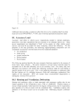 10.2 Air Conditioning
Air conditioning refers to loads associated with passenger comfort that require operation
of the refrigeration cycle of the air conditioner. The air conditioning load may include
the power required to operate a compressor (pump), an evaporator (condenser), and a
blower motor with air circulation fans.
10.3 Power Take-off (PTO) or Other Vocational/Service Work
Load
Power take-off refers to loads associated with the operation of mission functions on a
vocational or service truck. For example, hydraulic load to operate the loading lift arms,
hopper compacting, and dump operations on a neighborhood refuse truck; hydraulic load
to operate the aerial lift on a utility service truck; and, electric load to simulate supplying
electrical power to the grid on a utility service truck.
10.4 Lamps and Lights
Lamps and lights refer to loads associated with the operation of headlights, all other
exterior vehicle lights (tail light, brake light, marker light, hazard light, turn signal light,
license plate light, identification light, clearance light, dome light, etc.), and lights on
instruments and gages.
10.5 Miscellaneous
Refers to accessory loads not otherwise specified, but typical for a given heavy duty
vehicle's operation, including electric windows, electric fuel pump, radio, and electric
wipers.
10.6 Drive Cycle Load Requirements
Work has started to develop accessory load power requirements.20 Substantially more
data and input is needed to determine: 1) the power draw of accessory loads for heavy
duty vehicles; and, 2) the operational characteristics of each heavy duty vehicle, to
determine "typical" hours and intensity of operation for each accessory function. EPA
requests specific comments on drive cycle load requirements for each drive cycle
described above.
Highway Line Haul Accessory Load
[Reserved]
Regional Haul Accessory Load
[Reserved]
34
image:
10.2 Air Conditioning
Air conditioning refers to loads associated with passenger comfort that require operation
of the refrigeration cycle of the air conditioner. The air conditioning load may include
the power required to operate a compressor (pump), an evaporator (condenser), and a
blower motor with air circulation fans.
10.3 Power Take-off (PTO) or Other Vocational/Service Work
Load
Power take-off refers to loads associated with the operation of mission functions on a
vocational or service truck. For example, hydraulic load to operate the loading lift arms,
hopper compacting, and dump operations on a neighborhood refuse truck; hydraulic load
to operate the aerial lift on a utility service truck; and, electric load to simulate supplying
electrical power to the grid on a utility service truck.
10.4 Lamps and Lights
Lamps and lights refer to loads associated with the operation of headlights, all other
exterior vehicle lights (tail light, brake light, marker light, hazard light, turn signal light,
license plate light, identification light, clearance light, dome light, etc.), and lights on
instruments and gages.
10.5 Miscellaneous
Refers to accessory loads not otherwise specified, but typical for a given heavy duty
vehicle's operation, including electric windows, electric fuel pump, radio, and electric
wipers.
10.6 Drive Cycle Load Requirements
Work has started to develop accessory load power requirements.20 Substantially more
data and input is needed to determine: 1) the power draw of accessory loads for heavy
duty vehicles; and, 2) the operational characteristics of each heavy duty vehicle, to
determine "typical" hours and intensity of operation for each accessory function. EPA
requests specific comments on drive cycle load requirements for each drive cycle
described above.
Highway Line Haul Accessory Load
[Reserved]
Regional Haul Accessory Load
[Reserved]
34
image:
 Local Pick Up and Delivery Truck Accessory Load
[Reserved]
Neighborhood Refuse Truck Accessory Load
[Reserved]
Utility Service Truck Accessory Load
[Reserved]
Transit Bus Accessory Load
[Reserved]
Intermodal Drayage Truck Accessory Load
[Reserved]
11. Vehicle Payload and Test Weight
The vehicle test weight is the loaded vehicle weight, as measured at the start of each
complete drive cycle for each vehicle test. This weight shall remain constant for each
drive cycle for the duration of a vehicle test/s. The vehicle test weight is intended to
simulate typical operation for the heavy duty truck application being tested.
Vehicle test weight is generally the vehicle curb weight (weight of empty vehicle without
passengers or payload, but including oil, gas, coolant, and other standard equipment),
plus the weight of the driver, and a specified payload or cargo weight. In the case of a
transit bus, it includes the weight of a specified number of passengers.
The vehicle test weight also includes the weight of the PEMS, plus span and calibration
gases, or the portable fuel tanks, plus test fuel.
For heavy duty vehicles under 14,000 pounds GVWR (up to classS), the vehicle test
weight is the test equivalent weight specified in 40 CFR Part 86, (specifically §86.129-
94).
For all other heavy duty vehicles, a vehicle test weight is stipulated for each of the drive
cycles in this test procedure. The test weights for each drive cycle in this test procedure
are developed taking into consideration vehicle GVWR, typical payload (or other
appropriate weight metrics), average percent empty miles, and weight fluctuation due to
typical cargo loading and unloading patterns.
PAYLOAD VALUES:
21
Highway line haul and regional haul: GVWR is 80,000 pounds. Industry data suggests
an average annual cargo weight of about 36,500 pounds for large over-the-road trucks.
Assuming a typical tractor and enclosed van trailer with a curb weight range from 28,000
35
image:
Local Pick Up and Delivery Truck Accessory Load
[Reserved]
Neighborhood Refuse Truck Accessory Load
[Reserved]
Utility Service Truck Accessory Load
[Reserved]
Transit Bus Accessory Load
[Reserved]
Intermodal Drayage Truck Accessory Load
[Reserved]
11. Vehicle Payload and Test Weight
The vehicle test weight is the loaded vehicle weight, as measured at the start of each
complete drive cycle for each vehicle test. This weight shall remain constant for each
drive cycle for the duration of a vehicle test/s. The vehicle test weight is intended to
simulate typical operation for the heavy duty truck application being tested.
Vehicle test weight is generally the vehicle curb weight (weight of empty vehicle without
passengers or payload, but including oil, gas, coolant, and other standard equipment),
plus the weight of the driver, and a specified payload or cargo weight. In the case of a
transit bus, it includes the weight of a specified number of passengers.
The vehicle test weight also includes the weight of the PEMS, plus span and calibration
gases, or the portable fuel tanks, plus test fuel.
For heavy duty vehicles under 14,000 pounds GVWR (up to classS), the vehicle test
weight is the test equivalent weight specified in 40 CFR Part 86, (specifically §86.129-
94).
For all other heavy duty vehicles, a vehicle test weight is stipulated for each of the drive
cycles in this test procedure. The test weights for each drive cycle in this test procedure
are developed taking into consideration vehicle GVWR, typical payload (or other
appropriate weight metrics), average percent empty miles, and weight fluctuation due to
typical cargo loading and unloading patterns.
PAYLOAD VALUES:
21
Highway line haul and regional haul: GVWR is 80,000 pounds. Industry data suggests
an average annual cargo weight of about 36,500 pounds for large over-the-road trucks.
Assuming a typical tractor and enclosed van trailer with a curb weight range from 28,000
35
image:
 pounds to 32,000 pounds (16,000 to 18,000 pounds for the day cab or sleeper tractor, and
12,000 to 14,000 pounds for the dry van or refrigerated insulated trailer), the cargo
comprises from 70 percent to 76 percent of payload capacity. This information is
summarized in Table xx, below:
Curb Weight Payload GVWR Payload
(tractor & Capacity
trailer)
28,000 36,500 80,000 52,000
30,000 36,500 80,000 50,000
32,000 36,500 80,000 48,000
Percent
Load
70%
73%
76%
Total
Loaded
Weight for
Test
64,500
66,500
68,500
Unused capacity is due to empty hauls, non-revenue miles, and loads that "cube out"
before they "weigh out." Given this range, a recommended payload for testing is 75
percent of payload capacity.
Local pick up and delivery vehicle: GVWR and payload depends upon the intended cargo
and vehicle configuration (parcel, beverage). The vehicle is gradually emptied during the
execution of its duty cycle. A simple approach for a recommended testing payload could
be to consider that the vehicle spends roughly half its miles empty, or a 50 percent
"effective" payload. However, the vehicle may be volume-limited rather than weight-
limited, so the 50 percent would be from volume capacity. More data is needed on
typical payloads for different types of local pick up and delivery vehicles.
Neighborhood refuse truck. GVWR can vary between 52,000 to 72,000 pounds. The
vehicle is gradually filled during the execution of the duty cycle. A simple approach for
a recommended testing payload could be to consider that the vehicle spends roughly half
its miles full, or a 50 percent "effective" payload. However, the vehicle may be volume-
limited rather than weight-limited, so the 50 percent would be indexed from a volume
capacity. More data is needed on typical payloads for different types of neighborhood
refuse trucks.
Utility service truck. GVWR varies between 16,001 and 33,000 pounds. Truck weight
includes the "payload" weight of the aerial lift and other equipment. More data is needed
on GVWR and payload to develop a recommended payload for testing.
Municipal transit bus: Typical GVWR of 19,001 to 26,000 pounds. A suggested
payload for testing is curb weight, plus driver, plus 150 pounds multiplied by one-half the
seated passenger count. This recommendation is from SAE J2711, §6.3.3.22
Intermodal drayage truck: GVWR of 80,000 pounds. Industry data suggests a typical
cargo weight of about 40,000 for ocean-going containers (based upon agricultural loads).
Assuming a tractor, chassis and 40' container with a curb weight of about 32,000 to
34,000 pounds (16,000 to 18,000 pounds for a tractor; 8,000 for a chassis; 8,000 for an
empty container), the cargo comprises about 83 to 87 percent of the remaining 46,000 to
48,000 pounds payload capacity. Assuming that the ocean-going containers are empty
36
image:
pounds to 32,000 pounds (16,000 to 18,000 pounds for the day cab or sleeper tractor, and
12,000 to 14,000 pounds for the dry van or refrigerated insulated trailer), the cargo
comprises from 70 percent to 76 percent of payload capacity. This information is
summarized in Table xx, below:
Curb Weight Payload GVWR Payload
(tractor & Capacity
trailer)
28,000 36,500 80,000 52,000
30,000 36,500 80,000 50,000
32,000 36,500 80,000 48,000
Percent
Load
70%
73%
76%
Total
Loaded
Weight for
Test
64,500
66,500
68,500
Unused capacity is due to empty hauls, non-revenue miles, and loads that "cube out"
before they "weigh out." Given this range, a recommended payload for testing is 75
percent of payload capacity.
Local pick up and delivery vehicle: GVWR and payload depends upon the intended cargo
and vehicle configuration (parcel, beverage). The vehicle is gradually emptied during the
execution of its duty cycle. A simple approach for a recommended testing payload could
be to consider that the vehicle spends roughly half its miles empty, or a 50 percent
"effective" payload. However, the vehicle may be volume-limited rather than weight-
limited, so the 50 percent would be from volume capacity. More data is needed on
typical payloads for different types of local pick up and delivery vehicles.
Neighborhood refuse truck. GVWR can vary between 52,000 to 72,000 pounds. The
vehicle is gradually filled during the execution of the duty cycle. A simple approach for
a recommended testing payload could be to consider that the vehicle spends roughly half
its miles full, or a 50 percent "effective" payload. However, the vehicle may be volume-
limited rather than weight-limited, so the 50 percent would be indexed from a volume
capacity. More data is needed on typical payloads for different types of neighborhood
refuse trucks.
Utility service truck. GVWR varies between 16,001 and 33,000 pounds. Truck weight
includes the "payload" weight of the aerial lift and other equipment. More data is needed
on GVWR and payload to develop a recommended payload for testing.
Municipal transit bus: Typical GVWR of 19,001 to 26,000 pounds. A suggested
payload for testing is curb weight, plus driver, plus 150 pounds multiplied by one-half the
seated passenger count. This recommendation is from SAE J2711, §6.3.3.22
Intermodal drayage truck: GVWR of 80,000 pounds. Industry data suggests a typical
cargo weight of about 40,000 for ocean-going containers (based upon agricultural loads).
Assuming a tractor, chassis and 40' container with a curb weight of about 32,000 to
34,000 pounds (16,000 to 18,000 pounds for a tractor; 8,000 for a chassis; 8,000 for an
empty container), the cargo comprises about 83 to 87 percent of the remaining 46,000 to
48,000 pounds payload capacity. Assuming that the ocean-going containers are empty
36
image:
 for nearly half their trucked miles, this would bring the effective average weight to
20,000 pounds, or about 42 to 43 percent of rated payload. More data is needed on
GVWR and payload to develop a recommended payload for testing.
11.1 Test Equivalent Weight
The test equivalent test weight is the normative weight at which the test shall be
conducted, when using the chassis dynamometer method. This weight is used to
determine dynamometer inertia weight settings. Test equivalent weight is based upon the
vehicle test weight (but not to exceed 250 pounds below the vehicle test weight). For all
heavy duty vehicles above 14,000 pounds GVWR, refer to the following table:
Vehicle Test Weight From Drive Cycle (Ibs) Test Equivalent Test Weight (Ibs)
13,751 to 14,250 14,000
14,251 to 14,750 14,500
14,751 to 15,250 15,000
15,251 to 15,750 15,500
Numerical pattern repeats up to and
including....
80,251 to 80,750 80,500
80,751 to 81, 250 81,000
81,251 to 81,750 81,500
For all heavy duty vehicles below 14,000 pounds, refer to the test equivalent test weights
found in 40 CFR Part 86 (specifically §86.129-94).
11.2 Test Fuel Weight and Volume
In accordance with SAE J1321, maintain fuel volumes as consistently as possible over
the course of the test, to minimize random weight variation.
The amount of test fuel in the vehicle fuel tanks shall be topped off at the beginning of
each test day. Ideally, this will ensure that tests will be conducted with an initial fuel
volume of between 50 and 75 percent of the total capacity of the vehicle fuel tank.
If the fuel efficiency test is conducted using the gravimetric method with portable fuel
tanks, the weight of the portable fuel tanks including fuel must be considered in loading
the vehicle to its required test weight.
37
image:
for nearly half their trucked miles, this would bring the effective average weight to
20,000 pounds, or about 42 to 43 percent of rated payload. More data is needed on
GVWR and payload to develop a recommended payload for testing.
11.1 Test Equivalent Weight
The test equivalent test weight is the normative weight at which the test shall be
conducted, when using the chassis dynamometer method. This weight is used to
determine dynamometer inertia weight settings. Test equivalent weight is based upon the
vehicle test weight (but not to exceed 250 pounds below the vehicle test weight). For all
heavy duty vehicles above 14,000 pounds GVWR, refer to the following table:
Vehicle Test Weight From Drive Cycle (Ibs) Test Equivalent Test Weight (Ibs)
13,751 to 14,250 14,000
14,251 to 14,750 14,500
14,751 to 15,250 15,000
15,251 to 15,750 15,500
Numerical pattern repeats up to and
including....
80,251 to 80,750 80,500
80,751 to 81, 250 81,000
81,251 to 81,750 81,500
For all heavy duty vehicles below 14,000 pounds, refer to the test equivalent test weights
found in 40 CFR Part 86 (specifically §86.129-94).
11.2 Test Fuel Weight and Volume
In accordance with SAE J1321, maintain fuel volumes as consistently as possible over
the course of the test, to minimize random weight variation.
The amount of test fuel in the vehicle fuel tanks shall be topped off at the beginning of
each test day. Ideally, this will ensure that tests will be conducted with an initial fuel
volume of between 50 and 75 percent of the total capacity of the vehicle fuel tank.
If the fuel efficiency test is conducted using the gravimetric method with portable fuel
tanks, the weight of the portable fuel tanks including fuel must be considered in loading
the vehicle to its required test weight.
37
image:
 Portable tanks shall be topped off before each test, and the weight recorded as per Section
xx of this test procedure.
12. Test Set-Up Procedure
12.1 TestPayload
Where a test payload is required to meet vehicle test weight requirements, the payload
shall be evenly distributed throughout the trailer (or bus body) and the over-axle loads
must be proportional with federal over-axle weight limits.23 For example, if testing at
80,000 pounds, the payload would be distributed to achieve a weight of 12,000 pounds
over the steer axle, 34,000 pounds over the drive axle, and 34,000 pounds over the trailer
axle. If testing the same vehicle at 65,000 pounds, the payload would be distributed to
achieve a weight of approximately 12,000 over the steer axle (since the payload does not
affect the steer axle that much), 26,500 pounds over the drive axle, and 26,500 pounds
over the trailer axle. It is recommended that the test payload be secured by strapping
down then blocking the payload with nailed-down chucks, so that the payload will not
shift during the test. Payload must not change during a test.
The vehicle must be weighed using properly calibrated truck weight scales that conform
to the most current provisions established by the National Institute of Standards and
Technology (NIST). It is recommended that the truck scales also have a National Type
Evaluation Program (NTEP) Certificate of Conformance.
12.2 Tire Pressure
Tires shall be representative of a typical (e.g., best-selling) tire for a given vehicle
application, unless a special tire characteristic (e.g., low rolling resistance) is a condition
being tested.
Tire pressure shall be adjusted at cold condition as needed before pre conditioning, and
tested to the tire manufacturer's recommended maximum cold inflation pressure. Tire
pressure shall also be measured at the end of each completed test run to ensure that, at a
minimum , the inflation pressure is consistent with the starting cold pressure.
12.3 Mechanical Preparation of Test Vehicle
Vehicles shall be representative of production fleet vehicles. Test vehicles need not be
new, but they must be in good mechanical order and operating condition. All
components and equipment shall be calibrated and maintained to within manufacturer-
recommended specifications. The exception is any component that has been deliberately
modified as part of the test truck design.
Vehicles shall be mechanically prepared and maintained in accordance with SAE J1321,
Sections §8.6 to §8.10. Vehicles must not have any mechanical or physical defects that
38
image:
Portable tanks shall be topped off before each test, and the weight recorded as per Section
xx of this test procedure.
12. Test Set-Up Procedure
12.1 TestPayload
Where a test payload is required to meet vehicle test weight requirements, the payload
shall be evenly distributed throughout the trailer (or bus body) and the over-axle loads
must be proportional with federal over-axle weight limits.23 For example, if testing at
80,000 pounds, the payload would be distributed to achieve a weight of 12,000 pounds
over the steer axle, 34,000 pounds over the drive axle, and 34,000 pounds over the trailer
axle. If testing the same vehicle at 65,000 pounds, the payload would be distributed to
achieve a weight of approximately 12,000 over the steer axle (since the payload does not
affect the steer axle that much), 26,500 pounds over the drive axle, and 26,500 pounds
over the trailer axle. It is recommended that the test payload be secured by strapping
down then blocking the payload with nailed-down chucks, so that the payload will not
shift during the test. Payload must not change during a test.
The vehicle must be weighed using properly calibrated truck weight scales that conform
to the most current provisions established by the National Institute of Standards and
Technology (NIST). It is recommended that the truck scales also have a National Type
Evaluation Program (NTEP) Certificate of Conformance.
12.2 Tire Pressure
Tires shall be representative of a typical (e.g., best-selling) tire for a given vehicle
application, unless a special tire characteristic (e.g., low rolling resistance) is a condition
being tested.
Tire pressure shall be adjusted at cold condition as needed before pre conditioning, and
tested to the tire manufacturer's recommended maximum cold inflation pressure. Tire
pressure shall also be measured at the end of each completed test run to ensure that, at a
minimum , the inflation pressure is consistent with the starting cold pressure.
12.3 Mechanical Preparation of Test Vehicle
Vehicles shall be representative of production fleet vehicles. Test vehicles need not be
new, but they must be in good mechanical order and operating condition. All
components and equipment shall be calibrated and maintained to within manufacturer-
recommended specifications. The exception is any component that has been deliberately
modified as part of the test truck design.
Vehicles shall be mechanically prepared and maintained in accordance with SAE J1321,
Sections §8.6 to §8.10. Vehicles must not have any mechanical or physical defects that
38
image:
 may affect fuel efficiency. Vehicles must not have any fluid, exhaust, or air suspension
leaks. There must be a visual inspection of the tires prior to each test day, to detect any
signs of tire or wheel damage or unusual wear.
The air cleaner monitor and engine fault codes must be checked prior to the test, and any
abnormal conditions must be corrected, to ensure that the vehicle is in proper working
order. It is recommended that the crankcase, differential, and gear lubricant be removed
and replaced with fresh lubricant prior to the test.
Test vehicles shall have accumulated a minimum of 2,500 miles prior to testing (10,000
miles are recommended to properly break in a new vehicle).
If the test method uses the carbon balance method of fuel consumption measurement,
follow the additional vehicle preparation requirements in CFR 40 §86.131-90.
Vehicles must be fueled from the same fuel dispenser during the entire test to ensure
consistent fuel grade and quality. Empty the test fuel tanks by draining, or by vehicle
operation, before filling with test fuel. Refer to CFR 40 §86.132-90. If a removable fuel
tank is being used, it shall be filled only with the test fuel. Refer to Sections §5.7.1,
§5.7.3, and §6.3 of SAE J1321.
If a PEMS is being used, refer to 40 CFR Part 1065 Subpart D for PEMS system set up.
If using the carbon balance method with either a PEMS or laboratory gas analyzers, all
detectable sources of exhaust gas leaks must be sealed or plugged.
Records of vehicle identification and condition must be kept. Refer to SAE J1321 §4 and
the referenced Type II Test Data Forms, and the appendices of this document for more
details. Vehicles must be weighed before the test to ensure proper test weight, and over
axle weighting, and weight records must be maintained.
12.4 Vehicle Preconditioning
Vehicle preconditioning warms the engine and exhaust emission control equipment, and
raises vehicle operating temperatures, so the vehicle is warmed up. Ideally, the engine
coolant, oil and drivetain lubricants should reach an operating temperature that would be
consistent with those expected during multiple repetition of the associated test cycle. To
accomplish these objectives, the test vehicle shall be driven through a warm up cycle
prior to the test. The warm up cycle shall consist of driving the vehicle at least one time
through the drive cycle that will be used for the test, or 60 minutes, whichever is greater.
Hybrid vehicles may require a lengthier warm up time, to establish an equilibrium state
of charge (SOC) in the rechargeable energy storage system (RESS), such that the initial
and final SOC values during the subsequent test cycles will be within the stated tolerance.
Refer to the following sections for more details.
The test shall commence between 10 and 30 minutes after completion of the warm up.
Gas analyzers must be re-calibrated during the interval between warm up and test start.
39
image:
may affect fuel efficiency. Vehicles must not have any fluid, exhaust, or air suspension
leaks. There must be a visual inspection of the tires prior to each test day, to detect any
signs of tire or wheel damage or unusual wear.
The air cleaner monitor and engine fault codes must be checked prior to the test, and any
abnormal conditions must be corrected, to ensure that the vehicle is in proper working
order. It is recommended that the crankcase, differential, and gear lubricant be removed
and replaced with fresh lubricant prior to the test.
Test vehicles shall have accumulated a minimum of 2,500 miles prior to testing (10,000
miles are recommended to properly break in a new vehicle).
If the test method uses the carbon balance method of fuel consumption measurement,
follow the additional vehicle preparation requirements in CFR 40 §86.131-90.
Vehicles must be fueled from the same fuel dispenser during the entire test to ensure
consistent fuel grade and quality. Empty the test fuel tanks by draining, or by vehicle
operation, before filling with test fuel. Refer to CFR 40 §86.132-90. If a removable fuel
tank is being used, it shall be filled only with the test fuel. Refer to Sections §5.7.1,
§5.7.3, and §6.3 of SAE J1321.
If a PEMS is being used, refer to 40 CFR Part 1065 Subpart D for PEMS system set up.
If using the carbon balance method with either a PEMS or laboratory gas analyzers, all
detectable sources of exhaust gas leaks must be sealed or plugged.
Records of vehicle identification and condition must be kept. Refer to SAE J1321 §4 and
the referenced Type II Test Data Forms, and the appendices of this document for more
details. Vehicles must be weighed before the test to ensure proper test weight, and over
axle weighting, and weight records must be maintained.
12.4 Vehicle Preconditioning
Vehicle preconditioning warms the engine and exhaust emission control equipment, and
raises vehicle operating temperatures, so the vehicle is warmed up. Ideally, the engine
coolant, oil and drivetain lubricants should reach an operating temperature that would be
consistent with those expected during multiple repetition of the associated test cycle. To
accomplish these objectives, the test vehicle shall be driven through a warm up cycle
prior to the test. The warm up cycle shall consist of driving the vehicle at least one time
through the drive cycle that will be used for the test, or 60 minutes, whichever is greater.
Hybrid vehicles may require a lengthier warm up time, to establish an equilibrium state
of charge (SOC) in the rechargeable energy storage system (RESS), such that the initial
and final SOC values during the subsequent test cycles will be within the stated tolerance.
Refer to the following sections for more details.
The test shall commence between 10 and 30 minutes after completion of the warm up.
Gas analyzers must be re-calibrated during the interval between warm up and test start.
39
image:
 Intervals between test cycles shall be between 10 and 30 minutes. Gas analyzers shall be
checked after completing the test cycle to ensure that excessive drift hasn't occurred.
If there is any change (i.e., equipment failure or vehicle modification) in the test vehicle
during testing, all testing will be repeated.
For vehicles equipped with a diesel particulate filter, a manual regeneration of the diesel
particulate filter shall be conducted prior to testing.
12.5 Hybrid Vehicles - Additional Vehicle Conditioning
If the vehicle is a hybrid, additional vehicle conditioning is necessary to establish an
"equilibrium" state of charge (SOC) in the rechargeable energy storage system or RESS.
State of charge is a measure of the amount of energy stored in an RESS, expressed as a
percent of the total energy storage capacity of the RESS (battery, flywheel, hydraulic
accumulator, capactor, etc.).
A stable SOC ensures that the energy stored in the RESS will not fluctuate too widely
during the test. If the energy in the storage device fluctuates too widely during a test,
then the amount of energy that the RESS provides to the vehicle relative to total vehicle
fuel consumption will be atypical, and measured vehicle fuel efficiency will not be
representative of that vehicle's true operation. To measure fuel consumption that is
within +/- 3 percent of a vehicle's true, representative fuel consumption, the change in
energy stored in the RESS should be less than +/- 1 percent of the total fuel energy
consumed during a test cycle.24 A stable SOC is within a stated tolerance for the initial
and final SOC values during a test cycle, as described below.
To accomplish this, the hybrid vehicle shall be operated (driven) at least twice through
the drive cycle that will be used for the test in order to verify that the initial and final
SOC values are within the stated tolerance. This vehicle operation can count toward the
requirement for warm-up laps, provided that the test occurs within the time required from
completion of warm up lap.
If the selected drive cycle results in a net increase or decrease in the SOC, then the initial
SOC of the RESS may be adjusted externally following a trial-and-error approach using
the specific procedures detailed below.
If the energy storage capability of the RESS falls below the minimum level specified by
the manufacturer, testing data generated with that vehicle should be discarded and the
vehicle should be repaired or replaced prior to conducting additional testing. (SAE J1711
§4.1.2.3.)
Specific preconditioning information for different types of hybrid vehicles is described
below.
40
image:
Intervals between test cycles shall be between 10 and 30 minutes. Gas analyzers shall be
checked after completing the test cycle to ensure that excessive drift hasn't occurred.
If there is any change (i.e., equipment failure or vehicle modification) in the test vehicle
during testing, all testing will be repeated.
For vehicles equipped with a diesel particulate filter, a manual regeneration of the diesel
particulate filter shall be conducted prior to testing.
12.5 Hybrid Vehicles - Additional Vehicle Conditioning
If the vehicle is a hybrid, additional vehicle conditioning is necessary to establish an
"equilibrium" state of charge (SOC) in the rechargeable energy storage system or RESS.
State of charge is a measure of the amount of energy stored in an RESS, expressed as a
percent of the total energy storage capacity of the RESS (battery, flywheel, hydraulic
accumulator, capactor, etc.).
A stable SOC ensures that the energy stored in the RESS will not fluctuate too widely
during the test. If the energy in the storage device fluctuates too widely during a test,
then the amount of energy that the RESS provides to the vehicle relative to total vehicle
fuel consumption will be atypical, and measured vehicle fuel efficiency will not be
representative of that vehicle's true operation. To measure fuel consumption that is
within +/- 3 percent of a vehicle's true, representative fuel consumption, the change in
energy stored in the RESS should be less than +/- 1 percent of the total fuel energy
consumed during a test cycle.24 A stable SOC is within a stated tolerance for the initial
and final SOC values during a test cycle, as described below.
To accomplish this, the hybrid vehicle shall be operated (driven) at least twice through
the drive cycle that will be used for the test in order to verify that the initial and final
SOC values are within the stated tolerance. This vehicle operation can count toward the
requirement for warm-up laps, provided that the test occurs within the time required from
completion of warm up lap.
If the selected drive cycle results in a net increase or decrease in the SOC, then the initial
SOC of the RESS may be adjusted externally following a trial-and-error approach using
the specific procedures detailed below.
If the energy storage capability of the RESS falls below the minimum level specified by
the manufacturer, testing data generated with that vehicle should be discarded and the
vehicle should be repaired or replaced prior to conducting additional testing. (SAE J1711
§4.1.2.3.)
Specific preconditioning information for different types of hybrid vehicles is described
below.
40
image:
 Hybrid Electric Vehicles with Batteries
Off-vehicle charging of the battery pack is permissible in order to achieve the desired
"equilibrium" SOC.
Hydraulic Hybrid Vehicles
The goal is to have the accumulator pressure at the end of the test be similar to the
accumulator pressure at the start of the test so as to ensure meeting the stated tolerance in
Section 4.6 above. To accomplish this, operate the vehicle over a cycle identical to the
test driving cycle prior to conducting the test. As described above, this vehicle operation
can count toward the requirement for warm-up laps, provided that the test occurs within
the time required from completion of warm up lap.
The hydraulic accumulators can only store about as much energy as is generated over a
typical stop; that energy is usually less than what is needed to accelerate the vehicle for
the next drive event. Therefore, the pressure in the accumulator is dependant on the last
few hills of the drive cycle and is usually at a fairly consistent value at the end of any
drive cycle. A "hill" is a complete start-stop sequence on the drive cycle.
Hybrid Electric Vehicles with Capacitors
Follow a procedure similar to that described for hydraulic hybrid vehicles.
Preconditioning Hybrid Vehicles with Electromechanical Flywheels
Follow a procedure similar to that described for hydraulic hybrid vehicles.
12.6 Hybrid Vehicles - Procedures for Determining State of
Charge (SOC) and Net Energy Change (NEC)
The objective of this protocol is to quantify the fuel efficiency of a vehicle, relative to the
fuel that is consumed. There is to be no net energy provided from the RESS. Thus, the
net energy change (NEC) during a valid test run must be zero, or within a small tolerance
of zero, as defined below.25
In general, the approach to follow, per SAE J2711 §4.3, is to measure the State of Charge
(SOC) at the beginning of the drive cycle/test run, measure the SOC at the end, and
calculate the Net Energy Change as SOCfmai minus SOCmitiai- The NEC is compared to
the Total Cycle Energy (TCE) where TCE is defined as the total fuel energy (TFE) of the
fuel consumed during the test cycle (in consistent units) minus the NEC. The sign
convention for NEC is that negative means that energy was extracted from the RESS
during the test. In that case, the TCE will be larger than the TFE when NEC is negative.
The NEC is calculated as a percentage of the TCE to determine if a test run is valid, can
be made valid with SOC corrections, or is invalid. Follow the procedure outlined in SAE
J1711, §4.3.1.4, with the exception that the selected drive cycle will be used in place of
the HDDS that is cited. More than one drive cycle may be needed to achieve a long
enough test run to achieve the NEC "window", as explained in Section 4.6.
The criteria for the absolute value of the NEC/TCE ratio are as follows:
<1% means the test run is valid and can be used without correction;
41
image:
Hybrid Electric Vehicles with Batteries
Off-vehicle charging of the battery pack is permissible in order to achieve the desired
"equilibrium" SOC.
Hydraulic Hybrid Vehicles
The goal is to have the accumulator pressure at the end of the test be similar to the
accumulator pressure at the start of the test so as to ensure meeting the stated tolerance in
Section 4.6 above. To accomplish this, operate the vehicle over a cycle identical to the
test driving cycle prior to conducting the test. As described above, this vehicle operation
can count toward the requirement for warm-up laps, provided that the test occurs within
the time required from completion of warm up lap.
The hydraulic accumulators can only store about as much energy as is generated over a
typical stop; that energy is usually less than what is needed to accelerate the vehicle for
the next drive event. Therefore, the pressure in the accumulator is dependant on the last
few hills of the drive cycle and is usually at a fairly consistent value at the end of any
drive cycle. A "hill" is a complete start-stop sequence on the drive cycle.
Hybrid Electric Vehicles with Capacitors
Follow a procedure similar to that described for hydraulic hybrid vehicles.
Preconditioning Hybrid Vehicles with Electromechanical Flywheels
Follow a procedure similar to that described for hydraulic hybrid vehicles.
12.6 Hybrid Vehicles - Procedures for Determining State of
Charge (SOC) and Net Energy Change (NEC)
The objective of this protocol is to quantify the fuel efficiency of a vehicle, relative to the
fuel that is consumed. There is to be no net energy provided from the RESS. Thus, the
net energy change (NEC) during a valid test run must be zero, or within a small tolerance
of zero, as defined below.25
In general, the approach to follow, per SAE J2711 §4.3, is to measure the State of Charge
(SOC) at the beginning of the drive cycle/test run, measure the SOC at the end, and
calculate the Net Energy Change as SOCfmai minus SOCmitiai- The NEC is compared to
the Total Cycle Energy (TCE) where TCE is defined as the total fuel energy (TFE) of the
fuel consumed during the test cycle (in consistent units) minus the NEC. The sign
convention for NEC is that negative means that energy was extracted from the RESS
during the test. In that case, the TCE will be larger than the TFE when NEC is negative.
The NEC is calculated as a percentage of the TCE to determine if a test run is valid, can
be made valid with SOC corrections, or is invalid. Follow the procedure outlined in SAE
J1711, §4.3.1.4, with the exception that the selected drive cycle will be used in place of
the HDDS that is cited. More than one drive cycle may be needed to achieve a long
enough test run to achieve the NEC "window", as explained in Section 4.6.
The criteria for the absolute value of the NEC/TCE ratio are as follows:
<1% means the test run is valid and can be used without correction;
41
image:
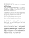 >1% and <5% means that the test run values for emissions and fuel consumption must
have a SOC correction applied to them; and,
>5% means that the test run is invalid.
Achieving runs that fall within this "5-percent window" is a matter of some trial and
error. Preconditioning of the vehicles will be required, as discussed in Section xx. The
drive cycle may be repeated to make a longer test run, if that is advantageous to
achieving the "5-percent window."
Specific procedures for each type of RESS are described in the following sections.
12.6.1 Batteries
The SOC of the battery in a charge-sustaining hybrid electric vehicle can theoretically be
determined by measuring the amp-hours stored, but in practice it is difficult to do with
sufficient accuracy. Thus, for batteries the NEC must be determined indirectly. The
approach is to measure continuously (using a totalizing ammeter) the flow of current into
and out of the battery. The integrated (totalized) value, with the appropriate conversion
factors applied, is the NEC. The specific methodology is shown in SAE J2711, §4.2.1.
Equations 1 and 2. Absolute measures of initial and final SOC will not be available for
the battery; only the net change in stored energy (totalized amp-hours) can be measured.
The correct sign convention must be followed: a negative NEC means a net loss of
charge from the battery.
12.6.2 Capacitors
The SOC for capacitors can be determined with acceptable accuracy by measuring the
voltage across the capacitor pack. Thus the NEC for a test cycle can be readily calculated
by difference of the final and starting SOC. The specific methodology is described in
SAE J2711, §4.2.2, Equation 3.
12.6.3 Electromechanical Flywheels
The SOC for electromechanical flywheels can be determined with acceptable accuracy by
measuring the inertia and speed of the flywheel (revolutions per minute). Thus the NEC
for a test cycle can be readily calculated by difference of the final and starting SOC. The
specific methodology is described in SAE J271 1, §4.2.3, Equation 4.
12.6.4 Hydraulic Accumulators
The SOC for hydraulic accumulators can be determined with acceptable accuracy by
measuring the accumulator pressure (pounds per square inch [psi]). For an accumulator
the SOC can be determined using Equation 1 .
- P*144*FC* —
SOC= - - '- (1)
(l-k)
where:
SOC = State of Charge of the accumulator (Ib-ft)
PC = pre-charge pressure of the accumulator (psi)
42
image:
>1% and <5% means that the test run values for emissions and fuel consumption must
have a SOC correction applied to them; and,
>5% means that the test run is invalid.
Achieving runs that fall within this "5-percent window" is a matter of some trial and
error. Preconditioning of the vehicles will be required, as discussed in Section xx. The
drive cycle may be repeated to make a longer test run, if that is advantageous to
achieving the "5-percent window."
Specific procedures for each type of RESS are described in the following sections.
12.6.1 Batteries
The SOC of the battery in a charge-sustaining hybrid electric vehicle can theoretically be
determined by measuring the amp-hours stored, but in practice it is difficult to do with
sufficient accuracy. Thus, for batteries the NEC must be determined indirectly. The
approach is to measure continuously (using a totalizing ammeter) the flow of current into
and out of the battery. The integrated (totalized) value, with the appropriate conversion
factors applied, is the NEC. The specific methodology is shown in SAE J2711, §4.2.1.
Equations 1 and 2. Absolute measures of initial and final SOC will not be available for
the battery; only the net change in stored energy (totalized amp-hours) can be measured.
The correct sign convention must be followed: a negative NEC means a net loss of
charge from the battery.
12.6.2 Capacitors
The SOC for capacitors can be determined with acceptable accuracy by measuring the
voltage across the capacitor pack. Thus the NEC for a test cycle can be readily calculated
by difference of the final and starting SOC. The specific methodology is described in
SAE J2711, §4.2.2, Equation 3.
12.6.3 Electromechanical Flywheels
The SOC for electromechanical flywheels can be determined with acceptable accuracy by
measuring the inertia and speed of the flywheel (revolutions per minute). Thus the NEC
for a test cycle can be readily calculated by difference of the final and starting SOC. The
specific methodology is described in SAE J271 1, §4.2.3, Equation 4.
12.6.4 Hydraulic Accumulators
The SOC for hydraulic accumulators can be determined with acceptable accuracy by
measuring the accumulator pressure (pounds per square inch [psi]). For an accumulator
the SOC can be determined using Equation 1 .
- P*144*FC* —
SOC= - - '- (1)
(l-k)
where:
SOC = State of Charge of the accumulator (Ib-ft)
PC = pre-charge pressure of the accumulator (psi)
42
image:
 Vc = volume of gas in the accumulator at pre-charge (ft3)
P = current accumulator pressure (psi)
k = ratio of specific heats for the pre-charge gas (1.8 for nitrogen at the high
pressures typical of hydraulic accumulators26).
To convert the units of SOC from Ib-ft to joules, multiply by 1.3558.
The NEC is calculated as the difference in the ending SOC and starting SOC, following a
procedure analogous to that of capacitors and electromechanical flywheels described
above.
12.6.5 SOC Correction and Net Energy Charge
The SOC correction follows the procedure described in SAE J2711, §4.4 that cites a 2000
T7
SAE paper by Clark, et al. A separated SOC correction calculation must be made for
each measured pollutant (if applicable) and for fuel consumption. The measured values
from at least 3 replicate runs are plotted as a function of NEC. A linear regression line is
drawn through the data. If the coefficient of determination, R2, is equal to or greater than
0.80, then the data are acceptable for SOC correction.
Using the regression equation, each y-value (i.e., each individual pollutant emission rate
or the fuel consumption value) is calculated for an x-value (NEC) of zero. These
calculated numbers are the SOC-corrected values that are then used for the comparison
calculations in Section xx.
12.7 Fuel Analysis
A supply of test fuel sufficient to complete the test must be procured and fuel parameters
including fuel density analyzed prior to the start of the test. The test fuel should be
sequestered once it is procured and analyzed. If it is necessary to add additional fuel to
the test fuel supply during the course of the test, another fuel analysis must be conducted
to ensure the test fuel still meets the required fuel parameters. For each test segment, a
record must be kept of the fuel parameters of the test fuel, including density.
The test fuel shall meet fuel specifications summarized in the section of this document
entitled "Test Fuel."
13. Test Procedure
Refer to Figure 11 for an overview of the steps in the overall conduct of the testing, for
either a track or a chassis dynamometer test.
13.1 General Requirements
Driver Conduct
Drivers must be skilled in test driving. Drivers shall be in compliance with existing state
and federal laws governing driver licensing. Generally speaking, a commercial motor
vehicle driver's license or CDL is required in the United States to operate any type of
43
image:
Vc = volume of gas in the accumulator at pre-charge (ft3)
P = current accumulator pressure (psi)
k = ratio of specific heats for the pre-charge gas (1.8 for nitrogen at the high
pressures typical of hydraulic accumulators26).
To convert the units of SOC from Ib-ft to joules, multiply by 1.3558.
The NEC is calculated as the difference in the ending SOC and starting SOC, following a
procedure analogous to that of capacitors and electromechanical flywheels described
above.
12.6.5 SOC Correction and Net Energy Charge
The SOC correction follows the procedure described in SAE J2711, §4.4 that cites a 2000
T7
SAE paper by Clark, et al. A separated SOC correction calculation must be made for
each measured pollutant (if applicable) and for fuel consumption. The measured values
from at least 3 replicate runs are plotted as a function of NEC. A linear regression line is
drawn through the data. If the coefficient of determination, R2, is equal to or greater than
0.80, then the data are acceptable for SOC correction.
Using the regression equation, each y-value (i.e., each individual pollutant emission rate
or the fuel consumption value) is calculated for an x-value (NEC) of zero. These
calculated numbers are the SOC-corrected values that are then used for the comparison
calculations in Section xx.
12.7 Fuel Analysis
A supply of test fuel sufficient to complete the test must be procured and fuel parameters
including fuel density analyzed prior to the start of the test. The test fuel should be
sequestered once it is procured and analyzed. If it is necessary to add additional fuel to
the test fuel supply during the course of the test, another fuel analysis must be conducted
to ensure the test fuel still meets the required fuel parameters. For each test segment, a
record must be kept of the fuel parameters of the test fuel, including density.
The test fuel shall meet fuel specifications summarized in the section of this document
entitled "Test Fuel."
13. Test Procedure
Refer to Figure 11 for an overview of the steps in the overall conduct of the testing, for
either a track or a chassis dynamometer test.
13.1 General Requirements
Driver Conduct
Drivers must be skilled in test driving. Drivers shall be in compliance with existing state
and federal laws governing driver licensing. Generally speaking, a commercial motor
vehicle driver's license or CDL is required in the United States to operate any type of
43
image:
 vehicle with a weight over 26,000 pounds GVWR, including (but not limited to) tow
trucks, tractor trailers and buses. However, these requirements may not apply in all states
and/or on non-public roadways (e.g., a privately-owned test track facility.) It is
recommended that the test facility ensure that all drivers comply with existing state and
federal laws. Pre-determined driving procedures (e.g., gear shifting) shall be specified
prior to the test. Reference SAE J1321 §§5.2 and 5.5. Drivers shall learn the drive cycle
thoroughly prior to the test, and drive test vehicles precisely according to the drive cycle
in terms of required speed at a given time.
Practice runs of the driving cycle are encouraged, to permit driving cycle adjustments and
to allow drivers to learn the drive cycle, so they can meet the speed-time trace accuracy
requirements. Gear-shifting representative of real-world driving shall be encouraged
(neither too smooth nor too aggressive).
For track tests, an observer shall ride in the vehicle with the driver. The observer, using a
stop watch, will coach the driver to meet the target times for each marker, and for the test
overall. The observer will record the actual time to each marker, in accordance with SAE
J1321. Reference SAE J1321 §6.5, and Fuel efficiency Test Forms 2-3 and 2-4.
The same driver (and observer, if applicable) must stay with each vehicle for the duration
of the test.
Track and Chassis Dynamometer Preparation
If the chassis dynamometer has not been used in over two hours prior to the test, it shall
be necessary to warm up the chassis dynamometer for at least 15 minutes prior to the test.
The test vehicle shall not be used for this warm-up. The track shall be prepared for the
specific drive cycle being used by setting up cones, markers, stop signs, and any other
aids to achieve a consistent, repeatable test run. Creating a repeatable test run will be an
iterative process, requiring multiple trial runs.
Fuel Consumption Measurement Equipment Preparation
Follow general specifications for the fuel measurement method selected. For PEMS, use
40 CFR Part 1065, Subparts C and J. For gravimetric/portable fuel tank, use SAE J1321
§§5.7.1 and 5.7.3. For laboratory emissions equipment, use 40 CFR Part 86.315-79.
Section 8 of this document provides more details on each of these fuel measurement
methods.
Additional Steps Required for Hybrid Vehicles
If the vehicle is a hybrid, the RESS SOC should be measured at the start and stop of each
test run. For each different test cycle a minimum of three test runs must be performed to
provide sufficient data for a SOC correction, if needed. It is also recommended that at
least one test run have a net positive and another a net negative NEC value so that net
SOC calculations are based on interpolation and not extrapolation. The NEC must meet
the requirements given in SAE J2711 and vary according to the RESS used.
44
image:
vehicle with a weight over 26,000 pounds GVWR, including (but not limited to) tow
trucks, tractor trailers and buses. However, these requirements may not apply in all states
and/or on non-public roadways (e.g., a privately-owned test track facility.) It is
recommended that the test facility ensure that all drivers comply with existing state and
federal laws. Pre-determined driving procedures (e.g., gear shifting) shall be specified
prior to the test. Reference SAE J1321 §§5.2 and 5.5. Drivers shall learn the drive cycle
thoroughly prior to the test, and drive test vehicles precisely according to the drive cycle
in terms of required speed at a given time.
Practice runs of the driving cycle are encouraged, to permit driving cycle adjustments and
to allow drivers to learn the drive cycle, so they can meet the speed-time trace accuracy
requirements. Gear-shifting representative of real-world driving shall be encouraged
(neither too smooth nor too aggressive).
For track tests, an observer shall ride in the vehicle with the driver. The observer, using a
stop watch, will coach the driver to meet the target times for each marker, and for the test
overall. The observer will record the actual time to each marker, in accordance with SAE
J1321. Reference SAE J1321 §6.5, and Fuel efficiency Test Forms 2-3 and 2-4.
The same driver (and observer, if applicable) must stay with each vehicle for the duration
of the test.
Track and Chassis Dynamometer Preparation
If the chassis dynamometer has not been used in over two hours prior to the test, it shall
be necessary to warm up the chassis dynamometer for at least 15 minutes prior to the test.
The test vehicle shall not be used for this warm-up. The track shall be prepared for the
specific drive cycle being used by setting up cones, markers, stop signs, and any other
aids to achieve a consistent, repeatable test run. Creating a repeatable test run will be an
iterative process, requiring multiple trial runs.
Fuel Consumption Measurement Equipment Preparation
Follow general specifications for the fuel measurement method selected. For PEMS, use
40 CFR Part 1065, Subparts C and J. For gravimetric/portable fuel tank, use SAE J1321
§§5.7.1 and 5.7.3. For laboratory emissions equipment, use 40 CFR Part 86.315-79.
Section 8 of this document provides more details on each of these fuel measurement
methods.
Additional Steps Required for Hybrid Vehicles
If the vehicle is a hybrid, the RESS SOC should be measured at the start and stop of each
test run. For each different test cycle a minimum of three test runs must be performed to
provide sufficient data for a SOC correction, if needed. It is also recommended that at
least one test run have a net positive and another a net negative NEC value so that net
SOC calculations are based on interpolation and not extrapolation. The NEC must meet
the requirements given in SAE J2711 and vary according to the RESS used.
44
image:
 Test Timing
Only "hot start" tests will be used in data reporting and/or data analysis. A hot start is a
test that starts between 10 and 30 minutes of "hot soak" time following a previous test
cycle or preconditioning cycle.
Engine Starting and Restarting
Follow general specifications for starting the vehicle as described in 40 CFR §86.1236-
85.
Drive Trace Accuracy
The test vehicle must be driven according to the drive cycle in terms of required speed at
a given time as closely as possible, to ensure a reproducible test result. The criteria for
determining whether the vehicle met the drive cycle differ for each test method, as
described below. EPA requests comments about whether these accuracy requirements ar
reasonable or necessary.
Track Test Drive Trace Accuracy
The requirements for drive trace accuracy for a track test are adapted from 40 CFR
86.115-78. A test run is considered valid if the driven values fall within the drive cycle
(the "commanded" values) according to the following speed tolerances:
• The upper limit is 2 mph higher than the highest point on the drive cycle, within 1
second of the given time.
• The lower limit is 2 mph lower than the lowest point on the drive cycle, within 1
second of the given time.
Speed variations greater than the tolerances (such as may occur during gear changes or
braking spikes) are acceptable, provided they occur for less than 2 seconds on any
occasion and are clearly documented as to the time and speed at that point of the drive
cycle.
Additionally, to be valid, the total test run shall fall within the ±0.5 percent time
requirement as specified in SAE J1321 §8.5.
Chassis Dynamometer Test Drive Trace Accuracy
The requirements for drive trace accuracy for a chassis dynamometer test are adapted
from SAE J2711, §7.10 using a regression analysis of the "driven" versus the
"commanded" speed at each time point. A test run is considered valid if the slope of the
regression line is between 0.90 and 1.10, and the R-squared value is 0.80 or greater.
Tests that fail to meet this requirement will be deemed invalid.
Running tests in accordance with the light duty vehicle certification procedures in CFR
Part 86 Subpart B also would be considered valid tests.
45
image:
Test Timing
Only "hot start" tests will be used in data reporting and/or data analysis. A hot start is a
test that starts between 10 and 30 minutes of "hot soak" time following a previous test
cycle or preconditioning cycle.
Engine Starting and Restarting
Follow general specifications for starting the vehicle as described in 40 CFR §86.1236-
85.
Drive Trace Accuracy
The test vehicle must be driven according to the drive cycle in terms of required speed at
a given time as closely as possible, to ensure a reproducible test result. The criteria for
determining whether the vehicle met the drive cycle differ for each test method, as
described below. EPA requests comments about whether these accuracy requirements ar
reasonable or necessary.
Track Test Drive Trace Accuracy
The requirements for drive trace accuracy for a track test are adapted from 40 CFR
86.115-78. A test run is considered valid if the driven values fall within the drive cycle
(the "commanded" values) according to the following speed tolerances:
• The upper limit is 2 mph higher than the highest point on the drive cycle, within 1
second of the given time.
• The lower limit is 2 mph lower than the lowest point on the drive cycle, within 1
second of the given time.
Speed variations greater than the tolerances (such as may occur during gear changes or
braking spikes) are acceptable, provided they occur for less than 2 seconds on any
occasion and are clearly documented as to the time and speed at that point of the drive
cycle.
Additionally, to be valid, the total test run shall fall within the ±0.5 percent time
requirement as specified in SAE J1321 §8.5.
Chassis Dynamometer Test Drive Trace Accuracy
The requirements for drive trace accuracy for a chassis dynamometer test are adapted
from SAE J2711, §7.10 using a regression analysis of the "driven" versus the
"commanded" speed at each time point. A test run is considered valid if the slope of the
regression line is between 0.90 and 1.10, and the R-squared value is 0.80 or greater.
Tests that fail to meet this requirement will be deemed invalid.
Running tests in accordance with the light duty vehicle certification procedures in CFR
Part 86 Subpart B also would be considered valid tests.
45
image:
 13.2 Test Procedure for Test Track
Figure 11 below is a general outline of the test sequence for a test conducted on a test
track.
Figure 11. Generic Test Sequence Using Test Track
Conventional and Hybrid Vehicle
Preparation
(pretest measurements,
performance tests, calibrations,
fuel, tires, etc.)
I
Test Track Preparation (cones, stop
signs, etc.)
c
Start
Practice drives
I
Warm-up both test Vehicles
Precondition RESS (hybrid only)
20 - 30 minute (max.)
Hot soak
I
Test Runs
(One or more drive cycles per run)
Repeat, as necessary
(perTest/QA plan, etc.)
to achieve DQO
C
End
Steps to Conduct a Track Test
This test protocol incorporates the test procedure elements outlined in SAE J1321 §§6.1
through 6.9, 6.11, and 6.12. The referenced sections cover details for conducting a test,
which consist of:
46
image:
13.2 Test Procedure for Test Track
Figure 11 below is a general outline of the test sequence for a test conducted on a test
track.
Figure 11. Generic Test Sequence Using Test Track
Conventional and Hybrid Vehicle
Preparation
(pretest measurements,
performance tests, calibrations,
fuel, tires, etc.)
I
Test Track Preparation (cones, stop
signs, etc.)
c
Start
Practice drives
I
Warm-up both test Vehicles
Precondition RESS (hybrid only)
20 - 30 minute (max.)
Hot soak
I
Test Runs
(One or more drive cycles per run)
Repeat, as necessary
(perTest/QA plan, etc.)
to achieve DQO
C
End
Steps to Conduct a Track Test
This test protocol incorporates the test procedure elements outlined in SAE J1321 §§6.1
through 6.9, 6.11, and 6.12. The referenced sections cover details for conducting a test,
which consist of:
46
image:
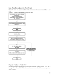 Warm up reference
Ambient condition recording reference
Start of test reference
Initial test run reference
Test run recording and coaching reference
End of test run reference
Interval between test runs reference
Test run repeats reference
One test vehicle, different configurations reference
Two complete test vehicles reference
SAEJ1321 §6.1,
SAEJ1321 §6.2,
SAEJ1321 §6.3,
SAEJ1321 §6.4,
SAEJ1321 §§6.5 and 6.6,
SAEJ1321 §6.7,
SAEJ1321 §6.8,
SAEJ1321 §6.9,
SAEJ1321 §6.11,
SAEJ1321 §6.12.
For §6.8 and 8.13; substitute the phrase "checking data from PEMS" for the word
"refueling" if using the PEMS/carbon balance method instead of the gravimetric method.
13.3 Test Procedure for Chassis Dynamometer
Figure 12 below is a general outline of the test sequence for a test conducted on a chassis
dynamometer.
47
image:
Warm up reference
Ambient condition recording reference
Start of test reference
Initial test run reference
Test run recording and coaching reference
End of test run reference
Interval between test runs reference
Test run repeats reference
One test vehicle, different configurations reference
Two complete test vehicles reference
SAEJ1321 §6.1,
SAEJ1321 §6.2,
SAEJ1321 §6.3,
SAEJ1321 §6.4,
SAEJ1321 §§6.5 and 6.6,
SAEJ1321 §6.7,
SAEJ1321 §6.8,
SAEJ1321 §6.9,
SAEJ1321 §6.11,
SAEJ1321 §6.12.
For §6.8 and 8.13; substitute the phrase "checking data from PEMS" for the word
"refueling" if using the PEMS/carbon balance method instead of the gravimetric method.
13.3 Test Procedure for Chassis Dynamometer
Figure 12 below is a general outline of the test sequence for a test conducted on a chassis
dynamometer.
47
image:
 Figure 12. Generic Test Sequence Using Chassis Dynamometer
Vehicle Preparation (pretest
measurements, performance tests,
calibrations, fuel, tires, etc.)
Start
Practice following drive cycle on
dynamometer
Precondition RESS (hybrid only)
20 - 30 minute (max.)
Hot soak
Test Runs
(One or more drive cycles per run)
Repeat, as necessary
(per test/QA plan, etc.)
to achieve DQO
c
End
Steps to Conduct a Chassis Dynamometer Test
This test protocol incorporates the test procedure elements outlined in 40 CFR Part 86,
Subpart B. Although Subpart B is written for light duty certification procedures, the
steps in Subpart B are in principle the same for performing heavy duty chassis
dynamometer runs.
48
image:
Figure 12. Generic Test Sequence Using Chassis Dynamometer
Vehicle Preparation (pretest
measurements, performance tests,
calibrations, fuel, tires, etc.)
Start
Practice following drive cycle on
dynamometer
Precondition RESS (hybrid only)
20 - 30 minute (max.)
Hot soak
Test Runs
(One or more drive cycles per run)
Repeat, as necessary
(per test/QA plan, etc.)
to achieve DQO
c
End
Steps to Conduct a Chassis Dynamometer Test
This test protocol incorporates the test procedure elements outlined in 40 CFR Part 86,
Subpart B. Although Subpart B is written for light duty certification procedures, the
steps in Subpart B are in principle the same for performing heavy duty chassis
dynamometer runs.
48
image:
 Certain aspects of Subpart B shall be modified for this test. For example, the
dynamometer roll specifications per 86.108-00 will differ for heavy duty chassis
dynamometer rolls.
References in Subpart B to FTP driving schedules and provisions dealing with
evaporative emission testing, the OBD requirements, and the smoke emission
requirements do not apply.
13.4 Coastdown Test Procedure to Calculate Road Load
When conducting a fuel efficiency test using a chassis dynamometer, coast down testing
needs to be conducted to supply road load inputs to the chassis dynamometer. The
vehicle must be tested at its test weight including the payload specified for that drive
cycle.
Depending upon the type of chassis dynamometer used, the appropriate choice of SAE
coast down test shall be conducted: SAE J1263, SAE J2263, or SAE J2264.28 Refer to
these coastdown procedures for details. For example, if a single roll electric
dynamometer is used, J2264 is the appropriate coastdown procedure.
49
image:
Certain aspects of Subpart B shall be modified for this test. For example, the
dynamometer roll specifications per 86.108-00 will differ for heavy duty chassis
dynamometer rolls.
References in Subpart B to FTP driving schedules and provisions dealing with
evaporative emission testing, the OBD requirements, and the smoke emission
requirements do not apply.
13.4 Coastdown Test Procedure to Calculate Road Load
When conducting a fuel efficiency test using a chassis dynamometer, coast down testing
needs to be conducted to supply road load inputs to the chassis dynamometer. The
vehicle must be tested at its test weight including the payload specified for that drive
cycle.
Depending upon the type of chassis dynamometer used, the appropriate choice of SAE
coast down test shall be conducted: SAE J1263, SAE J2263, or SAE J2264.28 Refer to
these coastdown procedures for details. For example, if a single roll electric
dynamometer is used, J2264 is the appropriate coastdown procedure.
49
image:
 14 Required Number of Test Runs
Multiple tests will be needed to establish whether a vehicle meets the performance
standard for a SmartWay designation, as test to test variability (precision) will affect the
results of any single test. We expect that precision will be lower for a track test than for
the dynamometer tests, but in both cases, statistical data will be developed to compute the
required number of tests to provide confidence that the vehicle meets the performance-
based designation. The criterion for meeting this designation is an 80 percent probability
that the test results exceed the fuel efficiency designation by an amount equal to the
lower tail of the 95 percent confidence interval of the test measurements. For example, if
the performance based designation of a particular type of truck was 7.5 miles per gallon,
and replicate measurements showed that the 95 percent confidence interval for the test
was 0.05 miles per gallon, then the results of the statistical computation described below
and in Appendix I should provide evidence of an 80 percent probability that the test result
was 7.5 mile per gallon or greater.
The specific values underlying the statistical assumptions and statistical farmulae are
different will be slightly different for track and dynamomter test data, and these are
presented below and in Appendix I. [A note to rqeaders: We invite comment on this
method.] It is important to note that the following statistical techniques are relevant to
conducting the testing against a known environmental reference truck (discussed in
Purpose and Scope section on page 6 of this document). Testing against an
environmental reference can minimize the number of tests needed to produce appropriate
confidence in the test results.
14.1 General Requirements
The number of tests required for fuel efficiency and emission testing is determined from
the following criteria:
1. A minimum of three (3) tests are required to provide the basic result of a mean
emission reduction and 95 percent confidence interval on that mean based on measured
variability for each of the measurements and test parameters.
2. Additional tests may be required to meet the requirement that the vehicle meets the
performance criterion. These criteria become controlling for low carbon emission/fuel
consumption reductions and/or high test variability. The procedure to determine the
appropriate number of tests is given in the following sections, with additional information
in Appendix I
3. Additional tests may be desired by the applicant to reduce the width of the 95 percent
confidence interval on the mean carbon emission/fuel consumption reduction. Appendix
I provides additional explanation and example scenarios. This third criterion is a
consequence of applying standard statistical procedures to the test design and data
analysis. At fixed measurement variability, normal statistical procedures lead to a small
number of tests giving a broader 95 percent confidence interval than a larger number of
tests. To any potential technology user, a reported reduction in emissions/fuel
consumption of 40 percent ± 5 percent is better than a reported value of 40 percent ± 20
percent, and will be given more credence.
50
image:
14 Required Number of Test Runs
Multiple tests will be needed to establish whether a vehicle meets the performance
standard for a SmartWay designation, as test to test variability (precision) will affect the
results of any single test. We expect that precision will be lower for a track test than for
the dynamometer tests, but in both cases, statistical data will be developed to compute the
required number of tests to provide confidence that the vehicle meets the performance-
based designation. The criterion for meeting this designation is an 80 percent probability
that the test results exceed the fuel efficiency designation by an amount equal to the
lower tail of the 95 percent confidence interval of the test measurements. For example, if
the performance based designation of a particular type of truck was 7.5 miles per gallon,
and replicate measurements showed that the 95 percent confidence interval for the test
was 0.05 miles per gallon, then the results of the statistical computation described below
and in Appendix I should provide evidence of an 80 percent probability that the test result
was 7.5 mile per gallon or greater.
The specific values underlying the statistical assumptions and statistical farmulae are
different will be slightly different for track and dynamomter test data, and these are
presented below and in Appendix I. [A note to rqeaders: We invite comment on this
method.] It is important to note that the following statistical techniques are relevant to
conducting the testing against a known environmental reference truck (discussed in
Purpose and Scope section on page 6 of this document). Testing against an
environmental reference can minimize the number of tests needed to produce appropriate
confidence in the test results.
14.1 General Requirements
The number of tests required for fuel efficiency and emission testing is determined from
the following criteria:
1. A minimum of three (3) tests are required to provide the basic result of a mean
emission reduction and 95 percent confidence interval on that mean based on measured
variability for each of the measurements and test parameters.
2. Additional tests may be required to meet the requirement that the vehicle meets the
performance criterion. These criteria become controlling for low carbon emission/fuel
consumption reductions and/or high test variability. The procedure to determine the
appropriate number of tests is given in the following sections, with additional information
in Appendix I
3. Additional tests may be desired by the applicant to reduce the width of the 95 percent
confidence interval on the mean carbon emission/fuel consumption reduction. Appendix
I provides additional explanation and example scenarios. This third criterion is a
consequence of applying standard statistical procedures to the test design and data
analysis. At fixed measurement variability, normal statistical procedures lead to a small
number of tests giving a broader 95 percent confidence interval than a larger number of
tests. To any potential technology user, a reported reduction in emissions/fuel
consumption of 40 percent ± 5 percent is better than a reported value of 40 percent ± 20
percent, and will be given more credence.
50
image:
 Confidence Interval on the Result
A consequence of the unavoidable variability in test measurements is that the mean of a
small number of measurements has a small probability of giving the true fuel
consumption/emission reduction. In some cases it may not be possible to make a
statistically-significant determination that the measured reduction is different from zero.
The results of measurements conducted using this protocol will be presented as the mean
and 95% confidence interval on that mean, calculated using the sample standard
deviations determined from the test data. Because sample standard deviations are
available, the t-statistic is applied to compute the confidence intervals (as opposed to the
"z" statistic that was used for the sample size calculation).
14.2 Number of Test Runs for Test Track Test
This protocol requires that sufficient tests be conducted to have an 80 percent probability
of detecting whether the fuel efficiency meets or exceeds the performance standard,
computed from the expected experimental variability for the various measurements. In
this context, "detecting" means that the performance standard is less than or equal to the
lower tail of the 95 percent confidence interval. Insufficient replication can result in
inability to detect a statistically significant fuel consumption benefit.
A sample-size equation was derived to explicitly compute the number of tests required
for normally distributed measurements having known standard deviations. However,
since the actual testing procedure will be based on sample standard deviations and t-
statistics, a correction factor was applied to the sample-size equation to account for the
extra variation in the t-distribution relative to that of the normal distribution. Some
results of applying that calculation are presented in Table 1 for emission reductions and
fuel efficiency increases. Equations used to compute the number of tests required are
presented in Appendix I.
Table xx presents the variability of emissions (in this example, NOx), and fuel efficiency
measurements based on standard deviations calculated from an analysis of actual test
track data of Kenworth truck tractors driving a suburban drive cycle.29 The results in
Table 1 are based on the sample-size equation with the correction factor for the one-tailed
t-distribution. More tests than are shown in Table 1 may be required under conditions of
higher variability.
The column headings in the first row of the table give the assumption that the hybrid
vehicle will show an emission reduction or a fuel efficiency improvement of 5 percent,
20 percent, 50 percent, or 85 percent from the baseline conventional emission/fuel
efficiency levels. In developing the Test/QA plan, selection of this value will be based
on the applicant's experience and expectation. The second row gives the constant and
known baseline conventional vehicle variability. The third row is the assumed
measurement variability for the hybrid vehicle based on the variability of the
conventional vehicle. (Variability is expressed as the known standard deviation at the
emission/fuel efficiency level divided by the corresponding conventional vehicle mean
emission/fuel efficiency level and multiplied by 100 percent.) The fourth row gives the
51
image:
Confidence Interval on the Result
A consequence of the unavoidable variability in test measurements is that the mean of a
small number of measurements has a small probability of giving the true fuel
consumption/emission reduction. In some cases it may not be possible to make a
statistically-significant determination that the measured reduction is different from zero.
The results of measurements conducted using this protocol will be presented as the mean
and 95% confidence interval on that mean, calculated using the sample standard
deviations determined from the test data. Because sample standard deviations are
available, the t-statistic is applied to compute the confidence intervals (as opposed to the
"z" statistic that was used for the sample size calculation).
14.2 Number of Test Runs for Test Track Test
This protocol requires that sufficient tests be conducted to have an 80 percent probability
of detecting whether the fuel efficiency meets or exceeds the performance standard,
computed from the expected experimental variability for the various measurements. In
this context, "detecting" means that the performance standard is less than or equal to the
lower tail of the 95 percent confidence interval. Insufficient replication can result in
inability to detect a statistically significant fuel consumption benefit.
A sample-size equation was derived to explicitly compute the number of tests required
for normally distributed measurements having known standard deviations. However,
since the actual testing procedure will be based on sample standard deviations and t-
statistics, a correction factor was applied to the sample-size equation to account for the
extra variation in the t-distribution relative to that of the normal distribution. Some
results of applying that calculation are presented in Table 1 for emission reductions and
fuel efficiency increases. Equations used to compute the number of tests required are
presented in Appendix I.
Table xx presents the variability of emissions (in this example, NOx), and fuel efficiency
measurements based on standard deviations calculated from an analysis of actual test
track data of Kenworth truck tractors driving a suburban drive cycle.29 The results in
Table 1 are based on the sample-size equation with the correction factor for the one-tailed
t-distribution. More tests than are shown in Table 1 may be required under conditions of
higher variability.
The column headings in the first row of the table give the assumption that the hybrid
vehicle will show an emission reduction or a fuel efficiency improvement of 5 percent,
20 percent, 50 percent, or 85 percent from the baseline conventional emission/fuel
efficiency levels. In developing the Test/QA plan, selection of this value will be based
on the applicant's experience and expectation. The second row gives the constant and
known baseline conventional vehicle variability. The third row is the assumed
measurement variability for the hybrid vehicle based on the variability of the
conventional vehicle. (Variability is expressed as the known standard deviation at the
emission/fuel efficiency level divided by the corresponding conventional vehicle mean
emission/fuel efficiency level and multiplied by 100 percent.) The fourth row gives the
51
image:
 calculated number of tests required to have 80 percent probability that the 95 percent
confidence interval about the mean expected emission reduction or fuel efficiency
improvement would not include zero.
Table x. Number of replicate test track tests (for both conventional and hybrid vehicle)
to achieve an 80 percent probability of detecting emission reductions and fuel
efficiency improvements at a confidence level of 95 percent
Expected emission reduction or fuel efficiency
improvement
Variability for baseline conventional vehicle NOX
measurement13
Variability for hybrid vehicle NOX measurement
(assumed to be same as for conventional vehicle)
Number of tests required to have 80 percent probability
of detecting expected NOx emission reduction11
Variability for baseline conventional vehicle fuel
efficiency measurement (MPG)b
Variability for hybrid vehicle fuel efficiency
measurement (MPG) (assumed to be same as for
baseline conventional vehicle)
Number of tests required to have 80 percent probability
of detecting expected fuel efficiency improvement21
5%
2.58%
2.58%
5
2.46%
2.46%
5
20%
2.58%
2.58%
2
2.46%
2.46%
2
50%
2.58%
2.58%
2
2.46%
2.46%
2
85%
2.58%
2.58%
2
2.46%
2.46%
2
Computed under the assumption of normally distributed measurements having known variability.
Additional tests may be required if sample standard deviations obtained during testing are higher.
Computed from standard deviation values from actual track testing of diesel trucks. Citation:
The fifth through the seventh rows (shaded) repeat the calculation for the fuel efficiency
measurement. Table 1 shows that, for both NOX and fuel efficiency, six tests are
sufficient to distinguish between zero and emission reductions/fuel efficiency
improvements as low as 5 percent, based on the assumption that the variability values in
Table x represent the true variability values. Two tests would be sufficient to detect the
other emission reductions/fuel efficiency improvements, but three are required by this
protocol to provide a measured standard deviation.
14.3 Number of Test Runs for Chassis Dynamometer Test
This protocol requires that sufficient tests be conducted to have a high probability of
detecting the emission reductions/fuel efficiency improvements expected by the
applicant. This requirement was implemented to ensure, as much as was practical, that
the test program will accomplish the applicant's goals. This requirement will generally
52
image:
calculated number of tests required to have 80 percent probability that the 95 percent
confidence interval about the mean expected emission reduction or fuel efficiency
improvement would not include zero.
Table x. Number of replicate test track tests (for both conventional and hybrid vehicle)
to achieve an 80 percent probability of detecting emission reductions and fuel
efficiency improvements at a confidence level of 95 percent
Expected emission reduction or fuel efficiency
improvement
Variability for baseline conventional vehicle NOX
measurement13
Variability for hybrid vehicle NOX measurement
(assumed to be same as for conventional vehicle)
Number of tests required to have 80 percent probability
of detecting expected NOx emission reduction11
Variability for baseline conventional vehicle fuel
efficiency measurement (MPG)b
Variability for hybrid vehicle fuel efficiency
measurement (MPG) (assumed to be same as for
baseline conventional vehicle)
Number of tests required to have 80 percent probability
of detecting expected fuel efficiency improvement21
5%
2.58%
2.58%
5
2.46%
2.46%
5
20%
2.58%
2.58%
2
2.46%
2.46%
2
50%
2.58%
2.58%
2
2.46%
2.46%
2
85%
2.58%
2.58%
2
2.46%
2.46%
2
Computed under the assumption of normally distributed measurements having known variability.
Additional tests may be required if sample standard deviations obtained during testing are higher.
Computed from standard deviation values from actual track testing of diesel trucks. Citation:
The fifth through the seventh rows (shaded) repeat the calculation for the fuel efficiency
measurement. Table 1 shows that, for both NOX and fuel efficiency, six tests are
sufficient to distinguish between zero and emission reductions/fuel efficiency
improvements as low as 5 percent, based on the assumption that the variability values in
Table x represent the true variability values. Two tests would be sufficient to detect the
other emission reductions/fuel efficiency improvements, but three are required by this
protocol to provide a measured standard deviation.
14.3 Number of Test Runs for Chassis Dynamometer Test
This protocol requires that sufficient tests be conducted to have a high probability of
detecting the emission reductions/fuel efficiency improvements expected by the
applicant. This requirement was implemented to ensure, as much as was practical, that
the test program will accomplish the applicant's goals. This requirement will generally
52
image:
 only be important to testing intended to measure low emission reductions/fuel efficiency
improvements and/or measurements having high variability.
Specifically, the test program is to be designed such that there is an 80% probability of
detecting the emission reductions/fuel efficiency improvements expected by the
applicant, computed from the expected experimental variability for the various
measurements. In this context, "detecting" means that the 95% confidence interval does
not include zero emissions reduction or zero fuel efficiency improvement. Insufficient
replication can result in inability to detect a statistically significant benefit of a change in
fuel consumption, as illustrated below with a specific example of a hybrid technology.
A sample-size equation was derived to explicitly compute the number of tests required
for normally distributed measurements having known standard deviations. However,
since the actual testing procedure will be based on sample standard deviations and t-
statistics, a correction factor was applied to the sample-size equation to account for the
extra variation in the t-distribution relative to that of the normal distribution. Some
results of applying that calculation are presented in Table 2 for particulate matter (PM)
and NOX emission reductions. The equation used to compute the number of tests required
is presented in Appendix C.
In Table 2 the baseline conventional vehicle is assumed to be operating at a fixed
emission value for PM (top half of table) and NOx (bottom three rows). PM and NOX
measurements are used in Table 2 because dynamometer laboratory-based measurement
standard deviations were known from previous work. The results in Table 2 are based on
the sample-size equation with the correction factor for the t-distribution. More tests than
shown in Table 2 may be required under conditions of higher variability, and careful
examination of the number of tests needed will be required during test/QA plan
development.
The column headings in the first row of the PM and NOX sections of the table give the
assumption that the hybrid vehicle will show emissions reductions of 5%, 20%, 50%, or
85% from the baseline conventional vehicle emissions levels. In developing the Test/QA
plan, selection of this value will be based on the applicant's experience and expectation.
The second row gives the constant and known baseline conventional vehicle variability.
The third row is the assumed measurement variability for the hybrid vehicle based on the
variability of the conventional vehicle. (Variability is expressed as the known standard
deviation at the emission level divided by the corresponding conventional vehicle mean
emission and multiplied by 100%.) The fourth row gives the calculated number of tests
required to have 80% probability that the 95% confidence interval about the mean
expected emission reduction would not include zero.
Table xx. Number of replicate chassis dynamometer tests (for both conventional and
hybrid vehicle) to achieve an 80% probability of detecting emission
reductions at a confidence level of 95%
53
image:
only be important to testing intended to measure low emission reductions/fuel efficiency
improvements and/or measurements having high variability.
Specifically, the test program is to be designed such that there is an 80% probability of
detecting the emission reductions/fuel efficiency improvements expected by the
applicant, computed from the expected experimental variability for the various
measurements. In this context, "detecting" means that the 95% confidence interval does
not include zero emissions reduction or zero fuel efficiency improvement. Insufficient
replication can result in inability to detect a statistically significant benefit of a change in
fuel consumption, as illustrated below with a specific example of a hybrid technology.
A sample-size equation was derived to explicitly compute the number of tests required
for normally distributed measurements having known standard deviations. However,
since the actual testing procedure will be based on sample standard deviations and t-
statistics, a correction factor was applied to the sample-size equation to account for the
extra variation in the t-distribution relative to that of the normal distribution. Some
results of applying that calculation are presented in Table 2 for particulate matter (PM)
and NOX emission reductions. The equation used to compute the number of tests required
is presented in Appendix C.
In Table 2 the baseline conventional vehicle is assumed to be operating at a fixed
emission value for PM (top half of table) and NOx (bottom three rows). PM and NOX
measurements are used in Table 2 because dynamometer laboratory-based measurement
standard deviations were known from previous work. The results in Table 2 are based on
the sample-size equation with the correction factor for the t-distribution. More tests than
shown in Table 2 may be required under conditions of higher variability, and careful
examination of the number of tests needed will be required during test/QA plan
development.
The column headings in the first row of the PM and NOX sections of the table give the
assumption that the hybrid vehicle will show emissions reductions of 5%, 20%, 50%, or
85% from the baseline conventional vehicle emissions levels. In developing the Test/QA
plan, selection of this value will be based on the applicant's experience and expectation.
The second row gives the constant and known baseline conventional vehicle variability.
The third row is the assumed measurement variability for the hybrid vehicle based on the
variability of the conventional vehicle. (Variability is expressed as the known standard
deviation at the emission level divided by the corresponding conventional vehicle mean
emission and multiplied by 100%.) The fourth row gives the calculated number of tests
required to have 80% probability that the 95% confidence interval about the mean
expected emission reduction would not include zero.
Table xx. Number of replicate chassis dynamometer tests (for both conventional and
hybrid vehicle) to achieve an 80% probability of detecting emission
reductions at a confidence level of 95%
53
image:
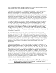 Expected emission reduction (relative to the respective
1990 certification levels for PM and NOX, respectively )
Variability of baseline conventional vehicle PM
measurement0
Variability of hybrid vehicle PM measurement
(assumed to be the same as for conventional vehicle)
Number of tests required to have 80% probability of
detecting expected PM emission reductiona
Variability for conventional vehicle NOX measurement
at 1990 levels0
Variability of hybrid vehicle NOX measurement
(assumed to be the same as for conventional vehicle)
Number of tests required to have 80% probability of
detecting expected NOx emission reduction11
5%
2%
2%
4
2%
2%
4
20%
2%
2%
2
2%
2%
2
50%
2%
3%
2
2%
7%
2
85%
2%
10%
2
2%
NAb
NAb
Computed under the assumption of normally distributed measurements having known variability.
Additional tests may be required if sample standard deviations obtained during testing are higher.
b NA = Not Available.
0 Variability of emission measurements from a chassis dynamometer is assumed to be the same as
historical data from an engine dynamometer laboratory running a baseline uncontrolled engine and
the same engine with add-on emission control technologies offering varying levels of control.
The fifth through the seventh rows (shaded) repeat the calculation for the NOX
measurement. No estimate of variability was available for the NOX measurement at an
85% reduction. Table xx shows that, for both PM and NOX, five tests are sufficient to
distinguish between zero and emissions reductions as low as 5%, based on the
assumption that the variability values in Table 2 represent the true variability values.
Two tests would be sufficient to detect the other emissions reductions, but three are
required by this protocol to provide a measured standard deviation.
15 Fuel Efficiency Calculation
FUEL CONSUMPTION - GRAVIMETRIC
At the conclusion of a test lap, the portable fuel tank is detached and weighed. The mass
of fuel consumed is the difference between the pre-test and post-test mass of the fuel tank
and fuel. The volume of fuel is calculated by dividing the mass consumed by the
measured density of the fuel:
V = m/p
Where V is the volume of fuel consumed during the test lap
M is the mass of fuel consumed during the test lap, and
P is the density of fuel as measured using ASTM method D-1298
54
image:
Expected emission reduction (relative to the respective
1990 certification levels for PM and NOX, respectively )
Variability of baseline conventional vehicle PM
measurement0
Variability of hybrid vehicle PM measurement
(assumed to be the same as for conventional vehicle)
Number of tests required to have 80% probability of
detecting expected PM emission reductiona
Variability for conventional vehicle NOX measurement
at 1990 levels0
Variability of hybrid vehicle NOX measurement
(assumed to be the same as for conventional vehicle)
Number of tests required to have 80% probability of
detecting expected NOx emission reduction11
5%
2%
2%
4
2%
2%
4
20%
2%
2%
2
2%
2%
2
50%
2%
3%
2
2%
7%
2
85%
2%
10%
2
2%
NAb
NAb
Computed under the assumption of normally distributed measurements having known variability.
Additional tests may be required if sample standard deviations obtained during testing are higher.
b NA = Not Available.
0 Variability of emission measurements from a chassis dynamometer is assumed to be the same as
historical data from an engine dynamometer laboratory running a baseline uncontrolled engine and
the same engine with add-on emission control technologies offering varying levels of control.
The fifth through the seventh rows (shaded) repeat the calculation for the NOX
measurement. No estimate of variability was available for the NOX measurement at an
85% reduction. Table xx shows that, for both PM and NOX, five tests are sufficient to
distinguish between zero and emissions reductions as low as 5%, based on the
assumption that the variability values in Table 2 represent the true variability values.
Two tests would be sufficient to detect the other emissions reductions, but three are
required by this protocol to provide a measured standard deviation.
15 Fuel Efficiency Calculation
FUEL CONSUMPTION - GRAVIMETRIC
At the conclusion of a test lap, the portable fuel tank is detached and weighed. The mass
of fuel consumed is the difference between the pre-test and post-test mass of the fuel tank
and fuel. The volume of fuel is calculated by dividing the mass consumed by the
measured density of the fuel:
V = m/p
Where V is the volume of fuel consumed during the test lap
M is the mass of fuel consumed during the test lap, and
P is the density of fuel as measured using ASTM method D-1298
54
image:
 For calculation of fuel efficiency from gravimetric data conversion factors are involved,
as the data are in mass units, but fuel efficiency is expressed in volumetric units (mi/gal
or k/L). SAE J1321, §A.3 describes the method of calculation and supplies the
conversion factors.
FUEL CONSUMPTION- CARBON-BALANCE
Fuel consumption can be measured by the carbon balance method, using data from the
exhaust gas analysis as described in SAE standard J1094a. This method calculates fuel
consumption from measured emissions of carbon-bearing gases. The calculations require
input of the emission rates (in grams/mile) of the total hydrocarbons (THC), carbon
monoxide (CO), and carbon dioxide (CO2).
These emissions can be measured using a conventional laboratory test cell or a portable
emissions monitoring system (PEMS). The laboratory test cell can only be used to
measure emissions of vehicles tested on a chassis dynamometer, whereas the PEMS can
be used to measure emissions of both dynamometer and track tests. The method of
calculation of fuel efficiency from emissions data shall be consistent with the procedure
described for automobiles in 40 CFR 600.113-93.
DISTANCE DRIVEN
Distance driven may be determined either by use of the vehicle odomometer, or by the
use of global positioning system (GPS) data. The use of GPS data would be applicable
only to track tests.
MASS-DISTANCE SPECIFIC METRICS
In some circumstances it might be appropriate to report the results in mass-distance
specific form, that is in a metric such as ton-miles per gallon. In most cases, this is not
necessary because the test payload is standardized, which means that the payload mass
remains a constant percentage of the maximum payload. However, if a truck is designed
to improve fuel efficiency through reduction of weight, it is possible that the maximum
payload will increase and thus the test payload, expressed as a percent of maximum
payload would also increase. In such a case, it would be informative to have the metric
reflect this increased efficiency. Reporting of a a mass-distance specific metric,
however, should be accompanied with all relevant information about paloads and percent
of maximum payload.
16 Reporting and Documentation
This section describes the procedures for reporting data, including what data must be
included and what format should be used.
16.1 Reports
The test report will contain the following topics:
1. Introduction;
55
image:
For calculation of fuel efficiency from gravimetric data conversion factors are involved,
as the data are in mass units, but fuel efficiency is expressed in volumetric units (mi/gal
or k/L). SAE J1321, §A.3 describes the method of calculation and supplies the
conversion factors.
FUEL CONSUMPTION- CARBON-BALANCE
Fuel consumption can be measured by the carbon balance method, using data from the
exhaust gas analysis as described in SAE standard J1094a. This method calculates fuel
consumption from measured emissions of carbon-bearing gases. The calculations require
input of the emission rates (in grams/mile) of the total hydrocarbons (THC), carbon
monoxide (CO), and carbon dioxide (CO2).
These emissions can be measured using a conventional laboratory test cell or a portable
emissions monitoring system (PEMS). The laboratory test cell can only be used to
measure emissions of vehicles tested on a chassis dynamometer, whereas the PEMS can
be used to measure emissions of both dynamometer and track tests. The method of
calculation of fuel efficiency from emissions data shall be consistent with the procedure
described for automobiles in 40 CFR 600.113-93.
DISTANCE DRIVEN
Distance driven may be determined either by use of the vehicle odomometer, or by the
use of global positioning system (GPS) data. The use of GPS data would be applicable
only to track tests.
MASS-DISTANCE SPECIFIC METRICS
In some circumstances it might be appropriate to report the results in mass-distance
specific form, that is in a metric such as ton-miles per gallon. In most cases, this is not
necessary because the test payload is standardized, which means that the payload mass
remains a constant percentage of the maximum payload. However, if a truck is designed
to improve fuel efficiency through reduction of weight, it is possible that the maximum
payload will increase and thus the test payload, expressed as a percent of maximum
payload would also increase. In such a case, it would be informative to have the metric
reflect this increased efficiency. Reporting of a a mass-distance specific metric,
however, should be accompanied with all relevant information about paloads and percent
of maximum payload.
16 Reporting and Documentation
This section describes the procedures for reporting data, including what data must be
included and what format should be used.
16.1 Reports
The test report will contain the following topics:
1. Introduction;
55
image:
 2. Description and identification of vehicle tested. Refer to SAE J2711 §6.2 and
SAE J1321 Type II Test Data Form 1;
3. Procedures and methods used in testing. Refer to SAE J1321 Type II Test Data
Forms 2-2 and 2-4;
4. Statement of operating range over which the test was conducted;
5. Discussion of results including:
a. Explanation and documentation of necessary deviations from the protocol,
and
b. Discussion of QA issues;
6. References; and
7. Appendices:
a. QA/QC activities and results,
b. Raw test data, and
c. Equipment calibration results.
16.2 Data and Metrics
The primary data collected is units of fuel consumption over units of time, distance, or
power. The mean of the test replicates and confidence limits shall be presented. The
carbon balance measurement method provides a methodology to convert carbon mass to
fuel consumed.
Metrics may include a fuel consumption rate per distance (gallons per mile) and/or per
time (gallons per hour) The fuel consumption per time metric accommodates vocational
trucks that consume fuel while conducting non-tractive mission work (operating a refuse
truck side arm and compacting trash; operating a utility aerial lift and supplying power to
the grid). This metric may be weighted into the fuel consumed per distance metric for
convenience and ease of comparison, using an appropriate weighting for that vehicle
application, which would be described in the "drive cycle." For over-the-road freight
truck applications like highway line haul and regional haul, a gallon per ton-mile metric,
as decribed in the previous section, "mass-distance specific metrics," may be most
reasonable, since the main function of these vehicles is to carry tonnage. This metric
could be readily calculated using the test results of fuel consumption, distance, and
payload factors in the drive cycle.
If a testing organization wishes to collect emissions data other than carbon, this data shall
be reported as emission rates in grams/kilowatt-hour (g/kW-h) [grams/brake horsepower-
hour (g/bhp-hr)], grams/mile (g/mi) [grams/kilometer (g/km)] or as grams per cycle,
depending on the test method (track or chassis) and the user's decision as to which is the
most appropriate.
16.3 Quality Assurance and Control
Quality assurance and quality control procedures are used to ensure the accuracy and
precision of test results. Accuracy of fuel consumption measurements is primarily
dependent on the accuracy of the following measurements:
56
image:
2. Description and identification of vehicle tested. Refer to SAE J2711 §6.2 and
SAE J1321 Type II Test Data Form 1;
3. Procedures and methods used in testing. Refer to SAE J1321 Type II Test Data
Forms 2-2 and 2-4;
4. Statement of operating range over which the test was conducted;
5. Discussion of results including:
a. Explanation and documentation of necessary deviations from the protocol,
and
b. Discussion of QA issues;
6. References; and
7. Appendices:
a. QA/QC activities and results,
b. Raw test data, and
c. Equipment calibration results.
16.2 Data and Metrics
The primary data collected is units of fuel consumption over units of time, distance, or
power. The mean of the test replicates and confidence limits shall be presented. The
carbon balance measurement method provides a methodology to convert carbon mass to
fuel consumed.
Metrics may include a fuel consumption rate per distance (gallons per mile) and/or per
time (gallons per hour) The fuel consumption per time metric accommodates vocational
trucks that consume fuel while conducting non-tractive mission work (operating a refuse
truck side arm and compacting trash; operating a utility aerial lift and supplying power to
the grid). This metric may be weighted into the fuel consumed per distance metric for
convenience and ease of comparison, using an appropriate weighting for that vehicle
application, which would be described in the "drive cycle." For over-the-road freight
truck applications like highway line haul and regional haul, a gallon per ton-mile metric,
as decribed in the previous section, "mass-distance specific metrics," may be most
reasonable, since the main function of these vehicles is to carry tonnage. This metric
could be readily calculated using the test results of fuel consumption, distance, and
payload factors in the drive cycle.
If a testing organization wishes to collect emissions data other than carbon, this data shall
be reported as emission rates in grams/kilowatt-hour (g/kW-h) [grams/brake horsepower-
hour (g/bhp-hr)], grams/mile (g/mi) [grams/kilometer (g/km)] or as grams per cycle,
depending on the test method (track or chassis) and the user's decision as to which is the
most appropriate.
16.3 Quality Assurance and Control
Quality assurance and quality control procedures are used to ensure the accuracy and
precision of test results. Accuracy of fuel consumption measurements is primarily
dependent on the accuracy of the following measurements:
56
image:
 • For fuel consumption measured by carbon-balance method:
o Accuracy of gas analyses for CO2, CO and HC
o Accuracy of exhaust flow determination
o Accuracy of fuel carbon and density
• For fuel consumption measured by gravimetric method:
o Accuracy of scales used to weigh fuel
o Accuracy of measurements of fuel density and temperature correction
• For tests conducted on a dynamometer
o Accuracy of dynamometer force simulation
o Accuracy of estimates of road load and aerodynamic drag
o Accuracy of speed and distance measurements
• For tests conducted on a test track
o Accuracy of speed measurements
o Accuracy of distance measurements
Accuracy of these measurements is primarily documented by the use of calibration of the
instruments and other measuring devices against known standards. The specific
calibration details for the measurements needed are given in the appropriate test
descriptions, including SAE and ASTM test method documentation of the relevant parts
of the Code of Federal Regulations.
In addition to such documentation, the accuracy of the fuel efficiency metric ccan be
directly tested by comparison of standardized reference trucks, for which the fuel
efficiency has been tested multiple times by multiple laboratories.
The short-term precision of a fuel efficiency test method is estimated by use of replicate
tests. The acceptable level of precision is determined by the final user of the test results,
and sufficient replicate measurements should be taken to ensure that the acceptable level
of precision can be documented.
Quality assurance activities should be documented by the following:
• Standard Operating Procedures to ensure that test procedures are done properly
• Records of instrument calibrations
• Records of replicate tests and calculations of precision estimates
• Records of calculations of fuel efficiency
• Daily test log that documents all testing activities, including anomalous behavior
and events that could affect test results.
16.4 Assessment
Each testing organization should conduct an internal assessment of its quality and
technical systems and should allow external assessments of these systems by QA
personnel. After an assessment, the testing organization will be responsible for
developing and implementing corrective actions in response to the assessment's findings.
57
image:
• For fuel consumption measured by carbon-balance method:
o Accuracy of gas analyses for CO2, CO and HC
o Accuracy of exhaust flow determination
o Accuracy of fuel carbon and density
• For fuel consumption measured by gravimetric method:
o Accuracy of scales used to weigh fuel
o Accuracy of measurements of fuel density and temperature correction
• For tests conducted on a dynamometer
o Accuracy of dynamometer force simulation
o Accuracy of estimates of road load and aerodynamic drag
o Accuracy of speed and distance measurements
• For tests conducted on a test track
o Accuracy of speed measurements
o Accuracy of distance measurements
Accuracy of these measurements is primarily documented by the use of calibration of the
instruments and other measuring devices against known standards. The specific
calibration details for the measurements needed are given in the appropriate test
descriptions, including SAE and ASTM test method documentation of the relevant parts
of the Code of Federal Regulations.
In addition to such documentation, the accuracy of the fuel efficiency metric ccan be
directly tested by comparison of standardized reference trucks, for which the fuel
efficiency has been tested multiple times by multiple laboratories.
The short-term precision of a fuel efficiency test method is estimated by use of replicate
tests. The acceptable level of precision is determined by the final user of the test results,
and sufficient replicate measurements should be taken to ensure that the acceptable level
of precision can be documented.
Quality assurance activities should be documented by the following:
• Standard Operating Procedures to ensure that test procedures are done properly
• Records of instrument calibrations
• Records of replicate tests and calculations of precision estimates
• Records of calculations of fuel efficiency
• Daily test log that documents all testing activities, including anomalous behavior
and events that could affect test results.
16.4 Assessment
Each testing organization should conduct an internal assessment of its quality and
technical systems and should allow external assessments of these systems by QA
personnel. After an assessment, the testing organization will be responsible for
developing and implementing corrective actions in response to the assessment's findings.
57
image:
 As appropriate, an organization with oversight responsibilities may conduct assessments
to determine the testing organization's compliance with its test/QA plan. Examples of
assessments are described in EPA's ETV QMP.30 It is highly recommended that
assessments be conducted with a rigor comparable to those described in EPA's Guidance
on Technical Audits and Related Assessment for Environmental Data Operations 31 and
Guidance on Assessing Quality Systems32
17 Appendices
58
image:
As appropriate, an organization with oversight responsibilities may conduct assessments
to determine the testing organization's compliance with its test/QA plan. Examples of
assessments are described in EPA's ETV QMP.30 It is highly recommended that
assessments be conducted with a rigor comparable to those described in EPA's Guidance
on Technical Audits and Related Assessment for Environmental Data Operations 31 and
Guidance on Assessing Quality Systems32
17 Appendices
58
image:
 17.1 Appendix A
Abbreviations and Acronyms
ACEEE American Council for an Energy Efficient Economy
bhp brake horsepower
Btu British thermal unit
CARB California Air Resources Board
CBI confidential business information
cfm cubic feet per minute
CFR Code of Federal Regulations
CO carbon monoxide
CO2 carbon dioxide
cu. yd. cubic yard
DQO data quality objective
EPA Environmental Protection Agency
EPAct 2005 Energy Policy Act of 2005
ETV Environmental Technology Verification Program
ft feet
FTA Federal Transit Administration
FTP federal test procedure
gal gallon
g/mi grams per mile
g/bhp-hr grams per brake horsepower-hour
g/kWh grams per kilowatt-hour
GVWR gross vehicle weight rating
WC ratio Hybrid Vehicle Fuel Used/Comparable Baseline Vehicle Fuel Used
HAP hazardous air pollutant
HDHV heavy duty hybrid vehicle
hp horsepower
HVAC heating, ventilation, and air conditioning
in inches
IRS Internal Revenue Service
km kilometer
L liter
Ib pound
mph miles per hour
NEC net energy change
NO nitric oxide
NO2 nitrogen dioxide
NOx nitrogen oxides
NREL National Renewable Energy Laboratory
NYCT New York City Transit
OBD on-board diagnostics
ORD Office of Research and Development
OTAQ Office of Transportation and Air Quality
59
image:
17.1 Appendix A
Abbreviations and Acronyms
ACEEE American Council for an Energy Efficient Economy
bhp brake horsepower
Btu British thermal unit
CARB California Air Resources Board
CBI confidential business information
cfm cubic feet per minute
CFR Code of Federal Regulations
CO carbon monoxide
CO2 carbon dioxide
cu. yd. cubic yard
DQO data quality objective
EPA Environmental Protection Agency
EPAct 2005 Energy Policy Act of 2005
ETV Environmental Technology Verification Program
ft feet
FTA Federal Transit Administration
FTP federal test procedure
gal gallon
g/mi grams per mile
g/bhp-hr grams per brake horsepower-hour
g/kWh grams per kilowatt-hour
GVWR gross vehicle weight rating
WC ratio Hybrid Vehicle Fuel Used/Comparable Baseline Vehicle Fuel Used
HAP hazardous air pollutant
HDHV heavy duty hybrid vehicle
hp horsepower
HVAC heating, ventilation, and air conditioning
in inches
IRS Internal Revenue Service
km kilometer
L liter
Ib pound
mph miles per hour
NEC net energy change
NO nitric oxide
NO2 nitrogen dioxide
NOx nitrogen oxides
NREL National Renewable Energy Laboratory
NYCT New York City Transit
OBD on-board diagnostics
ORD Office of Research and Development
OTAQ Office of Transportation and Air Quality
59
image:
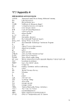 PEMS portable emissions monitoring system
PM particulate matter
[Reserved]
60
image:
PEMS portable emissions monitoring system
PM particulate matter
[Reserved]
60
image:
 17.2-17.8 Appendices B - H
[Reserved]
61
image:
17.2-17.8 Appendices B - H
[Reserved]
61
image:
 17.9 Appendix I
Statistics - Test Track Testing
Example Sample Size Calculation for Emission Reduction
This appendix presents sample calculations for determining the minimum number of tests
required to detect a significant emissions or fuel consumption reduction. The calculation
is based on:
1) The emissions variability is taken to be known for the population of measurements;
2) A known baseline conventional vehicle mean emission;
3) A mean hybrid vehicle emission (the product of the conventional vehicle emission
and the expected emissions reduction); and
4) One part of the equation is based on the assumption of known standard deviations
and the normal distribution. However, since the actual testing procedure is based
on sample standard deviations and t-statistics, a correction factor is added to the
sample-size equation to account for the extra variation in the t-distribution relative
to that of the normal distribution.
The criterion being used is that the minimum number of tests required for use of this
protocol is the number of tests required to have an 80% probability of detecting the
specified emission reduction at the 95% confidence level. The basic equation being used
for the calculation is:
where:
n = sample size in each group, rounded up to the next integer;
za = normal distribution value corresponding to upper-tail probability of a ;
and
zp = normal distribution value corresponding to upper-tail probability of ft.
I -a = confidence coefficient on comparison of means (0.95 minimum);
I-/? = probability of detection of reduction/increase (0.80 minimum);
cr^ = squared standard deviation of conventional vehicle emission data,
expressed as a percent of the conventional vehicle emission value;
<J2H = squared standard deviation of hybrid vehicle emission data, expressed as a
percent of the conventional vehicle emission value;
6 = difference between conventional and hybrid vehicle emissions mean,
expressed as a percent of the conventional vehicle emission value.
62
image:
17.9 Appendix I
Statistics - Test Track Testing
Example Sample Size Calculation for Emission Reduction
This appendix presents sample calculations for determining the minimum number of tests
required to detect a significant emissions or fuel consumption reduction. The calculation
is based on:
1) The emissions variability is taken to be known for the population of measurements;
2) A known baseline conventional vehicle mean emission;
3) A mean hybrid vehicle emission (the product of the conventional vehicle emission
and the expected emissions reduction); and
4) One part of the equation is based on the assumption of known standard deviations
and the normal distribution. However, since the actual testing procedure is based
on sample standard deviations and t-statistics, a correction factor is added to the
sample-size equation to account for the extra variation in the t-distribution relative
to that of the normal distribution.
The criterion being used is that the minimum number of tests required for use of this
protocol is the number of tests required to have an 80% probability of detecting the
specified emission reduction at the 95% confidence level. The basic equation being used
for the calculation is:
where:
n = sample size in each group, rounded up to the next integer;
za = normal distribution value corresponding to upper-tail probability of a ;
and
zp = normal distribution value corresponding to upper-tail probability of ft.
I -a = confidence coefficient on comparison of means (0.95 minimum);
I-/? = probability of detection of reduction/increase (0.80 minimum);
cr^ = squared standard deviation of conventional vehicle emission data,
expressed as a percent of the conventional vehicle emission value;
<J2H = squared standard deviation of hybrid vehicle emission data, expressed as a
percent of the conventional vehicle emission value;
6 = difference between conventional and hybrid vehicle emissions mean,
expressed as a percent of the conventional vehicle emission value.
62
image:
 Note that o2c , a2H , and S are expressed as percentages of the conventional vehicle
emission. This transformation was used to simplify the equation and allow its use for
Table 1 in Section 5.3.1. For Table 1, the baseline conventional vehicle mean emission
value was 12.495 grams/mile, taken from the suburban drive cycle of the Kenworth data.1
The parameter V is tabulated under different names in statistics reference texts. It is the
V value corresponding to 'the tail area of the unit normal distribution' in Box, Hunter,
and Hunter (1978). In the Standard Mathematical Tables (CRC, 1968), V is known as
'x', and the tail area is labeled ' 1 - F(x)\ where F(x) is the cumulative distribution
function of a standardized normal random variable. To obtain the value of V from the
statistical tables, a (or /?) is the probability (ranging from 0.5000 to 0.0000) in the body of
the table, and V is read (or interpolated) from the appropriate column and/or row,
ranging from 0.00 to 4.00 over that range. The value V can be calculated within an
EXCEL® or QUATTRO PRO® spreadsheet as the absolute value of the function
returning the inverse of the standard normal cumulative distribution,
NORMSINV(probability), by setting probability equal to a or/?, as appropriate. A
derivation of the correction factor, z2a/2, is available in Appendix A of the EPA G-4
guidance document (Guidance on the Data Quality Objectives Process (EPA/600/R-
96/055)).
Table C-l gives a step-by-step calculation example drawn from Table 1 for an 80%
probability (fi = 0.20) of detecting a 5% and a 50% emission reduction at the 95%
confidence level (a = 0.05).
_Proper citation is needed, here, for the Kenworth truck testing dataset.
63
image:
Note that o2c , a2H , and S are expressed as percentages of the conventional vehicle
emission. This transformation was used to simplify the equation and allow its use for
Table 1 in Section 5.3.1. For Table 1, the baseline conventional vehicle mean emission
value was 12.495 grams/mile, taken from the suburban drive cycle of the Kenworth data.1
The parameter V is tabulated under different names in statistics reference texts. It is the
V value corresponding to 'the tail area of the unit normal distribution' in Box, Hunter,
and Hunter (1978). In the Standard Mathematical Tables (CRC, 1968), V is known as
'x', and the tail area is labeled ' 1 - F(x)\ where F(x) is the cumulative distribution
function of a standardized normal random variable. To obtain the value of V from the
statistical tables, a (or /?) is the probability (ranging from 0.5000 to 0.0000) in the body of
the table, and V is read (or interpolated) from the appropriate column and/or row,
ranging from 0.00 to 4.00 over that range. The value V can be calculated within an
EXCEL® or QUATTRO PRO® spreadsheet as the absolute value of the function
returning the inverse of the standard normal cumulative distribution,
NORMSINV(probability), by setting probability equal to a or/?, as appropriate. A
derivation of the correction factor, z2a/2, is available in Appendix A of the EPA G-4
guidance document (Guidance on the Data Quality Objectives Process (EPA/600/R-
96/055)).
Table C-l gives a step-by-step calculation example drawn from Table 1 for an 80%
probability (fi = 0.20) of detecting a 5% and a 50% emission reduction at the 95%
confidence level (a = 0.05).
_Proper citation is needed, here, for the Kenworth truck testing dataset.
63
image:
 Table C-l. Example calculation of minimum number of replicate test track tests
required to achieve an 80% probability of detecting emission reductions
at a confidence level of 95%.
Emission reduction relative to conventional vehicle emission, S, %
Known measurement variability for conventional vehicle, ac , %
Known measurement variability for hybrid vehicle, aH , %
a
Za
ft
Zfi
\<j2H+(j2c(l-5llW}2^\/52
(za+zp)2[a2H+a2(l-S/WO)2]/S2
4/2
(Za+Zp)2[a2H+a2(l-S/WO)2]/S2+z2a/2
Number of tests required , n
Table 1,
Col.l
5
2.58
2.58
0.05
1.645
0.20
0.842
0.514
3.18
1.35
4.53
5
Table 1,
Col. 3
50
2.58
2.58
0.05
1.645
0.20
0.842
0.003
0.02
1.35
1.37
2a
Note: The minimum number of tests is three. If'«' is less than three, '«' equals three.
Example Sample Size Calculation for Fuel efficiency Improvement
This appendix presents example calculations to illustrate calculation of the minimum
number of tests required to detect a significant fuel efficiency improvement.
The calculation is based on:
1) The fuel efficiency variability is taken to be known for the population of
measurements;
2) A known baseline conventional vehicle mean fuel efficiency;
3) A mean hybrid vehicle fuel efficiency; and
4) One part of the equation is based on the assumption of known standard deviations
and the normal distribution. However, since the actual testing procedure is based
64
image:
Table C-l. Example calculation of minimum number of replicate test track tests
required to achieve an 80% probability of detecting emission reductions
at a confidence level of 95%.
Emission reduction relative to conventional vehicle emission, S, %
Known measurement variability for conventional vehicle, ac , %
Known measurement variability for hybrid vehicle, aH , %
a
Za
ft
Zfi
\<j2H+(j2c(l-5llW}2^\/52
(za+zp)2[a2H+a2(l-S/WO)2]/S2
4/2
(Za+Zp)2[a2H+a2(l-S/WO)2]/S2+z2a/2
Number of tests required , n
Table 1,
Col.l
5
2.58
2.58
0.05
1.645
0.20
0.842
0.514
3.18
1.35
4.53
5
Table 1,
Col. 3
50
2.58
2.58
0.05
1.645
0.20
0.842
0.003
0.02
1.35
1.37
2a
Note: The minimum number of tests is three. If'«' is less than three, '«' equals three.
Example Sample Size Calculation for Fuel efficiency Improvement
This appendix presents example calculations to illustrate calculation of the minimum
number of tests required to detect a significant fuel efficiency improvement.
The calculation is based on:
1) The fuel efficiency variability is taken to be known for the population of
measurements;
2) A known baseline conventional vehicle mean fuel efficiency;
3) A mean hybrid vehicle fuel efficiency; and
4) One part of the equation is based on the assumption of known standard deviations
and the normal distribution. However, since the actual testing procedure is based
64
image:
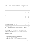 on sample standard deviations and t-statistics, a correction factor is added to the
sample-size equation to account for the extra variation in the t-distribution relative
to that of the normal distribution.
The criterion being used is that the minimum number of tests required for use of this
protocol is the number of tests required to have an 80% probability of detecting the
specified fuel efficiency increase at the 95% confidence level. The basic equation being
used for the calculation is:
where:
n = sample size in each group, rounded up to the next integer;
za = normal distribution value corresponding to upper-tail probability of a ;
and
z p = normal distribution value corresponding to upper-tail probability of ft.
I - a = confidence coefficient on comparison of means (0.95 minimum);
I-/? = probability of detection of reduction/increase (0.80 minimum);
cr^ = squared standard deviation of conventional vehicle fuel efficiency data,
expressed as a percent of the conventional vehicle fuel efficiency value;
a2H = squared standard deviation of hybrid vehicle fuel efficiency data,
expressed as a percent of the conventional vehicle fuel efficiency value;
S = difference between conventional and hybrid vehicle fuel efficiency mean,
expressed as a percent of the conventional vehicle fuel efficiency value.
Note that a2C , a2H , and 6 are expressed as percentages of the conventional vehicle fuel
efficiency. This transformation was used to simplify the equation and allow its use for
Table 1. The parameter V is tabulated under different names in statistics reference texts.
It is the V value corresponding to 'the tail area of the unit normal distribution' in Box,
Hunter, and Hunter (1978). In the Standard Mathematical Tables (CRC, 1968), V is
known as 'x', and the tail area is labeled ' 1 - F(x)', where F(x) is the cumulative
distribution function of a standardized normal random variable. To obtain the value of
V from the statistical tables, a (or/?) is the probability (ranging from 0.5000 to 0.0000)
in the body of the table, and V is read (or interpolated) from the appropriate column
and/or row, ranging from 0.00 to 4.00 over that range. The value V can be calculated
within an EXCEL® or QUATTRO PRO® spreadsheet as the absolute value of the
function returning the inverse of the standard normal cumulative distribution,
NORMSINV(probability), by setting probability equal to a or/?, as appropriate. A
derivation of the correction factor, z^/2, is available in Appendix A of the EPA G-4
65
image:
on sample standard deviations and t-statistics, a correction factor is added to the
sample-size equation to account for the extra variation in the t-distribution relative
to that of the normal distribution.
The criterion being used is that the minimum number of tests required for use of this
protocol is the number of tests required to have an 80% probability of detecting the
specified fuel efficiency increase at the 95% confidence level. The basic equation being
used for the calculation is:
where:
n = sample size in each group, rounded up to the next integer;
za = normal distribution value corresponding to upper-tail probability of a ;
and
z p = normal distribution value corresponding to upper-tail probability of ft.
I - a = confidence coefficient on comparison of means (0.95 minimum);
I-/? = probability of detection of reduction/increase (0.80 minimum);
cr^ = squared standard deviation of conventional vehicle fuel efficiency data,
expressed as a percent of the conventional vehicle fuel efficiency value;
a2H = squared standard deviation of hybrid vehicle fuel efficiency data,
expressed as a percent of the conventional vehicle fuel efficiency value;
S = difference between conventional and hybrid vehicle fuel efficiency mean,
expressed as a percent of the conventional vehicle fuel efficiency value.
Note that a2C , a2H , and 6 are expressed as percentages of the conventional vehicle fuel
efficiency. This transformation was used to simplify the equation and allow its use for
Table 1. The parameter V is tabulated under different names in statistics reference texts.
It is the V value corresponding to 'the tail area of the unit normal distribution' in Box,
Hunter, and Hunter (1978). In the Standard Mathematical Tables (CRC, 1968), V is
known as 'x', and the tail area is labeled ' 1 - F(x)', where F(x) is the cumulative
distribution function of a standardized normal random variable. To obtain the value of
V from the statistical tables, a (or/?) is the probability (ranging from 0.5000 to 0.0000)
in the body of the table, and V is read (or interpolated) from the appropriate column
and/or row, ranging from 0.00 to 4.00 over that range. The value V can be calculated
within an EXCEL® or QUATTRO PRO® spreadsheet as the absolute value of the
function returning the inverse of the standard normal cumulative distribution,
NORMSINV(probability), by setting probability equal to a or/?, as appropriate. A
derivation of the correction factor, z^/2, is available in Appendix A of the EPA G-4
65
image:
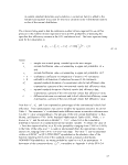 guidance document {Guidance on the Data Quality Objectives Process (EPA/600/R-
96/055)).
Table C-2 gives a step-by-step calculation example drawn from Table 1 for an 80%
probability (ft = 0.20) of detecting a 5% and a 50% fuel efficiency increase at the 95%
confidence level (a = 0.05).
Table C-2. Example calculation of minimum number of tests.
Fuel efficiency increase relative to conventional vehicle fuel efficiency,
S,%
Known measurement variability for conventional vehicle, ac , %
Known measurement variability for hybrid vehicle, <JH , %
a
Za
ft
Zfi
Tc4+crc(l + £/100)2l/£2
(za+zp)2[al+al(\ + 6l\W)*]/?
z2Jl
(za+Zp)2[vl+rt(l + 5HW}2]/5^+zll2
Number of tests required , n
Table 1,
Col.l
5
2.46
2.46
0.05
1.645
0.20
0.842
0.509
3.15
1.35
4.50
5
Table 1,
Col. 3
50
2.46
2.46
0.05
1.645
0.20
0.842
0.003
0.02
1.35
1.37
2a
Note:
The minimum number of tests is three. If '«' is less than three, '«' equals three.
Statistics - Chassis Dynamometer Testing
The calculations for the minimum number of tests required to detect a significant
emissions reduction or fuel efficiency increase are identical to those presented in the
preceding section.
Based on the calculations presented in the preceding section, Table D-l gives a step-by-
step calculation example drawn from Table 2 of Section 5.3.2 for an 80% probability (ft =
66
image:
guidance document {Guidance on the Data Quality Objectives Process (EPA/600/R-
96/055)).
Table C-2 gives a step-by-step calculation example drawn from Table 1 for an 80%
probability (ft = 0.20) of detecting a 5% and a 50% fuel efficiency increase at the 95%
confidence level (a = 0.05).
Table C-2. Example calculation of minimum number of tests.
Fuel efficiency increase relative to conventional vehicle fuel efficiency,
S,%
Known measurement variability for conventional vehicle, ac , %
Known measurement variability for hybrid vehicle, <JH , %
a
Za
ft
Zfi
Tc4+crc(l + £/100)2l/£2
(za+zp)2[al+al(\ + 6l\W)*]/?
z2Jl
(za+Zp)2[vl+rt(l + 5HW}2]/5^+zll2
Number of tests required , n
Table 1,
Col.l
5
2.46
2.46
0.05
1.645
0.20
0.842
0.509
3.15
1.35
4.50
5
Table 1,
Col. 3
50
2.46
2.46
0.05
1.645
0.20
0.842
0.003
0.02
1.35
1.37
2a
Note:
The minimum number of tests is three. If '«' is less than three, '«' equals three.
Statistics - Chassis Dynamometer Testing
The calculations for the minimum number of tests required to detect a significant
emissions reduction or fuel efficiency increase are identical to those presented in the
preceding section.
Based on the calculations presented in the preceding section, Table D-l gives a step-by-
step calculation example drawn from Table 2 of Section 5.3.2 for an 80% probability (ft =
66
image:
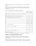 0.20) of detecting a 5% and a 50% emission reduction at the 95% confidence level (a =
0.05).
Table D-l. Example calculation of minimum number of replicate chassis
dynamometer tests to achieve an 80% probability of detecting emissions
reductions at a confidence limit of 95%.
Emission reduction relative to conventional vehicle emission, S, %
Known measurement variability for conventional vehicle, ac , %
Known measurement variability for hybrid vehicle, <JH , %
a
ZCL
ft
ZP
[<4+^(i-£/ioo)2]/£2
(za+Zp)2[al+a2c(\-5l\W}2]/52
t/2
(za+zp)2[a2H+a2(l-S/WO)2]/S2+z2a/2
Number of tests requireda, n
Table 2,
Col.l
5
2
2
0.05
1.645
0.20
0.842
0.304
1.88
1.35
3.23
4
Table 2,
Col. 3
50
2
3
0.05
1.645
0.20
0.842
0.004
0.02
1.35
1.38
2a
Note:
The minimum number of tests is three. If'«' is less than three, '«' equals three.
References
CRC. Standard Mathematical Tables, 16th Ed. S. Shelby, Ed. The Chemical Rubber
Company, Cleveland, OH. 1968.
Box, G. E. P., W. G. Hunter, and J. S. Hunter. Statistics for Experimenters. John Wiley
& Sons, New York, NY. 1978.
EXCEL®. Microsoft Corporation, Redland, WA. 2001.
QUATTRO PRO®. Corel Corporation, Ottawa, Ontario, CANADA. 2001.
67
image:
0.20) of detecting a 5% and a 50% emission reduction at the 95% confidence level (a =
0.05).
Table D-l. Example calculation of minimum number of replicate chassis
dynamometer tests to achieve an 80% probability of detecting emissions
reductions at a confidence limit of 95%.
Emission reduction relative to conventional vehicle emission, S, %
Known measurement variability for conventional vehicle, ac , %
Known measurement variability for hybrid vehicle, <JH , %
a
ZCL
ft
ZP
[<4+^(i-£/ioo)2]/£2
(za+Zp)2[al+a2c(\-5l\W}2]/52
t/2
(za+zp)2[a2H+a2(l-S/WO)2]/S2+z2a/2
Number of tests requireda, n
Table 2,
Col.l
5
2
2
0.05
1.645
0.20
0.842
0.304
1.88
1.35
3.23
4
Table 2,
Col. 3
50
2
3
0.05
1.645
0.20
0.842
0.004
0.02
1.35
1.38
2a
Note:
The minimum number of tests is three. If'«' is less than three, '«' equals three.
References
CRC. Standard Mathematical Tables, 16th Ed. S. Shelby, Ed. The Chemical Rubber
Company, Cleveland, OH. 1968.
Box, G. E. P., W. G. Hunter, and J. S. Hunter. Statistics for Experimenters. John Wiley
& Sons, New York, NY. 1978.
EXCEL®. Microsoft Corporation, Redland, WA. 2001.
QUATTRO PRO®. Corel Corporation, Ottawa, Ontario, CANADA. 2001.
67
image:
 17.10 Appendix J
Calculations to Compare the Hybrid Version of a Heavy Duty
Vehicle to the Non-Hybrid Version
Comparative testing of a hybrid vehicle to its non-hybrid "twin," whether the testing is
conducted on a test track or on a chassis dynamometer, involves multiple tests of a
baseline conventional vehicle and multiple tests of a hybrid vehicle. This section
describes the data analysis procedure that will be used to calculate the emission
reductions and increase in fuel efficiency from these data.
This calculation assumes that the same test method (test track or chassis dynamometer) is
used for all the testing.
Procedure for Calculating Emission Reduction
Let EC and EH refer to the emission rates of a single pollutant for conventional and hybrid
vehicles, respectively. Once the E values for the tests are available, the corresponding
sample means (Ec and EH) and standard deviations (sc and SH) are computed using
Equations 2 and 3.
"C »H
IX, _ IX,
Ec = — and EH = —
nc
sc = JS fe - Ec ) (nc ~ 1) and SH = £ (EHJ - EH ) (nH -1)
V i / V i / (3)
where:
Ec = mean emission rate for the conventional vehicle for a single pollutant,
EH = mean emission rate for the hybrid vehicle for a single pollutant,
Ecjt = emission rate for a single conventional ith test for a single pollutant,
EH* = emission rate for a single hybrid ith test for a single pollutant,
nc and nH = number of conventional and hybrid tests, and
sc and SH = standard deviations of conventional and hybrid tests.
The raw emission reduction for each pollutant, ERRAW-, is then computed as the difference
between the mean emission rates for the conventional and hybrid cases, divided by the
conventional case mean emission rate, as shown in Equation 4.
ERRAW = (EC - EH }/EC . .
68
image:
17.10 Appendix J
Calculations to Compare the Hybrid Version of a Heavy Duty
Vehicle to the Non-Hybrid Version
Comparative testing of a hybrid vehicle to its non-hybrid "twin," whether the testing is
conducted on a test track or on a chassis dynamometer, involves multiple tests of a
baseline conventional vehicle and multiple tests of a hybrid vehicle. This section
describes the data analysis procedure that will be used to calculate the emission
reductions and increase in fuel efficiency from these data.
This calculation assumes that the same test method (test track or chassis dynamometer) is
used for all the testing.
Procedure for Calculating Emission Reduction
Let EC and EH refer to the emission rates of a single pollutant for conventional and hybrid
vehicles, respectively. Once the E values for the tests are available, the corresponding
sample means (Ec and EH) and standard deviations (sc and SH) are computed using
Equations 2 and 3.
"C »H
IX, _ IX,
Ec = — and EH = —
nc
sc = JS fe - Ec ) (nc ~ 1) and SH = £ (EHJ - EH ) (nH -1)
V i / V i / (3)
where:
Ec = mean emission rate for the conventional vehicle for a single pollutant,
EH = mean emission rate for the hybrid vehicle for a single pollutant,
Ecjt = emission rate for a single conventional ith test for a single pollutant,
EH* = emission rate for a single hybrid ith test for a single pollutant,
nc and nH = number of conventional and hybrid tests, and
sc and SH = standard deviations of conventional and hybrid tests.
The raw emission reduction for each pollutant, ERRAW-, is then computed as the difference
between the mean emission rates for the conventional and hybrid cases, divided by the
conventional case mean emission rate, as shown in Equation 4.
ERRAW = (EC - EH }/EC . .
68
image:
 The upper and lower bounds of the approximate confidence interval (CT) around
are computed using Equations 5a and 5b.
CI (upper bound) = ERRAW+\\ ta/2 • p- + (l-ERRAW)2±- IE,
V I'JLT l'f^ I /
(5a)
CI (lower bound) = ERRAW -
/ C i V
I H , /I 777? \2 AC
|- + (l-^_) -
In the equations above, to/2 is the (1 - a/2) percentile of the t-distribution, with degrees of
freedom, u, given by Equation 6 (rounded down)2, and a = 1 - (confidence level /100%).
However, since the testing procedure is interested only in unidirect!onal positive
reductions, one-tailed tests will be conducted. Consequently, only the lower bound of the
confidence interval will be of interest, and ta will replace ta/2 in Equation 5b. Thus, in
tables giving distributions oft for two-tailed tests, use 2a to obtain the critical value. For
example, if the confidence level is 95%, then a = 0.05; if in addition, v = 5, then ta =
2.015.
^S2H/nH+(l-ERRAir)2s2c/nc
u =
The fractional values of emission reduction and the confidence intervals are converted to
percentages by multiplying by 100 percent.
5.2.2.2 Procedure for Calculating Fuel efficiency Improvement
Let FC and FH refer to the fuel efficiency rates in miles per gallon (MPG) for baseline
conventional and hybrid vehicles, respectively. Once the F values for the tests are
available, the corresponding sample means (Fc and FH ) and standard deviations (sc and
SH) are computed using Equations 2 and 3, except that FC and FH values are used instead
of EC and EH values in the formulas.
The raw fuel efficiency increase, F!RAW, is then computed as the difference between the
mean fuel efficiency rates for the hybrid and conventional cases, divided by the baseline
conventional case mean fuel efficiency rate, as shown in Equation 7.
FI =
1 1RAW
-F
l
(5b)
(6)
(7)
' The value of o rounded down from Equation 9 can generally be approximated as nc + nH - 3.
69
image:
The upper and lower bounds of the approximate confidence interval (CT) around
are computed using Equations 5a and 5b.
CI (upper bound) = ERRAW+\\ ta/2 • p- + (l-ERRAW)2±- IE,
V I'JLT l'f^ I /
(5a)
CI (lower bound) = ERRAW -
/ C i V
I H , /I 777? \2 AC
|- + (l-^_) -
In the equations above, to/2 is the (1 - a/2) percentile of the t-distribution, with degrees of
freedom, u, given by Equation 6 (rounded down)2, and a = 1 - (confidence level /100%).
However, since the testing procedure is interested only in unidirect!onal positive
reductions, one-tailed tests will be conducted. Consequently, only the lower bound of the
confidence interval will be of interest, and ta will replace ta/2 in Equation 5b. Thus, in
tables giving distributions oft for two-tailed tests, use 2a to obtain the critical value. For
example, if the confidence level is 95%, then a = 0.05; if in addition, v = 5, then ta =
2.015.
^S2H/nH+(l-ERRAir)2s2c/nc
u =
The fractional values of emission reduction and the confidence intervals are converted to
percentages by multiplying by 100 percent.
5.2.2.2 Procedure for Calculating Fuel efficiency Improvement
Let FC and FH refer to the fuel efficiency rates in miles per gallon (MPG) for baseline
conventional and hybrid vehicles, respectively. Once the F values for the tests are
available, the corresponding sample means (Fc and FH ) and standard deviations (sc and
SH) are computed using Equations 2 and 3, except that FC and FH values are used instead
of EC and EH values in the formulas.
The raw fuel efficiency increase, F!RAW, is then computed as the difference between the
mean fuel efficiency rates for the hybrid and conventional cases, divided by the baseline
conventional case mean fuel efficiency rate, as shown in Equation 7.
FI =
1 1RAW
-F
l
(5b)
(6)
(7)
' The value of o rounded down from Equation 9 can generally be approximated as nc + nH - 3.
69
image:
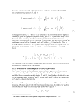 The upper and lower bounds of the approximate confidence interval (CI) around F!RAW
are computed using Equations 8a and 8b.
CI (upper bound) = FIRAW +\ ta!2
(8a)
CI (lower bound) = FIRAW -
In the equations above, to/2 is the (1 - a/2) percentile of the t-distribution, with degrees of
freedom, u, given by Equation 9 (rounded down)3, and a = 1 - (confidence level /100%).
However, since the testing procedure is interested only in unidirect!ona\ positive
increases, one-tailed tests will be conducted. Consequently, only the lower bound of the
confidence interval will be of interest, and ta will replace ta/2 in Equation 5b. Thus, in
tables giving distributions oft for two-tailed tests, use 2a to obtain the critical value. For
example, if the confidence level is 95%, then a = 0.05; if in addition, v = 5, then ta =
2.015.
O = -F
The fractional values of emission reduction and the confidence intervals are converted to
percentages by multiplying by 100 percent.
(8b)
(9)
; The value of o rounded down from Equation 9 can generally be approximated as nc + nH - 3.
70
image:
The upper and lower bounds of the approximate confidence interval (CI) around F!RAW
are computed using Equations 8a and 8b.
CI (upper bound) = FIRAW +\ ta!2
(8a)
CI (lower bound) = FIRAW -
In the equations above, to/2 is the (1 - a/2) percentile of the t-distribution, with degrees of
freedom, u, given by Equation 9 (rounded down)3, and a = 1 - (confidence level /100%).
However, since the testing procedure is interested only in unidirect!ona\ positive
increases, one-tailed tests will be conducted. Consequently, only the lower bound of the
confidence interval will be of interest, and ta will replace ta/2 in Equation 5b. Thus, in
tables giving distributions oft for two-tailed tests, use 2a to obtain the critical value. For
example, if the confidence level is 95%, then a = 0.05; if in addition, v = 5, then ta =
2.015.
O = -F
The fractional values of emission reduction and the confidence intervals are converted to
percentages by multiplying by 100 percent.
(8b)
(9)
; The value of o rounded down from Equation 9 can generally be approximated as nc + nH - 3.
70
image:
 17.11 Appendix K
Drive Cycles: Time-Speed-Distance Data and Summary Statistics
[Reserved]
71
image:
17.11 Appendix K
Drive Cycles: Time-Speed-Distance Data and Summary Statistics
[Reserved]
71
image:
 18 End notes
1 The primary use of SAE J1321 is to measure the fuel economy impact of various truck
components. The percent fuel economy improvement approach is well-suited to this
purpose.
2 A hybrid vehicle can generally be defined as a vehicle in which the motive power
comes from two sources: a consumable fuel converter (e.g., internal combustion engine)
and a rechargeable energy storage system (RESS).
3 Line haul and regional combination tractor-trailers use more fuel than all other heavy
duty on-highway vehicles combined, due to high annual mileage, and have significant
potential to save fuel by reducing aerodynamic and rolling drag. Intermodal drayage
trucks contribute significantly to CC>2 and other emissions in and around marine port
facilities. The remaining heavy duty vehicles included in this initial version have strong
near-term potential to realize significant fuel savings by adopting hybrid technology.
4 SAE International, Constant Volume Sampler System for Exhaust Emissions
Measurement - SAE Surface Vehicle Standard J1094, 1992.
5 Preliminary testing indicates dynamometer to track differences of about 4% with
coupled dynamometer rolls (10% with uncoupled rolls), on passenger vehicles. This
difference may be explained by tire/surface interactions. However, both track and chassis
dynamometer tests demonstrated directionally consistent and statistically equivalent
differences to changes in drive cycle for various vehicles. US Environmental Protection
Agency, Dynamometer and Track Measurement of Car Fuel Economy - EPA-460/3-81-
002, March, 1981.
6 Only a few chassis dynamometers exist that can accommodate tractor-trailer
combination trucks. Also, track tests directly factor aerodynamic effects; for the
highway-speed drive cycles typical of trailer-tractor combination trucks, aerodynamic
effects can have a significant impact on fuel consumption.
7 However, it has been demonstrated that even tests conducted in laboratories have
differences in repeatability within a given laboratory and differences in reproducibility
among laboratories. Reference "Interlaboratory Crosscheck of Heavy duty Vehicle
Chassis Dynamometers" Final Report CRC Project No. E-55-1, May, 2002.
8 The transient drive cycles typical of single unit or truck body heavy duty vehicles are
likely to be more easily replicated on a chassis dynamometer than on a test track. A
reasonable number of chassis dynamometer facilities exist to accommodate lighter-
weight single unit or truck body heavy duty vehicles, partly because the federal
government established an optional chassis dynamometer emissions certification test for
engines used in heavy duty vehicles up to 14,000 pounds GVWR.
9 SAE J1321 is a paired-truck test. This test procedure is single truck test. Therefore, for
the SAE J1321 cites in this document, ignore references to two test vehicles.
10 To be comparable, each vehicle must be able to accomplish the same functions, with
similar performance, utility, and durability attributes. In certain instances, comparability
may require selecting test vehicles produced by the same manufacturer. In other
instances, comparability may mean selecting test vehicles that are close competitors
within the same market niche. A test vehicle can be from a previous year relative to the
comparison vehicle, if the engine is functionally unchanged between the two years and if
72
image:
18 End notes
1 The primary use of SAE J1321 is to measure the fuel economy impact of various truck
components. The percent fuel economy improvement approach is well-suited to this
purpose.
2 A hybrid vehicle can generally be defined as a vehicle in which the motive power
comes from two sources: a consumable fuel converter (e.g., internal combustion engine)
and a rechargeable energy storage system (RESS).
3 Line haul and regional combination tractor-trailers use more fuel than all other heavy
duty on-highway vehicles combined, due to high annual mileage, and have significant
potential to save fuel by reducing aerodynamic and rolling drag. Intermodal drayage
trucks contribute significantly to CC>2 and other emissions in and around marine port
facilities. The remaining heavy duty vehicles included in this initial version have strong
near-term potential to realize significant fuel savings by adopting hybrid technology.
4 SAE International, Constant Volume Sampler System for Exhaust Emissions
Measurement - SAE Surface Vehicle Standard J1094, 1992.
5 Preliminary testing indicates dynamometer to track differences of about 4% with
coupled dynamometer rolls (10% with uncoupled rolls), on passenger vehicles. This
difference may be explained by tire/surface interactions. However, both track and chassis
dynamometer tests demonstrated directionally consistent and statistically equivalent
differences to changes in drive cycle for various vehicles. US Environmental Protection
Agency, Dynamometer and Track Measurement of Car Fuel Economy - EPA-460/3-81-
002, March, 1981.
6 Only a few chassis dynamometers exist that can accommodate tractor-trailer
combination trucks. Also, track tests directly factor aerodynamic effects; for the
highway-speed drive cycles typical of trailer-tractor combination trucks, aerodynamic
effects can have a significant impact on fuel consumption.
7 However, it has been demonstrated that even tests conducted in laboratories have
differences in repeatability within a given laboratory and differences in reproducibility
among laboratories. Reference "Interlaboratory Crosscheck of Heavy duty Vehicle
Chassis Dynamometers" Final Report CRC Project No. E-55-1, May, 2002.
8 The transient drive cycles typical of single unit or truck body heavy duty vehicles are
likely to be more easily replicated on a chassis dynamometer than on a test track. A
reasonable number of chassis dynamometer facilities exist to accommodate lighter-
weight single unit or truck body heavy duty vehicles, partly because the federal
government established an optional chassis dynamometer emissions certification test for
engines used in heavy duty vehicles up to 14,000 pounds GVWR.
9 SAE J1321 is a paired-truck test. This test procedure is single truck test. Therefore, for
the SAE J1321 cites in this document, ignore references to two test vehicles.
10 To be comparable, each vehicle must be able to accomplish the same functions, with
similar performance, utility, and durability attributes. In certain instances, comparability
may require selecting test vehicles produced by the same manufacturer. In other
instances, comparability may mean selecting test vehicles that are close competitors
within the same market niche. A test vehicle can be from a previous year relative to the
comparison vehicle, if the engine is functionally unchanged between the two years and if
72
image:
 all other vehicle characteristics are substantially similar, with the exception of the design
options being tested.
11 If a hand held wind indicator is used, it must have an accuracy equivalent to the wind-
sensing equipment available from Edmund Scientific Company, Harrington, NJ, or
Dwyer Instrument, Inc., Michigan City, IN.
Use the correlation guidance established by EPA in its chassis dynamometer emissions
testing [get cite].
14 SAE Recommended Practice J2263. Road Load Measurement Using Onboard
Anemometry and Coastdown Techniques. October 1996.
15 SAE Procedure J2264. Chassis Dynamometer Simulation of Road Load Using
Coastdown Techniques., April, 1995.
16 SAE International, Constant Volume Sampler System for Exhaust Emissions
Measurement SAE Surface Vehicle Information Report J1094, revised June, 1992
17 Long-duration idling is not addressed in this drive cycle, since the objective is to
measure on-road fuel economy. If idling fuel consumption is desired, the ARE idle mode
test is recommended. There are many alternatives to overnight idling. These include
truck stops that offer shore power (and HVAC); on-board auxiliary power units (APUs);
driver tag-teams. Strategies to reduce overnight idling can be found at
http://www.epa.gov/smartway/idling.htm.
[reserved - ARB drive cycle cite]
18
19 See SAE 2002-01-1753, Development and Initial Use of a Heavy duty Diesel Truck
Test Schedule for Emissions Characterization, Mridul Gautam, et al., and SAE 2006-01-
3474 Fuel Economy Improvements andNOx Reduction by Reduction of Parasitic Losses:
Effect of Engine Design, L. Joseph Bachman, et al.
20
SAE Surface Vehicle Information Report J1343, Information Relating to Duty Cycles
and Average Power Requirements of Truck and Bus Engine Accessories, August, 2000;
SAE SAE J1341, Test Method for Measuring Power Consumption of Hydraulic Pumps
for Trucks and Buses, July, 1981; SAE Jl 339, Test Method for Measuring Power
Consumption of Truck and Bus Engine Fans, August, 2002; and, Southwest Research
Institute Final Letter Report, Emissions and Fuel Economy Testing of Three Utility
Trucks, SwRI Project No. 03.11602, September, 2005.
21 Average payload for class 8 over-the-road freight carriers in EPA SmartWay Transport
Partnership.
22 SAE Surface Vehicle Recommended Practice, Recommended Practice for Measuring
Fuel Economy and Emissions of Hybrid-Electric and Conventional Heavy duty Vehicles,
SAE J2711, September, 2002.
01
For a typical 5-axle tractor-trailer combination truck, applicable federal over-axle
limits are 12,000 pounds on the steer axle, and 34,000 each on the drive and trailer axles,
respectively.
24 §3.7 of the SAE Surface Vehicle Recommended Practice, Recommended Practice for
Measuring Fuel Economy and Emissions of Hybrid-Electric and Conventional Heavy
duty Vehicles, SAE J2711, September, 2002,
73
image:
all other vehicle characteristics are substantially similar, with the exception of the design
options being tested.
11 If a hand held wind indicator is used, it must have an accuracy equivalent to the wind-
sensing equipment available from Edmund Scientific Company, Harrington, NJ, or
Dwyer Instrument, Inc., Michigan City, IN.
Use the correlation guidance established by EPA in its chassis dynamometer emissions
testing [get cite].
14 SAE Recommended Practice J2263. Road Load Measurement Using Onboard
Anemometry and Coastdown Techniques. October 1996.
15 SAE Procedure J2264. Chassis Dynamometer Simulation of Road Load Using
Coastdown Techniques., April, 1995.
16 SAE International, Constant Volume Sampler System for Exhaust Emissions
Measurement SAE Surface Vehicle Information Report J1094, revised June, 1992
17 Long-duration idling is not addressed in this drive cycle, since the objective is to
measure on-road fuel economy. If idling fuel consumption is desired, the ARE idle mode
test is recommended. There are many alternatives to overnight idling. These include
truck stops that offer shore power (and HVAC); on-board auxiliary power units (APUs);
driver tag-teams. Strategies to reduce overnight idling can be found at
http://www.epa.gov/smartway/idling.htm.
[reserved - ARB drive cycle cite]
18
19 See SAE 2002-01-1753, Development and Initial Use of a Heavy duty Diesel Truck
Test Schedule for Emissions Characterization, Mridul Gautam, et al., and SAE 2006-01-
3474 Fuel Economy Improvements andNOx Reduction by Reduction of Parasitic Losses:
Effect of Engine Design, L. Joseph Bachman, et al.
20
SAE Surface Vehicle Information Report J1343, Information Relating to Duty Cycles
and Average Power Requirements of Truck and Bus Engine Accessories, August, 2000;
SAE SAE J1341, Test Method for Measuring Power Consumption of Hydraulic Pumps
for Trucks and Buses, July, 1981; SAE Jl 339, Test Method for Measuring Power
Consumption of Truck and Bus Engine Fans, August, 2002; and, Southwest Research
Institute Final Letter Report, Emissions and Fuel Economy Testing of Three Utility
Trucks, SwRI Project No. 03.11602, September, 2005.
21 Average payload for class 8 over-the-road freight carriers in EPA SmartWay Transport
Partnership.
22 SAE Surface Vehicle Recommended Practice, Recommended Practice for Measuring
Fuel Economy and Emissions of Hybrid-Electric and Conventional Heavy duty Vehicles,
SAE J2711, September, 2002.
01
For a typical 5-axle tractor-trailer combination truck, applicable federal over-axle
limits are 12,000 pounds on the steer axle, and 34,000 each on the drive and trailer axles,
respectively.
24 §3.7 of the SAE Surface Vehicle Recommended Practice, Recommended Practice for
Measuring Fuel Economy and Emissions of Hybrid-Electric and Conventional Heavy
duty Vehicles, SAE J2711, September, 2002,
73
image:
 25 SAE J1711 §3.7, points out that to measure a fuel consumption value that is within
±3% of the vehicle's true, representative fuel consumption the change in energy stored in
the RESS must be less than ±1% of the total fuel energy consumed over the test cycle.
26 The value of k for a gas varies with pressure; the variation is significant at high
pressures. EPA experimenters at the National Fuel and Vehicle Emissions Laboratory
have found that a value of 1.8 yields good results for nitrogen at pressures from 2000 to
5000 pounds per square inch - typical pressures for hybrid hydraulic accumulators. The
actual value has little impact on the calculation of NEC, however, if there is little
difference between starting and final accumulator pressure, and hence little difference in
starting and final SOC.
27 Clark, Nigel N., Xie, Wenwei, Gautam, Mridul, Lyons, Donald W., Norton, Paul, and
Balon, Thomas. Hybrid Diesel-Electric Heavy duty Bus Emissions: Benefits of
Regeneration and Need for State of Charge Correction. SAE Paper No. 2000-02-2955.
Presented at the International Fall Fuels and Lubricants Meeting and Exposition.
Baltimore, MD. October 2000.
28 SAE Surface Vehicle Recommended Practice, Road Load Measurement and
Dynamometer Simulation Using Coastdown Techniques, February, 1996; SAE Surface
Vehicle Recommended Practice, Road Load Measurement Using Onboard Anemometry
and Coastdown Techniques, October, 1996; SAE Surface Vehicle Recommended
Practice, Chassis Dynamometer Simulation of Road Load using Coastdown Techniques,
April, 1995.
OQ
Southwest Research Institute, Testing and Analysis Support for the SmartWay
Transport Partnership, Final Report SwRI Project 08.1166.15.101, June, 2006.
30 Op cit. Ref. Error! Bookmark not defined..
31 U.S. EPA (Environmental Protection Agency). Guidance on Technical Audits and
Related Assessments for Environmental Data Operations, EPA QA/G-7. EPA/600/R-
99/080, http ://www. epa. gov/quality/qs-docs/g7-final .pdf. Office of Environmental
Information, U.S. Environmental Protection Agency. Washington, DC. January 2000.
32 U.S. EPA (Environmental Protection Agency). Guidance on Assessing Quality
Systems, EPA QA/G-3. EPA/240/R-03/002. http://www.epa.gov/qualitv/qs-docs/g3-
final.pdf. Office of Environmental Information, U.S. Environmental Protection Agency.
Washington, DC. March 2003.
74
image:
25 SAE J1711 §3.7, points out that to measure a fuel consumption value that is within
±3% of the vehicle's true, representative fuel consumption the change in energy stored in
the RESS must be less than ±1% of the total fuel energy consumed over the test cycle.
26 The value of k for a gas varies with pressure; the variation is significant at high
pressures. EPA experimenters at the National Fuel and Vehicle Emissions Laboratory
have found that a value of 1.8 yields good results for nitrogen at pressures from 2000 to
5000 pounds per square inch - typical pressures for hybrid hydraulic accumulators. The
actual value has little impact on the calculation of NEC, however, if there is little
difference between starting and final accumulator pressure, and hence little difference in
starting and final SOC.
27 Clark, Nigel N., Xie, Wenwei, Gautam, Mridul, Lyons, Donald W., Norton, Paul, and
Balon, Thomas. Hybrid Diesel-Electric Heavy duty Bus Emissions: Benefits of
Regeneration and Need for State of Charge Correction. SAE Paper No. 2000-02-2955.
Presented at the International Fall Fuels and Lubricants Meeting and Exposition.
Baltimore, MD. October 2000.
28 SAE Surface Vehicle Recommended Practice, Road Load Measurement and
Dynamometer Simulation Using Coastdown Techniques, February, 1996; SAE Surface
Vehicle Recommended Practice, Road Load Measurement Using Onboard Anemometry
and Coastdown Techniques, October, 1996; SAE Surface Vehicle Recommended
Practice, Chassis Dynamometer Simulation of Road Load using Coastdown Techniques,
April, 1995.
OQ
Southwest Research Institute, Testing and Analysis Support for the SmartWay
Transport Partnership, Final Report SwRI Project 08.1166.15.101, June, 2006.
30 Op cit. Ref. Error! Bookmark not defined..
31 U.S. EPA (Environmental Protection Agency). Guidance on Technical Audits and
Related Assessments for Environmental Data Operations, EPA QA/G-7. EPA/600/R-
99/080, http ://www. epa. gov/quality/qs-docs/g7-final .pdf. Office of Environmental
Information, U.S. Environmental Protection Agency. Washington, DC. January 2000.
32 U.S. EPA (Environmental Protection Agency). Guidance on Assessing Quality
Systems, EPA QA/G-3. EPA/240/R-03/002. http://www.epa.gov/qualitv/qs-docs/g3-
final.pdf. Office of Environmental Information, U.S. Environmental Protection Agency.
Washington, DC. March 2003.
74
image:
 Created on 11/29/2007 3:38:00 PM
19. List of Figures and Tables
75
image:
Created on 11/29/2007 3:38:00 PM
19. List of Figures and Tables
75
image: