No previous page with hits, showing the start of the document.
<pubnumber>910B94007</pubnumber>
<title>Alaska Juneau Gold Mine Project : Technical Assistance Report for the U.S. Army Corps of Engineers Alaska District</title>
<pages>205</pages>
<pubyear>1994</pubyear>
<provider>NEPIS</provider>
<access>online</access>
<origin>hardcopy</origin>
<author></author>
<publisher></publisher>
<subject></subject>
<abstract></abstract>
<operator>LM</operator>
<scandate>20141218</scandate>
<type>single page tiff</type>
<keyword></keyword>
EPA 910/6-94-00?
&EPA
United States
Environmental Protection
Agency
Region 10
1200 Sixth Avenue
Seattle WA 98101
Alaska
Idaho
Oregon
Washington
Water Division/Environmental Services Division
December 1994
Alaska Juneau
Gold Mine
Project
Technical Assistance Report
for the
U.S. Army Corps of Engineers
Alaska District
image:
 SUMMARY i
I. INTRODUCTION 1
II. SCOPE OF REPORT 4
III. POLICY BACKGROUND 6
IV. PROJECT DESCRIPTION '. 8
A. Mine Location and Processing Operations 8
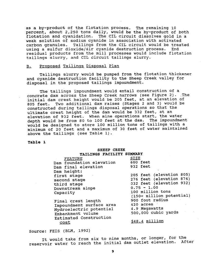
B. Proposed Tailings Disposal Plan 9
C. Other Tailings Disposal Options. Considered . 11
V. AFFECTED ENVIRONMENT 12
A. Introduction 12
B. Sheep Creek Valley.. .... 14
C. Gastineau Channel 15
VI. EVALUATION OF PROJECTED TAILINGS POND PERFORMANCE 17
A. Introduction 17
B. NPDES Requirements 19
C. Review of the FEIS Water Quality Model 20
D. Characteristics of Process Influent to the Tailings
Pond 20
1. FEIS Approach 20
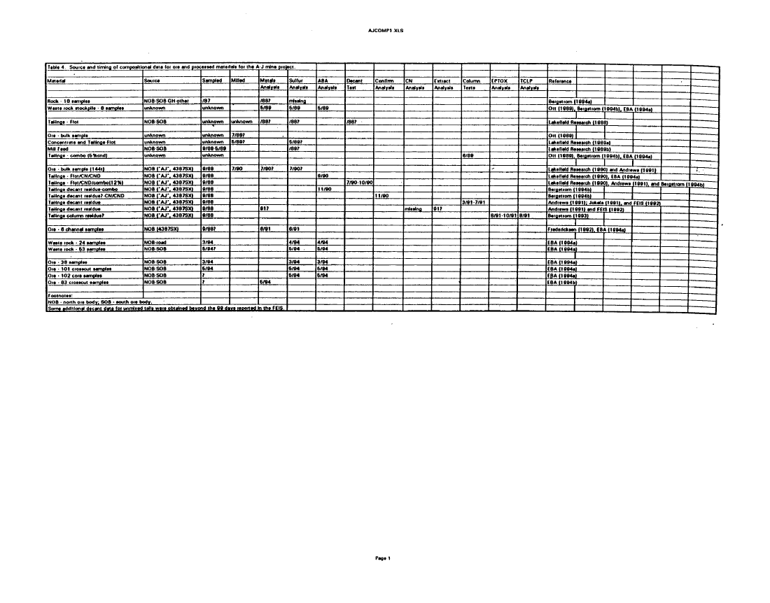
2. Validity of FEIS Approach 21
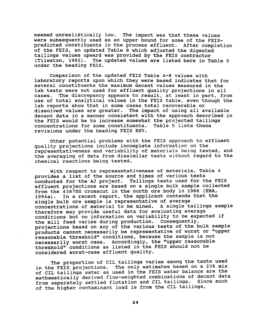
3 . Alternative Approach 26
E. Predictions of Effluent Quality: WASP4 Water Quality
Model 26
1. Introduction. 26
2. Previous Modeling Efforts 27
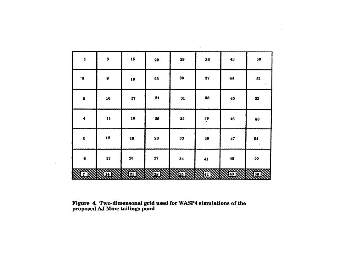
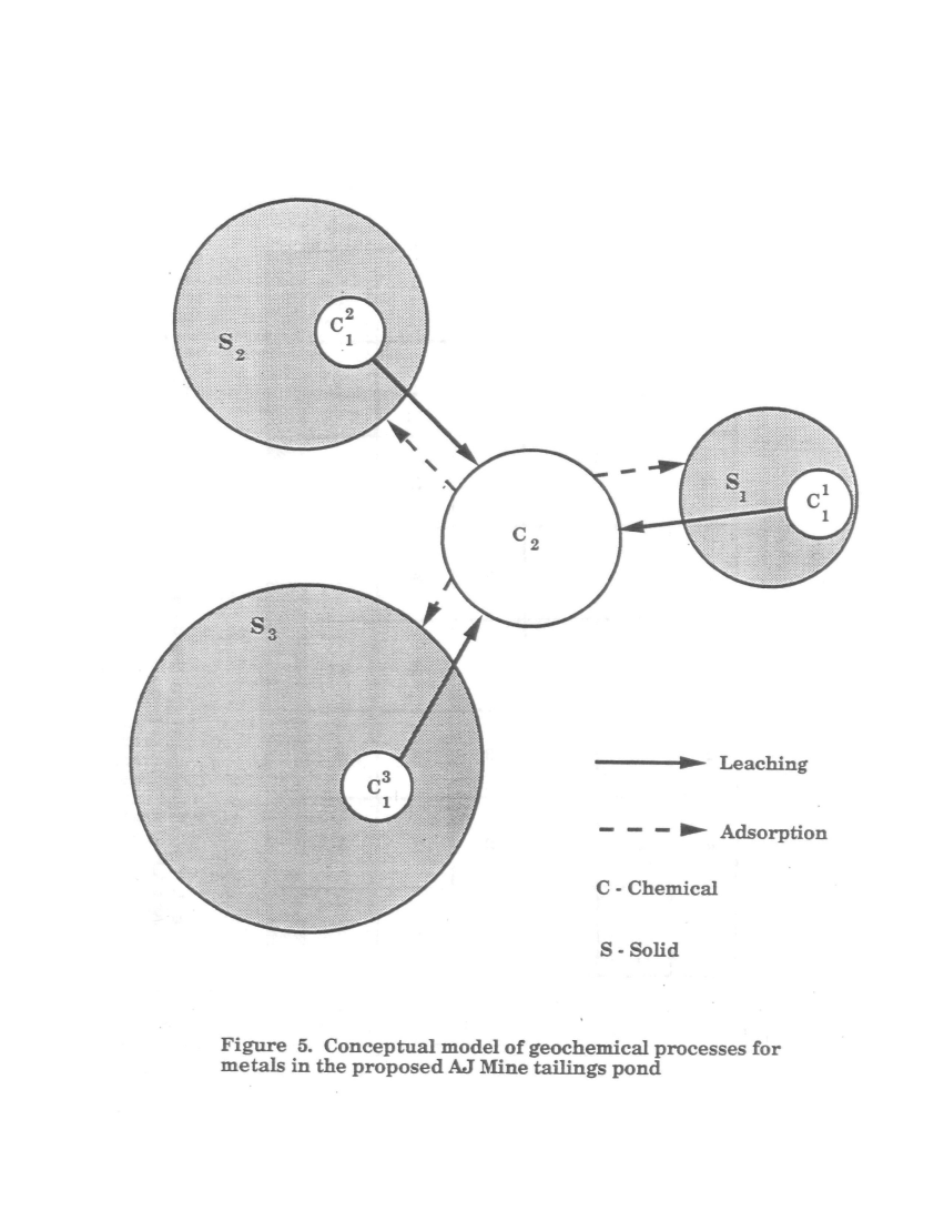
3 . WASP4 Conceptual Model 29
4. Time and Length Scales 33
5. Important Assumptions 33
6. Parameter Estimation 35
7. Simulations 50
8. Results 51
F. Effluent Quality Predictions: CE-QUAL-W2 Water Quality
Model... 57
1. Conceptual Model 57
2. Time and Length Scales 61
3. Important Assumptions 62
4. Parameter Estimation 63
5. Simulations 66
6 Results....••»••••••«•«•••••••••••••••••••••••••••**
G. Discussion of the WASP4 and CE-QUAL-W2 Results 71
H. Comparison with Other Tailings Ponds 85
I. Conclusions Regarding Adequacy of Waste Water
image:
SUMMARY i
I. INTRODUCTION 1
II. SCOPE OF REPORT 4
III. POLICY BACKGROUND 6
IV. PROJECT DESCRIPTION '. 8
A. Mine Location and Processing Operations 8
B. Proposed Tailings Disposal Plan 9
C. Other Tailings Disposal Options. Considered . 11
V. AFFECTED ENVIRONMENT 12
A. Introduction 12
B. Sheep Creek Valley.. .... 14
C. Gastineau Channel 15
VI. EVALUATION OF PROJECTED TAILINGS POND PERFORMANCE 17
A. Introduction 17
B. NPDES Requirements 19
C. Review of the FEIS Water Quality Model 20
D. Characteristics of Process Influent to the Tailings
Pond 20
1. FEIS Approach 20
2. Validity of FEIS Approach 21
3 . Alternative Approach 26
E. Predictions of Effluent Quality: WASP4 Water Quality
Model 26
1. Introduction. 26
2. Previous Modeling Efforts 27
3 . WASP4 Conceptual Model 29
4. Time and Length Scales 33
5. Important Assumptions 33
6. Parameter Estimation 35
7. Simulations 50
8. Results 51
F. Effluent Quality Predictions: CE-QUAL-W2 Water Quality
Model... 57
1. Conceptual Model 57
2. Time and Length Scales 61
3. Important Assumptions 62
4. Parameter Estimation 63
5. Simulations 66
6 Results....••»••••••«•«•••••••••••••••••••••••••••**
G. Discussion of the WASP4 and CE-QUAL-W2 Results 71
H. Comparison with Other Tailings Ponds 85
I. Conclusions Regarding Adequacy of Waste Water
image:
 Treatment ,_ ............................................. 86
VII. POTENTIAL EFFECTS OF THE DISCHARGE ON WATER QUALITY IN
GASTINEAU CHANNEL ........................... .............. 88
A. Introduction ........................................... 88
B. Area Description .............. . ........................ 88
1 . Physical Characteristics ............................ 88
2 . Meteorology ..... . ................................... 90
3 . Freshwater Sources .................................. 90
4. Tidal Influence ..................................... 91
C . Previous Studies ....................................... 92
1. Sewage Outfall Study 1965 ........................... 92
2 . Seawater Monitoring 1989 - 1990 ..................... 92
3 . Channel Current Survey 1990 ......................... 92
4 . Thane Current Survey 1992 ........................... 94
5 . Drift Card Study 1992 ............................... 94
6 . Study Summaries and Comparison ...................... 94
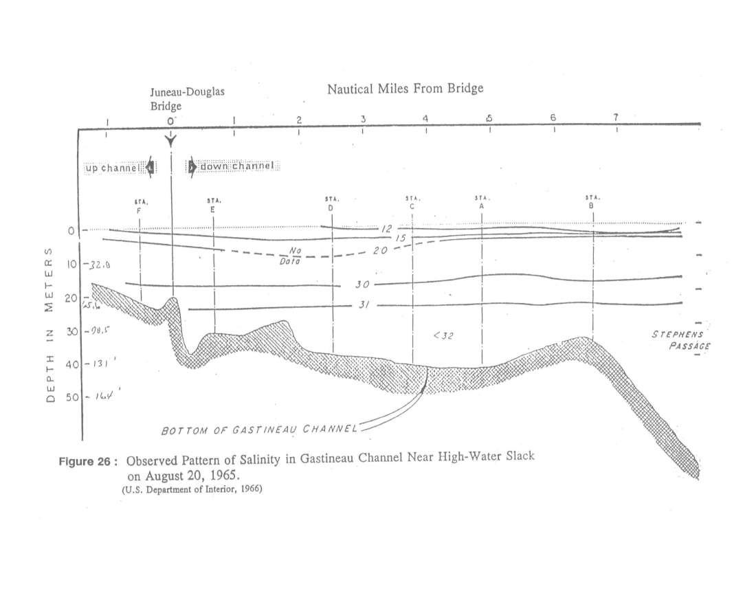
7. Physical Description Summary & Interpretation ....... 98
D. Screening Analysis for Water Quality Impacts ........... 99
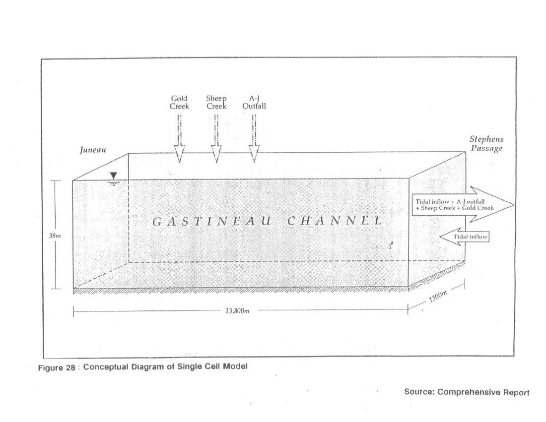
1. Analysis by Echo Bay Alaska ......................... 99
2 . Alternative Screening Analysis ...................... 99
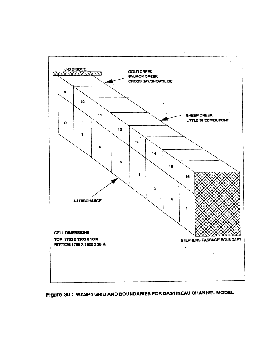
E. Analysis using WASP4 Framework ........................ 102
1 . Introduction ................. . ..................... 102
2 . Model Structure ....... ............................. 103
3 . Model Assumptions .................................. 105
4 . Solution Approach .................................. 105-
5 . Parameter Estimation ........... - ................... 1°6
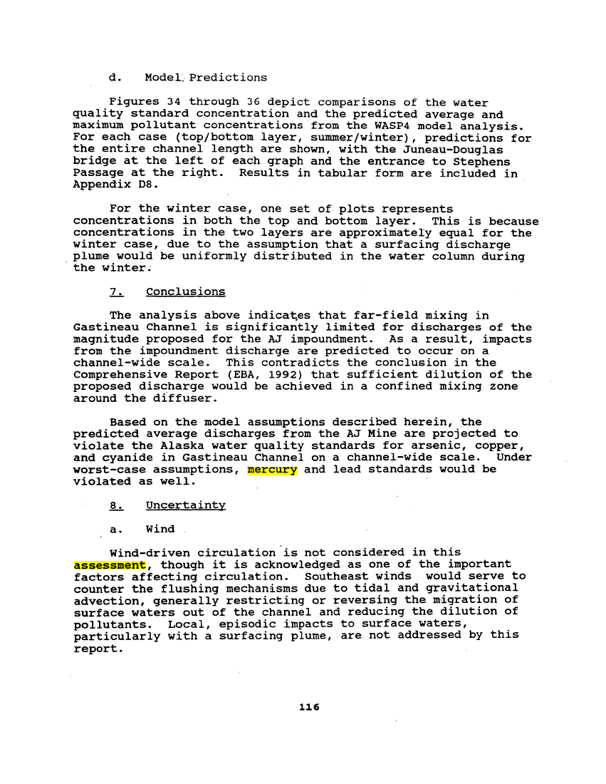
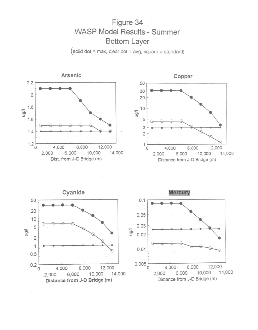
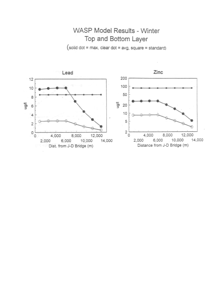
6. Projected Impacts ........ . ......................... 115
7 . Conclusions ........................................ 116
8. Uncertainty ........................................ 116
VIII .RISK OF LONG-TERM CONTAMINATION .......................... 124
A. Introduction
B. Watershed/Physical Setting ........... ................. 124
C. Uncertainty Factors ................... ................ 125
D. Predicted Community Components ........................ 126
1. Benthos ......... ................. '
2 . Plankton.
3. Fish
4 . Macrophytes . . .............................. :
5. Littoral/Riparian (fringe) zone and Vegetation ..... 127
6.
Treatment ,_ ............................................. 86
VII. POTENTIAL EFFECTS OF THE DISCHARGE ON WATER QUALITY IN
GASTINEAU CHANNEL ........................... .............. 88
A. Introduction ........................................... 88
B. Area Description .............. . ........................ 88
1 . Physical Characteristics ............................ 88
2 . Meteorology ..... . ................................... 90
3 . Freshwater Sources .................................. 90
4. Tidal Influence ..................................... 91
C . Previous Studies ....................................... 92
1. Sewage Outfall Study 1965 ........................... 92
2 . Seawater Monitoring 1989 - 1990 ..................... 92
3 . Channel Current Survey 1990 ......................... 92
4 . Thane Current Survey 1992 ........................... 94
5 . Drift Card Study 1992 ............................... 94
6 . Study Summaries and Comparison ...................... 94
7. Physical Description Summary & Interpretation ....... 98
D. Screening Analysis for Water Quality Impacts ........... 99
1. Analysis by Echo Bay Alaska ......................... 99
2 . Alternative Screening Analysis ...................... 99
E. Analysis using WASP4 Framework ........................ 102
1 . Introduction ................. . ..................... 102
2 . Model Structure ....... ............................. 103
3 . Model Assumptions .................................. 105
4 . Solution Approach .................................. 105-
5 . Parameter Estimation ........... - ................... 1°6
6. Projected Impacts ........ . ......................... 115
7 . Conclusions ........................................ 116
8. Uncertainty ........................................ 116
VIII .RISK OF LONG-TERM CONTAMINATION .......................... 124
A. Introduction
B. Watershed/Physical Setting ........... ................. 124
C. Uncertainty Factors ................... ................ 125
D. Predicted Community Components ........................ 126
1. Benthos ......... ................. '
2 . Plankton.
3. Fish
4 . Macrophytes . . .............................. :
5. Littoral/Riparian (fringe) zone and Vegetation ..... 127
6.  Wildlife
 E. Ecological Risk Analysis
F Evaluation of Contaminants in Pore Water
1 Pore Water Evaluated Using Water Quality Criteria. . 129
2. Pore Water Evaluated Using Aquatic Toxicity Data... 13 2
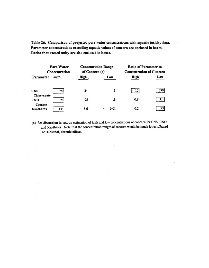
G. Results of Pore Water Evaluation. . ................... • 133
H. Evaluation of Contaminants in Sediments ............... 134
I. Evaluation of Metals in the Water Column .............. 134
image:
E. Ecological Risk Analysis
F Evaluation of Contaminants in Pore Water
1 Pore Water Evaluated Using Water Quality Criteria. . 129
2. Pore Water Evaluated Using Aquatic Toxicity Data... 13 2
G. Results of Pore Water Evaluation. . ................... • 133
H. Evaluation of Contaminants in Sediments ............... 134
I. Evaluation of Metals in the Water Column .............. 134
image:
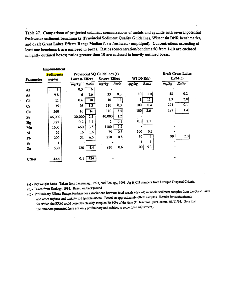
 J. Evaluation of Potential Effects on Wildlife 137
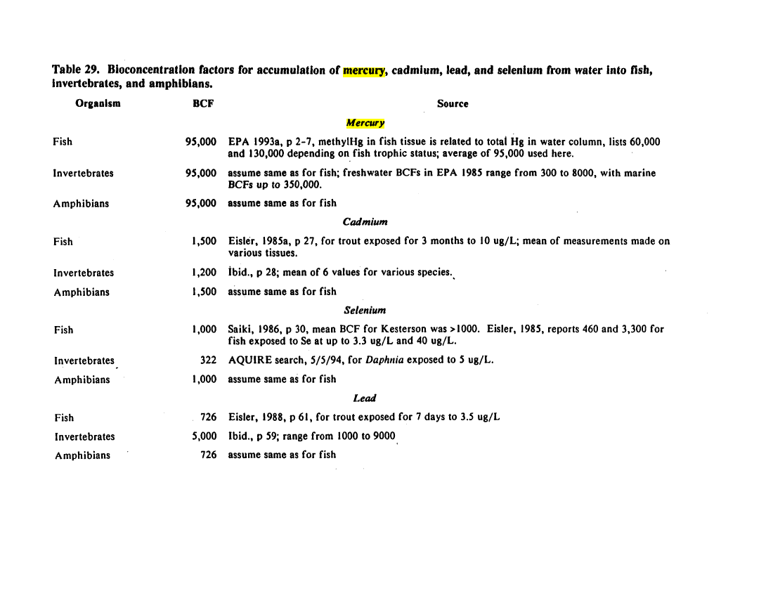
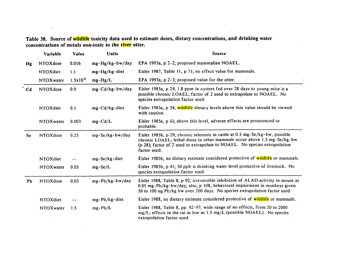
1. Selection of Contaminants 137
2 . Selection of Species 137
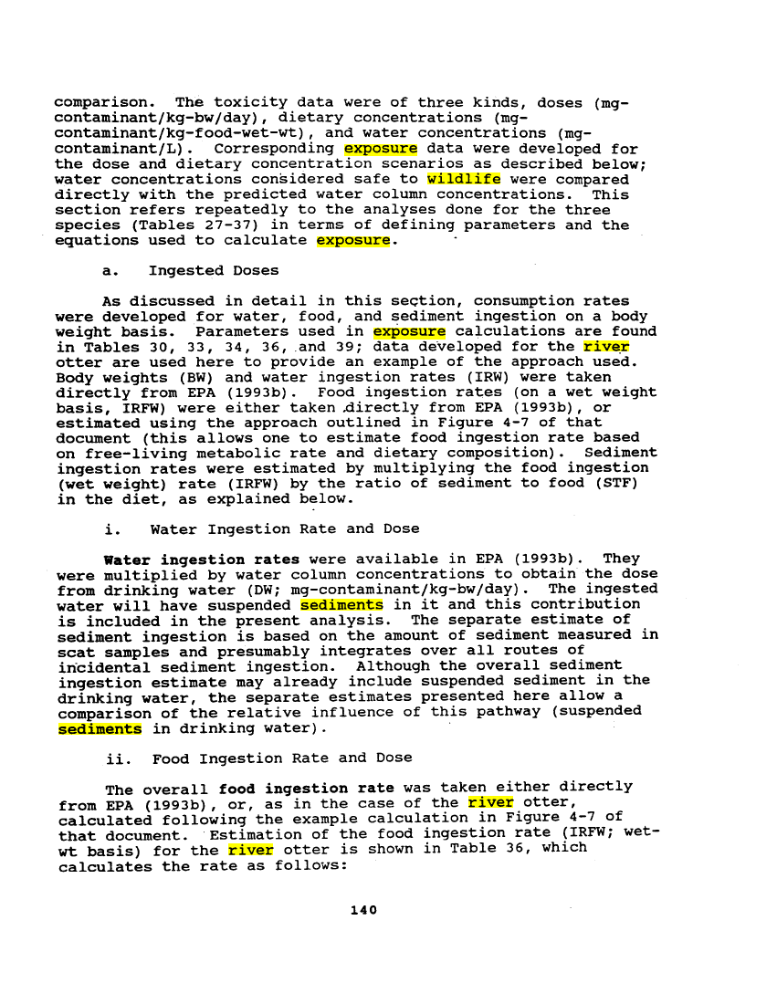
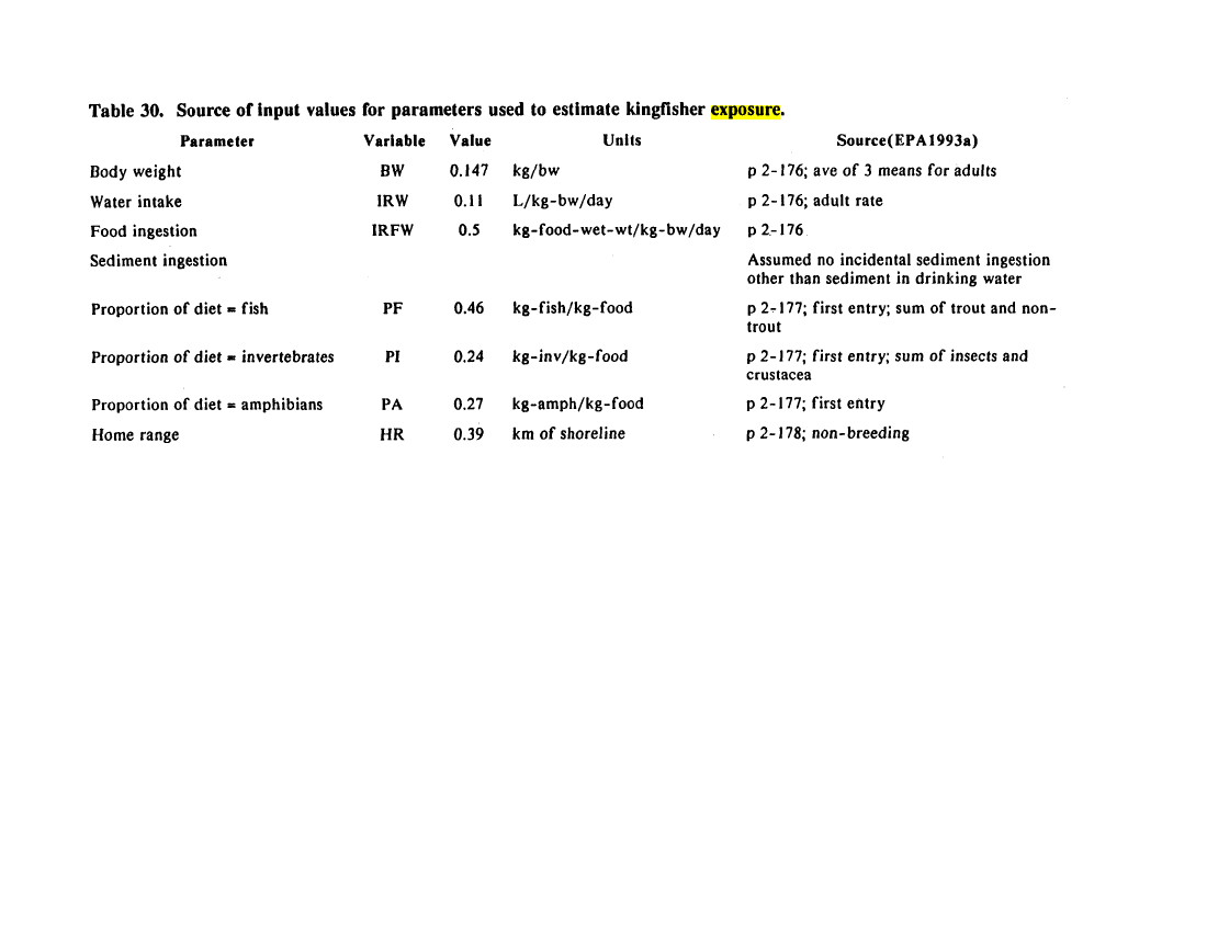
3 . Selection of Exposure Pathways 139
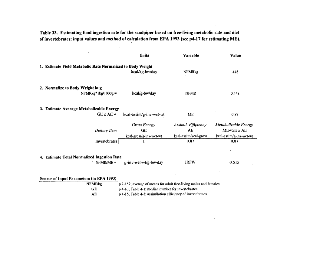
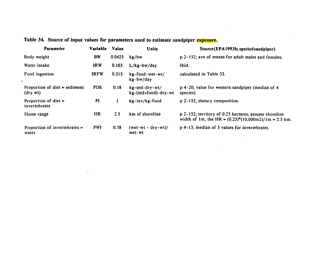
4 . Exposure of Wildlife to Metals 139
5. Kingfisher - Exposure, Toxicity, and Effect 159
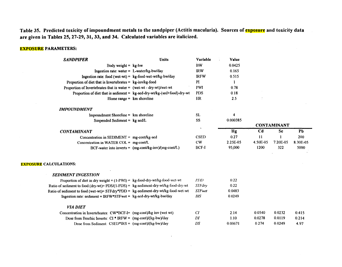
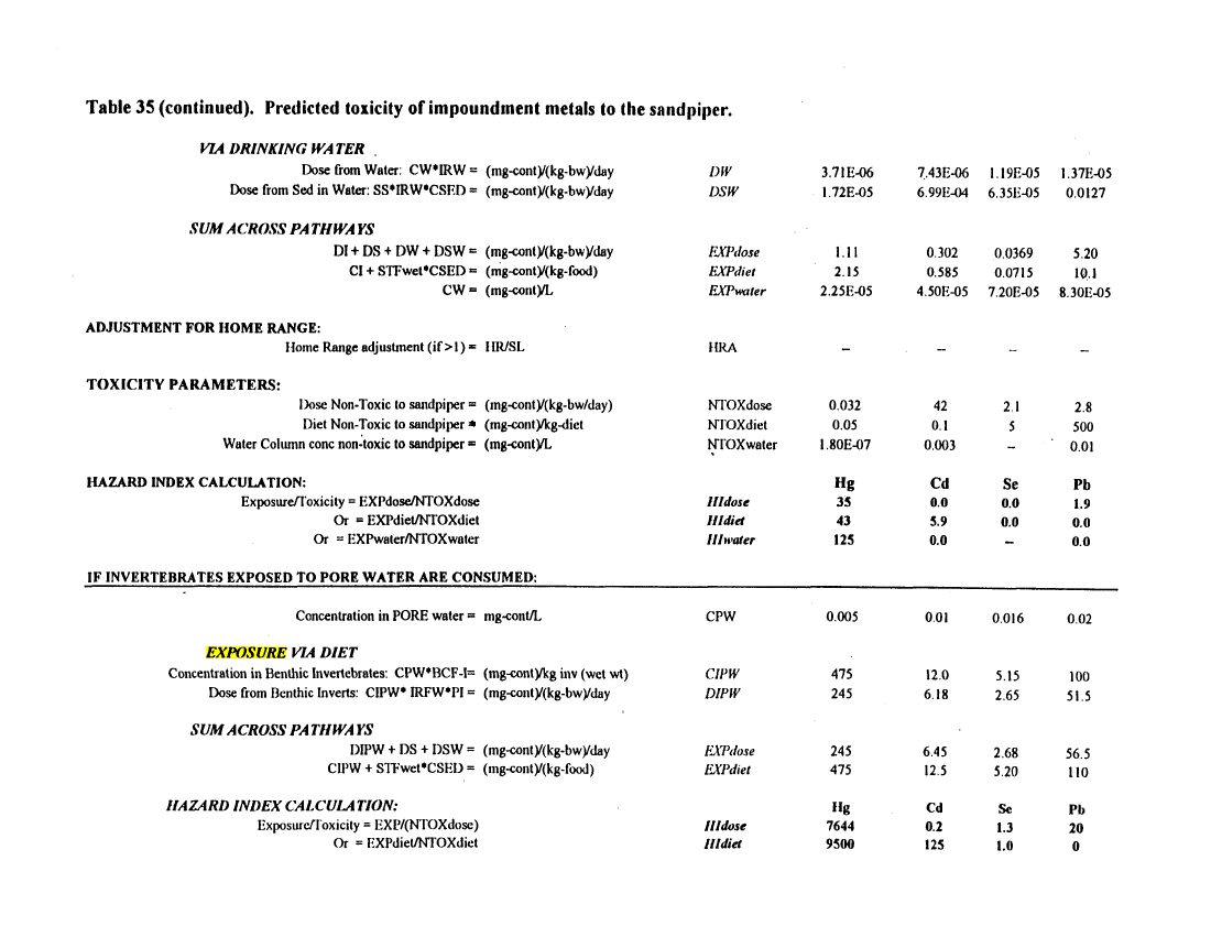
6. Exposure and Toxicity to the Sandpiper 159
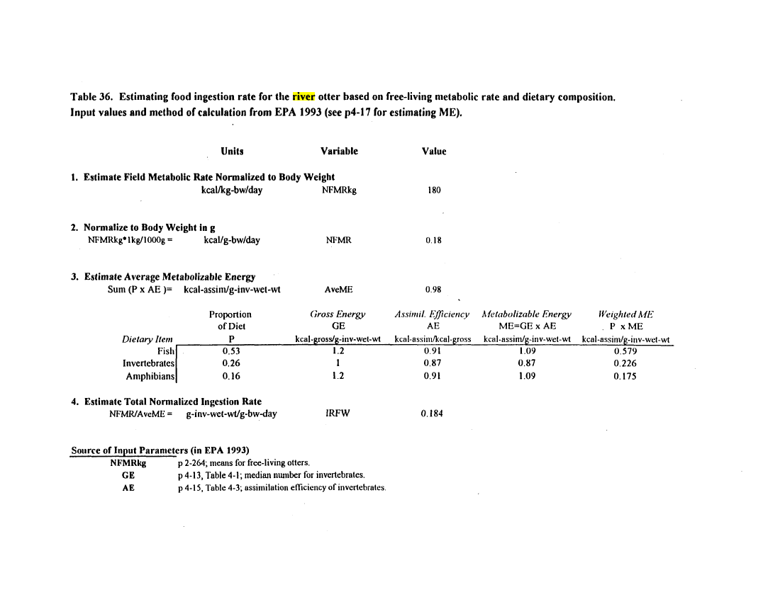
7. Exposure and Toxicity to the River Otter....; 160
K. Uncertainty Factors • 160
L. Summary of Ecology Risk Analysis 162
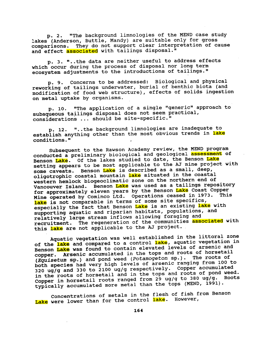
M. Review of Literature on Subaqueous Disposal of Mine
Tailings 163
N. Laboratory Tests Relevant to the Long-Term Behaviour of
Metals and Other Constituents 165
1. Leach Tests 165
2 . Acid Generation Potential 166
O. Conclusions Regarding Potential Long-Term
contamination 167
IX. POTENTIAL MEASURES TO MITIGATE WATER QUALITY IMPACTS 170
A. Introduction. 170
B. Secondary Wastewater Treatment 170
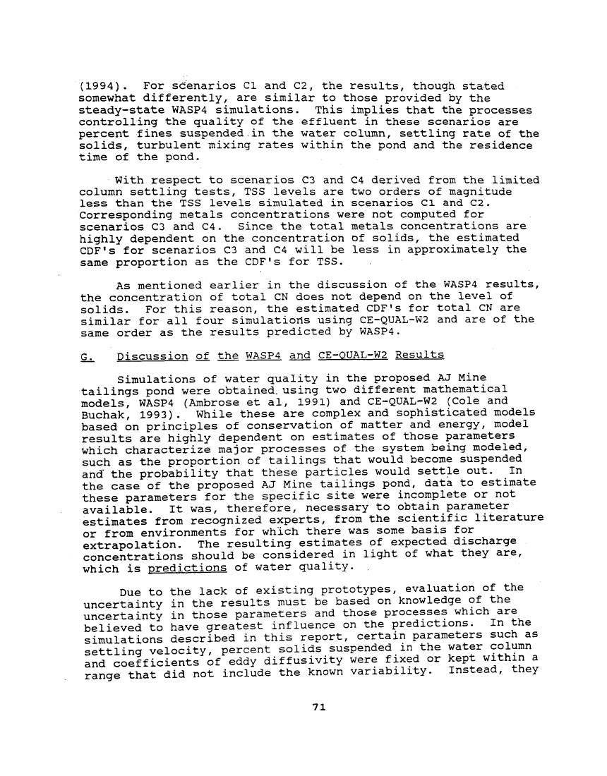
C. Potential Measures for Reducing TSS 171
D. Isolating the Tailings.... 171
E. Eliminating the Cyanide Leach Circuit _ 172
F. Alternative Tailings Disposal Sites 172
X. POTENTIAL MEASURES TO MITIGATE ECOLOGICAL IMPACTS 174
A. Introduction 174
B. On-site Mitigation Proposals 175
C. Off-site Mitigation Proposals 175
D. Mitigation for Lost Values in Marine Waters 177
E. Conclusion .177
XI. CONCLUSIONS 178
XII. REFERENCES 180
XIII.LIST OF PREPARERS 189
image:
J. Evaluation of Potential Effects on Wildlife 137
1. Selection of Contaminants 137
2 . Selection of Species 137
3 . Selection of Exposure Pathways 139
4 . Exposure of Wildlife to Metals 139
5. Kingfisher - Exposure, Toxicity, and Effect 159
6. Exposure and Toxicity to the Sandpiper 159
7. Exposure and Toxicity to the River Otter....; 160
K. Uncertainty Factors • 160
L. Summary of Ecology Risk Analysis 162
M. Review of Literature on Subaqueous Disposal of Mine
Tailings 163
N. Laboratory Tests Relevant to the Long-Term Behaviour of
Metals and Other Constituents 165
1. Leach Tests 165
2 . Acid Generation Potential 166
O. Conclusions Regarding Potential Long-Term
contamination 167
IX. POTENTIAL MEASURES TO MITIGATE WATER QUALITY IMPACTS 170
A. Introduction. 170
B. Secondary Wastewater Treatment 170
C. Potential Measures for Reducing TSS 171
D. Isolating the Tailings.... 171
E. Eliminating the Cyanide Leach Circuit _ 172
F. Alternative Tailings Disposal Sites 172
X. POTENTIAL MEASURES TO MITIGATE ECOLOGICAL IMPACTS 174
A. Introduction 174
B. On-site Mitigation Proposals 175
C. Off-site Mitigation Proposals 175
D. Mitigation for Lost Values in Marine Waters 177
E. Conclusion .177
XI. CONCLUSIONS 178
XII. REFERENCES 180
XIII.LIST OF PREPARERS 189
image:
 APPENDICES (Bound Separately)
APPENDIX A to Chapter III: Policy Background
APPENDIX Al: EPA memo of October 2, 1992
APPENDIX A2: Clean Water Act §404(b)(l) Guidelines
APPENDIX B to Chapter VI: Tailings Pond influent
APPENDIX Bl: Table B-l
APPENDIX B2: Table B-2
APPENDIX C to Chapter VI: Water Quality Modeling
APPENDIX Cl: GROUNDWATER FLOW
APPENDIX C2: WASP4 INPUT
APPENDIX C3: CE-QUAL-W2 INPUT
APPENDIX D to Chapter VII: Water Quality in Gastineau Channel
APPENDIX Dl: AMBIENT WATER QUALITY DATA
- Salinity Data
- Metals in Gastineau Channel
APPENDIX D2: TIDAL INFORMATION
- Tidal Charts
- WASP4 Input Flows
APPENDIX D3: CURRENT METER DATA (excerpts)
APPENDIX D4: FRESHWATER SCALING
APPENDIX D5: DILUTION MODELING
APPENDIX D6: WASP4 INPUT FILES
APPENDIX D7: WASP4 TIME SERIES PLOTS
APPENDIX D8: RESULTS IN TABULAR FORM
APPENDIX D9: DROGUE AND DRIFT CARD SURVEYS
- Echo Bay Survey Diagrams
- NMFS Draft Report (complete)
APPENDIX E to Chapters IX and X: Potential Mitigation Measures
APPENDIX El: Upstream Diversion Dam
APPENDIX E2: Treatment Facility Mitigation Measures
image:
APPENDICES (Bound Separately)
APPENDIX A to Chapter III: Policy Background
APPENDIX Al: EPA memo of October 2, 1992
APPENDIX A2: Clean Water Act §404(b)(l) Guidelines
APPENDIX B to Chapter VI: Tailings Pond influent
APPENDIX Bl: Table B-l
APPENDIX B2: Table B-2
APPENDIX C to Chapter VI: Water Quality Modeling
APPENDIX Cl: GROUNDWATER FLOW
APPENDIX C2: WASP4 INPUT
APPENDIX C3: CE-QUAL-W2 INPUT
APPENDIX D to Chapter VII: Water Quality in Gastineau Channel
APPENDIX Dl: AMBIENT WATER QUALITY DATA
- Salinity Data
- Metals in Gastineau Channel
APPENDIX D2: TIDAL INFORMATION
- Tidal Charts
- WASP4 Input Flows
APPENDIX D3: CURRENT METER DATA (excerpts)
APPENDIX D4: FRESHWATER SCALING
APPENDIX D5: DILUTION MODELING
APPENDIX D6: WASP4 INPUT FILES
APPENDIX D7: WASP4 TIME SERIES PLOTS
APPENDIX D8: RESULTS IN TABULAR FORM
APPENDIX D9: DROGUE AND DRIFT CARD SURVEYS
- Echo Bay Survey Diagrams
- NMFS Draft Report (complete)
APPENDIX E to Chapters IX and X: Potential Mitigation Measures
APPENDIX El: Upstream Diversion Dam
APPENDIX E2: Treatment Facility Mitigation Measures
image:
 APPENDIX E3: Post-Mine Closure Measures
APPENDIX E4: Ecological Impact Measures
image:
APPENDIX E3: Post-Mine Closure Measures
APPENDIX E4: Ecological Impact Measures
image:
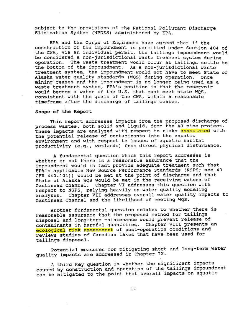
 SUMMARY
Project Description
The Alaska Juneau (AJ) Gold Mine project is a proposal by
Echo Bay Alaska (Echo Bay) to reopen the historic AJ gold mine
near Juneau in southeast Alaska. The proposal entails mining
approximately 22,500 tons of ore per day and, after crushing and
grinding the ore, recovering gold through the froth flotation and
carbon-in-leach (CIL; also referred to as cyanide leach)
processes. After destruction of residual cyanide in the CIL
tailings using a sulfur dioxide/air process, the tailings would
then be discharged in .a slurry form to a tailings impoundment
that would be created in Sheep Creek valley, four miles south of
downtown Juneau.
Echo. Bay proposes to construct a 345' high roller compacted
concrete dam that would create a reservoir approximately 2.5
miles long in Sheep Creek valley. Tailings would be discharged
into this impoundment via a barge mounted "elephant trunk"
tailings discharge pipeline extending to the bottom of the
reservoir. During operation, mine drainage water and process
water, equivalent in volume to the net precipitation (after
evaporation) over the impoundment, would be discharged from the
impoundment to Gastineau Channel, approximately one mile to the
west of the tailings impoundment.
The tailings impoundment would serve as a permanent disposal
site for the AJ mine tailings. Echo Bay's proposal is to leave a
minimum of twenty feet of water over the tailings and, after
mining and tailings disposal cease, to allow the impoundment to
serve as a. recreational lake. A more complete project
description can be found in the AJ Gold Mine Project Final
Environmental Impact Statement (FEIS; BLM, 1992).
Regulatory Background
This report evaluates short and long-term water quality
impacts from the project as well as long-term ecological
consequences. Findings and recommendations have been developed
to assist the Alaska District Corps of Engineers in determining
whether the proposed project complies with the Clean Water Act
(CWA) Section 404(b)(l) Guidelines.
A CWA Section 404 permit is required to place fill for
construction of the tailings impoundment, which is intended to
function as a wastewater treatment system. These permits are
issued by the Corps of Engineers with the assistance of EPA.
A CWA section 402 permit would be required during operation for
the discharge of wastewater from the impoundment (as well as mine
drainage) to Gastineau Channel. CWA section 402 permits are
image:
SUMMARY
Project Description
The Alaska Juneau (AJ) Gold Mine project is a proposal by
Echo Bay Alaska (Echo Bay) to reopen the historic AJ gold mine
near Juneau in southeast Alaska. The proposal entails mining
approximately 22,500 tons of ore per day and, after crushing and
grinding the ore, recovering gold through the froth flotation and
carbon-in-leach (CIL; also referred to as cyanide leach)
processes. After destruction of residual cyanide in the CIL
tailings using a sulfur dioxide/air process, the tailings would
then be discharged in .a slurry form to a tailings impoundment
that would be created in Sheep Creek valley, four miles south of
downtown Juneau.
Echo. Bay proposes to construct a 345' high roller compacted
concrete dam that would create a reservoir approximately 2.5
miles long in Sheep Creek valley. Tailings would be discharged
into this impoundment via a barge mounted "elephant trunk"
tailings discharge pipeline extending to the bottom of the
reservoir. During operation, mine drainage water and process
water, equivalent in volume to the net precipitation (after
evaporation) over the impoundment, would be discharged from the
impoundment to Gastineau Channel, approximately one mile to the
west of the tailings impoundment.
The tailings impoundment would serve as a permanent disposal
site for the AJ mine tailings. Echo Bay's proposal is to leave a
minimum of twenty feet of water over the tailings and, after
mining and tailings disposal cease, to allow the impoundment to
serve as a. recreational lake. A more complete project
description can be found in the AJ Gold Mine Project Final
Environmental Impact Statement (FEIS; BLM, 1992).
Regulatory Background
This report evaluates short and long-term water quality
impacts from the project as well as long-term ecological
consequences. Findings and recommendations have been developed
to assist the Alaska District Corps of Engineers in determining
whether the proposed project complies with the Clean Water Act
(CWA) Section 404(b)(l) Guidelines.
A CWA Section 404 permit is required to place fill for
construction of the tailings impoundment, which is intended to
function as a wastewater treatment system. These permits are
issued by the Corps of Engineers with the assistance of EPA.
A CWA section 402 permit would be required during operation for
the discharge of wastewater from the impoundment (as well as mine
drainage) to Gastineau Channel. CWA section 402 permits are
image:
 subject to the provisions of the National Pollutant Discharge
Elimination System (NPDES) administered by EPA.
EPA and the Corps of Engineers have agreed that if the
construction of the impoundment is permitted under Section 404 of
the CWA, via an individual permit, the tailings impoundment would
be considered a non-jurisdictional waste treament system during
operation. The waste treatment would occur as tailings- settle to
the bottom of the impoundment. As a non-jurisdictional waste
treatment system, the impoundment would not have to meet State of
Alaska water quality standards (WQS) during operation. Once
mining ceases and the impoundment is no longer being used as a
waste treatment system, EPA's position is that the reservoir
would become a water of the U.S. that must meet state WQS,
consistent with the goals of the CWA, within a reasonable
timefra.me after the discharge of tailings ceases.
Scope of the Report
This report addresses impacts from the proposed discharge of
process wastes, both solid and liquid, from the AJ mine project.
These impacts are analyzed witn respect to risks associated with
the potential release of contaminants into the aquatic
environment and with respect to losses of aquatic habitat
productivity (e.g., wetlands) from direct physical disturbance.
A fundamental question which this report addresses is
whether or not there is a reasonable assurance that the
impoundment would in fact provide adequate treatment such that
EPA's applicable New Source Performance Standards (NSPS; see 40
CFR 440.104)) would be met at the point of discharge and that
State of Alaska WQS would be met in the receiving waters of
Gastineau Channel. Chapter VI addresses this question with
respect to NSPS, relying heavily on water quality modeling
analyses. Chapter VII addresses overall water quality impacts to
Gastineau Channel and the likelihood of meeting WQS.
Another fundamental question relates to whether there is
reasonable assurance that the proposed method for tailings
disposal and long-term maintenance would prevent release of
contaminants in harmful quantities. Chapter VIII presents an
ecological risk assessment of post-operation conditions and
reviews studies of Canadian lakes that have been used for
tailings disposal.
Potential measures for mitigating short and long-term water
quality impacts are addressed in Chapter IX.
A third key question is whether the significant impacts
caused by construction and operation of the tailings impoundment
can be mitigated to the point that overall impacts on aquatic
ii
image:
subject to the provisions of the National Pollutant Discharge
Elimination System (NPDES) administered by EPA.
EPA and the Corps of Engineers have agreed that if the
construction of the impoundment is permitted under Section 404 of
the CWA, via an individual permit, the tailings impoundment would
be considered a non-jurisdictional waste treament system during
operation. The waste treatment would occur as tailings- settle to
the bottom of the impoundment. As a non-jurisdictional waste
treatment system, the impoundment would not have to meet State of
Alaska water quality standards (WQS) during operation. Once
mining ceases and the impoundment is no longer being used as a
waste treatment system, EPA's position is that the reservoir
would become a water of the U.S. that must meet state WQS,
consistent with the goals of the CWA, within a reasonable
timefra.me after the discharge of tailings ceases.
Scope of the Report
This report addresses impacts from the proposed discharge of
process wastes, both solid and liquid, from the AJ mine project.
These impacts are analyzed witn respect to risks associated with
the potential release of contaminants into the aquatic
environment and with respect to losses of aquatic habitat
productivity (e.g., wetlands) from direct physical disturbance.
A fundamental question which this report addresses is
whether or not there is a reasonable assurance that the
impoundment would in fact provide adequate treatment such that
EPA's applicable New Source Performance Standards (NSPS; see 40
CFR 440.104)) would be met at the point of discharge and that
State of Alaska WQS would be met in the receiving waters of
Gastineau Channel. Chapter VI addresses this question with
respect to NSPS, relying heavily on water quality modeling
analyses. Chapter VII addresses overall water quality impacts to
Gastineau Channel and the likelihood of meeting WQS.
Another fundamental question relates to whether there is
reasonable assurance that the proposed method for tailings
disposal and long-term maintenance would prevent release of
contaminants in harmful quantities. Chapter VIII presents an
ecological risk assessment of post-operation conditions and
reviews studies of Canadian lakes that have been used for
tailings disposal.
Potential measures for mitigating short and long-term water
quality impacts are addressed in Chapter IX.
A third key question is whether the significant impacts
caused by construction and operation of the tailings impoundment
can be mitigated to the point that overall impacts on aquatic
ii
image:
 resources are acceptable. Optional mitigation plans and
strategies are-reviewed in Chapter X.
Affected Environment
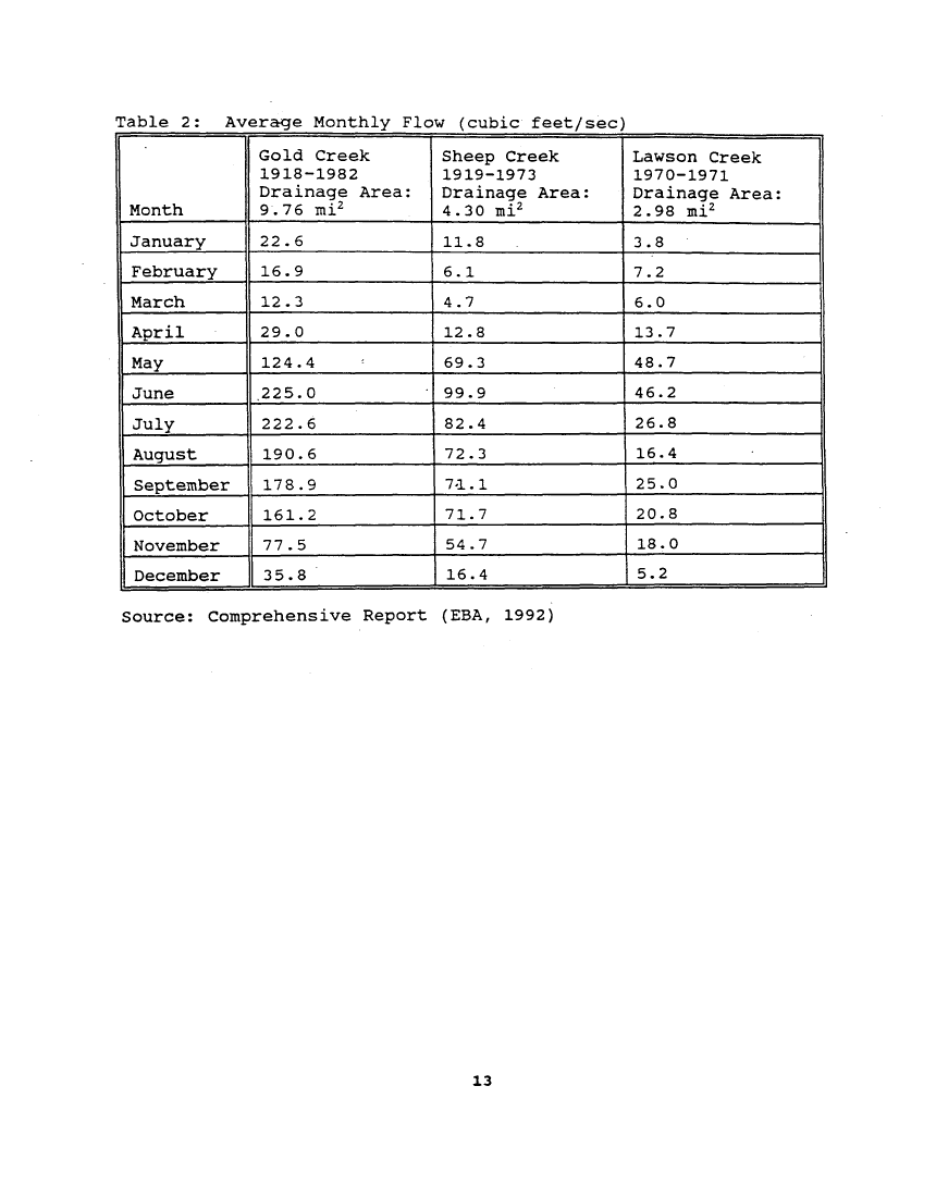
The Sheep Creek tailings disposal option would fill 420
acres of Sheep Creek valley. Waters that would be eliminated in
association with the proposed fill are 2.5 miles of Sheep Creek
above the tailings dam and associated wetlands for a total of
20.1 acres of aquatic habitat (COE, 1994). The flow of water in
1.1 additional miles of Sheep Creek downstream of the impoundment
would be reduced significantly.
Mammals that inhabit the immediate area include black bear,
mountain goat, Sitka black-tailed deer, beaver, marten, river
otter, mink, ermine, and other mustelids, lynx, red fox, hoary
marmot, porcupine and other small mammals (Holmberg, 1991).
There are 131 species of birds that likely inhabit the project
area for at least some time of the year. Among these are bald
and golden eagles as well as more than a dozen neotropical.
migratory song birds and shore birds (Wilson and Comet, 1991).
The wetlands of Sheep Creek valley are an element of a
diverse mosaic of vegetation communities which the FEIS describes
as unique among the alternative tailings disposal sites
considered. Due to this vegetation mosaic, the FEIS describes
the Sheep Creek valley as having more species diversity than any
other site accessible on the Juneau road system. The wetlands
serve basic ecological functions within this mosaic typical of
wetlands at other locations. However, the upper portion of Sheep
Creek valley is unusual for the Juneau area because of the
composition of its vegetative communities. Vegetation consists
of coniferous forest, deciduous forest, tall shrub, upland
meadow, shrub wetland and wet meadow. The deciduous forest,
composed primarily of cottonwood, is uncommon in the greater
Juneau area. Rough estimates suggest that Sheep Creek Valley
contains 25% of the total area of cottonwoods between Taku Inlet
and Berners Bay (BLM, 1992).
The mixture of cottonwood and wetland shrub communities
apparently provides a high quality habitat for song birds. Song
bird populations have been found to be "locally diverse and
abundant" (Wilson and Comet, 1991). Sheep Creek valley had five
times the song bird nest density and over 323% more successful
nests than a nearby site with similar vegetation (Comet and
Wilson, 1994) . Habitats adjacent to the valley floor have
notably fewer songbirds (Wilson and Comet, 1993). Many of the
song bird species are of special interest. Five species whose
abundance is thought to be in decline in Alaska breed in the
valley. These are the fox sparrow, orange crowned warbler,
blackpoll warbler, American robin, and varied thrush. Eight
other species found in the valley may be increasing in abundance.
iii
image:
resources are acceptable. Optional mitigation plans and
strategies are-reviewed in Chapter X.
Affected Environment
The Sheep Creek tailings disposal option would fill 420
acres of Sheep Creek valley. Waters that would be eliminated in
association with the proposed fill are 2.5 miles of Sheep Creek
above the tailings dam and associated wetlands for a total of
20.1 acres of aquatic habitat (COE, 1994). The flow of water in
1.1 additional miles of Sheep Creek downstream of the impoundment
would be reduced significantly.
Mammals that inhabit the immediate area include black bear,
mountain goat, Sitka black-tailed deer, beaver, marten, river
otter, mink, ermine, and other mustelids, lynx, red fox, hoary
marmot, porcupine and other small mammals (Holmberg, 1991).
There are 131 species of birds that likely inhabit the project
area for at least some time of the year. Among these are bald
and golden eagles as well as more than a dozen neotropical.
migratory song birds and shore birds (Wilson and Comet, 1991).
The wetlands of Sheep Creek valley are an element of a
diverse mosaic of vegetation communities which the FEIS describes
as unique among the alternative tailings disposal sites
considered. Due to this vegetation mosaic, the FEIS describes
the Sheep Creek valley as having more species diversity than any
other site accessible on the Juneau road system. The wetlands
serve basic ecological functions within this mosaic typical of
wetlands at other locations. However, the upper portion of Sheep
Creek valley is unusual for the Juneau area because of the
composition of its vegetative communities. Vegetation consists
of coniferous forest, deciduous forest, tall shrub, upland
meadow, shrub wetland and wet meadow. The deciduous forest,
composed primarily of cottonwood, is uncommon in the greater
Juneau area. Rough estimates suggest that Sheep Creek Valley
contains 25% of the total area of cottonwoods between Taku Inlet
and Berners Bay (BLM, 1992).
The mixture of cottonwood and wetland shrub communities
apparently provides a high quality habitat for song birds. Song
bird populations have been found to be "locally diverse and
abundant" (Wilson and Comet, 1991). Sheep Creek valley had five
times the song bird nest density and over 323% more successful
nests than a nearby site with similar vegetation (Comet and
Wilson, 1994) . Habitats adjacent to the valley floor have
notably fewer songbirds (Wilson and Comet, 1993). Many of the
song bird species are of special interest. Five species whose
abundance is thought to be in decline in Alaska breed in the
valley. These are the fox sparrow, orange crowned warbler,
blackpoll warbler, American robin, and varied thrush. Eight
other species found in the valley may be increasing in abundance.
iii
image:
 Fifteen of the 42 species of birds documented during formal
censusing are o'f interest to the national program on neotropical
birds (Wilson and. Comet, 1991) . One bird, the marbled murrelet,
whose use of the valley has not been documented, is of concern
because of population declines along the west coast of North
America.
Aquatic resources of the upper portion of Sheep Creek
include a local population of Dolly Vardon char. This population
is isolated from other char populations by .the impassible lower
reach of Sheep Creek.
Gastineau Channel is a north-south oriented channel
separating Douglas Island from the mainland. The shoreline for
approximately 10 miles between Stephens Passage and Juneau is
largely steep sided and rocky. Forty species of demersal fish,
shellfish and other invertebrates have been reported from
Gastineau Channel. Included among these are commercially
"important crab species. The commercial crab fishery was closed
in 1978 but a popular personal use fishery continues (BLM, 1992).
Adequacy of Wastewater Treatment
Chapter VI addresses the projected performance of the
tailings impoundment as a waste treatment system. Water quality
models and information from existing mines are used to determine
whether the discharge from the impoundment, when comingled with
mine drainage, would be likely to meet EPA's New Source
Performance Standards (NSPS) that would apply to the discharge as
end-of-pipe effluent limits. Compliance with Alaska's water
quality standards (WQS) is addressed in Chapter VII.
The chemical composition of the tailings slurry discharge is
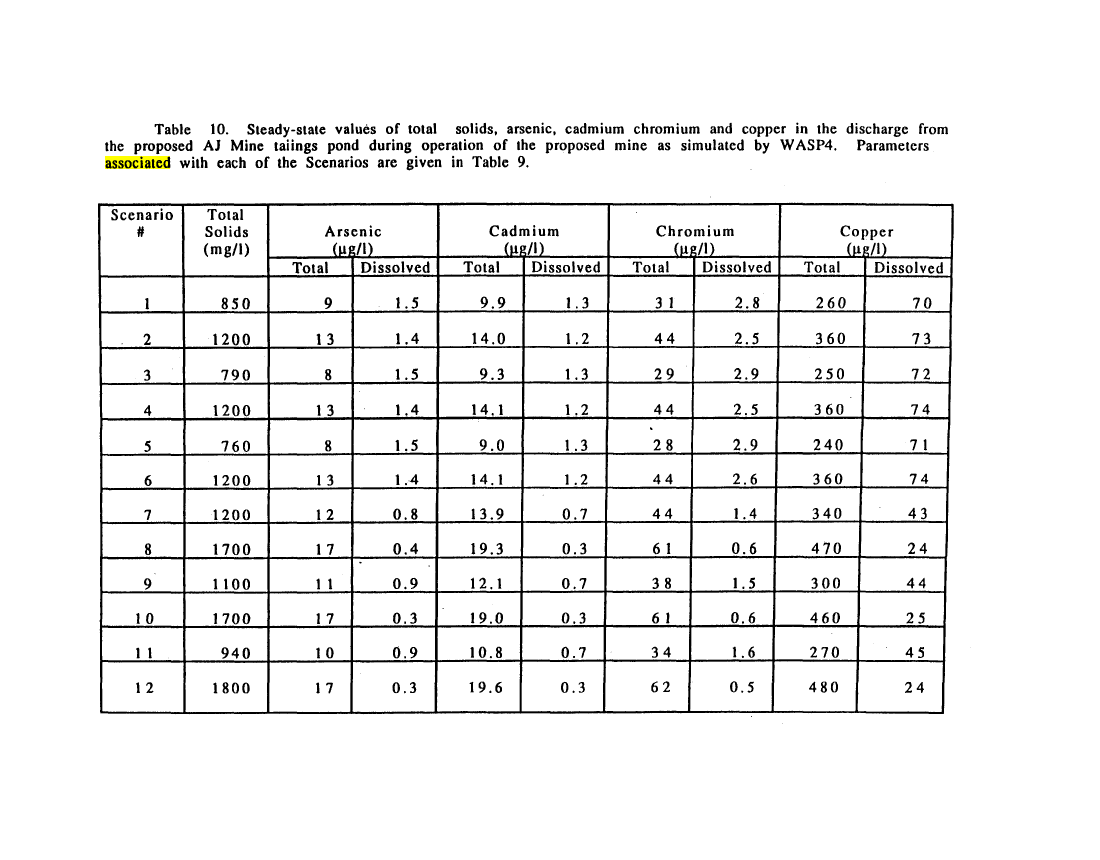
discussed. Concentrations of various chemical constituents of
the influent to the tailings pond are presented. They represent
the pollutant loadings to the tailings pond that are subsequently
addressed in water quality models.
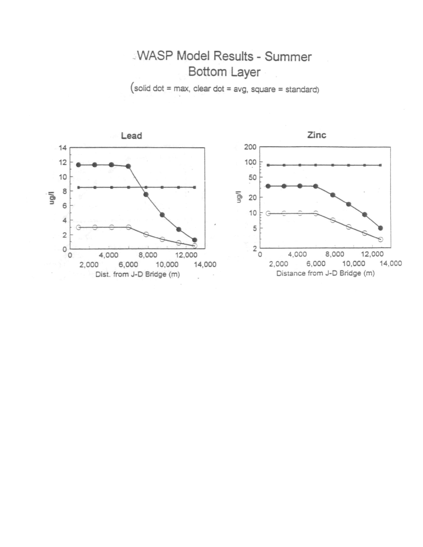
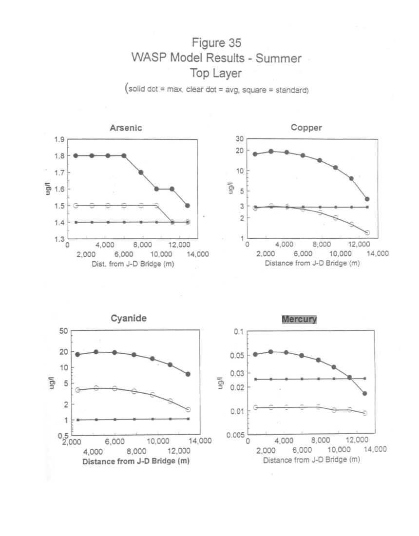
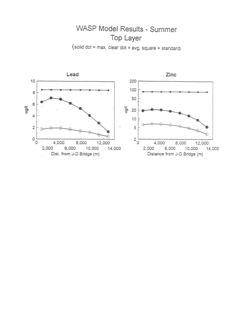
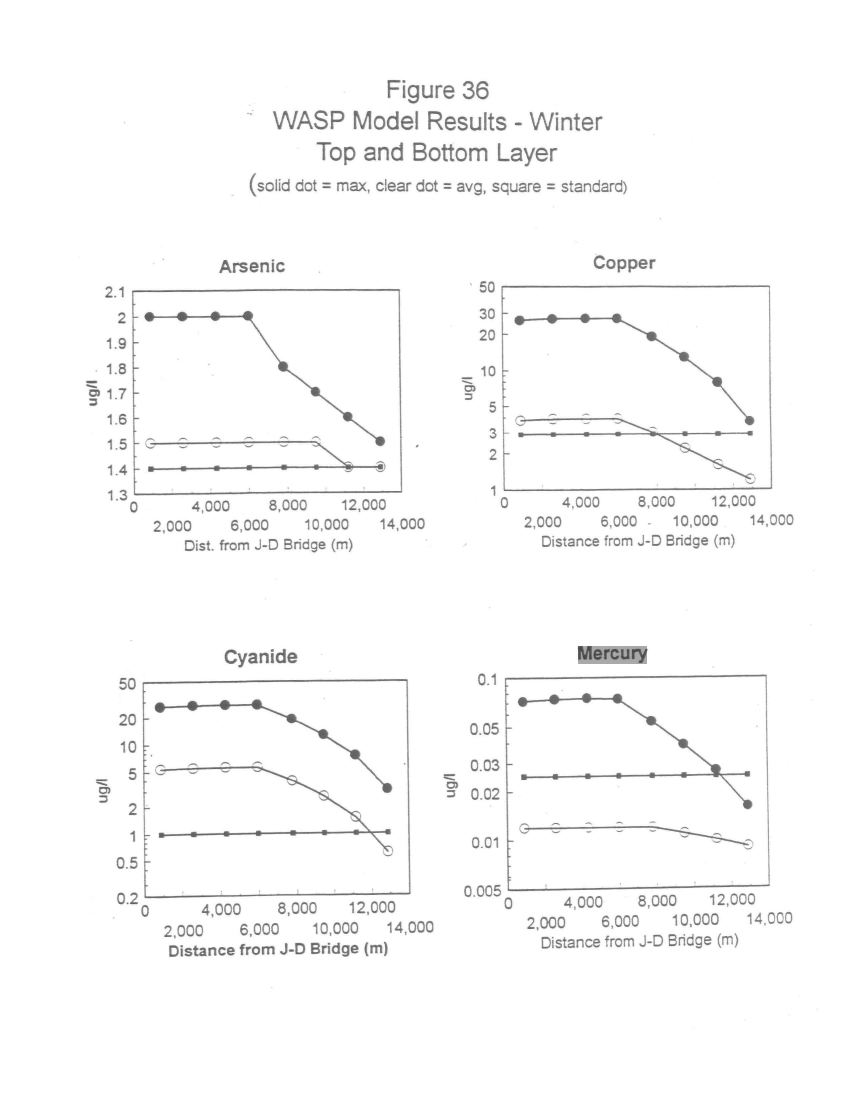
Two water quality models were applied to estimate the levels
of pollutants that would be expected in the discharge. The EPA's
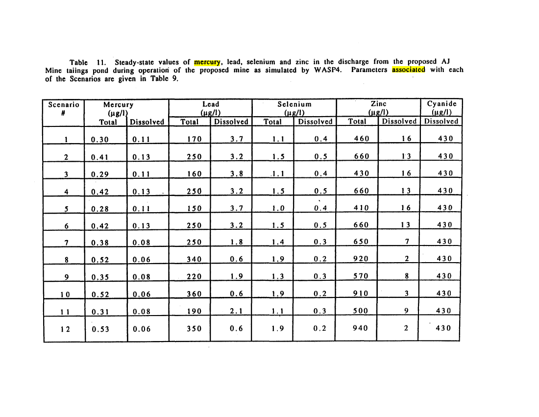
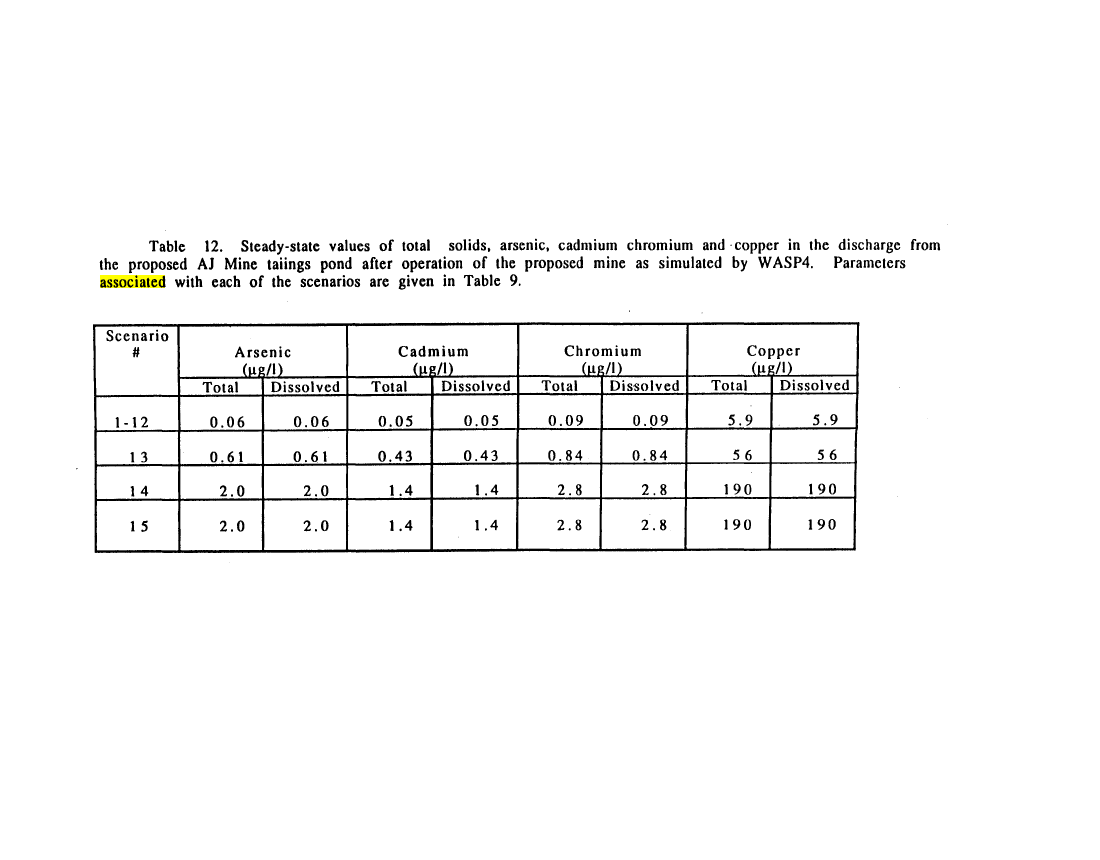
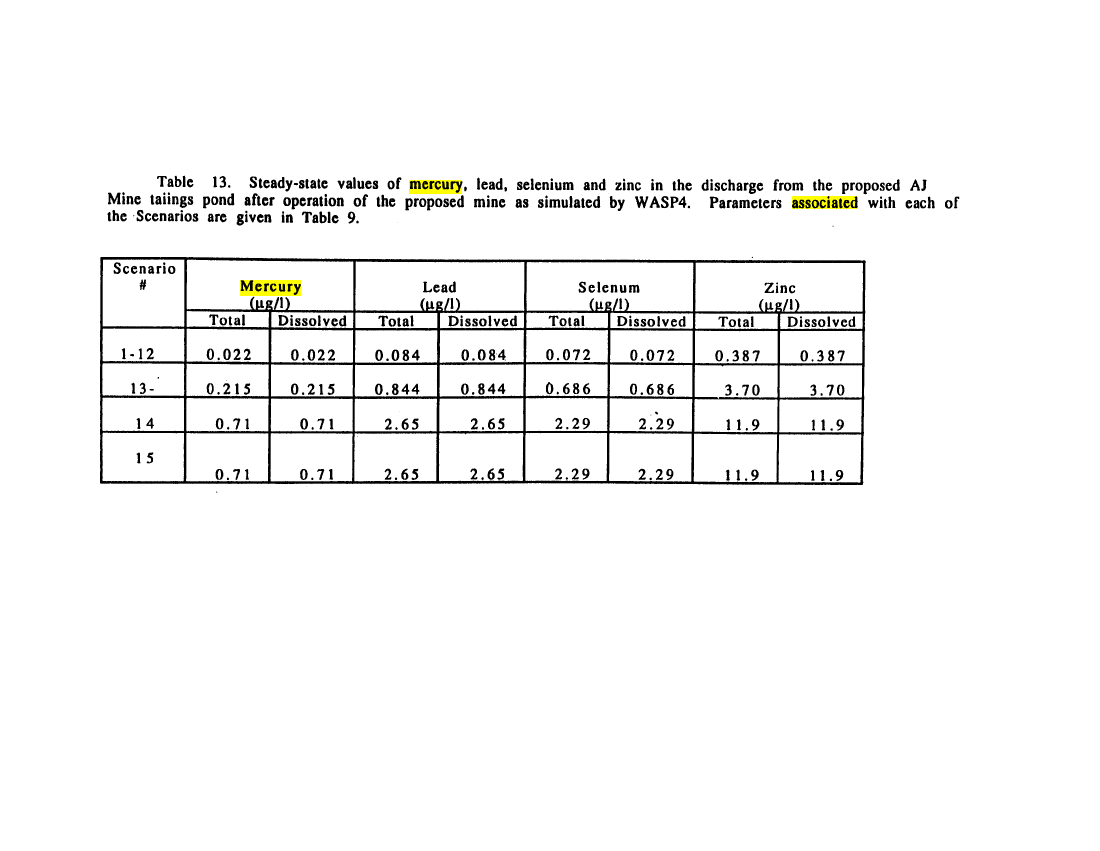
Water Quality Simulation Program (WASP version 4.32) was used to
simulate the levels of solids, cyanide and metals in the water
and sediments of the proposed tailings pond during and after the
operation of the mine.
The WASP software has been thoroughly tested and the program
has been used in a wide variety of applications. The WASP water
quality analysis characterizes the major processes affecting the
distribution of solids, cyanide and certain metals in the
tailings pond. These processes include turbulent mixing in the
pond itself, settling of the tailings, leaching and partitioning
iv
image:
Fifteen of the 42 species of birds documented during formal
censusing are o'f interest to the national program on neotropical
birds (Wilson and. Comet, 1991) . One bird, the marbled murrelet,
whose use of the valley has not been documented, is of concern
because of population declines along the west coast of North
America.
Aquatic resources of the upper portion of Sheep Creek
include a local population of Dolly Vardon char. This population
is isolated from other char populations by .the impassible lower
reach of Sheep Creek.
Gastineau Channel is a north-south oriented channel
separating Douglas Island from the mainland. The shoreline for
approximately 10 miles between Stephens Passage and Juneau is
largely steep sided and rocky. Forty species of demersal fish,
shellfish and other invertebrates have been reported from
Gastineau Channel. Included among these are commercially
"important crab species. The commercial crab fishery was closed
in 1978 but a popular personal use fishery continues (BLM, 1992).
Adequacy of Wastewater Treatment
Chapter VI addresses the projected performance of the
tailings impoundment as a waste treatment system. Water quality
models and information from existing mines are used to determine
whether the discharge from the impoundment, when comingled with
mine drainage, would be likely to meet EPA's New Source
Performance Standards (NSPS) that would apply to the discharge as
end-of-pipe effluent limits. Compliance with Alaska's water
quality standards (WQS) is addressed in Chapter VII.
The chemical composition of the tailings slurry discharge is
discussed. Concentrations of various chemical constituents of
the influent to the tailings pond are presented. They represent
the pollutant loadings to the tailings pond that are subsequently
addressed in water quality models.
Two water quality models were applied to estimate the levels
of pollutants that would be expected in the discharge. The EPA's
Water Quality Simulation Program (WASP version 4.32) was used to
simulate the levels of solids, cyanide and metals in the water
and sediments of the proposed tailings pond during and after the
operation of the mine.
The WASP software has been thoroughly tested and the program
has been used in a wide variety of applications. The WASP water
quality analysis characterizes the major processes affecting the
distribution of solids, cyanide and certain metals in the
tailings pond. These processes include turbulent mixing in the
pond itself, settling of the tailings, leaching and partitioning
iv
image:
 of metals and effects of initial mixing associated with the
discharge.
The WASP model generally reflects the current state of
knowledge for simulation of both inorganic and organic toxic
substances. It was used to predict concentrations of pollutants
in the water column as well as in pore water within the tailings.
During the preparation of this report, however, EPA consulted
with various experts in the field of small particle transport,
some of whom expressed concerns that the WASP4 model might not be
capable of adequately evaluating the effects of the hydrodynamics
of the reservoir on the settling of suspended solids. They
recommended applying the CE-QUAL-W2 water quality model.
EPA therefore simulated the pollutant concentrations in the
tailings impoundment discharge using the CE-QUAL-W2 model
(version 2.04) in order to have a comparison with the earlier
results from the WASP4 model. CE-QUAL-W2 has been applied
successfully to estuarine systems as well as freshwater reservoir
systems. CE-QUAL-W2 generally reflects the current state of
knowledge for simulation of chemical, physical and biological
state variables in estuarine of reservoir systems. While
originally designed to model temperature stratification in Corps
of Engineer managed reservoirs, it has been modified to predict
pollutant concentrations in the water column.
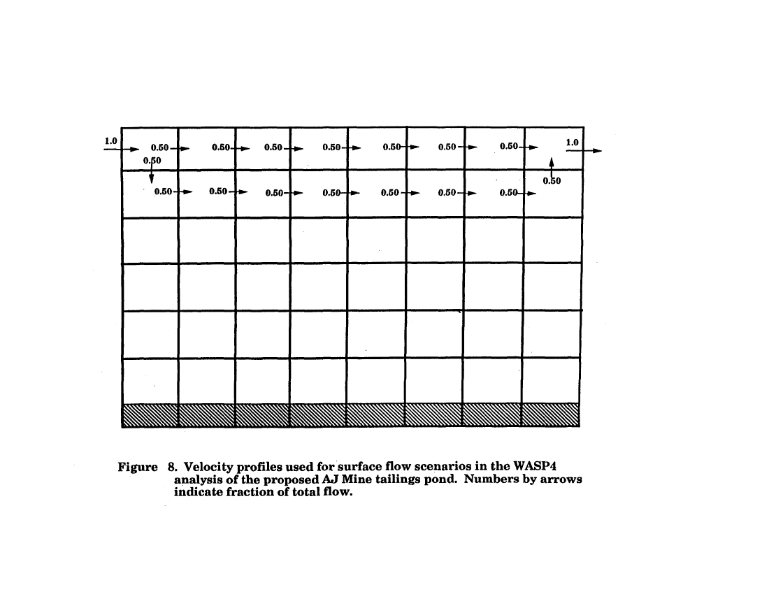
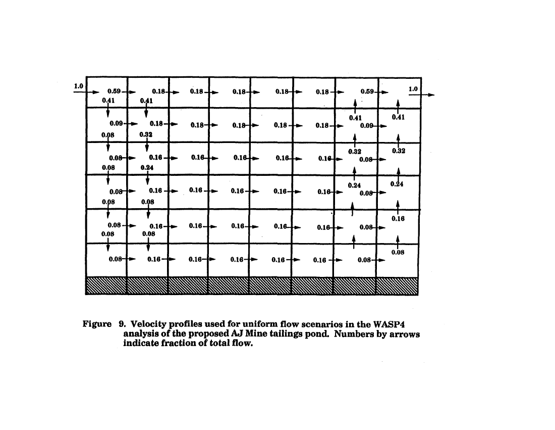
For the WASP4 model analysis, twelve scenarios were
developed that capture the potential variability among such
factors as:
• vertical mixing due to wind stress, kinetic energy
from sources that include Sheep Creek and the waste
stream itself and potential energy associated with
density differences
• hydrodynamic regime
• groundwater inflow
• mixing characteristics of sediment pore water
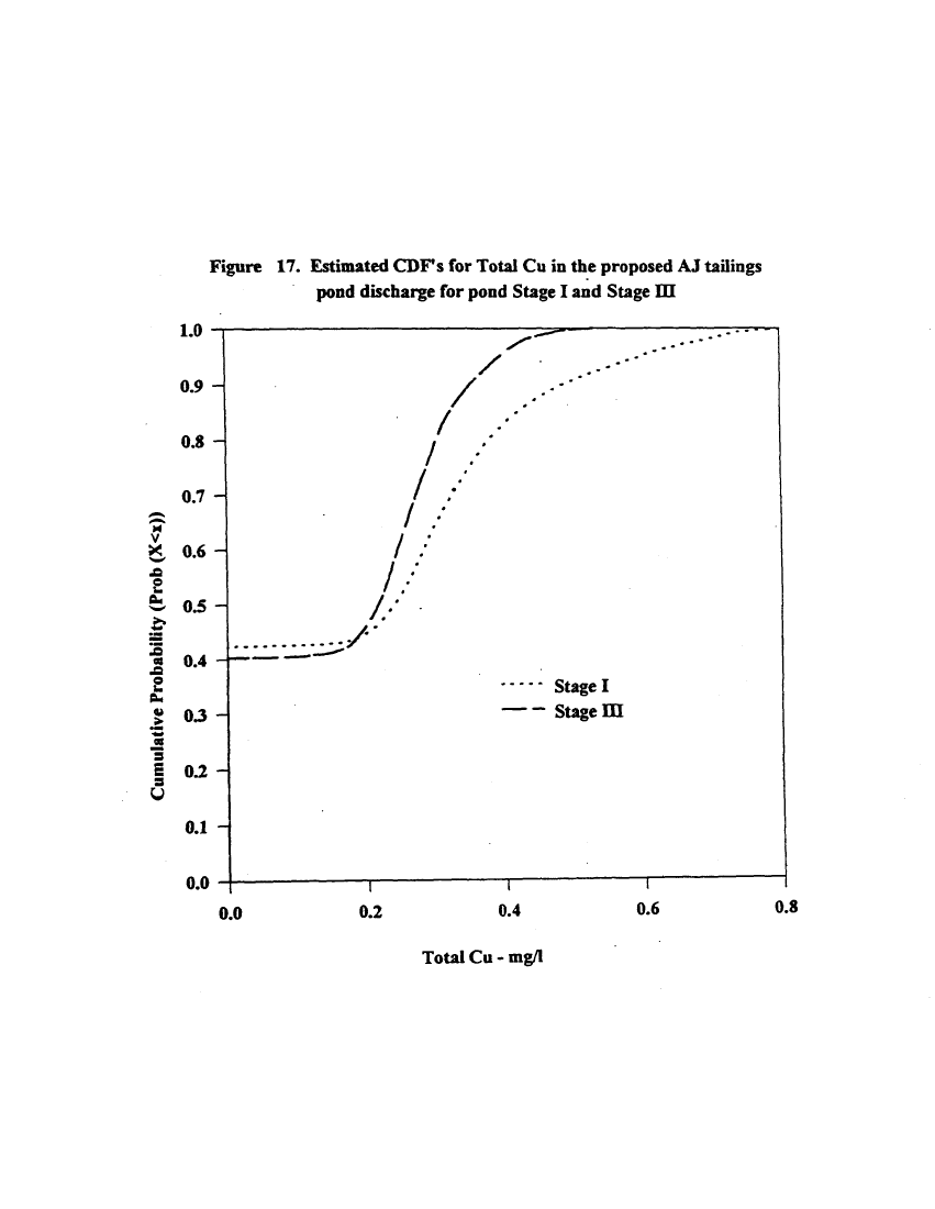
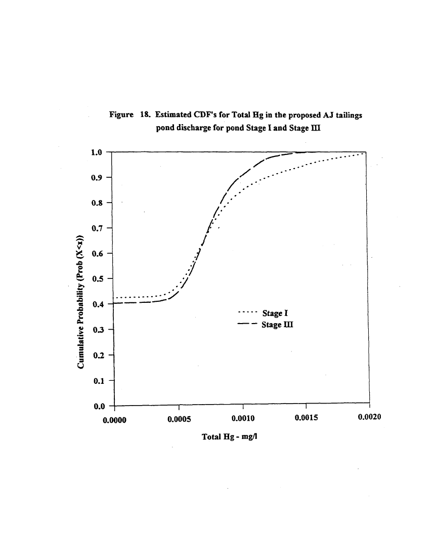
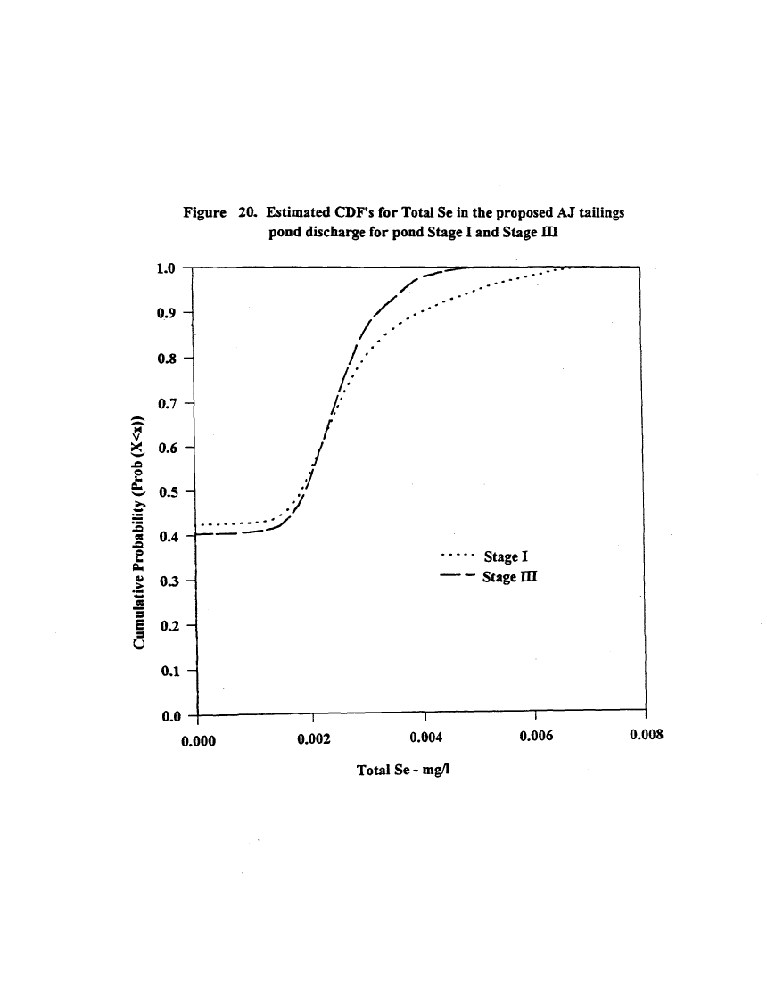
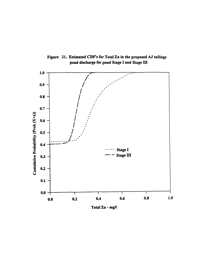
In the CE-QUAL-W2 model analysis, suspended solids and
concentrations of dissolved metals and metals -in suspended solids
in the proposed tailings pond were simulated under the conditions
representing natural variability of weather and inflow hydrology,
as well as estimated variability in the discharge
characteristics. Scenarios that were modeled are based on
different assumptions regarding particle settling rates and
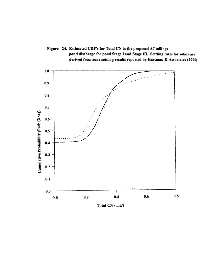
groundwater inflow. Modeling results are presented as cumulative
distribution functions that reflect the probability that each
pollutant in the effluent would exceed a certain concentration.
v
image:
of metals and effects of initial mixing associated with the
discharge.
The WASP model generally reflects the current state of
knowledge for simulation of both inorganic and organic toxic
substances. It was used to predict concentrations of pollutants
in the water column as well as in pore water within the tailings.
During the preparation of this report, however, EPA consulted
with various experts in the field of small particle transport,
some of whom expressed concerns that the WASP4 model might not be
capable of adequately evaluating the effects of the hydrodynamics
of the reservoir on the settling of suspended solids. They
recommended applying the CE-QUAL-W2 water quality model.
EPA therefore simulated the pollutant concentrations in the
tailings impoundment discharge using the CE-QUAL-W2 model
(version 2.04) in order to have a comparison with the earlier
results from the WASP4 model. CE-QUAL-W2 has been applied
successfully to estuarine systems as well as freshwater reservoir
systems. CE-QUAL-W2 generally reflects the current state of
knowledge for simulation of chemical, physical and biological
state variables in estuarine of reservoir systems. While
originally designed to model temperature stratification in Corps
of Engineer managed reservoirs, it has been modified to predict
pollutant concentrations in the water column.
For the WASP4 model analysis, twelve scenarios were
developed that capture the potential variability among such
factors as:
• vertical mixing due to wind stress, kinetic energy
from sources that include Sheep Creek and the waste
stream itself and potential energy associated with
density differences
• hydrodynamic regime
• groundwater inflow
• mixing characteristics of sediment pore water
In the CE-QUAL-W2 model analysis, suspended solids and
concentrations of dissolved metals and metals -in suspended solids
in the proposed tailings pond were simulated under the conditions
representing natural variability of weather and inflow hydrology,
as well as estimated variability in the discharge
characteristics. Scenarios that were modeled are based on
different assumptions regarding particle settling rates and
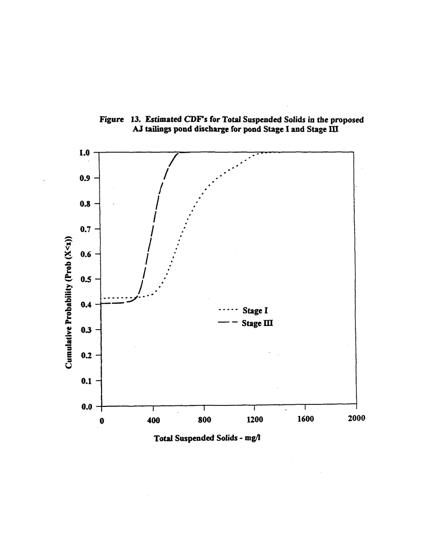
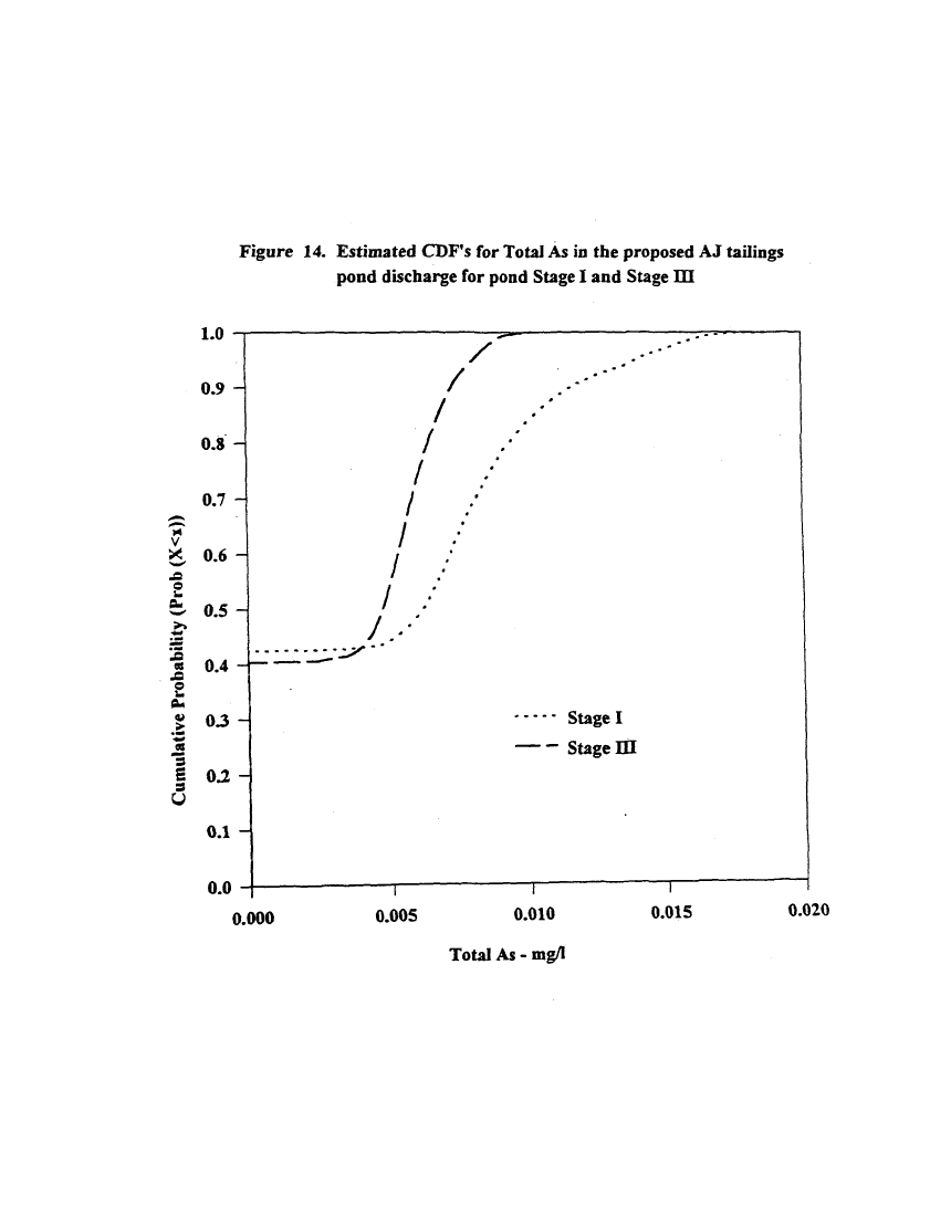
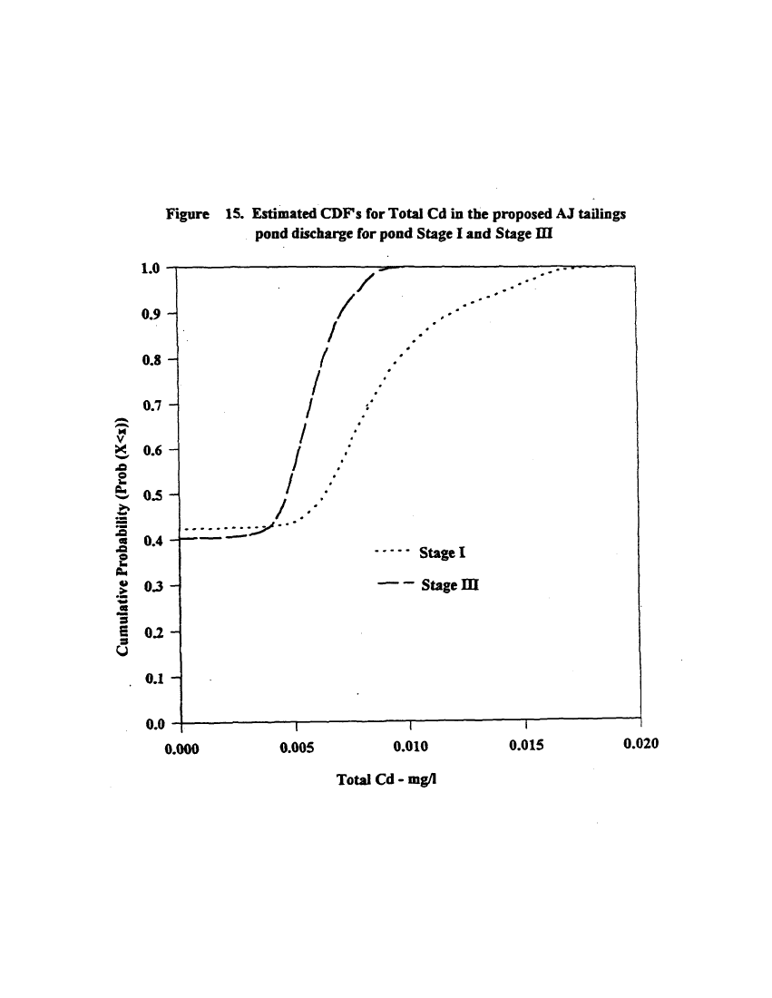
groundwater inflow. Modeling results are presented as cumulative
distribution functions that reflect the probability that each
pollutant in the effluent would exceed a certain concentration.
v
image:
 In additon to water quality modeling, empirical data for
total suspended solids (TSS) from other operating mines were
reviewed for comparison with modeling results. TSS levels for
the mine deemed to be most comparable to the AJ project, Island
Copper, are in the range of results predicted for the AJ
discharge. .
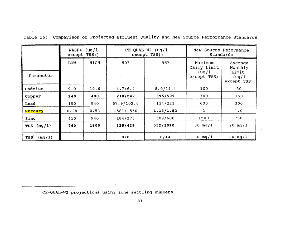
The overall conclusions of the modeling effort are that the
effluent would not meet projected end-of-pipe NSPS for total
suspended solids (TSS) and copper.
Effects on Gastineau Channel
The WASP4 water quality model was also applied to model the
effects of the tailings impoundment discharge on Gastineau
Channel. Chapter VII discusses this effort, which examines both
near-field and far-field (Channel-wide) dilution and dispersion
of the effluent. The central question addressed in this chapter
is whether there is adequate mixing in Gastineau Channel to
dilute the pollutants in the impoundment and mine drainage
effluent to ecologically safe levels in compliance with Alaska's
.WQS.
After a review of previous studies of currents in Gastineau
Channel, the WASP4 model framework is presented. Model runs
include a worst-case discharge scenario and an average case
discharge scenario. The overall conclusion of the analysis is
that WQS would likely be exceeded for cyanide, arsenic and copper
under both average and worst-case scenarios in much of Gastineau
Channel. This is due to the limited flushing within the Channel
and to the ambient background levels of pollutants in the Channel
that limit the Channel's assimilative capacity.
Potential Long-Term Contamination
Chapter VIII describes the impoundment setting and addresses
the type of aquatic habitat that would likely develop in and
around the impoundment. This is followed by an ecological risk
analysis that examines the potential effects of contaminants on
aquatic biota and wildlife likely to inhabit the area.
The impoundment would be an unusual aquatic feature insofar
as it would be a shallow yet steep-sided reservoir. Shallow
lakes generally have gradually sloping shorelines and steep sided
lakes or reservoirs tend to be fairly deep. As such, no
analagous reservoirs or lakes were found in the area upon which
to base a comparison or predict food chains.
With an estimated sedimentation rate of only 1200 cubic
yards per year, coverage of the tailings by sediments to form a
more natural substrate for benthic (bottom dwelling) organisms
would not be expected in the short term. After mine closure,
VI
image:
In additon to water quality modeling, empirical data for
total suspended solids (TSS) from other operating mines were
reviewed for comparison with modeling results. TSS levels for
the mine deemed to be most comparable to the AJ project, Island
Copper, are in the range of results predicted for the AJ
discharge. .
The overall conclusions of the modeling effort are that the
effluent would not meet projected end-of-pipe NSPS for total
suspended solids (TSS) and copper.
Effects on Gastineau Channel
The WASP4 water quality model was also applied to model the
effects of the tailings impoundment discharge on Gastineau
Channel. Chapter VII discusses this effort, which examines both
near-field and far-field (Channel-wide) dilution and dispersion
of the effluent. The central question addressed in this chapter
is whether there is adequate mixing in Gastineau Channel to
dilute the pollutants in the impoundment and mine drainage
effluent to ecologically safe levels in compliance with Alaska's
.WQS.
After a review of previous studies of currents in Gastineau
Channel, the WASP4 model framework is presented. Model runs
include a worst-case discharge scenario and an average case
discharge scenario. The overall conclusion of the analysis is
that WQS would likely be exceeded for cyanide, arsenic and copper
under both average and worst-case scenarios in much of Gastineau
Channel. This is due to the limited flushing within the Channel
and to the ambient background levels of pollutants in the Channel
that limit the Channel's assimilative capacity.
Potential Long-Term Contamination
Chapter VIII describes the impoundment setting and addresses
the type of aquatic habitat that would likely develop in and
around the impoundment. This is followed by an ecological risk
analysis that examines the potential effects of contaminants on
aquatic biota and wildlife likely to inhabit the area.
The impoundment would be an unusual aquatic feature insofar
as it would be a shallow yet steep-sided reservoir. Shallow
lakes generally have gradually sloping shorelines and steep sided
lakes or reservoirs tend to be fairly deep. As such, no
analagous reservoirs or lakes were found in the area upon which
to base a comparison or predict food chains.
With an estimated sedimentation rate of only 1200 cubic
yards per year, coverage of the tailings by sediments to form a
more natural substrate for benthic (bottom dwelling) organisms
would not be expected in the short term. After mine closure,
VI
image:
 fish populations would not be likely without a managed food base.
Insect production and transport by the inflowing small streams
would not provide enough food to sustain fish. In addition, the
impoundment lacks the habitat characteristics required for
species survival (e.g., cover and spawning areas). Construction
of the upstream diversion dam would impede fish access to
potential spawning areas above the impoundment.
The post-closure vegetation expected on the surrounding
slopes, and avalanche dissipators is likely to be alder and
shrubs. It has been suggested that the impoundment's shoreline
would create new wetland habitats, however, this has not been
analyzed in any detail and, given the steep surrounding terrain,
seems unlikely.
An. ecological risk assessment evaluated the potential
toxicity of contaminant concentrations in pore water (i.e., water
trapped between tailings particles where bottom dwelling plants
and animals would root or burrow) , sediments, and the water
column. In addition, three species were selected for an analysis
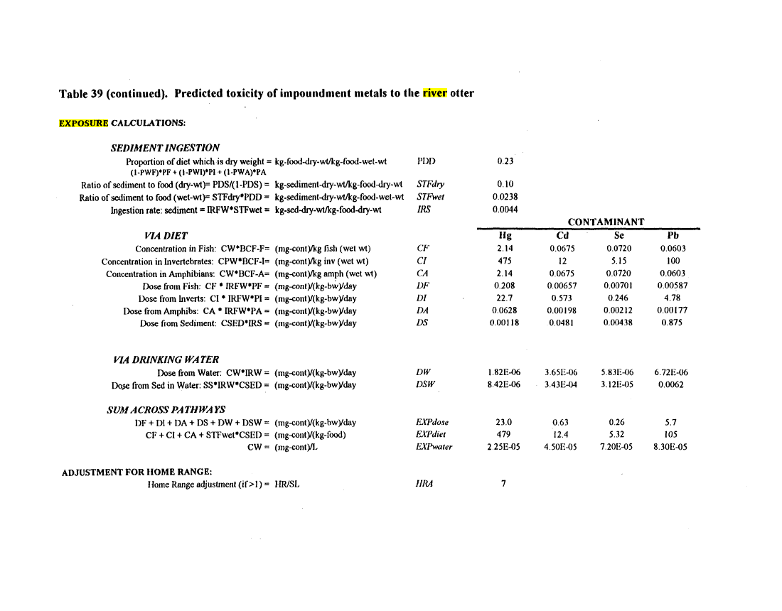
of the effects of the heavy metals in the tailings on wildlife.
The kingfisher, spotted sandpiper and river otter were evaluated
based on the likelihood that they would inhabit the impoundment
area and would ingest water, organisms that would bioaccumulate
the metals, as well as the tailings themselves.
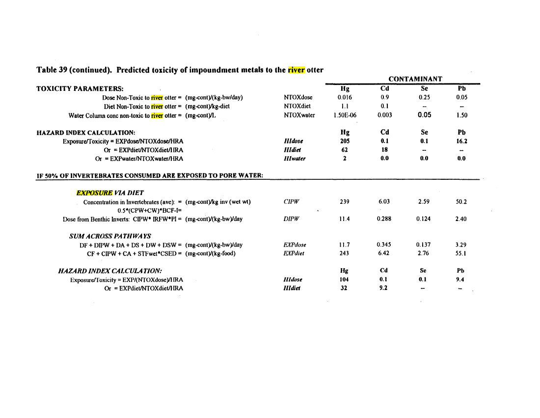
The results of this analysis indicate that aquatic biota
(including wildlife) would be at substantial risk from the
contaminants in the tailings. 'Water quality criteria would
likely be exceeded at high levels in the pore water (up to 200
times the acute criterion for cyanide) and water column (2 times
the acute criterion for copper); sediment concentrations would
likely exceed benchmark comparison values (over 400 times the
lowest effect level for cyanide); and wildlife are likely to be
at substantial risk from their exposure to high levels of metals
in their diets (exceeding draft Great Lakes criterion for mercury
by over 200 times),
Canadian studies of lakes used for disposal of mine tailings
were also reviewed. These studies examined to some degree the
impacts of mine tailings disposal on the health of the aquatic
systems in these lakes. The findings of these studies, however,
do not alter EPA's conclusion that the Sheep Creek tailings
impoundment would present substantial risks to wildlife in the
long-term.
Mitigating Water Quality Impacts
In view of the findings of the two previous chapters, which
conclude that the project as proposed would, likely violate
effluent limits during operation and, after closure, place
wildlife at substantial risk, Chapter IX addresses potential
vii
image:
fish populations would not be likely without a managed food base.
Insect production and transport by the inflowing small streams
would not provide enough food to sustain fish. In addition, the
impoundment lacks the habitat characteristics required for
species survival (e.g., cover and spawning areas). Construction
of the upstream diversion dam would impede fish access to
potential spawning areas above the impoundment.
The post-closure vegetation expected on the surrounding
slopes, and avalanche dissipators is likely to be alder and
shrubs. It has been suggested that the impoundment's shoreline
would create new wetland habitats, however, this has not been
analyzed in any detail and, given the steep surrounding terrain,
seems unlikely.
An. ecological risk assessment evaluated the potential
toxicity of contaminant concentrations in pore water (i.e., water
trapped between tailings particles where bottom dwelling plants
and animals would root or burrow) , sediments, and the water
column. In addition, three species were selected for an analysis
of the effects of the heavy metals in the tailings on wildlife.
The kingfisher, spotted sandpiper and river otter were evaluated
based on the likelihood that they would inhabit the impoundment
area and would ingest water, organisms that would bioaccumulate
the metals, as well as the tailings themselves.
The results of this analysis indicate that aquatic biota
(including wildlife) would be at substantial risk from the
contaminants in the tailings. 'Water quality criteria would
likely be exceeded at high levels in the pore water (up to 200
times the acute criterion for cyanide) and water column (2 times
the acute criterion for copper); sediment concentrations would
likely exceed benchmark comparison values (over 400 times the
lowest effect level for cyanide); and wildlife are likely to be
at substantial risk from their exposure to high levels of metals
in their diets (exceeding draft Great Lakes criterion for mercury
by over 200 times),
Canadian studies of lakes used for disposal of mine tailings
were also reviewed. These studies examined to some degree the
impacts of mine tailings disposal on the health of the aquatic
systems in these lakes. The findings of these studies, however,
do not alter EPA's conclusion that the Sheep Creek tailings
impoundment would present substantial risks to wildlife in the
long-term.
Mitigating Water Quality Impacts
In view of the findings of the two previous chapters, which
conclude that the project as proposed would, likely violate
effluent limits during operation and, after closure, place
wildlife at substantial risk, Chapter IX addresses potential
vii
image:
 measures for reducing water quality impacts to significantly
lower levels. "Measures that are addressed, include secondary
treatment of the effluent, measures for reducing total suspended
solids, eliminating the cyanide leach circuit and potential means
for isolating the tailings to minimize the risk of long-term
contamination. The Powerline/Icy Gulch tailings disposal
alternative is briefly reviewed with respect to its potential
feasibility as a disposal site using a more conventional, sub-
aerial tailings disposal method (i.e., tailings would not be
discharged underwater), surface water diversion and conventional
reclamation (tailings covered with soil rather than water).
No single measure or combination of measures are deemed to
be adequate to reduce both short-term (during operation) and
long-term (post-operation) water quality impacts to significantly
lower levels that would clearly avoid significant degradation of
waters of the U.S. If feasible, the Powerline/Icy Gulch
alternative (with subaerial tailings deposition, surface water
diversion, secondary wastewater treatment and conventional
reclamation) would offer some significant advantages relative to
the Sheep Creek alternative in terms of minimizing degradation of
waters of the U.S. The feasibility of this alternative, as well
as other potential measures such as elimination of the cyanide
leach circuit, would require much more in depth evaluation by
Echo Bay and resource agencies.
Mitigating Ecological impacts
Chapter X addresses options for mitigating or off-setting
the loss of aquatic habitats (wetlands and Sheep Creek) that
would occur if the tailings impoundment was constructed as
proposed. Due to the findings of Chapter VIII, i.e., that risks
to wildlife from exposure to heavy metals would be high, the
creation of the impoundment itself is not considered to in any
way offset the loss of Sheep Creek and the wetlands of Sheep
Creek Valley. These wetlands are part of a diverse mosaic of
plant communities that support a diversity and abundance of birds
and other wildlife. The wetlands and Sheep Creek itself
contribute to the overall aesthetic value of the area which is a
popular hiking destination.
Options examined for off-setting the loss of aquatic
habitats include restoration of Lemon Creek Valley, enhancing
three ponds in the Juneau area and performing certain habitat and
recreational improvements at the U.S. Forest Service Mendenhall
Glacier Visitor's Center.
All of these options have serious limitations and none are
deemed capable of off-setting the unique values of Sheep Creek
and the wetlands of Sheep Creek Valley, particularly the
significant loss of high quality migratory bird habitat.
Vlll
image:
measures for reducing water quality impacts to significantly
lower levels. "Measures that are addressed, include secondary
treatment of the effluent, measures for reducing total suspended
solids, eliminating the cyanide leach circuit and potential means
for isolating the tailings to minimize the risk of long-term
contamination. The Powerline/Icy Gulch tailings disposal
alternative is briefly reviewed with respect to its potential
feasibility as a disposal site using a more conventional, sub-
aerial tailings disposal method (i.e., tailings would not be
discharged underwater), surface water diversion and conventional
reclamation (tailings covered with soil rather than water).
No single measure or combination of measures are deemed to
be adequate to reduce both short-term (during operation) and
long-term (post-operation) water quality impacts to significantly
lower levels that would clearly avoid significant degradation of
waters of the U.S. If feasible, the Powerline/Icy Gulch
alternative (with subaerial tailings deposition, surface water
diversion, secondary wastewater treatment and conventional
reclamation) would offer some significant advantages relative to
the Sheep Creek alternative in terms of minimizing degradation of
waters of the U.S. The feasibility of this alternative, as well
as other potential measures such as elimination of the cyanide
leach circuit, would require much more in depth evaluation by
Echo Bay and resource agencies.
Mitigating Ecological impacts
Chapter X addresses options for mitigating or off-setting
the loss of aquatic habitats (wetlands and Sheep Creek) that
would occur if the tailings impoundment was constructed as
proposed. Due to the findings of Chapter VIII, i.e., that risks
to wildlife from exposure to heavy metals would be high, the
creation of the impoundment itself is not considered to in any
way offset the loss of Sheep Creek and the wetlands of Sheep
Creek Valley. These wetlands are part of a diverse mosaic of
plant communities that support a diversity and abundance of birds
and other wildlife. The wetlands and Sheep Creek itself
contribute to the overall aesthetic value of the area which is a
popular hiking destination.
Options examined for off-setting the loss of aquatic
habitats include restoration of Lemon Creek Valley, enhancing
three ponds in the Juneau area and performing certain habitat and
recreational improvements at the U.S. Forest Service Mendenhall
Glacier Visitor's Center.
All of these options have serious limitations and none are
deemed capable of off-setting the unique values of Sheep Creek
and the wetlands of Sheep Creek Valley, particularly the
significant loss of high quality migratory bird habitat.
Vlll
image:
 Conclusions
Based on the findings of this report, EPA concludes that
there is a high potential for significant degradation of waters
of the U.S. both within Gastineau Channel and within the tailings
impoundment after closure, i.e., after it is no longer used for
treatment of wastewater and disposal of mine tailings. The
specific major findings that lead to this conclusion are as
follows:
Finding #1:
During operation, the wastewater discharge from the
impoundment co-mingled with mine drainage is likely to
exceed EPA's New Source Performance Standards (end-of-pipe
effluent limits) for total suspended solids, copper and
possibly mercury (see Chapter VI)..
Finding #2:
During operation, the wastewater discharge is likely to
cause widespread exceedances of state of Alaska water
quality standards for cyanide, arsenic, copper and possibly
mercury and lead (see Chapter VII);
Finding #3:
After closure, indigenous wildlife that would likely inhabit
the tailings impoundment would be at substantial risk due to
contaminants that would likely persist in the impoundment.
Water quality criteria would likely be exceeded at high
levels in the pore water (up to 200 times the acute
criterion for cyanide) and water column (2 times the acute
criterion for copper); sediment concentrations would exceed
benchmark comparison values (over 400 times the lowest
effect level for cyanide); and wildlife are likely to be at
substantial risk from their exposure to high levels of
metals in their diets (exceeding draft Great Lakes criterion
for mercury by over 200 times; see Chapter VIII).
Finding #4:
Unlike the Kensington Mine project, reliable measures (e.g.,
secondary treatment of the effluent, isolating the tailings)
for reducing the anticipated water quality impacts described
above to significantly lower levels do not appear to be
feasible. Others, such as eliminating the cyanide leaching
process or using subaerial tailings deposition and
conventional reclamation at an alternative disposal site,
would require much more detailed analysis to determine
feasibility as well as overall environmental impacts (see
Chapter IX).
IX
image:
Conclusions
Based on the findings of this report, EPA concludes that
there is a high potential for significant degradation of waters
of the U.S. both within Gastineau Channel and within the tailings
impoundment after closure, i.e., after it is no longer used for
treatment of wastewater and disposal of mine tailings. The
specific major findings that lead to this conclusion are as
follows:
Finding #1:
During operation, the wastewater discharge from the
impoundment co-mingled with mine drainage is likely to
exceed EPA's New Source Performance Standards (end-of-pipe
effluent limits) for total suspended solids, copper and
possibly mercury (see Chapter VI)..
Finding #2:
During operation, the wastewater discharge is likely to
cause widespread exceedances of state of Alaska water
quality standards for cyanide, arsenic, copper and possibly
mercury and lead (see Chapter VII);
Finding #3:
After closure, indigenous wildlife that would likely inhabit
the tailings impoundment would be at substantial risk due to
contaminants that would likely persist in the impoundment.
Water quality criteria would likely be exceeded at high
levels in the pore water (up to 200 times the acute
criterion for cyanide) and water column (2 times the acute
criterion for copper); sediment concentrations would exceed
benchmark comparison values (over 400 times the lowest
effect level for cyanide); and wildlife are likely to be at
substantial risk from their exposure to high levels of
metals in their diets (exceeding draft Great Lakes criterion
for mercury by over 200 times; see Chapter VIII).
Finding #4:
Unlike the Kensington Mine project, reliable measures (e.g.,
secondary treatment of the effluent, isolating the tailings)
for reducing the anticipated water quality impacts described
above to significantly lower levels do not appear to be
feasible. Others, such as eliminating the cyanide leaching
process or using subaerial tailings deposition and
conventional reclamation at an alternative disposal site,
would require much more detailed analysis to determine
feasibility as well as overall environmental impacts (see
Chapter IX).
IX
image:
 Finding #5;
The loss of aquatic habitat (Sheep Creek and associated
wetlands) would be significant due to their contribution to
the unique diversity and productivity within the Juneau
area, particularly in terms of migratory bird habitat and
the aesthetic quality and recreational value of Sheep Creek
valley. Potential measures .identified to replace these
values, including on-site and off-site measures,, do not
appear either feasible or adequate to prevent a significant
loss of aquatic resources (see Chapter X).
image:
Finding #5;
The loss of aquatic habitat (Sheep Creek and associated
wetlands) would be significant due to their contribution to
the unique diversity and productivity within the Juneau
area, particularly in terms of migratory bird habitat and
the aesthetic quality and recreational value of Sheep Creek
valley. Potential measures .identified to replace these
values, including on-site and off-site measures,, do not
appear either feasible or adequate to prevent a significant
loss of aquatic resources (see Chapter X).
image:
 I. INTRODUCTION
The Alaska Juneau (A3) Gold Mine project is a proposal by
Echo Bay Alaska (Echo Bay) to reopen the historic AJ mine near
Juneau in southeast Alaska (see figure 1). The proposal entails
mining approximately 22,500 tons of ore per day and, after
crushing and grinding the ore, recovering gold through the froth
flotation and carbon-in-leach (CIL; also referred to as cyanide
leach) processes. After destruction of residual cyanide in the
CIL tailings using a sulfur dioxide/air process, the tailings
•would then be discharged in a slurry form to a tailings
impoundment that would be constructed in the sheep Creek Valley.
Mine drainage water and process water, equivalent in volume to
the net precipitation (after evaporation) over the impoundment,
would be discharged to Gastineau Channel, approximately one mile
to the west of the tailings impoundment (see Figure 2) .
This report evaluates short and long-term water quality
impacts from the project as well as long-term ecological
consequences. Findings and recommendations have been developed
to assist the Alaska District Corps of Engineers in determining
whether the proposed project complies with the Clean Water Act
(CWA) Section 404(to)(1) Guidelines. A CWA Section 404 permit is
required to place fill for construction of the tailings
impoundment which is intended to function as a wastewater
treatment system. These permits are issued by the Corps of
Engineers with the assistance of EPA.
If permitted under CWA section 404, the impoundment would
not be considered a jurisdictional water of the U.S. As such, a
permit to discharge process wastewater, which includes tailings,
into the impoundment would not be required but a CWA section 402
permit would be required for the discharge from the impoundment
to Gastineau Channel. CWA section 402 permits are subject to the
provisions of the National Pollutant Discharge Elimination System
(NPDES) administered by EPA. The state of Alaska can require
more stringent conditions if necessary to meet state water
quality standards, in accordance with Section 401 of the Clean
Water Act.
In summary, this report addresses the overall question of
whether this project can be constructed and operated so as to
comply with certain critical provisions of both CWA sections 404
and 402. These two permits are closely related. The primary
purpose for the 404 permit, other than for permanent tailings
disposal, is to construct a tailings impoundment wastewater
treatment system that would ensure that discharges from the
impoundment would meet the provisions of the CWA section 402
permit. Therefore a 404 permit should only be issued if it can
be demonstrated that there is reasonable assurance that the 402
permit provisions would be attained.
image:
I. INTRODUCTION
The Alaska Juneau (A3) Gold Mine project is a proposal by
Echo Bay Alaska (Echo Bay) to reopen the historic AJ mine near
Juneau in southeast Alaska (see figure 1). The proposal entails
mining approximately 22,500 tons of ore per day and, after
crushing and grinding the ore, recovering gold through the froth
flotation and carbon-in-leach (CIL; also referred to as cyanide
leach) processes. After destruction of residual cyanide in the
CIL tailings using a sulfur dioxide/air process, the tailings
•would then be discharged in a slurry form to a tailings
impoundment that would be constructed in the sheep Creek Valley.
Mine drainage water and process water, equivalent in volume to
the net precipitation (after evaporation) over the impoundment,
would be discharged to Gastineau Channel, approximately one mile
to the west of the tailings impoundment (see Figure 2) .
This report evaluates short and long-term water quality
impacts from the project as well as long-term ecological
consequences. Findings and recommendations have been developed
to assist the Alaska District Corps of Engineers in determining
whether the proposed project complies with the Clean Water Act
(CWA) Section 404(to)(1) Guidelines. A CWA Section 404 permit is
required to place fill for construction of the tailings
impoundment which is intended to function as a wastewater
treatment system. These permits are issued by the Corps of
Engineers with the assistance of EPA.
If permitted under CWA section 404, the impoundment would
not be considered a jurisdictional water of the U.S. As such, a
permit to discharge process wastewater, which includes tailings,
into the impoundment would not be required but a CWA section 402
permit would be required for the discharge from the impoundment
to Gastineau Channel. CWA section 402 permits are subject to the
provisions of the National Pollutant Discharge Elimination System
(NPDES) administered by EPA. The state of Alaska can require
more stringent conditions if necessary to meet state water
quality standards, in accordance with Section 401 of the Clean
Water Act.
In summary, this report addresses the overall question of
whether this project can be constructed and operated so as to
comply with certain critical provisions of both CWA sections 404
and 402. These two permits are closely related. The primary
purpose for the 404 permit, other than for permanent tailings
disposal, is to construct a tailings impoundment wastewater
treatment system that would ensure that discharges from the
impoundment would meet the provisions of the CWA section 402
permit. Therefore a 404 permit should only be issued if it can
be demonstrated that there is reasonable assurance that the 402
permit provisions would be attained.
image:
 City and
Borough of
Juneau
e
..«V4L ±
L,
City and Borough
Figure 1
Location Map
J
image:
City and
Borough of
Juneau
e
..«V4L ±
L,
City and Borough
Figure 1
Location Map
J
image:
 2000 COO
7000 FCCT
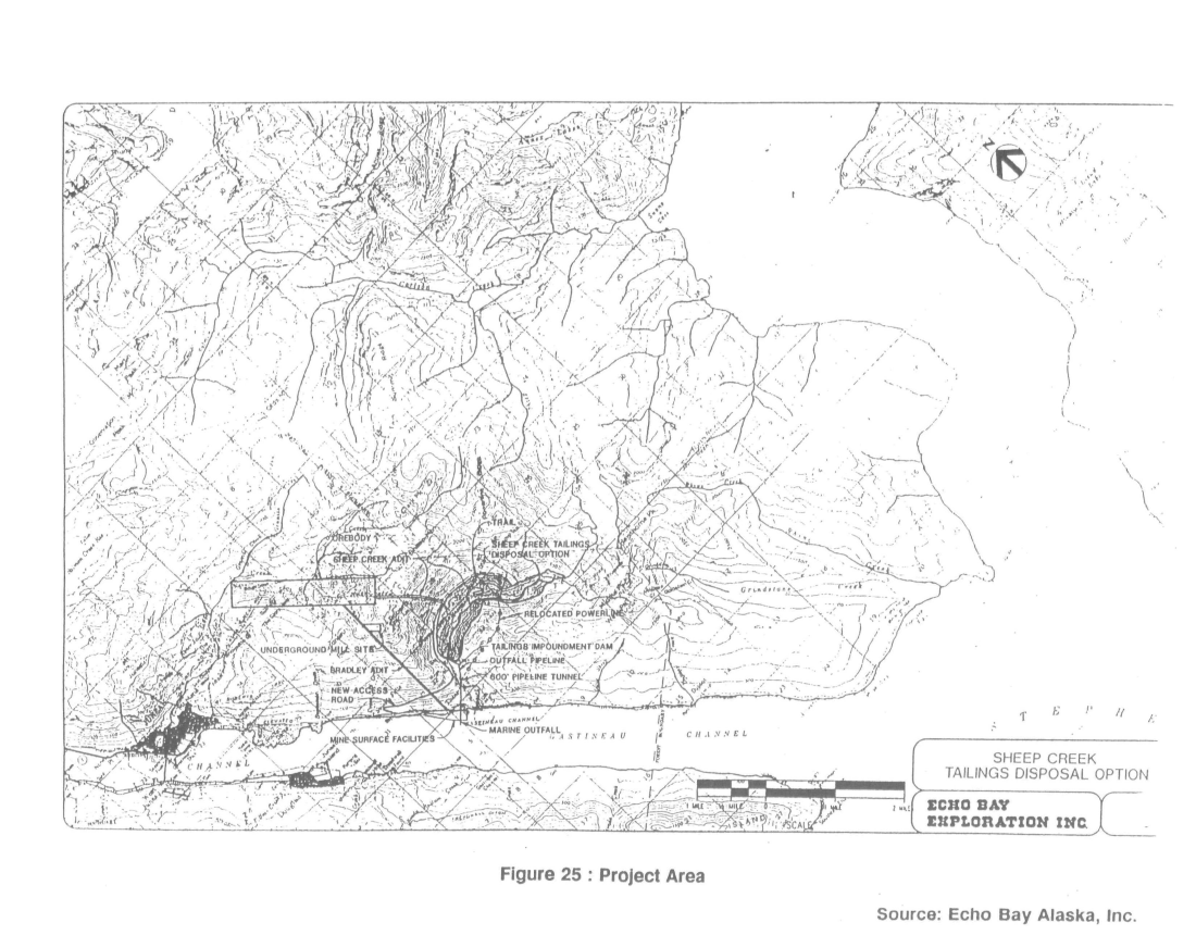
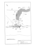
Figure 2
A-J Mine Project
Proposed Tailings Impoundment
Sheep Creek
Source: A-J Mine Project FEIS. BLM, 1992
image:
2000 COO
7000 FCCT
Figure 2
A-J Mine Project
Proposed Tailings Impoundment
Sheep Creek
Source: A-J Mine Project FEIS. BLM, 1992
image:
 II. SCOPE OF REPORT
This report addresses impacts from the proposed discharge of
process wastes, both solid and liquid, from the AJ mine project.
These impacts are analyzed with respect to risks associated with
the potential release of contaminants into the aquatic
environment and with respect to losses of aquatic habitat
productivity (e.g., wetlands) from direct physical disturbance.
A fundamental question which this report addresses is whether or
not there is a reasonable assurance that the impoundment would in
fact provide adequate treatment such that EPA's New Source
Performance Standards (NSPS; see 40 CFR 440.104) would be met at
the point of discharge to Gastineau Channel and that State of
Alaska water quality standards (WQS) would be met in the
receiving waters. Chapter VI addresses this question, relying
heavily on water quality modeling analyses. Chapter VII
addresses overall water quality impacts to Gastineau Channel..
Another fundamental question relates to whether there is
reasonable assurance that the proposed method for tailings
disposal and long-term maintenance would prevent release of
contaminants in harmful quantities. Chapter VIII presents an
ecological risk assessment of post-operation conditions and
reviews studies of Canadian lakes that have been used for
tailings disposal.
In view of the findings of the chapters VI, VII AND VIII,
the report addresses potential measures for mitigating or
reducing water quality impacts to significantly lower levels in
Chapter IX.
A third key question is whether the significant impacts
caused by construction and operation of the tailings impoundment
can- be mitigated to the point that overall impacts on aquatic
resources are acceptable. Optional mitigation plans and
strategies are reviewed in Chapter X.
This report addresses the AJ mine project design reflected
in the CWA §404 permit application and in the Final Environmental
Impact Statement prepared by the Bureau of Land Management. The
only significant project modification which is not considered in
the 404 application or FEIS but which is addressed in this report
is a proposal by Echo Bay to construct a diversion dam at the
headwaters of Sheep Creek Valley. According to Echo Bay, (EBA,
3/17/1994) this dam would allow diversion of approximately one-
third of the flow on Sheep Creek through a pipeline that would
float on the surface of the reservoir and then discharge to lower
Sheep Creek (see Appendix E).
The information and analyses upon which this report is
largely based were developed by Echo Bay and their consultants
and the Bureau of Land Management and their third party
image:
II. SCOPE OF REPORT
This report addresses impacts from the proposed discharge of
process wastes, both solid and liquid, from the AJ mine project.
These impacts are analyzed with respect to risks associated with
the potential release of contaminants into the aquatic
environment and with respect to losses of aquatic habitat
productivity (e.g., wetlands) from direct physical disturbance.
A fundamental question which this report addresses is whether or
not there is a reasonable assurance that the impoundment would in
fact provide adequate treatment such that EPA's New Source
Performance Standards (NSPS; see 40 CFR 440.104) would be met at
the point of discharge to Gastineau Channel and that State of
Alaska water quality standards (WQS) would be met in the
receiving waters. Chapter VI addresses this question, relying
heavily on water quality modeling analyses. Chapter VII
addresses overall water quality impacts to Gastineau Channel..
Another fundamental question relates to whether there is
reasonable assurance that the proposed method for tailings
disposal and long-term maintenance would prevent release of
contaminants in harmful quantities. Chapter VIII presents an
ecological risk assessment of post-operation conditions and
reviews studies of Canadian lakes that have been used for
tailings disposal.
In view of the findings of the chapters VI, VII AND VIII,
the report addresses potential measures for mitigating or
reducing water quality impacts to significantly lower levels in
Chapter IX.
A third key question is whether the significant impacts
caused by construction and operation of the tailings impoundment
can- be mitigated to the point that overall impacts on aquatic
resources are acceptable. Optional mitigation plans and
strategies are reviewed in Chapter X.
This report addresses the AJ mine project design reflected
in the CWA §404 permit application and in the Final Environmental
Impact Statement prepared by the Bureau of Land Management. The
only significant project modification which is not considered in
the 404 application or FEIS but which is addressed in this report
is a proposal by Echo Bay to construct a diversion dam at the
headwaters of Sheep Creek Valley. According to Echo Bay, (EBA,
3/17/1994) this dam would allow diversion of approximately one-
third of the flow on Sheep Creek through a pipeline that would
float on the surface of the reservoir and then discharge to lower
Sheep Creek (see Appendix E).
The information and analyses upon which this report is
largely based were developed by Echo Bay and their consultants
and the Bureau of Land Management and their third party
image:
 contractor during the Environmental Impact Statement (EIS)
process. Our analysis entailed a review of the Echo Bay
submittals and EIS findings for completeness and technical
validity, as well as a review of the available relevant technical
literature. Much of the analysis is devoted to examining
reasonably foreseeable "worst case" situations that could arise
during the life of the project. Demonstrating that the project
would meet environmental standards during extreme conditions is
critical to determining whether there is reasonable assurance
that such standards can be met at all times.
Additional information provided by Echo Bay in response to
EPA concerns raised during the development of this report has
also been relied upon. All of the above information is a part of
the administrative record and is available for review at EPA's
Region 10 Office in Seattle.
image:
contractor during the Environmental Impact Statement (EIS)
process. Our analysis entailed a review of the Echo Bay
submittals and EIS findings for completeness and technical
validity, as well as a review of the available relevant technical
literature. Much of the analysis is devoted to examining
reasonably foreseeable "worst case" situations that could arise
during the life of the project. Demonstrating that the project
would meet environmental standards during extreme conditions is
critical to determining whether there is reasonable assurance
that such standards can be met at all times.
Additional information provided by Echo Bay in response to
EPA concerns raised during the development of this report has
also been relied upon. All of the above information is a part of
the administrative record and is available for review at EPA's
Region 10 Office in Seattle.
image:
 III. POLICY BACKGROUND
On October 2, 1992, EPA's Assistant Administrator for Water
wrote a memorandum to Region 10's Water Division Director
requesting that the Region provide technical assistance to the
Corps of Engineers with respect to pending CWA §404 permits for
the AJ and Kensington gold mine projects (see Appendix A). The
EPA and the Corps of Engineers agreed, as reflected in this memo,
that if the impoundments created by the discharge of fill
material contemplated as part of the Kensington and AJ gold mine
projects are each permitted under an individual CWA §404 permit
for purposes of creating waste treatment systems, they would not
be considered waters of the U.S. They would be considered non-
jurisdictional waste treatment systems which, by definition (see
40 CFR 122.2 in Appendix A), are not waters of the U.S.
The October 2, 1992, memo reflects an agreement between EPA
and the Corps concerning the respective roles of CWA §402 and CWA
§404 permits for the mine tailings ponds at the AJ and Kensington
projects. A CWA §402 permit, which EPA would issue, is a
wastewater discharge permit under EPA's National Pollutant
Discharge Elimination System (NPDES) program. It is required for
wastewater discharges from the tailings impoundments. A CWA §404
permit, which the Corps would issue, is required to place fill
material (the dams) to construct the tailings impoundments.
Under the agreement, the CWA §404 permit evaluation must address
the effects not only of placing fill for the dam but also the
effects of the entire impoundment, including its use as a waste
treatment system, on waters of the U.S. Since the purpose of
creating the impoundment is to establish a waste treatment
system, EPA agreed to provide technical assistance to the Corps
with respect to water quality and mitigation as well as overall
compliance with the CWA §404(b)(1) Guidelines. This Technical
Assistance Report (TAR) is part of EPA's assistance in that
regard.
The §404(b)(l) Guidelines (see Appendix A) promulgated by
EPA are the substantive regulations that must be satisfied before
a §404 permit can be issued. In accordance with current Region
10 policy, the Region will consider the following factors with
respect to compliance with the §404(b)(l) Guidelines:
1) The proposed treatment system is determined by the
Corps of Engineers and EPA to be the least
environmentally damaging practicable alternative for
meeting the applicant's project purpose of treating
wastewater in order to meet all applicable federal,
state and local wastewater discharge limits [see 40 CFR
230.10 (a)];
2) The proposed project does not cause or contribute to
any violations of state water quality standards
image:
III. POLICY BACKGROUND
On October 2, 1992, EPA's Assistant Administrator for Water
wrote a memorandum to Region 10's Water Division Director
requesting that the Region provide technical assistance to the
Corps of Engineers with respect to pending CWA §404 permits for
the AJ and Kensington gold mine projects (see Appendix A). The
EPA and the Corps of Engineers agreed, as reflected in this memo,
that if the impoundments created by the discharge of fill
material contemplated as part of the Kensington and AJ gold mine
projects are each permitted under an individual CWA §404 permit
for purposes of creating waste treatment systems, they would not
be considered waters of the U.S. They would be considered non-
jurisdictional waste treatment systems which, by definition (see
40 CFR 122.2 in Appendix A), are not waters of the U.S.
The October 2, 1992, memo reflects an agreement between EPA
and the Corps concerning the respective roles of CWA §402 and CWA
§404 permits for the mine tailings ponds at the AJ and Kensington
projects. A CWA §402 permit, which EPA would issue, is a
wastewater discharge permit under EPA's National Pollutant
Discharge Elimination System (NPDES) program. It is required for
wastewater discharges from the tailings impoundments. A CWA §404
permit, which the Corps would issue, is required to place fill
material (the dams) to construct the tailings impoundments.
Under the agreement, the CWA §404 permit evaluation must address
the effects not only of placing fill for the dam but also the
effects of the entire impoundment, including its use as a waste
treatment system, on waters of the U.S. Since the purpose of
creating the impoundment is to establish a waste treatment
system, EPA agreed to provide technical assistance to the Corps
with respect to water quality and mitigation as well as overall
compliance with the CWA §404(b)(1) Guidelines. This Technical
Assistance Report (TAR) is part of EPA's assistance in that
regard.
The §404(b)(l) Guidelines (see Appendix A) promulgated by
EPA are the substantive regulations that must be satisfied before
a §404 permit can be issued. In accordance with current Region
10 policy, the Region will consider the following factors with
respect to compliance with the §404(b)(l) Guidelines:
1) The proposed treatment system is determined by the
Corps of Engineers and EPA to be the least
environmentally damaging practicable alternative for
meeting the applicant's project purpose of treating
wastewater in order to meet all applicable federal,
state and local wastewater discharge limits [see 40 CFR
230.10 (a)];
2) The proposed project does not cause or contribute to
any violations of state water quality standards
image:
 (excluding discharges into the impoundment) and other
provisions of 40 CFR 230.10(b);
3) The project would not cause or contribute to
significant degradation of waters of the U.S.,
including waters located off-site [see 230.10(c)];
4) All appropriate and practicable measures will be taken
to minimize impacts to waters of the U.S., [see 40 CFR
230.10(d)], including:
a) contact between wastewater discharges and waters
of the U.S. is minimized to the extent practicable
through the application of best management
practices (BMP's) such as diverting in-flowing
streams and surface runoff around the impoundment,
installing impermeable liners as appropriate,
etc. ;
b) all practicable measures will be taken to minimize
the amount and toxicity of pollutants entering the
waste treatment system. No hazardous materials,
as defined at 40 CFR 261.3, may be discharged to
the treatment system;
c) any unavoidable impacts to functions ami values of
waters of the U.S., including wetlands, resulting
from construction and operation, are offset to the
extent practicable through compensatory mitigation
measures;
5) It can be demonstrated that, upon cessation of active
use of the treatment system for treatment of the
wastewater stream specified in the original CWA §404
permit application, measures will be taken to either:
a) convert the treatment system to an ecologically
productive upland that poses no significant threat
to human health or the environment in general or
b) the treatment system will be converted to a water
of the U.S. that meets all Clean Water Act goals
for fishable and swimmable waters as well as
applicable state water quality standards within a
reasonable time frame after cessation of treatment
activities;
6) The individual CWA §404 permit for the project can be
issued with specific enforceable permit conditions that
provide assurances that the above1 criteria will be met.
image:
(excluding discharges into the impoundment) and other
provisions of 40 CFR 230.10(b);
3) The project would not cause or contribute to
significant degradation of waters of the U.S.,
including waters located off-site [see 230.10(c)];
4) All appropriate and practicable measures will be taken
to minimize impacts to waters of the U.S., [see 40 CFR
230.10(d)], including:
a) contact between wastewater discharges and waters
of the U.S. is minimized to the extent practicable
through the application of best management
practices (BMP's) such as diverting in-flowing
streams and surface runoff around the impoundment,
installing impermeable liners as appropriate,
etc. ;
b) all practicable measures will be taken to minimize
the amount and toxicity of pollutants entering the
waste treatment system. No hazardous materials,
as defined at 40 CFR 261.3, may be discharged to
the treatment system;
c) any unavoidable impacts to functions ami values of
waters of the U.S., including wetlands, resulting
from construction and operation, are offset to the
extent practicable through compensatory mitigation
measures;
5) It can be demonstrated that, upon cessation of active
use of the treatment system for treatment of the
wastewater stream specified in the original CWA §404
permit application, measures will be taken to either:
a) convert the treatment system to an ecologically
productive upland that poses no significant threat
to human health or the environment in general or
b) the treatment system will be converted to a water
of the U.S. that meets all Clean Water Act goals
for fishable and swimmable waters as well as
applicable state water quality standards within a
reasonable time frame after cessation of treatment
activities;
6) The individual CWA §404 permit for the project can be
issued with specific enforceable permit conditions that
provide assurances that the above1 criteria will be met.
image:
 IV. PROJECT DESCRIPTION
A^ Mine Location and Processing Operations
The proposed AJ Mine project is located in southeast Alaska
on the east side of Gastineau Channel about four miles south of
downtown Juneau, and directly adjacent to the mouth of Sheep
Creek at Thane. The proposed project is located entirely within
the boundaries of the City and Borough of Juneau (CBJ) . The
orebody is situated under Mt. Roberts and the Silverbow Basin,
and existing underground workings extend between Gold Creek and
Sheep Creek.
The following description of the mine processing operations
is summarized from the AJ Mine Project Final Environmental Impact
Statement [FEIS, Bureau of Land Management (BLM),.May 1992], and
the Echo Bay AJ Project Description, Clarification for ACMP Phase
I Review, Echo Bay Alaska, Inc., May, 1993. The latter reference
identifies alterations to the proposed project stemming from the
ongoing project permit reviews subsequent to issuance of the
FEIS. The proposed development entails rehabilitation and
expansion of the existing underground mine workings, and
utilization of a mining method know as stoping, which would
create large rectangular caverns. A 14,000 foot adit (the
Bradley adit) would be constructed between the ore body and
surface facilities proposed to be constructed at a 14.7 acre site
along Gastineau Channel, near Thane. The gold ore would be
initially processed by crushing, grinding, gravity separation,
and flotation in an underground mill off the Bradley adit. Final
processing of the gold concentrate would occur at the surface
facilities.
Three separate underground ramps are proposed to be
constructed off the existing Sheep Creek adit to emerge at the
surface upslope of the Sheep Creek adit at the ultimate high
water line of each of the three dam raises. These ramps would
accommodate the transport of waste rock and tailings to Sheep
Creek valley.
The surface facilities would consist of a process plant for
leaching, cyanide destruction, and refining, an assay laboratory,
liquid petroleum gas storage and generation facilities,
electrical substation, offices, warehouse, dock, diesel fuel
storage, sedimentation ponds, diked reagent storage, and related
facilities. Approximately 12.7 acres of intertidal fill would be
required to construct the surface facilities at a location
previously used for tailings disposal prior to 1944.
Four streams would be produced by the gold milling process:
gravity concentrate, flotation concentrate, flotation tailings,
and carbon-in-leach (CIL) circuit tailings. Approximately 90
percent of the tailings, or 20,250 tons daily, would be produced
image:
IV. PROJECT DESCRIPTION
A^ Mine Location and Processing Operations
The proposed AJ Mine project is located in southeast Alaska
on the east side of Gastineau Channel about four miles south of
downtown Juneau, and directly adjacent to the mouth of Sheep
Creek at Thane. The proposed project is located entirely within
the boundaries of the City and Borough of Juneau (CBJ) . The
orebody is situated under Mt. Roberts and the Silverbow Basin,
and existing underground workings extend between Gold Creek and
Sheep Creek.
The following description of the mine processing operations
is summarized from the AJ Mine Project Final Environmental Impact
Statement [FEIS, Bureau of Land Management (BLM),.May 1992], and
the Echo Bay AJ Project Description, Clarification for ACMP Phase
I Review, Echo Bay Alaska, Inc., May, 1993. The latter reference
identifies alterations to the proposed project stemming from the
ongoing project permit reviews subsequent to issuance of the
FEIS. The proposed development entails rehabilitation and
expansion of the existing underground mine workings, and
utilization of a mining method know as stoping, which would
create large rectangular caverns. A 14,000 foot adit (the
Bradley adit) would be constructed between the ore body and
surface facilities proposed to be constructed at a 14.7 acre site
along Gastineau Channel, near Thane. The gold ore would be
initially processed by crushing, grinding, gravity separation,
and flotation in an underground mill off the Bradley adit. Final
processing of the gold concentrate would occur at the surface
facilities.
Three separate underground ramps are proposed to be
constructed off the existing Sheep Creek adit to emerge at the
surface upslope of the Sheep Creek adit at the ultimate high
water line of each of the three dam raises. These ramps would
accommodate the transport of waste rock and tailings to Sheep
Creek valley.
The surface facilities would consist of a process plant for
leaching, cyanide destruction, and refining, an assay laboratory,
liquid petroleum gas storage and generation facilities,
electrical substation, offices, warehouse, dock, diesel fuel
storage, sedimentation ponds, diked reagent storage, and related
facilities. Approximately 12.7 acres of intertidal fill would be
required to construct the surface facilities at a location
previously used for tailings disposal prior to 1944.
Four streams would be produced by the gold milling process:
gravity concentrate, flotation concentrate, flotation tailings,
and carbon-in-leach (CIL) circuit tailings. Approximately 90
percent of the tailings, or 20,250 tons daily, would be produced
image:
 as a by-product of the flotation process. The remaining 10
percent, about 2,250 tons daily, would be the by-product of both
flotation and cyanidation. The CIL circuit dissolves gold in a
weak solution of sodium cyanide in association with activated
carbon granules. Tailings from the CIL circuit would be treated
using a sulfur dioxide/air cyanide destruction process. End
residual products from the mill processes would include flotation
tailings slurry, and CIL circuit tailings slurry.
B. Proposed Tailings Disposal Plan
Tailings slurry would be pumped from the flotation thickener
and cyanide destruction facility to the Sheep Creek valley for
disposal in the proposed tailings impoundment.
The tailings impoundment would entail construction of a
concrete dam across the Sheep Creek narrows (see Figure 2). .The
initial dam crest height would be 205 feet, at an elevation of
805 feet. Two additional dam raises (Stages 2 and 3) would be
constructed during tailings disposal operations so that the
ultimate crest height of the dam would be 332 feet, at an
elevation of 932 feet. When mine operations start, the water
depth would be from 80 to 100 feet at the dam. The impoundment
would be designed to store 100 million tons of tailings with a
minimum of 20 feet and a maximum of 30 feet of water maintained
above the tailings (see Table 1).
Table l
SHEEP CREEK
TAILINGS FACILITY SUMMARY
FEATURE
Dam foundation elevation
Dam final elevation
Dam height:
first stage
second stage
third stage
Downstream slope
Capacity
Final crest length
Impoundment surface area
Hydroelectric potential
Embankment volume
Estimated Construction
cost
SIZE
600 feet
932 feet
205 feet (elevation 805)
276 feet (elevation 876)
332 feet (elevation 932)
0.75 - 1.00
100 million tons
(150+ million potential)
900 foot radius
420 acres
4.9 Megawatts
500,000 cubic yards
$48.4 million
Source: FEIS (BLM, 1992)
It would take from six to nine months, or longer, for the
reservoir water to reach the initial dam outlet elevation. After
image:
as a by-product of the flotation process. The remaining 10
percent, about 2,250 tons daily, would be the by-product of both
flotation and cyanidation. The CIL circuit dissolves gold in a
weak solution of sodium cyanide in association with activated
carbon granules. Tailings from the CIL circuit would be treated
using a sulfur dioxide/air cyanide destruction process. End
residual products from the mill processes would include flotation
tailings slurry, and CIL circuit tailings slurry.
B. Proposed Tailings Disposal Plan
Tailings slurry would be pumped from the flotation thickener
and cyanide destruction facility to the Sheep Creek valley for
disposal in the proposed tailings impoundment.
The tailings impoundment would entail construction of a
concrete dam across the Sheep Creek narrows (see Figure 2). .The
initial dam crest height would be 205 feet, at an elevation of
805 feet. Two additional dam raises (Stages 2 and 3) would be
constructed during tailings disposal operations so that the
ultimate crest height of the dam would be 332 feet, at an
elevation of 932 feet. When mine operations start, the water
depth would be from 80 to 100 feet at the dam. The impoundment
would be designed to store 100 million tons of tailings with a
minimum of 20 feet and a maximum of 30 feet of water maintained
above the tailings (see Table 1).
Table l
SHEEP CREEK
TAILINGS FACILITY SUMMARY
FEATURE
Dam foundation elevation
Dam final elevation
Dam height:
first stage
second stage
third stage
Downstream slope
Capacity
Final crest length
Impoundment surface area
Hydroelectric potential
Embankment volume
Estimated Construction
cost
SIZE
600 feet
932 feet
205 feet (elevation 805)
276 feet (elevation 876)
332 feet (elevation 932)
0.75 - 1.00
100 million tons
(150+ million potential)
900 foot radius
420 acres
4.9 Megawatts
500,000 cubic yards
$48.4 million
Source: FEIS (BLM, 1992)
It would take from six to nine months, or longer, for the
reservoir water to reach the initial dam outlet elevation. After
image:
 that, the water would be kept near that level, within a range of
plus or minus 10 feet. Minimum freeboard for the first two dam
heights would be for a 20-year/24-hour storm event, and would be
10 feet for Stage l and 7 feet for Stage 2. At final operation,
a minimum freeboard of 3 feet would be maintained (during the 10-
year/ 24 -hour storm event).
Plans for installing a hydro-electric generator, utilizing a
48 inch conduit from the dam impoundment, have been suspended.
If used for hydroelectric power generation, the regulated
impoundment storage would range from plus to minus 10 feet of
minimum freeboard, but would approach the minimum near the end of
mining operations. Floods greater than the 10-year/24-hour event
would be discharged partially through the outlet and partially
over the emergency overflow spillway. Excessive spillway flow
energies would be structurally dissipated.
During dam construction, erosion, and sedimentation control
measures would be used to maintain ambient Sheep Creek water
quality. A sedimentation basin, along with other control
facilities, would be constructed in the dam site area. Laydown
areas would be constructed, as would a concrete batch plant for
dam construction. Aggregate rock would be obtained from crushed
waste rock or native talus slopes.
During operations, mill tailings would be deposited in the
impoundment by a floating pipeline connected to either of two
barges equipped with "elephant trunk" disposal lines. This type
of line would place tailings at the bottom of the water column in
order to minimize turbidity. The barges would be movable to
allow placement of tailings throughout the impoundment.
Provisions would be made to enable continued tailings disposal
during the winter ice conditions.
A seepage return dam would be constructed about 150 feet
downstream from the base of the main dam. The floor of the
seepage return basin would be a slab of reinforced concrete which
would be an integral part of the spillway of the primary dam.
The seepage return dam would collect any water that seeps through
the main dam or along its foundation. No tailings would be
discharged within the seepage return basin. Monitoring wells
would be constructed downstream of the seepage return dam to
indicate if any seepage is occurring downstream of the seepage
return dam.
During dam construction, Sheep Creek would be diverted
through a pipe around the construction site. During operations,
Sheep Creek stream flows would enter the impoundment, with the
exception of the upper Sheep Creek flow that would be diverted
via a proposed diversion dam. Diverted water, estimated at one-
third the flow of Sheep Creek as measured at the narrows, would
flow through a floating pipeline that would then discharge
10
image:
that, the water would be kept near that level, within a range of
plus or minus 10 feet. Minimum freeboard for the first two dam
heights would be for a 20-year/24-hour storm event, and would be
10 feet for Stage l and 7 feet for Stage 2. At final operation,
a minimum freeboard of 3 feet would be maintained (during the 10-
year/ 24 -hour storm event).
Plans for installing a hydro-electric generator, utilizing a
48 inch conduit from the dam impoundment, have been suspended.
If used for hydroelectric power generation, the regulated
impoundment storage would range from plus to minus 10 feet of
minimum freeboard, but would approach the minimum near the end of
mining operations. Floods greater than the 10-year/24-hour event
would be discharged partially through the outlet and partially
over the emergency overflow spillway. Excessive spillway flow
energies would be structurally dissipated.
During dam construction, erosion, and sedimentation control
measures would be used to maintain ambient Sheep Creek water
quality. A sedimentation basin, along with other control
facilities, would be constructed in the dam site area. Laydown
areas would be constructed, as would a concrete batch plant for
dam construction. Aggregate rock would be obtained from crushed
waste rock or native talus slopes.
During operations, mill tailings would be deposited in the
impoundment by a floating pipeline connected to either of two
barges equipped with "elephant trunk" disposal lines. This type
of line would place tailings at the bottom of the water column in
order to minimize turbidity. The barges would be movable to
allow placement of tailings throughout the impoundment.
Provisions would be made to enable continued tailings disposal
during the winter ice conditions.
A seepage return dam would be constructed about 150 feet
downstream from the base of the main dam. The floor of the
seepage return basin would be a slab of reinforced concrete which
would be an integral part of the spillway of the primary dam.
The seepage return dam would collect any water that seeps through
the main dam or along its foundation. No tailings would be
discharged within the seepage return basin. Monitoring wells
would be constructed downstream of the seepage return dam to
indicate if any seepage is occurring downstream of the seepage
return dam.
During dam construction, Sheep Creek would be diverted
through a pipe around the construction site. During operations,
Sheep Creek stream flows would enter the impoundment, with the
exception of the upper Sheep Creek flow that would be diverted
via a proposed diversion dam. Diverted water, estimated at one-
third the flow of Sheep Creek as measured at the narrows, would
flow through a floating pipeline that would then discharge
10
image:
 directly to lower Sheep Creek. This diversion has been proposed
to address concerns of the Alaska Department of Fish and Game
regarding minimum fish flows in lower Sheep Creek where the DIPAC
fish hatchery is located. The remainder of the Sheep Creek flow,
which would constitute the net precipitation over the
impoundment's catchment area, would be discharged to Gastineau
Channel along with mine drainage via a.pipeline and diffuser
placed at depth. The discharge would need to meet effluent
limits imposed in the required NPDES wastewater discharge permit.
If the hydroelectric facility was eventually constructed,
flows would terminate at a 49 megawatt (MW) hydroelectric
generating facility. Excess penstock flows (above the 100 cubic
feet per second hydraulic capacity of the turbine) would be
routed to a flow bypass facility with energy dissipators. The
total combined flow of excess tailings impoundment water would
then be discharged via a tailrace and diffuser to the marine
waters of Gastineau Channel. This discharge would also be
subject to issuance of the National Pollutant Discharge
Elimination System (NPDES) permit for the facility by the
Environmental Protection Agency (EPA).
£_.. Other Tailings Disposal Options Considered
Tailings disposal alternatives were addressed in the FEIS as
components of the overall project alternatives. The alternatives
were compared and evaluated on the basis of technical or
engineering feasibility, environmental impact, legality,and
economics. Alternatives related to the disposal of tailings
which were initially considered but, based on the above factors,
determined to be unreasonable for the purposes of more detailed
evaluations in the FEIS, included: alternative ore extraction
and cyanide destruction methods, transporting concentrate to an
existing mill, marine disposal of tailings, backfilling of mine
excavations with tailings, separate treatment and disposal of
cyanide-treated tailings, dry tailings disposal, tailings
disposal at multiple upland sites, tailings disposal in the
Carlson Creek valley, or in the Grindstone Creek valley, and a
Sheep Creek hydroelectric project with another tailings
impoundment site.
Alternative tailings disposal impoundment locations, in
addition to the Sheep Creek location, which were evaluated in the
FEIS included Powerline Gulch (also referred to as Icy Gulch),
Sheep Fork Carlson Creek, and Rhine Creek. The no-action
alternative was evaluated as no project, baseline conditions.
The preferred alternative identified by the BLM in the draft Eis
and FEIS, on the basis of the evaluation criteria, was the
applicant's proposed action, which includes construction of a
failings impoundment in Sheep Creek valley. Additional analysis
of tailings disposal options is included in Chapter IX.
11
image:
directly to lower Sheep Creek. This diversion has been proposed
to address concerns of the Alaska Department of Fish and Game
regarding minimum fish flows in lower Sheep Creek where the DIPAC
fish hatchery is located. The remainder of the Sheep Creek flow,
which would constitute the net precipitation over the
impoundment's catchment area, would be discharged to Gastineau
Channel along with mine drainage via a.pipeline and diffuser
placed at depth. The discharge would need to meet effluent
limits imposed in the required NPDES wastewater discharge permit.
If the hydroelectric facility was eventually constructed,
flows would terminate at a 49 megawatt (MW) hydroelectric
generating facility. Excess penstock flows (above the 100 cubic
feet per second hydraulic capacity of the turbine) would be
routed to a flow bypass facility with energy dissipators. The
total combined flow of excess tailings impoundment water would
then be discharged via a tailrace and diffuser to the marine
waters of Gastineau Channel. This discharge would also be
subject to issuance of the National Pollutant Discharge
Elimination System (NPDES) permit for the facility by the
Environmental Protection Agency (EPA).
£_.. Other Tailings Disposal Options Considered
Tailings disposal alternatives were addressed in the FEIS as
components of the overall project alternatives. The alternatives
were compared and evaluated on the basis of technical or
engineering feasibility, environmental impact, legality,and
economics. Alternatives related to the disposal of tailings
which were initially considered but, based on the above factors,
determined to be unreasonable for the purposes of more detailed
evaluations in the FEIS, included: alternative ore extraction
and cyanide destruction methods, transporting concentrate to an
existing mill, marine disposal of tailings, backfilling of mine
excavations with tailings, separate treatment and disposal of
cyanide-treated tailings, dry tailings disposal, tailings
disposal at multiple upland sites, tailings disposal in the
Carlson Creek valley, or in the Grindstone Creek valley, and a
Sheep Creek hydroelectric project with another tailings
impoundment site.
Alternative tailings disposal impoundment locations, in
addition to the Sheep Creek location, which were evaluated in the
FEIS included Powerline Gulch (also referred to as Icy Gulch),
Sheep Fork Carlson Creek, and Rhine Creek. The no-action
alternative was evaluated as no project, baseline conditions.
The preferred alternative identified by the BLM in the draft Eis
and FEIS, on the basis of the evaluation criteria, was the
applicant's proposed action, which includes construction of a
failings impoundment in Sheep Creek valley. Additional analysis
of tailings disposal options is included in Chapter IX.
11
image:
 V. AFFECTED ENVIRONMENT
A,_ Introduction
The affected environment of the AJ Mine project encompasses
the greater Juneau area. This report, however, focuses on the
impacts of the mine associated with the discharge of process
wastewater. This waste stream includes the tailings slurry
discharge to the proposed Sheep Creek tailings impoundment and
the effluent discharge from the impoundment which would be
comingled with mine drainage water. Therefore the affected
environment considered here is Sheep Creek valley and Gastineau
Channel. A more detailed description of the affected environment
is contained in the Final Environmental Impact Statement (FEIS;
BLM, 1992).
The Sheep Creek tailings disposal option of the AJ gold mine
would fill 420 acres of Sheep Creek valley. Waters that would be
eliminated in association with the proposed fill are 2.5 miles of
Sheep Creek above the tailings dam and 8.1 acres of associated
wetlands, for a total of 20.1 acres of aquatic habitat. The flow
of water in 1.1 additional miles of Sheep Creek downstream of the
impoundment would be significantly reduced. Marine fill would
consist of 14.7 acres extending from the shoreline of Gastineau
Channel to the -30 foot contour.
The climate of the Sheep Creek area is that of the cool
northern temperate rainforest. The nearest source of climatic
information is the weather station in downtown Juneau. Annual
precipitation is 90 inches at downtown Juneau. Normal monthly
temperatures range from 28 degrees Fahrenheit in January to 57
degrees Fahrenheit in July (BLM, 1992). Much of the
precipitation falls as snow. The weather station averages 80
inches of snow annually (BLM, 1992). Average monthly flows in
Sheep Creek, Gold Creek and Lawson Creek are shown in Table 2.
Human uses of lands in the area near the Sheep Creek
watershed and Gastineau Channel include the urban and industrial
centers of nearby Juneau. Residential dwellings dot the shore of
Gastineau Channel. The Thane, road parallels the shore of
Gastineau Channel and crosses Sheep Creek at its mouth. A fish
hatchery is located at the mouth of Sheep creek. The mouth of.
Sheep Creek is an important recreational and personal use fishing
site for the population of Juneau, in part due to the hatchery.
The AJ mine was a major land user during operation until 1944,
when it was closed due to conflicting national priorities during
war time. The "rock dump," on which is located the Juneau sewage
treatment plant and other industrial activities, is a product of
the AJ Mine. A portion of Sheep Creek valley is now used as a
staging area for exploration of the AJ ore body. Sheep Creek
valley is also used by local residents for nature study, hiking
and for its aesthetic beauty.
12
image:
V. AFFECTED ENVIRONMENT
A,_ Introduction
The affected environment of the AJ Mine project encompasses
the greater Juneau area. This report, however, focuses on the
impacts of the mine associated with the discharge of process
wastewater. This waste stream includes the tailings slurry
discharge to the proposed Sheep Creek tailings impoundment and
the effluent discharge from the impoundment which would be
comingled with mine drainage water. Therefore the affected
environment considered here is Sheep Creek valley and Gastineau
Channel. A more detailed description of the affected environment
is contained in the Final Environmental Impact Statement (FEIS;
BLM, 1992).
The Sheep Creek tailings disposal option of the AJ gold mine
would fill 420 acres of Sheep Creek valley. Waters that would be
eliminated in association with the proposed fill are 2.5 miles of
Sheep Creek above the tailings dam and 8.1 acres of associated
wetlands, for a total of 20.1 acres of aquatic habitat. The flow
of water in 1.1 additional miles of Sheep Creek downstream of the
impoundment would be significantly reduced. Marine fill would
consist of 14.7 acres extending from the shoreline of Gastineau
Channel to the -30 foot contour.
The climate of the Sheep Creek area is that of the cool
northern temperate rainforest. The nearest source of climatic
information is the weather station in downtown Juneau. Annual
precipitation is 90 inches at downtown Juneau. Normal monthly
temperatures range from 28 degrees Fahrenheit in January to 57
degrees Fahrenheit in July (BLM, 1992). Much of the
precipitation falls as snow. The weather station averages 80
inches of snow annually (BLM, 1992). Average monthly flows in
Sheep Creek, Gold Creek and Lawson Creek are shown in Table 2.
Human uses of lands in the area near the Sheep Creek
watershed and Gastineau Channel include the urban and industrial
centers of nearby Juneau. Residential dwellings dot the shore of
Gastineau Channel. The Thane, road parallels the shore of
Gastineau Channel and crosses Sheep Creek at its mouth. A fish
hatchery is located at the mouth of Sheep creek. The mouth of.
Sheep Creek is an important recreational and personal use fishing
site for the population of Juneau, in part due to the hatchery.
The AJ mine was a major land user during operation until 1944,
when it was closed due to conflicting national priorities during
war time. The "rock dump," on which is located the Juneau sewage
treatment plant and other industrial activities, is a product of
the AJ Mine. A portion of Sheep Creek valley is now used as a
staging area for exploration of the AJ ore body. Sheep Creek
valley is also used by local residents for nature study, hiking
and for its aesthetic beauty.
12
image:
 Table 2: Average Monthly Flow (cubic feet/sec)
Month
January
February
March
April
May
June
July
August
September
October
November
December
Gold Creek
1918-1982
Drainage Area:
9.76 mi2
22.6
16.9
12.3
29.0
124.4
.225.0
222.6
190.6
178.9
161.2
77.5
35.8
Sheep Creek
1919-1973
Drainage Area:
4.30 mi2
11.8
6.1
4.7
12.8
69.3
99.9
82.4
72.3
7-1.1
71.7
54.7
16.4
Lawson Creek
1970-1971
Drainage Area:
2.98 mi2
3.8
7.2
6.0
13.7
48.7
46.2
26.8
16.4
25.0
20.8
18.0
5.2
Source: Comprehensive Report (EBA, 1992)
13
image:
Table 2: Average Monthly Flow (cubic feet/sec)
Month
January
February
March
April
May
June
July
August
September
October
November
December
Gold Creek
1918-1982
Drainage Area:
9.76 mi2
22.6
16.9
12.3
29.0
124.4
.225.0
222.6
190.6
178.9
161.2
77.5
35.8
Sheep Creek
1919-1973
Drainage Area:
4.30 mi2
11.8
6.1
4.7
12.8
69.3
99.9
82.4
72.3
7-1.1
71.7
54.7
16.4
Lawson Creek
1970-1971
Drainage Area:
2.98 mi2
3.8
7.2
6.0
13.7
48.7
46.2
26.8
16.4
25.0
20.8
18.0
5.2
Source: Comprehensive Report (EBA, 1992)
13
image:
 Mammals of the immediate area include black bear, mountain '
goat, Sitka black-tailed deer, beaver, marten, river otter, mink,
ermine, and other mustelids, lynx, red fox, hoary marmot,
porcupine and other small mammals (U.S. Fish and Wildlife
Service, 1991). There are 131 species of birds in the project
area. Among these are bald and golden eagles, more than a dozen
species of neotropical migratory song birds and several species
of shore birds (Wilson and Comet, 1991).
Migratory peregrine falcons are the only terrestrial species
listed under the Endangered Species Act, known to occur in Sheep
CreekvValley, though a rare alpine sedge (Carex plactocarpus) is
known from nearby Mount Roberts. The marbled murrlet is a sea
bird thought to occur in Sheep Creek valley (its presence has not
been documented). The U.S. Fish and Wildlife Service was
petitioned to list the marbled murrlet but determined that it was
premature to list the bird in Alaska. The ranges of two marine
mammals include Gastineau Channel; Humpback whales, listed as
endangered, and the Stellars sea lion, listed as threatened. It
should be noted that the Southeast Alaska population of Stellar's
sea lion is not considered at risk (BLM, 1992).
B. Sheep Creek Valley
Sheep Creek drains 5.9 square miles of mountainous terrain
adjacent to and south of the underground workings of the AJ mine.
The valley can be conceptually divided into two sections. The
upper portion is a "U" shaped valley approximately 2.3 miles
long. Valley slope is 2%. The valley floor has an area of about
540 acres. At the downstream end of this section the valley
narrows and drops 600 feet to sea level over a distance of 1.1
miles.
Valley bottom vegetation is a mosaic of riparian and wetland
vegetation types, all the result of the pattern in which water
flows through the valley. This mosaic provides a diverse habitat
that is unique for the Juneau area. Vegetation consists of
coniferous forest, deciduous forest, shrub wetland, tall shrub,
wet meadow and upland meadow. The deciduous forest is composed
primarily of mature cottonwood trees which are dependent on the
shallow ground water in the valley bottom. Such stands are
uncommon in the greater Juneau area. Rough estimates suggest
that Sheep Creek valley contains 25% of the total area of this
type of plant community between Taku Inlet and Berners Bay (BLM,
1992). The FEIS describes Sheep Creek valley as having more
species diversity than any other site accessible on the Juneau
road system.
The richness in vegetative habitats supports an unusually
diverse avifauna. Song bird populations have been found to be
"locally diverse and abundant" (Wilson and Comet, 1991). Sheep
Creek valley had five times the song bird nest density and over
14
image:
Mammals of the immediate area include black bear, mountain '
goat, Sitka black-tailed deer, beaver, marten, river otter, mink,
ermine, and other mustelids, lynx, red fox, hoary marmot,
porcupine and other small mammals (U.S. Fish and Wildlife
Service, 1991). There are 131 species of birds in the project
area. Among these are bald and golden eagles, more than a dozen
species of neotropical migratory song birds and several species
of shore birds (Wilson and Comet, 1991).
Migratory peregrine falcons are the only terrestrial species
listed under the Endangered Species Act, known to occur in Sheep
CreekvValley, though a rare alpine sedge (Carex plactocarpus) is
known from nearby Mount Roberts. The marbled murrlet is a sea
bird thought to occur in Sheep Creek valley (its presence has not
been documented). The U.S. Fish and Wildlife Service was
petitioned to list the marbled murrlet but determined that it was
premature to list the bird in Alaska. The ranges of two marine
mammals include Gastineau Channel; Humpback whales, listed as
endangered, and the Stellars sea lion, listed as threatened. It
should be noted that the Southeast Alaska population of Stellar's
sea lion is not considered at risk (BLM, 1992).
B. Sheep Creek Valley
Sheep Creek drains 5.9 square miles of mountainous terrain
adjacent to and south of the underground workings of the AJ mine.
The valley can be conceptually divided into two sections. The
upper portion is a "U" shaped valley approximately 2.3 miles
long. Valley slope is 2%. The valley floor has an area of about
540 acres. At the downstream end of this section the valley
narrows and drops 600 feet to sea level over a distance of 1.1
miles.
Valley bottom vegetation is a mosaic of riparian and wetland
vegetation types, all the result of the pattern in which water
flows through the valley. This mosaic provides a diverse habitat
that is unique for the Juneau area. Vegetation consists of
coniferous forest, deciduous forest, shrub wetland, tall shrub,
wet meadow and upland meadow. The deciduous forest is composed
primarily of mature cottonwood trees which are dependent on the
shallow ground water in the valley bottom. Such stands are
uncommon in the greater Juneau area. Rough estimates suggest
that Sheep Creek valley contains 25% of the total area of this
type of plant community between Taku Inlet and Berners Bay (BLM,
1992). The FEIS describes Sheep Creek valley as having more
species diversity than any other site accessible on the Juneau
road system.
The richness in vegetative habitats supports an unusually
diverse avifauna. Song bird populations have been found to be
"locally diverse and abundant" (Wilson and Comet, 1991). Sheep
Creek valley had five times the song bird nest density and over
14
image:
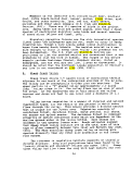 323% more successful nests than a nearby site with similar
vegetation (Comet and Wilson, 1994). Habitats on the valley-
walls adjacent to the valley floor have notably fewer songbirds
(Wilson and Comet, 1993). Many of the song bird species found in
Sheep Creek valley are of special interest. Five species whose
abundance is thought to be in decline in Alaska breed in the
valley. These are the fox sparrow, orange crowned warbler
blackpoll warbler, American robin, and varied thrush (Wilson and
Comet, 1991). Eight other species found in the valley may be
increasing in abundance. Fifteen of the 42 species of birds
documented during formal censusing are of interest to the
national program on neotropical birds (Wilson and Comet, 1991).
One additional bird, the marbled murrlet, whose use of the valley
has not been documented, is of concern because of population
declines along the west coast of North America.
Aquatic resources of the upper portion of Sheep Creek
include a local population of Dolly Vardon char. This population
is isolated from immigration from other char populations by
barriers to fish migration in the lower reach of Sheep Creek.
The lower 1.1 miles of the stream flows through a sequence
of cascades and falls to tidewater at Gastineau Channel 3.5 miles
south of downtown Juneau. A Douglas Island Pink and Chum
(DIPAC) hatchery is located at the mouth of Sheep Creek. The
hatchery produces pink and chum salmon for the recreation and
commercial fisheries of the area. Before merging with Gastineau
Channel, Sheep Creek crosses.an alluvial fan formed by sediments
carried by stream action from Sheep Creek valley above. Pink and
chum salmon spawn in the Sheep Creek upstream as far as an
impassible waterfall 440 feet above tidewater (BLM, 1992).
C. Gastineau Channel
Gastineau Channel is a north-south oriented channel
separating Douglas Island from the mainland. The shoreline for
approximately 10 miles between Stephens Passage and Juneau is
largely steep sided and rocky. Sediments from Mendenhall Glacier
have filled much of the channel to the north of downtown Juneau,
so that a tidal channel exists in this area.
According to studies of nearby Auk Bay, much of the
productivity of Gastineau Channel is likely tied to phytoplankton
blooms that occur as environmental factors, such as day length,
water temperature and nutrient levels, become more favorable in
the spring. These primary producers support zooplankton which in
turn support fisheries of commercial importance. The zooplankton
also includes larval fish which may also be of commercial and
ecological significance (BLM, 1992). At least 24 larval fish
species have been collected in Auk Bay (BLM, 1992). Gastineau
Channel is likely to contain similar numbers.
15
image:
323% more successful nests than a nearby site with similar
vegetation (Comet and Wilson, 1994). Habitats on the valley-
walls adjacent to the valley floor have notably fewer songbirds
(Wilson and Comet, 1993). Many of the song bird species found in
Sheep Creek valley are of special interest. Five species whose
abundance is thought to be in decline in Alaska breed in the
valley. These are the fox sparrow, orange crowned warbler
blackpoll warbler, American robin, and varied thrush (Wilson and
Comet, 1991). Eight other species found in the valley may be
increasing in abundance. Fifteen of the 42 species of birds
documented during formal censusing are of interest to the
national program on neotropical birds (Wilson and Comet, 1991).
One additional bird, the marbled murrlet, whose use of the valley
has not been documented, is of concern because of population
declines along the west coast of North America.
Aquatic resources of the upper portion of Sheep Creek
include a local population of Dolly Vardon char. This population
is isolated from immigration from other char populations by
barriers to fish migration in the lower reach of Sheep Creek.
The lower 1.1 miles of the stream flows through a sequence
of cascades and falls to tidewater at Gastineau Channel 3.5 miles
south of downtown Juneau. A Douglas Island Pink and Chum
(DIPAC) hatchery is located at the mouth of Sheep Creek. The
hatchery produces pink and chum salmon for the recreation and
commercial fisheries of the area. Before merging with Gastineau
Channel, Sheep Creek crosses.an alluvial fan formed by sediments
carried by stream action from Sheep Creek valley above. Pink and
chum salmon spawn in the Sheep Creek upstream as far as an
impassible waterfall 440 feet above tidewater (BLM, 1992).
C. Gastineau Channel
Gastineau Channel is a north-south oriented channel
separating Douglas Island from the mainland. The shoreline for
approximately 10 miles between Stephens Passage and Juneau is
largely steep sided and rocky. Sediments from Mendenhall Glacier
have filled much of the channel to the north of downtown Juneau,
so that a tidal channel exists in this area.
According to studies of nearby Auk Bay, much of the
productivity of Gastineau Channel is likely tied to phytoplankton
blooms that occur as environmental factors, such as day length,
water temperature and nutrient levels, become more favorable in
the spring. These primary producers support zooplankton which in
turn support fisheries of commercial importance. The zooplankton
also includes larval fish which may also be of commercial and
ecological significance (BLM, 1992). At least 24 larval fish
species have been collected in Auk Bay (BLM, 1992). Gastineau
Channel is likely to contain similar numbers.
15
image:
 Planktonic productivity typically exceeds grazing rates of
zooplankton, allowing much of the fixed carbon to settle to the
bottom, feeding the benthic community (BLM, 1992). Forty species
of demersal fish, shellfish and other invertebrates have been
reported from Gastineau Channel. Included among these are
commercially important crab species. The commercial crab fishery
was closed in 1978 but a popular personal use fishery continues
(BLM, 1992) .
Intertidal and subtidal flora and fauna of Gastineau Channel
is typical of protected shorelines of southeast Alaska. A
mussel-barnacle-rockweed (Mytilus-Balanus-Fucus) assemblage is
found on upper to mid-intertidal zones. Near the Sheep Creek
delta the substrate can be covered by up to 100% mussels. Green
sea urchin (Strongylocentrotus droJbachiensis), and several sea
star species were observed in this area during surveys associated
with this mine project (BLM, 1992) .
Much of the shore adjacent to the City of Juneau is composed
of tailings deposited during previous mining of the AJ Mine.
Surveys of these areas found reduced numbers of epifaunal and
infaunal organisms compared to locations that were not composed
of tailings (BLM, 1992).
16
image:
Planktonic productivity typically exceeds grazing rates of
zooplankton, allowing much of the fixed carbon to settle to the
bottom, feeding the benthic community (BLM, 1992). Forty species
of demersal fish, shellfish and other invertebrates have been
reported from Gastineau Channel. Included among these are
commercially important crab species. The commercial crab fishery
was closed in 1978 but a popular personal use fishery continues
(BLM, 1992) .
Intertidal and subtidal flora and fauna of Gastineau Channel
is typical of protected shorelines of southeast Alaska. A
mussel-barnacle-rockweed (Mytilus-Balanus-Fucus) assemblage is
found on upper to mid-intertidal zones. Near the Sheep Creek
delta the substrate can be covered by up to 100% mussels. Green
sea urchin (Strongylocentrotus droJbachiensis), and several sea
star species were observed in this area during surveys associated
with this mine project (BLM, 1992) .
Much of the shore adjacent to the City of Juneau is composed
of tailings deposited during previous mining of the AJ Mine.
Surveys of these areas found reduced numbers of epifaunal and
infaunal organisms compared to locations that were not composed
of tailings (BLM, 1992).
16
image:
 VI. EVALUATION OF PROJECTED TAILINGS POND PERFORMANCE
A. Introduction
Echo Bay has proposed the tailings impoundment as the sole
method of wastewater treatment for the AJ project. The
impoundment would be operated to allow for the settling of solids
that are delivered to the pond in the tailings slurry and surface
runoff. At the AJ project, the tailings slurry would be
comprised of approximately 55% solids by weight. This equates to
938,000 mg/1 of total suspended solids (TSS) when the slurry is
introduced to the tailings pond. EPA's New source Performance
Standards (NSPS) that apply to gold mining projects like AJ limit
TSS in the discharge from the impoundment to a monthly average of
20 mg/1 and a daily maximum of 30 mg/1. Therefore, the tailings
pond would need to be capable of removing over 99.99% of the
solids.
NSPS are minimum, technology-based effluent limits that
apply to a single industrial category of "new source" wastewater
dischargers. These limits must be met at the point of discharge
(end-of-pipe). More stringent effluent limits may be imposed on
a case-by-case basis if necessary to meet WQS. In theory, by
meeting the TSS limits, NSPS effluent limits for metals would be
met as well, since metals tend to be adsorbed on to the surface
of suspended particles. However, this may not be sufficient
metals removal for meeting water quality standards (WQS). Some
natural degradation of cyanide may occur during summer months but
for this analysis it is assumed that all cyanide destruction
would take place prior to discharge to the impoundment.
Predictions of the origin and fate of materials entering the
impoundment are critical for determining compliance with NPDES
requirements and the risk of long term contamination. As shown
in Figure 3, results of the impoundment analysis are subsequently
used in evaluations of end-of-pipe performance standards, water
quality impacts to Gastineau Channel, and the risk of long term
contamination in the reservoir following cessation of mining
activity.
The following major features of the impoundment system would
affect its performance in removing pollutants:
Quality and quantity of tailings influent (slurry) from
the froth flotation and cyanide leach circuits;
Quality and quantity of runoff from the undiverted
catchment area;
Settling efficiency of the tailings impoundment' under
low flow, average flow and high flow conditions;
17
image:
VI. EVALUATION OF PROJECTED TAILINGS POND PERFORMANCE
A. Introduction
Echo Bay has proposed the tailings impoundment as the sole
method of wastewater treatment for the AJ project. The
impoundment would be operated to allow for the settling of solids
that are delivered to the pond in the tailings slurry and surface
runoff. At the AJ project, the tailings slurry would be
comprised of approximately 55% solids by weight. This equates to
938,000 mg/1 of total suspended solids (TSS) when the slurry is
introduced to the tailings pond. EPA's New source Performance
Standards (NSPS) that apply to gold mining projects like AJ limit
TSS in the discharge from the impoundment to a monthly average of
20 mg/1 and a daily maximum of 30 mg/1. Therefore, the tailings
pond would need to be capable of removing over 99.99% of the
solids.
NSPS are minimum, technology-based effluent limits that
apply to a single industrial category of "new source" wastewater
dischargers. These limits must be met at the point of discharge
(end-of-pipe). More stringent effluent limits may be imposed on
a case-by-case basis if necessary to meet WQS. In theory, by
meeting the TSS limits, NSPS effluent limits for metals would be
met as well, since metals tend to be adsorbed on to the surface
of suspended particles. However, this may not be sufficient
metals removal for meeting water quality standards (WQS). Some
natural degradation of cyanide may occur during summer months but
for this analysis it is assumed that all cyanide destruction
would take place prior to discharge to the impoundment.
Predictions of the origin and fate of materials entering the
impoundment are critical for determining compliance with NPDES
requirements and the risk of long term contamination. As shown
in Figure 3, results of the impoundment analysis are subsequently
used in evaluations of end-of-pipe performance standards, water
quality impacts to Gastineau Channel, and the risk of long term
contamination in the reservoir following cessation of mining
activity.
The following major features of the impoundment system would
affect its performance in removing pollutants:
Quality and quantity of tailings influent (slurry) from
the froth flotation and cyanide leach circuits;
Quality and quantity of runoff from the undiverted
catchment area;
Settling efficiency of the tailings impoundment' under
low flow, average flow and high flow conditions;
17
image:
 Chapter VI
Impoundment Water Quality
Model
Chapter VII
Gastineau Channel Model
Chapter VI
Impoundment Water Quality
Model (Post Operation)
Chapter VI
Technology Evaluation
- New Source Performance
Standards
Chapter VII
Water Quality Evaluation
- Gastineau Channel
Chapter VIII
Ecological Risk Evaluation
- Sheep Creek Reservoir
Rgure 3: Modeling and Assessment Linkages
image:
Chapter VI
Impoundment Water Quality
Model
Chapter VII
Gastineau Channel Model
Chapter VI
Impoundment Water Quality
Model (Post Operation)
Chapter VI
Technology Evaluation
- New Source Performance
Standards
Chapter VII
Water Quality Evaluation
- Gastineau Channel
Chapter VIII
Ecological Risk Evaluation
- Sheep Creek Reservoir
Rgure 3: Modeling and Assessment Linkages
image:
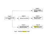 Size .of the tailings pond and diversion structures in •
relation to anticipated high flows;
Vulnerability of the impoundment to natural hazards
such as avalanches, landslides and earthquakes.
There are two basic approaches for projections of
impoundment performance. The first is to consider all of the
inputs (influent) and outputs (effluent) to and from the tailings
pond, respectively, and then, using water quality modeling,
analyze the pond's effectiveness in terms of removing pollutants
and thus estimate the projected composition of the effluent.
This approach, using a simplistic model, was used during the EIS
process to project the quality of the effluent. Our review
entailed more sophisticated water quality modeling using the
WASP4 and CE-Qual-W2 water quality models.
The second approach is to compare the AJ project to other
mining operations that employ the same or similar technology.
The reliability of this empirical approach hinges on the direct
comparability between the AJ project and the other mines that are
examined.
The next two sections of this chapter present brief
overviews of the NPDES requirements for this project and the FEIS
evaluation of the impoundment. The subsequent sections present
EPA's analysis and projections of impoundment performance.
B^_ NPDES Requirements
An NPDES permit is required for the point source discharge
from the tailings impoundment. Two sets of requirements^must be
met by the discharge from the proposed AJ impoundment. First,
the discharge must meet the national New Source Performance
Standards at the point of discharge from the impoundment (end-of-
pipe) These limitations on metals, cyanide and suspended solids
apply to all mining facilities using the froth flotation and
cvanidation processes proposed for use at the AJ project (40 CFR
III 104(a° Subpart J). A comparison of the predicted discharge^
quality with these end-of-pipe limitations is provided in section
I of this chapter.
The second set of NPDES requirements are the Alaska water
quality standards for Gastineau Channel. Discharges from the AJ
project must meet numeric water quality criteria for the
nrotection of beneficial uses in Gastineau Channel.
?neci?icallv the criteria are established to protect against
SxiciS io^qualic life from exposure to pollutants in the water
column and effects to human health from consumption of
contaminated fish and shellfish. These criteria must be met
SithS £ the end-of-pipe or after dilution in a mixing zone
designated by ?he sta?eof Alaska. An evaluation of the
19
image:
Size .of the tailings pond and diversion structures in •
relation to anticipated high flows;
Vulnerability of the impoundment to natural hazards
such as avalanches, landslides and earthquakes.
There are two basic approaches for projections of
impoundment performance. The first is to consider all of the
inputs (influent) and outputs (effluent) to and from the tailings
pond, respectively, and then, using water quality modeling,
analyze the pond's effectiveness in terms of removing pollutants
and thus estimate the projected composition of the effluent.
This approach, using a simplistic model, was used during the EIS
process to project the quality of the effluent. Our review
entailed more sophisticated water quality modeling using the
WASP4 and CE-Qual-W2 water quality models.
The second approach is to compare the AJ project to other
mining operations that employ the same or similar technology.
The reliability of this empirical approach hinges on the direct
comparability between the AJ project and the other mines that are
examined.
The next two sections of this chapter present brief
overviews of the NPDES requirements for this project and the FEIS
evaluation of the impoundment. The subsequent sections present
EPA's analysis and projections of impoundment performance.
B^_ NPDES Requirements
An NPDES permit is required for the point source discharge
from the tailings impoundment. Two sets of requirements^must be
met by the discharge from the proposed AJ impoundment. First,
the discharge must meet the national New Source Performance
Standards at the point of discharge from the impoundment (end-of-
pipe) These limitations on metals, cyanide and suspended solids
apply to all mining facilities using the froth flotation and
cvanidation processes proposed for use at the AJ project (40 CFR
III 104(a° Subpart J). A comparison of the predicted discharge^
quality with these end-of-pipe limitations is provided in section
I of this chapter.
The second set of NPDES requirements are the Alaska water
quality standards for Gastineau Channel. Discharges from the AJ
project must meet numeric water quality criteria for the
nrotection of beneficial uses in Gastineau Channel.
?neci?icallv the criteria are established to protect against
SxiciS io^qualic life from exposure to pollutants in the water
column and effects to human health from consumption of
contaminated fish and shellfish. These criteria must be met
SithS £ the end-of-pipe or after dilution in a mixing zone
designated by ?he sta?eof Alaska. An evaluation of the
19
image:
 predicted discharge quality with respect to the water quality
standards for Gastineau Channel is provided in Chapter VII of
this report.
C_-_ Review of the FEIS Water Quality Model
Water quality analyses of the proposed tailings pond, as
described in the FEIS and errata to the FEIS (Tileston, 1992) ,
provided a limited examination of the metals concentrations in
the tailings pond using estimates from the literature and results
of laboratory tests. Based on these initial estimates, the FEIS
for this project predicted that "Suspended solids (TSS) content
is likely to be at least 70 mg/1 near the discharge, and may be
as much as 220 mg/1 throughout the entire impoundment." These
-values exceed the levels required by EPA's NSPS for mine tailings
ponds. However, the methodology used in the FEIS to estimate
levels of TSS and important chemical constituents in the proposed
tailings pond was based on static, rather than dynamic
conditions. In addition, the methods used in the FEIS to
-estimate the recovery time of the tailings pond after mining
ceases gave results substantially different from recovery times
based on average residence time of the tailings pond.
Due to the limited scope of the analysis performed in the
FEIS, and results indicating that NSPS effluent limits for TSS
would not be met, EPA Region 10 concluded that a more thorough
analysis of water quality should be performed for purposes of the
TAR. The approach used in the analysis described in this report
represents an effort to clarify issues of mass balance as well as
to expand the scope of the analysis to include issues of time
dependence; sediment accumulation rates; inputs of kinetic energy
from discharges, and winds. Characterizing the influent to the
pond, discussed in the following section, is a critical first
step in the analysis.
D^ characteristics of Process Influent to the Tailings Pond.
Water quality predictions for the tailings pond and
discharge are based in part on estimates of the chemical
composition of process materials that flow into the pond from the
mill. A reevaluation of the approach, sources of data, and
results of influent estimates provided in the FEIS and subsequent
FEIS errata tables (Tileston, 1992) is provided here, along with
improved estimates used for subsequent water quality modeling.
1. FEIS Approach
Estimates in the FEIS for the chemical composition of
tailings pond influent from Echo Bay minerals processing were
based on a variety of methods involving site specific field and
lab data as well as assumed operating conditions. The FEIS
Approach" uLs what are termed "probable threshold" and "upper
20
image:
predicted discharge quality with respect to the water quality
standards for Gastineau Channel is provided in Chapter VII of
this report.
C_-_ Review of the FEIS Water Quality Model
Water quality analyses of the proposed tailings pond, as
described in the FEIS and errata to the FEIS (Tileston, 1992) ,
provided a limited examination of the metals concentrations in
the tailings pond using estimates from the literature and results
of laboratory tests. Based on these initial estimates, the FEIS
for this project predicted that "Suspended solids (TSS) content
is likely to be at least 70 mg/1 near the discharge, and may be
as much as 220 mg/1 throughout the entire impoundment." These
-values exceed the levels required by EPA's NSPS for mine tailings
ponds. However, the methodology used in the FEIS to estimate
levels of TSS and important chemical constituents in the proposed
tailings pond was based on static, rather than dynamic
conditions. In addition, the methods used in the FEIS to
-estimate the recovery time of the tailings pond after mining
ceases gave results substantially different from recovery times
based on average residence time of the tailings pond.
Due to the limited scope of the analysis performed in the
FEIS, and results indicating that NSPS effluent limits for TSS
would not be met, EPA Region 10 concluded that a more thorough
analysis of water quality should be performed for purposes of the
TAR. The approach used in the analysis described in this report
represents an effort to clarify issues of mass balance as well as
to expand the scope of the analysis to include issues of time
dependence; sediment accumulation rates; inputs of kinetic energy
from discharges, and winds. Characterizing the influent to the
pond, discussed in the following section, is a critical first
step in the analysis.
D^ characteristics of Process Influent to the Tailings Pond.
Water quality predictions for the tailings pond and
discharge are based in part on estimates of the chemical
composition of process materials that flow into the pond from the
mill. A reevaluation of the approach, sources of data, and
results of influent estimates provided in the FEIS and subsequent
FEIS errata tables (Tileston, 1992) is provided here, along with
improved estimates used for subsequent water quality modeling.
1. FEIS Approach
Estimates in the FEIS for the chemical composition of
tailings pond influent from Echo Bay minerals processing were
based on a variety of methods involving site specific field and
lab data as well as assumed operating conditions. The FEIS
Approach" uLs what are termed "probable threshold" and "upper
20
image:
 reasonable threshold" values for projected quality of process
effluent (BLM, 1992, Table 4-8) which becomes the influent to the
tailings pond.
Probable threshold is defined in the FEIS (Table 4-8; BLM,
1992) as the average water concentration resulting from
dissimilar lab tests, including the following:
1. The sum of flow-weighted values from separate decant tests
of flotation and cyanide-destruct (CIL) tailings. The FEIS
notes that the- values used from the decant tests are the
maximum measured from four samples of water collected during
a 99-day settling period. The flow weighting used in the
FEIS assumes a proportion of about 23% of CIL process water,
based on the water balance shown in the FEIS (Table 4-8 and
Figure 2-17; BLM, 1992).
2. Maximum values from a decant test of combined flotation and
CIL tailings. The mix used in the combined tailings
contained 10% wet-weight (w/w) CIL tails. This test also
provided samples at four settling times spanning 99 days.
3. Maximum values of weekly samples drawn during column leach
tests conducted on combined flotation and CIL tailings. The
leachant was Sheep Creek water. The proportion of CIL
tailings was 10% w/w. The column tests spanned 105-140
days.
4. The FEIS limited the probable threshold values for some
constituents based on the results of either a total
digestion or slurry extract of combined tailings.
Upper reasonable threshold is defined in the FEIS (Table 4-
8) as the maximum rather than the average of. all of the values
noted above, but not exceeding the results from the total
digestion or slurry extract of tailings. Table 3 lists a summary
of the types of lab tests that provide data useful for estimating
contaminant concentrations in the tailings influent to the pond,
as well as the risk of long-term contamination addressed in
Section VIII-N. Table 4 lists information on the source and
timing of lab tests, and Tables B-l and B-2 in Appendix B provide
a compilation of decant, column, digest and slurry results for
tailings.
2_._ Validity of the FEIS Approach
Examination of available lab data for purposes of this
report indicates that the FEIS approach probably yields neither
most probable nor upper bound values for some of the more
important constituents in the tailings pond influent. An initial
concern was that FEIS values presented for digested tailings
21
image:
reasonable threshold" values for projected quality of process
effluent (BLM, 1992, Table 4-8) which becomes the influent to the
tailings pond.
Probable threshold is defined in the FEIS (Table 4-8; BLM,
1992) as the average water concentration resulting from
dissimilar lab tests, including the following:
1. The sum of flow-weighted values from separate decant tests
of flotation and cyanide-destruct (CIL) tailings. The FEIS
notes that the- values used from the decant tests are the
maximum measured from four samples of water collected during
a 99-day settling period. The flow weighting used in the
FEIS assumes a proportion of about 23% of CIL process water,
based on the water balance shown in the FEIS (Table 4-8 and
Figure 2-17; BLM, 1992).
2. Maximum values from a decant test of combined flotation and
CIL tailings. The mix used in the combined tailings
contained 10% wet-weight (w/w) CIL tails. This test also
provided samples at four settling times spanning 99 days.
3. Maximum values of weekly samples drawn during column leach
tests conducted on combined flotation and CIL tailings. The
leachant was Sheep Creek water. The proportion of CIL
tailings was 10% w/w. The column tests spanned 105-140
days.
4. The FEIS limited the probable threshold values for some
constituents based on the results of either a total
digestion or slurry extract of combined tailings.
Upper reasonable threshold is defined in the FEIS (Table 4-
8) as the maximum rather than the average of. all of the values
noted above, but not exceeding the results from the total
digestion or slurry extract of tailings. Table 3 lists a summary
of the types of lab tests that provide data useful for estimating
contaminant concentrations in the tailings influent to the pond,
as well as the risk of long-term contamination addressed in
Section VIII-N. Table 4 lists information on the source and
timing of lab tests, and Tables B-l and B-2 in Appendix B provide
a compilation of decant, column, digest and slurry results for
tailings.
2_._ Validity of the FEIS Approach
Examination of available lab data for purposes of this
report indicates that the FEIS approach probably yields neither
most probable nor upper bound values for some of the more
important constituents in the tailings pond influent. An initial
concern was that FEIS values presented for digested tailings
21
image:
 Table 3. Type* of Test Data Available for the A-J Project to nrfnm« die Composition of Tailing*, Tailings Pore Water, Tailings Leacbate,
and Acid Generation Potential -
Concentrations in Tailings Water
Decani Test
Concentration of metals, cyanide, and other nonmetals in supernatant measured at 2-hour, 7-day, 30-day, and 99-day intervals.
Material tested
Flotation Tailings
CO. Tailings
Physically Combined Tailings (10% w/w CO. tailings)
Concentrations in Tailings Solids
Digestion Analysis
Concentration of metals in solid fraction of tailing*
Material tested
Physically Combined Tailing* (10% w/w COL tailings)
Slurry Extraction Analysis
Concentration of cyanide and non-metals in extract of stony of tailing* and water (Note-conditions of thi* test are unknown)
Material tested
Physically Combined Tailing* (10% w/w CIL tailings)
Ore analyses (indirect tmimf'f of tailing* Maiming similarity)
Concentration of metals and sulfur in solid fraction of tailings
Material tested
Bulk sample of ore
Core samples of ore
Grab samples of ore
Concentrations in Tailings Leaehate
Column Leach Tests
Concentration of metals, cyanide, and other non-metals at periodic intervals over 12-20 weeks.
Material tested
Physically Combined Tailings (10% CO. toiling*)
Batch Leach Testa .
EFTox (Extraction Procedure Toxkiry) - Concentration of metals in 48-hour tumbling container. Previously used for comparison
wiih criteria for himmlou* wute drpgnalion
TCLPfToxkity Criteria U«^ Procedure)-Oaweitotion of mettUm 4^^ Used for comparison
with criteria for hazardous waste designation
Material tested
Physically Combined Tailings (10% CO. tailings)
Acid Generation Potential Testj
Acid-Ba*e Accounting (ABA) Test
Concentration of oxidizing component* (sulfiir) and ijeuttmBziiig cwi^wnentt (Utrattble reactaats)
Material tested
Waste rock
On
Flotation Tailings
CO. Tailings
Physically Combined Tailings (10% w/w CIL tailings)
BC Confirmation Column test
pH trend in acidified, bacteria-inoculated sample
Material tested
Flotation Tailings
CIL Tailings
image:
Table 3. Type* of Test Data Available for the A-J Project to nrfnm« die Composition of Tailing*, Tailings Pore Water, Tailings Leacbate,
and Acid Generation Potential -
Concentrations in Tailings Water
Decani Test
Concentration of metals, cyanide, and other nonmetals in supernatant measured at 2-hour, 7-day, 30-day, and 99-day intervals.
Material tested
Flotation Tailings
CO. Tailings
Physically Combined Tailings (10% w/w CO. tailings)
Concentrations in Tailings Solids
Digestion Analysis
Concentration of metals in solid fraction of tailing*
Material tested
Physically Combined Tailing* (10% w/w COL tailings)
Slurry Extraction Analysis
Concentration of cyanide and non-metals in extract of stony of tailing* and water (Note-conditions of thi* test are unknown)
Material tested
Physically Combined Tailing* (10% w/w CIL tailings)
Ore analyses (indirect tmimf'f of tailing* Maiming similarity)
Concentration of metals and sulfur in solid fraction of tailings
Material tested
Bulk sample of ore
Core samples of ore
Grab samples of ore
Concentrations in Tailings Leaehate
Column Leach Tests
Concentration of metals, cyanide, and other non-metals at periodic intervals over 12-20 weeks.
Material tested
Physically Combined Tailings (10% CO. toiling*)
Batch Leach Testa .
EFTox (Extraction Procedure Toxkiry) - Concentration of metals in 48-hour tumbling container. Previously used for comparison
wiih criteria for himmlou* wute drpgnalion
TCLPfToxkity Criteria U«^ Procedure)-Oaweitotion of mettUm 4^^ Used for comparison
with criteria for hazardous waste designation
Material tested
Physically Combined Tailings (10% CO. tailings)
Acid Generation Potential Testj
Acid-Ba*e Accounting (ABA) Test
Concentration of oxidizing component* (sulfiir) and ijeuttmBziiig cwi^wnentt (Utrattble reactaats)
Material tested
Waste rock
On
Flotation Tailings
CO. Tailings
Physically Combined Tailings (10% w/w CIL tailings)
BC Confirmation Column test
pH trend in acidified, bacteria-inoculated sample
Material tested
Flotation Tailings
CIL Tailings
image:
 AJCOMPI XIS
M«»rlrf
Hock IBionipla*
WMI* lock nockpU* • 6 stvnplet
Oit • bulk tiwnjjla
Ttvllna* - comtko <b*cnd)
On • bulk »ampl« (1441)
lallngi - Flot/CND/comtK>(12*>
T*tllnfl» dccwit i«Bldut? CN/CND
Taillno* d«c«nt inldtM
Tailing.* dacant ia»tdtM
Oi» • 6 channel »mplM
Wa*u tocfc • 34 sOTiplM
W*»i« tocfc • 63 Mmplm
Oi« • 36 >MnplM
Ol« • 101 CIO*KUl MTTIfrfM
Ol* • 102 CO(« Mmple*
Oi* • 63 ctottcut ••inplM
Souic*
NOB-SOB GH other
unknown
NOB-SOB
unknown
NOB |* AT, 43B7SX)
NOBI'AJ*. 4387SX)
NOB TAJ*. 43B7SX)
NOB ('AT, 43B7SX)
NOB CAJ-, 4387SX)
MOBrAJ-,43B7S«
NOB I43B7SX)
NOB-lo«d
NOB-SOB
NOB SOB
NOB SOB
NOBSOB
NOB SOB
NOB • nonh oi« body; SOB • »outh 01* body.
Sampled
/87
unknown
6/686/69
e/es
e/68
e/ee
8/88
9/88
»/ee
treat
3/04
6/«4r
3/84
6/M
1
r
MIDad
7/88J
6/89?
7/80
Meiii
/asr
E/88
/Q8f
71807
Dl?
flSl
6/14
Sulluf
mlslJnB
6/88
/887
6/8B)
/887
7/60r
Set
4/84
6/64 .
3/»4
6/84
6/84
ABA
6/ie
11/80
4/84
6/84
3/84
6/84
6/84
OKMt
7AKMO/90
Conllrm
11/80
CN
<r*£*sa —
FKtIKt
3IJ
Cofunm
e/a»
3/81-7/81
IITOX
TCLP
R«l*i6nc«
Etoto.ll torn |
Oil (1089).
on (1888)
L*elMd He
Oil H889)
1884.)
M«c<i(18e
Bttantom t
IOB4b). EBA
8.1
18846). (B/
.(1884.)
(1084.)
Lekelleld RiMudi (1B80) «id Andr«w> (18811
IdulleMRMMidiliea
Baigvtfom (1804b)
9<ig«ionil1884li)
Andiowi (1 881); Jokite
)), Andiawa
(19811. mi
bidimn 118811 «nd FEIS (1883)
Fitdeitc*«oo
BA|I»04.
"~1
(1882). (I
:BA(1884>)
I
:BA(1884«)
BA(I8B4«)
3A(iee*«)
8A|1884b)
1(18844)
SSI 1
1881), •«!
ftIS (1882
toiflrtTOm \
^-^™^^-^™«
B84bl
—
~
image:
AJCOMPI XIS
M«»rlrf
Hock IBionipla*
WMI* lock nockpU* • 6 stvnplet
Oit • bulk tiwnjjla
Ttvllna* - comtko <b*cnd)
On • bulk »ampl« (1441)
lallngi - Flot/CND/comtK>(12*>
T*tllnfl» dccwit i«Bldut? CN/CND
Taillno* d«c«nt inldtM
Tailing.* dacant ia»tdtM
Oi» • 6 channel »mplM
Wa*u tocfc • 34 sOTiplM
W*»i« tocfc • 63 Mmplm
Oi« • 36 >MnplM
Ol« • 101 CIO*KUl MTTIfrfM
Ol* • 102 CO(« Mmple*
Oi* • 63 ctottcut ••inplM
Souic*
NOB-SOB GH other
unknown
NOB-SOB
unknown
NOB |* AT, 43B7SX)
NOBI'AJ*. 4387SX)
NOB TAJ*. 43B7SX)
NOB ('AT, 43B7SX)
NOB CAJ-, 4387SX)
MOBrAJ-,43B7S«
NOB I43B7SX)
NOB-lo«d
NOB-SOB
NOB SOB
NOB SOB
NOBSOB
NOB SOB
NOB • nonh oi« body; SOB • »outh 01* body.
Sampled
/87
unknown
6/686/69
e/es
e/68
e/ee
8/88
9/88
»/ee
treat
3/04
6/«4r
3/84
6/M
1
r
MIDad
7/88J
6/89?
7/80
Meiii
/asr
E/88
/Q8f
71807
Dl?
flSl
6/14
Sulluf
mlslJnB
6/88
/887
6/8B)
/887
7/60r
Set
4/84
6/64 .
3/»4
6/84
6/84
ABA
6/ie
11/80
4/84
6/84
3/84
6/84
6/84
OKMt
7AKMO/90
Conllrm
11/80
CN
<r*£*sa —
FKtIKt
3IJ
Cofunm
e/a»
3/81-7/81
IITOX
TCLP
R«l*i6nc«
Etoto.ll torn |
Oil (1089).
on (1888)
L*elMd He
Oil H889)
1884.)
M«c<i(18e
Bttantom t
IOB4b). EBA
8.1
18846). (B/
.(1884.)
(1084.)
Lekelleld RiMudi (1B80) «id Andr«w> (18811
IdulleMRMMidiliea
Baigvtfom (1804b)
9<ig«ionil1884li)
Andiowi (1 881); Jokite
)), Andiawa
(19811. mi
bidimn 118811 «nd FEIS (1883)
Fitdeitc*«oo
BA|I»04.
"~1
(1882). (I
:BA(1884>)
I
:BA(1884«)
BA(I8B4«)
3A(iee*«)
8A|1884b)
1(18844)
SSI 1
1881), •«!
ftIS (1882
toiflrtTOm \
^-^™^^-^™«
B84bl
—
~
image:
 seemed unrealistically low. The impact was that these values
were subsequently used as an upper bound for some of the FEIS-
predicted constituents in the process effluent. After completion
of the FEIS, an updated Table 8 which adjusted the digested
tailings values upward was provided by the FEIS contractor
(Tileston, 1992). The updated values are listed here in Table 5
under the heading FEIS.
Comparison of the updated FEIS Table 4.-8 values with
laboratory reports upon which they were based indicates that for
several constituents the maximum decant values measured in the
lab tests were not used for effluent quality projections in all
cases. The discrepancy appears to result, at least in part, from
use of total analytical values in the FEIS table, even though the
lab reports show that in some cases total recoverable or
dissolved values are greater. The impact of using all available
decant data in a manner consistent with the approach described in
the FEIS would be to increase somewhat the projected tailings
concentrations for some constituents. Table 5 lists these
revisions under .the heading FEIS REV.
Other potential problems with the FEIS approach to effluent
quality projections include incomplete information on the
representativeness and variability of materials being tested, and
the averaging of data from dissimilar tests without regard to the
chemical reactions being tested.
With respect to representativeness of materials, Table 4
provides a list of the source and times of various tests
conducted for the AJ project. Tailings tests used for the FEIS
effluent projections are based on a single bulk sample collected
from the 4387SX crosscut in the north ore body in 1988 (EBA,
1994a). In a recent report, the applicant contends that the
single bulk ore sample is representative of average.
concentrations of material to be mined. A single tailings sample
therefore may provide useful data for evaluating average
conditions but no information on variability to be expected if
the mill feed varies during production. Consequently,
projections based on any of the various tests of the bulk sample
products cannot necessarily be representative of worst or "upper
reasonable threshold" conditions, because the sample is not
necessarily worst case. Accordingly, the "upper reasonable
threshold" conditions as listed in the FEIS should not be
considered worst-case effluent quality.
The proportion of CIL tailings varies among the tests used
in the FEIS projections. The only estimates based on a 23% mix
of CIL tailings water as used in the FEIS water balance are the
mathematically derived flow-weighted combinations of decant data
from separately settled flotation and CIL tailings. Since much
of the higher contaminant load is from the CIL tailings,
24
image:
seemed unrealistically low. The impact was that these values
were subsequently used as an upper bound for some of the FEIS-
predicted constituents in the process effluent. After completion
of the FEIS, an updated Table 8 which adjusted the digested
tailings values upward was provided by the FEIS contractor
(Tileston, 1992). The updated values are listed here in Table 5
under the heading FEIS.
Comparison of the updated FEIS Table 4.-8 values with
laboratory reports upon which they were based indicates that for
several constituents the maximum decant values measured in the
lab tests were not used for effluent quality projections in all
cases. The discrepancy appears to result, at least in part, from
use of total analytical values in the FEIS table, even though the
lab reports show that in some cases total recoverable or
dissolved values are greater. The impact of using all available
decant data in a manner consistent with the approach described in
the FEIS would be to increase somewhat the projected tailings
concentrations for some constituents. Table 5 lists these
revisions under .the heading FEIS REV.
Other potential problems with the FEIS approach to effluent
quality projections include incomplete information on the
representativeness and variability of materials being tested, and
the averaging of data from dissimilar tests without regard to the
chemical reactions being tested.
With respect to representativeness of materials, Table 4
provides a list of the source and times of various tests
conducted for the AJ project. Tailings tests used for the FEIS
effluent projections are based on a single bulk sample collected
from the 4387SX crosscut in the north ore body in 1988 (EBA,
1994a). In a recent report, the applicant contends that the
single bulk ore sample is representative of average.
concentrations of material to be mined. A single tailings sample
therefore may provide useful data for evaluating average
conditions but no information on variability to be expected if
the mill feed varies during production. Consequently,
projections based on any of the various tests of the bulk sample
products cannot necessarily be representative of worst or "upper
reasonable threshold" conditions, because the sample is not
necessarily worst case. Accordingly, the "upper reasonable
threshold" conditions as listed in the FEIS should not be
considered worst-case effluent quality.
The proportion of CIL tailings varies among the tests used
in the FEIS projections. The only estimates based on a 23% mix
of CIL tailings water as used in the FEIS water balance are the
mathematically derived flow-weighted combinations of decant data
from separately settled flotation and CIL tailings. Since much
of the higher contaminant load is from the CIL tailings,
24
image:
 AJPROAQ.XLS
Table 6. Projections of tailings composition - aqueous and solid fractions.
:low
pH
TDS
TSS
Turbidity
-lardness
Alkalinity
Sullate
Ammonia
Nitrate, N
Nitrite. N
TKN
FEIS
FEIS REV
FtDW-wl combination
3760
8.2
3200
14200
107
672
209
4000
17.6
20.4
0.69
80.1
Areenic 0,002 0.006
Cadmium
Chromium
Copper
Iron
Lead
Manganese
Mercury
Nickel
Selenium
Silver
Zinc
Xanthate
Free Cyanide
Total Cyanide
WAD Cyanide
Cyanale
Thiocyanate
Footnotes:
0.008
0.001
1.36
0.137
0,08
0.006
0.011
0.013
0.002
0.056
0.927
0.774
1.29
0.82
73.3
393
0.01
0.004
0.188
0.633
0.006
0.017
0.002
0.781
1.76
.
FEIS
FEIS REV
Pratubla ThnuhoM
7.6
1600
440
74
480
160
370
7.3
0,0042:
0,006*
'*, 0,00.7
o.ea
3
0.093
0.8
0.0011
0.014
„ 0,0055
"'•' 94V
0.17
0,6
1.1
0.19
28
, , ; W
1617
8.4
8.19
41.9
00047
- 00091
0.00.?$
0.81
0021
0.21
1.2
FEIS
FEIS REV
Uppar Raaaonabla Thravhold
8.2
3200
1400
260
670
210
4000
7.3
0.012
1.4
14
0.16
2.7
0.0054
0.022
0.013
0.47
0.6
1.1
2.5
0.82
73
390
18
20
0.69
80
0.024
0.005
0.03
0.017
0.69
0.93
•
FEIS
Diga<l
mo/Va
9.78
11
35.4
262
45600
197
1660
0.274
26.7
FEIS
Slurry Extract
mgJVg
370
17
1,22
3,0ft
628
OA
42.4
p.e
FEIS - values from FEIS method, as listed in Corrected Tebla 4-8. letter from JMM to Oavid Dorrie, BLM, September 18, 1 992 (Tileston, 1992).
FEIS REV - Values from FEIS method derived from data tables in FEIS supporting documents.
TAR - values recommended for use in the Technical Analysis Report.
fwdec - flaw-weighted decant; codec - combined decant: 1 • leach; cnf - free cyanide
:5Wti(lnM:SS:: = less-then value
TAR
aquaout
b*.n
fwdec
fwdac
fwdac
codec
fwdec
fwdec
fwdec
fwdec
1
Iwdac
|
fwdec
1
TAR
•quaoua
ITQ/l
3200
670
210
1700
18
20
0.69
80
Q.OU
0.01
0,0?
1.3
0.85
TAR
talk)
ma /kg
370
17
9.8
11
35
260
46000
0,02 200
.wdec
wdec
codec
wdec
codec
cnf
wdec
wdec
2.7
0.005
0.03
0.016
0.0$
6.087
0.93
1.1
2.5
1.1
73
390
1600
0.27
26
" ' 1
3
630
Page 1
image:
AJPROAQ.XLS
Table 6. Projections of tailings composition - aqueous and solid fractions.
:low
pH
TDS
TSS
Turbidity
-lardness
Alkalinity
Sullate
Ammonia
Nitrate, N
Nitrite. N
TKN
FEIS
FEIS REV
FtDW-wl combination
3760
8.2
3200
14200
107
672
209
4000
17.6
20.4
0.69
80.1
Areenic 0,002 0.006
Cadmium
Chromium
Copper
Iron
Lead
Manganese
Mercury
Nickel
Selenium
Silver
Zinc
Xanthate
Free Cyanide
Total Cyanide
WAD Cyanide
Cyanale
Thiocyanate
Footnotes:
0.008
0.001
1.36
0.137
0,08
0.006
0.011
0.013
0.002
0.056
0.927
0.774
1.29
0.82
73.3
393
0.01
0.004
0.188
0.633
0.006
0.017
0.002
0.781
1.76
.
FEIS
FEIS REV
Pratubla ThnuhoM
7.6
1600
440
74
480
160
370
7.3
0,0042:
0,006*
'*, 0,00.7
o.ea
3
0.093
0.8
0.0011
0.014
„ 0,0055
"'•' 94V
0.17
0,6
1.1
0.19
28
, , ; W
1617
8.4
8.19
41.9
00047
- 00091
0.00.?$
0.81
0021
0.21
1.2
FEIS
FEIS REV
Uppar Raaaonabla Thravhold
8.2
3200
1400
260
670
210
4000
7.3
0.012
1.4
14
0.16
2.7
0.0054
0.022
0.013
0.47
0.6
1.1
2.5
0.82
73
390
18
20
0.69
80
0.024
0.005
0.03
0.017
0.69
0.93
•
FEIS
Diga<l
mo/Va
9.78
11
35.4
262
45600
197
1660
0.274
26.7
FEIS
Slurry Extract
mgJVg
370
17
1,22
3,0ft
628
OA
42.4
p.e
FEIS - values from FEIS method, as listed in Corrected Tebla 4-8. letter from JMM to Oavid Dorrie, BLM, September 18, 1 992 (Tileston, 1992).
FEIS REV - Values from FEIS method derived from data tables in FEIS supporting documents.
TAR - values recommended for use in the Technical Analysis Report.
fwdec - flaw-weighted decant; codec - combined decant: 1 • leach; cnf - free cyanide
:5Wti(lnM:SS:: = less-then value
TAR
aquaout
b*.n
fwdec
fwdac
fwdac
codec
fwdec
fwdec
fwdec
fwdec
1
Iwdac
|
fwdec
1
TAR
•quaoua
ITQ/l
3200
670
210
1700
18
20
0.69
80
Q.OU
0.01
0,0?
1.3
0.85
TAR
talk)
ma /kg
370
17
9.8
11
35
260
46000
0,02 200
.wdec
wdec
codec
wdec
codec
cnf
wdec
wdec
2.7
0.005
0.03
0.016
0.0$
6.087
0.93
1.1
2.5
1.1
73
390
1600
0.27
26
" ' 1
3
630
Page 1
image:
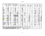 increasing the.-CIL proportion in any of the tests of combined
tailings would probably increase the concentrations of
contaminants in the tailings.
3. Alternative Approach
The FEIS approach considered dissolved and suspended
concentrations together as a total process effluent
concentration. An alternative approach used here is to consider
the tailings pond influent from the mill as an aqueous phase and
a solid phase, each with its own separate constituent
concentrations. Table 5 lists these values under the heading
TAR. Appendix B contains laboratory data listed in Tables B-l
and B-2 from which values in Table 5 are derived. Since these
data are from the same limited tests as used for the FEIS, the
limitations, as noted above, on being able to evaluate tailings
variablity or worse-than-average tailings concentrations apply.
Effluent "quality based on tailings produced from milling an
average bulk ore sample would not accurately project the total
range of contaminant concentration to be expected. To offset to
some degree the inherent underestimation of contaminant
concentrations that arises when using average samples, the use of
lab data described below emphasizies the higher values.
EPA's application of alternative influent values for this
analysis relies on the greater of either decant or column leach
data for the aqueous phase. Where decant data are used, the TAR •
values are from dissolved rather than total data. Mathematically
flow-weighted decant values are used where greater because they
represent the actual CIL proportions projected by the FEIS water
balance. Comparison of flow-weighted values at a 23% mix of CIL
water with the physically combined values of a mix of 10% CIL
tailings indicates that the two sets of data would have similar
initial decant results for many of the major parameters if the
CIL proportions were the same.
Digest and slurry extract data from the FEIS are used for
the solid phases in tailings. As with aqueous phase data, single
digest and extract analyses of tailings as reported in the FEIS
would not represent extreme values because of the reported (EBA,
1994b) average nature of the bulk sample.
JL_ Predictions of Effluent Quality; WASP4 Water Quality Model
1. Introduction
As described in the FEIS (BLM, 1992), the preferred
alternative entails converting most of the Sheep Creek valley
into a tailings disposal impoundment. While the proposed
facility is in operation, this impoundment would function as a
wastewater treatment facility for the tailings slurry discharge.
The water from the impoundment would be combined with excess flow
26
image:
increasing the.-CIL proportion in any of the tests of combined
tailings would probably increase the concentrations of
contaminants in the tailings.
3. Alternative Approach
The FEIS approach considered dissolved and suspended
concentrations together as a total process effluent
concentration. An alternative approach used here is to consider
the tailings pond influent from the mill as an aqueous phase and
a solid phase, each with its own separate constituent
concentrations. Table 5 lists these values under the heading
TAR. Appendix B contains laboratory data listed in Tables B-l
and B-2 from which values in Table 5 are derived. Since these
data are from the same limited tests as used for the FEIS, the
limitations, as noted above, on being able to evaluate tailings
variablity or worse-than-average tailings concentrations apply.
Effluent "quality based on tailings produced from milling an
average bulk ore sample would not accurately project the total
range of contaminant concentration to be expected. To offset to
some degree the inherent underestimation of contaminant
concentrations that arises when using average samples, the use of
lab data described below emphasizies the higher values.
EPA's application of alternative influent values for this
analysis relies on the greater of either decant or column leach
data for the aqueous phase. Where decant data are used, the TAR •
values are from dissolved rather than total data. Mathematically
flow-weighted decant values are used where greater because they
represent the actual CIL proportions projected by the FEIS water
balance. Comparison of flow-weighted values at a 23% mix of CIL
water with the physically combined values of a mix of 10% CIL
tailings indicates that the two sets of data would have similar
initial decant results for many of the major parameters if the
CIL proportions were the same.
Digest and slurry extract data from the FEIS are used for
the solid phases in tailings. As with aqueous phase data, single
digest and extract analyses of tailings as reported in the FEIS
would not represent extreme values because of the reported (EBA,
1994b) average nature of the bulk sample.
JL_ Predictions of Effluent Quality; WASP4 Water Quality Model
1. Introduction
As described in the FEIS (BLM, 1992), the preferred
alternative entails converting most of the Sheep Creek valley
into a tailings disposal impoundment. While the proposed
facility is in operation, this impoundment would function as a
wastewater treatment facility for the tailings slurry discharge.
The water from the impoundment would be combined with excess flow
26
image:
 from the Gold Greek mine drainage and discharged through a
diffuser into Gastineau Channel. This would continue after the
mine has ceased operation unless natural processes are sufficient
to dilute the water in the impoundment to levels which meet
criteria established by the State of Alaska's water quality
standards (WQS). This section of the report describes the results
of using mathematical models of water quality, in conjunction
with available information, to estimate total suspended solids
(TSS), cyanide and metals concentrations in the sediments and
water'column in the proposed tailings impoundment. The available
information includes data collected for and reported in the FEIS,
data from the water quality analysis literature and parameter
estimates from various experts in the field of water quality
modeling and sediment transport. Since the tailings pond is
viewed as a treatment facility or point source during the period
which the mine would be in operation, estimates of water quality
in the tailings pond are needed to assess the likelihood of
compliance with effluent limitations imposed through the National
Pollutant Discharge Elimination System (NPDES; see section
VLB.).
The application of mass balance methods requires the
development or application of mathematical models for which
certain parameters must be estimated. Whenever possible,
estimates of these parameters were derived from the FEIS or from
relevant existing reports. For those processes mentioned in the
FEIS as ones with potential environmental impacts, and ones for
which data were not available in the FEIS or in relevant existing
reports, estimates based on best professional judgment have been
used. In addition, EPA Region 10 has sought the advice and
judgment of a number of experts in sediment transport in helping
to reduce the uncertainty for certain important parameters
related to the settling velocity of solids and the initial
distribution of suspended solids resulting from the discharge.
The primary goal of this analysis is to use established
water quality simulation methodologies as a framework for testing
certain hypotheses about water quality impacts in the proposed
tailings pond during and after the operation of the mine. Both
the methodologies and the hypotheses have been developed using
information consistent with the FEIS, related studies and the
best professional judgment of EPA's technical staff and selected
technical experts in the field of sediment transport. This
should provide a way of focusing on important issues and
identifying the level of environmental risk associated with the
construction and operation of this project.
2. Previous Modeling Efforts
Several water quality analysis methods' were used to support
the development of ?his TAR for the proposed AJ Mine project near
Juneau, Alaska. The methods were used to provide support for
27
image:
from the Gold Greek mine drainage and discharged through a
diffuser into Gastineau Channel. This would continue after the
mine has ceased operation unless natural processes are sufficient
to dilute the water in the impoundment to levels which meet
criteria established by the State of Alaska's water quality
standards (WQS). This section of the report describes the results
of using mathematical models of water quality, in conjunction
with available information, to estimate total suspended solids
(TSS), cyanide and metals concentrations in the sediments and
water'column in the proposed tailings impoundment. The available
information includes data collected for and reported in the FEIS,
data from the water quality analysis literature and parameter
estimates from various experts in the field of water quality
modeling and sediment transport. Since the tailings pond is
viewed as a treatment facility or point source during the period
which the mine would be in operation, estimates of water quality
in the tailings pond are needed to assess the likelihood of
compliance with effluent limitations imposed through the National
Pollutant Discharge Elimination System (NPDES; see section
VLB.).
The application of mass balance methods requires the
development or application of mathematical models for which
certain parameters must be estimated. Whenever possible,
estimates of these parameters were derived from the FEIS or from
relevant existing reports. For those processes mentioned in the
FEIS as ones with potential environmental impacts, and ones for
which data were not available in the FEIS or in relevant existing
reports, estimates based on best professional judgment have been
used. In addition, EPA Region 10 has sought the advice and
judgment of a number of experts in sediment transport in helping
to reduce the uncertainty for certain important parameters
related to the settling velocity of solids and the initial
distribution of suspended solids resulting from the discharge.
The primary goal of this analysis is to use established
water quality simulation methodologies as a framework for testing
certain hypotheses about water quality impacts in the proposed
tailings pond during and after the operation of the mine. Both
the methodologies and the hypotheses have been developed using
information consistent with the FEIS, related studies and the
best professional judgment of EPA's technical staff and selected
technical experts in the field of sediment transport. This
should provide a way of focusing on important issues and
identifying the level of environmental risk associated with the
construction and operation of this project.
2. Previous Modeling Efforts
Several water quality analysis methods' were used to support
the development of ?his TAR for the proposed AJ Mine project near
Juneau, Alaska. The methods were used to provide support for
27
image:
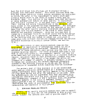 decisions regarding whether or not the proposed wastewater
treatment facility would provide adequate treatment and would
support a healthy aquatic community in the tailings impoundment
within a reasonable time-frame after mining/treatment operations
cease. These analysis methods included:
i. Simple box model treating the tailings pond as a
continuously stirred reactor with settling and leaching
as the important processes (Yearsley, 1992). This
model was used for estimating distributions of
suspended solids and certain metals in the water
column, only.
ii. One-dimensional (vertical), time-dependent model of the
tailings pond based on the WASP4 (Ambrose et al, 1991)
water quality simulation program. The application of
WASP4 to estimating distributions of suspended solids
and certain metals in the water column and sediments of
the proposed AJ Mine tailings pond is described .in
Yearsley (1993).
iii. Two-dimensional (longitudinal, vertical), time-
dependent model of the tailings pond water and sediment
quality based on the WASP4 (Ambrose et al, 1991) water
quality simulation program. The extension of the WASP4
methodology to two spatial dimensions was made for
purposes of determining how the location of the
discharge point affected the quality of the tailings
pond effluent.
iv. Two-dimensional (longitudinal, vertical), time-
dependent model of the tailings pond water quality
based on the CE-QUAL-W2 (Cole and Chapman, 1994)
computer model. CE-QUAL-W2 was included in the
analysis to supplement the WASP4 simulations by
incorporating a more accurate depiction of reservoir
hydrodynamics than could be provided by the WASP4
methodology.
The first two applications ((i.) and (ii.)) were based on
information provided in the FEIS, only. The results from (i.) and
(ii.) are documented elsewhere (Yearsley, 1992; Yearsley, 1993).
The primary objectives of these two applications were to provide
the basis for a more systematic review of water quality issues,
identify major processes affecting water quality in the proposed
tailings pond, and evaluate the sensitivity of results to
uncertainties in important parameters. It is often the case that
simple models and environmentally conservative assumptions will
be used to perform screening-level analyses of a complex problem
of this type. That has been EPA's approach with respect to the
28
image:
decisions regarding whether or not the proposed wastewater
treatment facility would provide adequate treatment and would
support a healthy aquatic community in the tailings impoundment
within a reasonable time-frame after mining/treatment operations
cease. These analysis methods included:
i. Simple box model treating the tailings pond as a
continuously stirred reactor with settling and leaching
as the important processes (Yearsley, 1992). This
model was used for estimating distributions of
suspended solids and certain metals in the water
column, only.
ii. One-dimensional (vertical), time-dependent model of the
tailings pond based on the WASP4 (Ambrose et al, 1991)
water quality simulation program. The application of
WASP4 to estimating distributions of suspended solids
and certain metals in the water column and sediments of
the proposed AJ Mine tailings pond is described .in
Yearsley (1993).
iii. Two-dimensional (longitudinal, vertical), time-
dependent model of the tailings pond water and sediment
quality based on the WASP4 (Ambrose et al, 1991) water
quality simulation program. The extension of the WASP4
methodology to two spatial dimensions was made for
purposes of determining how the location of the
discharge point affected the quality of the tailings
pond effluent.
iv. Two-dimensional (longitudinal, vertical), time-
dependent model of the tailings pond water quality
based on the CE-QUAL-W2 (Cole and Chapman, 1994)
computer model. CE-QUAL-W2 was included in the
analysis to supplement the WASP4 simulations by
incorporating a more accurate depiction of reservoir
hydrodynamics than could be provided by the WASP4
methodology.
The first two applications ((i.) and (ii.)) were based on
information provided in the FEIS, only. The results from (i.) and
(ii.) are documented elsewhere (Yearsley, 1992; Yearsley, 1993).
The primary objectives of these two applications were to provide
the basis for a more systematic review of water quality issues,
identify major processes affecting water quality in the proposed
tailings pond, and evaluate the sensitivity of results to
uncertainties in important parameters. It is often the case that
simple models and environmentally conservative assumptions will
be used to perform screening-level analyses of a complex problem
of this type. That has been EPA's approach with respect to the
28
image:
 proposed AJ tailings impoundment. The screening-level work set
the stage for subsequent, more sophisticated analyses.
Subsequent review of the first two analyses by independent
reviewers (Easton, Montgomery Watson) and by the applicant (Klone
Leonoff, 1993; Woodward'Clyde, 1993) led to a comprehensive
review of model parameters and, ultimately, the decision to apply
more sophisticated analysis methods in developing the TAR. The
more sophisticated methods are represented by the model
applications conducted in cases (iii.) and'(iv.). Case (iv.)
required data beyond that available in the FEIS.
Advanced mathematical modeling makes use of input data which
may be incomplete or have a high degree of variability or
uncertainty. Because of this, an important component of the
report is to characterize the degree of variability or
uncertainty in the available information.
3. WASP4 Conceptual Model
The toxic module (TOXIWASB) of EPA's Water Quality
Simulation Program (WASP version 4.32) was used to simulate the
levels of solids, cyanide and metals in the waters and sediments
of the proposed tailings pond during and after the operation of
the mine. The WASP software has been thoroughly tested and the
program has been used in a wide variety of applications. The
model kinetics in WASP generally reflect the current state of
knowledge for simulation of both inorganic and organic toxic
substances. The theoretical basis for the model and the user's
manual can be found in Ambrose et al (1991).
This application of WASP4 evolved from the work reported in
Yearsley (1993) . It represents an effort to characterize the
major processes affecting the distribution of solids and certain
metals in the tailings pond. These processes include turbulent
mixing processes associated in the pond itself, settling
characteristics of the tailings, leaching and partitioning*of
metals and effects of initial mixing associated with discharge.
It also represent a somewhat simplified approach, when compared
to the CE-QUAL-W2 simulations described later in this report.
This implementation of WASP4 is simplified in the sense that the
variability in environmental factors such as pond geometry,
inflow hydrology and local meteorology is not considered. Pond
geometry is idealized so as to capture the overall dimensions of
the tailings pond at Stage III (pond surface elevation
approximately 920 feet above Mean Sea Level) and the annual
average inflow hydrology of the Sheep Creek watershed. Effects
of local meteorology, particularly high winds are included
implicitly in other ways such as the coefficients of vertical
eddy diffusivity.
29
image:
proposed AJ tailings impoundment. The screening-level work set
the stage for subsequent, more sophisticated analyses.
Subsequent review of the first two analyses by independent
reviewers (Easton, Montgomery Watson) and by the applicant (Klone
Leonoff, 1993; Woodward'Clyde, 1993) led to a comprehensive
review of model parameters and, ultimately, the decision to apply
more sophisticated analysis methods in developing the TAR. The
more sophisticated methods are represented by the model
applications conducted in cases (iii.) and'(iv.). Case (iv.)
required data beyond that available in the FEIS.
Advanced mathematical modeling makes use of input data which
may be incomplete or have a high degree of variability or
uncertainty. Because of this, an important component of the
report is to characterize the degree of variability or
uncertainty in the available information.
3. WASP4 Conceptual Model
The toxic module (TOXIWASB) of EPA's Water Quality
Simulation Program (WASP version 4.32) was used to simulate the
levels of solids, cyanide and metals in the waters and sediments
of the proposed tailings pond during and after the operation of
the mine. The WASP software has been thoroughly tested and the
program has been used in a wide variety of applications. The
model kinetics in WASP generally reflect the current state of
knowledge for simulation of both inorganic and organic toxic
substances. The theoretical basis for the model and the user's
manual can be found in Ambrose et al (1991).
This application of WASP4 evolved from the work reported in
Yearsley (1993) . It represents an effort to characterize the
major processes affecting the distribution of solids and certain
metals in the tailings pond. These processes include turbulent
mixing processes associated in the pond itself, settling
characteristics of the tailings, leaching and partitioning*of
metals and effects of initial mixing associated with discharge.
It also represent a somewhat simplified approach, when compared
to the CE-QUAL-W2 simulations described later in this report.
This implementation of WASP4 is simplified in the sense that the
variability in environmental factors such as pond geometry,
inflow hydrology and local meteorology is not considered. Pond
geometry is idealized so as to capture the overall dimensions of
the tailings pond at Stage III (pond surface elevation
approximately 920 feet above Mean Sea Level) and the annual
average inflow hydrology of the Sheep Creek watershed. Effects
of local meteorology, particularly high winds are included
implicitly in other ways such as the coefficients of vertical
eddy diffusivity.
29
image:
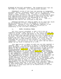 The major-difference between this application of WASP4 and
the previous•application (Yearsley, 1993) is in the treatment of
the tailings pond geometry. For this application, the waters of
the tailings impoundment have been conceptualized as a laterally
well-mixed system which is compartmentalized vertically and
horizontally into finite segments-, each with the same surface
area. Each of the segments is one meter in thickness, 350 meters
long and 600 meters wide (see Figure 4). The discharge of the
mine tailings is assumed to be distributed instantaneously over
one or more of the water column compartments depending on the
levels of available mixing energy. Once the tailings are
distributed in the water column the levels of solids and
associated dissolved and particulate concentrations of metals in
the water column are determined by the following processes:"
• Settling and resuspension rates of tailings solids
• Leaching rates of metals from tailings
• Partitioning between dissolved and adsorbed phases of
metals
• Longitudinal mixing in the tailings pond due to various
energy sources
• Vertical mixing in the tailings pond due to various energy
sources
• Rates of inflow of surface water and groundwater
• Rates of discharge from the impoundment
The speciation between dissolved and adsorbed phases of the
metals of interest are conceptualized in terms of the parent
material (tailings) and leaching products (Figure 5). The parent
material includes solids and associated metals. Two different
classes of solids, Sx and S2, are considered, each class
corresponding to a different median particle diameter. The
metals system, clf associated with the ith particle class (i=l,2)
of solids, Sif is transformed to the metals system, C2, toy
leaching only, where the systems C, and C2 are actually the same
metal (copper, for example). This is accomplished in the model
by using a partition coefficient which is large enough to prevent
the metals system, Clt from going into solution except by
leaching. The metals system, C2, undergoes repartitioning to
dissolved and adsorbed phases. The total concentration of the
metal in a given compartment is the sum of the adsorbed and
dissolved phases of Ct and C2.
The conceptual model includes a single sediment compartment
associated with each vertical segment of the reservoir (Figure
30
image:
The major-difference between this application of WASP4 and
the previous•application (Yearsley, 1993) is in the treatment of
the tailings pond geometry. For this application, the waters of
the tailings impoundment have been conceptualized as a laterally
well-mixed system which is compartmentalized vertically and
horizontally into finite segments-, each with the same surface
area. Each of the segments is one meter in thickness, 350 meters
long and 600 meters wide (see Figure 4). The discharge of the
mine tailings is assumed to be distributed instantaneously over
one or more of the water column compartments depending on the
levels of available mixing energy. Once the tailings are
distributed in the water column the levels of solids and
associated dissolved and particulate concentrations of metals in
the water column are determined by the following processes:"
• Settling and resuspension rates of tailings solids
• Leaching rates of metals from tailings
• Partitioning between dissolved and adsorbed phases of
metals
• Longitudinal mixing in the tailings pond due to various
energy sources
• Vertical mixing in the tailings pond due to various energy
sources
• Rates of inflow of surface water and groundwater
• Rates of discharge from the impoundment
The speciation between dissolved and adsorbed phases of the
metals of interest are conceptualized in terms of the parent
material (tailings) and leaching products (Figure 5). The parent
material includes solids and associated metals. Two different
classes of solids, Sx and S2, are considered, each class
corresponding to a different median particle diameter. The
metals system, clf associated with the ith particle class (i=l,2)
of solids, Sif is transformed to the metals system, C2, toy
leaching only, where the systems C, and C2 are actually the same
metal (copper, for example). This is accomplished in the model
by using a partition coefficient which is large enough to prevent
the metals system, Clt from going into solution except by
leaching. The metals system, C2, undergoes repartitioning to
dissolved and adsorbed phases. The total concentration of the
metal in a given compartment is the sum of the adsorbed and
dissolved phases of Ct and C2.
The conceptual model includes a single sediment compartment
associated with each vertical segment of the reservoir (Figure
30
image:
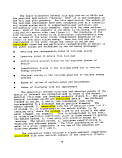 10
11
12
13
15
ie
17
18
19
20
H
22
23
24
25
26
27
29
30
31
32
33
36
37
38
39
40
41
43
44
45
46
47
48
50
51
52
53
54
55
Figure 4. Two-dimensonal grid used for WASP4 simulations of the
proposed AJ Mine tailings pond
image:
10
11
12
13
15
ie
17
18
19
20
H
22
23
24
25
26
27
29
30
31
32
33
36
37
38
39
40
41
43
44
45
46
47
48
50
51
52
53
54
55
Figure 4. Two-dimensonal grid used for WASP4 simulations of the
proposed AJ Mine tailings pond
image:
 Leaching
Adsorption
C - Chemical
S-Solid
Figure 5. Conceptual model of geochemical processes for
metals in the proposed AJ Mine tailings pond
image:
Leaching
Adsorption
C - Chemical
S-Solid
Figure 5. Conceptual model of geochemical processes for
metals in the proposed AJ Mine tailings pond
image:
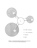 4) . Each of the sediment compartments has a variable volume
which can account for accumulation of solids settling out of the
tailings discharge. The sediment compartment also contains pore
water within which dissolved species of chemicals can occur.
Processes affecting levels of dissolved and adsorbed phases of
metals in these sediments are:
• Settling and resuspension rates of tailings solids
• Leaching rates of metals from tailings
• Partitioning between dissolved and adsorbed phases of
metals
• Vertical mixing in the tailings due to molecular diffusion
in the pore water
4. Time and Length Scales
The waters of the proposed tailings pond are conceptualized
as being comprised of a number of vertically and laterally well-
mixed compartments the size of the project, or with overall
length scales of 1000's of meters. The WASP 4 model formulation
will resolve laterally-averaged concentration differences at
scales of approximately the element size, which is one meter
vertically and 350 meters longitudinally. The length scales are
best professional estimates of what is needed to resolve details
of the problem associated with deposition, resuspension and
injection of the waste stream.
There are a number of time scales which may influence model
results. The simulation time period (time step) for the
numerical scheme used is of the order of minutes. The simulation
time period does have an effect on simulation accuracy, but the
fact that this time period is of the order of minutes does not
mean the model is simulating processes in the tailings pond at
this scale. The process time scales in the tailings pond and
sediments which can be resolved by the simulation are determined
by the rate of inflow of the waste stream, Sheep Creek and
groundwater; the amount of storage in the tailings pond; the
rates of vertical diffusion; the rate of leaching of the metals
from solid to dissolved; and the rates of settling and
resuspension.
jL-. Important Assumptions
Data from the FEIS and from other relevant sources were used
to implement the conceptual model within the WASP framework.
These sources provided the basis for defining important
parameters used in the simulations. The fixed parameter values
used in the simulations are given in Table 6. The implementation
of WASP for this problem included the following assumptions:
33
image:
4) . Each of the sediment compartments has a variable volume
which can account for accumulation of solids settling out of the
tailings discharge. The sediment compartment also contains pore
water within which dissolved species of chemicals can occur.
Processes affecting levels of dissolved and adsorbed phases of
metals in these sediments are:
• Settling and resuspension rates of tailings solids
• Leaching rates of metals from tailings
• Partitioning between dissolved and adsorbed phases of
metals
• Vertical mixing in the tailings due to molecular diffusion
in the pore water
4. Time and Length Scales
The waters of the proposed tailings pond are conceptualized
as being comprised of a number of vertically and laterally well-
mixed compartments the size of the project, or with overall
length scales of 1000's of meters. The WASP 4 model formulation
will resolve laterally-averaged concentration differences at
scales of approximately the element size, which is one meter
vertically and 350 meters longitudinally. The length scales are
best professional estimates of what is needed to resolve details
of the problem associated with deposition, resuspension and
injection of the waste stream.
There are a number of time scales which may influence model
results. The simulation time period (time step) for the
numerical scheme used is of the order of minutes. The simulation
time period does have an effect on simulation accuracy, but the
fact that this time period is of the order of minutes does not
mean the model is simulating processes in the tailings pond at
this scale. The process time scales in the tailings pond and
sediments which can be resolved by the simulation are determined
by the rate of inflow of the waste stream, Sheep Creek and
groundwater; the amount of storage in the tailings pond; the
rates of vertical diffusion; the rate of leaching of the metals
from solid to dissolved; and the rates of settling and
resuspension.
jL-. Important Assumptions
Data from the FEIS and from other relevant sources were used
to implement the conceptual model within the WASP framework.
These sources provided the basis for defining important
parameters used in the simulations. The fixed parameter values
used in the simulations are given in Table 6. The implementation
of WASP for this problem included the following assumptions:
33
image:
 Table 6. Important parameters and their values as used in the simulation
of suspended solids and total and dissolved metals in the proposed AJ
project tailings pond.
Parameter
Description
Value
Pt
Pf
Wt
Qavg
W2
Tailings density
Freshwater density
Dynamic viscosity of
freshwater
Tailings loading
Pond surface area
Average Sheep Creek
discharge
Settling rate of fine
tailings (2.5%)
Settling rate of coarse
tailings (97.5%)
2770kg/meter3
1000 kg/meter3
1.52xlO*3 kg/meter/second
2.36X10² kg/second
1.70xl06 meters2
1.382 meters3/second
l.SOxlO'6 meters/secon
l.OOxlO*4 meters/secon
Metals leaching rate 1.16xlO'7 seconds*1
image:
Table 6. Important parameters and their values as used in the simulation
of suspended solids and total and dissolved metals in the proposed AJ
project tailings pond.
Parameter
Description
Value
Pt
Pf
Wt
Qavg
W2
Tailings density
Freshwater density
Dynamic viscosity of
freshwater
Tailings loading
Pond surface area
Average Sheep Creek
discharge
Settling rate of fine
tailings (2.5%)
Settling rate of coarse
tailings (97.5%)
2770kg/meter3
1000 kg/meter3
1.52xlO*3 kg/meter/second
2.36X10² kg/second
1.70xl06 meters2
1.382 meters3/second
l.SOxlO'6 meters/secon
l.OOxlO*4 meters/secon
Metals leaching rate 1.16xlO'7 seconds*1
image:
 I The surface level of the tailings pond is constant and pond
size is approximately the same as the proposed tailings pond
at the end of the project (surface level at 918 feet above
Mean Sea Level)
• Settling rates of particles are determined from Stokes1
Law
• The tailings slurry is made up of two particle classes, the
first class comprising a very small fraction of the
discharge which goes into suspension when the tailings are
initially discharged, the second comprising the remainder of
the discharge which settles out almost immediately. The
particle size of each fraction is assumed to be equal to the
particle size of the median fraction for each group.
• Settling velocities for each of the two particle classes can
be estimated from Stokes1 Law using the median diameter for
each fraction, or the lowest reported value, in cases, where
the particle size of any fraction was not given in any
reports provided by the applicant.
• Leaching rates of metals from solid to dissolved are
characterized by first-order reactions
• Solubility of metals in freshwater is determined by ratios
of dissolved to total metals analyzed by Frank (1994)
• Inflow rate to and discharge rate from the impoundment are
both constant and equal to the annual average flow of Sheep
Creek
• Dissolved levels of metals in Sheep Creek are below
detection limits
£._ Parameter Estimation
The density of the tailings, pt, was obtained from results
reported by Knight and Piesold (1989). The leaching rate, KL,
was chosen so as to have a time scale (100 days) approximately
the same as the time scale found in the bench tests for iron, as
presented in Appendix A of the FEIS. Shorter time scales for the
leaching rate would result in higher concentrations of dissolved
metals in the tailings pond.
The fraction of important metals in the digested slurry, for
both solid and dissolved phases, were estimated from various data
sources by Frank (1994). These estimates are given in Table 7.
Partitioning coefficients for determining the equilibrium
concentrations of metals in the solid and dissolved phases were
35
image:
I The surface level of the tailings pond is constant and pond
size is approximately the same as the proposed tailings pond
at the end of the project (surface level at 918 feet above
Mean Sea Level)
• Settling rates of particles are determined from Stokes1
Law
• The tailings slurry is made up of two particle classes, the
first class comprising a very small fraction of the
discharge which goes into suspension when the tailings are
initially discharged, the second comprising the remainder of
the discharge which settles out almost immediately. The
particle size of each fraction is assumed to be equal to the
particle size of the median fraction for each group.
• Settling velocities for each of the two particle classes can
be estimated from Stokes1 Law using the median diameter for
each fraction, or the lowest reported value, in cases, where
the particle size of any fraction was not given in any
reports provided by the applicant.
• Leaching rates of metals from solid to dissolved are
characterized by first-order reactions
• Solubility of metals in freshwater is determined by ratios
of dissolved to total metals analyzed by Frank (1994)
• Inflow rate to and discharge rate from the impoundment are
both constant and equal to the annual average flow of Sheep
Creek
• Dissolved levels of metals in Sheep Creek are below
detection limits
£._ Parameter Estimation
The density of the tailings, pt, was obtained from results
reported by Knight and Piesold (1989). The leaching rate, KL,
was chosen so as to have a time scale (100 days) approximately
the same as the time scale found in the bench tests for iron, as
presented in Appendix A of the FEIS. Shorter time scales for the
leaching rate would result in higher concentrations of dissolved
metals in the tailings pond.
The fraction of important metals in the digested slurry, for
both solid and dissolved phases, were estimated from various data
sources by Frank (1994). These estimates are given in Table 7.
Partitioning coefficients for determining the equilibrium
concentrations of metals in the solid and dissolved phases were
35
image:
 estimated from -the ratios given in Table 7 using the following
equation:
where, p
Kp= linear partition coefficient, I/kg
csoiid = concentration of constituent in solid phase,
mg/1
Cdiss= concentration of constituent in dissolved phase,
mg/1
TSS= concentration of total suspended solids, mg/1
a. Vertical Mixing
Rates of vertical diffusion in the tailings pond were
determined by the levels of available turbulent energy.
According to the FEIS, the potential sources of this energy
include wind stress, kinetic energy from advective sources
including Sheep Creek and the waste stream itself and kinetic
energy associated with avalanches. The FEIS (page 4-34) gives
estimates of the coefficient of turbulent diffusion for
stratified reservoirs as 1.00x10"* meters2/second and for
unstratified reservoirs as l.OOxlO"3 meters2/second. The FEIS
states
"A sense of how much settling would occur can be gained by
estimating a vertical diffusion time scale for the
impoundment, and comparing it to the settling velocity of
discrete particles. A maximum diffusivity value of D=0.0001
m2/sec has been suggested for prediction of hypolimnetic
diffusion in stratified reservoirs (Imberger and Patterson
1981; Harleman 1986).
However, available data suggest that the impoundment would
likely be unstratified, and vertical diffusivity would
likely be much greater. Assuming a vertical diffusivity of
D=0.001 m2/sec. leads to a characteristic time scale of
approximately one day. "
In Woodward-Clyde's (1993) evaluation of the WASP4 analysis
done by Yearsley (1993), coefficients of vertical eddy
diffusivity ranged between IxlO'6 and IxlO'4 meters2/second. The
applicant asserted (Bergstrom, 1993) that for the WASP4 analysis
of the tailings, "l.OxlO'0* meters2/second would characterize the
36
image:
estimated from -the ratios given in Table 7 using the following
equation:
where, p
Kp= linear partition coefficient, I/kg
csoiid = concentration of constituent in solid phase,
mg/1
Cdiss= concentration of constituent in dissolved phase,
mg/1
TSS= concentration of total suspended solids, mg/1
a. Vertical Mixing
Rates of vertical diffusion in the tailings pond were
determined by the levels of available turbulent energy.
According to the FEIS, the potential sources of this energy
include wind stress, kinetic energy from advective sources
including Sheep Creek and the waste stream itself and kinetic
energy associated with avalanches. The FEIS (page 4-34) gives
estimates of the coefficient of turbulent diffusion for
stratified reservoirs as 1.00x10"* meters2/second and for
unstratified reservoirs as l.OOxlO"3 meters2/second. The FEIS
states
"A sense of how much settling would occur can be gained by
estimating a vertical diffusion time scale for the
impoundment, and comparing it to the settling velocity of
discrete particles. A maximum diffusivity value of D=0.0001
m2/sec has been suggested for prediction of hypolimnetic
diffusion in stratified reservoirs (Imberger and Patterson
1981; Harleman 1986).
However, available data suggest that the impoundment would
likely be unstratified, and vertical diffusivity would
likely be much greater. Assuming a vertical diffusivity of
D=0.001 m2/sec. leads to a characteristic time scale of
approximately one day. "
In Woodward-Clyde's (1993) evaluation of the WASP4 analysis
done by Yearsley (1993), coefficients of vertical eddy
diffusivity ranged between IxlO'6 and IxlO'4 meters2/second. The
applicant asserted (Bergstrom, 1993) that for the WASP4 analysis
of the tailings, "l.OxlO'0* meters2/second would characterize the
36
image:
 Table 7 Estimated solid and dissolved concentrations of certain metals in
the waste stream discharged from the proposed AJ Mine milling process.
Estimates of concentrations are derived from Section VI.D.
Metal
Arsenic
Cadmium
Chromium
Total CN
Copper
Lead
Mercury
Selenium
Zinc
Concentration
Solid
(mg/kg)
9.8
11.0
35.0
0.0
260.
200.
0.27
1.
530
Dissolved
(mg/1)
0.014
0.010
0.020
2.5
1.300
0.020
0.005
0.016
0.087
image:
Table 7 Estimated solid and dissolved concentrations of certain metals in
the waste stream discharged from the proposed AJ Mine milling process.
Estimates of concentrations are derived from Section VI.D.
Metal
Arsenic
Cadmium
Chromium
Total CN
Copper
Lead
Mercury
Selenium
Zinc
Concentration
Solid
(mg/kg)
9.8
11.0
35.0
0.0
260.
200.
0.27
1.
530
Dissolved
(mg/1)
0.014
0.010
0.020
2.5
1.300
0.020
0.005
0.016
0.087
image:
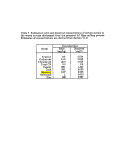 most conservative of high wind conditions, not characteristic of
typical situations, and that l.OxlO'05 would be characteristic of
general pond conditions". The range chosen for the coefficient
of vertical eddy diffusivity in these simulations corresponds to
the ranges described by Bergstrom (1993).
These coefficients are measures of the general levels of
vertical mixing processes in reservoirs. For the purposes of
this report, it has been assumed that, levels of energy implied by
these coefficients do not include energy sources unique to this
project such as avalanches and energy transport in the waste
stream itself. The energy associated with the waste stream must
be dissipated in some way and this can happen by enhancing
vertical mixing processes or by scouring sediment from the
bottom. Data collected by Rescan Environmental Services Ltd
(1983) in the vicinity of the Island Copper discharge show that
vertical mixing associated with discharge of mine tailings can
lead to high levels of suspended solids (Figures 6 and 7) in the
water column.
b. Pore Water Diffusion-Rates
Flux of dissolved metals from the sediment pore water to the
overlying water column is of concern for water quality conditions
in the tailings pond after the mining operation has ceased. This
flux is determined by the geochemical processes which affect
partitioning between solid and dissolved phases in the sediments
as well as the rates of advection and diffusion within the pore
water. Rates of advection are determined primarily by
groundwater flow, which are discussed in a later section of this
report. Diffusion rates within the pore water are generally at
levels comparable to molecular diffusion (Schnoor et al., 1987).
However, Schnoor et al. (1987) point out that bioturbation of the
sediments by benthic fauna or fish can increase diffusion rates
from the pore water to the overlying water by an order of
magnitude. The metals concentrations in the pore water represent
a serious threat to water quality in the proposed tailings pond
after the mining operation is finished. To .assess the effects of
changes in the rate of diffusion from the pore water on the
overlying water column, the pore water diffusion coefficient was
varied between the molecular diffusion rate (l.OxlO-9
meters2/second) and the diffusion rate for sediments subject to
bioturbation (l.OxlO"8 metersz/second) .
c. Initial Mixing of Discharge
The FEIS (page 4-34) states that no methods of analysis are
available to describe the initial mixing of the waste stream in
the tailings pond. This is not entirely the case, as a model of
the density flow for the proposed Quartz Hill project was used to
estimate the plume characteristics of a discharge approximately
38
image:
most conservative of high wind conditions, not characteristic of
typical situations, and that l.OxlO'05 would be characteristic of
general pond conditions". The range chosen for the coefficient
of vertical eddy diffusivity in these simulations corresponds to
the ranges described by Bergstrom (1993).
These coefficients are measures of the general levels of
vertical mixing processes in reservoirs. For the purposes of
this report, it has been assumed that, levels of energy implied by
these coefficients do not include energy sources unique to this
project such as avalanches and energy transport in the waste
stream itself. The energy associated with the waste stream must
be dissipated in some way and this can happen by enhancing
vertical mixing processes or by scouring sediment from the
bottom. Data collected by Rescan Environmental Services Ltd
(1983) in the vicinity of the Island Copper discharge show that
vertical mixing associated with discharge of mine tailings can
lead to high levels of suspended solids (Figures 6 and 7) in the
water column.
b. Pore Water Diffusion-Rates
Flux of dissolved metals from the sediment pore water to the
overlying water column is of concern for water quality conditions
in the tailings pond after the mining operation has ceased. This
flux is determined by the geochemical processes which affect
partitioning between solid and dissolved phases in the sediments
as well as the rates of advection and diffusion within the pore
water. Rates of advection are determined primarily by
groundwater flow, which are discussed in a later section of this
report. Diffusion rates within the pore water are generally at
levels comparable to molecular diffusion (Schnoor et al., 1987).
However, Schnoor et al. (1987) point out that bioturbation of the
sediments by benthic fauna or fish can increase diffusion rates
from the pore water to the overlying water by an order of
magnitude. The metals concentrations in the pore water represent
a serious threat to water quality in the proposed tailings pond
after the mining operation is finished. To .assess the effects of
changes in the rate of diffusion from the pore water on the
overlying water column, the pore water diffusion coefficient was
varied between the molecular diffusion rate (l.OxlO-9
meters2/second) and the diffusion rate for sediments subject to
bioturbation (l.OxlO"8 metersz/second) .
c. Initial Mixing of Discharge
The FEIS (page 4-34) states that no methods of analysis are
available to describe the initial mixing of the waste stream in
the tailings pond. This is not entirely the case, as a model of
the density flow for the proposed Quartz Hill project was used to
estimate the plume characteristics of a discharge approximately
38
image:
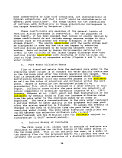 Figure 6. Suspended solids 300 meters
from, the TslanH Copper discharge
(Rescan, 1983)
(40)-
(50)-
(60)-
(70)-
(80)
0 500 1000 1500 2000 2500
Suspended Solids • mg/1
image:
Figure 6. Suspended solids 300 meters
from, the TslanH Copper discharge
(Rescan, 1983)
(40)-
(50)-
(60)-
(70)-
(80)
0 500 1000 1500 2000 2500
Suspended Solids • mg/1
image:
 Figure 7. Suspended solids in Rupert Inlet
1200 meters from, the Island Copper discharge
(Rescan, 1983)
(30)
800
Suspended Solids • rag/I
image:
Figure 7. Suspended solids in Rupert Inlet
1200 meters from, the Island Copper discharge
(Rescan, 1983)
(30)
800
Suspended Solids • rag/I
image:
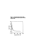 three times lar-ger than the proposed AJ Mine discharge (Kowalik
and Findikakis, 1985) . The ocean disposal model of Koh and Chang
(1973) which evolved into the Offshore Operators Committee
drilling mud model (Brandsma et al, 1983) also provides a
framework for examining density flows such as that associated
with the proposed AJ Mine project. However, at the time the
modeling process was begun by EPA Region 10, the only information
available for evaluating the initial mixing characteristics of
the discharge was limited to that provided in the FEIS. The
analysis of initial mixing of the AJ Mine tailings discharge, as
provided in the FEIS, was not sufficiently quantitative to
provide inputs for simulation methods such as WASP4. The initial
approach used to address this question was to survey the
available literature; primarily that associated with the
discharge of drilling muds and cutting from offshore drilling
operations (Ayers et al, 1982, for example) as well as the
discharge of tailings from other mining operations such Island
Copper on Vancouver Island. In these studies, field data showed
that 5-10% of the total load became suspended during the initial
discharge phase.
• t
The WASP4 simulations reported by Yearsley (1993) were based
on initial mixing characteristics approximately the same as those
described by Schubel et al (1978) for dredge materials, Brandsma
et al (19783) for drilling muds discharges and from the
evaluation of the tailings discharge at the Island Copper Mine on
Vancouver Island. Assumptions regarding the initial mixing
characteristics of the proposed discharge were reviewed by
various consultants for the applicant and by a number of experts
in the field of sediment transport. As a result of this review,
EPA Region 10, in cooperation with Echo Bay, convened an ad hoc
panel of experts to develop a best professional estimate of the
characteristics of the initial discharge. Their recommendations
are- described, in part, below:
Mark Dortch, PhD, US Army Corps of Engineers, Waterways
Experiment Station (1993):
I recommend a mid-range compromise value of 2.5 percent,
which should still be on the conservative side. The 625
tons/day of suspension should be composed of particles from the 0
to 2 5 percent smallest size class, i.e., 97.5% of the particles
by weight is (sic) larger than this class. Therefore, a median
diameter corresponding to the 1.25 percentile should be used
Earl Hayter, PhD, Clemson University, South Carolina Water
Resources Research Institute (1993):
"--Based on the tailings size gradation, settling velocity
analysis, and characteristics (e.g., specific gravity,
mineralogy) of the tailings, my estimate is io<
41
image:
three times lar-ger than the proposed AJ Mine discharge (Kowalik
and Findikakis, 1985) . The ocean disposal model of Koh and Chang
(1973) which evolved into the Offshore Operators Committee
drilling mud model (Brandsma et al, 1983) also provides a
framework for examining density flows such as that associated
with the proposed AJ Mine project. However, at the time the
modeling process was begun by EPA Region 10, the only information
available for evaluating the initial mixing characteristics of
the discharge was limited to that provided in the FEIS. The
analysis of initial mixing of the AJ Mine tailings discharge, as
provided in the FEIS, was not sufficiently quantitative to
provide inputs for simulation methods such as WASP4. The initial
approach used to address this question was to survey the
available literature; primarily that associated with the
discharge of drilling muds and cutting from offshore drilling
operations (Ayers et al, 1982, for example) as well as the
discharge of tailings from other mining operations such Island
Copper on Vancouver Island. In these studies, field data showed
that 5-10% of the total load became suspended during the initial
discharge phase.
• t
The WASP4 simulations reported by Yearsley (1993) were based
on initial mixing characteristics approximately the same as those
described by Schubel et al (1978) for dredge materials, Brandsma
et al (19783) for drilling muds discharges and from the
evaluation of the tailings discharge at the Island Copper Mine on
Vancouver Island. Assumptions regarding the initial mixing
characteristics of the proposed discharge were reviewed by
various consultants for the applicant and by a number of experts
in the field of sediment transport. As a result of this review,
EPA Region 10, in cooperation with Echo Bay, convened an ad hoc
panel of experts to develop a best professional estimate of the
characteristics of the initial discharge. Their recommendations
are- described, in part, below:
Mark Dortch, PhD, US Army Corps of Engineers, Waterways
Experiment Station (1993):
I recommend a mid-range compromise value of 2.5 percent,
which should still be on the conservative side. The 625
tons/day of suspension should be composed of particles from the 0
to 2 5 percent smallest size class, i.e., 97.5% of the particles
by weight is (sic) larger than this class. Therefore, a median
diameter corresponding to the 1.25 percentile should be used
Earl Hayter, PhD, Clemson University, South Carolina Water
Resources Research Institute (1993):
"--Based on the tailings size gradation, settling velocity
analysis, and characteristics (e.g., specific gravity,
mineralogy) of the tailings, my estimate is io<
41
image:
 Ray B. Krone, PhD, Ray B. Krone & Associates (1993):
ii—j would expect an upper limit of less than 3 percent of the
total load of lowest decile particles and 2 percent of the second
decile. In view of the dissimilarity between the finer sediments
in the referred dredging studies and the proposed mine tailings,
these estimates are probably high. "
Based on these recommendations, the WASP4 simulations were
performed assuming that 2.5% of the total load, comprising
particles from the 0 to 2.5 percent smallest size class, were
suspended initially at the discharge point and that the remainder
(97.5%) settled quickly to the bottom of the tailings pond. The
discharge was assumed to be distributed uniformly throughout the
bottom element of the conceptualized two-dimensional grid,
simulating a discharge confined to the bottom.
d. Settling, Deposition and Resuspension
Sediment transport mechanisms will play an important part in
determining levels of suspended- solids and metals in the tailings
pond. Primary transport mechanisms which must be considered are
settling, deposition and resuspension. While a great deal of
research has been devoted to investigating mechanisms of sediment
transport, there is still much uncertainty in quantifying these
mechanisms. Information in the FEIS specific to this project is
limited to a series of settling tests performed by Lakefield
Research (1990). However, these tests were not designed to
estimate settling velocities of particle classes.
Recently, Hartman Associates (1994) conducted tests on the
mine tailings using the U.S. Army Corps of Engineers SETTLE
methodology. Krone (1994), however, observed that the results of
these particular tests could not be applied directly to
estimating settling velocities of particle classes and
recommended additional tests. The results of the additional
tests recommended by Krone (1994) were not available at the time
the modeling work described below was performed. Nor was it
clear that these tests would address all the issues of
uncertainty associated with the settling, deposition and
resuspension of material in the proposed AJ Mine tailings pond.
As a result, the WASP4 simulations do not include any of the test
results. However, as described later in this report, a
preliminary examination of these data was performed using CE-
QUAL-W2.
Because of the limited information provided in the FEIS and
by the applicant, it was, therefore, necessary to rely on the
judgment of sediment transfer experts to provide input for the
WASP4 simulations. None of the experts made specific
recommendations regarding ways of computing the settling
velocity, although Krone (1993) observed that "Absence of
42
image:
Ray B. Krone, PhD, Ray B. Krone & Associates (1993):
ii—j would expect an upper limit of less than 3 percent of the
total load of lowest decile particles and 2 percent of the second
decile. In view of the dissimilarity between the finer sediments
in the referred dredging studies and the proposed mine tailings,
these estimates are probably high. "
Based on these recommendations, the WASP4 simulations were
performed assuming that 2.5% of the total load, comprising
particles from the 0 to 2.5 percent smallest size class, were
suspended initially at the discharge point and that the remainder
(97.5%) settled quickly to the bottom of the tailings pond. The
discharge was assumed to be distributed uniformly throughout the
bottom element of the conceptualized two-dimensional grid,
simulating a discharge confined to the bottom.
d. Settling, Deposition and Resuspension
Sediment transport mechanisms will play an important part in
determining levels of suspended- solids and metals in the tailings
pond. Primary transport mechanisms which must be considered are
settling, deposition and resuspension. While a great deal of
research has been devoted to investigating mechanisms of sediment
transport, there is still much uncertainty in quantifying these
mechanisms. Information in the FEIS specific to this project is
limited to a series of settling tests performed by Lakefield
Research (1990). However, these tests were not designed to
estimate settling velocities of particle classes.
Recently, Hartman Associates (1994) conducted tests on the
mine tailings using the U.S. Army Corps of Engineers SETTLE
methodology. Krone (1994), however, observed that the results of
these particular tests could not be applied directly to
estimating settling velocities of particle classes and
recommended additional tests. The results of the additional
tests recommended by Krone (1994) were not available at the time
the modeling work described below was performed. Nor was it
clear that these tests would address all the issues of
uncertainty associated with the settling, deposition and
resuspension of material in the proposed AJ Mine tailings pond.
As a result, the WASP4 simulations do not include any of the test
results. However, as described later in this report, a
preliminary examination of these data was performed using CE-
QUAL-W2.
Because of the limited information provided in the FEIS and
by the applicant, it was, therefore, necessary to rely on the
judgment of sediment transfer experts to provide input for the
WASP4 simulations. None of the experts made specific
recommendations regarding ways of computing the settling
velocity, although Krone (1993) observed that "Absence of
42
image:
 cohesion is assumed by the modelers, a conservative assumption."
Given the lack of consensus from the panel, it was assumed that
Stokes1 Law settling was appropriate for this analysis.
Determination of settling velocities using Stokes1 Law
requires that a characteristic particle size be specified.
Dortch (1993), as quoted above, is the .most specific in regard to
estimating particle sizes. Dortch (1993) recommended the use of
the particle size associated with the 1.25 percentile. However,
the tests on tailings characteristics performed by Knight and
Piesold (1989) provide results which include particles associated
with the 5.9 percentile, but no lower. Rather than extrapolate
the Knight and Piesold (1989) results to the 1.25 percentile, the
5.9 percentile particle size diameter was chosen to represent the
settling velocity of those particles which become suspended
during initial discharge. As pointed out by Dortch (1993), this
would lead to lower simulated levels of suspended material than
if the true median diameter were used to estimate particle fall
velocity.
According to the WASP4 manual (Ambrose et al, 1991) the
probability of deposition depends on the shear stress on the
benthic surface and the suspended sediment size and cohesiveness.
For fine silts of 5 microns, or less, the manual states that
deposition is not to be expected, even under quiescent
conditions. Ariathurai (1985) presents results of Hjulstrom
which show regions of erosion-transportation-sedimentation in
the space characterized by mean velocity near the bed and
particle diameter. These results show that particles of 100
microns or less remain in suspension at very low velocities
(<0.001 meters/second). The FEIS gives a semi-quantitative
discussion of resuspension of tailings pond sediments (page 4-34)
as they are affected by cyclic changes in inflow-outflow
characteristics and as a result of high winds. The panel of
experts had a wide range of recommendations regarding actual
values. This included values of the probability of deposition as
low as 0.2 and as high as 1.0. Previous simulations using WASP4
(Yearsley, 1993) considering values as low as 0.2, also.
However, for the simulations performed here,'the probability of
deposition was assumed to be 1.0 for all conditions. A lower
probablility of deposition would result in higher concentrations
of simulated suspended solids.
e. Geochemical Processes
Partitioning between dissolved and adsorbed phases will
determine the importance of sediment transport in the mass
balance of metals. The FEIS does provide the results of several
leach column tests and these tests provide the basis for the
estimate of first-order rate of leaching from solid to dissolved.
The leaching rate used in the various scenarios was chosen so as
to have a time scale (100 days) approximately the same as the
43
image:
cohesion is assumed by the modelers, a conservative assumption."
Given the lack of consensus from the panel, it was assumed that
Stokes1 Law settling was appropriate for this analysis.
Determination of settling velocities using Stokes1 Law
requires that a characteristic particle size be specified.
Dortch (1993), as quoted above, is the .most specific in regard to
estimating particle sizes. Dortch (1993) recommended the use of
the particle size associated with the 1.25 percentile. However,
the tests on tailings characteristics performed by Knight and
Piesold (1989) provide results which include particles associated
with the 5.9 percentile, but no lower. Rather than extrapolate
the Knight and Piesold (1989) results to the 1.25 percentile, the
5.9 percentile particle size diameter was chosen to represent the
settling velocity of those particles which become suspended
during initial discharge. As pointed out by Dortch (1993), this
would lead to lower simulated levels of suspended material than
if the true median diameter were used to estimate particle fall
velocity.
According to the WASP4 manual (Ambrose et al, 1991) the
probability of deposition depends on the shear stress on the
benthic surface and the suspended sediment size and cohesiveness.
For fine silts of 5 microns, or less, the manual states that
deposition is not to be expected, even under quiescent
conditions. Ariathurai (1985) presents results of Hjulstrom
which show regions of erosion-transportation-sedimentation in
the space characterized by mean velocity near the bed and
particle diameter. These results show that particles of 100
microns or less remain in suspension at very low velocities
(<0.001 meters/second). The FEIS gives a semi-quantitative
discussion of resuspension of tailings pond sediments (page 4-34)
as they are affected by cyclic changes in inflow-outflow
characteristics and as a result of high winds. The panel of
experts had a wide range of recommendations regarding actual
values. This included values of the probability of deposition as
low as 0.2 and as high as 1.0. Previous simulations using WASP4
(Yearsley, 1993) considering values as low as 0.2, also.
However, for the simulations performed here,'the probability of
deposition was assumed to be 1.0 for all conditions. A lower
probablility of deposition would result in higher concentrations
of simulated suspended solids.
e. Geochemical Processes
Partitioning between dissolved and adsorbed phases will
determine the importance of sediment transport in the mass
balance of metals. The FEIS does provide the results of several
leach column tests and these tests provide the basis for the
estimate of first-order rate of leaching from solid to dissolved.
The leaching rate used in the various scenarios was chosen so as
to have a time scale (100 days) approximately the same as the
43
image:
 time scale found in the bench tests for iron as present in
Appendix A, Volume II of the FEIS. The partition coefficient,
KPI for each of the metals was estimated based on the ratio of
total and dissolved concentrations listed in Table 7. The
results for the equilibrium partition coefficients are given in
Table 8.
f. Groundwater Flow
The FEIS (Dept. of Interior, 1992) estimated that
groundwater flow was 24% of the total discharge at the "narrows".
SRK (1994) estimated that the present level of groundwater flow
to Sheep Creek is about 7 cfs. Although the SRK (1994) report is
not specific regarding the source of the groundwater, others
(Easton, 1993) have suggested it is probably associated with the
alluvium covering the floor of Sheep Creek valley to thicknesses
of as much as twenty feet (SRK, 1990). Groundwater flow in the
igneous rocks beneath and surrounding Sheep Creek valley is
estimated to be low. The previous application of WASP4
(Yearsley, 1993) considered the effects of groundwater flow,
based on flow estimates given ±n the FEIS. Most of those who
reviewed the previous WASP4 simulations or had visited Sheep
Creek valley (Easton, 1993; Krone, 1994) felt that groundwater
return to Sheep Creek would not be a factor once the tailings had
been deposited. However, these are opinions, only, and have not
included any quantitative assessment of:
(1) the relative transmissivity of alluvium, talus, basement
rock and tailings. Data submitted by the applicant (SRK,
1990) show the extent of alluvium and talus, both of
which have relatively high transmissivity compared to the
basement rock;
(2) the piezometric head of the groundwater system;
(3) the rate of groundwater flow through the existing system
of mine tunnels.
A preliminary analysis of groundwater is given in Appendix
C. The preliminary analysis described in Appendix C supports the
hypothesis that groundwater will flow through the tailings into
the tailings pond. However, the analysis is based on very
limited data. Until these issues are specifically addressed,
impacts of the groundwater cannot be ignored, particularly as it
could potentially affect water quality after mining has ended and
the tailings pond reverts to waters of the United States. For
purposes of quantifying this potential, some simulations were
performed assuming a groundwater flow of 7 cfs, as assumed by SRK
(1994).
44
image:
time scale found in the bench tests for iron as present in
Appendix A, Volume II of the FEIS. The partition coefficient,
KPI for each of the metals was estimated based on the ratio of
total and dissolved concentrations listed in Table 7. The
results for the equilibrium partition coefficients are given in
Table 8.
f. Groundwater Flow
The FEIS (Dept. of Interior, 1992) estimated that
groundwater flow was 24% of the total discharge at the "narrows".
SRK (1994) estimated that the present level of groundwater flow
to Sheep Creek is about 7 cfs. Although the SRK (1994) report is
not specific regarding the source of the groundwater, others
(Easton, 1993) have suggested it is probably associated with the
alluvium covering the floor of Sheep Creek valley to thicknesses
of as much as twenty feet (SRK, 1990). Groundwater flow in the
igneous rocks beneath and surrounding Sheep Creek valley is
estimated to be low. The previous application of WASP4
(Yearsley, 1993) considered the effects of groundwater flow,
based on flow estimates given ±n the FEIS. Most of those who
reviewed the previous WASP4 simulations or had visited Sheep
Creek valley (Easton, 1993; Krone, 1994) felt that groundwater
return to Sheep Creek would not be a factor once the tailings had
been deposited. However, these are opinions, only, and have not
included any quantitative assessment of:
(1) the relative transmissivity of alluvium, talus, basement
rock and tailings. Data submitted by the applicant (SRK,
1990) show the extent of alluvium and talus, both of
which have relatively high transmissivity compared to the
basement rock;
(2) the piezometric head of the groundwater system;
(3) the rate of groundwater flow through the existing system
of mine tunnels.
A preliminary analysis of groundwater is given in Appendix
C. The preliminary analysis described in Appendix C supports the
hypothesis that groundwater will flow through the tailings into
the tailings pond. However, the analysis is based on very
limited data. Until these issues are specifically addressed,
impacts of the groundwater cannot be ignored, particularly as it
could potentially affect water quality after mining has ended and
the tailings pond reverts to waters of the United States. For
purposes of quantifying this potential, some simulations were
performed assuming a groundwater flow of 7 cfs, as assumed by SRK
(1994).
44
image:
 Table 8. Equilibrium partition coefficients, Kp, for various metals in the proposed
AJ Mine tailings discharge, computed using data provided by the applicant.
Coefficients computed from the data are compared to estimates given in
Mills et al (1985)
Element
Arsenic
Cadmim
Chromium
Copoper
Mercury
Lead
oeienium
Zinc
FEIS Digest
(mg/kg)
9.8
1.1
35
260
0.27
200
1
X
530
Decant
(mg/1)
0.014
0.010
0.020
1.300
0.005
0.020
nniA
U.UJ.O
0.087
Total Solids
(kg/I)
0.637
0.637
0.637
0.637
0.637
0.637
Ofl^7
.DO/
0.637
Total
(mg/l)
6.26
7.02
22.3
167.
0.18
127.
Ofifi
.DO
338.
Kp
(data)
(l/ke)
700
1100
- 1750
200
54
10000
eft
6100
Kp
(Mills et al,1985)
(I/kg)
278
16
59000
17
0.3
1700
380
image:
Table 8. Equilibrium partition coefficients, Kp, for various metals in the proposed
AJ Mine tailings discharge, computed using data provided by the applicant.
Coefficients computed from the data are compared to estimates given in
Mills et al (1985)
Element
Arsenic
Cadmim
Chromium
Copoper
Mercury
Lead
oeienium
Zinc
FEIS Digest
(mg/kg)
9.8
1.1
35
260
0.27
200
1
X
530
Decant
(mg/1)
0.014
0.010
0.020
1.300
0.005
0.020
nniA
U.UJ.O
0.087
Total Solids
(kg/I)
0.637
0.637
0.637
0.637
0.637
0.637
Ofl^7
.DO/
0.637
Total
(mg/l)
6.26
7.02
22.3
167.
0.18
127.
Ofifi
.DO
338.
Kp
(data)
(l/ke)
700
1100
- 1750
200
54
10000
eft
6100
Kp
(Mills et al,1985)
(I/kg)
278
16
59000
17
0.3
1700
380
image:
 g. Avalanches
The previous simulations using WASP4 (Yearsley, 1993)
considered the potential impacts of avalanches on water quality,
primarily as they might affect levels of suspended solids. The'
simulations were based on the FEIS estimates of a maximum
probable energy of 107 joules (page 4-33) for a single event.
This kinetic energy was converted into potential energy by
assuming the effect of the avalanche was to resuspend tailings
deposited on the bottom of the pond during 'operation of the mine.
The tailings disturbed by the avalanche were distributed
uniformly throughout the pond, with the center of gravity of this
mass of material at a distance equal to half the depth of the
reservoir above the bottom of the pond, It was further assumed
that the process was 100% efficient in converting the kinetic
energy to potential energy.
One reviewer of this avalanche analysis felt that avalanche
energy could well be orders of magnitude higher, while the
applicant believes that the avalanche issue has been resolved
based on work reported by Hears (1993). The range of uncertainty
associated with this question was substantially greater than for
any of the others. Until this uncertainty can be reduced to a
level commensurate with other issues, the avalanche issue should
be considered qualitatively as an additional risk factor, but one
which will not be included in WASP4 simulations.
h. Reservoir Hydrodynamics
WASP4 is constructed as a framework for performing mass
balances of heavy metals and other toxic substances. It does not
simulate the hydrodynamics of surface or groundwater systems.
Rather, it relies on reservoir hydrodynamic results being
supplied externally by other methods of analysis. For the
simulations described in this report, three different modes of
reservoir hydrodynamics were considered. These modes were
formulated to capture flow characteristics which have been
observed in other reservoir systems or were suggested as possible
outcomes by those who reviewed the previous application of WASP4
to the AJ Mine tailings pond. The three modes of reservoir
hydrodynamics were 1) surface flow; 2) uniform flow; and 3)
underflow. In the first mode, the inflow from Sheep Creek is
confined to the surface two meters (Figure 8) , much as in the
analysis done by Woodward-Clyde (1993). In the second mode, the
inflow is distributed uniformly from top to bottom (Figure 9) and
in the third mode, the inflow is confined to the bottom two
meters (Figure 10). In all cases, inflow and outflow are assumed
to be constant and equal to the annual average flow of Sheep
Creek.
46
image:
g. Avalanches
The previous simulations using WASP4 (Yearsley, 1993)
considered the potential impacts of avalanches on water quality,
primarily as they might affect levels of suspended solids. The'
simulations were based on the FEIS estimates of a maximum
probable energy of 107 joules (page 4-33) for a single event.
This kinetic energy was converted into potential energy by
assuming the effect of the avalanche was to resuspend tailings
deposited on the bottom of the pond during 'operation of the mine.
The tailings disturbed by the avalanche were distributed
uniformly throughout the pond, with the center of gravity of this
mass of material at a distance equal to half the depth of the
reservoir above the bottom of the pond, It was further assumed
that the process was 100% efficient in converting the kinetic
energy to potential energy.
One reviewer of this avalanche analysis felt that avalanche
energy could well be orders of magnitude higher, while the
applicant believes that the avalanche issue has been resolved
based on work reported by Hears (1993). The range of uncertainty
associated with this question was substantially greater than for
any of the others. Until this uncertainty can be reduced to a
level commensurate with other issues, the avalanche issue should
be considered qualitatively as an additional risk factor, but one
which will not be included in WASP4 simulations.
h. Reservoir Hydrodynamics
WASP4 is constructed as a framework for performing mass
balances of heavy metals and other toxic substances. It does not
simulate the hydrodynamics of surface or groundwater systems.
Rather, it relies on reservoir hydrodynamic results being
supplied externally by other methods of analysis. For the
simulations described in this report, three different modes of
reservoir hydrodynamics were considered. These modes were
formulated to capture flow characteristics which have been
observed in other reservoir systems or were suggested as possible
outcomes by those who reviewed the previous application of WASP4
to the AJ Mine tailings pond. The three modes of reservoir
hydrodynamics were 1) surface flow; 2) uniform flow; and 3)
underflow. In the first mode, the inflow from Sheep Creek is
confined to the surface two meters (Figure 8) , much as in the
analysis done by Woodward-Clyde (1993). In the second mode, the
inflow is distributed uniformly from top to bottom (Figure 9) and
in the third mode, the inflow is confined to the bottom two
meters (Figure 10). In all cases, inflow and outflow are assumed
to be constant and equal to the annual average flow of Sheep
Creek.
46
image:
 1.0
0.50-
0.50
D.5C
0.60-
0.50.
0.50
0.50- *- 0.50
0.50
1.0
o.50
0.50
0.50-
0.50-
0.50- »- 0.50
0.50
0.50- *-
Figure 8. Velocity profiles used for surface flow scenarios in the WASP4
analysis of the proposed AJ Mine tailings pond. Numbers by arrows
indicate fraction of total flow.
image:
1.0
0.50-
0.50
D.5C
0.60-
0.50.
0.50
0.50- *- 0.50
0.50
1.0
o.50
0.50
0.50-
0.50-
0.50- »- 0.50
0.50
0.50- *-
Figure 8. Velocity profiles used for surface flow scenarios in the WASP4
analysis of the proposed AJ Mine tailings pond. Numbers by arrows
indicate fraction of total flow.
image:
 1.0
0.59.
0,41
0.18- -»- 0.18.
0.41
0.18
0.
0.18
0.69
1.0
0.09
J.08
0.18-
0.32
0.18-
0.
0.18
0.41
0.41
0.18
0.09- •»
t
0.08- »-
0.08
0.16-
0.24
0.32
0.16-U* 0.164*. 0.164*. 0.164** 0.08-4*-
0.32
t
0.08- »- 0.16
0.16.
0.16
0.16
0.24
0.164*- 0.08-4**
0.24
o.ps
0.
0.08
0.08
0.16-
0.08
0.16.
0.16-
0.16- ». 0.16- •*- 0.08- »-
0.16
0.08- »- 0.16-
0.08
0.16- >«• 0.16-
0.16-
0.16
0.08-
Figure 9. Velocity profiles used for uniform flow scenarios in the WASP4
analysis of the proposed AJ Mine tailings pond. Numbers by arrows
indicate fraction of total flow.
image:
1.0
0.59.
0,41
0.18- -»- 0.18.
0.41
0.18
0.
0.18
0.69
1.0
0.09
J.08
0.18-
0.32
0.18-
0.
0.18
0.41
0.41
0.18
0.09- •»
t
0.08- »-
0.08
0.16-
0.24
0.32
0.16-U* 0.164*. 0.164*. 0.164** 0.08-4*-
0.32
t
0.08- »- 0.16
0.16.
0.16
0.16
0.24
0.164*- 0.08-4**
0.24
o.ps
0.
0.08
0.08
0.16-
0.08
0.16.
0.16-
0.16- ». 0.16- •*- 0.08- »-
0.16
0.08- »- 0.16-
0.08
0.16- >«• 0.16-
0.16-
0.16
0.08-
Figure 9. Velocity profiles used for uniform flow scenarios in the WASP4
analysis of the proposed AJ Mine tailings pond. Numbers by arrows
indicate fraction of total flow.
image:
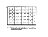 1.0
0.50-
0.50
KSC
0.50
0.60
0.50.
1.0
o.5o
0.50
0.50
t
0.50
0.50
0.50
0.50
0.50
0.50
0.60
0.50
0.50
0.50
0.50
0.50
0.50-
0.50-
0.50.
0.50- -»»
0.50
0.50- »- 0.50-
0.60-»- 0.50-
0.50
0.50
0.50-
Figure 10. Velocity profiles used for underflow scenarios in the WASP4
analysis of the proposed AJ Mine tailings pond. Numbers by arrows
indicate fraction of total flow.
image:
1.0
0.50-
0.50
KSC
0.50
0.60
0.50.
1.0
o.5o
0.50
0.50
t
0.50
0.50
0.50
0.50
0.50
0.50
0.60
0.50
0.50
0.50
0.50
0.50
0.50-
0.50-
0.50.
0.50- -»»
0.50
0.50- »- 0.50-
0.60-»- 0.50-
0.50
0.50
0.50-
Figure 10. Velocity profiles used for underflow scenarios in the WASP4
analysis of the proposed AJ Mine tailings pond. Numbers by arrows
indicate fraction of total flow.
image:
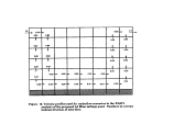 i. Discharge Location:
The applicant has proposed moving the discharge point
periodically so that the tailings will be distributed more or
less uniformly over the bottom of the pond. Furthermore, they
have indicated the discharge point will be no closer to the
proposed dam than 0.5 miles and no farther upstream than 0.5
miles from the Sheep Creek Portal. To simulate the range of
outcomes, the discharge point was located at the most downstream
point indicated by the applicant for certain scenarios and at the
most upstream point for other scenarios. In all cases, discharge
was assumed to be at the bottom of the tailings pond.
7. Simulations
Suspended solids and concentrations of dissolved metals and
metals in suspended solids in the proposed tailings pond and in
the sediments beneath the table were simulated under the
following conditions:
Operation of Mine
1. Initialize the reservoir on January 1 at a depth of
approximately 20 ft (6.0 meters).
2. Begin simulation on January 1 of a fictitious year
assuming inflow from Sheep Creek is constant at a rate
equal to the annual average flow given in the FEIS.
3. Begin discharge of tailings on January 1 at the rate of
22,500 tons/day (236 kg/second) and discharge continuously
for a period sufficiently long for the system to reach a
steady state (one year appears to be adequate).
4. Discharge water from the tailings pond at a rate equal to
the average annual discharge of Sheep Creek (approximately
49 cfs).
Post-Operational Period
1. Cease discharging tailings to the tailings pond on
December 31 of the first fictitious year. From January 1
of the second fictitious year until the end of the
simulation, the hydrology of Sheep Creek is assumed to be
equal to the estimated annual average flow.
2. Discharge water from the tailings pond'at a rate equal to
the average annual discharge of Sheep Creek for a period
of three years.
50
image:
i. Discharge Location:
The applicant has proposed moving the discharge point
periodically so that the tailings will be distributed more or
less uniformly over the bottom of the pond. Furthermore, they
have indicated the discharge point will be no closer to the
proposed dam than 0.5 miles and no farther upstream than 0.5
miles from the Sheep Creek Portal. To simulate the range of
outcomes, the discharge point was located at the most downstream
point indicated by the applicant for certain scenarios and at the
most upstream point for other scenarios. In all cases, discharge
was assumed to be at the bottom of the tailings pond.
7. Simulations
Suspended solids and concentrations of dissolved metals and
metals in suspended solids in the proposed tailings pond and in
the sediments beneath the table were simulated under the
following conditions:
Operation of Mine
1. Initialize the reservoir on January 1 at a depth of
approximately 20 ft (6.0 meters).
2. Begin simulation on January 1 of a fictitious year
assuming inflow from Sheep Creek is constant at a rate
equal to the annual average flow given in the FEIS.
3. Begin discharge of tailings on January 1 at the rate of
22,500 tons/day (236 kg/second) and discharge continuously
for a period sufficiently long for the system to reach a
steady state (one year appears to be adequate).
4. Discharge water from the tailings pond at a rate equal to
the average annual discharge of Sheep Creek (approximately
49 cfs).
Post-Operational Period
1. Cease discharging tailings to the tailings pond on
December 31 of the first fictitious year. From January 1
of the second fictitious year until the end of the
simulation, the hydrology of Sheep Creek is assumed to be
equal to the estimated annual average flow.
2. Discharge water from the tailings pond'at a rate equal to
the average annual discharge of Sheep Creek for a period
of three years.
50
image:
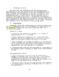 Simulations of TSS, cyanide and various metals were
performed for several different scenarios. Scenarios were
designed to provide a means of assessing the sensitivity of WASP4
simulations to uncertainty in knowledge of important processes.
These processes included:
• vertical mixing due to wind stress, kinetic energy from
advective sources including Sheep Creek and the waste stream
itself and potential energy associated with density
differences
• hydrodynamic regime
• groundwater inflow
• mixing characteristics of sediment pore water
Model parameters which characterize processes for the
various scenarios, and their respective values, are given in
Table 9.
An example of a WASP4 input data set, based on Scenario #1
is given in Appendix C.
8. Results
Simulated steady-state-, values of total solids and solid and
dissolved phases of certain heavy metals associated with the
mining process are given in Tables 10 - 13. During the period
when tailings are being discharged (Tables 10 and 11) , simulated
steady-state levels of total solids and heavy metals in the
effluent from the pond are more sensitive to changes in the
coefficient of vertical eddy diffusivity than in changes to the
hydrodynamic environment. With the exception of total CN, total
concentrations of the chemicals in the discharge are closely
related to the level of TSS in the discharge. Since total CN is
considered only in the dissolved form and is assumed to have an
equilibrium partition coefficient, Kp, equal to zero, it is
dependent only on the amount of dilution provided by the
inflowing freshwater. As is clear from Tables 10 and 11, this
estimated discharge is independent of such- parameters as vertical
mixing rate, settling velocity of solids and hydrodynamic regime
type.
When tailings are discharged at the most upstream point
(Scenarios 1-6), estimated steady-state levels of both total
solids and heavy metals during conditions of high turbulence
(coefficient of .vertical eddy diffusivity = l.OxlO'4 meters2/sec)
are approximately 50% higher than estimates for conditions of low
turbulence (coefficient of vertical eddy diffusivity = 1.0x10'
meters2/sec) . Corresponding variability between estimates when
51
image:
Simulations of TSS, cyanide and various metals were
performed for several different scenarios. Scenarios were
designed to provide a means of assessing the sensitivity of WASP4
simulations to uncertainty in knowledge of important processes.
These processes included:
• vertical mixing due to wind stress, kinetic energy from
advective sources including Sheep Creek and the waste stream
itself and potential energy associated with density
differences
• hydrodynamic regime
• groundwater inflow
• mixing characteristics of sediment pore water
Model parameters which characterize processes for the
various scenarios, and their respective values, are given in
Table 9.
An example of a WASP4 input data set, based on Scenario #1
is given in Appendix C.
8. Results
Simulated steady-state-, values of total solids and solid and
dissolved phases of certain heavy metals associated with the
mining process are given in Tables 10 - 13. During the period
when tailings are being discharged (Tables 10 and 11) , simulated
steady-state levels of total solids and heavy metals in the
effluent from the pond are more sensitive to changes in the
coefficient of vertical eddy diffusivity than in changes to the
hydrodynamic environment. With the exception of total CN, total
concentrations of the chemicals in the discharge are closely
related to the level of TSS in the discharge. Since total CN is
considered only in the dissolved form and is assumed to have an
equilibrium partition coefficient, Kp, equal to zero, it is
dependent only on the amount of dilution provided by the
inflowing freshwater. As is clear from Tables 10 and 11, this
estimated discharge is independent of such- parameters as vertical
mixing rate, settling velocity of solids and hydrodynamic regime
type.
When tailings are discharged at the most upstream point
(Scenarios 1-6), estimated steady-state levels of both total
solids and heavy metals during conditions of high turbulence
(coefficient of .vertical eddy diffusivity = l.OxlO'4 meters2/sec)
are approximately 50% higher than estimates for conditions of low
turbulence (coefficient of vertical eddy diffusivity = 1.0x10'
meters2/sec) . Corresponding variability between estimates when
51
image:
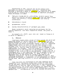 Table 9. Description of scenarios used to assess sensitivity of WASP4 simulations
Scenario Hydrodynamic
Flow Regime
1 Underflow
2 Underfow
3 Uniform Flow
4 Uniform Flow
5 Surface flow
6 Surface Flow
7 Underflow
8 Underfow
9 Uniform Flow
1 0 Uniform Flow
t 1 Surface flow
1 2 Surface Flow
11 T TnifnrfYi f?|/\uf
j uniionu now
1A I Inifnnti Flr\\i/
*f uiiiiuiiii riuw
1C 1 In i if\rm Firtvx/
j LJII 1 lUf III I1VJW
Discharge
Location
Upstream
Upstream
Upstream
Upstream
Upstream
Upstream
Downstream
Downstream
Downstream
Downstream
Downstream
Downstream
Groundwater
Flow
(meters3/sec)
0.0
0.0
0.0
0.0
0.0
0.0
0.0
0.0
0.0
0.0
0.0
0.0
0 0
\J t \f
0 198
\r t \ s \J
0.198
Coefficient of
Vertical
Eddy Diffusivity
(meters^/sec)
l.OOxlO-5
l.OOxlO-4
l.OOxlO-5
l.OOxlO'4
l.OOxlO-5
l.OOxlO'4
1.00x10⁻⁵
l.OOxlO"4
l.OOxlO-5
l.OOxlO"4
l.OOxlO'5
l.OOxIO'4
i nn« i n- 5
i .UUX 1 U
i nrtv i n- 5
1 .UUX 1 U
i nn v i n- 4
1 . UU X 1 U
Coefficient of
Molecular
Diffusion
(meters^/sec)
l.OOxlO'9
l.OOxlO'9
l.OOxlO'9
l.OOxlO-9
l.OOxlO"9
l.OOxlO'9
l.OOxlO--9
l.OOxlO'9
l.OOxlO-9
l.OOxlO'9
l.OOxlO'9
l.OOxlO'9
i on* i n-8
1 • */ 1/ A 1 I/
1 OOxlO"9
• t\J\Jf\ 1 \J
1 .OOxlO'9
Settling Velocity
(meters/sec)
Solids 1 1 Solids 2
l.SOxlO-6 3.50x;10'3
1. SOxlO-6 3.50xlO-3
1.50x10⁻⁶ 3.50x10⁻³
1.50x10⁻⁶ 3.50x10⁻³
1.50x10⁻⁶ 3.50x10⁻³
1.50x10⁻⁶ 3.50x10⁻³
1.50x10⁻⁶ 3.50x10⁻³
1.50x10⁻⁶ 3.50x10⁻³
1.50x10⁻⁶ 3.50x10⁻³
1.50x10⁻⁶ 3.50x10⁻³
1.50x10⁻⁶ 3.50x10⁻³
1.50x10⁻⁶ 3.50x10⁻³
1 sftvin"6 ^ sn*ift"3
I . Jl/ A J i/ J . J U A 1 U
i sn*in"6 i soviO"3
1 . J U A 1 U j , J U A J U
i snTflO'6 i SOxlO'3
I , J\J \ I \f J » J \9 \ l.\J
image:
Table 9. Description of scenarios used to assess sensitivity of WASP4 simulations
Scenario Hydrodynamic
Flow Regime
1 Underflow
2 Underfow
3 Uniform Flow
4 Uniform Flow
5 Surface flow
6 Surface Flow
7 Underflow
8 Underfow
9 Uniform Flow
1 0 Uniform Flow
t 1 Surface flow
1 2 Surface Flow
11 T TnifnrfYi f?|/\uf
j uniionu now
1A I Inifnnti Flr\\i/
*f uiiiiuiiii riuw
1C 1 In i if\rm Firtvx/
j LJII 1 lUf III I1VJW
Discharge
Location
Upstream
Upstream
Upstream
Upstream
Upstream
Upstream
Downstream
Downstream
Downstream
Downstream
Downstream
Downstream
Groundwater
Flow
(meters3/sec)
0.0
0.0
0.0
0.0
0.0
0.0
0.0
0.0
0.0
0.0
0.0
0.0
0 0
\J t \f
0 198
\r t \ s \J
0.198
Coefficient of
Vertical
Eddy Diffusivity
(meters^/sec)
l.OOxlO-5
l.OOxlO-4
l.OOxlO-5
l.OOxlO'4
l.OOxlO-5
l.OOxlO'4
1.00x10⁻⁵
l.OOxlO"4
l.OOxlO-5
l.OOxlO"4
l.OOxlO'5
l.OOxIO'4
i nn« i n- 5
i .UUX 1 U
i nrtv i n- 5
1 .UUX 1 U
i nn v i n- 4
1 . UU X 1 U
Coefficient of
Molecular
Diffusion
(meters^/sec)
l.OOxlO'9
l.OOxlO'9
l.OOxlO'9
l.OOxlO-9
l.OOxlO"9
l.OOxlO'9
l.OOxlO--9
l.OOxlO'9
l.OOxlO-9
l.OOxlO'9
l.OOxlO'9
l.OOxlO'9
i on* i n-8
1 • */ 1/ A 1 I/
1 OOxlO"9
• t\J\Jf\ 1 \J
1 .OOxlO'9
Settling Velocity
(meters/sec)
Solids 1 1 Solids 2
l.SOxlO-6 3.50x;10'3
1. SOxlO-6 3.50xlO-3
1.50x10⁻⁶ 3.50x10⁻³
1.50x10⁻⁶ 3.50x10⁻³
1.50x10⁻⁶ 3.50x10⁻³
1.50x10⁻⁶ 3.50x10⁻³
1.50x10⁻⁶ 3.50x10⁻³
1.50x10⁻⁶ 3.50x10⁻³
1.50x10⁻⁶ 3.50x10⁻³
1.50x10⁻⁶ 3.50x10⁻³
1.50x10⁻⁶ 3.50x10⁻³
1.50x10⁻⁶ 3.50x10⁻³
1 sftvin"6 ^ sn*ift"3
I . Jl/ A J i/ J . J U A 1 U
i sn*in"6 i soviO"3
1 . J U A 1 U j , J U A J U
i snTflO'6 i SOxlO'3
I , J\J \ I \f J » J \9 \ l.\J
image:
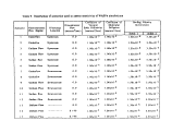 Table 10. Steady-state values of total solids, arsenic, cadmium chromium and copper in the discharge from
the proposed AJ Mine taiings pond during operation of the proposed mine as simulated by WASP4. Parameters
associated with each of the Scenarios are given in Table 9.
Scenario
#
1
2
3
4
5
6
7
8
9
10
1 1
12
Total
Solids
(mg/l)
850
1200
790
1200
760
1200
1200
1700
1 100
1700
940
1800
Arsenic
(UE/1)
Total
9
13
8
1 3
8
1 3
12
17
1 1
1 7
10
1 7
Dissolved
1.5
1.4
1.5
1.4
1.5
1.4
0.8
0.4
0.9
0.3
0.9
0.3
Cadmium
(H /I)
Total
9.9
14.0
9.3
14.1
9.0
14.1
13.9
19.3
12.1
19.0
10.8
19.6
Dissolved
1.3
1.2
1.3
1.2
1.3
1.2
0.7
0.3
0.7
0.3
0.7
0.3
Chromium
(WR/1)
Total
3 1
44
29
44
28
44
44
61
38
6 1
34
62
Dissolved
2.8
2.5
2.9
2.5
2.9
2.6
1.4
0.6
1.5
0.6
1.6
0.5
Copper
(UR/I)
Total
260
360
250
360
240
360
340
470
300
460
270
480
Dissolved
70
73
72
74
7 1
74
43
24
44
25
45
24
image:
Table 10. Steady-state values of total solids, arsenic, cadmium chromium and copper in the discharge from
the proposed AJ Mine taiings pond during operation of the proposed mine as simulated by WASP4. Parameters
associated with each of the Scenarios are given in Table 9.
Scenario
#
1
2
3
4
5
6
7
8
9
10
1 1
12
Total
Solids
(mg/l)
850
1200
790
1200
760
1200
1200
1700
1 100
1700
940
1800
Arsenic
(UE/1)
Total
9
13
8
1 3
8
1 3
12
17
1 1
1 7
10
1 7
Dissolved
1.5
1.4
1.5
1.4
1.5
1.4
0.8
0.4
0.9
0.3
0.9
0.3
Cadmium
(H /I)
Total
9.9
14.0
9.3
14.1
9.0
14.1
13.9
19.3
12.1
19.0
10.8
19.6
Dissolved
1.3
1.2
1.3
1.2
1.3
1.2
0.7
0.3
0.7
0.3
0.7
0.3
Chromium
(WR/1)
Total
3 1
44
29
44
28
44
44
61
38
6 1
34
62
Dissolved
2.8
2.5
2.9
2.5
2.9
2.6
1.4
0.6
1.5
0.6
1.6
0.5
Copper
(UR/I)
Total
260
360
250
360
240
360
340
470
300
460
270
480
Dissolved
70
73
72
74
7 1
74
43
24
44
25
45
24
image:
 Table 11. Steady-state values of mercury, lead, selenium and zinc in the discharge from the proposed AJ
Mine taiings pond during operation of the proposed mine as simulated by WASP4. Parameters associated with each
of the Scenarios are given in Table 9.
Scenario
#
1
2
3
4
5
6
7
8
9
1 0
1 1
1 2
Mercu
(Ug/l)
Total
0.30
0.41
0.29
0.42
0.28
0.42
0.38
0.52
0.35
0.52
0.31
0.53
ry
Dissolved
0.1 1
0.13
0.1 1
0.13
0.1 1
0.13
0.08
0.06
0.08
0.06
0.08
0.06
Lead
(us/1)
Total
170
250
160
250
150
250
250
340
220
360
190
350
Dissolved
3.7
3.2
3.8
3.2
3.7
3.2
1.8
0.6
1.9
0.6
2.1
0.6
Sele
(u
Total
1.1
1.5
1.1
1.5
1.0
1.5
1.4
1.9
1.3
1.9
1.1
1.9
nium
8/1)
Dissolved
0.4
0.5
0.4
0.5
0.4
0.5
0.3
0.2
0.3
0.2
0.3
0.2
Zinc
(US/1)
Total
460
660
430
660
410
660
650
920
570
910
500
940
Dissolved
1 6
13
1 6
1 3
16
1 3
7
2
8
3
9
2
Cyanide
(UK/I)
Dissolved
430
430
430
430
430
430
430
430
430
430
430
430
image:
Table 11. Steady-state values of mercury, lead, selenium and zinc in the discharge from the proposed AJ
Mine taiings pond during operation of the proposed mine as simulated by WASP4. Parameters associated with each
of the Scenarios are given in Table 9.
Scenario
#
1
2
3
4
5
6
7
8
9
1 0
1 1
1 2
Mercu
(Ug/l)
Total
0.30
0.41
0.29
0.42
0.28
0.42
0.38
0.52
0.35
0.52
0.31
0.53
ry
Dissolved
0.1 1
0.13
0.1 1
0.13
0.1 1
0.13
0.08
0.06
0.08
0.06
0.08
0.06
Lead
(us/1)
Total
170
250
160
250
150
250
250
340
220
360
190
350
Dissolved
3.7
3.2
3.8
3.2
3.7
3.2
1.8
0.6
1.9
0.6
2.1
0.6
Sele
(u
Total
1.1
1.5
1.1
1.5
1.0
1.5
1.4
1.9
1.3
1.9
1.1
1.9
nium
8/1)
Dissolved
0.4
0.5
0.4
0.5
0.4
0.5
0.3
0.2
0.3
0.2
0.3
0.2
Zinc
(US/1)
Total
460
660
430
660
410
660
650
920
570
910
500
940
Dissolved
1 6
13
1 6
1 3
16
1 3
7
2
8
3
9
2
Cyanide
(UK/I)
Dissolved
430
430
430
430
430
430
430
430
430
430
430
430
image:
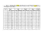 Table 12. Steady-state values of total solids, arsenic, cadmium chromium and copper in the discharge from
the proposed AJ Mine taiings pond after operation of the proposed mine as simulated by WASP4. Parameters
associated with each of the scenarios are given in Table 9.
Scenario
#
1-12
1 3
14
1 5
Arsenic
(WR/D
Total
0.06
0.61
2.0
2.0
Dissolved
0.06
0.61
2.0
2.0
Cadmium
(WR/1)
Total
0.05
0.43
1.4
1.4
Dissolved
0.05
0.43
1.4
1.4
Chromium
(UR/D
Total
0.09
0.84
2.8
2.8
Dissolved
0.09
0.84
2.8
2.8
Copper
(WR/D
Total
5.9
56
190
190
Dissolved
5.9
56
190
190
image:
Table 12. Steady-state values of total solids, arsenic, cadmium chromium and copper in the discharge from
the proposed AJ Mine taiings pond after operation of the proposed mine as simulated by WASP4. Parameters
associated with each of the scenarios are given in Table 9.
Scenario
#
1-12
1 3
14
1 5
Arsenic
(WR/D
Total
0.06
0.61
2.0
2.0
Dissolved
0.06
0.61
2.0
2.0
Cadmium
(WR/1)
Total
0.05
0.43
1.4
1.4
Dissolved
0.05
0.43
1.4
1.4
Chromium
(UR/D
Total
0.09
0.84
2.8
2.8
Dissolved
0.09
0.84
2.8
2.8
Copper
(WR/D
Total
5.9
56
190
190
Dissolved
5.9
56
190
190
image:
 Table 13. Steady-state values of mercury, lead, selenium and zinc in the discharge from the proposed AJ
Mine taiings pond after operation of the proposed mine as simulated by WASP4. Parameters associated with each of
the Scenarios are given in Table 9.
Scenario
#
1-12
13-
14
1 5
Mercury
(ue/1)
Total
0.022
0.215
0.71
0.71
Dissolved
0.022
0.215
0.71
0.71
Lead
(ue/1)
Total
0.084
0.844
2.65
2.65
Dissolved
0.084
0.844
2.65
2.65
Selenum
(ue/1)
Total
0.072
0.686
2.29
2.29
Dissolved
0.072
0.686
2.29
2.29
Zinc
(UR/D
Total
0.387
3.70
1 1.9
1 1.9
Dissolved
0.387
3.70
11.9
11.9
image:
Table 13. Steady-state values of mercury, lead, selenium and zinc in the discharge from the proposed AJ
Mine taiings pond after operation of the proposed mine as simulated by WASP4. Parameters associated with each of
the Scenarios are given in Table 9.
Scenario
#
1-12
13-
14
1 5
Mercury
(ue/1)
Total
0.022
0.215
0.71
0.71
Dissolved
0.022
0.215
0.71
0.71
Lead
(ue/1)
Total
0.084
0.844
2.65
2.65
Dissolved
0.084
0.844
2.65
2.65
Selenum
(ue/1)
Total
0.072
0.686
2.29
2.29
Dissolved
0.072
0.686
2.29
2.29
Zinc
(UR/D
Total
0.387
3.70
1 1.9
1 1.9
Dissolved
0.387
3.70
11.9
11.9
image:
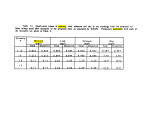 vertical turbulence is held constant is very small for the high
turbulent condition and of the order of 15% for the low level of
turbulence. For discharge at the downstream point (Scenarios 7-
12) , variability of results associated with changes in level of
turbulence is similar to that for upstream discharge. However,
variability of results associated with changes in the
hydrodynamic flow regime is much greater for the downstream
discharge than for the upstream.
Simulated results for the sediment pore water and solids are
not reported. The reason for this is that since the values
reported by Frank (1994) for the effluent solid and dissolved
phases of metals (Table 7) were used to estimate partition
coefficients, simulated results for the sediment concentrations
of metals were the same as the dissolved and solids
concentrations for each of the heavy metals as given in Table 7.
The high metals concentrations in the pore water of the
tailings pond sediment do not have a noticeable impact on
discharge concentrations during the period the mine is in
operation. However, once the mine has stopped discharging
tailings to the pond, the sediment pore water, for the
assumptions made in this application of WASP4, is the primary
source for heavy metals in the overlying water column. For the
base conditions (Scenarios 1-12), the estimated concentrations
of all metals are generally low. Bioturbation of the sediments
(Scenario 13) leads to an increase in discharge concentrations of
metals of an order of magnitude. Inflow of the maximum amount
groundwater (Scenarios 14 and 15) results in a threefold increase
over estimates from the bioturbation conditions.
For the parameters considered in the scenarios (Table 9),
the simulated results for TSS and metals during operation of the
mine were most sensitive to the coefficient of vertical eddy
diffusivity and to the location of the discharge point. As
pointed out previously, the simulated concentration of total CN
was a function of the ratio of freshwater inflow to the rate of
effluent discharge, only. After mining operations cease, the
concentration of metals in the water of the tailings pond is
sensitive.to the rate of bioturbation and to the quantity of
groundwater flow through the sediments.
F^ Effluent Quality Predictions: CE-OUAL-W2 Water Quality Model
1. Conceptual Model
Version 2.04 of CE-QUAL-W2 (Cole and Chapman, 1994) was used
to simulate tailings pond hydrodynamics, tailings pond water
temperature, suspended solids and level of dissolved metals. CE-
Q§AE-W2 has been applied to a wide variety of water bodies which
have small lateral variability and for which density plays an
important role in the hydrodynamics. This includes estuarine
57
image:
vertical turbulence is held constant is very small for the high
turbulent condition and of the order of 15% for the low level of
turbulence. For discharge at the downstream point (Scenarios 7-
12) , variability of results associated with changes in level of
turbulence is similar to that for upstream discharge. However,
variability of results associated with changes in the
hydrodynamic flow regime is much greater for the downstream
discharge than for the upstream.
Simulated results for the sediment pore water and solids are
not reported. The reason for this is that since the values
reported by Frank (1994) for the effluent solid and dissolved
phases of metals (Table 7) were used to estimate partition
coefficients, simulated results for the sediment concentrations
of metals were the same as the dissolved and solids
concentrations for each of the heavy metals as given in Table 7.
The high metals concentrations in the pore water of the
tailings pond sediment do not have a noticeable impact on
discharge concentrations during the period the mine is in
operation. However, once the mine has stopped discharging
tailings to the pond, the sediment pore water, for the
assumptions made in this application of WASP4, is the primary
source for heavy metals in the overlying water column. For the
base conditions (Scenarios 1-12), the estimated concentrations
of all metals are generally low. Bioturbation of the sediments
(Scenario 13) leads to an increase in discharge concentrations of
metals of an order of magnitude. Inflow of the maximum amount
groundwater (Scenarios 14 and 15) results in a threefold increase
over estimates from the bioturbation conditions.
For the parameters considered in the scenarios (Table 9),
the simulated results for TSS and metals during operation of the
mine were most sensitive to the coefficient of vertical eddy
diffusivity and to the location of the discharge point. As
pointed out previously, the simulated concentration of total CN
was a function of the ratio of freshwater inflow to the rate of
effluent discharge, only. After mining operations cease, the
concentration of metals in the water of the tailings pond is
sensitive.to the rate of bioturbation and to the quantity of
groundwater flow through the sediments.
F^ Effluent Quality Predictions: CE-OUAL-W2 Water Quality Model
1. Conceptual Model
Version 2.04 of CE-QUAL-W2 (Cole and Chapman, 1994) was used
to simulate tailings pond hydrodynamics, tailings pond water
temperature, suspended solids and level of dissolved metals. CE-
Q§AE-W2 has been applied to a wide variety of water bodies which
have small lateral variability and for which density plays an
important role in the hydrodynamics. This includes estuarine
57
image:
 systems, as well as freshwater reservoir systems. The model
kinetics in CE-QUAL-W2 generally reflect the current state of
knowledge for simulation of chemical, physical and biological
state variables in estuarine or reservoir systems. The
theoretical basis for the model and the user's manual can be
found in Cole and Buchak (1993).
CE-QUAL-W2 was applied to the AJ Mine tailings pond after a
number of reviewers recommended that a model be used which had
the potential for simulating underflows associated with
differences between inflow density and ambient density structure
of the pond. CE-QUAL-W2 was chosen based on its availability and
widespread usage. CE-QUAL-W2 was not developed to simulate the
kinetics of metals partitioning. Nor was CE-QUAL-W2 developed
to simulate dissolved and solids concentrations in the sediments
accumulating beneath the pond and the interactions between metals
in the sediments and surface water. CE-QUAL-W2 does, however,
simulate suspended solids and conservative constituents in
laterally-averaged surface waters including lakes, reservoirs and
estuaries. The conceptualization of the tailings pond system for
purposes of applying CE-QUAL-W2' was done so as to accommodate
this limitation without making substantive changes to what is a
complex system of software. The conceptual model was designed to
assess effects of density flows, variability in environmental
conditions, but to aggregate geochemical processes in a manner
consistent with the existing capabilities of CE-QUAL-W2. Since
CE-QUAL-W2 was not developed to simulate the interchange of
metals between sediments and the overlying water column, there
was little to be gained by using CE-QUAL-W2 to assess water
quality conditions after mining operations cease. Therefore, CE-
QUAL-W2 was used to simulate conditions only while the mine was
in full operation.
In this application of CE-QUAL-W2, the waters of the
tailings impoundment have been conceptualized as a laterally
well-mixed system which is compartmentalized vertically and
horizontally into finite segments for two different operating
levels of the proposed impoundment. These operating levels
correspond to the proposed Stage I level when the impoundment
first begins discharging and the proposed Stage III level when
the impoundment is at maximum level. These two stages correspond
to nominal surface levels of 765 feet above Mean Sea level and
918 feet above Mean Sea Level, respectively. Each of the
segments in both conceptualization is one meter in thickness.
Segment lengths are variable, but on the order of 200-400 meters,
while the widths of each of the segments were determined from
topographical maps provided by the applicant. Longitudinal
sections of each conceptualization are shown in Figures 11 and
12.
The discharge of the mine tailings is assumed to be
distributed instantaneously over the bottom segment at one of six
58
image:
systems, as well as freshwater reservoir systems. The model
kinetics in CE-QUAL-W2 generally reflect the current state of
knowledge for simulation of chemical, physical and biological
state variables in estuarine or reservoir systems. The
theoretical basis for the model and the user's manual can be
found in Cole and Buchak (1993).
CE-QUAL-W2 was applied to the AJ Mine tailings pond after a
number of reviewers recommended that a model be used which had
the potential for simulating underflows associated with
differences between inflow density and ambient density structure
of the pond. CE-QUAL-W2 was chosen based on its availability and
widespread usage. CE-QUAL-W2 was not developed to simulate the
kinetics of metals partitioning. Nor was CE-QUAL-W2 developed
to simulate dissolved and solids concentrations in the sediments
accumulating beneath the pond and the interactions between metals
in the sediments and surface water. CE-QUAL-W2 does, however,
simulate suspended solids and conservative constituents in
laterally-averaged surface waters including lakes, reservoirs and
estuaries. The conceptualization of the tailings pond system for
purposes of applying CE-QUAL-W2' was done so as to accommodate
this limitation without making substantive changes to what is a
complex system of software. The conceptual model was designed to
assess effects of density flows, variability in environmental
conditions, but to aggregate geochemical processes in a manner
consistent with the existing capabilities of CE-QUAL-W2. Since
CE-QUAL-W2 was not developed to simulate the interchange of
metals between sediments and the overlying water column, there
was little to be gained by using CE-QUAL-W2 to assess water
quality conditions after mining operations cease. Therefore, CE-
QUAL-W2 was used to simulate conditions only while the mine was
in full operation.
In this application of CE-QUAL-W2, the waters of the
tailings impoundment have been conceptualized as a laterally
well-mixed system which is compartmentalized vertically and
horizontally into finite segments for two different operating
levels of the proposed impoundment. These operating levels
correspond to the proposed Stage I level when the impoundment
first begins discharging and the proposed Stage III level when
the impoundment is at maximum level. These two stages correspond
to nominal surface levels of 765 feet above Mean Sea level and
918 feet above Mean Sea Level, respectively. Each of the
segments in both conceptualization is one meter in thickness.
Segment lengths are variable, but on the order of 200-400 meters,
while the widths of each of the segments were determined from
topographical maps provided by the applicant. Longitudinal
sections of each conceptualization are shown in Figures 11 and
12.
The discharge of the mine tailings is assumed to be
distributed instantaneously over the bottom segment at one of six
58
image:
 3.7km
6.1 meters
Figure 11. Two-dimensonal grid used for CE-QUAL-W2 simulations for tailings pond
in Stage I. Nominal surface elevation of the pond is 233.0 meters above sea level.
image:
3.7km
6.1 meters
Figure 11. Two-dimensonal grid used for CE-QUAL-W2 simulations for tailings pond
in Stage I. Nominal surface elevation of the pond is 233.0 meters above sea level.
image:
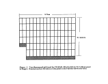 4.6km
6.1 meters
Figure 12. Two-dimensonal grid used for CE-QUAL-W2 simulations for tailings pond
in Stage III. Nominal surface elevation of the pond is 279.5 meters above sea level.
image:
4.6km
6.1 meters
Figure 12. Two-dimensonal grid used for CE-QUAL-W2 simulations for tailings pond
in Stage III. Nominal surface elevation of the pond is 279.5 meters above sea level.
image:
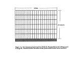 locations in the tailings pond. The six locations were chosen to
represent approximately evenly distributed points spanning the
maximum excursion of the elephant trunk barge as indicated by the
applicant (Bergstrom, 1994). Once the tailings are distributed
in the water column the levels of solids and associated dissolved
and particulate concentrations of metals in the water column are
determined by the following processes:
• Settling rates of a single class of tailings solids
• Longitudinal mixing in the tailings pond due to various
energy sources
• Vertical mixing in the tailings pond due to various
energy sources including wind stress and kinetic energy
• Rates of inflow surface water, groundwater and
effluent from the mining process
• Rates of outflow of recycle water from the tailings
pond
• Rates of discharge from the impoundment
• Potential energy developed in the impoundment due to
solar heating
2. Time and Length Scales
The waters of the proposed tailings pond are conceptualized
as being comprised of a number of vertically and laterally well-
mixed compartments the size of the project, or with overall
length scales corresponding to the size of the tailings pond at
Stage I (765 feet above Mean Sea Level) and Stage III (918 feet
above Mean Sea Level). The CE-QUAL-W2 model formulation will
resolve laterally-averaged concentration differences at scales
of approximately the element size, which is one meter vertically
and 200-400 meters longitudinally. The length scales are best
professional estimates of what is needed to resolve details of
the problem associated with deposition, resuspension and
injection of the waste stream.
There are a number of time scales which may influence model
results. The simulation time period (time step) for the
numerical scheme used is of the order of minutes. The simulation
time period does have an effect on simulation accuracy, but the
fact that this time period is of the order of minutes does not
mean the model is simulating processes in the tailings pond at
this scale. The process time scales in the tailings pond and
sediments which can be resolved by the simulation are determined
by the rate of inflow of the waste stream, Sheep Creek and
groundwater; the amount of storage in the tailings pond; the
61
image:
locations in the tailings pond. The six locations were chosen to
represent approximately evenly distributed points spanning the
maximum excursion of the elephant trunk barge as indicated by the
applicant (Bergstrom, 1994). Once the tailings are distributed
in the water column the levels of solids and associated dissolved
and particulate concentrations of metals in the water column are
determined by the following processes:
• Settling rates of a single class of tailings solids
• Longitudinal mixing in the tailings pond due to various
energy sources
• Vertical mixing in the tailings pond due to various
energy sources including wind stress and kinetic energy
• Rates of inflow surface water, groundwater and
effluent from the mining process
• Rates of outflow of recycle water from the tailings
pond
• Rates of discharge from the impoundment
• Potential energy developed in the impoundment due to
solar heating
2. Time and Length Scales
The waters of the proposed tailings pond are conceptualized
as being comprised of a number of vertically and laterally well-
mixed compartments the size of the project, or with overall
length scales corresponding to the size of the tailings pond at
Stage I (765 feet above Mean Sea Level) and Stage III (918 feet
above Mean Sea Level). The CE-QUAL-W2 model formulation will
resolve laterally-averaged concentration differences at scales
of approximately the element size, which is one meter vertically
and 200-400 meters longitudinally. The length scales are best
professional estimates of what is needed to resolve details of
the problem associated with deposition, resuspension and
injection of the waste stream.
There are a number of time scales which may influence model
results. The simulation time period (time step) for the
numerical scheme used is of the order of minutes. The simulation
time period does have an effect on simulation accuracy, but the
fact that this time period is of the order of minutes does not
mean the model is simulating processes in the tailings pond at
this scale. The process time scales in the tailings pond and
sediments which can be resolved by the simulation are determined
by the rate of inflow of the waste stream, Sheep Creek and
groundwater; the amount of storage in the tailings pond; the
61
image:
 rates of vertical diffusion; the response time of the system to
imposed wind stresses; and the seasonal input of energy from
solar radiation.
3_. Important Assumptions
As in the case of the WASP4 simulations, data from the EIS
and from other relevant sources were used to implement the
conceptual model. These sources provided the basis for defining
important parameters used in the simulations. The fixed
parameter values used in the simulations are given in Table 6.
The implementation of WASP for this problem included the
following assumptions:
• The surface level of the tailings pond is determined by the
water balance and the geometry of the tailings pond. As
described previously, two tailings pond geometry's were
considered; one corresponding to the lowest level of
operation, the other to the maximum level of operation.
• The bottom of the impoundment remains at a constant level,
approximately 20 feet below the water surface.
• The water balance, including effluent flow rates,
groundwater flow rates, outflow rates and recycle flow
rates, was similar to that used by SRK (1994).
• Settling rates of particles are determined from Stokes1 Law
• The tailings slurry comprises only one particle class. The
particle size of this fraction is assumed to be equal to the
minimum particle size reported by Knight and Piesold
(1989) .
• Settling velocities for the particle class can be estimated
from Stokes1 Law using the median diameter for each
fraction, or the lowest reported value, in cases where the
particle size of any fraction was not given in any reports
provided by the applicant.
• Dissolved metals can be treated as conservative constituents
with no leaching or partitioning between solid and
dissolved.
• Dissolved levels of metals in Sheep Creek are constant.
62
image:
rates of vertical diffusion; the response time of the system to
imposed wind stresses; and the seasonal input of energy from
solar radiation.
3_. Important Assumptions
As in the case of the WASP4 simulations, data from the EIS
and from other relevant sources were used to implement the
conceptual model. These sources provided the basis for defining
important parameters used in the simulations. The fixed
parameter values used in the simulations are given in Table 6.
The implementation of WASP for this problem included the
following assumptions:
• The surface level of the tailings pond is determined by the
water balance and the geometry of the tailings pond. As
described previously, two tailings pond geometry's were
considered; one corresponding to the lowest level of
operation, the other to the maximum level of operation.
• The bottom of the impoundment remains at a constant level,
approximately 20 feet below the water surface.
• The water balance, including effluent flow rates,
groundwater flow rates, outflow rates and recycle flow
rates, was similar to that used by SRK (1994).
• Settling rates of particles are determined from Stokes1 Law
• The tailings slurry comprises only one particle class. The
particle size of this fraction is assumed to be equal to the
minimum particle size reported by Knight and Piesold
(1989) .
• Settling velocities for the particle class can be estimated
from Stokes1 Law using the median diameter for each
fraction, or the lowest reported value, in cases where the
particle size of any fraction was not given in any reports
provided by the applicant.
• Dissolved metals can be treated as conservative constituents
with no leaching or partitioning between solid and
dissolved.
• Dissolved levels of metals in Sheep Creek are constant.
62
image:
 4. Parameter Estimation
The density of the tailings, rt, was obtained from results
reported by Knight and Piesold (1989).
The fraction of important metals in the digested slurry, for
both solid and dissolved phases were estimated from various data
sources as described in Section VI.D. These estimates are given
in Table 7.
a. Vertical Mixing
Rates of vertical diffusion in the tailings pond will be
determined by the levels of available turbulent energy. In CE-
QUAL-W2, these levels are estimated using a turbulent closure
scheme based on the Richardson number. Coefficients of vertical
eddy diffusivity are calculated by CE-QUAL-W2 using the simulated
vertical density structure and the simulated vertical shear.
These parameters are, of course, influenced by buoyancy flux from
external sources, heat exchange between the water body and the
atmosphere and wind speed and fetch. The closure scheme includes
a minimum level of vertical mixing such that turbulence
unaccounted for by the Richardson number closure scheme can be
included. Based on discussions with the applicant (Bergstrom,
1993) and results from shallow lakes (Bowie et al, 1985), the
minimum level for the coefficient of vertical eddy diffusivity
for all constituents was chosen to be l.OxlCT5 meters2/second.
The net result is that the CE-QUAL-W2 simulation software will
compute the vertical eddy diffusivity based on the Richardson
number, but will use the computed value only if it exceeds the
minimum value of l.OxlCT5 meters2/second. If the computed value
does not exceed the minimum, the minimum value is used as the
estimate.
b. Initial Mixing of Discharge
The initial mixing characteristics of the discharge were
assumed to be the same for the CE-QUAL-W2 base case simulations
as for the WASP4 simulations described previously. That is 2.5%
of the total loading, as represented by the smallest 2.5th
percentile of particles were assumed to be suspended in the
lowest one meter at the time of initial discharge.
c. Settling
The settling velocity for the base case conditions, (2.5% of
the material initially suspended in the water column in the
segment to which discharge is made) was assumed to be the same as
that described for the WASP4 simulations.
63
image:
4. Parameter Estimation
The density of the tailings, rt, was obtained from results
reported by Knight and Piesold (1989).
The fraction of important metals in the digested slurry, for
both solid and dissolved phases were estimated from various data
sources as described in Section VI.D. These estimates are given
in Table 7.
a. Vertical Mixing
Rates of vertical diffusion in the tailings pond will be
determined by the levels of available turbulent energy. In CE-
QUAL-W2, these levels are estimated using a turbulent closure
scheme based on the Richardson number. Coefficients of vertical
eddy diffusivity are calculated by CE-QUAL-W2 using the simulated
vertical density structure and the simulated vertical shear.
These parameters are, of course, influenced by buoyancy flux from
external sources, heat exchange between the water body and the
atmosphere and wind speed and fetch. The closure scheme includes
a minimum level of vertical mixing such that turbulence
unaccounted for by the Richardson number closure scheme can be
included. Based on discussions with the applicant (Bergstrom,
1993) and results from shallow lakes (Bowie et al, 1985), the
minimum level for the coefficient of vertical eddy diffusivity
for all constituents was chosen to be l.OxlCT5 meters2/second.
The net result is that the CE-QUAL-W2 simulation software will
compute the vertical eddy diffusivity based on the Richardson
number, but will use the computed value only if it exceeds the
minimum value of l.OxlCT5 meters2/second. If the computed value
does not exceed the minimum, the minimum value is used as the
estimate.
b. Initial Mixing of Discharge
The initial mixing characteristics of the discharge were
assumed to be the same for the CE-QUAL-W2 base case simulations
as for the WASP4 simulations described previously. That is 2.5%
of the total loading, as represented by the smallest 2.5th
percentile of particles were assumed to be suspended in the
lowest one meter at the time of initial discharge.
c. Settling
The settling velocity for the base case conditions, (2.5% of
the material initially suspended in the water column in the
segment to which discharge is made) was assumed to be the same as
that described for the WASP4 simulations.
63
image:
 The settling velocity for those scenarios designed to
evaluate the SETTLE results were based on the zone settling
velocity reported by Hartman Associates (1994).
d. Groundwater
Groundwater inflow was assumed to be constant and equal to 7
cfs as reported by SRK (1994).
e. Avalanches
Impacts of avalanches on the impoundment water quality were
not considered, based on the rationale described previously.
f. Discharge Location
The applicant has proposed moving the discharge point
periodically so that the tailings will be distributed more or
less uniformly over the bottom of the pond. Furthermore, they
have indicated the discharge point will move no farther than one-
half mile downstream from the Sheep Creek Adit and no farther
than one-half upstream from the Sheep Creek Adit. To simulate
the range of outcomes, the discharge point was located for a
period of two months during each year at each of the six
locations representative of barge positioning strategies proposed
by the applicant.
g. Effluent Characteristics
Estimates of the variability in effluent characteristics
were based on the discussion in Bergstrom (1994). A lag-one
Markov model was used to describe the daily loading from the
mining operation according to:
-Q(n)
where,
Q(n) = simulated effluent flow rate from the proposed
facility on the nth day of the year,
meters3/second,
64
image:
The settling velocity for those scenarios designed to
evaluate the SETTLE results were based on the zone settling
velocity reported by Hartman Associates (1994).
d. Groundwater
Groundwater inflow was assumed to be constant and equal to 7
cfs as reported by SRK (1994).
e. Avalanches
Impacts of avalanches on the impoundment water quality were
not considered, based on the rationale described previously.
f. Discharge Location
The applicant has proposed moving the discharge point
periodically so that the tailings will be distributed more or
less uniformly over the bottom of the pond. Furthermore, they
have indicated the discharge point will move no farther than one-
half mile downstream from the Sheep Creek Adit and no farther
than one-half upstream from the Sheep Creek Adit. To simulate
the range of outcomes, the discharge point was located for a
period of two months during each year at each of the six
locations representative of barge positioning strategies proposed
by the applicant.
g. Effluent Characteristics
Estimates of the variability in effluent characteristics
were based on the discussion in Bergstrom (1994). A lag-one
Markov model was used to describe the daily loading from the
mining operation according to:
-Q(n)
where,
Q(n) = simulated effluent flow rate from the proposed
facility on the nth day of the year,
meters3/second,
64
image:
 ~Q(n) = average effluent flow rate from the proposed
facility on the nth day of the year,
meters3 / second,
p = correlation coefficient between effluent flow rate
on the nth and n+lth days,
VQ = random component distributed as N(0,l),
a^ = variance of random fluctuations in effluent flow rate
Effluent concentrations of suspended solids and metals in
the dissolved and solid phases of the discharge were kept
constant using the values given in Table 7.
Stream Inflow Characteristics: Inflow temperatures for stream
temperatures in Sheep Creek were generated from the lag-one
Markov model
where,
T(n) = simulated water temperature in Sheep Creek on the nth
day of the year, °C,
= average water temperature in Sheep Creek on the nthday
of the year based on available data, °C,
T° + DT sin(2p(n - nO)/365.)
To = annual average water temperature in Sheep Creek, °C,
DT = one-half the annual variation in water temperature in
water temperature in Sheep Creek, °C,
n0 = the first day in the year when the daily average water
temperature is equal to the annual average water
temperature, °C,
p = correlation coefficient between temperatures on the nth
T day and n+lth day,
v = random component distributed as N(0,l),
YT
65
image:
~Q(n) = average effluent flow rate from the proposed
facility on the nth day of the year,
meters3 / second,
p = correlation coefficient between effluent flow rate
on the nth and n+lth days,
VQ = random component distributed as N(0,l),
a^ = variance of random fluctuations in effluent flow rate
Effluent concentrations of suspended solids and metals in
the dissolved and solid phases of the discharge were kept
constant using the values given in Table 7.
Stream Inflow Characteristics: Inflow temperatures for stream
temperatures in Sheep Creek were generated from the lag-one
Markov model
where,
T(n) = simulated water temperature in Sheep Creek on the nth
day of the year, °C,
= average water temperature in Sheep Creek on the nthday
of the year based on available data, °C,
T° + DT sin(2p(n - nO)/365.)
To = annual average water temperature in Sheep Creek, °C,
DT = one-half the annual variation in water temperature in
water temperature in Sheep Creek, °C,
n0 = the first day in the year when the daily average water
temperature is equal to the annual average water
temperature, °C,
p = correlation coefficient between temperatures on the nth
T day and n+lth day,
v = random component distributed as N(0,l),
YT
65
image:
 <ir = variance of random fluctuations in daily averaged water
temperature in Sheep Creek
Parameter values for both Markov models are in Table 14.
Daily averaged total suspended solids in the waters of both
Sheep Creek and Gold Creek were treated as independent random
variables distributed lognormally with means and variances in
logarithmic space as given in Table 14. Daily averaged values of
all metals in both Sheep Creek and Gold Creek were assumed to be
below detection limits.
5. Simulations
Suspended solids and concentrations of dissolved metals and
metals in suspended solids in the proposed tailings pond were
simulated under the conditions representing natural variability
of weather and inflow hydrology, as well as estimated variability
in the discharge characteristics. The natural variability in the
inflow hydrology was derived from the 30-year record of
streamflow measurements at the USGS gage in Sheep Creek. The
natural variability in weather data was derived from two sources.
Daily averaged values of dry-bulb temperature, relative humidity,
and wind speed for a three-year period were obtained from the
meteorological station maintained by the applicant during the
period 1991-1993. Daily averaged cloud cover data were obtained
from data collected at the Juneau airport during the five years,
1987, 1989-1992.
Based on the recommendations of the panel of experts, as
described previously under the WASP4 simulations, two basic
scenarios were considered (Scenarios Cl and C2 in Table 15) . The
difference between these two scenarios was in the configuration
of the pond, only. Scenario Cl uses the geometry of the pond
when discharge from the pond first begins (Stage I). Scenario C2
uses the geometry corresponding to the pond configuration in the
final year of operation of the mining facility. All other
parameters, including coefficients of eddy diffusivity, settling
rates and percentage of fines suspended initially in the water
column are based on the recommendation of experts. An example
of the input to CE-QUAL-W2, based on Scenario Cl, is given in
Appendix B.
Two additional scenarios, C3 and C4, were added after the
expert panel had convened and after much of both the WASP4 and
CE-QUAL-W2 modeling had been completed. These two scenarios were
added in an effort to incorporate additional, but incomplete data
provided by the applicant on settling rates. The data are from
results obtained by Hartman Associates (1994). Krone (1994)
stated that these data were not adequate to estimate settling
velocities for the solids. However, in the interests of
66
image:
<ir = variance of random fluctuations in daily averaged water
temperature in Sheep Creek
Parameter values for both Markov models are in Table 14.
Daily averaged total suspended solids in the waters of both
Sheep Creek and Gold Creek were treated as independent random
variables distributed lognormally with means and variances in
logarithmic space as given in Table 14. Daily averaged values of
all metals in both Sheep Creek and Gold Creek were assumed to be
below detection limits.
5. Simulations
Suspended solids and concentrations of dissolved metals and
metals in suspended solids in the proposed tailings pond were
simulated under the conditions representing natural variability
of weather and inflow hydrology, as well as estimated variability
in the discharge characteristics. The natural variability in the
inflow hydrology was derived from the 30-year record of
streamflow measurements at the USGS gage in Sheep Creek. The
natural variability in weather data was derived from two sources.
Daily averaged values of dry-bulb temperature, relative humidity,
and wind speed for a three-year period were obtained from the
meteorological station maintained by the applicant during the
period 1991-1993. Daily averaged cloud cover data were obtained
from data collected at the Juneau airport during the five years,
1987, 1989-1992.
Based on the recommendations of the panel of experts, as
described previously under the WASP4 simulations, two basic
scenarios were considered (Scenarios Cl and C2 in Table 15) . The
difference between these two scenarios was in the configuration
of the pond, only. Scenario Cl uses the geometry of the pond
when discharge from the pond first begins (Stage I). Scenario C2
uses the geometry corresponding to the pond configuration in the
final year of operation of the mining facility. All other
parameters, including coefficients of eddy diffusivity, settling
rates and percentage of fines suspended initially in the water
column are based on the recommendation of experts. An example
of the input to CE-QUAL-W2, based on Scenario Cl, is given in
Appendix B.
Two additional scenarios, C3 and C4, were added after the
expert panel had convened and after much of both the WASP4 and
CE-QUAL-W2 modeling had been completed. These two scenarios were
added in an effort to incorporate additional, but incomplete data
provided by the applicant on settling rates. The data are from
results obtained by Hartman Associates (1994). Krone (1994)
stated that these data were not adequate to estimate settling
velocities for the solids. However, in the interests of
66
image:
 Table 14. Important parameters and their values as used in the lag-one
Markov models to simulate temperature and suspended solids in the
tailings effluent and in Sheep Creek and Gold Creek.
Parameter Description Value
Effluent flow 0.6
correlation coefficient
Standard deviation of 0.4 cfs
effluent flow
pT . Correlation coefficient 0.6
of water temperature
OT Standard deviation of 1.0 °C
water temperature
no Temperature lag 135 days
Variation in water 2.4 °C
temperature
TO Annual average Sheep 4.9 °C
Creek temperature
log mean of TSS in 0.43558
Sheep Creek
log standard deviation 1.48
of TSS in Sheep Creek
log mean of TSS in L07304
Gold Creek
og standard deviation of 1.04042
TSS in Gold Creek
image:
Table 14. Important parameters and their values as used in the lag-one
Markov models to simulate temperature and suspended solids in the
tailings effluent and in Sheep Creek and Gold Creek.
Parameter Description Value
Effluent flow 0.6
correlation coefficient
Standard deviation of 0.4 cfs
effluent flow
pT . Correlation coefficient 0.6
of water temperature
OT Standard deviation of 1.0 °C
water temperature
no Temperature lag 135 days
Variation in water 2.4 °C
temperature
TO Annual average Sheep 4.9 °C
Creek temperature
log mean of TSS in 0.43558
Sheep Creek
log standard deviation 1.48
of TSS in Sheep Creek
log mean of TSS in L07304
Gold Creek
og standard deviation of 1.04042
TSS in Gold Creek
image:
 evaluating all "available information, an effort was made to
incorporate this data into modeling scenarios. Analysis of the
referenced measurements by Hartman Associates (1994), using the
US Army Corps of Engineers (USAGE, 1987) SETTLE model, gave
results of zone settling rates for the effluent in a static test
column. According to the USAGE (1987), zone settling is used to
determine the area of the settling pond and not for estimating
the concentration of solids in the discharge from the pond.
Since this was the only new analysis available at the time CE-
QUAL-W2 was applied to the problem, two scenarios were developed
based on zone settling rates. This was done by assuming that
100% of the material was injected into the pond at the bottom and
that it settled at the rate of zone settling computed by Hartman
Associates (1994). This rate was 1.77 meters/day or 2.0xlO"5
meters/second. As shown in Table 15, all parameters and
conditions other than the settling rate and the percent of
material suspended in the water column, is the same as for
Scenarios Cl and C2.
For all four scenarios, a 30-year simulation was performed
in which the inflow hydrology w'as taken from the existing 30-year
record of flows at the USGS gaging station. Outflow from the
impoundment was based on the rule curve provided by SRK (1994).
For each year of streamflow, a year of cloud cover was chosen at
random from the five years of data collected at the Juneau
airport and a year of dry-bulb temperature, relative humidity,
and wind speed was chosen at random from the three-year record
obtained by the applicant at the meteorological station in Sheep
Creek valley.
Using the environmental inputs described above, CE-QUAL-W2
was used to simulate laterally-averaged vertical and longitudinal
velocities, water temperature, suspended solids and a
hypothetical conservative substance. The hypothetical
conservative substance was used to represent concentrations of
dissolved metals. The concentration of the hypothetical
conservative substance in the tailings discharge was assumed to
be 100 units. The concentration of dissolved metals in the
outflow from the impoundment, C^t^, for those metals listed in
Table 7, was estimated from
f,OUC
,out ,-, e£tlueae v ^eoaaervaciva -, eff1 uenc *•cougarvativo
= X-
^r t*J.±J.U9JI*~ 100
<-conservative
Concentrations of metals in the solid phase were calculated
using the ratio of metals to solids given in Table 7.
The resulting concentrations of metals in solid and
dissolved phases, obtained from CE-QUAL-W2 for the 30-year
simulations, were combined with a similar 30-year hydrologic
68
image:
evaluating all "available information, an effort was made to
incorporate this data into modeling scenarios. Analysis of the
referenced measurements by Hartman Associates (1994), using the
US Army Corps of Engineers (USAGE, 1987) SETTLE model, gave
results of zone settling rates for the effluent in a static test
column. According to the USAGE (1987), zone settling is used to
determine the area of the settling pond and not for estimating
the concentration of solids in the discharge from the pond.
Since this was the only new analysis available at the time CE-
QUAL-W2 was applied to the problem, two scenarios were developed
based on zone settling rates. This was done by assuming that
100% of the material was injected into the pond at the bottom and
that it settled at the rate of zone settling computed by Hartman
Associates (1994). This rate was 1.77 meters/day or 2.0xlO"5
meters/second. As shown in Table 15, all parameters and
conditions other than the settling rate and the percent of
material suspended in the water column, is the same as for
Scenarios Cl and C2.
For all four scenarios, a 30-year simulation was performed
in which the inflow hydrology w'as taken from the existing 30-year
record of flows at the USGS gaging station. Outflow from the
impoundment was based on the rule curve provided by SRK (1994).
For each year of streamflow, a year of cloud cover was chosen at
random from the five years of data collected at the Juneau
airport and a year of dry-bulb temperature, relative humidity,
and wind speed was chosen at random from the three-year record
obtained by the applicant at the meteorological station in Sheep
Creek valley.
Using the environmental inputs described above, CE-QUAL-W2
was used to simulate laterally-averaged vertical and longitudinal
velocities, water temperature, suspended solids and a
hypothetical conservative substance. The hypothetical
conservative substance was used to represent concentrations of
dissolved metals. The concentration of the hypothetical
conservative substance in the tailings discharge was assumed to
be 100 units. The concentration of dissolved metals in the
outflow from the impoundment, C^t^, for those metals listed in
Table 7, was estimated from
f,OUC
,out ,-, e£tlueae v ^eoaaervaciva -, eff1 uenc *•cougarvativo
= X-
^r t*J.±J.U9JI*~ 100
<-conservative
Concentrations of metals in the solid phase were calculated
using the ratio of metals to solids given in Table 7.
The resulting concentrations of metals in solid and
dissolved phases, obtained from CE-QUAL-W2 for the 30-year
simulations, were combined with a similar 30-year hydrologic
68
image:
 Table 15. Description of scenarios used in CE-QUAL-W2 simulations
Scenario
C-l
C-2
C-3
C--4
Pond
Stage
Stage I
Stage III
Stage I
Stage III
% Fines
Suspended in
Water Column
2.5
2.5
100
100
Groundwater
Flow
(meters^/sec)
0.198
0.198
0.198
0.198
Minimum
Vertical
Eddy Diffusivity
(meters^/sec)
l.OOxlO'5
l.OOxlO'5
l.OOxlO-5
1.00x10⁻⁵
Settling Velocity
(meters/sec)
Solids 1
l.SOxlO-6
1.50xlO-6
1.50x10⁻⁶
1.50x10⁻⁶
image:
Table 15. Description of scenarios used in CE-QUAL-W2 simulations
Scenario
C-l
C-2
C-3
C--4
Pond
Stage
Stage I
Stage III
Stage I
Stage III
% Fines
Suspended in
Water Column
2.5
2.5
100
100
Groundwater
Flow
(meters^/sec)
0.198
0.198
0.198
0.198
Minimum
Vertical
Eddy Diffusivity
(meters^/sec)
l.OOxlO'5
l.OOxlO'5
l.OOxlO-5
1.00x10⁻⁵
Settling Velocity
(meters/sec)
Solids 1
l.SOxlO-6
1.50xlO-6
1.50x10⁻⁶
1.50x10⁻⁶
image:
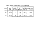 record from Gold Creek. The fraction of flow captured from Gold
Creek and diverted through the diffuser with Sheep Creek
impoundment outflow was calculated using the capture ratios
provided by SRK (1994). The metals concentrations estimated from
the flow-weighted values of simulated Sheep Creek impoundment
metals and Gold Creek water diverted to the discharge pipe
diffuser in Gastineau Channel were used to develop cumulative
distribution functions (CDF's) for each scenario.
This analysis resulted in daily estimates of total suspended
solids and total metals in the discharge for a 30-year period.
Since the analysis was developed from a conceptual model which
included the natural variability in streamflow and meteorology
and projected variability in the effluent characteristics, it was
assumed that this 30-year sample could be used to describe the
statistical properties of the simulated effluent concentrations.
This was done by ordering the 30-year record of simulated results
from lowest to highest and then computing the plotting position
of each simulated concentration using the method proposed by Blom
(1958). That is,
PP = (i-0.375)/(N+0.25)
where
PP = the plotting position
i = the rank or order of the simulated result
N= the total number of simulated results
For example, if a simulated concentration of 100 was
determined to be ranked 365th, that is there were 364 results
lower than 100, its plotting position in sample of 30x365 or
10950 simulated results would be:
PP=(365-0.375)/(10950.25)=0.033
Plotting positions are calculated for each of the 10950
simulated results and used to develop the empirical cumulative
distribution function (CDF) for TSS and total metals in the
effluent. The CDF gives the estimated probability that the
effluent concentration of TSS or total metals will be no greater
than some certain value. For the example given above, the
estimated probability that the concentration would never be any
greater than 100 would be 0.033.
6.. Results
Simulated cumulative distribution functions (CDF's) for the
scenarios, Cl and C2, which were based on the experts
recommendations are shown in Figures 13-22. Figures 23 and 24
are the CDF's for TSS and total CN from the scenarios, C3 and C4,
derived from the limited data provided by Hartman Associates
70
image:
record from Gold Creek. The fraction of flow captured from Gold
Creek and diverted through the diffuser with Sheep Creek
impoundment outflow was calculated using the capture ratios
provided by SRK (1994). The metals concentrations estimated from
the flow-weighted values of simulated Sheep Creek impoundment
metals and Gold Creek water diverted to the discharge pipe
diffuser in Gastineau Channel were used to develop cumulative
distribution functions (CDF's) for each scenario.
This analysis resulted in daily estimates of total suspended
solids and total metals in the discharge for a 30-year period.
Since the analysis was developed from a conceptual model which
included the natural variability in streamflow and meteorology
and projected variability in the effluent characteristics, it was
assumed that this 30-year sample could be used to describe the
statistical properties of the simulated effluent concentrations.
This was done by ordering the 30-year record of simulated results
from lowest to highest and then computing the plotting position
of each simulated concentration using the method proposed by Blom
(1958). That is,
PP = (i-0.375)/(N+0.25)
where
PP = the plotting position
i = the rank or order of the simulated result
N= the total number of simulated results
For example, if a simulated concentration of 100 was
determined to be ranked 365th, that is there were 364 results
lower than 100, its plotting position in sample of 30x365 or
10950 simulated results would be:
PP=(365-0.375)/(10950.25)=0.033
Plotting positions are calculated for each of the 10950
simulated results and used to develop the empirical cumulative
distribution function (CDF) for TSS and total metals in the
effluent. The CDF gives the estimated probability that the
effluent concentration of TSS or total metals will be no greater
than some certain value. For the example given above, the
estimated probability that the concentration would never be any
greater than 100 would be 0.033.
6.. Results
Simulated cumulative distribution functions (CDF's) for the
scenarios, Cl and C2, which were based on the experts
recommendations are shown in Figures 13-22. Figures 23 and 24
are the CDF's for TSS and total CN from the scenarios, C3 and C4,
derived from the limited data provided by Hartman Associates
70
image:
 (1994). For scenarios Cl and C2, the results, though stated
somewhat differently, are similar to those provided by the
steady-state WASP4 simulations. This implies that the processes
controlling the quality of the effluent in these scenarios are
percent fines suspended.in the water column, settling rate of the
solids, turbulent mixing rates within the pond and the residence
time of the pond.
With respect to scenarios C3 and C4 derived from the limited
column settling tests, TSS levels are two orders of magnitude
less than the TSS levels simulated in scenarios Cl and C2.
Corresponding metals concentrations were not computed for
scenarios C3 and C4. Since the total metals concentrations are
highly dependent on the concentration of solids, the estimated
CDF's for scenarios C3 and C4 will be less in approximately the
same proportion as the CDF's for TSS.
As mentioned earlier in the discussion of the WASP4 results,
the concentration of total CN does not depend on the level of
solids. For this reason, the estimated CDF's for total CN are
similar for all four simulation's using CE-QUAL-W2 and are of the
same order as the results predicted by WASP4.
G.. Discussion of the WASP4 and CE-OUAL-W2 Results
Simulations of water quality in the proposed AJ Mine
tailings pond were obtained, using two different mathematical
models, WASP4 (Ambrose et al, 1991) and CE-QUAL-W2 (Cole and
Buchak, 1993). While these are complex and sophisticated models
based on principles of conservation of matter and energy, model
results are highly dependent on estimates of those parameters
which characterize major processes of the system being modeled,
such as the proportion of tailings that would become suspended
and' the probability that these particles would settle out. In
the case of the proposed AJ Mine tailings pond, data to estimate
these parameters for the specific site were incomplete or not
available. It was, therefore, necessary to obtain parameter
estimates from recognized experts, from the scientific literature
or from environments for which there was some basis for
extrapolation. The resulting estimates of expected discharge
concentrations should be considered in light of what they are,
which is predictions of water quality. .
Due to the lack of existing prototypes, evaluation of the
uncertainty in the results must be based on knowledge of the
uncertainty in those parameters and those processes which are
believed to have greatest influence on the predictions. In the
simulations described in this report, certain parameters such as
settling velocity, percent solids suspended in the water column
and coefficients of eddy diffusivity were fixed or kept within a
range that did not include the known variability. Instead, they
71
image:
(1994). For scenarios Cl and C2, the results, though stated
somewhat differently, are similar to those provided by the
steady-state WASP4 simulations. This implies that the processes
controlling the quality of the effluent in these scenarios are
percent fines suspended.in the water column, settling rate of the
solids, turbulent mixing rates within the pond and the residence
time of the pond.
With respect to scenarios C3 and C4 derived from the limited
column settling tests, TSS levels are two orders of magnitude
less than the TSS levels simulated in scenarios Cl and C2.
Corresponding metals concentrations were not computed for
scenarios C3 and C4. Since the total metals concentrations are
highly dependent on the concentration of solids, the estimated
CDF's for scenarios C3 and C4 will be less in approximately the
same proportion as the CDF's for TSS.
As mentioned earlier in the discussion of the WASP4 results,
the concentration of total CN does not depend on the level of
solids. For this reason, the estimated CDF's for total CN are
similar for all four simulation's using CE-QUAL-W2 and are of the
same order as the results predicted by WASP4.
G.. Discussion of the WASP4 and CE-OUAL-W2 Results
Simulations of water quality in the proposed AJ Mine
tailings pond were obtained, using two different mathematical
models, WASP4 (Ambrose et al, 1991) and CE-QUAL-W2 (Cole and
Buchak, 1993). While these are complex and sophisticated models
based on principles of conservation of matter and energy, model
results are highly dependent on estimates of those parameters
which characterize major processes of the system being modeled,
such as the proportion of tailings that would become suspended
and' the probability that these particles would settle out. In
the case of the proposed AJ Mine tailings pond, data to estimate
these parameters for the specific site were incomplete or not
available. It was, therefore, necessary to obtain parameter
estimates from recognized experts, from the scientific literature
or from environments for which there was some basis for
extrapolation. The resulting estimates of expected discharge
concentrations should be considered in light of what they are,
which is predictions of water quality. .
Due to the lack of existing prototypes, evaluation of the
uncertainty in the results must be based on knowledge of the
uncertainty in those parameters and those processes which are
believed to have greatest influence on the predictions. In the
simulations described in this report, certain parameters such as
settling velocity, percent solids suspended in the water column
and coefficients of eddy diffusivity were fixed or kept within a
range that did not include the known variability. Instead, they
71
image:
 Figure 13. Estimated CDF's for Total Suspended Solids in the proposed
AJ tailings pond discharge for pond Stage I and Stage DI
1.0
0.9 -
0.8 -
0.7 -
H
V
* 0.6 H
0.5-
J 0.4
2
P-
£ 0.3 H
cs
| 0.2 -
U
o.i -i
o.o
Stage I
Stage DDL
400 800 1200
Total Suspended Solids - mg/I
1600
2000
image:
Figure 13. Estimated CDF's for Total Suspended Solids in the proposed
AJ tailings pond discharge for pond Stage I and Stage DI
1.0
0.9 -
0.8 -
0.7 -
H
V
* 0.6 H
0.5-
J 0.4
2
P-
£ 0.3 H
cs
| 0.2 -
U
o.i -i
o.o
Stage I
Stage DDL
400 800 1200
Total Suspended Solids - mg/I
1600
2000
image:
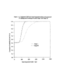 Figure 14. Estimated CDF's for Total As in the proposed AJ tailings
pond discharge for pond Stage I and Stage m
1.0
2
e.
0.9 -
0.8 -
0.7 -
0.6 -
0.5 -
g 0.4 H
JS
2
2 0.3 H
3
S 0.2 -
U
o.i H
o.o
0.000
Stage I
Stage ffl
0.005 0.010
Total As - mg/1
0.015
0.020
image:
Figure 14. Estimated CDF's for Total As in the proposed AJ tailings
pond discharge for pond Stage I and Stage m
1.0
2
e.
0.9 -
0.8 -
0.7 -
0.6 -
0.5 -
g 0.4 H
JS
2
2 0.3 H
3
S 0.2 -
U
o.i H
o.o
0.000
Stage I
Stage ffl
0.005 0.010
Total As - mg/1
0.015
0.020
image:
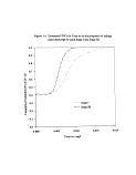 Figure 15. Estimated CDFs for Total Cd in the proposed AJ tailings
pond discharge for pond Stage I and Stage IK
X
£>
2
|
S
1
4>
••*
*3
S
s
i.u -
0.9 -
0.8 -
0.7 -
0.6 -
0.5 -
0.4 -
0 .3 -
0.2-^
0.1 -
0.0 -
/* *
•
»
f
/•
*
*
*
/«
0
*
/ /
/
/ /
/ ..'•'
Stagel
Stage m
. _, , | -
0.000
0.005 0.010
Total Cd - mg/1
0.015
0.020
image:
Figure 15. Estimated CDFs for Total Cd in the proposed AJ tailings
pond discharge for pond Stage I and Stage IK
X
£>
2
|
S
1
4>
••*
*3
S
s
i.u -
0.9 -
0.8 -
0.7 -
0.6 -
0.5 -
0.4 -
0 .3 -
0.2-^
0.1 -
0.0 -
/* *
•
»
f
/•
*
*
*
/«
0
*
/ /
/
/ /
/ ..'•'
Stagel
Stage m
. _, , | -
0.000
0.005 0.010
Total Cd - mg/1
0.015
0.020
image:
 Figure 16. Estimated CDF's for Total Cr in the proposed AJ tailings
pond discharge for pond Stage I and Stage IH
1.0
0.9 -
0.8 -
0.7 -
v
* 0.6 -
0.5 -
2
| 0.4
o
a*
$ 03 H
0.2 -
0.1 -
0.0
0.00
Stage I
StageIH
0.01 0.02 0.03
Total Cr - mg/1
0.04
0.05
image:
Figure 16. Estimated CDF's for Total Cr in the proposed AJ tailings
pond discharge for pond Stage I and Stage IH
1.0
0.9 -
0.8 -
0.7 -
v
* 0.6 -
0.5 -
2
| 0.4
o
a*
$ 03 H
0.2 -
0.1 -
0.0
0.00
Stage I
StageIH
0.01 0.02 0.03
Total Cr - mg/1
0.04
0.05
image:
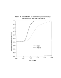 Figure 17. Estimated CDF's for Total Cu in the proposed AJ tailings
pond discharge for pond Stage I and Stage HI
i.u -
0.9 -
0.8 -
0.7 -
V
X 0.6-
JD
s
* 0.5 -
•2 n*
g 0.4 -1
2
&.
V Q^ _
£
| 0.2 -
w
0.1 -
.0 -
0
/"'---""""
/ /•'
/ ..-•'
/ /
//
/••'
• • • • -***
Stage I
Stage in
— 1 1 I
.0 0.2 0.4 0.6 0
.8
Total Cu - mg/1
image:
Figure 17. Estimated CDF's for Total Cu in the proposed AJ tailings
pond discharge for pond Stage I and Stage HI
i.u -
0.9 -
0.8 -
0.7 -
V
X 0.6-
JD
s
* 0.5 -
•2 n*
g 0.4 -1
2
&.
V Q^ _
£
| 0.2 -
w
0.1 -
.0 -
0
/"'---""""
/ /•'
/ ..-•'
/ /
//
/••'
• • • • -***
Stage I
Stage in
— 1 1 I
.0 0.2 0.4 0.6 0
.8
Total Cu - mg/1
image:
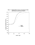 Figure 18. Estimated CDF's for Total Hg in the proposed AJ tailings
pond discharge for pond Stage I and Stage in
1.0
0.9 -
0.8 -
0.7 -
9
*, 0.6 H
2
fe- 0.5 H
| 0.4
2
o-
2 03 H
E 0.2 -
0.1 -
).0
0.0000
1
/I
Stage I
Stage m
1 \
0.0005 0.0010
Total Hg - mg/1
0.0015
0.0020
image:
Figure 18. Estimated CDF's for Total Hg in the proposed AJ tailings
pond discharge for pond Stage I and Stage in
1.0
0.9 -
0.8 -
0.7 -
9
*, 0.6 H
2
fe- 0.5 H
| 0.4
2
o-
2 03 H
E 0.2 -
0.1 -
).0
0.0000
1
/I
Stage I
Stage m
1 \
0.0005 0.0010
Total Hg - mg/1
0.0015
0.0020
image:
 Figure 19. Estimated CDFs for Total Pb in the proposed AJ tailings
pond discharge for pond Stage I and Stage m
1.0
0.9 -
0.8 -
0.7 -
v
* 0.6 H
.0
2
& 0.5 H
"8 0.4
£t
I
I 03 -
S 0 2 -
u
0.1 H
0.0
0.00
x'
/
Stage I
Stage ffl
0.05 0.10 0.15
Total Pb - mg/1
0.20
0.25
image:
Figure 19. Estimated CDFs for Total Pb in the proposed AJ tailings
pond discharge for pond Stage I and Stage m
1.0
0.9 -
0.8 -
0.7 -
v
* 0.6 H
.0
2
& 0.5 H
"8 0.4
£t
I
I 03 -
S 0 2 -
u
0.1 H
0.0
0.00
x'
/
Stage I
Stage ffl
0.05 0.10 0.15
Total Pb - mg/1
0.20
0.25
image:
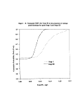 Figure 20. Estimated CDF's for Total Se in the proposed AJ tailings
pond discharge for pond Stage I and Stage EQ
1.0
0.9 -
0.8 -
0.7 -
v
* 0.6 -
0.5 -
2
| 0.4
2
Cu
.> °3 "i
J£
E 0.2 -
0.1 H
0.0
y
0.000
Stage I
Stage in
0.002 0.004
Total Se - mg/I
0.006
0.008
image:
Figure 20. Estimated CDF's for Total Se in the proposed AJ tailings
pond discharge for pond Stage I and Stage EQ
1.0
0.9 -
0.8 -
0.7 -
v
* 0.6 -
0.5 -
2
| 0.4
2
Cu
.> °3 "i
J£
E 0.2 -
0.1 H
0.0
y
0.000
Stage I
Stage in
0.002 0.004
Total Se - mg/I
0.006
0.008
image:
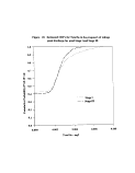 Figure 21. Estimated CDF's for Total Zn in the proposed AJ tailings
pond discharge for pond Stage I and Stage HI
25
V
X,
1
|
3
08
e
£
"a
|
3
i.u -
0.9 -
0.8 -
0.7 -
0.6 -
0.5 -
0.4 -
03 -
«-
0.1 -
.0 -
_ »
f * "
I »
/»
•
* *
I •
/ /
'
/.../
— '
Stage I
Stage m
, -j —i | 1
0.0
0.2 0.4 0.6
Total Zn • mg/l
0.8
1.0
image:
Figure 21. Estimated CDF's for Total Zn in the proposed AJ tailings
pond discharge for pond Stage I and Stage HI
25
V
X,
1
|
3
08
e
£
"a
|
3
i.u -
0.9 -
0.8 -
0.7 -
0.6 -
0.5 -
0.4 -
03 -
«-
0.1 -
.0 -
_ »
f * "
I »
/»
•
* *
I •
/ /
'
/.../
— '
Stage I
Stage m
, -j —i | 1
0.0
0.2 0.4 0.6
Total Zn • mg/l
0.8
1.0
image:
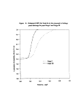 Figure 22. Estimated CDF's for Total CN in the proposed AJ tailings
pond discharge for pond Stage I and Stage HI
1.0
0.9 -
0.8 -
0.7 -
M
* 0.6 H
2
&> 0.5 H
£>
0.4
2
Q*
.>
••*
2
0.1 -
0.0
,7
//
//
//
••• Stage I
— Stage
0.0
-~l I
0.2 0.4
Total CN - mg/1
0.6
0.8
image:
Figure 22. Estimated CDF's for Total CN in the proposed AJ tailings
pond discharge for pond Stage I and Stage HI
1.0
0.9 -
0.8 -
0.7 -
M
* 0.6 H
2
&> 0.5 H
£>
0.4
2
Q*
.>
••*
2
0.1 -
0.0
,7
//
//
//
••• Stage I
— Stage
0.0
-~l I
0.2 0.4
Total CN - mg/1
0.6
0.8
image:
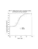 Figure 23. Estimated CDF's for Total Suspended Solids in the proposed AJ
tailings pond discharge for pond Stage I and Stage IIL Settling rates are
derived from zone settling results reported by Hartman & Associates (1994)
1.0
0.9 -
0.8 -
0.7 -
* 0.6 -
2
£• 0.5
£
| 0.4 H
2
CU
| 03 -
2
3
| 0.2 -
o
0.1 -
0.0
Stage I
Stage
40 80 120
Total Suspended Solids - mg/1
160
200
image:
Figure 23. Estimated CDF's for Total Suspended Solids in the proposed AJ
tailings pond discharge for pond Stage I and Stage IIL Settling rates are
derived from zone settling results reported by Hartman & Associates (1994)
1.0
0.9 -
0.8 -
0.7 -
* 0.6 -
2
£• 0.5
£
| 0.4 H
2
CU
| 03 -
2
3
| 0.2 -
o
0.1 -
0.0
Stage I
Stage
40 80 120
Total Suspended Solids - mg/1
160
200
image:
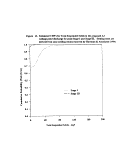 2
a.
Figure 24. Estimated CDF's for Total CN in the proposed AJ tailings
pond discharge for pond Stage I and Stage IEL Settling rates for solids are
derived from zone settling results reported by Hartman & Associates (1994)
1.0
0.9 -
0.8 -
0.7 -
*. 0.6 -
0.5 -
| 0-4
e
E 0.2
0.1 -
0.0
//
.•• /
II
•' /
0.0
0.2 0.4
Total CN - mg/1
0.6
0.8
image:
2
a.
Figure 24. Estimated CDF's for Total CN in the proposed AJ tailings
pond discharge for pond Stage I and Stage IEL Settling rates for solids are
derived from zone settling results reported by Hartman & Associates (1994)
1.0
0.9 -
0.8 -
0.7 -
*. 0.6 -
0.5 -
| 0-4
e
E 0.2
0.1 -
0.0
//
.•• /
II
•' /
0.0
0.2 0.4
Total CN - mg/1
0.6
0.8
image:
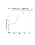 were limited to the best available estimates from experts or from
other studies. However, the results of earlier model studies by
Yearsley (1992, 1993) and Woodward^Clyde Consultants (1993a) show
that the results are quite sensitive to changes in these
parameters. Use of different parameter values.could lead to
outcomes considerably different from those described in this
report. It is interesting to note, that in this case, the
results were not particularly sensitive to the use of a
particular model as was originally expected.
While the work described here, as well as that done
previously (Yearsley, 1992; Yearsley; 1993; Woodward-Clyde
Consultants, 1993a) represents a thorough sensitivity analysis of
certain major processes including settling rates of solids,
percent solids suspended in the water column, turbulent mixing
and hydrologic variability, there are certain other processes to
which limited attention has been given. These include deposition
and resuspension of solids, geochemistry of the pond-effluent
mixture, partitioning characteristics of the discharged metals
between solid and dissolved phases, hydrodynamics of the
subaqueous discharge, and effects of groundwater flow through the
sediments.
The deposition and resuspension issue was discussed briefly
in Yearsley (1993) and Woodward-Clyde Consultants (1993a), but
only in terms of limited information provided by Ambrose et al
(1991). The panel of experts provided some discussion, but the
discussion was not quantitative in terms of environmental
conditions characteristic of this site. Deposition and
resuspension are likely to be affected by the energy dissipated
by the discharge itself, by the extremely high Taku winds which
occur in this valley, and by slumping of the sediments as waste
piles build up on the bottom and become unstable. The slumping
of sediments could be an important factor in resuspending
sediments near the downstream end of the proposed pond where
nominal bottom depths are 20 feet and drop to 45 to 60 feet
within half a mile of the proposed dam (Andrews, 1994) .
The geochemistry of the effluent-pond mixture does not
appear to be an important factor while the mine is in operation,
since the results from the geochemically-based WASP4 simulations
are not greatly different from the dilution-based results based
on the CE-QUAL-W2 results. However, it does appear to be
important after the mine has ceased operation, when the
concentration of dissolved metals in the sediment pore water can
have a significant impact on the overlying waters.
Groundwater flow through the sediments is also a process
which represents a significant potential impact on the water
quality of the tailings pond after mining has ceased. While many
experts have discounted the possibility of groundwater flow, none
of this has been supported by quantitative analysis. Based on an
84
image:
were limited to the best available estimates from experts or from
other studies. However, the results of earlier model studies by
Yearsley (1992, 1993) and Woodward^Clyde Consultants (1993a) show
that the results are quite sensitive to changes in these
parameters. Use of different parameter values.could lead to
outcomes considerably different from those described in this
report. It is interesting to note, that in this case, the
results were not particularly sensitive to the use of a
particular model as was originally expected.
While the work described here, as well as that done
previously (Yearsley, 1992; Yearsley; 1993; Woodward-Clyde
Consultants, 1993a) represents a thorough sensitivity analysis of
certain major processes including settling rates of solids,
percent solids suspended in the water column, turbulent mixing
and hydrologic variability, there are certain other processes to
which limited attention has been given. These include deposition
and resuspension of solids, geochemistry of the pond-effluent
mixture, partitioning characteristics of the discharged metals
between solid and dissolved phases, hydrodynamics of the
subaqueous discharge, and effects of groundwater flow through the
sediments.
The deposition and resuspension issue was discussed briefly
in Yearsley (1993) and Woodward-Clyde Consultants (1993a), but
only in terms of limited information provided by Ambrose et al
(1991). The panel of experts provided some discussion, but the
discussion was not quantitative in terms of environmental
conditions characteristic of this site. Deposition and
resuspension are likely to be affected by the energy dissipated
by the discharge itself, by the extremely high Taku winds which
occur in this valley, and by slumping of the sediments as waste
piles build up on the bottom and become unstable. The slumping
of sediments could be an important factor in resuspending
sediments near the downstream end of the proposed pond where
nominal bottom depths are 20 feet and drop to 45 to 60 feet
within half a mile of the proposed dam (Andrews, 1994) .
The geochemistry of the effluent-pond mixture does not
appear to be an important factor while the mine is in operation,
since the results from the geochemically-based WASP4 simulations
are not greatly different from the dilution-based results based
on the CE-QUAL-W2 results. However, it does appear to be
important after the mine has ceased operation, when the
concentration of dissolved metals in the sediment pore water can
have a significant impact on the overlying waters.
Groundwater flow through the sediments is also a process
which represents a significant potential impact on the water
quality of the tailings pond after mining has ceased. While many
experts have discounted the possibility of groundwater flow, none
of this has been supported by quantitative analysis. Based on an
84
image:
 analysis of limited existing data (see Appendix C), the
hypothesis that groundwater flow will reach the tailings pond
cannot be rejected. Since the water quality of the tailings pond
is quite sensitive to groundwater input after mining operations
have ended, uncertainty in its ultimate impact can only be
resolved by thorough analysis.
Uncertainties in processes can be invoked to justify choice
of parameters which could lead to both greater or smaller
estimates of the impact of this project during and after
operation of the mine. The parameter ranges chosen for the
simulations described here represent a year-long effort on the
part of EPA Region 10 and the applicant to obtain best
professional judgments on appropriate values.
H_._ Comparison with Other Tailings Ponds
Since this project is unique in terms of the method of
discharge of tailings, characterizing the accuracy of the
prediction, based on previous observations or prototypical
systems, is difficult. Klohn Leonoff (1993) have, for example,
reviewed the discharge water quality of a number of tailings
basins in Canada and concluded that effluent quality from these
can be compared favorably to the proposed AJ Mine tailings ponds.
Although details provided by Klohn Leonoff (1993) are incomplete,
it would appear that none of the ponds reviewed use subaqueous
disposal, rather they all use spigoted or end spilling methods of
discharge. This could lead to very different conditions arising
from density flows and slumping which are very likely to occur
under conditions similar to those proposed for the AJ Mine
tailings pond.
Of equal importance in the case of the Klohn Leonoff data is
the lack of quality control associated with the referenced data.
There is little indication of the method of sampling, frequency
of sampling or of environmental conditions prevailing during the
period which samples were collected. While quality control and
assurance may have been a part of these studies, it is not clear
from the review conducted by Klohn Leonoff (1993) that the data
were of adequate quality.
The only other tailings disposal project discussed in
connection with this proposed facility is the Island Copper
discharge on Vancouver Island. This is a subaqueous discharge,
but the discharge is to a much larger body of water than the
proposed AJ Mine tailings pond. Slumping and density flows have
been observed at this discharge, but bottom slopes are much
greater in the case of Island Copper than they would be in the
proposed AJ Mine tailings pond. Observed levels of TSS in the
receiving water at this site (Figures 6 and 7) are of the same
o?dJr as those predicted for the AJ Mine pond using WASP4 and CE-
QUAL-W2.
85
image:
analysis of limited existing data (see Appendix C), the
hypothesis that groundwater flow will reach the tailings pond
cannot be rejected. Since the water quality of the tailings pond
is quite sensitive to groundwater input after mining operations
have ended, uncertainty in its ultimate impact can only be
resolved by thorough analysis.
Uncertainties in processes can be invoked to justify choice
of parameters which could lead to both greater or smaller
estimates of the impact of this project during and after
operation of the mine. The parameter ranges chosen for the
simulations described here represent a year-long effort on the
part of EPA Region 10 and the applicant to obtain best
professional judgments on appropriate values.
H_._ Comparison with Other Tailings Ponds
Since this project is unique in terms of the method of
discharge of tailings, characterizing the accuracy of the
prediction, based on previous observations or prototypical
systems, is difficult. Klohn Leonoff (1993) have, for example,
reviewed the discharge water quality of a number of tailings
basins in Canada and concluded that effluent quality from these
can be compared favorably to the proposed AJ Mine tailings ponds.
Although details provided by Klohn Leonoff (1993) are incomplete,
it would appear that none of the ponds reviewed use subaqueous
disposal, rather they all use spigoted or end spilling methods of
discharge. This could lead to very different conditions arising
from density flows and slumping which are very likely to occur
under conditions similar to those proposed for the AJ Mine
tailings pond.
Of equal importance in the case of the Klohn Leonoff data is
the lack of quality control associated with the referenced data.
There is little indication of the method of sampling, frequency
of sampling or of environmental conditions prevailing during the
period which samples were collected. While quality control and
assurance may have been a part of these studies, it is not clear
from the review conducted by Klohn Leonoff (1993) that the data
were of adequate quality.
The only other tailings disposal project discussed in
connection with this proposed facility is the Island Copper
discharge on Vancouver Island. This is a subaqueous discharge,
but the discharge is to a much larger body of water than the
proposed AJ Mine tailings pond. Slumping and density flows have
been observed at this discharge, but bottom slopes are much
greater in the case of Island Copper than they would be in the
proposed AJ Mine tailings pond. Observed levels of TSS in the
receiving water at this site (Figures 6 and 7) are of the same
o?dJr as those predicted for the AJ Mine pond using WASP4 and CE-
QUAL-W2.
85
image:
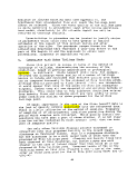 Conclusions Regarding Adequacy of Wastewater Treatment with
Respect to Meeting New Source Performance Standards
The overall conclusion with respect to the adequacy of
wastewater treatment is that the tailings impoundment alone would
not provide treatment that would be adequate to meet EPA's New
Source Performance Standards at the point of discharge "to
Gastineau Channel.
Projections of effluent quality are based in large part on
concentrations of chemical parameters in the influent to the
tailings impoundment. The influent values were derived from
analyses of AJ mine tailings produced during pilot scale milling.
Two water quality models, WASP4 and CE-QUAL-W2, were used to
simulate the processes that would occur in the tailings
impoundment, as suspended particles settle and as metals are
partitioned between solid and dissolved phases.
Table 16 compares projected effluent quality from WASP4 and
CE-QUAL-W2 water quality modeling with EPA's New Source
Performance Standards that would apply to the discharge from this
project. The water quality model results are presented as a
range for both the WASP4 and CE-QUAL-W2 simulations. The ranges
reflect different assumptions used in the scenarios that were
modeled.
Bold numbers indicate those NSPS parameters that are
predicted to be exceeded in the discharge. These include copper
and TSS and possibly mercury, which the CE-QUAL-W2 model
indicates would be exceeded approximately 5% of the time.
Average monthly copper limits would be exceeded under all
scenarios as would TSS when particle settling velocities are
determined according to Stokes1 Law (scenarios 1-12 for the WASP4
model and scenarios C-l and C-2 for the CE-QUAL-W2 simulations).
When zone settling velocities are used (CE-QUAL-W2 scenarios C-3
and C-4), TSS is still predicted to exceed limits during Stage I
operations at least 5% of the time.
86
image:
Conclusions Regarding Adequacy of Wastewater Treatment with
Respect to Meeting New Source Performance Standards
The overall conclusion with respect to the adequacy of
wastewater treatment is that the tailings impoundment alone would
not provide treatment that would be adequate to meet EPA's New
Source Performance Standards at the point of discharge "to
Gastineau Channel.
Projections of effluent quality are based in large part on
concentrations of chemical parameters in the influent to the
tailings impoundment. The influent values were derived from
analyses of AJ mine tailings produced during pilot scale milling.
Two water quality models, WASP4 and CE-QUAL-W2, were used to
simulate the processes that would occur in the tailings
impoundment, as suspended particles settle and as metals are
partitioned between solid and dissolved phases.
Table 16 compares projected effluent quality from WASP4 and
CE-QUAL-W2 water quality modeling with EPA's New Source
Performance Standards that would apply to the discharge from this
project. The water quality model results are presented as a
range for both the WASP4 and CE-QUAL-W2 simulations. The ranges
reflect different assumptions used in the scenarios that were
modeled.
Bold numbers indicate those NSPS parameters that are
predicted to be exceeded in the discharge. These include copper
and TSS and possibly mercury, which the CE-QUAL-W2 model
indicates would be exceeded approximately 5% of the time.
Average monthly copper limits would be exceeded under all
scenarios as would TSS when particle settling velocities are
determined according to Stokes1 Law (scenarios 1-12 for the WASP4
model and scenarios C-l and C-2 for the CE-QUAL-W2 simulations).
When zone settling velocities are used (CE-QUAL-W2 scenarios C-3
and C-4), TSS is still predicted to exceed limits during Stage I
operations at least 5% of the time.
86
image:
 Table 16: Comparison of Projected Effluent Quality and New Source Performance Standards
Parameter
Cadmium
Copper
Lead
Mercury
Zinc
TSS (mg/1)
TSS1 (mg/1)
WASP4 (ug/1
except TSS) )
LOW
9.0
240
150
0.28
410
760
HIGH
19.6
480
940
0.53
940
1800
CE-QUAL-W2 (ug/1
except TSS) )
50%
4.7/6.4
218/242
67.9/102.0
.581/.550
184/273
328/429
0/0
95%
8.0/14.4
395/599
114/223
1.13/1.53
309/600
552/1090
0/44
New Source Peformance
Standards
Maximum
Daily Limit
(ug/1
except TSS)
100
300
600
2
1500
30 mg/1
30 mg/1
Average
Monthly
Limit
(ug/1
except TSS)
50
150
300
1. 0
750
20 mg/1
20 mg/1
1 CE-QUAL-W2 projections using zone settling numbers
87
image:
Table 16: Comparison of Projected Effluent Quality and New Source Performance Standards
Parameter
Cadmium
Copper
Lead
Mercury
Zinc
TSS (mg/1)
TSS1 (mg/1)
WASP4 (ug/1
except TSS) )
LOW
9.0
240
150
0.28
410
760
HIGH
19.6
480
940
0.53
940
1800
CE-QUAL-W2 (ug/1
except TSS) )
50%
4.7/6.4
218/242
67.9/102.0
.581/.550
184/273
328/429
0/0
95%
8.0/14.4
395/599
114/223
1.13/1.53
309/600
552/1090
0/44
New Source Peformance
Standards
Maximum
Daily Limit
(ug/1
except TSS)
100
300
600
2
1500
30 mg/1
30 mg/1
Average
Monthly
Limit
(ug/1
except TSS)
50
150
300
1. 0
750
20 mg/1
20 mg/1
1 CE-QUAL-W2 projections using zone settling numbers
87
image:
 VII. POTENTIAL EFFECTS OF THE DISCHARGE ON WATER QUALITY IN
GASTINEAD CHANNEL
A. Introduction
This portion of the TAR focuses on the potential impacts to
water quality in Gastineau Channel due to wastewater discharges
from the AJ mine and tailings impoundment. • The central question
is whether there is adequate mixing in Gastineau Channel to
dilute the pollutants in the impoundment effluent to ecologically
safe levels. In this chapter, EPA reviews the available
information related to mixing properties in Gastineau Channel and
constructs a model to predict impacts to the channel from the
proposed impoundment discharges.
B. Area Description
Physical Characteristics
Gastineau Channel is a coastal plain estuary which is
partially stratified in the summer and well-mixed during the
winter.
The area is located in southeast Alaska between 58°20' and
58° 10' latitude and 134° 15' and 134° 24'. The channel is a tidal
inlet and is an extension of Stephens Passage. Juneau is located
at the head of the channel (Figure 25) . The entrance to
Gastineau Channel is 4 kilometers west of the convergence of Taku
Inlet and Stephens Passage. At the upstream end of the estuary,
a small navigation channel, passable only at high tide, connects
the tide flats of Gastineau Channel to those of Fitz Cove.
Mel.twater from Mendenhall Glacier and Lemon Creek flows through
these tidal flats into Gastineau Channel, to the southeast, and
Fitz Cove to the west.
The channel is approximately 14 kilometers long from the
mouth at Stephens Passage to the Juneau-Douglas bridge. The
width varies from a minimum of 182 meters at the Juneau bridge to
a maximum of 1,300 meters. The width of over 90% of the channel
is approximately 1,200 meters. The bottom of the channel is
relatively flat, the depth varies from 70 meters at the mouth to
20 meters near Juneau. Over 90% of the channel the depth varies
only slightly from the average channel depth of 38 meters.
Topography surrounding the channel is characterized as
steep, glacially- carved valleys to the east, with elevations
ranging from sea level at the channel to 1,200 meters in the
glacial areas. Glaciers surrounding the channel provide a
continual freshwater source due to meltwater during summer
months. The steep hills of Douglas Island border the channel to
the west.
88
image:
VII. POTENTIAL EFFECTS OF THE DISCHARGE ON WATER QUALITY IN
GASTINEAD CHANNEL
A. Introduction
This portion of the TAR focuses on the potential impacts to
water quality in Gastineau Channel due to wastewater discharges
from the AJ mine and tailings impoundment. • The central question
is whether there is adequate mixing in Gastineau Channel to
dilute the pollutants in the impoundment effluent to ecologically
safe levels. In this chapter, EPA reviews the available
information related to mixing properties in Gastineau Channel and
constructs a model to predict impacts to the channel from the
proposed impoundment discharges.
B. Area Description
Physical Characteristics
Gastineau Channel is a coastal plain estuary which is
partially stratified in the summer and well-mixed during the
winter.
The area is located in southeast Alaska between 58°20' and
58° 10' latitude and 134° 15' and 134° 24'. The channel is a tidal
inlet and is an extension of Stephens Passage. Juneau is located
at the head of the channel (Figure 25) . The entrance to
Gastineau Channel is 4 kilometers west of the convergence of Taku
Inlet and Stephens Passage. At the upstream end of the estuary,
a small navigation channel, passable only at high tide, connects
the tide flats of Gastineau Channel to those of Fitz Cove.
Mel.twater from Mendenhall Glacier and Lemon Creek flows through
these tidal flats into Gastineau Channel, to the southeast, and
Fitz Cove to the west.
The channel is approximately 14 kilometers long from the
mouth at Stephens Passage to the Juneau-Douglas bridge. The
width varies from a minimum of 182 meters at the Juneau bridge to
a maximum of 1,300 meters. The width of over 90% of the channel
is approximately 1,200 meters. The bottom of the channel is
relatively flat, the depth varies from 70 meters at the mouth to
20 meters near Juneau. Over 90% of the channel the depth varies
only slightly from the average channel depth of 38 meters.
Topography surrounding the channel is characterized as
steep, glacially- carved valleys to the east, with elevations
ranging from sea level at the channel to 1,200 meters in the
glacial areas. Glaciers surrounding the channel provide a
continual freshwater source due to meltwater during summer
months. The steep hills of Douglas Island border the channel to
the west.
88
image:
 SHEEP CREEK
TAILINGS DISPOSAL OPTION
sg^^t^n /?,3e?^i
/%. •.. ^\••• •! /i i':<r\i'c5C.'i««
Figure 25 : Project Area
Source: Echo Bay Alaska, Inc.
image:
SHEEP CREEK
TAILINGS DISPOSAL OPTION
sg^^t^n /?,3e?^i
/%. •.. ^\••• •! /i i':<r\i'c5C.'i««
Figure 25 : Project Area
Source: Echo Bay Alaska, Inc.
image:
 2. Meteorology
Juneau is located in a coastal zone region with maritime
climate. The climate is affected by storms which originate in or
cross the Gulf of Alaska in a general westerly direction. Due to
the moderating effects of the maritime climate, temperatures are
mild for this latitude.
There is moderate variation in daily and seasonal
temperatures in the Juneau area. Monthly average temperatures
range from 28°F in January to 57°F in July.
This area receives an abundant amount of precipitation with
a total annual average of 90 inches. The lowest monthly
precipitation occurs in June, with an average of 4 inches at the
downtown station. The maximum average monthly precipitation
occurs in October (13 inches).
Due to the orographic effects precipitation varies greatly
over short distances. The quantity of precipitation increases
sharply with elevation to the east of Juneau. At Juneau Ice
Field, 30 miles east of Juneau, the estimated annual
precipitation is 200 inches.
Snowfall at the downtown station averages over 79 inches
annually. Semi-permanent snowfields are found at elevations of
3.300 feet on the north-facing slopes of Roberts Peak and Sheep
Mountain.
Surface winds are strongly channeled by the steep terrain.
Gastineau Channel is oriented northwest-southeast, the same
direction as the surface winds. Wind observations from the
downtown station indicate that southeast winds occur 65 percent
of the time and northwest winds occur 15 percent of the time.
The mean annual wind speed from the airport station records
indicate an annual mean wind speed of 3.7 meters per second. The
monthly means range from 3.3 m/s in August to 4.3 m/s in October.
There is less channelization of wind at the-airport (northeast of
town) than downtown (near the channel). Short periods of strong
gusty northerly or easterly winds occur during the winter months.
3. Freshwater Sources
A number of creeks provide freshwater to the surface layer
of Gastineau Channel. U.S. Geological Service (USGS) streamflow
records are available for Gold Creek, Sheep Creek and Lawson
Creek. Gold Creek has been gauged from 1918-1982 and 1985-
present, Sheep Creek for the period of 1919-1973, and Lawson
Creek 1970-1971.
90
image:
2. Meteorology
Juneau is located in a coastal zone region with maritime
climate. The climate is affected by storms which originate in or
cross the Gulf of Alaska in a general westerly direction. Due to
the moderating effects of the maritime climate, temperatures are
mild for this latitude.
There is moderate variation in daily and seasonal
temperatures in the Juneau area. Monthly average temperatures
range from 28°F in January to 57°F in July.
This area receives an abundant amount of precipitation with
a total annual average of 90 inches. The lowest monthly
precipitation occurs in June, with an average of 4 inches at the
downtown station. The maximum average monthly precipitation
occurs in October (13 inches).
Due to the orographic effects precipitation varies greatly
over short distances. The quantity of precipitation increases
sharply with elevation to the east of Juneau. At Juneau Ice
Field, 30 miles east of Juneau, the estimated annual
precipitation is 200 inches.
Snowfall at the downtown station averages over 79 inches
annually. Semi-permanent snowfields are found at elevations of
3.300 feet on the north-facing slopes of Roberts Peak and Sheep
Mountain.
Surface winds are strongly channeled by the steep terrain.
Gastineau Channel is oriented northwest-southeast, the same
direction as the surface winds. Wind observations from the
downtown station indicate that southeast winds occur 65 percent
of the time and northwest winds occur 15 percent of the time.
The mean annual wind speed from the airport station records
indicate an annual mean wind speed of 3.7 meters per second. The
monthly means range from 3.3 m/s in August to 4.3 m/s in October.
There is less channelization of wind at the-airport (northeast of
town) than downtown (near the channel). Short periods of strong
gusty northerly or easterly winds occur during the winter months.
3. Freshwater Sources
A number of creeks provide freshwater to the surface layer
of Gastineau Channel. U.S. Geological Service (USGS) streamflow
records are available for Gold Creek, Sheep Creek and Lawson
Creek. Gold Creek has been gauged from 1918-1982 and 1985-
present, Sheep Creek for the period of 1919-1973, and Lawson
Creek 1970-1971.
90
image:
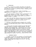 To estimate the total freshwater discharge into the channel,
Echo Bay used information from the gauged streams to estimate the
total freshwater discharge into the channel (Andrews, 1991). To
determine the total flows into the channel, discharge from the
areas not represented by historic USGS gauged stations were
estimated.
To obtain the estimates for ungauged areas, a discharge rate
per unit drainage area was determined for each area based on USGS
flow and drainage area records. These values were then
multiplied by the ungauged areas with similar topography. The
Gold Creek drainage value was used to determine the discharge for
the Salmon Creek and Snowslide/Cross Bay area, the Sheep Creek
value for Little Sheep/Dupont area, and the Lawson Creek value
for the Douglas Island area.
Relative discharge contributions for each creek to the total
flow are summarized below.
Table 17: Basin Contributions
Basin
Gold Creek
Salmon Creek
Cross Bay/Snowslide Creek
Sheep Creek
Little Sheep/Dupont Creek
Douglas Island
Percent Contribution to
Channel
27%
25%
12%
16%
16%
4%
Flowrates for the above basins vary significantly over the
seasons. Generally, low flows occur in winter months (November -
April) while higher flows occur in the summer months (June -
October) . For example, average July flows in Gold Creek are ten
times higher than average March flows (Comprehensive Report,
Table 3-4; EBA, 1992).
4_._ Tidal Influence
Gastineau Channel is not connected directly to the open
marine waters of the Pacific Ocean. Rather, the channel is
influenced by adjoining channels, which provide a source of
freshwater to the channel. The tides in this area are
semidiurnal unequal, with a period of approximately 12.4 hours
The mean tidal height is 2.5 meters with an average wave height
of 3.5 meters.
91
image:
To estimate the total freshwater discharge into the channel,
Echo Bay used information from the gauged streams to estimate the
total freshwater discharge into the channel (Andrews, 1991). To
determine the total flows into the channel, discharge from the
areas not represented by historic USGS gauged stations were
estimated.
To obtain the estimates for ungauged areas, a discharge rate
per unit drainage area was determined for each area based on USGS
flow and drainage area records. These values were then
multiplied by the ungauged areas with similar topography. The
Gold Creek drainage value was used to determine the discharge for
the Salmon Creek and Snowslide/Cross Bay area, the Sheep Creek
value for Little Sheep/Dupont area, and the Lawson Creek value
for the Douglas Island area.
Relative discharge contributions for each creek to the total
flow are summarized below.
Table 17: Basin Contributions
Basin
Gold Creek
Salmon Creek
Cross Bay/Snowslide Creek
Sheep Creek
Little Sheep/Dupont Creek
Douglas Island
Percent Contribution to
Channel
27%
25%
12%
16%
16%
4%
Flowrates for the above basins vary significantly over the
seasons. Generally, low flows occur in winter months (November -
April) while higher flows occur in the summer months (June -
October) . For example, average July flows in Gold Creek are ten
times higher than average March flows (Comprehensive Report,
Table 3-4; EBA, 1992).
4_._ Tidal Influence
Gastineau Channel is not connected directly to the open
marine waters of the Pacific Ocean. Rather, the channel is
influenced by adjoining channels, which provide a source of
freshwater to the channel. The tides in this area are
semidiurnal unequal, with a period of approximately 12.4 hours
The mean tidal height is 2.5 meters with an average wave height
of 3.5 meters.
91
image:
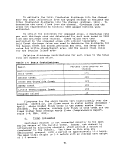 C. Previous Studies
Several field studies have been conducted to assess the
capacity of the channel to provide dispersion and dilution of
waste discharges. The following discussion and analysis briefly
summarize data presented in these field reports.
1. Sewage Outfall Study 1965
One of the first studies conducted in the channel was
conducted in August 1965. The purpose of this study was to
evaluate the placement of the city's sewage outfall.
Investigations were conducted mainly in the area near the Juneau-
Douglas Island Bridge. This site was investigated because
observed turbulence in this region suggested that it might
provide additional mixing capacity. Measurements of temperature,
salinity, dissolved oxygen and pH were obtained. A plot of the
longitudinal salinity distribution near high water slack is shown
in Figure 26.
Current float studies were conducted at various depths and
locations during both flood and ebb tides. A rhodamine dye
tracer was released at the water surface under the bridge during
a flood tide on August 17 and during an ebb tide on August 20.
Several rip tides were observed in the vicinity of the bridge.
These tides were observed above the bridge during the flood tide
and below the bridge during the ebb. Surface dye was observed
sinking, at the rip tide area.
2. Seawater Monitoring 1989 - 1990
Salinity is an important element in the analysis of
estuaries, because salt can be treated as a conservative tracer,
descriptive of the mixing characteristics of the waterbody.
Salinity levels also describe a waterbody's vertical density
stratification, which is an important element of discharge plume
dynamics. Echo Bay conducted a seawater monitoring program
during the months of May 1989, September 1989, March 1990, August
1990, -and September 1990. Salinity and temperature profiles were
obtained during single excursions for a given month. Salinity
data for September 1989 and March 1990 are included in Appendix
Dl.
3. Channel Current Survey 1990
During the summer months, Echo Bay conducted a current
survey near Thane and the Rock Dump Site (see Appendix D3). The
mooring at the Thane site was deployed in 30 meters of water,
with current meters at 12, 19 and 26 meter depths. This meter
was operated from June 29, 1990, to July 21, 1990. The mooring
at the Rock Dump site was deployed in 24 meters of water and
operated from June 29, 1990 to August 28, 1990, with current
92
image:
C. Previous Studies
Several field studies have been conducted to assess the
capacity of the channel to provide dispersion and dilution of
waste discharges. The following discussion and analysis briefly
summarize data presented in these field reports.
1. Sewage Outfall Study 1965
One of the first studies conducted in the channel was
conducted in August 1965. The purpose of this study was to
evaluate the placement of the city's sewage outfall.
Investigations were conducted mainly in the area near the Juneau-
Douglas Island Bridge. This site was investigated because
observed turbulence in this region suggested that it might
provide additional mixing capacity. Measurements of temperature,
salinity, dissolved oxygen and pH were obtained. A plot of the
longitudinal salinity distribution near high water slack is shown
in Figure 26.
Current float studies were conducted at various depths and
locations during both flood and ebb tides. A rhodamine dye
tracer was released at the water surface under the bridge during
a flood tide on August 17 and during an ebb tide on August 20.
Several rip tides were observed in the vicinity of the bridge.
These tides were observed above the bridge during the flood tide
and below the bridge during the ebb. Surface dye was observed
sinking, at the rip tide area.
2. Seawater Monitoring 1989 - 1990
Salinity is an important element in the analysis of
estuaries, because salt can be treated as a conservative tracer,
descriptive of the mixing characteristics of the waterbody.
Salinity levels also describe a waterbody's vertical density
stratification, which is an important element of discharge plume
dynamics. Echo Bay conducted a seawater monitoring program
during the months of May 1989, September 1989, March 1990, August
1990, -and September 1990. Salinity and temperature profiles were
obtained during single excursions for a given month. Salinity
data for September 1989 and March 1990 are included in Appendix
Dl.
3. Channel Current Survey 1990
During the summer months, Echo Bay conducted a current
survey near Thane and the Rock Dump Site (see Appendix D3). The
mooring at the Thane site was deployed in 30 meters of water,
with current meters at 12, 19 and 26 meter depths. This meter
was operated from June 29, 1990, to July 21, 1990. The mooring
at the Rock Dump site was deployed in 24 meters of water and
operated from June 29, 1990 to August 28, 1990, with current
92
image:
 Juneau-Douglas
Bridge
0"
Nautical Miles From Bridge
_}_
i
_6_
l
CO
u
10
20
z 30
I
a,
UJ
a so
-J2,ft
*r,u
- /tV
BOTTOM OF GASTINEAU CHANNEL
Figure 26 : Observed Pattern of Salinity in Gastineau Channel Near High-Water Slack
on August 20, 1965.
(U.S. Department of Interior, 1966)
STCPHENS
PASSAGE
image:
Juneau-Douglas
Bridge
0"
Nautical Miles From Bridge
_}_
i
_6_
l
CO
u
10
20
z 30
I
a,
UJ
a so
-J2,ft
*r,u
- /tV
BOTTOM OF GASTINEAU CHANNEL
Figure 26 : Observed Pattern of Salinity in Gastineau Channel Near High-Water Slack
on August 20, 1965.
(U.S. Department of Interior, 1966)
STCPHENS
PASSAGE
image:
 meters located .at 13, 17 and 22 meter depths. Temperature,
conductivity, current speed and direction were measured at 15
minute intervals. During the period of August 27 to August 30,
drogued buoys were deployed near the Thane site during both flood
and ebb condition. The buoys were drogued at a depth of 1.5
meters, except on August 30 when the drogue was changed to a 5
meter depth.
4. Thane Current Survey 1992
One current meter was deployed at the Thane site (see
Appendix D3) for the period of February 18 through April 24,
1992. Current meters were located at depths of 5, 10, 20 and 30
meters. In addition to measuring current speed, temperature and
salinity information were obtained. Drift buoys drogued at 1.5
and 3 meters and surface drifters were also deployed on two days
during this survey (see Appendix D9).
Drift Card Study 1992
A drift card study was conducted by the National Marine
Fisheries Service (NMFS) Auke Bay Laboratory in May 1992. The
purpose of this study was to evaluate salmon fry migration over
Mendenhall bar. Two thousand drift cards were released at three
different locations in Gastineau Channel. The cards were
released on ebb and flood tides on two different days. Appendix
D9 contains the location and percent recovered for corresponding
release stations.
6. Study Summaries and Comparison
a. Surface Flow Characteristics
i. Winter
NMFS1 drift card study was conducted in May 1992. A
majority of the cards released in Gastineau Channel remained in
the channel, indicating a limited degree of communication between
the surface of Gastineau Channel and Fitz Cove to the north.
Echo Bay's drift surveys in 1992 indicate some influence of
winds on surface flows. Under steady north winds during an ebb
tide on March 31, buoys were driven to the Douglas Island
shoreline and then slightly up-channel to the northwest.
Meanwhile, buoys at 1.5 and 10 meter depths travelled southeast
in accordance with the expected tidal current.
Under southeast winds during a flood tide on April 23,
bouys at all depths travelled northwest in the direction of the
tidal current. The travel distance for buoys at the 10 meter
depth was relatively short, while the surface buoys travelled as
far as the rock dump area.
94
image:
meters located .at 13, 17 and 22 meter depths. Temperature,
conductivity, current speed and direction were measured at 15
minute intervals. During the period of August 27 to August 30,
drogued buoys were deployed near the Thane site during both flood
and ebb condition. The buoys were drogued at a depth of 1.5
meters, except on August 30 when the drogue was changed to a 5
meter depth.
4. Thane Current Survey 1992
One current meter was deployed at the Thane site (see
Appendix D3) for the period of February 18 through April 24,
1992. Current meters were located at depths of 5, 10, 20 and 30
meters. In addition to measuring current speed, temperature and
salinity information were obtained. Drift buoys drogued at 1.5
and 3 meters and surface drifters were also deployed on two days
during this survey (see Appendix D9).
Drift Card Study 1992
A drift card study was conducted by the National Marine
Fisheries Service (NMFS) Auke Bay Laboratory in May 1992. The
purpose of this study was to evaluate salmon fry migration over
Mendenhall bar. Two thousand drift cards were released at three
different locations in Gastineau Channel. The cards were
released on ebb and flood tides on two different days. Appendix
D9 contains the location and percent recovered for corresponding
release stations.
6. Study Summaries and Comparison
a. Surface Flow Characteristics
i. Winter
NMFS1 drift card study was conducted in May 1992. A
majority of the cards released in Gastineau Channel remained in
the channel, indicating a limited degree of communication between
the surface of Gastineau Channel and Fitz Cove to the north.
Echo Bay's drift surveys in 1992 indicate some influence of
winds on surface flows. Under steady north winds during an ebb
tide on March 31, buoys were driven to the Douglas Island
shoreline and then slightly up-channel to the northwest.
Meanwhile, buoys at 1.5 and 10 meter depths travelled southeast
in accordance with the expected tidal current.
Under southeast winds during a flood tide on April 23,
bouys at all depths travelled northwest in the direction of the
tidal current. The travel distance for buoys at the 10 meter
depth was relatively short, while the surface buoys travelled as
far as the rock dump area.
94
image:
 11.
Summer
Five deployments were made during ebb and flood tide during
the period of August 27 to August 30, 1990. All buoys recovered
during the August 1990 deployment were recovered further up-
channel from the location they started. For these deployments,
transport was up-channel during high winds (10-15 knots) and
followed the expected tidal current during calm periods.
b. Channel Flow Properties
i. Winter
Mean current speeds in March 1992 at Thane are summarized in
Table 18. Residual, along-channel velocities for the period are
presented graphically in Figure 27. The depth at which the
velocity profile changes direction is approximately 10 meters
below the surface. Based on Table 19 the average residual
velocity in the upper 10 meters is approximately .8 cm/sec, in
the down-channel direction. The average residual velocity for
the lower layer 20 meters is approximately .5 cm/sec, in the up-
channel direction.
Table 18: Average Current Speeds at Thane in March 1992
Depth (m)
5
10
20
30
Avg Velocity
(cm/ sec)
11.9
9.1
7.4
7.6
11.
Summer
Average current velocities in March 1992 at Thane are
summarized in Table 19. The average residual velocities for the
June to August 1990 investigation are listed in Table 19. The
residual data for Station A would suggest that there is a net
flow down-channel at all depths; however, the surface layer of
the estuary was not monitored. The up-channel flow at the
shallowest meter monitored (Station B, 11.5 meters) suggests that
measurements were generally obtained below a down-channel flow in
the surface layer.
95
image:
11.
Summer
Five deployments were made during ebb and flood tide during
the period of August 27 to August 30, 1990. All buoys recovered
during the August 1990 deployment were recovered further up-
channel from the location they started. For these deployments,
transport was up-channel during high winds (10-15 knots) and
followed the expected tidal current during calm periods.
b. Channel Flow Properties
i. Winter
Mean current speeds in March 1992 at Thane are summarized in
Table 18. Residual, along-channel velocities for the period are
presented graphically in Figure 27. The depth at which the
velocity profile changes direction is approximately 10 meters
below the surface. Based on Table 19 the average residual
velocity in the upper 10 meters is approximately .8 cm/sec, in
the down-channel direction. The average residual velocity for
the lower layer 20 meters is approximately .5 cm/sec, in the up-
channel direction.
Table 18: Average Current Speeds at Thane in March 1992
Depth (m)
5
10
20
30
Avg Velocity
(cm/ sec)
11.9
9.1
7.4
7.6
11.
Summer
Average current velocities in March 1992 at Thane are
summarized in Table 19. The average residual velocities for the
June to August 1990 investigation are listed in Table 19. The
residual data for Station A would suggest that there is a net
flow down-channel at all depths; however, the surface layer of
the estuary was not monitored. The up-channel flow at the
shallowest meter monitored (Station B, 11.5 meters) suggests that
measurements were generally obtained below a down-channel flow in
the surface layer.
95
image:
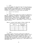 ft
0
-5
-10
£
o -20
.-25
-30
-35
-•• r • i — i • i —
\
/
i
\
\
\
1
X
'
\
.5
3
Speed
*
,
i
5
(cm/s)
"
•
i
i
I 1 1 • »—
1 1
I
5 2
Figure 27 :
Residual along-chnniicl velocity profile Tor period 18 February to
24 April 1992
Source: Comprehensive Report
image:
ft
0
-5
-10
£
o -20
.-25
-30
-35
-•• r • i — i • i —
\
/
i
\
\
\
1
X
'
\
.5
3
Speed
*
,
i
5
(cm/s)
"
•
i
i
I 1 1 • »—
1 1
I
5 2
Figure 27 :
Residual along-chnniicl velocity profile Tor period 18 February to
24 April 1992
Source: Comprehensive Report
image:
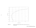 Table 19 Average Current Speeds for June - August 1990
Station A
Depth (m)
13.5
17.0
22.1
Velocity
cm/ sec
5.3
5.0
2.2
Station B
Depth (m)
11.5
19.0
26.5
Velocity
cm/ sec
8.7
4.4
4.7
Table 20 Average Residual Current Velocity June - August 1990
Station A
Depth (m)
13.5
17.0
22.1
Velocity
cm/ sec
2.1
1.6
0.7
Station B
Depth (m)
11.5
19.0
26.5
Velocity
cm/ sec
-1.8
0.5
0.8
(negative values represent down channel flow)
c. Salinity Distributions
Winter
Observations of salinity reported in the seawater monitoring
report indicate a minimal amount of stratification for the period
between November and March. For March 1991, the average salinity
for stations near the mouth was 31 ppt. The average salinity for
stations up channel .was 29 ppt. The March 1990 records indicate
an average salinity of 29 ppt, with this value relatively uniform
up-channel. The November profile indicates an average salinity of
31 ppt near the mouth, and an average up-hannel salinity of 29
ppt.
Salinity profiles obtained during the February-April 1992
investigation indicate a relatively uniform profile for February
with an average salinity of 30.2 ppt. The March and April
profiles indicate a stratified layer with increased surface
temperatures. It appears that over the data collection period of
February 18 - April 24, 1992, stratification was increasing. This
increasing degree of stratification was probably due to an
increase in freshwater flows. The monthly average freshwater flow
for Gold Creek for March 1992 was 68 cfs, which is over 5 times
greater than the long-term average March flow.
97
image:
Table 19 Average Current Speeds for June - August 1990
Station A
Depth (m)
13.5
17.0
22.1
Velocity
cm/ sec
5.3
5.0
2.2
Station B
Depth (m)
11.5
19.0
26.5
Velocity
cm/ sec
8.7
4.4
4.7
Table 20 Average Residual Current Velocity June - August 1990
Station A
Depth (m)
13.5
17.0
22.1
Velocity
cm/ sec
2.1
1.6
0.7
Station B
Depth (m)
11.5
19.0
26.5
Velocity
cm/ sec
-1.8
0.5
0.8
(negative values represent down channel flow)
c. Salinity Distributions
Winter
Observations of salinity reported in the seawater monitoring
report indicate a minimal amount of stratification for the period
between November and March. For March 1991, the average salinity
for stations near the mouth was 31 ppt. The average salinity for
stations up channel .was 29 ppt. The March 1990 records indicate
an average salinity of 29 ppt, with this value relatively uniform
up-channel. The November profile indicates an average salinity of
31 ppt near the mouth, and an average up-hannel salinity of 29
ppt.
Salinity profiles obtained during the February-April 1992
investigation indicate a relatively uniform profile for February
with an average salinity of 30.2 ppt. The March and April
profiles indicate a stratified layer with increased surface
temperatures. It appears that over the data collection period of
February 18 - April 24, 1992, stratification was increasing. This
increasing degree of stratification was probably due to an
increase in freshwater flows. The monthly average freshwater flow
for Gold Creek for March 1992 was 68 cfs, which is over 5 times
greater than the long-term average March flow.
97
image:
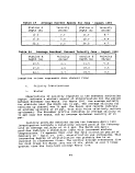 ii. Summer
Profiles for the summer period were available for August
1990 and September 1989. The August profiles show a distinct
stratification extending to a depth of approximately 10 meters.
The minimum salinity observed in the surface layer was 9 ppt.
Salinity in the surface layer appears to increase in the up-
channel direction. This phenomenon was also observed in salinity
data from the 1965 study. The September 1989 profiles show a
similar trend, with a stratified layer extending to a depth of 10
meters. The September data exhibits the same increase in the
surface salinity with up-channel distance.
Salinity data from the June-August 1990 current mooring were
obtained at depths generally below the stratified layer. The
shallowest meter was located at a depth of 12 meters.
7. Physical Description Summary &. Interpretation
In summary, there appear to be two distinct periods and
mixing conditions in Gastineau .Channel. The winter period
between November and March is characterized by relatively low
freshwater tributary input, colder surface layer, and well mixed
vertical conditions.
The summer period, between April and September, may be
characterized by a five-fold increase in tributary inflow, a
stratified upper layer consisting of less saline and warmer
water, and an increase in salinity in the upper layer in the up-
channel direction. The period of maximum stratification appears
to coincide with the maximum glacier melt and subsequent runoff.
Based on the pattern of salinity increasing in the up-channel
direction, it appears a significant portion of the freshwater
entering the channel during the summer period originates in
Stephens Passage.
The general circulation observed during both winter and
summer periods is directed up-channel (towards Juneau) at depth
and down-channel in the upper layer. During periods of high
winds, surface currents are enhanced either in the down- or up-
channel surface flows. The predominant direction would appear to
be up-channel influence due to the frequency of the up-channel
wind occurrences (65%). This effect may explain the March 1992
drift buoys moving up-channel at the surface and down-channel
below 1.5 meters.
The primary mixing mechanisms for an estuarine system
identified by Ippen (1966) include: a) the effect of the tide; b)
the effect of gravitational forces due to density variations
between freshwater from upland sources and saline water from the
sea; c) the gravitational force needed to produce a net seaward
transport of freshwater; and d.) the Coriolis forces and
98
image:
ii. Summer
Profiles for the summer period were available for August
1990 and September 1989. The August profiles show a distinct
stratification extending to a depth of approximately 10 meters.
The minimum salinity observed in the surface layer was 9 ppt.
Salinity in the surface layer appears to increase in the up-
channel direction. This phenomenon was also observed in salinity
data from the 1965 study. The September 1989 profiles show a
similar trend, with a stratified layer extending to a depth of 10
meters. The September data exhibits the same increase in the
surface salinity with up-channel distance.
Salinity data from the June-August 1990 current mooring were
obtained at depths generally below the stratified layer. The
shallowest meter was located at a depth of 12 meters.
7. Physical Description Summary &. Interpretation
In summary, there appear to be two distinct periods and
mixing conditions in Gastineau .Channel. The winter period
between November and March is characterized by relatively low
freshwater tributary input, colder surface layer, and well mixed
vertical conditions.
The summer period, between April and September, may be
characterized by a five-fold increase in tributary inflow, a
stratified upper layer consisting of less saline and warmer
water, and an increase in salinity in the upper layer in the up-
channel direction. The period of maximum stratification appears
to coincide with the maximum glacier melt and subsequent runoff.
Based on the pattern of salinity increasing in the up-channel
direction, it appears a significant portion of the freshwater
entering the channel during the summer period originates in
Stephens Passage.
The general circulation observed during both winter and
summer periods is directed up-channel (towards Juneau) at depth
and down-channel in the upper layer. During periods of high
winds, surface currents are enhanced either in the down- or up-
channel surface flows. The predominant direction would appear to
be up-channel influence due to the frequency of the up-channel
wind occurrences (65%). This effect may explain the March 1992
drift buoys moving up-channel at the surface and down-channel
below 1.5 meters.
The primary mixing mechanisms for an estuarine system
identified by Ippen (1966) include: a) the effect of the tide; b)
the effect of gravitational forces due to density variations
between freshwater from upland sources and saline water from the
sea; c) the gravitational force needed to produce a net seaward
transport of freshwater; and d.) the Coriolis forces and
98
image:
 centrifugal forces inducing transverse fluid motion due. to the
rotation of the earth and any curvature of the estuary. From the
above physical description of the Gastineau Channel system, the
primary mixing mechanisms at work are the tides, the seaward
transport of freshwater, and wind-driven advection at the
surface.
D. Screening Analysis for Water Quality Impacts
1. Analysis by Echo Bay Alaska
Analyses provided by Echo Bay have employed the use of a
single cell or "box" model to assert that long-term (or far-
field) mixing is not significantly limited. A diagram of the
single cell concept is shown in Figure 28. If this far-field
mixing is assured, near-field dilution modeling would be useful
in ascertaining the dimensions and dilution in any mixing zone
(Comprehensive Report; EBA, 1992).
For a number of reasons, the box model described in the
Comprehensive Report does not represent a worst-case view of the
far-field impacts. First, this model does not address the
potential for stratification to trap the discharge plume in the
lower waters of the channel, which tend to migrate up-channel.
Another problem stems from the use of average current speeds,
artificially set in one direction, to move water into the
channel. Residual currents are a more appropriate measure of
minimum net transport into and out of a waterbody over time,
because residual currents represent the net current after the
flow reversal effect of tidal currents is filtered out of the
data. Finally, the box model assumes that all waters within the
box are mixed instantaneously, which neglects the potential for
relatively higher impacts in the upper channel than in the lower
channel due to relative distances from the tidal source (Stephens
Passage).
2. Alternative Screening Analysis
As background to conducting a more detailed analysis of
mixing in Gastineau Channel, EPA used the residual current speed
documented in the Comprehensive Report (Figure 27) to estimate
the available dilution flows at a given site in the channel. In
this case, EPA compared the projected effluent flow from the AJ
mine with the estimated cross-sectional flow in Gastineau
Channel, calculated as the net flux passing through the channel
cross-section by virtue of the residual current (Figure 29).
99
image:
centrifugal forces inducing transverse fluid motion due. to the
rotation of the earth and any curvature of the estuary. From the
above physical description of the Gastineau Channel system, the
primary mixing mechanisms at work are the tides, the seaward
transport of freshwater, and wind-driven advection at the
surface.
D. Screening Analysis for Water Quality Impacts
1. Analysis by Echo Bay Alaska
Analyses provided by Echo Bay have employed the use of a
single cell or "box" model to assert that long-term (or far-
field) mixing is not significantly limited. A diagram of the
single cell concept is shown in Figure 28. If this far-field
mixing is assured, near-field dilution modeling would be useful
in ascertaining the dimensions and dilution in any mixing zone
(Comprehensive Report; EBA, 1992).
For a number of reasons, the box model described in the
Comprehensive Report does not represent a worst-case view of the
far-field impacts. First, this model does not address the
potential for stratification to trap the discharge plume in the
lower waters of the channel, which tend to migrate up-channel.
Another problem stems from the use of average current speeds,
artificially set in one direction, to move water into the
channel. Residual currents are a more appropriate measure of
minimum net transport into and out of a waterbody over time,
because residual currents represent the net current after the
flow reversal effect of tidal currents is filtered out of the
data. Finally, the box model assumes that all waters within the
box are mixed instantaneously, which neglects the potential for
relatively higher impacts in the upper channel than in the lower
channel due to relative distances from the tidal source (Stephens
Passage).
2. Alternative Screening Analysis
As background to conducting a more detailed analysis of
mixing in Gastineau Channel, EPA used the residual current speed
documented in the Comprehensive Report (Figure 27) to estimate
the available dilution flows at a given site in the channel. In
this case, EPA compared the projected effluent flow from the AJ
mine with the estimated cross-sectional flow in Gastineau
Channel, calculated as the net flux passing through the channel
cross-section by virtue of the residual current (Figure 29).
99
image:
 38m
Gold
Creek
Sheep
Creek
A-J
Outfall
•
Stephens
^"r
• " ..• ~
•
.
.
.. • rt
^"^"- "r
&-'£**.'&• ' ' :•••••• 'x-
-\ r~ ~\ i ~\ :
V V V
\
• -- •..-.;.;; ' ' .;.:::-:;v.^ •••••;:•:•:•. •'• --.•;,• - • • • ..;••. .
'" '.-:'"' '..-.. ;;'. ' ''.; -V- 1:'''-' '-'•'' ':' / : .' ':•'' -•"••'•'''• ; ;;- ''::.;- '''•''.'•' : .:•' • '•• • • ' -
•''••"'.•.. : .; ."•;;." ' ''; •'• • •- . •
:' • ?-$&£j$: '"';:';:.:-::-: v:.:.-. v':. -'.•• .. •:...• .:.. ,': • ••••v;'.':': :^:,i§|;i:v^^ •
G A:S;:7: I N'E^A U C H A N N E'L
"• '. •••. . • ' '•'•. -.•*•• .-:.' .•••'• . . ',' , ' .';' •:• " ''.-'.' ' ','•' •••'•-- ' • - : ; : ._: ' . • .
<jj:
^^
Tidal inflow + A-J outfall
+ Sheep Creek + Gold Crce
^4—
/^
<CT Tidal inflow
. ^"\^-
^^ ^\
13,800m
tfp*
Figure 28 : Conceptual Diagram of Single Cell Model
Source: Comprehensive Report
image:
38m
Gold
Creek
Sheep
Creek
A-J
Outfall
•
Stephens
^"r
• " ..• ~
•
.
.
.. • rt
^"^"- "r
&-'£**.'&• ' ' :•••••• 'x-
-\ r~ ~\ i ~\ :
V V V
\
• -- •..-.;.;; ' ' .;.:::-:;v.^ •••••;:•:•:•. •'• --.•;,• - • • • ..;••. .
'" '.-:'"' '..-.. ;;'. ' ''.; -V- 1:'''-' '-'•'' ':' / : .' ':•'' -•"••'•'''• ; ;;- ''::.;- '''•''.'•' : .:•' • '•• • • ' -
•''••"'.•.. : .; ."•;;." ' ''; •'• • •- . •
:' • ?-$&£j$: '"';:';:.:-::-: v:.:.-. v':. -'.•• .. •:...• .:.. ,': • ••••v;'.':': :^:,i§|;i:v^^ •
G A:S;:7: I N'E^A U C H A N N E'L
"• '. •••. . • ' '•'•. -.•*•• .-:.' .•••'• . . ',' , ' .';' •:• " ''.-'.' ' ','•' •••'•-- ' • - : ; : ._: ' . • .
<jj:
^^
Tidal inflow + A-J outfall
+ Sheep Creek + Gold Crce
^4—
/^
<CT Tidal inflow
. ^"\^-
^^ ^\
13,800m
tfp*
Figure 28 : Conceptual Diagram of Single Cell Model
Source: Comprehensive Report
image:
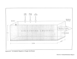 trapping depth
Residual Current
(.005 m/s)
bottom layer
channel cross-section
(25 m x 1300m)
diffuser
effluent plume
Figure 29 : Conceptual Framework for Volume Flux Approach
image:
trapping depth
Residual Current
(.005 m/s)
bottom layer
channel cross-section
(25 m x 1300m)
diffuser
effluent plume
Figure 29 : Conceptual Framework for Volume Flux Approach
image:
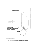 The volume flux, is calculated as follows:
AJ Maximum Discharge Flow = 200 cfs =18.6 m3/sec
Channel Cross Section (below 10 m) = 25 m x 1300 m = 32,500 m2
Avg Residual Current (below 10 m) = .5 cm/sec = .005 m/s
Volume Flux = (Cross section) x (avg residual velocity)
= 32500 x .005 = 162.5 m3/sec
Dilution at Max Flow = (Volume Flux)/(AJ Discharge Flow)
= 162/18.6 = 9
These calculations suggest that flows through the channel at
slack tide (residual currents only) would dilute the effluent by
a factor of 9, significantly less than the estimated initial
dilution of approximately 100:1 described in Echo Bay's
Comprehensive Report. While the tides would be expected to
provide additional dilution in .the system, this contribution
would be expected to dwindle with increased distance from the
channel entrance.
The above screening calculations, coupled with concerns
about the assumptions of the Echo Bay box model, leads EPA to
conclude that the analyses to date do not adequately evaluate the
potential for accumulation of pollutants in the upper part of the
channel. As a result, EPA pursued a more detailed analysis of
the problem using the WASP4 model.
E. Analysis using WASP4 Framework
lj Introduction
The Water Quality Analysis Simulation Program Version 4.32
(Ambrose et al., 1991) is a dynamic compartment modeling system
that has been widely used in the United States to predict water
quality responses to pollution. It simulates transport and
transformation of conventional and toxic pollutants in surface
waters using finite difference techniques. The model is
maintained and supported by the USEPA Center for Exposure
Assessment Modeling in Athens, Georgia.
The WASP4 Model developed for Gastineau Channel was
calibrated using salinity to determine reasonable mixing
conditions. Using these mixing parameters, the model was then
run using average and worst-case pollutant loadings from the
impoundment to estimate pollutant concentrations in the channel.
These pollutant concentrations are then compared to applicable
water quality standards for the channel.
102
image:
The volume flux, is calculated as follows:
AJ Maximum Discharge Flow = 200 cfs =18.6 m3/sec
Channel Cross Section (below 10 m) = 25 m x 1300 m = 32,500 m2
Avg Residual Current (below 10 m) = .5 cm/sec = .005 m/s
Volume Flux = (Cross section) x (avg residual velocity)
= 32500 x .005 = 162.5 m3/sec
Dilution at Max Flow = (Volume Flux)/(AJ Discharge Flow)
= 162/18.6 = 9
These calculations suggest that flows through the channel at
slack tide (residual currents only) would dilute the effluent by
a factor of 9, significantly less than the estimated initial
dilution of approximately 100:1 described in Echo Bay's
Comprehensive Report. While the tides would be expected to
provide additional dilution in .the system, this contribution
would be expected to dwindle with increased distance from the
channel entrance.
The above screening calculations, coupled with concerns
about the assumptions of the Echo Bay box model, leads EPA to
conclude that the analyses to date do not adequately evaluate the
potential for accumulation of pollutants in the upper part of the
channel. As a result, EPA pursued a more detailed analysis of
the problem using the WASP4 model.
E. Analysis using WASP4 Framework
lj Introduction
The Water Quality Analysis Simulation Program Version 4.32
(Ambrose et al., 1991) is a dynamic compartment modeling system
that has been widely used in the United States to predict water
quality responses to pollution. It simulates transport and
transformation of conventional and toxic pollutants in surface
waters using finite difference techniques. The model is
maintained and supported by the USEPA Center for Exposure
Assessment Modeling in Athens, Georgia.
The WASP4 Model developed for Gastineau Channel was
calibrated using salinity to determine reasonable mixing
conditions. Using these mixing parameters, the model was then
run using average and worst-case pollutant loadings from the
impoundment to estimate pollutant concentrations in the channel.
These pollutant concentrations are then compared to applicable
water quality standards for the channel.
102
image:
 2. Model- Structure
a. Spatial Scale
The WASP4 parameters for the Gastineau Channel problem were
estimated on the basis of available monitoring information, most
of which has been submitted by Echo Bay Alaska, Inc. In this
analysis, the channel is divided into 8 longitudinal sections.
Salinity data and a residual tidal velocity graph from Echo Bay's
Comprehensive Report indicate that the channel is stratified to
approximately 10 meters depth. To capture this feature, the
model structure includes two layers of cells in the vertical, one
from the surface to 10 meters and the second from 10 to 35
meters .
The model contains 16 (2 X 8) cells or parcels of water
linked together in the generalized shape of Gastineau Channel. A
diagram of the model grid is shown in Figure 30.
WASP4 is designed such that effects on a scale smaller than
the cell dimensions are not predicted. For example, localized
impacts around the diffuser are underpredicted by the model,
because loadings are assumed to completely mix in the cell
volume, which is significantly larger in scale than the diffuser
dimensions. A more refined cell grid would be required to focus
on smaller areas of concern.
b. Time Scales
The characteristic time scales for this problem are
estimated below. The basis for the listed parameters is
described later in this report.
Horizonal Diffusion (head of channel) :
= L2/k = (1300 meters)2/ (.16 m2/sec) = 122 days
Horizonal Diffusion (mouth of channel) :
= L2/k = (1300 meters)2/ (1.0 m2/sec) =20 days
Vertical Diffusion (March) :
= LVk = (12.5 meters)2/ (.00001 mz/sec) = 180 days
Vertical Diffusion (September) :
= L2/k = (12.5 meters)2/ (.000001 m2/sec)= 1800 days
Advection (based on tidal height) :
depth/tidal depth = (35 m)/(5 m/day) = 7 days
Advection (based on longest path & residual tidal velocity) :
Tadvect = 13,800 m/.005 m/s + 13,800 m/ . 008 m/s = 52 days
103
image:
2. Model- Structure
a. Spatial Scale
The WASP4 parameters for the Gastineau Channel problem were
estimated on the basis of available monitoring information, most
of which has been submitted by Echo Bay Alaska, Inc. In this
analysis, the channel is divided into 8 longitudinal sections.
Salinity data and a residual tidal velocity graph from Echo Bay's
Comprehensive Report indicate that the channel is stratified to
approximately 10 meters depth. To capture this feature, the
model structure includes two layers of cells in the vertical, one
from the surface to 10 meters and the second from 10 to 35
meters .
The model contains 16 (2 X 8) cells or parcels of water
linked together in the generalized shape of Gastineau Channel. A
diagram of the model grid is shown in Figure 30.
WASP4 is designed such that effects on a scale smaller than
the cell dimensions are not predicted. For example, localized
impacts around the diffuser are underpredicted by the model,
because loadings are assumed to completely mix in the cell
volume, which is significantly larger in scale than the diffuser
dimensions. A more refined cell grid would be required to focus
on smaller areas of concern.
b. Time Scales
The characteristic time scales for this problem are
estimated below. The basis for the listed parameters is
described later in this report.
Horizonal Diffusion (head of channel) :
= L2/k = (1300 meters)2/ (.16 m2/sec) = 122 days
Horizonal Diffusion (mouth of channel) :
= L2/k = (1300 meters)2/ (1.0 m2/sec) =20 days
Vertical Diffusion (March) :
= LVk = (12.5 meters)2/ (.00001 mz/sec) = 180 days
Vertical Diffusion (September) :
= L2/k = (12.5 meters)2/ (.000001 m2/sec)= 1800 days
Advection (based on tidal height) :
depth/tidal depth = (35 m)/(5 m/day) = 7 days
Advection (based on longest path & residual tidal velocity) :
Tadvect = 13,800 m/.005 m/s + 13,800 m/ . 008 m/s = 52 days
103
image:
 J-O BRIDGE
AJ DISCHARGE
CELL DIMENSIONS
TOP 1760X1300X10M
BOTTOM 17SOX1300X 25 M
GOLD CREEK
SALMON CREEK
CROSS BAY/SNOWSLIDE
SHEEP CREEK
LFTTLE SHEEP/DUPONT
STEPHENS PASSAGE BOUNDARY
Figure 30: WASPA GRID AND BOUNDARIES FOR GASTINEAU CHANNEL MODEL
image:
J-O BRIDGE
AJ DISCHARGE
CELL DIMENSIONS
TOP 1760X1300X10M
BOTTOM 17SOX1300X 25 M
GOLD CREEK
SALMON CREEK
CROSS BAY/SNOWSLIDE
SHEEP CREEK
LFTTLE SHEEP/DUPONT
STEPHENS PASSAGE BOUNDARY
Figure 30: WASPA GRID AND BOUNDARIES FOR GASTINEAU CHANNEL MODEL
image:
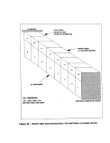 The time scales above offer a picture of the relative
importance of a given parameter or factor on mixing. For
example, the relatively short time scales for transport of bay
waters through tidal advection and residual advection
(gravitational), compared to the larger horizontal diffusion time
scale, support the notion that advection is the predominant
mixing process in Gastineau Channel in late summer. Also,
reduced vertical mixing would be expected in September due to a
stronger density gradient, resulting in a longer time scale for
vertical mixing.
3. Model Assumptions
The following is a list of major assumptions of this
modeling assessment:
1. Tidal flows decrease linearly in the up-channel
direction, based on continuity and the speed of the
tidal wave.
2. Tidal flows are uniformly distributed in the vertical
dimension.
3. Residual flows move up-channel at depth and down-
channel at the surface. There is no residual flow in
late winter.
4. Wastewater is trapped below 10 meters in summer and
reaches the surface in winter.
5. Wastewater is completely mixed in the first cell upon
discharge. Inflows to each cell are completely (and
instantaneously) mixed in both horizontal and vertical
dimensions.
6. Mixing beyond the Juneau-Douglas Bridge is not
significant. Freshwater inflows at the bridge boundary
are included.
7. Horizontal diffusion decreases from the mouth of the
channel (Stephens Passage) to the head (Juneau-Douglas
Bridge) in proportion to the square of the distance
from the mouth.
4. Solution Approach
The model was calibrated to salinity data observed in
September 1989 and March 1990 to represent stratified and non-
stratified conditions. Salinity levels were predicted using
estimates of seasonal flows to the system. Using fixed tidal and
residual advective flows, certain model parameters were adjusted
105
image:
The time scales above offer a picture of the relative
importance of a given parameter or factor on mixing. For
example, the relatively short time scales for transport of bay
waters through tidal advection and residual advection
(gravitational), compared to the larger horizontal diffusion time
scale, support the notion that advection is the predominant
mixing process in Gastineau Channel in late summer. Also,
reduced vertical mixing would be expected in September due to a
stronger density gradient, resulting in a longer time scale for
vertical mixing.
3. Model Assumptions
The following is a list of major assumptions of this
modeling assessment:
1. Tidal flows decrease linearly in the up-channel
direction, based on continuity and the speed of the
tidal wave.
2. Tidal flows are uniformly distributed in the vertical
dimension.
3. Residual flows move up-channel at depth and down-
channel at the surface. There is no residual flow in
late winter.
4. Wastewater is trapped below 10 meters in summer and
reaches the surface in winter.
5. Wastewater is completely mixed in the first cell upon
discharge. Inflows to each cell are completely (and
instantaneously) mixed in both horizontal and vertical
dimensions.
6. Mixing beyond the Juneau-Douglas Bridge is not
significant. Freshwater inflows at the bridge boundary
are included.
7. Horizontal diffusion decreases from the mouth of the
channel (Stephens Passage) to the head (Juneau-Douglas
Bridge) in proportion to the square of the distance
from the mouth.
4. Solution Approach
The model was calibrated to salinity data observed in
September 1989 and March 1990 to represent stratified and non-
stratified conditions. Salinity levels were predicted using
estimates of seasonal flows to the system. Using fixed tidal and
residual advective flows, certain model parameters were adjusted
105
image:
 to most closely., approximate actual salinity gradients by varying
(1) horizontal and vertical diffusion coefficients and (2)
residual current flows. Using the best-fit parameters derived
from the two calibrations, the model was then run with the
proposed discharge as an input. This method presumes that the
conditions of September 1989 and March 1990 are representative of
seasonal extremes (high and low runoff, respectively).
To the extent possible, available monitoring data from the
study area were used to estimate the important parameters
affecting mixing. Due to the limited data, the complexity of the
problem and number of variables involved, there is no single,
unique solution to the problem. The uncertainty in parameter
values necessitated using an approach of fixing parameters for
which data was available, and varying those for which limited
data was available until a reasonable solution was obtained.
Because tidal advection is included, a steady state solution
was not obtained. However, the model was run with a time step
and duration sufficient to obtain a dynamic, steady-state
solution. Time series plots are included in Appendix D7.
Finally, because WASP4 is a finite difference program used
for far-field analysis, it provides only average parameter values
for a given cell. Because of this, the values calculated by the
model do not represent local maxima within cells. This should be
considered in particular when reviewing the results for the cell
receiving the discharge loading, because local pollutant
concentrations around the discharge would be higher than the
average value calculated by this model.
5. Parameter Estimation
a. Characterization of Discharges
Echo Bay Alaska, Inc. originally proposed to discharge an
average of 49 cfs and maximum of 100 cfs of wastewater from the
tailings impoundment into Gastineau Channel near Thane (FEIS). A
subsequent analysis, which described the operating rule for
controlled effluent releases.from the impoundment, revised the
maximum flowrate to 200 cfs (SRK, April 1994), This operating
rule and the 30-year record of flows at the USGS station form the
basis for predicting daily outflows. Predictions of metals
concentrations in the discharge are described elsewhere in this
report (see Chapter VI).
The Gastineau Channel analysis is performed using fixed
discharge values designed to represent average and worst-case
conditions. The average condition is defined as the 95th
percentile value of running 180-day averages of the impoundment
loadings predicted in Chapter VI (Stage I of the project). The
180-day time frame was chosen on the basis of the approximate
106
image:
to most closely., approximate actual salinity gradients by varying
(1) horizontal and vertical diffusion coefficients and (2)
residual current flows. Using the best-fit parameters derived
from the two calibrations, the model was then run with the
proposed discharge as an input. This method presumes that the
conditions of September 1989 and March 1990 are representative of
seasonal extremes (high and low runoff, respectively).
To the extent possible, available monitoring data from the
study area were used to estimate the important parameters
affecting mixing. Due to the limited data, the complexity of the
problem and number of variables involved, there is no single,
unique solution to the problem. The uncertainty in parameter
values necessitated using an approach of fixing parameters for
which data was available, and varying those for which limited
data was available until a reasonable solution was obtained.
Because tidal advection is included, a steady state solution
was not obtained. However, the model was run with a time step
and duration sufficient to obtain a dynamic, steady-state
solution. Time series plots are included in Appendix D7.
Finally, because WASP4 is a finite difference program used
for far-field analysis, it provides only average parameter values
for a given cell. Because of this, the values calculated by the
model do not represent local maxima within cells. This should be
considered in particular when reviewing the results for the cell
receiving the discharge loading, because local pollutant
concentrations around the discharge would be higher than the
average value calculated by this model.
5. Parameter Estimation
a. Characterization of Discharges
Echo Bay Alaska, Inc. originally proposed to discharge an
average of 49 cfs and maximum of 100 cfs of wastewater from the
tailings impoundment into Gastineau Channel near Thane (FEIS). A
subsequent analysis, which described the operating rule for
controlled effluent releases.from the impoundment, revised the
maximum flowrate to 200 cfs (SRK, April 1994), This operating
rule and the 30-year record of flows at the USGS station form the
basis for predicting daily outflows. Predictions of metals
concentrations in the discharge are described elsewhere in this
report (see Chapter VI).
The Gastineau Channel analysis is performed using fixed
discharge values designed to represent average and worst-case
conditions. The average condition is defined as the 95th
percentile value of running 180-day averages of the impoundment
loadings predicted in Chapter VI (Stage I of the project). The
180-day time frame was chosen on the basis of the approximate
106
image:
 response time o.f the estuary to the pollutant discharge (see
Appendix D7). The worst-case condition assumes a continuous
discharge from the impoundment at maximum flow (200 cfs) and 95th
percentile maximum pollutant concentrations.
The AJ impoundment discharge is input to the model as a
loading (mass/time). Based on the predicted concentration of
each constituent above (for average and worst-case conditions)
and the average and maximum discharge flow rates, the following
total loadings (combined dissolved and particulate) in the
impoundment discharge are assumed.
Table 21: Impoundment Discharge Loading
Parameter
Mercury
Cyanide
Arsenic
Copper
Zinc
Lead
Avg
Discharge
(Ibs/day)
.079
138
2.9
76
155
59
Max
Discharge
(Ibs/day)
1.61
678
15.1
646
648
241
Initial dilution modeling by EPA (see Appendix D5) supports
predictions in the Comprehensive Report that the discharge plume
would be trapped beneath the surface by the density gradient
under stratified conditions. In the summer analysis, the entire
discharge loading was introduced to the bottom cell corresponding
to the proposed outfall location in Gastineau Channel.
Dilution modeling also indicates the potential for a
surfacing wastewater plume under unstratified conditions. In the
winter analysis, the discharge is uniformly distributed to the
bottom and top layer cells corresponding to the outfall location
to evaluate the impacts from a surfacing plume.
b. Mixing Dynamics - Salinity Calibration
The amount of mixing occurring in Gastineau Channel is a
function of processes driven by tides, freshwater discharges, and
wind In this analysis, the dynamics associated with the tide
and residual estuarine circulation were estimated by assuming
salinity is a conservative tracer. Wind was not incorporated
107
image:
response time o.f the estuary to the pollutant discharge (see
Appendix D7). The worst-case condition assumes a continuous
discharge from the impoundment at maximum flow (200 cfs) and 95th
percentile maximum pollutant concentrations.
The AJ impoundment discharge is input to the model as a
loading (mass/time). Based on the predicted concentration of
each constituent above (for average and worst-case conditions)
and the average and maximum discharge flow rates, the following
total loadings (combined dissolved and particulate) in the
impoundment discharge are assumed.
Table 21: Impoundment Discharge Loading
Parameter
Mercury
Cyanide
Arsenic
Copper
Zinc
Lead
Avg
Discharge
(Ibs/day)
.079
138
2.9
76
155
59
Max
Discharge
(Ibs/day)
1.61
678
15.1
646
648
241
Initial dilution modeling by EPA (see Appendix D5) supports
predictions in the Comprehensive Report that the discharge plume
would be trapped beneath the surface by the density gradient
under stratified conditions. In the summer analysis, the entire
discharge loading was introduced to the bottom cell corresponding
to the proposed outfall location in Gastineau Channel.
Dilution modeling also indicates the potential for a
surfacing wastewater plume under unstratified conditions. In the
winter analysis, the discharge is uniformly distributed to the
bottom and top layer cells corresponding to the outfall location
to evaluate the impacts from a surfacing plume.
b. Mixing Dynamics - Salinity Calibration
The amount of mixing occurring in Gastineau Channel is a
function of processes driven by tides, freshwater discharges, and
wind In this analysis, the dynamics associated with the tide
and residual estuarine circulation were estimated by assuming
salinity is a conservative tracer. Wind was not incorporated
107
image:
 into the quantitative analyis, though its influence on surface
flow is discussed qualitatively in this report.
c. Advection
WASP4 is capable of calculating the effects of both
advection and dispersion on water quality in the Channel. In the
absence of hydrodynamic model results, WASP4 accepts user-defined
flow fields and exchange fields. For this problem, several
advective flows are included. They include freshwater inflows,
residual flows, and tidal flows. Freshwater inflows and residual
flows were fixed, while a time varying function was used for
tidal flows. Figure 31 describes the advection routing
pictorially.
Average residual velocities from Figure 27 were coupled with
cell dimensions to obtain, the general range for residual flow at
the Stephens Passage boundary, with uniform vertical upwelling
from the lower layer assumed. The average residual velocity
(.005 m/sec) for the Thane current meter would suggest an average
inflow greater than 160 m3/sec -in the lower layer at the Stephens
Passage boundary. However, using the salt mass balance
methodology described by Pritchard (1955), the lower layer flow
for September 1989 is 27 m3/sec. The flowrate at the boundary
was adjusted in the salinity calibration. The best fit for
September 1989 salinity data was found at a residual flow of
approximately 60 m3/sec, within the range described above. The
residual flow for March (low stratification) was assumed to be
zero as a worst case assumption.
The tidal chart for August 29, 1990 (from Attachment 6 to
the Comprehensive Report) was input as a time variable flow
function which repeats itself each day until the model run is
complete.
The flows in the model correspond to current velocities that
are conservative in comparison to average conditions shown in the
current meter results for the 1990 and 1992 current meter
surveys. For example, the average tidal current at WASP4 station
#7 is approximately 1 cm/sec, while the corresponding average
current for station A in the 1990 current survey was
approximately 2 cm/sec.
d. Dispersion
Dispersion in estuaries also results from small-scale
turbulent diffusion and velocity shear. These factors result
from interactions within the tidal flow as well as between the
flow and the channel bottom. Velocity shear effects are created
by density structures due to freshwater inflow and also
interactions between tidal flows and the channel bottom.
108
image:
into the quantitative analyis, though its influence on surface
flow is discussed qualitatively in this report.
c. Advection
WASP4 is capable of calculating the effects of both
advection and dispersion on water quality in the Channel. In the
absence of hydrodynamic model results, WASP4 accepts user-defined
flow fields and exchange fields. For this problem, several
advective flows are included. They include freshwater inflows,
residual flows, and tidal flows. Freshwater inflows and residual
flows were fixed, while a time varying function was used for
tidal flows. Figure 31 describes the advection routing
pictorially.
Average residual velocities from Figure 27 were coupled with
cell dimensions to obtain, the general range for residual flow at
the Stephens Passage boundary, with uniform vertical upwelling
from the lower layer assumed. The average residual velocity
(.005 m/sec) for the Thane current meter would suggest an average
inflow greater than 160 m3/sec -in the lower layer at the Stephens
Passage boundary. However, using the salt mass balance
methodology described by Pritchard (1955), the lower layer flow
for September 1989 is 27 m3/sec. The flowrate at the boundary
was adjusted in the salinity calibration. The best fit for
September 1989 salinity data was found at a residual flow of
approximately 60 m3/sec, within the range described above. The
residual flow for March (low stratification) was assumed to be
zero as a worst case assumption.
The tidal chart for August 29, 1990 (from Attachment 6 to
the Comprehensive Report) was input as a time variable flow
function which repeats itself each day until the model run is
complete.
The flows in the model correspond to current velocities that
are conservative in comparison to average conditions shown in the
current meter results for the 1990 and 1992 current meter
surveys. For example, the average tidal current at WASP4 station
#7 is approximately 1 cm/sec, while the corresponding average
current for station A in the 1990 current survey was
approximately 2 cm/sec.
d. Dispersion
Dispersion in estuaries also results from small-scale
turbulent diffusion and velocity shear. These factors result
from interactions within the tidal flow as well as between the
flow and the channel bottom. Velocity shear effects are created
by density structures due to freshwater inflow and also
interactions between tidal flows and the channel bottom.
108
image:
 J-D BRIDGE
STEPHENS PASSAGE
1. TIDAL FLOOD
2. TIDAL EBB
3. RESIDUAL CIRCULATION (CONSTANT)
Arrow Length Represents Magnitude of Flow
ADVECTION ROUTING
Figure 31
image:
J-D BRIDGE
STEPHENS PASSAGE
1. TIDAL FLOOD
2. TIDAL EBB
3. RESIDUAL CIRCULATION (CONSTANT)
Arrow Length Represents Magnitude of Flow
ADVECTION ROUTING
Figure 31
image:
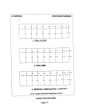 Turbulent .diffusion in the horizontal and vertical dimension
and velocity shear combine to cause dispersion of particles or
pollutant plumes. The mechanics describing the aggregate effect
are considered analogous to molecular diffusion; as a result, the
Fickian molecular diffusion equations are used to estimate
turbulent diffusion in a number of predictive tools, including
the WASP model framework. These estimates are driven by the
selection of horizontal dispersion coefficients and vertical
coefficients of eddy diffusivity.
No site-specific data are available to provide estimates of
the dispersion coefficient (K). Therefore, this parameter was
treated as a variable; coefficients were adjusted to fit the
salinity data. The horizontal dispersion coefficient was varied
as the square of the distance to the tidal source in accordance
with available literature (Bowden, 1967). The assumed increase
in horizontal dispersion down-channel is reasonable given the
proximity to Stephens Passage. The use of 0.16 m2/sec for the
uppermost cell, increasing to 10 m2/sec for the lowermost cell
obtained reasonable fits to the salinity data. Of note, this
order of magnitude of horizonta.1 dispersion resulted in model
results that matched the pattern shown by the aggregate salinity
data (higher salinity at station 12), whereas increasing the
values by one order of magnitude removed this pattern. The
chosen values fall within literature ranges for this parameter
(Kowalik, 1984).
Table 22: Horizontal Dispersion Coefficients
WASP Cells
1, 16
2, 15
3, 14
4, 13
5, 12
6, 11
7, 10
8, 9
Distance (m)
1725
3450
5175
6900
8625
10350
12075
13800
K (m2/sec)
.16
.60
1.4
. 2.5
3.9
5.6
7.6
10.0
For vertical coefficients of eddy diffusivity, no data are
available to provide estimates. Therefore, this parameter was
treated as a variable; it was adjusted to fit the salinity data
and account for relative stratification. The use of 0.00001
110
image:
Turbulent .diffusion in the horizontal and vertical dimension
and velocity shear combine to cause dispersion of particles or
pollutant plumes. The mechanics describing the aggregate effect
are considered analogous to molecular diffusion; as a result, the
Fickian molecular diffusion equations are used to estimate
turbulent diffusion in a number of predictive tools, including
the WASP model framework. These estimates are driven by the
selection of horizontal dispersion coefficients and vertical
coefficients of eddy diffusivity.
No site-specific data are available to provide estimates of
the dispersion coefficient (K). Therefore, this parameter was
treated as a variable; coefficients were adjusted to fit the
salinity data. The horizontal dispersion coefficient was varied
as the square of the distance to the tidal source in accordance
with available literature (Bowden, 1967). The assumed increase
in horizontal dispersion down-channel is reasonable given the
proximity to Stephens Passage. The use of 0.16 m2/sec for the
uppermost cell, increasing to 10 m2/sec for the lowermost cell
obtained reasonable fits to the salinity data. Of note, this
order of magnitude of horizonta.1 dispersion resulted in model
results that matched the pattern shown by the aggregate salinity
data (higher salinity at station 12), whereas increasing the
values by one order of magnitude removed this pattern. The
chosen values fall within literature ranges for this parameter
(Kowalik, 1984).
Table 22: Horizontal Dispersion Coefficients
WASP Cells
1, 16
2, 15
3, 14
4, 13
5, 12
6, 11
7, 10
8, 9
Distance (m)
1725
3450
5175
6900
8625
10350
12075
13800
K (m2/sec)
.16
.60
1.4
. 2.5
3.9
5.6
7.6
10.0
For vertical coefficients of eddy diffusivity, no data are
available to provide estimates. Therefore, this parameter was
treated as a variable; it was adjusted to fit the salinity data
and account for relative stratification. The use of 0.00001
110
image:
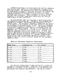 m2/sec for March and 0.00001 m2/sec for September obtained
relatively good fit solutions to the problem. The increased
diffusion in March is reasonable given the weak stratification at
that time, and both values fall within literature ranges for this
parameter (Kowalik, 1984).
e. Salinity Calibration
i; Freshwater Inflows
Freshwater flows into Gastineau Channel are important for
the salinity calibration. They were estimated using the values
from Echo Bay's "Gastineau Channel Freshwater Flushing Study"
(September 1991). In this report, flows were calculated for
individual .drainage basins based on discharge rates and relative
basin size for the creeks that have been gauged in the past (Gold
Creek 1918-1982, Lawson Creek 1970-1971, and Sheep Creek 1919-
1973) . Using the average Gold Creek flow for February 1990 and
September 1989 and the relative fraction of total flows for
August from the Flushing Study,, the flows for the other creeks
were estimated for February 1990 and September 1989.
Due to dimensional constraints of the WASP4 code, flows were
aggregated and introduced to cells in the model that correspond
to the largest creeks (cells 9 and 12) (See Figure 30).. For
predictive model runs, the flows into cell 12 associated with
Sheep Creek were reduced based on project predictions for flows
after dam construction.
ii. Ambient Salinity Data
As indicated in Figure 32, seawater monitoring stations
established by Echo Bay provide limited longitudinal coverage of
Gastineau Channel. To reduce potential for local influences to
mask salinity on a larger scale, Echo Bay stations were
aggregated for comparison with WASP4 predictions. Monitoring
stations were established in three areas of the channel: near
Stephens Passage, Thane, and Douglas. These locations correspond
to six WASP4 stations (one top layer and one bottom layer cell
for each location).
In order to translate salinity profiles into average cell
salinities for comparison to WASP4 predictions, weighted averages
were calculated for salinities measured from the surface to 10
meters, and from 10 meters to 35 meters (see Appendix Dl) .
iii Boundary Conditions - Salinity
Monitoring information for Stephens Passage and Taku Inlet
is not available for the time period of Gastineau Channel
monitoring (February 1990 and September 1989). In absence of
ill
image:
m2/sec for March and 0.00001 m2/sec for September obtained
relatively good fit solutions to the problem. The increased
diffusion in March is reasonable given the weak stratification at
that time, and both values fall within literature ranges for this
parameter (Kowalik, 1984).
e. Salinity Calibration
i; Freshwater Inflows
Freshwater flows into Gastineau Channel are important for
the salinity calibration. They were estimated using the values
from Echo Bay's "Gastineau Channel Freshwater Flushing Study"
(September 1991). In this report, flows were calculated for
individual .drainage basins based on discharge rates and relative
basin size for the creeks that have been gauged in the past (Gold
Creek 1918-1982, Lawson Creek 1970-1971, and Sheep Creek 1919-
1973) . Using the average Gold Creek flow for February 1990 and
September 1989 and the relative fraction of total flows for
August from the Flushing Study,, the flows for the other creeks
were estimated for February 1990 and September 1989.
Due to dimensional constraints of the WASP4 code, flows were
aggregated and introduced to cells in the model that correspond
to the largest creeks (cells 9 and 12) (See Figure 30).. For
predictive model runs, the flows into cell 12 associated with
Sheep Creek were reduced based on project predictions for flows
after dam construction.
ii. Ambient Salinity Data
As indicated in Figure 32, seawater monitoring stations
established by Echo Bay provide limited longitudinal coverage of
Gastineau Channel. To reduce potential for local influences to
mask salinity on a larger scale, Echo Bay stations were
aggregated for comparison with WASP4 predictions. Monitoring
stations were established in three areas of the channel: near
Stephens Passage, Thane, and Douglas. These locations correspond
to six WASP4 stations (one top layer and one bottom layer cell
for each location).
In order to translate salinity profiles into average cell
salinities for comparison to WASP4 predictions, weighted averages
were calculated for salinities measured from the surface to 10
meters, and from 10 meters to 35 meters (see Appendix Dl) .
iii Boundary Conditions - Salinity
Monitoring information for Stephens Passage and Taku Inlet
is not available for the time period of Gastineau Channel
monitoring (February 1990 and September 1989). In absence of
ill
image:
 data, EPA used .September 1988 information to establish boundary
values for the September 1989 calibration. For March 1990, the
longitudinal variation in salinity was minimal, and boundary
values for the surface layer were set approximately equal to the
those at the station nearest to Stephens Passage. Unfortunately,
the March 1990 sampling was conducted to depths greater than 15
meters; in this case, a value from the March 1992 Thane current
meter was used for lower layer salinity.
iv Salinity Simulation
A comparison of WASP4 predictions and seawater monitoring
data is depicted in Figure 33.
f. Boundary Conditions for Pollutants of Concern
Three boundaries were established in the model: one at the
mouth of the bay, and one at the entrance of Gold Creek and Sheep
Creek. It is assumed that no mixing occurs beyond the Juneau-
Douglas Bridge, though inflow from Gold Creek and Salmon Creek is
included.
EPA reviewed 1990 seawater monitoring data collected by Echo
Bay in Gastineau Channel to establish boundary conditions for the
model. Gastineau Channel values are used as boundary values at
the entrance to Stephens Passage and creek inflows. Mean values
(excluding non-detects) are used in the model. All data are
drawn from the Comprehensive Report (Document #2; EBA, 1992).
The table below summarizes the values used in the model (all
metals values are in "total recoverable").
Table 23: Gastineau Channel Background Water Quality
Parameter
Mercury
Cyanide
Arsenic
Copper
Zinc
Lead
Cone, (ug/1)
.009
NA(0)
1.4
0.8
2.3
0.2
112
image:
data, EPA used .September 1988 information to establish boundary
values for the September 1989 calibration. For March 1990, the
longitudinal variation in salinity was minimal, and boundary
values for the surface layer were set approximately equal to the
those at the station nearest to Stephens Passage. Unfortunately,
the March 1990 sampling was conducted to depths greater than 15
meters; in this case, a value from the March 1992 Thane current
meter was used for lower layer salinity.
iv Salinity Simulation
A comparison of WASP4 predictions and seawater monitoring
data is depicted in Figure 33.
f. Boundary Conditions for Pollutants of Concern
Three boundaries were established in the model: one at the
mouth of the bay, and one at the entrance of Gold Creek and Sheep
Creek. It is assumed that no mixing occurs beyond the Juneau-
Douglas Bridge, though inflow from Gold Creek and Salmon Creek is
included.
EPA reviewed 1990 seawater monitoring data collected by Echo
Bay in Gastineau Channel to establish boundary conditions for the
model. Gastineau Channel values are used as boundary values at
the entrance to Stephens Passage and creek inflows. Mean values
(excluding non-detects) are used in the model. All data are
drawn from the Comprehensive Report (Document #2; EBA, 1992).
The table below summarizes the values used in the model (all
metals values are in "total recoverable").
Table 23: Gastineau Channel Background Water Quality
Parameter
Mercury
Cyanide
Arsenic
Copper
Zinc
Lead
Cone, (ug/1)
.009
NA(0)
1.4
0.8
2.3
0.2
112
image:
 134"25'
134°20'
134°15'
134° 10'
58° 15'
58° 10'
134°05'
DOUGLAS
•
ISLAND
MAINLAND
V.
. .
o~
2
W
• i
••
V
Figure 32 : Salinity Stations In Relation to WASP4 Grid
image:
134"25'
134°20'
134°15'
134° 10'
58° 15'
58° 10'
134°05'
DOUGLAS
•
ISLAND
MAINLAND
V.
. .
o~
2
W
• i
••
V
Figure 32 : Salinity Stations In Relation to WASP4 Grid
image:
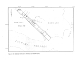 Comparison of Actual vs. Predicted Salinities
September 1989
Top
Actual I
I Top
I Predicted
Bottom
Actual
Salinity in ppt
35
Bottom
Predicted
Stephens "hane Douglas
Comparison of Actual vs. Predicted Salinities
March 1990
I Top
Actual
Top
Predicted
Bottom
Actual
Salinity in ppt
35
Bottom
Predicted
Stephens Thane Douglas
Figure 33 : Salinity Calibration Results
image:
Comparison of Actual vs. Predicted Salinities
September 1989
Top
Actual I
I Top
I Predicted
Bottom
Actual
Salinity in ppt
35
Bottom
Predicted
Stephens "hane Douglas
Comparison of Actual vs. Predicted Salinities
March 1990
I Top
Actual
Top
Predicted
Bottom
Actual
Salinity in ppt
35
Bottom
Predicted
Stephens Thane Douglas
Figure 33 : Salinity Calibration Results
image:
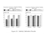 6. Projected Impacts
a. Applicable Water Quality Standards
The state of Alaska water quality standards are codified in
18 AAC 70. The regulation establishes beneficial uses of Alaskan
waters as well as the water quality criteria that must be met to
assure protection of a given use.
b. Beneficial Uses Affected
Gastineau Channel is protected under the Alaska Water
Quality Standards for the following beneficial uses:
• Water supply for aquaculture, seafood processing, and
industrial uses.
• Contact and secondary recreation.
• Growth and propagation of fish, shellfish, other
aquatic life, and wildlife.
• Harvesting for consumption of raw mollusks or other raw
aquatic life.
c. Water Quality Criteria
The State of Alaska water quality standards establish the
following criteria for total recoverable metals and cyanide in
marine waters, designed to protect against chronic toxicity to
aquatic organisms (for arsenic only, the limiting criterion is
for protection against human health effects from fish ingestion) :
Table 24: Water Quality criteria
Parameter
Mercury
Cyanide
Arsenic
Copper
Lead
Zinc
Applicable
Criterion
(ug/1)
.025
1.0
1.4
2.9
8.5
86.0
115
image:
6. Projected Impacts
a. Applicable Water Quality Standards
The state of Alaska water quality standards are codified in
18 AAC 70. The regulation establishes beneficial uses of Alaskan
waters as well as the water quality criteria that must be met to
assure protection of a given use.
b. Beneficial Uses Affected
Gastineau Channel is protected under the Alaska Water
Quality Standards for the following beneficial uses:
• Water supply for aquaculture, seafood processing, and
industrial uses.
• Contact and secondary recreation.
• Growth and propagation of fish, shellfish, other
aquatic life, and wildlife.
• Harvesting for consumption of raw mollusks or other raw
aquatic life.
c. Water Quality Criteria
The State of Alaska water quality standards establish the
following criteria for total recoverable metals and cyanide in
marine waters, designed to protect against chronic toxicity to
aquatic organisms (for arsenic only, the limiting criterion is
for protection against human health effects from fish ingestion) :
Table 24: Water Quality criteria
Parameter
Mercury
Cyanide
Arsenic
Copper
Lead
Zinc
Applicable
Criterion
(ug/1)
.025
1.0
1.4
2.9
8.5
86.0
115
image:
 d. Model: Predictions
Figures 34 through 36 depict comparisons of the water
quality standard concentration and the predicted average and
maximum pollutant concentrations from the WASP4 model analysis.
For each case (top/bottom layer, summer/winter), predictions for
the entire channel length are shown, with the Juneau-Douglas
bridge at the left of each graph and the entrance to Stephens
Passage at the right. Results in tabular form are included in
Appendix D8.
For the winter case, one set of plots represents
concentrations in both the top and bottom layer. This is because
concentrations in the two layers are approximately equal for the
winter case, due to the assumption that a surfacing discharge
plume would be uniformly distributed in the water column during
the winter.
7. Conclusions
The analysis above indicat.es that far-field mixing in
Gastineau Channel is significantly limited for discharges of the
magnitude proposed for the AJ impoundment. As a result, impacts
from the impoundment discharge are predicted to occur on a
channel-wide scale. This contradicts the conclusion in the
Comprehensive Report (EBA, 1992) that sufficient dilution of the
proposed discharge would be achieved in a confined mixing zone
around the diffuser.
Based on the model assumptions described herein, the
predicted average discharges from the AJ Mine are projected to
violate the Alaska water quality standards for arsenic, copper,
and cyanide in Gastineau Channel on a channel-wide scale. Under
worst-case assumptions, mercury and lead standards would be
violated as well.
8. Uncerta inty
a. Wind
Wind-driven circulation is not considered in this
assessment, though it is acknowledged as one of the important
factors affecting circulation. Southeast winds would serve to
counter the flushing mechanisms due to tidal and gravitational
advection, generally restricting or reversing the migration of
surface waters out of the channel and reducing the dilution of
pollutants. Local, episodic impacts to surface waters,
particularly with a surfacing plume, are not addressed by this
report.
lie
image:
d. Model: Predictions
Figures 34 through 36 depict comparisons of the water
quality standard concentration and the predicted average and
maximum pollutant concentrations from the WASP4 model analysis.
For each case (top/bottom layer, summer/winter), predictions for
the entire channel length are shown, with the Juneau-Douglas
bridge at the left of each graph and the entrance to Stephens
Passage at the right. Results in tabular form are included in
Appendix D8.
For the winter case, one set of plots represents
concentrations in both the top and bottom layer. This is because
concentrations in the two layers are approximately equal for the
winter case, due to the assumption that a surfacing discharge
plume would be uniformly distributed in the water column during
the winter.
7. Conclusions
The analysis above indicat.es that far-field mixing in
Gastineau Channel is significantly limited for discharges of the
magnitude proposed for the AJ impoundment. As a result, impacts
from the impoundment discharge are predicted to occur on a
channel-wide scale. This contradicts the conclusion in the
Comprehensive Report (EBA, 1992) that sufficient dilution of the
proposed discharge would be achieved in a confined mixing zone
around the diffuser.
Based on the model assumptions described herein, the
predicted average discharges from the AJ Mine are projected to
violate the Alaska water quality standards for arsenic, copper,
and cyanide in Gastineau Channel on a channel-wide scale. Under
worst-case assumptions, mercury and lead standards would be
violated as well.
8. Uncerta inty
a. Wind
Wind-driven circulation is not considered in this
assessment, though it is acknowledged as one of the important
factors affecting circulation. Southeast winds would serve to
counter the flushing mechanisms due to tidal and gravitational
advection, generally restricting or reversing the migration of
surface waters out of the channel and reducing the dilution of
pollutants. Local, episodic impacts to surface waters,
particularly with a surfacing plume, are not addressed by this
report.
lie
image:
 Figure 34
WASP Model Results - Summer
Bottom Layer
(solid dot = max, clear dot = avg, square = standard)
Arsenic
Copper
o
3
2.2
2
1.8
1.6
1.4
1.2
0 4,000 8,000 12,000
2,000 6,000 10,000 14,000
Dist. from J-D Bridge (m)
0 4,000 8,000 12,000
2,000 6,000 10,000 14,000
Distance from J-D Bridge (m)
50
20 -
10 -
5
2
0.5
0.2
Cyanide
•—•—•-
0.1
0.05 •
0.03
3 0.02
0.01
0 4,000 8,000 12,000
2,000 6,000 10,000 14,000
Distance from J-D Bridge (m)
0.005
Mercury
\
0 4,000 8,000 12,000
2,000 6,000 10,000 14,000
Distance from J-D Bridge (m)
image:
Figure 34
WASP Model Results - Summer
Bottom Layer
(solid dot = max, clear dot = avg, square = standard)
Arsenic
Copper
o
3
2.2
2
1.8
1.6
1.4
1.2
0 4,000 8,000 12,000
2,000 6,000 10,000 14,000
Dist. from J-D Bridge (m)
0 4,000 8,000 12,000
2,000 6,000 10,000 14,000
Distance from J-D Bridge (m)
50
20 -
10 -
5
2
0.5
0.2
Cyanide
•—•—•-
0.1
0.05 •
0.03
3 0.02
0.01
0 4,000 8,000 12,000
2,000 6,000 10,000 14,000
Distance from J-D Bridge (m)
0.005
Mercury
\
0 4,000 8,000 12,000
2,000 6,000 10,000 14,000
Distance from J-D Bridge (m)
image:
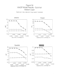 WASP Model Results - Summer
Bottom Layer
(solid dot = max, clear dot = avg, square = standard)
Lead
Zinc
14
12
10
- 8
o
6
4
2
200
100
50
> 20
10
5
0 4,000 8,000 12,000
2,000 6,000 10,000 14,000
Dist. from J-D Bridge (m)
0 4,000 8,000 12,000
2,000 6,000 10,000 14,000
Distance from J-D Bridge (m)
image:
WASP Model Results - Summer
Bottom Layer
(solid dot = max, clear dot = avg, square = standard)
Lead
Zinc
14
12
10
- 8
o
6
4
2
200
100
50
> 20
10
5
0 4,000 8,000 12,000
2,000 6,000 10,000 14,000
Dist. from J-D Bridge (m)
0 4,000 8,000 12,000
2,000 6,000 10,000 14,000
Distance from J-D Bridge (m)
image:
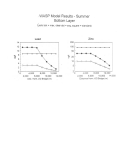 Figure 35
WASP Model Results - Summer
Top Layer
(solid dot = max, clear dot = avg, square = standard)
Arsenic
Copper
1.9
1.8
1.7
1.6
1.5
1.4
1.3
0 4,000 8,000 12,000
2,000 6,000 10,000 14,000
Dist. from J-D Bridge (m)
30
20
10
' 5
2
:
1
0 4,000 8,000 12,000
2,000 6,000 10,000 14,000
Distance from J-D Bridge (m)
Cyanide
Mercury
50
20
10
5
1
0.5
=
2~000 6,000 10,000 14,000
4,000 8,000 12,000
Distance from J-D Bridge (m)
0.1
0.05
0.03
0.02
0.01
0.005
\
0 4,000 8,000 12,000
2,000 6,000 10,000 14,000
Distance from J-D Bridge (m)
image:
Figure 35
WASP Model Results - Summer
Top Layer
(solid dot = max, clear dot = avg, square = standard)
Arsenic
Copper
1.9
1.8
1.7
1.6
1.5
1.4
1.3
0 4,000 8,000 12,000
2,000 6,000 10,000 14,000
Dist. from J-D Bridge (m)
30
20
10
' 5
2
:
1
0 4,000 8,000 12,000
2,000 6,000 10,000 14,000
Distance from J-D Bridge (m)
Cyanide
Mercury
50
20
10
5
1
0.5
=
2~000 6,000 10,000 14,000
4,000 8,000 12,000
Distance from J-D Bridge (m)
0.1
0.05
0.03
0.02
0.01
0.005
\
0 4,000 8,000 12,000
2,000 6,000 10,000 14,000
Distance from J-D Bridge (m)
image:
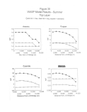 WASP Model Results - Summer
Top Layer
(solid dot = max, clear dot = avg, square = standard)
Lead
Zinc
10
s
6
4
2
200
100
50
§> 20
1C
5
0 4,000 8,000 12,000
2,000 6,000 10,000 14,000
Dist. from J-D Bridge (m)
0 4,000 8,000 12,000
2,000 6,000 10,000 14,000
Distance from J-D Bridge (m)
image:
WASP Model Results - Summer
Top Layer
(solid dot = max, clear dot = avg, square = standard)
Lead
Zinc
10
s
6
4
2
200
100
50
§> 20
1C
5
0 4,000 8,000 12,000
2,000 6,000 10,000 14,000
Dist. from J-D Bridge (m)
0 4,000 8,000 12,000
2,000 6,000 10,000 14,000
Distance from J-D Bridge (m)
image:
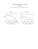 Figure 36
WASP Mode! Results - Winter
Top and Bottom Layer
(solid dot = max, clear dot = avg, square = standard)
Arsenic
0 4,000 8,000 12,000
2,000 6,000 10,000 14,000
Dist. from J-D Bridge (m)
50
en
a
30 -
20 -
10
5
2
i
Copper
• • • *.
0 4,000 8,000 12,000
2,000 6,000 - 10,000 14,000
Distance from J-D Bridge (m)
Cyanide
0.1
0.05 p-
0.03
0.02
0.01
0.005
4,000 8,000 12,000
2,000 6,000 10,000 14,000
Distance from J-D Bridge (m)
Mercury
\
4,000 8,000 12,000
2,000 ' 6,000 10,000 14,000
Distance from J-D Bridge (m)
image:
Figure 36
WASP Mode! Results - Winter
Top and Bottom Layer
(solid dot = max, clear dot = avg, square = standard)
Arsenic
0 4,000 8,000 12,000
2,000 6,000 10,000 14,000
Dist. from J-D Bridge (m)
50
en
a
30 -
20 -
10
5
2
i
Copper
• • • *.
0 4,000 8,000 12,000
2,000 6,000 - 10,000 14,000
Distance from J-D Bridge (m)
Cyanide
0.1
0.05 p-
0.03
0.02
0.01
0.005
4,000 8,000 12,000
2,000 6,000 10,000 14,000
Distance from J-D Bridge (m)
Mercury
\
4,000 8,000 12,000
2,000 ' 6,000 10,000 14,000
Distance from J-D Bridge (m)
image:
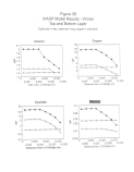 WASP Model Results - Winter
Top and Bottom Layer
(solid dot = max, clear dot = avg, square = standard)
Lead
Zinc
f
12
10
8
6
4
2
0
G-
200
100
50
» 20
10
0 4,000 8,000 12,000
2,000 6,000 10,000 14,000
Dist. from J-D Bridge (m)
F G-
0 4,000 8,000 12,000
2,000 6,000 10,000 14,000
Distance from J-D Bridge (m)
image:
WASP Model Results - Winter
Top and Bottom Layer
(solid dot = max, clear dot = avg, square = standard)
Lead
Zinc
f
12
10
8
6
4
2
0
G-
200
100
50
» 20
10
0 4,000 8,000 12,000
2,000 6,000 10,000 14,000
Dist. from J-D Bridge (m)
F G-
0 4,000 8,000 12,000
2,000 6,000 10,000 14,000
Distance from J-D Bridge (m)
image:
 b. Local Effects
This assessment provides only average pollutant
concentrations for a given cell. Because of this, the values
calculated by the model do not represent local maxima within
cells. This should be considered in reviewing the results for
the cell receiving the discharge loading, because local pollutant
concentrations around the discharge would be higher than the
average value calculated by this model.
c. Discharge Quality
Because this report relies on the.impoundment assessment for
estimates of the quality of the discharge, the predictions and
conclusions herein carried forward the uncertainties associated
with those estimates.
d. Discharge Quantity
As stated earlier in the r-eport, the quantity of the
discharge is somewhat uncertain. A significant change (from 100
to 200 cfs) has been made to maximum flow volume estimates in the
period since the EIS was finalized. This was due in part to
changes in project designs and flow routing. Because of the
importance to loadings from the discharge, this indicates the
potential for inaccuracies in any predictions of impacts to
Gastineau Channel from this'proposed facility.
e. Potential Impacts Beyond the Juneau Douglas Bridge
As stated earlier in the chapter, the drift card studies
have indicated the potential for surface waters and pollutants to
migrate beyond the Juneau-Douglas bridge and reach the tide flats
around the Mendenhall River and Fitz Cove. This highlights the
potential for impacts beyond the boundaries of the modeled
system. Persistent southeast winds and a surfacing plume
(winter) could restrict flushing in the surface and impact these
locations above the bridge.
123
image:
b. Local Effects
This assessment provides only average pollutant
concentrations for a given cell. Because of this, the values
calculated by the model do not represent local maxima within
cells. This should be considered in reviewing the results for
the cell receiving the discharge loading, because local pollutant
concentrations around the discharge would be higher than the
average value calculated by this model.
c. Discharge Quality
Because this report relies on the.impoundment assessment for
estimates of the quality of the discharge, the predictions and
conclusions herein carried forward the uncertainties associated
with those estimates.
d. Discharge Quantity
As stated earlier in the r-eport, the quantity of the
discharge is somewhat uncertain. A significant change (from 100
to 200 cfs) has been made to maximum flow volume estimates in the
period since the EIS was finalized. This was due in part to
changes in project designs and flow routing. Because of the
importance to loadings from the discharge, this indicates the
potential for inaccuracies in any predictions of impacts to
Gastineau Channel from this'proposed facility.
e. Potential Impacts Beyond the Juneau Douglas Bridge
As stated earlier in the chapter, the drift card studies
have indicated the potential for surface waters and pollutants to
migrate beyond the Juneau-Douglas bridge and reach the tide flats
around the Mendenhall River and Fitz Cove. This highlights the
potential for impacts beyond the boundaries of the modeled
system. Persistent southeast winds and a surfacing plume
(winter) could restrict flushing in the surface and impact these
locations above the bridge.
123
image:
 VIII. RISK .pF LONG-TERM CONTAMINATION
A. Introduction
The goal of this analysis is to determine the likelihood
that a healthy aquatic food chain and habitat system would
develop and persist after the cessation of mining and the active
use of the impoundment for tailings disposal. The physical and
chemical characteristics of the impoundment and surrounding area
would dictate the expected food chain and habitats.
The majority of the chemical impact analysis is contained in
an ecological risk analysis presented later in this chapter. It
is based on modeling of predicted residual chemical levels in the
impoundment. A review of relevant literature on subaqueous
disposal of mine tailings is included as well. This is followed
by an assessment of the potential for the tailings to generate
acid and mobilize metals in the tailings.
The following is a description of impoundment geomorphology,
and its setting from the watershed and physical standpoint. This
analysis will be carried through to discuss the expected
biological community that would be expected to develop in the
impoundment in the absence of any chemical contamination.
B. Watershed/Phvs ica1 Setting
Following closure of the AJ Mine, the resulting tailings
impoundment would rest in a typical U-shaped glacial valley with
steep side slopes. Elevation would be approximately 932' MLLW.
The long narrow body of water would be 20 feet deep at a minimum,
and 2.5 miles long, with a surface area of 420 acres (FEIS p. 4-
20). When there is a weakly developed thermocline (late summer),
the impoundment would have an approximate surface temperature of
11 degrees Celsius and a bottom temperature of 7 degrees Celsius,
otherwise the impoundment would be relatively isothermal (HDR,
1990). The impoundment would generally freeze from November
through March.
Due to the steep valley walls, the impoundment would be
avalanche prone. The applicant proposes to construct flat bench
areas out of waste rock from the mine. The benches would be
constructed along the impoundment shoreline in- avalanche chute
areas for avalanche dissipation (BLM, 1992). Following mine
closure, the shoreline sites would be recontoured to provide
relatively flat beach areas (BLM, 1992).
ADFG has required as mitigation diversion of an average
annual flow of 16.3 cfs from the upper watershed to Sheep Creek
below the impoundment dam and above the hatchery. This would
require diversion structures at the inlet creeks above the
impoundment, and changes in water flows and other inputs (e.g.,
124
image:
VIII. RISK .pF LONG-TERM CONTAMINATION
A. Introduction
The goal of this analysis is to determine the likelihood
that a healthy aquatic food chain and habitat system would
develop and persist after the cessation of mining and the active
use of the impoundment for tailings disposal. The physical and
chemical characteristics of the impoundment and surrounding area
would dictate the expected food chain and habitats.
The majority of the chemical impact analysis is contained in
an ecological risk analysis presented later in this chapter. It
is based on modeling of predicted residual chemical levels in the
impoundment. A review of relevant literature on subaqueous
disposal of mine tailings is included as well. This is followed
by an assessment of the potential for the tailings to generate
acid and mobilize metals in the tailings.
The following is a description of impoundment geomorphology,
and its setting from the watershed and physical standpoint. This
analysis will be carried through to discuss the expected
biological community that would be expected to develop in the
impoundment in the absence of any chemical contamination.
B. Watershed/Phvs ica1 Setting
Following closure of the AJ Mine, the resulting tailings
impoundment would rest in a typical U-shaped glacial valley with
steep side slopes. Elevation would be approximately 932' MLLW.
The long narrow body of water would be 20 feet deep at a minimum,
and 2.5 miles long, with a surface area of 420 acres (FEIS p. 4-
20). When there is a weakly developed thermocline (late summer),
the impoundment would have an approximate surface temperature of
11 degrees Celsius and a bottom temperature of 7 degrees Celsius,
otherwise the impoundment would be relatively isothermal (HDR,
1990). The impoundment would generally freeze from November
through March.
Due to the steep valley walls, the impoundment would be
avalanche prone. The applicant proposes to construct flat bench
areas out of waste rock from the mine. The benches would be
constructed along the impoundment shoreline in- avalanche chute
areas for avalanche dissipation (BLM, 1992). Following mine
closure, the shoreline sites would be recontoured to provide
relatively flat beach areas (BLM, 1992).
ADFG has required as mitigation diversion of an average
annual flow of 16.3 cfs from the upper watershed to Sheep Creek
below the impoundment dam and above the hatchery. This would
require diversion structures at the inlet creeks above the
impoundment, and changes in water flows and other inputs (e.g.,
124
image:
 sediments) from the upper watershed to the impoundment (Letter
from ADFG, Lana Shea to Frank Bergstrom dated February 2, 1994).
Average annual discharge from the Sheep Creek watershed
above the proposed dam is 49 cfs. During mine operation 16 cfs
would be diverted, via upstream diversion structures, around the
impoundment to lower Sheep Creek. Monthly stream flows from the
watershed vary seasonally from lows of 6 cfs in February up to
nearly 100 cfs in June (see Table 2). Residence time in the
impoundment (the amount of time it takes for a particle of water
to enter and then leave the impoundment) is calculated to be 4
months in the summer and 7.2 months in February (p. H-8) .
Natural sediment loading into the impoundment would be low, with
total annual sediment transport into the impoundment of 1200
cubic yards (p. 4-89). The addition of upstream diversion
structures would decrease sediment transport.
Following use as a tailings treatment facility, the bottom
of the impoundment would be covered with well-graded silty-sand
tailings. These tailings could be periodically resuspended by
large avalanche events. At a minimum, 20 feet of water would
cover mine tailings. It is planned that water level variations
should result only in increased depth and not decreased depth
over the tailings.
C. Uncertainty Factors
The above description includes information that is
relatively certain from the project's supporting documentation.
However, the following are some important dynamic "unknowns" that
could have a large impact on the resulting biological community.
Resuspension of sediments by Taku winds (FEIS Vl-3-2: fastest
one-minute wind Nov 68 = 58 mph) could have an impact on the
impoundment's biological community, including smothering,
toxicity, and turbidity.
Avalanches would also play a role in resuspension within the
impoundment, depending on the season, and in the development of
vegetation on the avalanche dissipators.
Water level fluctuations in the impoundment would affect
riparian and nearshore vegetation, depending on the degree and
frequency of inundation. Water level fluctuation extremes are a
relative unknown though theoretically the impoundment level can
be managed as desired by the resource agencies. Reservoirs whose
surface level fluctuates according to unnatural cycles generally
result in stressed communities of macrophytes in the zone that is
repeatedly inundated and then dewatered, especially if this
occurs during the growing season.
In addition, the impoundment as proposed to date is an
unusual feature in southeast Alaska. A steep-sided fjord-like
125
image:
sediments) from the upper watershed to the impoundment (Letter
from ADFG, Lana Shea to Frank Bergstrom dated February 2, 1994).
Average annual discharge from the Sheep Creek watershed
above the proposed dam is 49 cfs. During mine operation 16 cfs
would be diverted, via upstream diversion structures, around the
impoundment to lower Sheep Creek. Monthly stream flows from the
watershed vary seasonally from lows of 6 cfs in February up to
nearly 100 cfs in June (see Table 2). Residence time in the
impoundment (the amount of time it takes for a particle of water
to enter and then leave the impoundment) is calculated to be 4
months in the summer and 7.2 months in February (p. H-8) .
Natural sediment loading into the impoundment would be low, with
total annual sediment transport into the impoundment of 1200
cubic yards (p. 4-89). The addition of upstream diversion
structures would decrease sediment transport.
Following use as a tailings treatment facility, the bottom
of the impoundment would be covered with well-graded silty-sand
tailings. These tailings could be periodically resuspended by
large avalanche events. At a minimum, 20 feet of water would
cover mine tailings. It is planned that water level variations
should result only in increased depth and not decreased depth
over the tailings.
C. Uncertainty Factors
The above description includes information that is
relatively certain from the project's supporting documentation.
However, the following are some important dynamic "unknowns" that
could have a large impact on the resulting biological community.
Resuspension of sediments by Taku winds (FEIS Vl-3-2: fastest
one-minute wind Nov 68 = 58 mph) could have an impact on the
impoundment's biological community, including smothering,
toxicity, and turbidity.
Avalanches would also play a role in resuspension within the
impoundment, depending on the season, and in the development of
vegetation on the avalanche dissipators.
Water level fluctuations in the impoundment would affect
riparian and nearshore vegetation, depending on the degree and
frequency of inundation. Water level fluctuation extremes are a
relative unknown though theoretically the impoundment level can
be managed as desired by the resource agencies. Reservoirs whose
surface level fluctuates according to unnatural cycles generally
result in stressed communities of macrophytes in the zone that is
repeatedly inundated and then dewatered, especially if this
occurs during the growing season.
In addition, the impoundment as proposed to date is an
unusual feature in southeast Alaska. A steep-sided fjord-like
125
image:
 impoundment with relatively shallow water depth is not frequently
found in this landscape. A query to Alaska Fish and Game
discovered no representative natural lake from which to base
predictions of biological activity for the proposed design
(Letter Dr. Dana Schmidt, Alaska Fish and Game to Justine Barton,
dated 12/ 13/93).
D.. Predicted Community Components.
1. Benthos
With a sedimentation rate of only 1200 cubic yards/year,
impoundment tailings coverage and natural substrate for benthos
is not expected in the short term. The coarseness of the
tailings as well as chemical inputs would play an important role
in determining whether a benthic community could establish on the
tailings themselves. No analysis to date has focussed on the
grain size requirements of a healthy benthic community in this
environment. Additionally the impoundment lacks a food web base
due to expected low input of organic material, and lacks an
existing lake benthic community, to serve as a source for
recruitment to the impoundment.
2. Plankton
An analysis of anticipated phytoplankton and zooplankton
populations is required, especially considering the lake's
shallowness and planktonic migrations based on depth. It is
highly unlikely that mining discharges will increase the
productivity of the impoundment compared to a similar impoundment
with no discharges of tailings. An analysis of nutrients and
their anticipated concentrations in the tailings pond water is
needed, including an analysis of any break down products.
(Enclosure A from Letter Lana C. Shea, Alaska Fish and Game to
Bill Riley, dated 1/10/94).
3... Fish
Fish populations are not anticipated in the impoundment
during mine operation. Subsequent to mine closure, fish
populations are unlikely without a managed food base. Insect
production and transport by the inflowing small streams will not
provide enough food to sustain fish, and the diversion dams will
exacerbate this. In addition, the impoundment lacks the habitat
characteristics required for potential species survival (e.g.
cover, spawning areas). The habitat constructed for fish would
depend on the species desired and whether the impoundment is to
be managed for fish, based on anticipated chemical levels in
tissues (e.g. kokanee, cutthroat). As stated by ADFG (1/10/94
ltr-pA3) "We do not know if the stream resident char currently
found in upper Sheep Creek could adapt and survive in the
proposed tailings pond (independent of toxicity issues)», and it
126
image:
impoundment with relatively shallow water depth is not frequently
found in this landscape. A query to Alaska Fish and Game
discovered no representative natural lake from which to base
predictions of biological activity for the proposed design
(Letter Dr. Dana Schmidt, Alaska Fish and Game to Justine Barton,
dated 12/ 13/93).
D.. Predicted Community Components.
1. Benthos
With a sedimentation rate of only 1200 cubic yards/year,
impoundment tailings coverage and natural substrate for benthos
is not expected in the short term. The coarseness of the
tailings as well as chemical inputs would play an important role
in determining whether a benthic community could establish on the
tailings themselves. No analysis to date has focussed on the
grain size requirements of a healthy benthic community in this
environment. Additionally the impoundment lacks a food web base
due to expected low input of organic material, and lacks an
existing lake benthic community, to serve as a source for
recruitment to the impoundment.
2. Plankton
An analysis of anticipated phytoplankton and zooplankton
populations is required, especially considering the lake's
shallowness and planktonic migrations based on depth. It is
highly unlikely that mining discharges will increase the
productivity of the impoundment compared to a similar impoundment
with no discharges of tailings. An analysis of nutrients and
their anticipated concentrations in the tailings pond water is
needed, including an analysis of any break down products.
(Enclosure A from Letter Lana C. Shea, Alaska Fish and Game to
Bill Riley, dated 1/10/94).
3... Fish
Fish populations are not anticipated in the impoundment
during mine operation. Subsequent to mine closure, fish
populations are unlikely without a managed food base. Insect
production and transport by the inflowing small streams will not
provide enough food to sustain fish, and the diversion dams will
exacerbate this. In addition, the impoundment lacks the habitat
characteristics required for potential species survival (e.g.
cover, spawning areas). The habitat constructed for fish would
depend on the species desired and whether the impoundment is to
be managed for fish, based on anticipated chemical levels in
tissues (e.g. kokanee, cutthroat). As stated by ADFG (1/10/94
ltr-pA3) "We do not know if the stream resident char currently
found in upper Sheep Creek could adapt and survive in the
proposed tailings pond (independent of toxicity issues)», and it
126
image:
 is not clear how robust the resulting population might be" since
they require spawning habitat and suitable aquatic insect fauna.
4. Macrophvtes
The Mine Environment Neutral Drainage (MEND) studies,
conducted by a consortium of Canadian government agencies and
industry representatives, examined lakes in Canada that have been
used in the past for subaqueous disposal of mine tailings. Four
potentially relevant Canadian lakes studied included Buttle Lake,
Anderson Lake, Mandy Lake and Benson Lake. The MEND case studies
at Mandy and Benson lakes show that macrophytes can take up
metals when grown directly on tailings.
The argument for subaqueous disposal is that all tailings
will be covered by water such that no contact with rooted
macrophytes is likely. However, the potential magnitide of
resuspension events (e.g. Taku winds, avalanches) and
resuspension of tailings into shallow areas limits the analysis
of expected species. This is especially of concern on the
littoral and fringe zones of the impoundment where dabbling
waterfowl and macrophytes are anticipated, and where other routes
of exposure to the tailings besides consumption of leafy portions
of the macrophytes (e.g. sediment, roots) could be a factor.
5_:_ Littoral /Riparian (fringe) zone and Vegetation
The post-closure vegetation expected on the surrounding
slopes and avalanche dissipators is likely to be alder and
shrubby vegetation. It has been suggested that the impoundment's
shoreline would create new wetland habitats, however, this has
not been analyzed, and based on steep surrounding terrain seems
unlikely. Obviously any shoreline vegetation would be greatly
influenced by the impoundment's operation with respect to how the
surface water level fluctuates. Any vegetation growing on the
avalanche dissipators would be affected by avalanche events.
6j. Wildlife
It is likely that the tailings impoundment will be
attractive to birds, even during mine construction and operation,
and certainly following mine closure. This includes migratory
shorebirds and waterfowl, and resident breeding birds. (ADFG
1/10/94) Many passerines and other species of shorebirds will
use the impoundment as a source of drinking water. If vegetation
remains or recolonizes along the edge, other species including
warblers, sparrows and thrushes, might continue to use the area
for nesting, feeding, and water. (USFW Comments on Final EIS,
Memo from USFW Region 7 to BLM dated July 3, 1992) Some known or
likely breeding birds in the Sheep Creek area include Harlequin
duck, Common merganser, Great blue heron, Golden eagle, Blue
grouse, Rock ptarmigan, White-tailed ptarmigan, Spotted
127
image:
is not clear how robust the resulting population might be" since
they require spawning habitat and suitable aquatic insect fauna.
4. Macrophvtes
The Mine Environment Neutral Drainage (MEND) studies,
conducted by a consortium of Canadian government agencies and
industry representatives, examined lakes in Canada that have been
used in the past for subaqueous disposal of mine tailings. Four
potentially relevant Canadian lakes studied included Buttle Lake,
Anderson Lake, Mandy Lake and Benson Lake. The MEND case studies
at Mandy and Benson lakes show that macrophytes can take up
metals when grown directly on tailings.
The argument for subaqueous disposal is that all tailings
will be covered by water such that no contact with rooted
macrophytes is likely. However, the potential magnitide of
resuspension events (e.g. Taku winds, avalanches) and
resuspension of tailings into shallow areas limits the analysis
of expected species. This is especially of concern on the
littoral and fringe zones of the impoundment where dabbling
waterfowl and macrophytes are anticipated, and where other routes
of exposure to the tailings besides consumption of leafy portions
of the macrophytes (e.g. sediment, roots) could be a factor.
5_:_ Littoral /Riparian (fringe) zone and Vegetation
The post-closure vegetation expected on the surrounding
slopes and avalanche dissipators is likely to be alder and
shrubby vegetation. It has been suggested that the impoundment's
shoreline would create new wetland habitats, however, this has
not been analyzed, and based on steep surrounding terrain seems
unlikely. Obviously any shoreline vegetation would be greatly
influenced by the impoundment's operation with respect to how the
surface water level fluctuates. Any vegetation growing on the
avalanche dissipators would be affected by avalanche events.
6j. Wildlife
It is likely that the tailings impoundment will be
attractive to birds, even during mine construction and operation,
and certainly following mine closure. This includes migratory
shorebirds and waterfowl, and resident breeding birds. (ADFG
1/10/94) Many passerines and other species of shorebirds will
use the impoundment as a source of drinking water. If vegetation
remains or recolonizes along the edge, other species including
warblers, sparrows and thrushes, might continue to use the area
for nesting, feeding, and water. (USFW Comments on Final EIS,
Memo from USFW Region 7 to BLM dated July 3, 1992) Some known or
likely breeding birds in the Sheep Creek area include Harlequin
duck, Common merganser, Great blue heron, Golden eagle, Blue
grouse, Rock ptarmigan, White-tailed ptarmigan, Spotted
127
image:
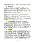 sandpiper, Common snipe, Marbled murrelet, Rufous hummingbird,
Belted kingfisher, Pacific slope flycatcher, Tree swallow, Barn
swallow, Steller's jay, Northwest crow, Raven, and other creepers
including wrens, vireos, sparrows, finches, pipits, kinglets, &
dippers. (FEIS V-l, 3-56). Sensitive species include: spotted
and rock sandpipers, dunlin, marbled murrelets, bald eagles,
sharp-shinned hawks, great horned owls, three-toed woodpeckers,
belted kingfishers, olive-sided and Pacific slope flycatchers,
western wood peewees, and dozens of other locally-breeding
species of passerines. (Fish and Wildlife Coordination Act
letter from Nevin Holmberg to Colonel William Kakel dated March
28, 1991).
In addition to birds, other common species found in the area
include black bear, mountain goat, Sitka black-tailed deer,
beaver, marten, 'river otter, mink, ermine and other mustelids,
lynx, red fox, hoary marmot, porcupine, and a number of other.
small mammals. (Fish and Wildlife Coordination Act letter from
Nevin Holmberg to Colonel William Kakel dated March 28, 1991).
Bird and other species may, or may not remain in the area
depending on disturbance from human activity, and cover and
foraging provided at the impoundment's margins. Certainly the
lack of deciduous trees following project construction means that
fewer passerines would nest in the valley. More and various
types of waterfowl would likely be attracted to the impoundment.
E. Ecological Risk Analysis
Analysis of potential effects of the post-operation
impoundment on local biota were based on estimates of contaminant
concentrations in the impoundment sediment, pore water (i.e.,
water in the pore spaces within the tailings) , and water column
as provided in Chapter VI of this report.
A preponderance-of-evidence approach was used. Adverse
effects on biota from contaminants in pore water and the water
column were estimated by comparing concentrations with Ambient
Water Quality Criteria (adjusted for hardness, pH, and
temperature where appropriate; 40 CFR Part 131, 1992) and aquatic
toxicity data. Effects of contaminants in sediments on benthic
biota were estimated by comparing sediment concentrations with
Canadian Provincial sediment quality guidelines (Ecology 1991,
Jaagumagi, 1993) , Wisconsin Department of Natural Resources
guidelines (Ecology 1991), and draft Great Lakes Effects Range
Medians (pers. comm., Ingersoll 1994). Potential effects on
wildlife from contaminants in the pore water, sediment, and water
column were estimated by constructing models to compare the
exposure of sandpipers, river otters, and kingfishers with the
potential toxicity from cadmium, lead, mercury, and selenium.
These metals were selected following discussion with EPA ORD
128
image:
sandpiper, Common snipe, Marbled murrelet, Rufous hummingbird,
Belted kingfisher, Pacific slope flycatcher, Tree swallow, Barn
swallow, Steller's jay, Northwest crow, Raven, and other creepers
including wrens, vireos, sparrows, finches, pipits, kinglets, &
dippers. (FEIS V-l, 3-56). Sensitive species include: spotted
and rock sandpipers, dunlin, marbled murrelets, bald eagles,
sharp-shinned hawks, great horned owls, three-toed woodpeckers,
belted kingfishers, olive-sided and Pacific slope flycatchers,
western wood peewees, and dozens of other locally-breeding
species of passerines. (Fish and Wildlife Coordination Act
letter from Nevin Holmberg to Colonel William Kakel dated March
28, 1991).
In addition to birds, other common species found in the area
include black bear, mountain goat, Sitka black-tailed deer,
beaver, marten, 'river otter, mink, ermine and other mustelids,
lynx, red fox, hoary marmot, porcupine, and a number of other.
small mammals. (Fish and Wildlife Coordination Act letter from
Nevin Holmberg to Colonel William Kakel dated March 28, 1991).
Bird and other species may, or may not remain in the area
depending on disturbance from human activity, and cover and
foraging provided at the impoundment's margins. Certainly the
lack of deciduous trees following project construction means that
fewer passerines would nest in the valley. More and various
types of waterfowl would likely be attracted to the impoundment.
E. Ecological Risk Analysis
Analysis of potential effects of the post-operation
impoundment on local biota were based on estimates of contaminant
concentrations in the impoundment sediment, pore water (i.e.,
water in the pore spaces within the tailings) , and water column
as provided in Chapter VI of this report.
A preponderance-of-evidence approach was used. Adverse
effects on biota from contaminants in pore water and the water
column were estimated by comparing concentrations with Ambient
Water Quality Criteria (adjusted for hardness, pH, and
temperature where appropriate; 40 CFR Part 131, 1992) and aquatic
toxicity data. Effects of contaminants in sediments on benthic
biota were estimated by comparing sediment concentrations with
Canadian Provincial sediment quality guidelines (Ecology 1991,
Jaagumagi, 1993) , Wisconsin Department of Natural Resources
guidelines (Ecology 1991), and draft Great Lakes Effects Range
Medians (pers. comm., Ingersoll 1994). Potential effects on
wildlife from contaminants in the pore water, sediment, and water
column were estimated by constructing models to compare the
exposure of sandpipers, river otters, and kingfishers with the
potential toxicity from cadmium, lead, mercury, and selenium.
These metals were selected following discussion with EPA ORD
128
image:
 (pers. comm., Norton 1994) because integrative assessments of
their toxicity and exposure pathways relevant to wildlife exist
(Eisler 1985a, 1985b, 1987, 1988) and because these have the
potential to bioaccumulate. The Wildlife Exposure Factors
Handbook (EPA 1993b) was used to derive many of the wildlife
exposure parameters. Additional information was used to evaluate
mercury (EPA 1993a) and selenium (Saiki 1986) . The data used are
considered reasonable and representative.
F. Evaluation of Contaminants in Pore Water
Predicted pore water concentrations for various contaminants
are shown in Tables 25 and 26. Contaminants of particular
concern included metals, cyanide, the breakdown products of
cyanide (thiocyanate, cyanate, and ammonia), and the xanthates (a
collecting agent added to the milling process; Hawley, 1977). It
is recognized here that water quality criteria are generally
designed to be protective of water column species and that
benthic organisms may or may not be similarly protected. It is
not unrealistic to assume, however, that certain species of fish
will be exposed to pore water or that fish or other water column
species can be useful indicators of pore water toxicity.
Therefore, in this analysis all data encountered for freshwater
organisms are included in the evaluation of potential toxicity of
the pore water in the tailings impoundment.
ii. Pore Water Evaluated Using Water Quality Criteria
Water Quality Criteria were available for most metals,
cyanide, and ammonia. Several of the metals criteria were
dependent on water hardness. The hardness value used (670 mg/L
CaCO3) was that predicted from the decant studies as described in
Chapter VI. Cyanide criteria are based on measurements of free
cyanide because this form is a much more reliable index of
toxicity to aquatic life than total cyanide since the latter can
include nitriles and more stable metallocyanide complexes.
However, because these complexes can dissociate as a function of
pH in the range that commonly occurs in many water bodies, total
cyanide is recommended for evaluation with the criteria
especially if only a few measurements are made on a water body
(EPA 1985- 440/5-84-028). For this analysis, the cyanide
criteria were applied to both free and total cyanide. It should
be noted that weak cyanide concentrations are more toxic to fish
at temperatures near freezing since HCN will not evaporate from
the surface of a waterbody when it is covered with ice; winter
129
image:
(pers. comm., Norton 1994) because integrative assessments of
their toxicity and exposure pathways relevant to wildlife exist
(Eisler 1985a, 1985b, 1987, 1988) and because these have the
potential to bioaccumulate. The Wildlife Exposure Factors
Handbook (EPA 1993b) was used to derive many of the wildlife
exposure parameters. Additional information was used to evaluate
mercury (EPA 1993a) and selenium (Saiki 1986) . The data used are
considered reasonable and representative.
F. Evaluation of Contaminants in Pore Water
Predicted pore water concentrations for various contaminants
are shown in Tables 25 and 26. Contaminants of particular
concern included metals, cyanide, the breakdown products of
cyanide (thiocyanate, cyanate, and ammonia), and the xanthates (a
collecting agent added to the milling process; Hawley, 1977). It
is recognized here that water quality criteria are generally
designed to be protective of water column species and that
benthic organisms may or may not be similarly protected. It is
not unrealistic to assume, however, that certain species of fish
will be exposed to pore water or that fish or other water column
species can be useful indicators of pore water toxicity.
Therefore, in this analysis all data encountered for freshwater
organisms are included in the evaluation of potential toxicity of
the pore water in the tailings impoundment.
ii. Pore Water Evaluated Using Water Quality Criteria
Water Quality Criteria were available for most metals,
cyanide, and ammonia. Several of the metals criteria were
dependent on water hardness. The hardness value used (670 mg/L
CaCO3) was that predicted from the decant studies as described in
Chapter VI. Cyanide criteria are based on measurements of free
cyanide because this form is a much more reliable index of
toxicity to aquatic life than total cyanide since the latter can
include nitriles and more stable metallocyanide complexes.
However, because these complexes can dissociate as a function of
pH in the range that commonly occurs in many water bodies, total
cyanide is recommended for evaluation with the criteria
especially if only a few measurements are made on a water body
(EPA 1985- 440/5-84-028). For this analysis, the cyanide
criteria were applied to both free and total cyanide. It should
be noted that weak cyanide concentrations are more toxic to fish
at temperatures near freezing since HCN will not evaporate from
the surface of a waterbody when it is covered with ice; winter
129
image:
 Table 25. Comparison of projected pore water concentrations with ambient water quality
an A or C respectively. Ratios that exceed
Hardness 670 mg/L
pH units 8.2
Pore Water
Concentration
Parameter ug/L
Ag 50
A^ffl) 14
Cd 10 C|
CKin) 20
Cr(VD 20 A
Cu 1300 A
Fe 850
Hg 5 A|
Mn 2700
Ni 30
Pb 20
Se 16 C|
Zn 87
mg/L
CNfree 1.1 A
CNtot 2.5
NH3 18 A
unity are also
• ••• *»•
enclo
Water Quality
Criterion (a)
Acute
107
360
34
8246
16
106
2.4
7089
919
20
586
0.02
0.02
pH
oC 7.4 8.2
1 16.0 4.1
4 15.3 3.9
7 14.8 3.8
Chronic
190
5
• 1003
11
60
1000
0.012
788
36
5
531
0.0052
0.0052
pH
7.4 8.2
2.1
2.0
1.9
0.8
0.8
0.7
Ratio of Parameter to
Criterion Concentration
Acute
Chronic
8.8
9.1
9.5
23
24
24
(a) Based on hardness of 670 and Water Effects Ratio of 1, following EPA 1992; As(in), Cr(VI), Hg, Fe, Se.
CN, and NH3 are not dependent on hardness; see discussion in text on application of Water Quality
Criteria to CNfree, CNtot, and NH3.
image:
Table 25. Comparison of projected pore water concentrations with ambient water quality
an A or C respectively. Ratios that exceed
Hardness 670 mg/L
pH units 8.2
Pore Water
Concentration
Parameter ug/L
Ag 50
A^ffl) 14
Cd 10 C|
CKin) 20
Cr(VD 20 A
Cu 1300 A
Fe 850
Hg 5 A|
Mn 2700
Ni 30
Pb 20
Se 16 C|
Zn 87
mg/L
CNfree 1.1 A
CNtot 2.5
NH3 18 A
unity are also
• ••• *»•
enclo
Water Quality
Criterion (a)
Acute
107
360
34
8246
16
106
2.4
7089
919
20
586
0.02
0.02
pH
oC 7.4 8.2
1 16.0 4.1
4 15.3 3.9
7 14.8 3.8
Chronic
190
5
• 1003
11
60
1000
0.012
788
36
5
531
0.0052
0.0052
pH
7.4 8.2
2.1
2.0
1.9
0.8
0.8
0.7
Ratio of Parameter to
Criterion Concentration
Acute
Chronic
8.8
9.1
9.5
23
24
24
(a) Based on hardness of 670 and Water Effects Ratio of 1, following EPA 1992; As(in), Cr(VI), Hg, Fe, Se.
CN, and NH3 are not dependent on hardness; see discussion in text on application of Water Quality
Criteria to CNfree, CNtot, and NH3.
image:
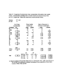 Table 26. Comparison of projected pore water concentrations with aquatic toxicity data.
Parameter concentrations exceeding aquatic values of concern are enclosed in boxes.
Ratios that exceed unity are also enclosed in boxes.
Pore Water
Concentration
Parameter mg/L
Concentration Range
of Concern (a)
High Low
Ratio of Parameter to
Concentration of Concern
High Low
CNS
Thiocyanate
CNO
Cyanate
Xanthates
390
73
24
95
5.6
1
18
0.01
0.8
0.2
(a) See discussion in text on estimation of high and low concentrations of concern for CNS, CNO,
and Xanthates. Note that the concentration ranges of concern would be much lower if based
on sublethal, chronic effects.
image:
Table 26. Comparison of projected pore water concentrations with aquatic toxicity data.
Parameter concentrations exceeding aquatic values of concern are enclosed in boxes.
Ratios that exceed unity are also enclosed in boxes.
Pore Water
Concentration
Parameter mg/L
Concentration Range
of Concern (a)
High Low
Ratio of Parameter to
Concentration of Concern
High Low
CNS
Thiocyanate
CNO
Cyanate
Xanthates
390
73
24
95
5.6
1
18
0.01
0.8
0.2
(a) See discussion in text on estimation of high and low concentrations of concern for CNS, CNO,
and Xanthates. Note that the concentration ranges of concern would be much lower if based
on sublethal, chronic effects.
image:
 conditions can increase the risk of fish kills by cyanides
(Palmes, 1993). Weak acid dissociable cyanide (CNwad) is a
measure of free cyanide plus cyanide bound to other metals,
especially copper, nickel, and zinc. CNwad is a measure of those
forms of cyanide considered to be toxicologically significant
(Smith and Mudder, 1991). For the pore water, the predicted
CNwad is equal to the predicted free cyanide, indicating that
there will not be much metal-bound cyanide and that evaluation of
free cyanide will be sufficient to evaluate CNwad. Ammonia
criteria depend on both pH and temperature. The pH values used
here ranged from 7.4 (which was reported as a background value;
Lakefield 1990, No. 3980, Table 7) to 8.2 (a value projected for
pore water; see Table 25). The temperatures used here ranged
from 1 oC (the impoundment is expected to freeze in the winter;
HDR) to 7 oC (expected in the bottom water in summer; HDR, 1990).
The estimated pore water concentrations were compared with both
acute and chronic criteria.
2. ' Pore Water Evaluated Using Aquatic Toxicity Data
Palmes (1993) review reported thiocyanate toxicity in fish
occurs over a range from 24 mg/L to 5,000 mg/L. In addition, if
fish are stressed (e.g., chased), mortality can increase after
exposure to as little as 5.5-7.7 mg/L. Heming et al. (1985)
found 10 to 100% mortality in stressed versus non-stressed brook
trout exposed to these lower concentrations. They also found
that, at 1.0 mg/L, rainbow trout accumulated thiocyanate at a
rate that would put 50% of the exposed population at risk of
lethal effects following a one to two month exposure. More
recently, Kevan and Dixon (1991) reported that exposures of 85
mg/L produce increased deformities in developing embryos of
rainbow trout. Green et al (1990) reported 50% reduction in
feeding by freshwater snails exposed to 5 mg/L. Smith and Mudder
(1991) reported a range of LC50s for fish from 50-200 mg/L. For
this analysis, 1.0 mg/L is used as a low (approximately
"chronic") concentration of concern and 24 mg/L as a higher
concentration. A no effect level of thiocyanate is likely to be
lower than 1.0 mg/L.
The toxicity of the predicted cyanate concentration was
evaluated using several sources. Cyanate is reported to be
1/1,000 as toxic as free cyanide (Response to comments 94.21;
Kensington project EIS) which suggests levels of 5.2 and 22 mg/L
(based on Water Quality Criteria for cyanide) might be
protective. Palmes (1993) review of cyanate toxicity suggests a
lower limit of 75 mg/L for fish (lethal to creek chub) which is
expected to be even lower for salmonids, based on salmonid
sensitivity to cyanide. Crustaceans experience mortality at 18
mg/L (Dauchy et al., 1980). Although cyanate is considered more
toxic than thiocyanate (Smith and Mudder, 1991), its toxicity is
affected by hardness (reports exist of both dramatic decreases
and moderate increases with hardness). LC50s for fish range from
132
image:
conditions can increase the risk of fish kills by cyanides
(Palmes, 1993). Weak acid dissociable cyanide (CNwad) is a
measure of free cyanide plus cyanide bound to other metals,
especially copper, nickel, and zinc. CNwad is a measure of those
forms of cyanide considered to be toxicologically significant
(Smith and Mudder, 1991). For the pore water, the predicted
CNwad is equal to the predicted free cyanide, indicating that
there will not be much metal-bound cyanide and that evaluation of
free cyanide will be sufficient to evaluate CNwad. Ammonia
criteria depend on both pH and temperature. The pH values used
here ranged from 7.4 (which was reported as a background value;
Lakefield 1990, No. 3980, Table 7) to 8.2 (a value projected for
pore water; see Table 25). The temperatures used here ranged
from 1 oC (the impoundment is expected to freeze in the winter;
HDR) to 7 oC (expected in the bottom water in summer; HDR, 1990).
The estimated pore water concentrations were compared with both
acute and chronic criteria.
2. ' Pore Water Evaluated Using Aquatic Toxicity Data
Palmes (1993) review reported thiocyanate toxicity in fish
occurs over a range from 24 mg/L to 5,000 mg/L. In addition, if
fish are stressed (e.g., chased), mortality can increase after
exposure to as little as 5.5-7.7 mg/L. Heming et al. (1985)
found 10 to 100% mortality in stressed versus non-stressed brook
trout exposed to these lower concentrations. They also found
that, at 1.0 mg/L, rainbow trout accumulated thiocyanate at a
rate that would put 50% of the exposed population at risk of
lethal effects following a one to two month exposure. More
recently, Kevan and Dixon (1991) reported that exposures of 85
mg/L produce increased deformities in developing embryos of
rainbow trout. Green et al (1990) reported 50% reduction in
feeding by freshwater snails exposed to 5 mg/L. Smith and Mudder
(1991) reported a range of LC50s for fish from 50-200 mg/L. For
this analysis, 1.0 mg/L is used as a low (approximately
"chronic") concentration of concern and 24 mg/L as a higher
concentration. A no effect level of thiocyanate is likely to be
lower than 1.0 mg/L.
The toxicity of the predicted cyanate concentration was
evaluated using several sources. Cyanate is reported to be
1/1,000 as toxic as free cyanide (Response to comments 94.21;
Kensington project EIS) which suggests levels of 5.2 and 22 mg/L
(based on Water Quality Criteria for cyanide) might be
protective. Palmes (1993) review of cyanate toxicity suggests a
lower limit of 75 mg/L for fish (lethal to creek chub) which is
expected to be even lower for salmonids, based on salmonid
sensitivity to cyanide. Crustaceans experience mortality at 18
mg/L (Dauchy et al., 1980). Although cyanate is considered more
toxic than thiocyanate (Smith and Mudder, 1991), its toxicity is
affected by hardness (reports exist of both dramatic decreases
and moderate increases with hardness). LC50s for fish range from
132
image:
 13-82 mg/L, but concentrations of 85 mg/L at hardness greater
than 200 mg/L have shown no mortality, even though another study
found an LC50 at 24 mg/L for hardness of 250 mg/L and an LC50 of
95 mg/L for hardness of 200 mg/L. The low to high range chosen
for this analysis is from 18 mg/L (for crustaceans) to 95 mg/L
(high hardness, and one of the highest LCSOs)..
A search of EPA's AQUIRE (Aquatic toxicity information
retrieval) database on 2/15/94 yielded information on six
different xanthates. The crustacean Daphnia magna was generally
the most sensitive organism. Immobility in this species was
reported at concentrations from 0.35 to 3.7 mg/L (for sodium
ethyl and sodium isopropyl xanthate, respectively). Rainbow
trout exhibited mortality over a concentration range from 0.3 to
180 mg/L for sodium isopropyl xanthate, but LCSOs ranged from 13
to 320 mg/L for other xanthates. Hawley (1977) summarized
effects of a variety of xanthates on Daphnia, a shiner, and
fathead minnow. Daphnia was consistently most susceptible;
xanthates were generally described as having high toxicity
eliciting effects in the range from 0.1 to 1.0 mg/L or from 0.56
to 10 mg/L. The shiner's susceptibility varied depending on the
specific xanthate. Sodium isopropyl, sodium ethyl, and potassium
ethyl xanthate had high toxicity (0.01 to 0.1 mg/L), whereas
sodium isobutyl and potassium amyl xanthate had moderate toxicity
(10 to 100 mg/L). The fathead minnow had the widest range of
susceptibility. Susceptibility was greatest for sodium
isopropyl, sodium ethyl, and potassium ethyl xanthate
(approximately 0.1 to 1.0 or 0.18 to 1.8 mg/L) and least for
potassium hexyl xanthate (100 to 1000 mg/L). The range selected
for analysis here is from 0.01 (effects on shiner by three
xanthates) to 5.6 (median of upper ranges of effects reported by
Hawley (1977). This range encompasses much of the AQUIRE data
for sensitive species.
G.. Results of Pore Water Evaluation
The pore water can be characterized as potentially highly
toxic based on the analysis presented here (note how exceedances
for Hg and cyanide are more than two orders of magnitude above
chronic water quality criteria). Tables 25 and 26 summarize the
results of comparing projected pore water concentrations with
water quality criteria and aquatic toxicity data. These results
indicate that several of the metals (Cu, Hg, and Cr if it is
present exclusively as Cr(VI)), cyanide, and ammonia would exceed
applicable acute water quality criteria and that thiocyanate
would occur at a level likely to be associated with aquatic
toxicity. In addition, Cd, Se, cyanate, and xanthates are of
concern due to exceedance of chronic water quality criteria or
more conservative concentrations associated.with aquatic
toxicity.
133
image:
13-82 mg/L, but concentrations of 85 mg/L at hardness greater
than 200 mg/L have shown no mortality, even though another study
found an LC50 at 24 mg/L for hardness of 250 mg/L and an LC50 of
95 mg/L for hardness of 200 mg/L. The low to high range chosen
for this analysis is from 18 mg/L (for crustaceans) to 95 mg/L
(high hardness, and one of the highest LCSOs)..
A search of EPA's AQUIRE (Aquatic toxicity information
retrieval) database on 2/15/94 yielded information on six
different xanthates. The crustacean Daphnia magna was generally
the most sensitive organism. Immobility in this species was
reported at concentrations from 0.35 to 3.7 mg/L (for sodium
ethyl and sodium isopropyl xanthate, respectively). Rainbow
trout exhibited mortality over a concentration range from 0.3 to
180 mg/L for sodium isopropyl xanthate, but LCSOs ranged from 13
to 320 mg/L for other xanthates. Hawley (1977) summarized
effects of a variety of xanthates on Daphnia, a shiner, and
fathead minnow. Daphnia was consistently most susceptible;
xanthates were generally described as having high toxicity
eliciting effects in the range from 0.1 to 1.0 mg/L or from 0.56
to 10 mg/L. The shiner's susceptibility varied depending on the
specific xanthate. Sodium isopropyl, sodium ethyl, and potassium
ethyl xanthate had high toxicity (0.01 to 0.1 mg/L), whereas
sodium isobutyl and potassium amyl xanthate had moderate toxicity
(10 to 100 mg/L). The fathead minnow had the widest range of
susceptibility. Susceptibility was greatest for sodium
isopropyl, sodium ethyl, and potassium ethyl xanthate
(approximately 0.1 to 1.0 or 0.18 to 1.8 mg/L) and least for
potassium hexyl xanthate (100 to 1000 mg/L). The range selected
for analysis here is from 0.01 (effects on shiner by three
xanthates) to 5.6 (median of upper ranges of effects reported by
Hawley (1977). This range encompasses much of the AQUIRE data
for sensitive species.
G.. Results of Pore Water Evaluation
The pore water can be characterized as potentially highly
toxic based on the analysis presented here (note how exceedances
for Hg and cyanide are more than two orders of magnitude above
chronic water quality criteria). Tables 25 and 26 summarize the
results of comparing projected pore water concentrations with
water quality criteria and aquatic toxicity data. These results
indicate that several of the metals (Cu, Hg, and Cr if it is
present exclusively as Cr(VI)), cyanide, and ammonia would exceed
applicable acute water quality criteria and that thiocyanate
would occur at a level likely to be associated with aquatic
toxicity. In addition, Cd, Se, cyanate, and xanthates are of
concern due to exceedance of chronic water quality criteria or
more conservative concentrations associated.with aquatic
toxicity.
133
image:
 H* Evaluation, of Contaminants in Sediments
Contaminant concentrations in sediment (see Table 27) are
expressed as ing-contaminant/kg-sediment dry weight. Potential
toxicity of metals and cyanide in the impoundment sediments was
evaluated using available "benchmarks" also based on dry weight.
Each of these benchmarks has limitations, but when taken
together, they provide an indication of which contaminants are
likely to exert adverse effects on any kind of benthic community
that may develop on and in the impoundment sediments. Two sets
of benchmarks were taken from the summary provided in Ecology
(1991). First, were the Provincial Sediment Quality Guidelines
(both a lowest effect and a severe effect, with benchmarks for
silver and cyanide based on dredged disposal criteria) and,
second, the Wisconsin Department of Natural Resources benchmark
numbers (Ecology, 1991, discusses the basis and limitations of
these benchmarks). A third set of draft numbers was provided by
the Great Lakes Program (C. Ingersoll, pers. comm.). These
preliminary numbers are the effects range medians (ERMs) for
associations between total metals (dry weight) in whole sediment
samples from the Great Lakes and other regions and toxicity to
the freshwater amphipod, Hyallela azteca. These numbers are
based on approximately 60 to 70 samples and are used here only
for those metals for which the ERM could correctly classify
samples as having effects or not, 70 to 80 per cent of the time.
It must be noted that the numbers used here are only preliminary
and are subject to some final adjustment.
Results of comparing predicted sediment concentrations of
metals and cyanide with three sets of benchmarks for freshwater
sediments are presented in Table 27. All parameters are expected
to exceed at least one of the benchmarks. Contaminants of
particular concern include cyanide, copper, and cadmium, which
exceeded benchmarks by over an order of magnitude (consistently
so for cadmium). Lead, too, exceeded all three benchmarks. In
general, these comparisons indicate moderate to very high levels
of toxicity will be present in the tailings sediments (note that
all parameters evaluated exceeded the Provincial SQ Guidelines
for a lowest-effect).
!_._ Evaluation of Metals in the Water Column
Metals concentrations in the water column were predicted
using the WASP4 model as described in Chapter VI. The same
adjustments for hardness were made as done previously for the
pore water (for cadmium, copper, lead, and zinc).
The modeling results predicted virtually identical values
for dissolved and total metals in the water column (Table 28),
suggesting very little metal would be bound to suspended
sediments. It should be noted, however, that this analysis
134
image:
H* Evaluation, of Contaminants in Sediments
Contaminant concentrations in sediment (see Table 27) are
expressed as ing-contaminant/kg-sediment dry weight. Potential
toxicity of metals and cyanide in the impoundment sediments was
evaluated using available "benchmarks" also based on dry weight.
Each of these benchmarks has limitations, but when taken
together, they provide an indication of which contaminants are
likely to exert adverse effects on any kind of benthic community
that may develop on and in the impoundment sediments. Two sets
of benchmarks were taken from the summary provided in Ecology
(1991). First, were the Provincial Sediment Quality Guidelines
(both a lowest effect and a severe effect, with benchmarks for
silver and cyanide based on dredged disposal criteria) and,
second, the Wisconsin Department of Natural Resources benchmark
numbers (Ecology, 1991, discusses the basis and limitations of
these benchmarks). A third set of draft numbers was provided by
the Great Lakes Program (C. Ingersoll, pers. comm.). These
preliminary numbers are the effects range medians (ERMs) for
associations between total metals (dry weight) in whole sediment
samples from the Great Lakes and other regions and toxicity to
the freshwater amphipod, Hyallela azteca. These numbers are
based on approximately 60 to 70 samples and are used here only
for those metals for which the ERM could correctly classify
samples as having effects or not, 70 to 80 per cent of the time.
It must be noted that the numbers used here are only preliminary
and are subject to some final adjustment.
Results of comparing predicted sediment concentrations of
metals and cyanide with three sets of benchmarks for freshwater
sediments are presented in Table 27. All parameters are expected
to exceed at least one of the benchmarks. Contaminants of
particular concern include cyanide, copper, and cadmium, which
exceeded benchmarks by over an order of magnitude (consistently
so for cadmium). Lead, too, exceeded all three benchmarks. In
general, these comparisons indicate moderate to very high levels
of toxicity will be present in the tailings sediments (note that
all parameters evaluated exceeded the Provincial SQ Guidelines
for a lowest-effect).
!_._ Evaluation of Metals in the Water Column
Metals concentrations in the water column were predicted
using the WASP4 model as described in Chapter VI. The same
adjustments for hardness were made as done previously for the
pore water (for cadmium, copper, lead, and zinc).
The modeling results predicted virtually identical values
for dissolved and total metals in the water column (Table 28),
suggesting very little metal would be bound to suspended
sediments. It should be noted, however, that this analysis
134
image:
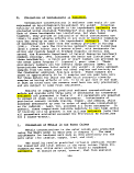 Table 27. Comparison of projected sediment concentrations of metals and cyanide with several potential
freshwater sediment benchmarks (Provincial Sediment Quality Guidelines, Wisconsin DNR benchmarks,
and draft Great Lakes Effects Range Median for a freshwater amphipod). Concentrations exceeding at
least one benchmark are enclosed in boxes. Ratios (concentration/benchmark) from 1-10 are enclosed
in lightly outlined boxes; ratios greater than 10 are enclosed in heavily outlined boxes.
Impoundment
Sediments
Parameter mg/kg
Ag
As
Cd
Cr
Cu
Fe
Hg
Mn
Ni
Pb
Se
Zn
CNtot
3
9.8
11
35
260
46,000
0.27
1600
26
200
1
530
42.4
Provincial SQ Guidelines (a)
Lowest-Effect Severe-Effect
mg/kg
0.5
6
0.6
26
16
20,000
0.2
460
16
31
120
Ratio
6
1.6
"IT
1.3
~16~
2.3
1.4
3.5
1.6
6.5
4.4
mg/kg
33
10
110
110
40,000
2
1100
75
250
820
Ratio
0.3
1.1
0.3
2.4
1.2
0.1
1.5
0.3
0.8
0.6
WI DNR(b)
mg/kg Ratio
10
1
100
100
1.0
11
0.4
2.6
0.11 2.7
100
50
1
100
0.3
~~4~
1
5.3
Draft Great Lakes
ERM(c)
mg/kg Ratio
(a) - Dry weight basis. Taken from Jaagumagi, 1993, and Ecology, 1991. Ag &.CN numbers from Dredged Disposal Criteria
(b) - Taken fiom Ecology, 1991. Based on background
(c) - Preliminary Effects Range Medians for associations between total metals (dry wt) in whole sediment samples from the Great l^kes
and other regions and toxicity to Hyallela azteca. Based on approximately 60-70 samples. Results for contaminants
for which the ERM could correctly classify samples 70-80% of the time (C. Ingersoll, pers. comm. 05/11/94. Note that
the numbers presented here are only preliminary and subject to some final adjustment).
image:
Table 27. Comparison of projected sediment concentrations of metals and cyanide with several potential
freshwater sediment benchmarks (Provincial Sediment Quality Guidelines, Wisconsin DNR benchmarks,
and draft Great Lakes Effects Range Median for a freshwater amphipod). Concentrations exceeding at
least one benchmark are enclosed in boxes. Ratios (concentration/benchmark) from 1-10 are enclosed
in lightly outlined boxes; ratios greater than 10 are enclosed in heavily outlined boxes.
Impoundment
Sediments
Parameter mg/kg
Ag
As
Cd
Cr
Cu
Fe
Hg
Mn
Ni
Pb
Se
Zn
CNtot
3
9.8
11
35
260
46,000
0.27
1600
26
200
1
530
42.4
Provincial SQ Guidelines (a)
Lowest-Effect Severe-Effect
mg/kg
0.5
6
0.6
26
16
20,000
0.2
460
16
31
120
Ratio
6
1.6
"IT
1.3
~16~
2.3
1.4
3.5
1.6
6.5
4.4
mg/kg
33
10
110
110
40,000
2
1100
75
250
820
Ratio
0.3
1.1
0.3
2.4
1.2
0.1
1.5
0.3
0.8
0.6
WI DNR(b)
mg/kg Ratio
10
1
100
100
1.0
11
0.4
2.6
0.11 2.7
100
50
1
100
0.3
~~4~
1
5.3
Draft Great Lakes
ERM(c)
mg/kg Ratio
(a) - Dry weight basis. Taken from Jaagumagi, 1993, and Ecology, 1991. Ag &.CN numbers from Dredged Disposal Criteria
(b) - Taken fiom Ecology, 1991. Based on background
(c) - Preliminary Effects Range Medians for associations between total metals (dry wt) in whole sediment samples from the Great l^kes
and other regions and toxicity to Hyallela azteca. Based on approximately 60-70 samples. Results for contaminants
for which the ERM could correctly classify samples 70-80% of the time (C. Ingersoll, pers. comm. 05/11/94. Note that
the numbers presented here are only preliminary and subject to some final adjustment).
image:
 Table 28. Comparison of projected water column concentrations (from Tables 12 & 13) with ambient
water quality criteria. Concentrations exceeding acute or chronic criteria and ratios exceeding unity
are enclosed in boxes.
Scenarios 1-12
Impoundment
Water Column Water
Quality
Concentration Criterion (a)
Dissolved
Parameter ug/L
AsOOI) 0.06
Cd 0.05
.CrOID 0.09
Cr(VI) 0.09
Cu 5.9
Hg 0.022
Pb 0.084
Se 0.072
Zn 0.387
Total Acute
ug/L ug/L
0.06 360
0.05 34
0.09 8246
0.09 16
5.9 106
0.022 | 2.4
0.084 919
0.072 20
0.387 586
Chronic
ug/L
190
5
1003
11
60
0.012
36
5
531
Ratio of Parameter to
Criterion Concentration
Acute Chronic
0.0
0.0
0.0
0.0
0.1
0.0 [
0.0
0.0
0.0
0.0
0.0
0.0
0.0
0.1
1.8)
0.0
0.0
0.0
Scenario 13 - Includes bioturbation
AsOH) 0.61
Cd 0.43
CrOID 0.84
Cr(VI) 0.84
Cu 56
Hg 0.215
Pb 0.844
Se 0.686
Zn 3.7
0.61 360
0.43 34
0.84 8246
0.84 16
56 106
0.215 2.4
0.844 919
0.686 20
3.7 586
190
5
1003
11
60
0.012
36
5
531
0.0
0.0
0.0
o.i.
0.5
0.1 [
0.0
0.0
0.0
0.0
0.1
0.0
0.1
0.9
18]
0.0
0.1
0.0
Scenarios 14 A 15- Includes groundwater moving up through pore water into water column
As(in) 2
Cd 1.4
CrOID 2.8
CKVD 2.8
Cu 190
Hg 0.71
Pb 2.650
Se 2.29
Zn 11.9
2 360
1.4 34
2.8 8246
2.8 16
190 106
0.71 2.4
2.650 919
2.29 20
11.9 586
190
5
1003
11
60
0.012
36
5
531
0.0
0.0
0.0
0.2
) 18)
0.3
0.0
0.1
0.0
0.0
0.3
0.0
0.3
3.2
59
0.1
0.5
0.0
(a) Based on hardness of 670 and Water Effects Ratio of 1, following EPA 1992; As(in), Cr(VI), Hg, Fe, and Se
are not dependent on hardness; see discussion in text on application of Water Quality Criteria.
image:
Table 28. Comparison of projected water column concentrations (from Tables 12 & 13) with ambient
water quality criteria. Concentrations exceeding acute or chronic criteria and ratios exceeding unity
are enclosed in boxes.
Scenarios 1-12
Impoundment
Water Column Water
Quality
Concentration Criterion (a)
Dissolved
Parameter ug/L
AsOOI) 0.06
Cd 0.05
.CrOID 0.09
Cr(VI) 0.09
Cu 5.9
Hg 0.022
Pb 0.084
Se 0.072
Zn 0.387
Total Acute
ug/L ug/L
0.06 360
0.05 34
0.09 8246
0.09 16
5.9 106
0.022 | 2.4
0.084 919
0.072 20
0.387 586
Chronic
ug/L
190
5
1003
11
60
0.012
36
5
531
Ratio of Parameter to
Criterion Concentration
Acute Chronic
0.0
0.0
0.0
0.0
0.1
0.0 [
0.0
0.0
0.0
0.0
0.0
0.0
0.0
0.1
1.8)
0.0
0.0
0.0
Scenario 13 - Includes bioturbation
AsOH) 0.61
Cd 0.43
CrOID 0.84
Cr(VI) 0.84
Cu 56
Hg 0.215
Pb 0.844
Se 0.686
Zn 3.7
0.61 360
0.43 34
0.84 8246
0.84 16
56 106
0.215 2.4
0.844 919
0.686 20
3.7 586
190
5
1003
11
60
0.012
36
5
531
0.0
0.0
0.0
o.i.
0.5
0.1 [
0.0
0.0
0.0
0.0
0.1
0.0
0.1
0.9
18]
0.0
0.1
0.0
Scenarios 14 A 15- Includes groundwater moving up through pore water into water column
As(in) 2
Cd 1.4
CrOID 2.8
CKVD 2.8
Cu 190
Hg 0.71
Pb 2.650
Se 2.29
Zn 11.9
2 360
1.4 34
2.8 8246
2.8 16
190 106
0.71 2.4
2.650 919
2.29 20
11.9 586
190
5
1003
11
60
0.012
36
5
531
0.0
0.0
0.0
0.2
) 18)
0.3
0.0
0.1
0.0
0.0
0.3
0.0
0.3
3.2
59
0.1
0.5
0.0
(a) Based on hardness of 670 and Water Effects Ratio of 1, following EPA 1992; As(in), Cr(VI), Hg, Fe, and Se
are not dependent on hardness; see discussion in text on application of Water Quality Criteria.
image:
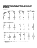 assumed no resuspension of bottom sediments. Potential effects
of resuspended sediments on wildlife is evaluated in a later
section. The results from comparing modeled concentrations of
contaminants in the water column with ambient water quality
criteria (Table 28) show that mercury is predicted to exceed the
chronic criterion. Furthermore these results show that when the
influence of bioturbation and groundwater flow (Scenarios 13-15)
are included in the modeling, copper concentrations are likely to
exceed the acute criterion as well.
J.. Evaluation of Potential Effects on Wildlife
JU_ Selection of Contaminants
Cadmium, mercury, selenium, and lead were selected, in
consultation with EPA-ORD (S. Norton, pers. comm.), as
contaminants of concern because of their potential to
bioaccumulate; bioconcentration factors (BCFs; concentration in
tissue [wet-weight] divided by concentration in water) for these
metals are generally greater than 1000 (see Table 29 below) .
Mercury in. particular, is of high concern. The mercury
concentration in pore water is projected to exceed the acute
water quality criterion (Table 25); sediment concentrations of
mercury are predicted to exceed two freshwater sediment
benchmarks (Table 27); and mercury in the water column is
projected to exceed the chronic water quality criterion (Table
28). Cadmium is expected to exceed all the freshwater sediment
benchmarks (Table 27) as well as the chronic water quality
criterion applied to pore water (Table 25). Selenium is
predicted to be at toxic levels in the pore water and sediment
(Tables 25 and 27) and Lead is expected to exceed several of the
freshwater sediment benchmarks (Table 27). These four metals
represent a range in level of concern for potential effects on
wildlife, with mercury of highest, selenium and lead lowest, and
cadmium in between. In addition, wildlife toxicity data for
these metals are available (Eisler, 1985a, 1985b, 1987, 1988).
2_._ Selection of Species
Three species, the kingfisher, spotted sandpiper, and river
otter, were selected in consultation with EPA-ORD (S. Norton,
pers. comm.). These species are expected to or are known to
inhabit the general Sheep Creek area (see Section D.6).
Information on conducting exposure assessments is available for
these three species (EPA, 1993b). The kingfisher was chosen to
represent a bird with a relatively small home range that feeds
primarily on fish. The sandpiper was chosen to represent a bird
that also forages along shorelines but has a high rate of
incidental ingestion of sediment. The river otter represents a
137
image:
assumed no resuspension of bottom sediments. Potential effects
of resuspended sediments on wildlife is evaluated in a later
section. The results from comparing modeled concentrations of
contaminants in the water column with ambient water quality
criteria (Table 28) show that mercury is predicted to exceed the
chronic criterion. Furthermore these results show that when the
influence of bioturbation and groundwater flow (Scenarios 13-15)
are included in the modeling, copper concentrations are likely to
exceed the acute criterion as well.
J.. Evaluation of Potential Effects on Wildlife
JU_ Selection of Contaminants
Cadmium, mercury, selenium, and lead were selected, in
consultation with EPA-ORD (S. Norton, pers. comm.), as
contaminants of concern because of their potential to
bioaccumulate; bioconcentration factors (BCFs; concentration in
tissue [wet-weight] divided by concentration in water) for these
metals are generally greater than 1000 (see Table 29 below) .
Mercury in. particular, is of high concern. The mercury
concentration in pore water is projected to exceed the acute
water quality criterion (Table 25); sediment concentrations of
mercury are predicted to exceed two freshwater sediment
benchmarks (Table 27); and mercury in the water column is
projected to exceed the chronic water quality criterion (Table
28). Cadmium is expected to exceed all the freshwater sediment
benchmarks (Table 27) as well as the chronic water quality
criterion applied to pore water (Table 25). Selenium is
predicted to be at toxic levels in the pore water and sediment
(Tables 25 and 27) and Lead is expected to exceed several of the
freshwater sediment benchmarks (Table 27). These four metals
represent a range in level of concern for potential effects on
wildlife, with mercury of highest, selenium and lead lowest, and
cadmium in between. In addition, wildlife toxicity data for
these metals are available (Eisler, 1985a, 1985b, 1987, 1988).
2_._ Selection of Species
Three species, the kingfisher, spotted sandpiper, and river
otter, were selected in consultation with EPA-ORD (S. Norton,
pers. comm.). These species are expected to or are known to
inhabit the general Sheep Creek area (see Section D.6).
Information on conducting exposure assessments is available for
these three species (EPA, 1993b). The kingfisher was chosen to
represent a bird with a relatively small home range that feeds
primarily on fish. The sandpiper was chosen to represent a bird
that also forages along shorelines but has a high rate of
incidental ingestion of sediment. The river otter represents a
137
image:
 Table 29. Bioconcentration factors for accumulation of mercury, cadmium, lead, and selenium from water into fish,
invertebrates, and amphibians.
Organism
Fish
Invertebrates
Amphibians
Fish
Invertebrates
Amphibians
Fish
Invertebrates
Amphibians
Fish
Invertebrates
Amphibians
BCF
Source
Mercury
95,000 EPA 1993a, p 2-7, methylHg in fish tissue is related to total Hg in water column, lists 60,000
and 130,000 depending on fish trophic status; average of 95,000 used here.
95,000 assume same as for fish; freshwater BCFs in EPA 1985 range from 300 to 8000, with marine
BCFs up to 350,000.
95,000 assume same as for fish
Cadmium
1,500 Eisler, I985a, p 27, for trout exposed for 3 months to 10 ug/L; mean of measurements made on
various tissues.
1,200 ibid., p 28; mean of 6 values for various species.
1,500 assume same as for fish
Selenium
1,000 Saiki, 1986, p 30, mean BCF for Kesterson was >1000. Eisler, 1985, reports 460 and 3,300 for
fish exposed to Se at up to 3.3 ug/L and 40 ug/L.
322 AQUIRE search, 5/5/94, for Daphnia exposed to 5 ug/L.
1,000 assume same as for fish
Lead
726 Eisler, 1988, p 61, for trout exposed for 7 days to 3.5 ug/L
5,000 Ibid., p 59; range from 1000 to 9000
726 assume same as for fish
image:
Table 29. Bioconcentration factors for accumulation of mercury, cadmium, lead, and selenium from water into fish,
invertebrates, and amphibians.
Organism
Fish
Invertebrates
Amphibians
Fish
Invertebrates
Amphibians
Fish
Invertebrates
Amphibians
Fish
Invertebrates
Amphibians
BCF
Source
Mercury
95,000 EPA 1993a, p 2-7, methylHg in fish tissue is related to total Hg in water column, lists 60,000
and 130,000 depending on fish trophic status; average of 95,000 used here.
95,000 assume same as for fish; freshwater BCFs in EPA 1985 range from 300 to 8000, with marine
BCFs up to 350,000.
95,000 assume same as for fish
Cadmium
1,500 Eisler, I985a, p 27, for trout exposed for 3 months to 10 ug/L; mean of measurements made on
various tissues.
1,200 ibid., p 28; mean of 6 values for various species.
1,500 assume same as for fish
Selenium
1,000 Saiki, 1986, p 30, mean BCF for Kesterson was >1000. Eisler, 1985, reports 460 and 3,300 for
fish exposed to Se at up to 3.3 ug/L and 40 ug/L.
322 AQUIRE search, 5/5/94, for Daphnia exposed to 5 ug/L.
1,000 assume same as for fish
Lead
726 Eisler, 1988, p 61, for trout exposed for 7 days to 3.5 ug/L
5,000 Ibid., p 59; range from 1000 to 9000
726 assume same as for fish
image:
 mammal that may. feed primarily on fish. The river otter is also
characterized as a "noteworthy indicator of bioaccumulative
pollution in aquatic ecosystems" and it is known to ingest mud
and other debris while probing and feeding in bottom sediments
(EPA, 1993b).
3. Selection of Exposure Pathways
Exposure of these three species to the four metals was
evaluated for the ingestion pathway which generally included: (1)
drinking the surface water including resuspended bottom sediments
at a concentration of 0.385 mg-sed-dry-wt/L (see Table 32; TSS),
(2) eating fish, invertebrates, and amphibians, and, where
appropriate, (3) incidental ingestion of sediments.
The kingfisher is expected to forage in relatively shallow
water, so that uptake from fish, invertebrates, and amphibians is
based on bioconcentration from contaminants in the water column.
The kingfisher is not expected to ingest any sediment other than
sediment present in its drinking water. An additional scenario
evaluated assumes the invertebrates consumed by the kingfisher
would come from the bottom of the impoundment where they would
bioaccumulate metals from the pore water (see Table 30).
The sandpiper would be expected to ingest sediments that are
resuspended and deposited in shallow areas along the shoreline.
It is assumed that these shoreline sediments would all come from
tailings. The diet of the sandpiper is assumed to be exclusively
invertebrates (see Table 33). Two scenarios are evaluated,
first, assuming invertebrates would not be exposed to pore water
and then assuming they would be exposed.
The river otter is expected to forage in deeper water, so
that uptake from invertebrates is based on bioconcentration from
contaminants in the pore water, whereas uptake from fish and
amphibians is based on bioconcentration of contaminants in the
water column. The river otter is also expected to ingest bottom
sediments. A second scenario assumes half of the invertebrates
consumed are from shallow areas and are not exposed to pore
water. .
Dermal absorption and inhalation pathways were not evaluated
because they are expected to have a low contribution to the total
exposure to the metals in the proposed impoundment.
Relevant data on exposure were taken from EPA (1993b) for each
of the species as discussed below.
4_^ Exposure of Wildlife to Metals
The general approach to evaluating exposure to the metals
was driven somewhat by the toxicity data available for
139
image:
mammal that may. feed primarily on fish. The river otter is also
characterized as a "noteworthy indicator of bioaccumulative
pollution in aquatic ecosystems" and it is known to ingest mud
and other debris while probing and feeding in bottom sediments
(EPA, 1993b).
3. Selection of Exposure Pathways
Exposure of these three species to the four metals was
evaluated for the ingestion pathway which generally included: (1)
drinking the surface water including resuspended bottom sediments
at a concentration of 0.385 mg-sed-dry-wt/L (see Table 32; TSS),
(2) eating fish, invertebrates, and amphibians, and, where
appropriate, (3) incidental ingestion of sediments.
The kingfisher is expected to forage in relatively shallow
water, so that uptake from fish, invertebrates, and amphibians is
based on bioconcentration from contaminants in the water column.
The kingfisher is not expected to ingest any sediment other than
sediment present in its drinking water. An additional scenario
evaluated assumes the invertebrates consumed by the kingfisher
would come from the bottom of the impoundment where they would
bioaccumulate metals from the pore water (see Table 30).
The sandpiper would be expected to ingest sediments that are
resuspended and deposited in shallow areas along the shoreline.
It is assumed that these shoreline sediments would all come from
tailings. The diet of the sandpiper is assumed to be exclusively
invertebrates (see Table 33). Two scenarios are evaluated,
first, assuming invertebrates would not be exposed to pore water
and then assuming they would be exposed.
The river otter is expected to forage in deeper water, so
that uptake from invertebrates is based on bioconcentration from
contaminants in the pore water, whereas uptake from fish and
amphibians is based on bioconcentration of contaminants in the
water column. The river otter is also expected to ingest bottom
sediments. A second scenario assumes half of the invertebrates
consumed are from shallow areas and are not exposed to pore
water. .
Dermal absorption and inhalation pathways were not evaluated
because they are expected to have a low contribution to the total
exposure to the metals in the proposed impoundment.
Relevant data on exposure were taken from EPA (1993b) for each
of the species as discussed below.
4_^ Exposure of Wildlife to Metals
The general approach to evaluating exposure to the metals
was driven somewhat by the toxicity data available for
139
image:
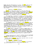 comparison. The toxicity data were of three kinds, doses (mg-
contaminant/kg-bw/day), dietary concentrations (mg-
contaminant/kg-food-wet-wt), and water concentrations (mg-
contaminant/L). Corresponding exposure data were developed for
the dose and dietary concentration scenarios as described below;
water concentrations considered safe to wildlife were compared
directly with the predicted water column concentrations. This
section refers repeatedly to the analyses done for the three
species (Tables 27-37) in terms of defining parameters and the
equations used to calculate exposure.
a. Ingested Doses
As discussed in detail in this section, consumption rates
were developed for water, food, and sediment ingestion on a body
weight basis. Parameters used in exposure calculations are found
in Tables 30, 33, 34, 36, and 39; data developed for the river
otter are used here to provide an example of the approach used.
Body weights (BW) and water ingestion rates (IRW) were taken
directly from EPA (1993b). Food ingestion rates (on a wet weight
basis, IRFW) were either taken .directly from EPA (1993b), or
estimated using the approach outlined in Figure 4-7 of that
document (this allows one to estimate food ingestion rate based
on free-living metabolic rate and dietary composition). Sediment
ingestion rates were estimated by multiplying the food ingestion
(wet weight) rate (IRFW) by the ratio of sediment to food (STF)
in the diet, as explained below.
i. Water Ingestion Rate and Dose
Water ingestion rates were available in EPA (1993b) . They
were multiplied by water column concentrations to obtain the dose
from drinking water (DW; mg-contaminant/kg-bw/day). The ingested
water will have suspended sediments in it and this contribution
is included in the present analysis. The separate estimate of
sediment ingestion is based on the amount of sediment measured in
scat samples and presumably integrates over all routes of
incidental sediment ingestion. Although the overall sediment
ingestion estimate may already include suspended sediment in the
drinking water, the separate estimates presented here allow a
comparison of the relative influence of this pathway (suspended
sediments in drinking water).
ii. Food Ingestion Rate and Dose
The overall food ingestion rate was taken either directly
from EPA (1993b) , or, as in the case of the river otter,
calculated following the example calculation in Figure 4-7 of
that document. Estimation of the food ingestion rate (IRFW; wet-
wt basis) for the river otter is shown in Table 36, which
calculates the rate as follows:
140
image:
comparison. The toxicity data were of three kinds, doses (mg-
contaminant/kg-bw/day), dietary concentrations (mg-
contaminant/kg-food-wet-wt), and water concentrations (mg-
contaminant/L). Corresponding exposure data were developed for
the dose and dietary concentration scenarios as described below;
water concentrations considered safe to wildlife were compared
directly with the predicted water column concentrations. This
section refers repeatedly to the analyses done for the three
species (Tables 27-37) in terms of defining parameters and the
equations used to calculate exposure.
a. Ingested Doses
As discussed in detail in this section, consumption rates
were developed for water, food, and sediment ingestion on a body
weight basis. Parameters used in exposure calculations are found
in Tables 30, 33, 34, 36, and 39; data developed for the river
otter are used here to provide an example of the approach used.
Body weights (BW) and water ingestion rates (IRW) were taken
directly from EPA (1993b). Food ingestion rates (on a wet weight
basis, IRFW) were either taken .directly from EPA (1993b), or
estimated using the approach outlined in Figure 4-7 of that
document (this allows one to estimate food ingestion rate based
on free-living metabolic rate and dietary composition). Sediment
ingestion rates were estimated by multiplying the food ingestion
(wet weight) rate (IRFW) by the ratio of sediment to food (STF)
in the diet, as explained below.
i. Water Ingestion Rate and Dose
Water ingestion rates were available in EPA (1993b) . They
were multiplied by water column concentrations to obtain the dose
from drinking water (DW; mg-contaminant/kg-bw/day). The ingested
water will have suspended sediments in it and this contribution
is included in the present analysis. The separate estimate of
sediment ingestion is based on the amount of sediment measured in
scat samples and presumably integrates over all routes of
incidental sediment ingestion. Although the overall sediment
ingestion estimate may already include suspended sediment in the
drinking water, the separate estimates presented here allow a
comparison of the relative influence of this pathway (suspended
sediments in drinking water).
ii. Food Ingestion Rate and Dose
The overall food ingestion rate was taken either directly
from EPA (1993b) , or, as in the case of the river otter,
calculated following the example calculation in Figure 4-7 of
that document. Estimation of the food ingestion rate (IRFW; wet-
wt basis) for the river otter is shown in Table 36, which
calculates the rate as follows:
140
image:
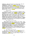 Table 30. Source of input values for parameters used to estimate kingfisher exposure.
Parameter
Body weight
Water intake
Food ingestion
Sediment ingestion
Proportion of diet • fish
Proportion of diet » invertebrates
Proportion of diet - amphibians
Home range
Variable
BW
IRW
IRFW
Value
0.147
0.11
0.5
PF
PI
PA
HR
0.46
0.24
0.27
0.39
Units
kg/bw
L/kg-bw/day
kg-food-wet-wt/kg-bw/day
kg-fish/kg-food
kg-inv/kg-food
kg-amph/kg-food
km of shoreline
Source(EPA1993a)
p 2-176; ave of 3 means for adults
p 2-176; adult rate
P 2-176
Assumed no incidental sediment ingestion
other than sediment in drinking water
p 2rl77; first entry; sum of trout and non-
trout
p 2-177; first entry; sum of insects and
Crustacea
p2-177; first entry
p 2-178; non-breeding
image:
Table 30. Source of input values for parameters used to estimate kingfisher exposure.
Parameter
Body weight
Water intake
Food ingestion
Sediment ingestion
Proportion of diet • fish
Proportion of diet » invertebrates
Proportion of diet - amphibians
Home range
Variable
BW
IRW
IRFW
Value
0.147
0.11
0.5
PF
PI
PA
HR
0.46
0.24
0.27
0.39
Units
kg/bw
L/kg-bw/day
kg-food-wet-wt/kg-bw/day
kg-fish/kg-food
kg-inv/kg-food
kg-amph/kg-food
km of shoreline
Source(EPA1993a)
p 2-176; ave of 3 means for adults
p 2-176; adult rate
P 2-176
Assumed no incidental sediment ingestion
other than sediment in drinking water
p 2rl77; first entry; sum of trout and non-
trout
p 2-177; first entry; sum of insects and
Crustacea
p2-177; first entry
p 2-178; non-breeding
image:
 Table 31. Source
concentrations of
of wildlife toxicity data used to estimate doses, dietary concentrations, and drinking water
metals non-toxic to kingfisher and sandpiper (same value used except where indicated by KF and SP).
Hg
Cd
Se
Pb
Variable
NTOXdose
NTOXdiet
NTOXwater
NTOXdose
NTOXdiet
NTOXwater
NTOXdose
NTOXdiet
NTOXdose
NTOXdiet
NTOXwater
Value
0.032
0.05
IxlO'7
I.SxIO7
42
0.1
0.003
2.1
5
2.8
500
0.1
Units
mg-Hg/kg-bw/day
mg-Hg/kg-diet
mg-Hg/L
mg-Hg/L
mg-Cd/kg-bw/day
mg-Cd/kg-diet
mg-Cd/L
mg-Se/kg-bw/day
mg-Se/kg-bw/day
mg-Pb/kg-bw/day
mg-Pb/kg-diet
mg-Pb/L
Source
EPA 1993a, p 2-7; proposed avian NOAEL (note: a factor of 0.1 is
recommended for application to kingfisher).
Eisler 1987, Table 1 1, p 71; no effect value for birds ranges from 0.05 to <0.1.
KF: EPA I993a, p 2-8; proposed no effect value for kingfisher.
SP: EPA 1993a, p 2-8; proposed avian value.
Eisler 1985a, p 34; mallard dietary value of 200 mg-Cd/kg-diet considered
here to be a LOAEL (divided by 2 to estimate NOAEL). Converted to dose
(see text). No species extrapolation factor used.
Eisler 1985a, p 34; wildlife dietary levels .above this value should be viewed
with caution.
Eisler I985a, p iii; above this level, adverse effects are pronounced or
probable.
Eisler 1985b, p 39; 5 ppm NOAEL; no effect on mallard and progeny;
converted to dose (see text). No species extrapolation factor used.
Eisler I985b, p 29; birds are sensitive to Se in diet at concentrations above 6
ppm. 5ppm is a NOAEL for the mallard. No species extrapolation factor used.
Eisler 1988, Table 7, p 84; no effect on starlings, effects on other species above
this level of organolead. No species extrapolation factor used.
Eisler 1988, p86; precocial birds NOAEL (growth) at 500 mg/kg.
Eisler 1988, Table 7, p 83; NOAEL for egg production in turtle-dove. No
species extrapolation factor used.
image:
Table 31. Source
concentrations of
of wildlife toxicity data used to estimate doses, dietary concentrations, and drinking water
metals non-toxic to kingfisher and sandpiper (same value used except where indicated by KF and SP).
Hg
Cd
Se
Pb
Variable
NTOXdose
NTOXdiet
NTOXwater
NTOXdose
NTOXdiet
NTOXwater
NTOXdose
NTOXdiet
NTOXdose
NTOXdiet
NTOXwater
Value
0.032
0.05
IxlO'7
I.SxIO7
42
0.1
0.003
2.1
5
2.8
500
0.1
Units
mg-Hg/kg-bw/day
mg-Hg/kg-diet
mg-Hg/L
mg-Hg/L
mg-Cd/kg-bw/day
mg-Cd/kg-diet
mg-Cd/L
mg-Se/kg-bw/day
mg-Se/kg-bw/day
mg-Pb/kg-bw/day
mg-Pb/kg-diet
mg-Pb/L
Source
EPA 1993a, p 2-7; proposed avian NOAEL (note: a factor of 0.1 is
recommended for application to kingfisher).
Eisler 1987, Table 1 1, p 71; no effect value for birds ranges from 0.05 to <0.1.
KF: EPA I993a, p 2-8; proposed no effect value for kingfisher.
SP: EPA 1993a, p 2-8; proposed avian value.
Eisler 1985a, p 34; mallard dietary value of 200 mg-Cd/kg-diet considered
here to be a LOAEL (divided by 2 to estimate NOAEL). Converted to dose
(see text). No species extrapolation factor used.
Eisler 1985a, p 34; wildlife dietary levels .above this value should be viewed
with caution.
Eisler I985a, p iii; above this level, adverse effects are pronounced or
probable.
Eisler 1985b, p 39; 5 ppm NOAEL; no effect on mallard and progeny;
converted to dose (see text). No species extrapolation factor used.
Eisler I985b, p 29; birds are sensitive to Se in diet at concentrations above 6
ppm. 5ppm is a NOAEL for the mallard. No species extrapolation factor used.
Eisler 1988, Table 7, p 84; no effect on starlings, effects on other species above
this level of organolead. No species extrapolation factor used.
Eisler 1988, p86; precocial birds NOAEL (growth) at 500 mg/kg.
Eisler 1988, Table 7, p 83; NOAEL for egg production in turtle-dove. No
species extrapolation factor used.
image:
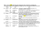 Table 32. Predicted toxicity or impoundment metals to the belted kingfisher (Ceryle alcyon). Calculated variables
are italicized. Sources of exposure and toxicity data are given in Tables 25 and 27-31.
EXPOSURE PARAMETERS:
KINGFISHER Units Variabli
Body weight = kg-bw BW
Digestion rale: water - L-water/kg-bw/day IRW
Ingestion rate: food (wet-wt)= kg-food-wet-wt/kg-bw/day ERFW
Proportion of diet that is Fish = kg-fish-wet-wl/kg-food-wet-wt PF
Proportion of diet that is Invertebrates = kg-inv-wet-wt/kg-food-wet-wt PI
Proportion of diet that is Amphibians = kg-amph-wet-wt/kg-food-wet-wt PA
Home range = km shoreline used HR
IMPOUNDMENT
Impoundment Shoreline:
Suspended Sediment:
km shoreline available
kg-sed-dry-wt/L
CONTAMINANT
Concentration in SEDIMENT = mg-cont/kg-sed-dry-wt
Concentration in WATER COL = mg-cont/L
BCF-water into fish = (mg-cont/kg-fish)/(mg-con(/L)
BCF-water into inverts = (mg-cont/kg-inv)/(mg-<x>nt/L)
BCF-water into amphibians = (mg-cont/kg-amphy(mg-<;ont/L)
SL
SS
CSED
CW
BCF-F
BCF-I
BCF-A
EXPOSURE CALCULATIONS:
VIA DIET
Concentration in Fish: CW*BCF-F=
Concentration in Invertebrates: CW*BCF-I=
Concentration in Amphibians: CW*BCF-A=
Dose from Fish: CF • IRFW*PF =
Dose from Benthic Inverts: CBI • IRFW*PI =
Dose from Amphibs: CA * IRFW*PA =
(mg-cont)/kg fish (wet wt)
(mg-cont)/kg inv (wet wt)
(mg-contykg amphibs (wet wt)
(mg-conty(kg-bwyday
(mg-contV(kg-bwyday
(mg-conty(kg-bwyday
VIA DRINKING WA TER
Dose from Water: CW*IRW = (mg-conty(kg-bwyday
Dose from Sed in Water: SS*IRW*CSED = (mg-conty(kg-bwyday
CF
a
CA
'DP
DI
DA
DW
DSW
Value
0.147
0.11
0.5
0.46
0.24
0.27
0.39
4
0.000385
CONTAMINANT
Hg
0.27
2.25E-05
95,000
95,000
95,000
2.14
2.14
2.14
0.492
0.257
0.289
2.48E-06
1.14E-05
Cd
11
4.50E-05
1500
1200
1500
0.0675
0.054
0.0675
0.0155
0.006
0.0091
4.95E-06
4.66E-04
Se
1
7.20E-05
1000
322
1000
0.072
0.023
0.072
0.0166
0.003
0.010
7.92R-06
4.24E-05
Pb
200
8.3E-05
726
5000
726
0.060
0.415
0.060
0.014
0.050'
0.0081
9.13E-06
8.47E-03
image:
Table 32. Predicted toxicity or impoundment metals to the belted kingfisher (Ceryle alcyon). Calculated variables
are italicized. Sources of exposure and toxicity data are given in Tables 25 and 27-31.
EXPOSURE PARAMETERS:
KINGFISHER Units Variabli
Body weight = kg-bw BW
Digestion rale: water - L-water/kg-bw/day IRW
Ingestion rate: food (wet-wt)= kg-food-wet-wt/kg-bw/day ERFW
Proportion of diet that is Fish = kg-fish-wet-wl/kg-food-wet-wt PF
Proportion of diet that is Invertebrates = kg-inv-wet-wt/kg-food-wet-wt PI
Proportion of diet that is Amphibians = kg-amph-wet-wt/kg-food-wet-wt PA
Home range = km shoreline used HR
IMPOUNDMENT
Impoundment Shoreline:
Suspended Sediment:
km shoreline available
kg-sed-dry-wt/L
CONTAMINANT
Concentration in SEDIMENT = mg-cont/kg-sed-dry-wt
Concentration in WATER COL = mg-cont/L
BCF-water into fish = (mg-cont/kg-fish)/(mg-con(/L)
BCF-water into inverts = (mg-cont/kg-inv)/(mg-<x>nt/L)
BCF-water into amphibians = (mg-cont/kg-amphy(mg-<;ont/L)
SL
SS
CSED
CW
BCF-F
BCF-I
BCF-A
EXPOSURE CALCULATIONS:
VIA DIET
Concentration in Fish: CW*BCF-F=
Concentration in Invertebrates: CW*BCF-I=
Concentration in Amphibians: CW*BCF-A=
Dose from Fish: CF • IRFW*PF =
Dose from Benthic Inverts: CBI • IRFW*PI =
Dose from Amphibs: CA * IRFW*PA =
(mg-cont)/kg fish (wet wt)
(mg-cont)/kg inv (wet wt)
(mg-contykg amphibs (wet wt)
(mg-conty(kg-bwyday
(mg-contV(kg-bwyday
(mg-conty(kg-bwyday
VIA DRINKING WA TER
Dose from Water: CW*IRW = (mg-conty(kg-bwyday
Dose from Sed in Water: SS*IRW*CSED = (mg-conty(kg-bwyday
CF
a
CA
'DP
DI
DA
DW
DSW
Value
0.147
0.11
0.5
0.46
0.24
0.27
0.39
4
0.000385
CONTAMINANT
Hg
0.27
2.25E-05
95,000
95,000
95,000
2.14
2.14
2.14
0.492
0.257
0.289
2.48E-06
1.14E-05
Cd
11
4.50E-05
1500
1200
1500
0.0675
0.054
0.0675
0.0155
0.006
0.0091
4.95E-06
4.66E-04
Se
1
7.20E-05
1000
322
1000
0.072
0.023
0.072
0.0166
0.003
0.010
7.92R-06
4.24E-05
Pb
200
8.3E-05
726
5000
726
0.060
0.415
0.060
0.014
0.050'
0.0081
9.13E-06
8.47E-03
image:
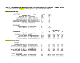 Table 32 (continued). Predicted toxicity of impoundment metals to the belted kingfisher.
CONTAMINANT
SUM ACROSS PA THWA YS
DF + DI + DA + DW + DSW= (mg-cont)/(kg-bwyday
CF*PF + CI*PI + CA'PA = (mg-conty(kg-diet)
CW= (mg-cont)/L
ADJUSTMENT FOR HOME RANGE
Home Range adjustment (if > 1 ) = HR7SL
TOXICITY PARAMETERS:
Dose Non-Toxic (o kingfisher = (mg-conty(kg-bw/day)
Diet Non-Toxic to kingfisher = (mg-cont)/kg-diet
Water Column cone non-toxic to kingfisher = (mg-cont)/L
HAZARD INDEX CALCULATION:
Exposure/Toxicity = EXP/(NTOXdose)
Or = EXPdietWTOXdiet
Or = nXPwater/NTOX water
EXPilose
EXPdiet
EXPwaler 1
IIRA
NTOXdose
NTOXdiet
NTOXwater
llldose
Uldiet
Illn-ater
IF BENTHIC INVERTEBRATES EXPOSED TO PORE WATER CONCENTRATIONS
Concentration in PORE water = ing-cont/L
EXPOSURE VIA DIET
Concentration in Benthic Invertebrates. CPW*BCF-1= (mg-cont)/kg inv (wet wt)
Dose from Denthic Inverts: CIPW * IRFW*PI = (mg-coniy(kg-bwyday
SUM A CROSS PA THWA YS
DF + DI + DA + DW + DSW= (mg-contV(kg-bwyday
CF'PF + Cl'Pt + CA*PA = (mg-conty(kg-diet)
HAZARD INDEX CALCULA T1ON:
Exposure/Toxicity = EXP/(NTOXdose)
Or = EXPdietMTOXdiet
CPW
cww
DIPW
EXPdose
EXPdiet
llldose
Uldiet
Hg
1.04
2.07
Cd
0.032
0.062
25E^)5 4.5E-05
-
0.032
0.050
1E-07
Hg
32
41
225
ARE
Hg
0.005
475
57
57.8
116
Hg
1806
2311
-
42
0.1
0.003
Cd
0.0
0.6
0.0
Se
0029
0.058
72E-05
—
2.1
5
—
Se
0.0
0.0
~~
Pb
0.080
0.144
8.3E-05
—
28
500
0.10
Pb
0.0
0.0
0.0
CONSUMED:
Cd
001
12
1.44
1.47
2.93
Cd
0.0
2?
Se
0016
5.15
0.618
0.645
1.29
Se
0.3
0.3
Pb
0.02
100
12
12.0
24.0
Pb
4.3
0.0
image:
Table 32 (continued). Predicted toxicity of impoundment metals to the belted kingfisher.
CONTAMINANT
SUM ACROSS PA THWA YS
DF + DI + DA + DW + DSW= (mg-cont)/(kg-bwyday
CF*PF + CI*PI + CA'PA = (mg-conty(kg-diet)
CW= (mg-cont)/L
ADJUSTMENT FOR HOME RANGE
Home Range adjustment (if > 1 ) = HR7SL
TOXICITY PARAMETERS:
Dose Non-Toxic (o kingfisher = (mg-conty(kg-bw/day)
Diet Non-Toxic to kingfisher = (mg-cont)/kg-diet
Water Column cone non-toxic to kingfisher = (mg-cont)/L
HAZARD INDEX CALCULATION:
Exposure/Toxicity = EXP/(NTOXdose)
Or = EXPdietWTOXdiet
Or = nXPwater/NTOX water
EXPilose
EXPdiet
EXPwaler 1
IIRA
NTOXdose
NTOXdiet
NTOXwater
llldose
Uldiet
Illn-ater
IF BENTHIC INVERTEBRATES EXPOSED TO PORE WATER CONCENTRATIONS
Concentration in PORE water = ing-cont/L
EXPOSURE VIA DIET
Concentration in Benthic Invertebrates. CPW*BCF-1= (mg-cont)/kg inv (wet wt)
Dose from Denthic Inverts: CIPW * IRFW*PI = (mg-coniy(kg-bwyday
SUM A CROSS PA THWA YS
DF + DI + DA + DW + DSW= (mg-contV(kg-bwyday
CF'PF + Cl'Pt + CA*PA = (mg-conty(kg-diet)
HAZARD INDEX CALCULA T1ON:
Exposure/Toxicity = EXP/(NTOXdose)
Or = EXPdietMTOXdiet
CPW
cww
DIPW
EXPdose
EXPdiet
llldose
Uldiet
Hg
1.04
2.07
Cd
0.032
0.062
25E^)5 4.5E-05
-
0.032
0.050
1E-07
Hg
32
41
225
ARE
Hg
0.005
475
57
57.8
116
Hg
1806
2311
-
42
0.1
0.003
Cd
0.0
0.6
0.0
Se
0029
0.058
72E-05
—
2.1
5
—
Se
0.0
0.0
~~
Pb
0.080
0.144
8.3E-05
—
28
500
0.10
Pb
0.0
0.0
0.0
CONSUMED:
Cd
001
12
1.44
1.47
2.93
Cd
0.0
2?
Se
0016
5.15
0.618
0.645
1.29
Se
0.3
0.3
Pb
0.02
100
12
12.0
24.0
Pb
4.3
0.0
image:
 Table 33. Estimating food ingestion rate for the sandpiper based on free-living metabolic rate and diet
of invertebrates; input values and method of calculation from EPA 1993 (see p4-17 for estimating ME).
Units
Variable
Value
1. Estimate Field Metabolic Rate Normalized to Body Weight
kcalAg-bw/day
NFMRkg
448
2. Normalize to Body Weight in g
NFMRkg* lkg/1000g =
kcal/g-bw/day
NI-MR
0.448
3. Estimate Average Metabolizable Energy
GE x AE = kcal-assim/g-inv-wet-wt
Dietary Item
Gross Energy
GE
kcal-gross/g-inv-we(-wt
ME
Assimil. Efficiency
AE
kcal-assim/kcal-gross
Invertebrates!
0.87
Metabolizable Energy
ME=GE x AE
kcal-assim/g-iliv-wel-wt
1
0.87
0.87
4. Estimate Total Normalized Ingestion Rate
NFMR/ME = g-inv-wet-wt/g-bw-day
IRFW
0.515
Source of Intuit Parameters (in EPA 1993)
NFMRkg p 2-152; average of means for adult free-living males and females.
GE p 4-1-3, Table 4-1; median number for invertebrates.
AE p 4-15, Table 4-3; assimilation efficiency of invertebrates.
image:
Table 33. Estimating food ingestion rate for the sandpiper based on free-living metabolic rate and diet
of invertebrates; input values and method of calculation from EPA 1993 (see p4-17 for estimating ME).
Units
Variable
Value
1. Estimate Field Metabolic Rate Normalized to Body Weight
kcalAg-bw/day
NFMRkg
448
2. Normalize to Body Weight in g
NFMRkg* lkg/1000g =
kcal/g-bw/day
NI-MR
0.448
3. Estimate Average Metabolizable Energy
GE x AE = kcal-assim/g-inv-wet-wt
Dietary Item
Gross Energy
GE
kcal-gross/g-inv-we(-wt
ME
Assimil. Efficiency
AE
kcal-assim/kcal-gross
Invertebrates!
0.87
Metabolizable Energy
ME=GE x AE
kcal-assim/g-iliv-wel-wt
1
0.87
0.87
4. Estimate Total Normalized Ingestion Rate
NFMR/ME = g-inv-wet-wt/g-bw-day
IRFW
0.515
Source of Intuit Parameters (in EPA 1993)
NFMRkg p 2-152; average of means for adult free-living males and females.
GE p 4-1-3, Table 4-1; median number for invertebrates.
AE p 4-15, Table 4-3; assimilation efficiency of invertebrates.
image:
 Table 34. Source of input values for parameters used to estimate sandpiper exposure
Parameter Variable Value
Body weight BW
Water intake IRW
Food ingestion IRFW
Units
0.0425 kg/bw
0.165 L/kg-bw/day
0.515
kg-food-wet-wt/
kg-bw/day
Source(EPA1993b; spotted sandpiper)
p 2-152; ave of means for adult males and females.
Ibid.
calculated in Table 31
Proportion of diet = sediment PDS
(dry wt)
Proportion of diet = PI
invertebrates
Home range HR
Proportion of invertebrates = PWI
water
0.18 kg-sed-dry-wt/
kg-(sed+food)-dry~wt species).
p 4-20; value for western sandpiper (median of 4
1 kg-inv/kg-food
2.5 km of shoreline
0.78 (wet-wt - dry-wt)/
wet-wt
p 2-152; dietary composition.
p 2-152; territory of 0.25 hectares; assume shoreline
width of 1m, the HR «= (0,25)*(10,000m2)/lm = 2.5 km.
p 4-13; median of 5 values for invertebrates.
image:
Table 34. Source of input values for parameters used to estimate sandpiper exposure
Parameter Variable Value
Body weight BW
Water intake IRW
Food ingestion IRFW
Units
0.0425 kg/bw
0.165 L/kg-bw/day
0.515
kg-food-wet-wt/
kg-bw/day
Source(EPA1993b; spotted sandpiper)
p 2-152; ave of means for adult males and females.
Ibid.
calculated in Table 31
Proportion of diet = sediment PDS
(dry wt)
Proportion of diet = PI
invertebrates
Home range HR
Proportion of invertebrates = PWI
water
0.18 kg-sed-dry-wt/
kg-(sed+food)-dry~wt species).
p 4-20; value for western sandpiper (median of 4
1 kg-inv/kg-food
2.5 km of shoreline
0.78 (wet-wt - dry-wt)/
wet-wt
p 2-152; dietary composition.
p 2-152; territory of 0.25 hectares; assume shoreline
width of 1m, the HR «= (0,25)*(10,000m2)/lm = 2.5 km.
p 4-13; median of 5 values for invertebrates.
image:
 Table 35. Predicted toxicity of impoundment metals to the sandpiper (Actitis macularia). Sources of exposure and toxicity data
are given in Tables 25, 27-29, 31, 33, and 34. Calculated variables are italicized.
EXPOSURE PARAMETERS:
SANDPIPER Units
Body weight = kg-bw
Digestion rate: water = L-water/kg-bw/day
Ingestion rate: food (wet-wt) = kg-food-wet-wt/kg-bw/day
Proportion of diet that is Invertebrates = kg-inv/kg-food
Proportion of Invertebrates that is water = (wet-wt - dry-wty wet-wt
Proportion of diet that is sediment = kg-sed-dry-wtAg-{sed+food)-dry-wt
Home range = km shoreline
IMPOUNDMENT
Impoundment Shoreline = km shoreline
Suspended Sediment = kg sed/L
CONTAMINANT
Concentration in SEDIMENT = mg-cont/kg-sed
Concentration in WATER COL = mg-cont/L
BCF-water into inverts = (mg-cont/kg-inv)/(ing-cont/L)
Variable
BW
IRW
IRFW
PI
PWI
PDS
HR
Value
0.0425
0.165
0.515
1
0.78
018
2.5
SL
SS
4
0.000385
CONTAMINANT
CSED
CW
BCF-I
«g
0.27
2.25E-05
95,000
Cd
11
4.50E-05
1200
Se
1
7.20E-05
322
Pb
200
8.30E-05
5000
EXPOSURE CALCULATIONS:
SEDIMENT INGESTION
Proportion of diet in dry weight = (1-PWI) = kg-food-dry-wlAg-ftxxl-wet-wi [>DD
Ratio of sediment to food (dry-wt)= PDS/( 1 -PDS) = kg-sediment-dry-wt/kg-food-dry-wt STl-'Jty
Ratio of sediment to food (wet-wt)= STFdry *PDD = kg-sediment-dry-wt/kg-food-wet-wt STFwet
Ingestion rate: sediment = IRFW*STFwet = kg-sed-dry-wt/kg-bw/day I1LS
VIA DIET
Concentration in Invertebrates: CW*BCF-I= (mg-cont)/kg inv (wet wt) Cl
Dose from Benthic Lwerts: CI * IRFW = (mg-cont)/(kg-bwXday DI
Dose from Sediment: CSED'IRS = (mg-cont)/(kg-bw)/day OS
0.22
0.22
0.0483
00249
2.14
MO
0.00671
0.0540
0.0278
0274
0.0232
0.0119
0.0249
0.415
0.214
4.97
image:
Table 35. Predicted toxicity of impoundment metals to the sandpiper (Actitis macularia). Sources of exposure and toxicity data
are given in Tables 25, 27-29, 31, 33, and 34. Calculated variables are italicized.
EXPOSURE PARAMETERS:
SANDPIPER Units
Body weight = kg-bw
Digestion rate: water = L-water/kg-bw/day
Ingestion rate: food (wet-wt) = kg-food-wet-wt/kg-bw/day
Proportion of diet that is Invertebrates = kg-inv/kg-food
Proportion of Invertebrates that is water = (wet-wt - dry-wty wet-wt
Proportion of diet that is sediment = kg-sed-dry-wtAg-{sed+food)-dry-wt
Home range = km shoreline
IMPOUNDMENT
Impoundment Shoreline = km shoreline
Suspended Sediment = kg sed/L
CONTAMINANT
Concentration in SEDIMENT = mg-cont/kg-sed
Concentration in WATER COL = mg-cont/L
BCF-water into inverts = (mg-cont/kg-inv)/(ing-cont/L)
Variable
BW
IRW
IRFW
PI
PWI
PDS
HR
Value
0.0425
0.165
0.515
1
0.78
018
2.5
SL
SS
4
0.000385
CONTAMINANT
CSED
CW
BCF-I
«g
0.27
2.25E-05
95,000
Cd
11
4.50E-05
1200
Se
1
7.20E-05
322
Pb
200
8.30E-05
5000
EXPOSURE CALCULATIONS:
SEDIMENT INGESTION
Proportion of diet in dry weight = (1-PWI) = kg-food-dry-wlAg-ftxxl-wet-wi [>DD
Ratio of sediment to food (dry-wt)= PDS/( 1 -PDS) = kg-sediment-dry-wt/kg-food-dry-wt STl-'Jty
Ratio of sediment to food (wet-wt)= STFdry *PDD = kg-sediment-dry-wt/kg-food-wet-wt STFwet
Ingestion rate: sediment = IRFW*STFwet = kg-sed-dry-wt/kg-bw/day I1LS
VIA DIET
Concentration in Invertebrates: CW*BCF-I= (mg-cont)/kg inv (wet wt) Cl
Dose from Benthic Lwerts: CI * IRFW = (mg-cont)/(kg-bwXday DI
Dose from Sediment: CSED'IRS = (mg-cont)/(kg-bw)/day OS
0.22
0.22
0.0483
00249
2.14
MO
0.00671
0.0540
0.0278
0274
0.0232
0.0119
0.0249
0.415
0.214
4.97
image:
 Table 35 (continued). Predicted toxicity of impoundment metals to the sandpiper.
VIA DRINKING WATER
Dose from Water: CW*IRW= (mg-cont)/(kg-bw)/day
Dose from Sed in Water: SS*IRW«CSFD = (mg-conty(kg-bwyday
SUM ACROSS PA THWA YS
DI + DS + DW + DSW = (mg-cont)/(kg-bw)/day
CI + STFwet'CSED = (mg-cont)/(kg-food)
CW= (mg-cont)/L
ADJUSTMENT FOR HOME RANGE:
Home Range adjustment (if > 1 ) - I IR/SL
TOXICITY PARAMETERS:
Dose Non-Toxic to sandpiper = (mg-cont)/(kg-bw/day)
Diet Non-Toxic to sandpiper * (mg-cont)/kg-diet
Water Column cone non-toxic to sandpiper = (mg-contyL
HAZARD INDEX CALCULATION:
Exposure/Toxicity = EXPdose/NTOXdose
Or = EXPdiet/NTOXdiet
Or = EXPwater/NTOX water
IF INVERTEBRATES EXPOSED TO PORE WATER ARE CONSUMED:
Concentration in PORE water = mg-cont/L
EXPOSURE VIA DIET
Concentration in Benthic Invertebrates: CPW*BCF-I= (mg-contykg inv (wet wt)
Dose from Benthic Inverts: CIPW* IRFW*PI = (mg-conty(kg-bwyday
SUM ACROSS PA THWA YS
DIPW + DS + DSW = (mg-conty(kg-bwyday
CIPW + STFwet'CSED = (mg-conty(kg-food)
HAZARD INDEX CALCULA TION:
Exposure/1 oxicity = EXP/(NTOXdose)
Or = EXPdiel/NTOXdiet
DW
DSW
EXPdose
EXPdiet
EXPwater
HRA
NTOXdose
NTOXdiet
NTOXwater
HIdose
Hldiet
lllwater
CPW
CIPW
DIPW
EXPdose
EXPdiet
Illdose
Hldiet
3.71E-06
1.72E-05
1.11
2.15
2.25E-05
-
0.032
0.05
1.80E-07
Hg
35
43
125
0.005
475
245
245
475
"g
7644
9500
7.43E-Q6
6.99E-04
0.302
0.585
4.50E-05
.
42
0.1
0.003
Cd
0.0
5.9
0.0
0.01
12.0
6.18
6.45
12.5
Cd
0.2
125
1.19E-05
6.35E-05
0.0369
0.0715
7.20E-05
-
21
5
Se
0.0
0.0
0.016
5.15
2.65
2.68
5.20
Se
1.3
1.0
1.37E-05
0.0127
5.20
10.1
8.30E-05
-
2.8
500
0.01
Pb
1.9
0.0
0.0
0.02
100
51.5
56.5
110
Pb
20
0
image:
Table 35 (continued). Predicted toxicity of impoundment metals to the sandpiper.
VIA DRINKING WATER
Dose from Water: CW*IRW= (mg-cont)/(kg-bw)/day
Dose from Sed in Water: SS*IRW«CSFD = (mg-conty(kg-bwyday
SUM ACROSS PA THWA YS
DI + DS + DW + DSW = (mg-cont)/(kg-bw)/day
CI + STFwet'CSED = (mg-cont)/(kg-food)
CW= (mg-cont)/L
ADJUSTMENT FOR HOME RANGE:
Home Range adjustment (if > 1 ) - I IR/SL
TOXICITY PARAMETERS:
Dose Non-Toxic to sandpiper = (mg-cont)/(kg-bw/day)
Diet Non-Toxic to sandpiper * (mg-cont)/kg-diet
Water Column cone non-toxic to sandpiper = (mg-contyL
HAZARD INDEX CALCULATION:
Exposure/Toxicity = EXPdose/NTOXdose
Or = EXPdiet/NTOXdiet
Or = EXPwater/NTOX water
IF INVERTEBRATES EXPOSED TO PORE WATER ARE CONSUMED:
Concentration in PORE water = mg-cont/L
EXPOSURE VIA DIET
Concentration in Benthic Invertebrates: CPW*BCF-I= (mg-contykg inv (wet wt)
Dose from Benthic Inverts: CIPW* IRFW*PI = (mg-conty(kg-bwyday
SUM ACROSS PA THWA YS
DIPW + DS + DSW = (mg-conty(kg-bwyday
CIPW + STFwet'CSED = (mg-conty(kg-food)
HAZARD INDEX CALCULA TION:
Exposure/1 oxicity = EXP/(NTOXdose)
Or = EXPdiel/NTOXdiet
DW
DSW
EXPdose
EXPdiet
EXPwater
HRA
NTOXdose
NTOXdiet
NTOXwater
HIdose
Hldiet
lllwater
CPW
CIPW
DIPW
EXPdose
EXPdiet
Illdose
Hldiet
3.71E-06
1.72E-05
1.11
2.15
2.25E-05
-
0.032
0.05
1.80E-07
Hg
35
43
125
0.005
475
245
245
475
"g
7644
9500
7.43E-Q6
6.99E-04
0.302
0.585
4.50E-05
.
42
0.1
0.003
Cd
0.0
5.9
0.0
0.01
12.0
6.18
6.45
12.5
Cd
0.2
125
1.19E-05
6.35E-05
0.0369
0.0715
7.20E-05
-
21
5
Se
0.0
0.0
0.016
5.15
2.65
2.68
5.20
Se
1.3
1.0
1.37E-05
0.0127
5.20
10.1
8.30E-05
-
2.8
500
0.01
Pb
1.9
0.0
0.0
0.02
100
51.5
56.5
110
Pb
20
0
image:
 Table 36. Estimating food ingestion rate for the river otter based on free-living metabolic rate and dietary composition.
Input values and method of calculation from EPA 1993 (see p4-17 for estimating ME).
Units Variable Value
1. Estimate Field Metabolic Rate Normalized to Body Weight
kcal/kg-bw/day NFMRkg 180
2. Normalize to Body Weight in g
NFMRkg* lkg/1000g = kcal/g-bw/day NI-MR 0.18
3. Estimate Average Metabolizable Energy
Sum (P x AE )= kcal-assim/g-inv-wet-wt AveME 0.98
Dietary Item
Fish
Invertebrates
Amphibians
Proportion
of Diet
P
0.53
0.26
0.16
Cross Energy
GE
kcal-gross/g-inv-wet-wt
1.2
1
1.2
Assimil. Efficiency
AE
kcal-assim/kcal-gross
0.91
0.87
0.91
Metabolizable Energy
ME=GE x AE
kcal-assim/g-inv-wet-wt
1.09
0.87
1.09
Weighted ME
P xME
kcal-assim/g-inv-wet-wt
0.579
0.226
0.175
4. Estimate Total Normalized Ingestion Rate
NFMR/AveME= g-inv-wet-wt/g-bw-day IRFW 0.184
Source of Input Parameters (in EPA 1993)
NFMRkg p 2-264; means for free-living otters.
GE p 4-13, Table 4-1; median number for invertebrates.
AE P 4-15, Table 4-3; assimilation efficiency of invertebrates.
image:
Table 36. Estimating food ingestion rate for the river otter based on free-living metabolic rate and dietary composition.
Input values and method of calculation from EPA 1993 (see p4-17 for estimating ME).
Units Variable Value
1. Estimate Field Metabolic Rate Normalized to Body Weight
kcal/kg-bw/day NFMRkg 180
2. Normalize to Body Weight in g
NFMRkg* lkg/1000g = kcal/g-bw/day NI-MR 0.18
3. Estimate Average Metabolizable Energy
Sum (P x AE )= kcal-assim/g-inv-wet-wt AveME 0.98
Dietary Item
Fish
Invertebrates
Amphibians
Proportion
of Diet
P
0.53
0.26
0.16
Cross Energy
GE
kcal-gross/g-inv-wet-wt
1.2
1
1.2
Assimil. Efficiency
AE
kcal-assim/kcal-gross
0.91
0.87
0.91
Metabolizable Energy
ME=GE x AE
kcal-assim/g-inv-wet-wt
1.09
0.87
1.09
Weighted ME
P xME
kcal-assim/g-inv-wet-wt
0.579
0.226
0.175
4. Estimate Total Normalized Ingestion Rate
NFMR/AveME= g-inv-wet-wt/g-bw-day IRFW 0.184
Source of Input Parameters (in EPA 1993)
NFMRkg p 2-264; means for free-living otters.
GE p 4-13, Table 4-1; median number for invertebrates.
AE P 4-15, Table 4-3; assimilation efficiency of invertebrates.
image:
 Table 37. Source of input values for parameters used to estimate river otter exposure
Parameter Variable
Body weight BW
Ingestion rate: water IRW
Ingestion rate: food IRFW
Proportion of diet - sediment PDS
(dry wt)
Proportion of diet « fish
" = invertebrates
" = amphibians
Home range
Proportion of fish = water
" invertebrates « water
" amphibians •= water PWA
PF
PI
PA
HR
PWF
PWI
0.53
0.258
0.16
28
0.72
0.78
Value
10
0.081
0.184
0.094
0.53
0.258
0.16
28
Units
kg/bw
L/kg-bw/day
kg-food-wet-wt/
kg-bw/day
kg-sed-dry-wt/
kg-(sed+food)-dry-wt
kg-fish/kg-food
kg-inv/kg-food
kg-amph/kg-food
km of shoreline
Source(EPA1993b;rlver otter)
p 2-264; midpoint of range for adult males and females.
p 2-264; average of means for adult males and females.
calculated in Table 36.
(wet-wt - dry-wt)/
wet-wt
(wet-wt - dry-wt)/
wet-wt
0.85
p 4-20; value for raccoon.
p 2-266, assuming % vol=% wt; combining 3 entries.
p 2-266, " .
p 2-266, " .
p 2-266; midpoint of range (10-78 km) for adult and
young, male and female.
p 4-13; average of 2 entries for fish.
p 4-13; median of 5 values for invertebrates.
p 4-13; value for frogs and toads.
image:
Table 37. Source of input values for parameters used to estimate river otter exposure
Parameter Variable
Body weight BW
Ingestion rate: water IRW
Ingestion rate: food IRFW
Proportion of diet - sediment PDS
(dry wt)
Proportion of diet « fish
" = invertebrates
" = amphibians
Home range
Proportion of fish = water
" invertebrates « water
" amphibians •= water PWA
PF
PI
PA
HR
PWF
PWI
0.53
0.258
0.16
28
0.72
0.78
Value
10
0.081
0.184
0.094
0.53
0.258
0.16
28
Units
kg/bw
L/kg-bw/day
kg-food-wet-wt/
kg-bw/day
kg-sed-dry-wt/
kg-(sed+food)-dry-wt
kg-fish/kg-food
kg-inv/kg-food
kg-amph/kg-food
km of shoreline
Source(EPA1993b;rlver otter)
p 2-264; midpoint of range for adult males and females.
p 2-264; average of means for adult males and females.
calculated in Table 36.
(wet-wt - dry-wt)/
wet-wt
(wet-wt - dry-wt)/
wet-wt
0.85
p 4-20; value for raccoon.
p 2-266, assuming % vol=% wt; combining 3 entries.
p 2-266, " .
p 2-266, " .
p 2-266; midpoint of range (10-78 km) for adult and
young, male and female.
p 4-13; average of 2 entries for fish.
p 4-13; median of 5 values for invertebrates.
p 4-13; value for frogs and toads.
image:
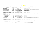 Table 38. Source
concentrations of
Hg
Variable
NTOXdose
NTOXdiet
NTOXwater
of wildlife toxicity data used
metals non-toxic to the river
Value Units
0.016 mg-Hg/kg-bw/day
1,1 mg-Hg/kg-diet
1.5x10* mg-Hg/L
to estimate doses, dietary concentrations, and drinking water
otter.
Source
EPA 1993a, p 2-2; proposed mammalian NOAEL.
Eisler 1987, Table II, p 71; no effect value for mammals.
EPA 1993a, p 2-3; proposed value for the otter.
Cd NTOXdose 0.9
NTOXdiet
NTOXwater
0.1
mg-Cd/kg-bw/day
mg-Cd/kg-diet
0.003 mg-Cd/L
Eisler 1985a, p 24; 1.8 ppm in oysters fed over 28 days to young mice is a
possible chronic LOAEL; factor of 2 used to extrapolate to NOAEL. No
species extrapolation factor used.
Eisler I985a, p 34; wildlife dietary levels above this value should be viewed
with caution.
Eisler 1985a, p Hi; above this level, adverse effects are pronounced or
probable.
Se NTOXdose 0.25
mg-Se/kg-bw/day
NTOXdiet
NTOXwater
mg-Se/kg-diet
0.05 mg-Se/L
Eisler 1985b, p 29; chronic selenosis in cattle at 0.5 mg-Se/kg-bw, possible
chronic LOAEL; lethal doses in other mammals occur above 1.5 mg-Se/kg-bw
(p 28); factor of 2 used to extrapolate to NOAEL. No species extrapolation
factor used.
Eisler 1985b, no dietary estimate considered protective of wildlife or mammals.
Eisler 1985b, p 41; 50 ppb is drinking water level protective of livestock. No
species extrapolation factor used.
Pb NTOXdose 0.05
NTOXdiet
NTOXwater
1.5
mg-Pb/kg-bw/day
mg-Pb/kg-diet
mg-Pb/L
Eisler 1988, Table 8, p 92; irreversible inhibition of ALAD activity in mouse at
0.05 mg-Pb/kg-bw/day; also, p 108, behavioral impairment in monkeys given
50 to 100 ug Pb/kg bw over 200 days. No species extrapolation factor used.
Eisler 1988, no dietary estimate considered protective of wildlife or mammals.
Eisler 1988, Table 8, pp. 92-97; wide range of no effects, from 20 to 2000
mg/L; effects in the rat as low as 1.5 mg/L (possible NOAEL). No species
extrapolation factor used.
image:
Table 38. Source
concentrations of
Hg
Variable
NTOXdose
NTOXdiet
NTOXwater
of wildlife toxicity data used
metals non-toxic to the river
Value Units
0.016 mg-Hg/kg-bw/day
1,1 mg-Hg/kg-diet
1.5x10* mg-Hg/L
to estimate doses, dietary concentrations, and drinking water
otter.
Source
EPA 1993a, p 2-2; proposed mammalian NOAEL.
Eisler 1987, Table II, p 71; no effect value for mammals.
EPA 1993a, p 2-3; proposed value for the otter.
Cd NTOXdose 0.9
NTOXdiet
NTOXwater
0.1
mg-Cd/kg-bw/day
mg-Cd/kg-diet
0.003 mg-Cd/L
Eisler 1985a, p 24; 1.8 ppm in oysters fed over 28 days to young mice is a
possible chronic LOAEL; factor of 2 used to extrapolate to NOAEL. No
species extrapolation factor used.
Eisler I985a, p 34; wildlife dietary levels above this value should be viewed
with caution.
Eisler 1985a, p Hi; above this level, adverse effects are pronounced or
probable.
Se NTOXdose 0.25
mg-Se/kg-bw/day
NTOXdiet
NTOXwater
mg-Se/kg-diet
0.05 mg-Se/L
Eisler 1985b, p 29; chronic selenosis in cattle at 0.5 mg-Se/kg-bw, possible
chronic LOAEL; lethal doses in other mammals occur above 1.5 mg-Se/kg-bw
(p 28); factor of 2 used to extrapolate to NOAEL. No species extrapolation
factor used.
Eisler 1985b, no dietary estimate considered protective of wildlife or mammals.
Eisler 1985b, p 41; 50 ppb is drinking water level protective of livestock. No
species extrapolation factor used.
Pb NTOXdose 0.05
NTOXdiet
NTOXwater
1.5
mg-Pb/kg-bw/day
mg-Pb/kg-diet
mg-Pb/L
Eisler 1988, Table 8, p 92; irreversible inhibition of ALAD activity in mouse at
0.05 mg-Pb/kg-bw/day; also, p 108, behavioral impairment in monkeys given
50 to 100 ug Pb/kg bw over 200 days. No species extrapolation factor used.
Eisler 1988, no dietary estimate considered protective of wildlife or mammals.
Eisler 1988, Table 8, pp. 92-97; wide range of no effects, from 20 to 2000
mg/L; effects in the rat as low as 1.5 mg/L (possible NOAEL). No species
extrapolation factor used.
image:
 Table 39. Predicted toxicity of impoundment metals to the river otter (Lutra canadensis). Calculated variables
are in italics. Sources of exposure and toxicity data are in Tables 25, 27-29, 36, and 37.
EXPOSURE PARAMETERS:
RIVER OTTER
Body weight =
Ingestion rate: water =
Ingestion rate: food (wet-wt) «
Proportion diet that is fish-
Proportion of diet that is invertebrates =
Proportion of diet that is amphibians =
Proportion of water in fish =
Proportion of water in invertebrates «
Proportion of water in amphibians =
Proportion of diet that is sediment =
Home range =
IMPOUNDMENT
Impoundment Shoreline:
Suspended Sediment •
CONTAMINANT
Concentration in SEDIMENT =
Concentration in PORE water =
Concentration in WATER COL =
BCF-water into fish =
BCF-water into inverts =
BCF-water into amphibians =
Unlti
kg-bw
L-water/kg-bw/day
kg-food-wet-wt/kg-bw/day
kg-fish/kg-food
kg-invertebrates/kg-food
kg-amphibians/kg-food
(wet-wt - dry-wtywet-wt
(wet-wt - dry-wtywet-wt
(wet-wt - dry-wtywet-wt
kg-sed-dry-wt/kg-{sed+food)-dry-wt
km shoreline
km shoreline
kgsed/L
mg-conl/kg-sed
mg-cont/L
mg-cont/L
(mg-cont/kg-fishy(mg-cont/L)
(mg-cont/kg-invy(mg-cont/L)
(mg-cont/kg-amphy(mg-cont/I,)
SL
SS
CSED
CPW
CW
BCF-F
BCF-I
BCF-A
Value
10.0000
0.081
0.184
0.53
0.26
016
0.72
078
085
0.094
28
4
0.000385
«g
0.27
0.005
2.25E-05
95000
95000
95000
CONTAMINANT
Cd Se Pb
11 1 200
0.01 0.016 0.02
4.50E-05 7.20E-05 8.30E-05
1500 1000 726
1200 322 5000
1500 1000 726
image:
Table 39. Predicted toxicity of impoundment metals to the river otter (Lutra canadensis). Calculated variables
are in italics. Sources of exposure and toxicity data are in Tables 25, 27-29, 36, and 37.
EXPOSURE PARAMETERS:
RIVER OTTER
Body weight =
Ingestion rate: water =
Ingestion rate: food (wet-wt) «
Proportion diet that is fish-
Proportion of diet that is invertebrates =
Proportion of diet that is amphibians =
Proportion of water in fish =
Proportion of water in invertebrates «
Proportion of water in amphibians =
Proportion of diet that is sediment =
Home range =
IMPOUNDMENT
Impoundment Shoreline:
Suspended Sediment •
CONTAMINANT
Concentration in SEDIMENT =
Concentration in PORE water =
Concentration in WATER COL =
BCF-water into fish =
BCF-water into inverts =
BCF-water into amphibians =
Unlti
kg-bw
L-water/kg-bw/day
kg-food-wet-wt/kg-bw/day
kg-fish/kg-food
kg-invertebrates/kg-food
kg-amphibians/kg-food
(wet-wt - dry-wtywet-wt
(wet-wt - dry-wtywet-wt
(wet-wt - dry-wtywet-wt
kg-sed-dry-wt/kg-{sed+food)-dry-wt
km shoreline
km shoreline
kgsed/L
mg-conl/kg-sed
mg-cont/L
mg-cont/L
(mg-cont/kg-fishy(mg-cont/L)
(mg-cont/kg-invy(mg-cont/L)
(mg-cont/kg-amphy(mg-cont/I,)
SL
SS
CSED
CPW
CW
BCF-F
BCF-I
BCF-A
Value
10.0000
0.081
0.184
0.53
0.26
016
0.72
078
085
0.094
28
4
0.000385
«g
0.27
0.005
2.25E-05
95000
95000
95000
CONTAMINANT
Cd Se Pb
11 1 200
0.01 0.016 0.02
4.50E-05 7.20E-05 8.30E-05
1500 1000 726
1200 322 5000
1500 1000 726
image:
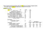 Table 39 (continued). Predicted toxicity of impoundment metals to the river otter
EXPOSURE CALCULATIONS:
SEDIMENT INGESTION
Proportion of diet which is dry weight = kg-food-dry-wt/kg-food-wet-wt
(1-PWF)«PF + (1-PWI)»P1 + (1-PWA)«PA
Ratio of sediment to food (dry-wt)= PDS/( 1 -PDS) = kg-sediment-dry-wt/kg-food-dry-wt
Ratio of sediment to food (wet-wt)= STFdry*PDD = kg-sediment-dry-wt/kg-food-wet-wt
Ingestion rate: sediment = IRFW*STFwet = kg-sed-dry-wtAg-food-dry-wt
PDD
VIA DIET
Concentration in Fish: CW*BCF-F=
Concentration in Invertebrates: CPW*BCF-I=
Concentration in Amphibians: CW*BCF-A=
Dose from Fish: CF * IRFW'PF =
Dose from Inverts. CI * IRFW*PI =
Dose from Amphibs: CA * IRFW*PA =
Dose from Sediment: CSED'IRS =
(mg-contykg fish (wet wt)
(mg-contykg inv (wet wt)
(mg-cont)/kg amph (wet wt)
(mg-conty(kg-bwyday
(mg-conty(kg-bwyday
(mg-conty(kg-bwyday
(mg-conty(kg-bwyday
0.23
STFdry
STFwet
IRS
0.10
0.0238
0.0044
CONTAMINANT
CF
CI
CA
DF
Dl
DA
DS
Hg
2.14
475
2.14
0.208
22.7
0.0628
0.00118
Cd
0.0675
12
0.0675
0.00657
0.573
0.00198
0.0481
Sc
0.0720
5.15
0.0720
0.00701
0.246
0.00212
0.00438
Pb
0.0603
100
0.0603
0.00587
4.78
0.00177
0.875
VIA DRINKING WATER
Dose from Water: CW*IRW= (mg-conty(kg-bwyday
Dojse from Sed in Water: SS*IRW*CSED = (mg-conty(kg-bwyday
SUM A CROSS PA THWA YS
DF + Dl + DA + DS + DW + DSW = (mg-conty(kg-bwyday
CF + CI + CA + STFwet'CSED = (mg-conty(kg-food)
CW= (mg-contyL
ADJUSTMENT FOR HOME RANGE:
Home Range adjustment (if >1) =
HR/SL
DW
DSW
liXPdose
EXPdiet
EXPwater
I1RA
1.82E-06
8.42E-06
23.0
479
225E-05
3.65E-06
3.43E-04
0.63
12.4
4.50E-05
5.83E-06
3.12E-05
0.26
5.32
7.20E-05
6.72E-06
0.0062
5.7
105
8.30E-05
image:
Table 39 (continued). Predicted toxicity of impoundment metals to the river otter
EXPOSURE CALCULATIONS:
SEDIMENT INGESTION
Proportion of diet which is dry weight = kg-food-dry-wt/kg-food-wet-wt
(1-PWF)«PF + (1-PWI)»P1 + (1-PWA)«PA
Ratio of sediment to food (dry-wt)= PDS/( 1 -PDS) = kg-sediment-dry-wt/kg-food-dry-wt
Ratio of sediment to food (wet-wt)= STFdry*PDD = kg-sediment-dry-wt/kg-food-wet-wt
Ingestion rate: sediment = IRFW*STFwet = kg-sed-dry-wtAg-food-dry-wt
PDD
VIA DIET
Concentration in Fish: CW*BCF-F=
Concentration in Invertebrates: CPW*BCF-I=
Concentration in Amphibians: CW*BCF-A=
Dose from Fish: CF * IRFW'PF =
Dose from Inverts. CI * IRFW*PI =
Dose from Amphibs: CA * IRFW*PA =
Dose from Sediment: CSED'IRS =
(mg-contykg fish (wet wt)
(mg-contykg inv (wet wt)
(mg-cont)/kg amph (wet wt)
(mg-conty(kg-bwyday
(mg-conty(kg-bwyday
(mg-conty(kg-bwyday
(mg-conty(kg-bwyday
0.23
STFdry
STFwet
IRS
0.10
0.0238
0.0044
CONTAMINANT
CF
CI
CA
DF
Dl
DA
DS
Hg
2.14
475
2.14
0.208
22.7
0.0628
0.00118
Cd
0.0675
12
0.0675
0.00657
0.573
0.00198
0.0481
Sc
0.0720
5.15
0.0720
0.00701
0.246
0.00212
0.00438
Pb
0.0603
100
0.0603
0.00587
4.78
0.00177
0.875
VIA DRINKING WATER
Dose from Water: CW*IRW= (mg-conty(kg-bwyday
Dojse from Sed in Water: SS*IRW*CSED = (mg-conty(kg-bwyday
SUM A CROSS PA THWA YS
DF + Dl + DA + DS + DW + DSW = (mg-conty(kg-bwyday
CF + CI + CA + STFwet'CSED = (mg-conty(kg-food)
CW= (mg-contyL
ADJUSTMENT FOR HOME RANGE:
Home Range adjustment (if >1) =
HR/SL
DW
DSW
liXPdose
EXPdiet
EXPwater
I1RA
1.82E-06
8.42E-06
23.0
479
225E-05
3.65E-06
3.43E-04
0.63
12.4
4.50E-05
5.83E-06
3.12E-05
0.26
5.32
7.20E-05
6.72E-06
0.0062
5.7
105
8.30E-05
image:
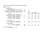 Table 39 (continued). Predicted toxicity of impoundment metals to the river otter
CONTAMINANT
TOXICITY PARAMETERS:
Dose Non-Toxic to river otter = (mg-conty(kg-bw/day)
Diet Non-Toxic to river otter = (mg-cont)/kg-diet
Water Column cone non-toxic to river otter = (mg-cont)/I-
HAZARD INDEX CALCULATION:
Exposure/Toxicity = EXPdose/NTOXdose/HRA
Or =EXPdiet/NTOXdiet/IIRA
Or = EXPwater/NTOXwater/HRA
IF 50% OF INVERTEBRATES CONSUMED ARE EXPOSED TO PORE WATER:
EXPOSURE VIA DIET
Concentration in Invertebrates (ave): = (mg-cont)/kg inv (wet wt)
0.5*(CPW+CW)*BCF-I=
Dose from Denthic Inverts: CIPW* IRFW'PI = (mg-cont)/(kg-bw)/day
SUM ACROSS PA THWA YS
DF + DIPW + DA + DS + DW + DSW = (mg-conl)/(kg-bw)/day
CF + CIPW + CA + STFwet'CSED = (mg-cont)/(kg-food)
HAZARD INDEX CALCULA TION:
Exposure/Toxicity = EXP/(NTOXdose)/I IRA
Or = EXPdiel/NTOXdiet/HRA
NTOXdose
NTOXdiet
NTOXwater
Illdose
Illdiet
Hlwater
CIPW
•
DIPW
EXPdose
EXPdiet
Illdose
Hldiei
Hg
0.016
1.1
1.50E-06
Hg
205
62
2
239
11.4
11.7
243
Hg
104
32
Cd
0.9
0.1
0.003
Cd
0.1
18
0.0
6.03
0.288
0.345
6.42
Cd
0.1
9.2
Se
0.25
-
0.05
Se
0.1
-
0.0
2.59
0.124
0.137
2.76
Se
0.1
-
Pb
0.05
-
1.50
Pb
16.2
-
0.0
50.2
2.40
3.29
55.1
Pb
9.4
-
image:
Table 39 (continued). Predicted toxicity of impoundment metals to the river otter
CONTAMINANT
TOXICITY PARAMETERS:
Dose Non-Toxic to river otter = (mg-conty(kg-bw/day)
Diet Non-Toxic to river otter = (mg-cont)/kg-diet
Water Column cone non-toxic to river otter = (mg-cont)/I-
HAZARD INDEX CALCULATION:
Exposure/Toxicity = EXPdose/NTOXdose/HRA
Or =EXPdiet/NTOXdiet/IIRA
Or = EXPwater/NTOXwater/HRA
IF 50% OF INVERTEBRATES CONSUMED ARE EXPOSED TO PORE WATER:
EXPOSURE VIA DIET
Concentration in Invertebrates (ave): = (mg-cont)/kg inv (wet wt)
0.5*(CPW+CW)*BCF-I=
Dose from Denthic Inverts: CIPW* IRFW'PI = (mg-cont)/(kg-bw)/day
SUM ACROSS PA THWA YS
DF + DIPW + DA + DS + DW + DSW = (mg-conl)/(kg-bw)/day
CF + CIPW + CA + STFwet'CSED = (mg-cont)/(kg-food)
HAZARD INDEX CALCULA TION:
Exposure/Toxicity = EXP/(NTOXdose)/I IRA
Or = EXPdiel/NTOXdiet/HRA
NTOXdose
NTOXdiet
NTOXwater
Illdose
Illdiet
Hlwater
CIPW
•
DIPW
EXPdose
EXPdiet
Illdose
Hldiei
Hg
0.016
1.1
1.50E-06
Hg
205
62
2
239
11.4
11.7
243
Hg
104
32
Cd
0.9
0.1
0.003
Cd
0.1
18
0.0
6.03
0.288
0.345
6.42
Cd
0.1
9.2
Se
0.25
-
0.05
Se
0.1
-
0.0
2.59
0.124
0.137
2.76
Se
0.1
-
Pb
0.05
-
1.50
Pb
16.2
-
0.0
50.2
2.40
3.29
55.1
Pb
9.4
-
image:
 The field metabolic rate (NFMRkg, in kcal/kg-bw/day, which •
is the metabolic need of the otter, taken from EPA [1993b],
p2-264, the mean for free-living otters) was normalized to a
per gram body weight (kcal/g-bw/day) . This was divided by
the average kcal available in the diet (MEavg, in kcal/g-
diet-wet-wt) and the result expressed as kg-food-wet-wt/kg-
bw/day. Proportions of dietary components, gross energy of
each component (GE) and assimilation efficiency (AE) of each
component were used to calculate the average kcal in the
diet. The proportions of diet that are fish (PF) ,
invertebrates (PI), and amphibians (PA) were based on
percentages taken from EPA (1993b; also see Table 35, here).
The gross energy (GE) and assimilation efficiencies (AE)
were taken from EPA (1993) Figure 4-7, and Table 4-1 (median
value for invertebrates was used for GE) .
The ingested dose of contaminants in food was estimated by
first calculating the dose from each food component. In general,
three components were evaluated, fish, invertebrates, and
amphibians. As mentioned just above, the proportions of each of
these in the diet were obtained. The proportions were multiplied
by the ingestion rate to get component-specific ingestion rates
which were then multiplied by the contaminant concentration in
the component. This tissue concentration was estimated by
multiplying the appropriate medium concentration by a
bioaccumulation factor. For example, for an organism exposed to
mercury (see Table 37), the dose from fish (DF; mg-Hg/kg-bw/day)
is given by: •
(1) DF = CF * IRFW * PF
where:
CF is the concentration in fish (mg-Hg/kg-fish-wet-wt)
IRFW is the food ingestion rate (kg-food-wet-wt/kg-bw/day)
PF is the proportion of food that is fish
(kg-fish-wet-wt/kg-food-wet-wt)
And CF is given by:
(2) CF = CW * BCF-F
where:
CW is the concentration in water (mg-Hg/L)
BCF-F is the bioconcentration factor for water into fish
([mg-Hg/kg-fish-wet-wt]/[mg-Hg/L])
Using these parameters and equations, contaminant doses were
estimated for each category then summed, along with sediment
ingestion and drinking water doses.
155
image:
The field metabolic rate (NFMRkg, in kcal/kg-bw/day, which •
is the metabolic need of the otter, taken from EPA [1993b],
p2-264, the mean for free-living otters) was normalized to a
per gram body weight (kcal/g-bw/day) . This was divided by
the average kcal available in the diet (MEavg, in kcal/g-
diet-wet-wt) and the result expressed as kg-food-wet-wt/kg-
bw/day. Proportions of dietary components, gross energy of
each component (GE) and assimilation efficiency (AE) of each
component were used to calculate the average kcal in the
diet. The proportions of diet that are fish (PF) ,
invertebrates (PI), and amphibians (PA) were based on
percentages taken from EPA (1993b; also see Table 35, here).
The gross energy (GE) and assimilation efficiencies (AE)
were taken from EPA (1993) Figure 4-7, and Table 4-1 (median
value for invertebrates was used for GE) .
The ingested dose of contaminants in food was estimated by
first calculating the dose from each food component. In general,
three components were evaluated, fish, invertebrates, and
amphibians. As mentioned just above, the proportions of each of
these in the diet were obtained. The proportions were multiplied
by the ingestion rate to get component-specific ingestion rates
which were then multiplied by the contaminant concentration in
the component. This tissue concentration was estimated by
multiplying the appropriate medium concentration by a
bioaccumulation factor. For example, for an organism exposed to
mercury (see Table 37), the dose from fish (DF; mg-Hg/kg-bw/day)
is given by: •
(1) DF = CF * IRFW * PF
where:
CF is the concentration in fish (mg-Hg/kg-fish-wet-wt)
IRFW is the food ingestion rate (kg-food-wet-wt/kg-bw/day)
PF is the proportion of food that is fish
(kg-fish-wet-wt/kg-food-wet-wt)
And CF is given by:
(2) CF = CW * BCF-F
where:
CW is the concentration in water (mg-Hg/L)
BCF-F is the bioconcentration factor for water into fish
([mg-Hg/kg-fish-wet-wt]/[mg-Hg/L])
Using these parameters and equations, contaminant doses were
estimated for each category then summed, along with sediment
ingestion and drinking water doses.
155
image:
 Bioconcentration factors for mercury, cadmium, selenium, and
lead are shown in Table 29.
iii. Sediment Ingestion Rate and Dose.
Estimates of the sediment ingestion rates (IRS; kg-sed-dry-
wt/kg-bw/day) were calculated as follows (refer also to Tables 35
and 39):
(1) IRS = IRFW * STFwet
where:
IRFW is the food ingestion rate (kg-food-wet-wt/kg-bw/day),
and is obtained as described previously.
STFwet is the ratio of sediment to food in the diet on a wet
weight basis (kg-sed-dry-wt/kg-food-wet-wt).
And, since
(2) STFwet = STFdry * FDD
where:
STFdry is the ratio of sediment to food in the diet on a dry
weight basis (kg-sed-dry-wt/kg-food-dry-wt).
FDD converts from wet weight to dry weight (kg-food-dry-
wt/kg-food-wet-wt)
STFdry and FDD are obtained as follows:
(3) STFdry = PDS/(1-PDS)
where:
PDS is the proportion of total ingested material that is
sediment on a dry weight basis (kg-sed-dry-wt/kg-
food+sediment-dry-wt) and is obtained from EPA (1993b)
listings of percent sediment in diet. For example, a PDS of
0.094 was chosen for the otter (EPA [1993b] p 4-20, using
the value listed for the raccoon).
and:
(4) FDD = (1-PWF)*(PF) + (1-PWI)*(PI) + (1-PWA)*(PA)
where:
FDD converts ingestion rates from wet to dry weight (kg-
food-dry-wt/kg-food-wet-wt).
156
image:
Bioconcentration factors for mercury, cadmium, selenium, and
lead are shown in Table 29.
iii. Sediment Ingestion Rate and Dose.
Estimates of the sediment ingestion rates (IRS; kg-sed-dry-
wt/kg-bw/day) were calculated as follows (refer also to Tables 35
and 39):
(1) IRS = IRFW * STFwet
where:
IRFW is the food ingestion rate (kg-food-wet-wt/kg-bw/day),
and is obtained as described previously.
STFwet is the ratio of sediment to food in the diet on a wet
weight basis (kg-sed-dry-wt/kg-food-wet-wt).
And, since
(2) STFwet = STFdry * FDD
where:
STFdry is the ratio of sediment to food in the diet on a dry
weight basis (kg-sed-dry-wt/kg-food-dry-wt).
FDD converts from wet weight to dry weight (kg-food-dry-
wt/kg-food-wet-wt)
STFdry and FDD are obtained as follows:
(3) STFdry = PDS/(1-PDS)
where:
PDS is the proportion of total ingested material that is
sediment on a dry weight basis (kg-sed-dry-wt/kg-
food+sediment-dry-wt) and is obtained from EPA (1993b)
listings of percent sediment in diet. For example, a PDS of
0.094 was chosen for the otter (EPA [1993b] p 4-20, using
the value listed for the raccoon).
and:
(4) FDD = (1-PWF)*(PF) + (1-PWI)*(PI) + (1-PWA)*(PA)
where:
FDD converts ingestion rates from wet to dry weight (kg-
food-dry-wt/kg-food-wet-wt).
156
image:
 PWF, PWI, .and PWA are the proportions of fish,
invertebrates, and amphibians that are water (kg-water/kg-
food; or [kg-food-wet-wt - kg-food-dry-wt]/kg-food-wet-wt).
PF, PI, and PA are the proportions of the diet that are
fish, invertebrates, and amphibians.
PDD was estimated from data in Table 4-1 of EPA (1993b) as
follows: 0.72 (mean of two values) was used as the proportion of
fish that is water (PWF); 0.78 (the median of five values, after
computing the midpoints of ranges) was used as the proportion of
invertebrates that is water (PWI); and 0.85 (single value) was
used for amphibians (PWA). These proportions were converted to
proportion dry matter by subtracting from 1, yielding units of
dry-wt/wet-wt. These new proportions (dry-wt/wet-wt) were then
multiplied by the proportion of that dietary item in the total
diet to convert ingestion rates to a dry weight basis.
For example, the river otter ingests 0.184 kg-food-wet-
wt/kg-bw/day, 0.53 of which is fish (PF) at 72% water (PWF), 0.26
of which is invertebrates (PI) .at 78% water, and 0.16 of which is
amphibians. (PA) at 85% water. Therefore, PDD would be:
0.53 kg-fish-wet-wt/kg-food-wet-wt x
(100-72)%, or 0.28 kg-fish-dry-wt/kg-fish-wet-wt
plus
0.26 kg-inv-wet-wt/kg-food-wet-wt x
0.22 kg-inv-dry-wt/kg-inv-wet-wt
plus
0.16 kg-amph-wet-wt/kg-food-wet-wt x
0.15 kg-amph-dry-wt/kg-amph-wet-wt
which totals to 0.23 kg-food-dry-wt/kg-food-wet-wt.
The dose (mg-sed associated contaminant/kg bwt/day) was
calculated by multiplying the ingestion rate (IRS) by the
contaminant concentration in the sediment.
b. Comparisons between exposure and toxicity.
Three approaches were used. First, the doses were summed
(food, water, sediment in drinking water, other incidental
sediment ingestion) to produce a total dose (mg-contaminant/kg-
body weight/day) and this was compared with literature toxicity
data. The assumption made here was that all of the contaminant
ingested would be at least as bioavailable as the form of the
contaminant used in the toxicity studies. The main comparison of
interest was to compare the ingested dose with a NOAEL (no
adverse effects level) dose. In general, NOAELs were obtained
from the literature or else doses characterized as non-toxic to
wildlife were used. Similarly, dietary concentrations
characterized as non-toxic to wildlife of some general subgoup of
157
image:
PWF, PWI, .and PWA are the proportions of fish,
invertebrates, and amphibians that are water (kg-water/kg-
food; or [kg-food-wet-wt - kg-food-dry-wt]/kg-food-wet-wt).
PF, PI, and PA are the proportions of the diet that are
fish, invertebrates, and amphibians.
PDD was estimated from data in Table 4-1 of EPA (1993b) as
follows: 0.72 (mean of two values) was used as the proportion of
fish that is water (PWF); 0.78 (the median of five values, after
computing the midpoints of ranges) was used as the proportion of
invertebrates that is water (PWI); and 0.85 (single value) was
used for amphibians (PWA). These proportions were converted to
proportion dry matter by subtracting from 1, yielding units of
dry-wt/wet-wt. These new proportions (dry-wt/wet-wt) were then
multiplied by the proportion of that dietary item in the total
diet to convert ingestion rates to a dry weight basis.
For example, the river otter ingests 0.184 kg-food-wet-
wt/kg-bw/day, 0.53 of which is fish (PF) at 72% water (PWF), 0.26
of which is invertebrates (PI) .at 78% water, and 0.16 of which is
amphibians. (PA) at 85% water. Therefore, PDD would be:
0.53 kg-fish-wet-wt/kg-food-wet-wt x
(100-72)%, or 0.28 kg-fish-dry-wt/kg-fish-wet-wt
plus
0.26 kg-inv-wet-wt/kg-food-wet-wt x
0.22 kg-inv-dry-wt/kg-inv-wet-wt
plus
0.16 kg-amph-wet-wt/kg-food-wet-wt x
0.15 kg-amph-dry-wt/kg-amph-wet-wt
which totals to 0.23 kg-food-dry-wt/kg-food-wet-wt.
The dose (mg-sed associated contaminant/kg bwt/day) was
calculated by multiplying the ingestion rate (IRS) by the
contaminant concentration in the sediment.
b. Comparisons between exposure and toxicity.
Three approaches were used. First, the doses were summed
(food, water, sediment in drinking water, other incidental
sediment ingestion) to produce a total dose (mg-contaminant/kg-
body weight/day) and this was compared with literature toxicity
data. The assumption made here was that all of the contaminant
ingested would be at least as bioavailable as the form of the
contaminant used in the toxicity studies. The main comparison of
interest was to compare the ingested dose with a NOAEL (no
adverse effects level) dose. In general, NOAELs were obtained
from the literature or else doses characterized as non-toxic to
wildlife were used. Similarly, dietary concentrations
characterized as non-toxic to wildlife of some general subgoup of
157
image:
 interest (such .as birds) were also used. Dietary concentrations
for individual species (e.g., mallard) were not used, because
scaling from that species to the species of interest (e.g.,
kingfisher) involved computing the dose first. There was no need
to derive a dietary concentration if a suitable dose was
available.
If no suitable dose was available, however, it was estimated
from dietary exposure if the dietary concentration was available.
For example, given a dietary NOAEL concentration of 100 mg-Cd/kg-
food or 5 mg-Se/kg-food for the mallard, the NOAEL can be
multiplied by the mallard ingestion rate to yield a daily
acceptable dose. The mallard ingestion rate can be derived from
the mallard body weight of 1225 g (EPA I993b, p2-43) using
equation 3-5 of EPA (1993b; p3-5) which expresses ingestion as g-
food-dry-wt/day using the formula:
food ingestion (g-food-dry-wt/day) = 0.495 Body wt (g) * 0.704
This ingestion rate can then be converted to a wet-weight basis
by multiplying by 7 g-food-wet-wt/g-food-dry-wt (Eisler reports
conversion factors of 4 and 10 in 1985b, p 37 and 1988 p 71,
respectively). Based on the example presented above, mallard
food intake is calculated to be 73.9 g-food-dry-wt/day, which
converts to 0.517 kg-food-wet-wt/day. This can be scaled to body
weight to yield 0.42 kd-food-wet-wt/kg-bw/day. Multiplying this
by the non-toxic NOAELs of 100 mg-Cd/kg-food and 5 mg-Se/kg-food
yields 42 mg-Cd/kg-bw/day and 2.1 mg-Se/kg-bw-day.
Second, an attempt was made to estimate the dietary exposure
in terms of mg-contaminant/kg-diet and compare this exposure with
toxicity data similarly expressed. This was done by multiplying
tissue concentrations for fish, amphibians, and invertebrates by
their relative percent contributions to the diet, then summing.
To this sum was added an estimate of the dietary contribution by
incidental sediment ingestion. This component was estimated by
multiplying STFwet (the ratio of sediment-dry-weight to food-
wet-weight) by sediment contaminant concentrations. For example,
for the river otter ingesting mercury:
STFwet = 0.0218 kg-sed-dry-wt/kg-food-wet-wt
And, multiplying by the mercury concentration of 0.27 mg-cont/kg-
sed-dry-wt, yields:
0.0059 mg-Hg/kg-food-wet-wt (incidental sediment ingestion)
Note how this adds only a small amount to the total dietary
concentration of mercury intake which is estimated at 33.3 mg-
Hg/kg-food-wet-wt (Table 39, EXPdiet).
158
image:
interest (such .as birds) were also used. Dietary concentrations
for individual species (e.g., mallard) were not used, because
scaling from that species to the species of interest (e.g.,
kingfisher) involved computing the dose first. There was no need
to derive a dietary concentration if a suitable dose was
available.
If no suitable dose was available, however, it was estimated
from dietary exposure if the dietary concentration was available.
For example, given a dietary NOAEL concentration of 100 mg-Cd/kg-
food or 5 mg-Se/kg-food for the mallard, the NOAEL can be
multiplied by the mallard ingestion rate to yield a daily
acceptable dose. The mallard ingestion rate can be derived from
the mallard body weight of 1225 g (EPA I993b, p2-43) using
equation 3-5 of EPA (1993b; p3-5) which expresses ingestion as g-
food-dry-wt/day using the formula:
food ingestion (g-food-dry-wt/day) = 0.495 Body wt (g) * 0.704
This ingestion rate can then be converted to a wet-weight basis
by multiplying by 7 g-food-wet-wt/g-food-dry-wt (Eisler reports
conversion factors of 4 and 10 in 1985b, p 37 and 1988 p 71,
respectively). Based on the example presented above, mallard
food intake is calculated to be 73.9 g-food-dry-wt/day, which
converts to 0.517 kg-food-wet-wt/day. This can be scaled to body
weight to yield 0.42 kd-food-wet-wt/kg-bw/day. Multiplying this
by the non-toxic NOAELs of 100 mg-Cd/kg-food and 5 mg-Se/kg-food
yields 42 mg-Cd/kg-bw/day and 2.1 mg-Se/kg-bw-day.
Second, an attempt was made to estimate the dietary exposure
in terms of mg-contaminant/kg-diet and compare this exposure with
toxicity data similarly expressed. This was done by multiplying
tissue concentrations for fish, amphibians, and invertebrates by
their relative percent contributions to the diet, then summing.
To this sum was added an estimate of the dietary contribution by
incidental sediment ingestion. This component was estimated by
multiplying STFwet (the ratio of sediment-dry-weight to food-
wet-weight) by sediment contaminant concentrations. For example,
for the river otter ingesting mercury:
STFwet = 0.0218 kg-sed-dry-wt/kg-food-wet-wt
And, multiplying by the mercury concentration of 0.27 mg-cont/kg-
sed-dry-wt, yields:
0.0059 mg-Hg/kg-food-wet-wt (incidental sediment ingestion)
Note how this adds only a small amount to the total dietary
concentration of mercury intake which is estimated at 33.3 mg-
Hg/kg-food-wet-wt (Table 39, EXPdiet).
158
image:
 Third, where possible, water column concentrations were
compared with proposed water quality criteria protective of
wildlife. These three comparisons were also adjusted for the
influence of home range relative to the size of the impoundment
(assumed to have a shoreline length of 4 km).
5^ Kingfisher - Exposure, Toxicity, and Effects
The sources of the input values used to estimate kingfisher
exposure are shown in Table 30. Based on the reported density of
0.15 to 0.6 pairs of kingfishers per km of shoreline (EPA 1993b,
p 2-178) , the proposed impoundment could support a pair. The
sources of the toxicity data selected to evaluate potential
effects to kingfishers that might utilize the impoundment are
presented in Table 31.
Results of exposure and toxicity calculations for the
kingfisher are shown in Table 32. Cadmium is not expected-to
present a problem to kingfishers. However, mercury in particular
as well as lead and selenium may be at concentrations above a
level of no effect. Although bioavailability of these metals may
be overestimated for ingestion of sediments in drinking-water,
this component has only a minor contribution. In addition, if
species extrapolation factors are used, the hazard indices would
increase by an order of magnitude.
6^_ Exposure and Toxicity to the Sandpiper
The sources of the input values used to estimate sandpiper
exposure are shown in Tables 32 and 33. Based on the reported
density of about 12 per hectare in summer (EPA 1993b, p 2-153)
and assuming a shoreline width of 1 m, the proposed impoundment
(4 km of shoreline) could support approximately 5 birds (i.e.,
[4 000 m shoreline length x 1 m width] x [0.0001 hectare/in x 12
birds/hectare] =4.8 birds). The sources of the toxicity data
selected to evaluate potential effects to sandpipers that might
utilize the impoundment are presented in Table 31.
Results of exposure and toxicity calculations for the
sandpiper are shown in Table 35. Based on the assumptions and
values used selenium is not expected to be present in
concentrations toxic to sandpipers. Mercury in particular may be
at concentrations above a level of no effect as might cadmium and
lead to a lesser extent. Based on comparisons of pathways,
most of the exposure to mercury comes from ingestion of
invertebrates, whereas the pathway of concern for lead and
cadmium is sediment ingestion (estimated separately from
159
image:
Third, where possible, water column concentrations were
compared with proposed water quality criteria protective of
wildlife. These three comparisons were also adjusted for the
influence of home range relative to the size of the impoundment
(assumed to have a shoreline length of 4 km).
5^ Kingfisher - Exposure, Toxicity, and Effects
The sources of the input values used to estimate kingfisher
exposure are shown in Table 30. Based on the reported density of
0.15 to 0.6 pairs of kingfishers per km of shoreline (EPA 1993b,
p 2-178) , the proposed impoundment could support a pair. The
sources of the toxicity data selected to evaluate potential
effects to kingfishers that might utilize the impoundment are
presented in Table 31.
Results of exposure and toxicity calculations for the
kingfisher are shown in Table 32. Cadmium is not expected-to
present a problem to kingfishers. However, mercury in particular
as well as lead and selenium may be at concentrations above a
level of no effect. Although bioavailability of these metals may
be overestimated for ingestion of sediments in drinking-water,
this component has only a minor contribution. In addition, if
species extrapolation factors are used, the hazard indices would
increase by an order of magnitude.
6^_ Exposure and Toxicity to the Sandpiper
The sources of the input values used to estimate sandpiper
exposure are shown in Tables 32 and 33. Based on the reported
density of about 12 per hectare in summer (EPA 1993b, p 2-153)
and assuming a shoreline width of 1 m, the proposed impoundment
(4 km of shoreline) could support approximately 5 birds (i.e.,
[4 000 m shoreline length x 1 m width] x [0.0001 hectare/in x 12
birds/hectare] =4.8 birds). The sources of the toxicity data
selected to evaluate potential effects to sandpipers that might
utilize the impoundment are presented in Table 31.
Results of exposure and toxicity calculations for the
sandpiper are shown in Table 35. Based on the assumptions and
values used selenium is not expected to be present in
concentrations toxic to sandpipers. Mercury in particular may be
at concentrations above a level of no effect as might cadmium and
lead to a lesser extent. Based on comparisons of pathways,
most of the exposure to mercury comes from ingestion of
invertebrates, whereas the pathway of concern for lead and
cadmium is sediment ingestion (estimated separately from
159
image:
 total ingested .close. A second, more conservative scenario where •
the invertebrate prey are exposed to pore water concentrations,
suggests that all of the metals would be of concern, particularly
mercury, followed by cadmium and lead. It is important to note
that if species extrapolation factors are used, the hazard
indices would increase by an order of magnitude.
7. Exposure and Toxicity to the River Otter
The sources of the input values used to estimate river otter
exposure are shown in Tables 38 and 39. Based on the reported
density of about one otter per 28 km of shoreline (EPA 1993b, p
2-266), the proposed impoundment (4 km of shoreline) could be
important in supporting an otter. The sources of the toxicity
data selected to evaluate potential effects to river otters that
might utilize the impoundment are presented in Table 38.
Results of exposure and toxicity calculations for the river
otter are shown in Table 39. Based on the assumptions and values
used and adjusting for home range, selenium is not expected to be
present in toxic concentrations.. Mercury in particular may be at
concentrations above a level of no effect as might cadmium and
lead to a lesser extent. As was found in the analyses for the
two bird species, ingestion of water and sediments in drinking
water are likely to be minor contributions to the total ingested
dose. A second, less conservative scenario where half rather
than all the invertebrate prey are exposed to pore water
concentrations, does not change the above results appreciably.
Based on comparisons of pathways, most of the exposure to
the metals comes from ingestion of invertebrates with additional
doses contributed from fish or sediment ingestion depending on
the metal. As pointed out for the bird species, it is important
to note again that if species extrapolation factors are used, the
hazard indices would increase by an order of magnitude.
K._ Uncertainty Factors
This analysis builds on data supplied from other sections of
this report and so incorporates the uncertainties in those
sections by reference. For the most part, sediment, pore water,
and water column toxicity were evaluated by comparison with
benchmarks, and the uncertainties in each of those benchmarks
(water quality criteria and sediment benchmarks) are similarly
incorporated by reference. However, the analysis of potential
toxicity to wildlife has several types of uncertainty that can
only be reduced with further site-specific exposure and toxicity
information.
Several assumptions were made concerning exposure of the
selected species. The animals are expected to ingest resuspended
sediments along with their drinking water, and these sediments
160
image:
total ingested .close. A second, more conservative scenario where •
the invertebrate prey are exposed to pore water concentrations,
suggests that all of the metals would be of concern, particularly
mercury, followed by cadmium and lead. It is important to note
that if species extrapolation factors are used, the hazard
indices would increase by an order of magnitude.
7. Exposure and Toxicity to the River Otter
The sources of the input values used to estimate river otter
exposure are shown in Tables 38 and 39. Based on the reported
density of about one otter per 28 km of shoreline (EPA 1993b, p
2-266), the proposed impoundment (4 km of shoreline) could be
important in supporting an otter. The sources of the toxicity
data selected to evaluate potential effects to river otters that
might utilize the impoundment are presented in Table 38.
Results of exposure and toxicity calculations for the river
otter are shown in Table 39. Based on the assumptions and values
used and adjusting for home range, selenium is not expected to be
present in toxic concentrations.. Mercury in particular may be at
concentrations above a level of no effect as might cadmium and
lead to a lesser extent. As was found in the analyses for the
two bird species, ingestion of water and sediments in drinking
water are likely to be minor contributions to the total ingested
dose. A second, less conservative scenario where half rather
than all the invertebrate prey are exposed to pore water
concentrations, does not change the above results appreciably.
Based on comparisons of pathways, most of the exposure to
the metals comes from ingestion of invertebrates with additional
doses contributed from fish or sediment ingestion depending on
the metal. As pointed out for the bird species, it is important
to note again that if species extrapolation factors are used, the
hazard indices would increase by an order of magnitude.
K._ Uncertainty Factors
This analysis builds on data supplied from other sections of
this report and so incorporates the uncertainties in those
sections by reference. For the most part, sediment, pore water,
and water column toxicity were evaluated by comparison with
benchmarks, and the uncertainties in each of those benchmarks
(water quality criteria and sediment benchmarks) are similarly
incorporated by reference. However, the analysis of potential
toxicity to wildlife has several types of uncertainty that can
only be reduced with further site-specific exposure and toxicity
information.
Several assumptions were made concerning exposure of the
selected species. The animals are expected to ingest resuspended
sediments along with their drinking water, and these sediments
160
image:
 are assumed to .come entirely from tailings. Resuspension of
tailings and .their subsequent settlement along the shoreline has
not been modeled, nor is it understood whether such a scenario
would result in elevated levels of metals in near-shore pore
water as compared to the water column. In general, it was
assumed that ingested metals were as bioavailable as the form of
the contaminants used in the toxicity tests that form the basis
for comparison. While this may be an overestimate for sediments,
tissue concentrations are likely to be highly bioavailable and
these doses seemed to contribute the most contaminants to the
overall dose.
Similarly, selecting from a range of available toxicity data
is not straightforward. Ideally, one would like to find several
studies that generate NOAEL's (no adverse affect levels) for dose
or dietary concentration that are based.on chronic studies using
endpoints that are relevant to populations or individuals of the
selected species. Because these data are generally not available
to this level of desired detail, selections are made and
extrapolation factors are used. Here, extrapolation factors were
used only to estimate a NOAEL f;rom a LOAEL (lowest adverse effect
level) , where a factor of two was used. It could be argued for
most of the wildlife comparisons that an additional factor of at
least 10 be used to reflect the uncertainty of applying data from
acute studies on species other than the one of concern.
Nevertheless, despite these and other sources of
uncertainty, the attempt here was made to select organisms that
could reasonably represent a range of wildlife that would use the
impoundment area. In addition, the following guidelines were
used to avoid creating an unrealistic or overconservative
analysis: (I) average wildlife exposure parameters were used (vs
selecting maximum ingestion rates, smallest body weights,
juveniles, etc.); (2) reasonable estimates were used for most
parameters. For example, BCFs were taken from those used in
other analyses of wildlife (EPA I993a), and where possible, non-
toxic doses and dietary concentrations were taken from Eisler's
summaries (1985a, 1985b, 1987); and (3) species sensitivity
factors were not used, but could be factored in. Also, the
sensitivity of the models used here were examined for the
response of the hazard indices to assumptions about the exposure
of invertebrates to pore water.
Based on the approach used here, the results are useful in:
(1) indicating the general expected toxicity of impoundment
sediments, pore water, and the potential for bioaccumulation; and
(2) describing the uncertainties of the proposed project in terms
of the potential of the impoundment to affect aquatic and benthic
biota as well as wildlife upon cessation of the discharge.
161
image:
are assumed to .come entirely from tailings. Resuspension of
tailings and .their subsequent settlement along the shoreline has
not been modeled, nor is it understood whether such a scenario
would result in elevated levels of metals in near-shore pore
water as compared to the water column. In general, it was
assumed that ingested metals were as bioavailable as the form of
the contaminants used in the toxicity tests that form the basis
for comparison. While this may be an overestimate for sediments,
tissue concentrations are likely to be highly bioavailable and
these doses seemed to contribute the most contaminants to the
overall dose.
Similarly, selecting from a range of available toxicity data
is not straightforward. Ideally, one would like to find several
studies that generate NOAEL's (no adverse affect levels) for dose
or dietary concentration that are based.on chronic studies using
endpoints that are relevant to populations or individuals of the
selected species. Because these data are generally not available
to this level of desired detail, selections are made and
extrapolation factors are used. Here, extrapolation factors were
used only to estimate a NOAEL f;rom a LOAEL (lowest adverse effect
level) , where a factor of two was used. It could be argued for
most of the wildlife comparisons that an additional factor of at
least 10 be used to reflect the uncertainty of applying data from
acute studies on species other than the one of concern.
Nevertheless, despite these and other sources of
uncertainty, the attempt here was made to select organisms that
could reasonably represent a range of wildlife that would use the
impoundment area. In addition, the following guidelines were
used to avoid creating an unrealistic or overconservative
analysis: (I) average wildlife exposure parameters were used (vs
selecting maximum ingestion rates, smallest body weights,
juveniles, etc.); (2) reasonable estimates were used for most
parameters. For example, BCFs were taken from those used in
other analyses of wildlife (EPA I993a), and where possible, non-
toxic doses and dietary concentrations were taken from Eisler's
summaries (1985a, 1985b, 1987); and (3) species sensitivity
factors were not used, but could be factored in. Also, the
sensitivity of the models used here were examined for the
response of the hazard indices to assumptions about the exposure
of invertebrates to pore water.
Based on the approach used here, the results are useful in:
(1) indicating the general expected toxicity of impoundment
sediments, pore water, and the potential for bioaccumulation; and
(2) describing the uncertainties of the proposed project in terms
of the potential of the impoundment to affect aquatic and benthic
biota as well as wildlife upon cessation of the discharge.
161
image:
 L^. SUMMARY OF- EXCEEDANCES OF CRITERIA AND BENCHMARKS
PORE WATER (Tables 25 and 26)
Exceedance of AWQC
- Acute:
CU (12X), Hg (2x), NH3 (5x) , Cr (2x)*, CN (200x)**
- Chronic:Cd (2x), Se (3x)
*If Cr(VI); **CN criterion applied to CNfree
Exceedance of aquatic values of concern
- High end of concentration range:CNS (16x)
- Low end of concentration range: CNO (4x), Xanthate (93x)
SEDIMENT (Table 27)
Exceedance of Provincial Sediment Quality Guidelines
- Severe Effect:Cd (lx), Cu (2x), Fe (lx), Mn (4x)
- Lowest Effect:
Ag (6x), As (2x), Cr (lx), Hg (lx), Ni (2x), Pb (7x), Zn
(4X), CNtot (420X)
Exceedance of Wisconsin DNR Guidelines:
Cd (llx), Cu (3x), Hg (3x), Pb (4x) , Zn (5x), As & Se (lx)
Exceedance of Draft Great Lakes ERMs:
Cd (3x), Cu (lx), Pb (2x)
WATER COLUMN (Table 28)
Exceedance of AWQC
- Acute:Cu (2x)
- Chronic:Hg (60x)
WILDLIFE (Cd, Pb, Hg, Se) (Tables 32, 35, and 39)
Exceedance of estimated nontoxic dose:
Kingfisher:Hg (32x)
Sandpiper:Hg (35x), Pb (2x)
River Otter:Hg (205x), Pb (16x)
Exceedance of estimated nontoxic dietary concentration:
Kingfisher:Hg (41x)
Sandpiper:Hg (43x), Cd (6x)
162
image:
L^. SUMMARY OF- EXCEEDANCES OF CRITERIA AND BENCHMARKS
PORE WATER (Tables 25 and 26)
Exceedance of AWQC
- Acute:
CU (12X), Hg (2x), NH3 (5x) , Cr (2x)*, CN (200x)**
- Chronic:Cd (2x), Se (3x)
*If Cr(VI); **CN criterion applied to CNfree
Exceedance of aquatic values of concern
- High end of concentration range:CNS (16x)
- Low end of concentration range: CNO (4x), Xanthate (93x)
SEDIMENT (Table 27)
Exceedance of Provincial Sediment Quality Guidelines
- Severe Effect:Cd (lx), Cu (2x), Fe (lx), Mn (4x)
- Lowest Effect:
Ag (6x), As (2x), Cr (lx), Hg (lx), Ni (2x), Pb (7x), Zn
(4X), CNtot (420X)
Exceedance of Wisconsin DNR Guidelines:
Cd (llx), Cu (3x), Hg (3x), Pb (4x) , Zn (5x), As & Se (lx)
Exceedance of Draft Great Lakes ERMs:
Cd (3x), Cu (lx), Pb (2x)
WATER COLUMN (Table 28)
Exceedance of AWQC
- Acute:Cu (2x)
- Chronic:Hg (60x)
WILDLIFE (Cd, Pb, Hg, Se) (Tables 32, 35, and 39)
Exceedance of estimated nontoxic dose:
Kingfisher:Hg (32x)
Sandpiper:Hg (35x), Pb (2x)
River Otter:Hg (205x), Pb (16x)
Exceedance of estimated nontoxic dietary concentration:
Kingfisher:Hg (41x)
Sandpiper:Hg (43x), Cd (6x)
162
image:
 River-Otter:Hg (62x), Cd (18x) (NA for Se, Pb)
Exceedance of draft Great Lakes Water criterion for Hg:
Kingfisher:Yes 225 x
Sandpiper:Yes 125 x
River Otter:Yes 2 x
If benthic invertebrates are exposed to pore water and are then
consumed, the following additional contaminants are of concern to
the kingfisher and sandpiper:
Exceedance of estimated nontoxic dose:
Kingfisher:Pb (4x)
Sandpiper:Se (Ix)
Exceedance of estimated nontoxic dietary concentration:
Kingfisher:Cd (29x)
Sandpiper:Se (Ix)
M.. Review of Literature on Subaqueous Disposal of Mine Tailings
The Mine Environment Neutral Drainage (MEND) studies,
conducted by a consortium of Canadian government agencies and
industry representatives, examined lakes in Canada that have been
used in the past for subaqueous disposal of mine taili-ngs. Four
potentially relevant Canadian lakes studied included Buttle Lake,
Anderson Lake, Mandy Lake and Benson Lake, with results presented
in a number of reports. These studies are of some use in
predicting what could occur in the AJ tailings impoundment in
terms of uptake of metals, and were subsequently reviewed by the
Rawson Academy in terms of the utility of the subaqueous disposal
technique. A major difference between the lakes reviewed and the
proposed impoundment is that the lakes reviewed have very
different characteristics in terms of sediment inputs and
existing biological communities than might be expected in the
Sheep Creek tailings impoundment.
The Rawson Academy's review of the studies conducted on
three of these lakes (Buttle,. Anderson and Mandy) is summarized
in a report entitled A Critical Review of MEND Studies Conducted
to 1991 on Subaqueous Disposal of Tailings RAAS 7/92 SRT Report.
The review is not an endorsement of the disposal technique in all
cases. For example,
p 2 "The process of tailings disposal is potentially
highlv"disruptive of lake ecosystems and normally it would take
several decades (possibly centuries in some lakes) before natural
sedimentation provided sufficient cover to insulate the lake
ecosystem from the influence of the tailings (both the metals
flux and substrate effects)."
163
image:
River-Otter:Hg (62x), Cd (18x) (NA for Se, Pb)
Exceedance of draft Great Lakes Water criterion for Hg:
Kingfisher:Yes 225 x
Sandpiper:Yes 125 x
River Otter:Yes 2 x
If benthic invertebrates are exposed to pore water and are then
consumed, the following additional contaminants are of concern to
the kingfisher and sandpiper:
Exceedance of estimated nontoxic dose:
Kingfisher:Pb (4x)
Sandpiper:Se (Ix)
Exceedance of estimated nontoxic dietary concentration:
Kingfisher:Cd (29x)
Sandpiper:Se (Ix)
M.. Review of Literature on Subaqueous Disposal of Mine Tailings
The Mine Environment Neutral Drainage (MEND) studies,
conducted by a consortium of Canadian government agencies and
industry representatives, examined lakes in Canada that have been
used in the past for subaqueous disposal of mine taili-ngs. Four
potentially relevant Canadian lakes studied included Buttle Lake,
Anderson Lake, Mandy Lake and Benson Lake, with results presented
in a number of reports. These studies are of some use in
predicting what could occur in the AJ tailings impoundment in
terms of uptake of metals, and were subsequently reviewed by the
Rawson Academy in terms of the utility of the subaqueous disposal
technique. A major difference between the lakes reviewed and the
proposed impoundment is that the lakes reviewed have very
different characteristics in terms of sediment inputs and
existing biological communities than might be expected in the
Sheep Creek tailings impoundment.
The Rawson Academy's review of the studies conducted on
three of these lakes (Buttle,. Anderson and Mandy) is summarized
in a report entitled A Critical Review of MEND Studies Conducted
to 1991 on Subaqueous Disposal of Tailings RAAS 7/92 SRT Report.
The review is not an endorsement of the disposal technique in all
cases. For example,
p 2 "The process of tailings disposal is potentially
highlv"disruptive of lake ecosystems and normally it would take
several decades (possibly centuries in some lakes) before natural
sedimentation provided sufficient cover to insulate the lake
ecosystem from the influence of the tailings (both the metals
flux and substrate effects)."
163
image:
 p. 2. "The background limnologies of the MEND case study
lakes (Anderson, Buttle, Mandy) are suitable only for gross
comparisons. They do not support clear interpretation of cause
and effect associated with tailings disposal."
p. 3. "..the data are neither useful to address effects
which occur during the process of disposal nor long term
ecosystem adjustments to the introductions of tailings."
p. 9. Concerns to be addressed: Biological and physical
reworking of tailings underwater, burial of benthic biota (and
modification of food web structure), effects of solids ingestion
on metal uptake by organisms.
p. 10. "The application of a single "generic" approach to
subaqueous tailings disposal does not seem practical,
considerations ... should be site-specific."
p. 12. "..the background limnologies are inadequate to
establish anything other than the most obvious trends in lake
conditions."
Subsequent to the Rawson Academy review, the MEND program
conducted a preliminary biological and geological assessment of
Benson Lake. Of the lakes studied to date, the Benson Lake
setting appears to be most applicable to the AJ mine project with
some caveats. Benson Lake is described as a small, deep,
oligotrophic coastal mountain lake situated in the coastal
western hemlock biogeoclimatic zone on the northern end of
Vancouver Island. Benson Lake was used as a tailings repository
for approximately eleven years by the Benson Lake Coast Copper-
Mine operated by Cominco Ltd. Operations ceased in 1973. This
lake is not comparable in terms of some site specifics,
especially the fact that Benson Lake is an existing lake with
supporting aquatic and riparian habitats, populations, and
relatively large stream inflows allowing foraging and
recruitment. The regeneration of the communities associated with
this lake are not applicable to the AJ project.
Aquatic vegetation was well established in the littoral zone
of the lake and compared to a control lake, aquatic vegetation in
Benson Lake was found to contain elevated levels of arsenic and
copper. Arsenic accumulated in the tops and roots of horsetail
(Jfguisetum sp.) and pond weed (Potamogeton sp.) . The roots of
both species had very high levels of arsenic ranging from 100 to
320 ug/g and 330 to 2100 ug/g respectively. Copper accumulated
in the roots of horsetail and in the tops and roots of pond weed.
Spper in horsetail roots ranged from 29 ug/g to 380 ug/g. Roots
typically accumulated more metal than the tops (MEND, 1991).
Concentrations of metals in the flesh of fish from Benson
Lake were lower than for the control lake. However,
164
image:
p. 2. "The background limnologies of the MEND case study
lakes (Anderson, Buttle, Mandy) are suitable only for gross
comparisons. They do not support clear interpretation of cause
and effect associated with tailings disposal."
p. 3. "..the data are neither useful to address effects
which occur during the process of disposal nor long term
ecosystem adjustments to the introductions of tailings."
p. 9. Concerns to be addressed: Biological and physical
reworking of tailings underwater, burial of benthic biota (and
modification of food web structure), effects of solids ingestion
on metal uptake by organisms.
p. 10. "The application of a single "generic" approach to
subaqueous tailings disposal does not seem practical,
considerations ... should be site-specific."
p. 12. "..the background limnologies are inadequate to
establish anything other than the most obvious trends in lake
conditions."
Subsequent to the Rawson Academy review, the MEND program
conducted a preliminary biological and geological assessment of
Benson Lake. Of the lakes studied to date, the Benson Lake
setting appears to be most applicable to the AJ mine project with
some caveats. Benson Lake is described as a small, deep,
oligotrophic coastal mountain lake situated in the coastal
western hemlock biogeoclimatic zone on the northern end of
Vancouver Island. Benson Lake was used as a tailings repository
for approximately eleven years by the Benson Lake Coast Copper-
Mine operated by Cominco Ltd. Operations ceased in 1973. This
lake is not comparable in terms of some site specifics,
especially the fact that Benson Lake is an existing lake with
supporting aquatic and riparian habitats, populations, and
relatively large stream inflows allowing foraging and
recruitment. The regeneration of the communities associated with
this lake are not applicable to the AJ project.
Aquatic vegetation was well established in the littoral zone
of the lake and compared to a control lake, aquatic vegetation in
Benson Lake was found to contain elevated levels of arsenic and
copper. Arsenic accumulated in the tops and roots of horsetail
(Jfguisetum sp.) and pond weed (Potamogeton sp.) . The roots of
both species had very high levels of arsenic ranging from 100 to
320 ug/g and 330 to 2100 ug/g respectively. Copper accumulated
in the roots of horsetail and in the tops and roots of pond weed.
Spper in horsetail roots ranged from 29 ug/g to 380 ug/g. Roots
typically accumulated more metal than the tops (MEND, 1991).
Concentrations of metals in the flesh of fish from Benson
Lake were lower than for the control lake. However,
164
image:
 concentrations of arsenic, copper, cobalt, and cadmium were
significantly higher in the livers of fish from Benson Lake,
suggesting metals bioaccumulation.
These data indicate that metals have accumulated in
vegetation and fish from Benson Lake when compared to a control
lake.
N. Laboratory Tests Relevant to the Long-Term Behavior of
Metals and Other Constituents.
The ecological risk analysis presented earlier in this
chapter is based in part on analyses of the tailings. A
principal concern is the bioavailability of metals to organisms
that could inhabit the impoundment which is in utrn related to
the mobility of the metals.
Two types of information, leach tests and indicators of acid
generation potential, provide an empirical basis to evaluate the
mobility of metals from the solid phase into water (see Table 3).
As with samples discussed earlier for decant tests, a major
concern with analytical results for leach tests and acid
generation potential of tailings material has been a lack of
information on the representativeness of the materials tested
with respect to the material expected to come out of the mill.
As noted above, data intended to demonstrate the
representativeness of the average nature of bulk ore samples used
in test work have recently been provided by Echo Bay (EBA,
1994a,b). The availability of a single tailings sample, if
representative, provides at best average values for test results
rather than reasonable maximum values.
1. Leach Tests.
Column leach tests were conducted in 1989 (Ott, 1989) and
1991 (Andrews, 1991) on tailings material. Little information
has been available on the source of material and methods used in
the 1989 tests and they are not discussed further here. The 1991
column tests were done on tailings produced from a bulk sample of
ore collected from the 4387SX crosscut in the North Ore Body.
Tailings from this sample have undergone a variety of tests and
have been the primary focus of testing for the FEIS (Table 4).
The column tests which extended up to about 240 days
indicated an early release of many constituents, such as cyanide,
thought be be related to the tailings water. The results were
used in conjunction with decant data (both in the FEIS and in
this report in Table 5) to develop estimates of tailings water
composition for projections of pond pore-water quality. A
tabulation of column test and decant results is included Appendix
B (Tables B-l and B-2).
165
image:
concentrations of arsenic, copper, cobalt, and cadmium were
significantly higher in the livers of fish from Benson Lake,
suggesting metals bioaccumulation.
These data indicate that metals have accumulated in
vegetation and fish from Benson Lake when compared to a control
lake.
N. Laboratory Tests Relevant to the Long-Term Behavior of
Metals and Other Constituents.
The ecological risk analysis presented earlier in this
chapter is based in part on analyses of the tailings. A
principal concern is the bioavailability of metals to organisms
that could inhabit the impoundment which is in utrn related to
the mobility of the metals.
Two types of information, leach tests and indicators of acid
generation potential, provide an empirical basis to evaluate the
mobility of metals from the solid phase into water (see Table 3).
As with samples discussed earlier for decant tests, a major
concern with analytical results for leach tests and acid
generation potential of tailings material has been a lack of
information on the representativeness of the materials tested
with respect to the material expected to come out of the mill.
As noted above, data intended to demonstrate the
representativeness of the average nature of bulk ore samples used
in test work have recently been provided by Echo Bay (EBA,
1994a,b). The availability of a single tailings sample, if
representative, provides at best average values for test results
rather than reasonable maximum values.
1. Leach Tests.
Column leach tests were conducted in 1989 (Ott, 1989) and
1991 (Andrews, 1991) on tailings material. Little information
has been available on the source of material and methods used in
the 1989 tests and they are not discussed further here. The 1991
column tests were done on tailings produced from a bulk sample of
ore collected from the 4387SX crosscut in the North Ore Body.
Tailings from this sample have undergone a variety of tests and
have been the primary focus of testing for the FEIS (Table 4).
The column tests which extended up to about 240 days
indicated an early release of many constituents, such as cyanide,
thought be be related to the tailings water. The results were
used in conjunction with decant data (both in the FEIS and in
this report in Table 5) to develop estimates of tailings water
composition for projections of pond pore-water quality. A
tabulation of column test and decant results is included Appendix
B (Tables B-l and B-2).
165
image:
 Batch-type" leach tests (EP - extraction procedure toxicity
and TCLP - toxicity characteristic leaching procedure) of
tailings believed to have been previously leached in the 1991
columns (Table 4 and Bergstrom, 1993) were conducted to provide a
comparison with the hazardous waste toxicity characteristic under
the Resources Conservation and Recovery Act (RCRA). Because of
the previous column leaching, the batch tests are not useful for
hazardous waste characterization of the raw tailings.
Furthermore, the tests are not necessarily appropriate for
determining the mobility of contaminants from mine wastes under
environmental conditions at the tailings impoundment because of
the organic acid leachant and the limited analyte list.
2. Acid Generation Potential.
The oxidation of sulfur in the presence of water can produce
sulfuric acid which can in turn liberate metals at concentrations
well above what might be released under near-neutral pH
conditions. The presence of calcium carbonate and other alkaline
minerals, however, can neutralize acid if the minerals are
available in sufficient quantity and dispersed such that
neutralizing reactions-can occur at rates exceeding the acid
generating reactions. Two means of assessing the potential for
acid drainage from the mine workings, waste rock, and tailings
are available for the AJ project:
* Historical drainage characteristics from old mine workings
and tailings piles.
* Laboratory tests of acid generation potential of samples
from the mine sites.
Several historical mine workings and waste dumps occur near
Juneau (Bureau of Land Management, 1992). Reports of acid
drainage have not been found for these localities. However, the
use of new processing techniques and methods of waste disposal
for AJ would argue against reliance on historical information
alone as the sole basis for evaluating the potential for acid
generation.
The FEIS notes that Lakefield Research tests indicate
flotation tailings would have a net potential to consume acid,
and cyanided tailings might be acid producing. The FEIS
concludes that combined tailings are «... expected to provide a
relatively strong potential for acid consumption." (BLM, iyy^,
p 4-42) Actual data to support the FEIS statement were sparse
at best because of lack of information on the source and
variability of samples. Extensive additional data on sulfur
content and acid-base accounting tests for ore and waste rock
were provided in 1994 by Echo Bay (EBA, 1994b). These results
demonstrate that the sulfur content of ore and waste rock is
sufficiently low enough and the neutralization potential high
166
image:
Batch-type" leach tests (EP - extraction procedure toxicity
and TCLP - toxicity characteristic leaching procedure) of
tailings believed to have been previously leached in the 1991
columns (Table 4 and Bergstrom, 1993) were conducted to provide a
comparison with the hazardous waste toxicity characteristic under
the Resources Conservation and Recovery Act (RCRA). Because of
the previous column leaching, the batch tests are not useful for
hazardous waste characterization of the raw tailings.
Furthermore, the tests are not necessarily appropriate for
determining the mobility of contaminants from mine wastes under
environmental conditions at the tailings impoundment because of
the organic acid leachant and the limited analyte list.
2. Acid Generation Potential.
The oxidation of sulfur in the presence of water can produce
sulfuric acid which can in turn liberate metals at concentrations
well above what might be released under near-neutral pH
conditions. The presence of calcium carbonate and other alkaline
minerals, however, can neutralize acid if the minerals are
available in sufficient quantity and dispersed such that
neutralizing reactions-can occur at rates exceeding the acid
generating reactions. Two means of assessing the potential for
acid drainage from the mine workings, waste rock, and tailings
are available for the AJ project:
* Historical drainage characteristics from old mine workings
and tailings piles.
* Laboratory tests of acid generation potential of samples
from the mine sites.
Several historical mine workings and waste dumps occur near
Juneau (Bureau of Land Management, 1992). Reports of acid
drainage have not been found for these localities. However, the
use of new processing techniques and methods of waste disposal
for AJ would argue against reliance on historical information
alone as the sole basis for evaluating the potential for acid
generation.
The FEIS notes that Lakefield Research tests indicate
flotation tailings would have a net potential to consume acid,
and cyanided tailings might be acid producing. The FEIS
concludes that combined tailings are «... expected to provide a
relatively strong potential for acid consumption." (BLM, iyy^,
p 4-42) Actual data to support the FEIS statement were sparse
at best because of lack of information on the source and
variability of samples. Extensive additional data on sulfur
content and acid-base accounting tests for ore and waste rock
were provided in 1994 by Echo Bay (EBA, 1994b). These results
demonstrate that the sulfur content of ore and waste rock is
sufficiently low enough and the neutralization potential high
166
image:
 enough that the-se materials are not likely to produce acid
drainage.
Few results are available, on the other hand, for acid-base
accounting of tailings samples (Tables 4, 40). The distribution
of data for sulfur content in ore as presented by Echo Bay (EBA,
1994a) demonstrates that the bulk sample used to produce tailings
for acid generation testing is reasonably representative of the
average material to be mined with respect to the parameters used
to determine acid generation potential. However, the single bulk
sample and the single test result available at present for
combined tailings is clearly not sufficient to demonstrate no
potential for acid generation. For example, a single test
provides no allowance for ore variablity, test variability or for
variability related to the proportion of CIL tailings in the
combined flotation-CIL mix (Table 40).
Oj_ Conclusions Regarding Potential Long-Term Contamination
The Sheep Creek tailings impoundment, after closure, would
be an unusual aguatic feature insofar as it would be a steep
sided, shallow reservoir. No comparable lakes or reservoirs were
found from which to infer the type of aguatic biological
community that might develop in the impoundment over time. The
impoundment would likely provide relatively poor habitat for fish
due to lack of cover, lack of spawning areas, and low organic
input (e.g., natural sediment and insects) from the small streams-
that would enter the impoundment. Regardless, it is assumed that
aquatic plants and benthic (bottom dwelling) organisms would
colonize the impoundment to some extent, providing potential
pathways for bioaccumulation of metals.
An ecological risk analysis was performed based on predicted
pore water guality, contaminants in the tailings (sediments) and
predicted pollutant concentrations in the water column. The
results of this analysis indicate that aquatic biota (including
wildlife) would be at substantial risk from the contaminants in
the tailings. Water quality criteria would likely be exceeded at
high levels in the pore water (up to 200 times the acute
criterion for cyanide) and water column (2 times the acute
criterion for copper); sediment concentrations would exceed
benchmark comparison values (over 400 times the lowest effect
level for cyanide) ; and wildlife are likely to be at substantial
risk from their exposure to high levels of metals in their diets
(exceeding draft Great Lakes criterion for mercury by over 200
times).
Canadian studies of lakes used for disposal of mine tailings
were also reviewed. These studies examined to some degree the
impacts of mine tailings disposal on the health of the aquatic
systeml in ?hese lakes! The findings of these studies however,
df noTa^er EPA's conclusion that the Sheep Creek tailings
167
image:
enough that the-se materials are not likely to produce acid
drainage.
Few results are available, on the other hand, for acid-base
accounting of tailings samples (Tables 4, 40). The distribution
of data for sulfur content in ore as presented by Echo Bay (EBA,
1994a) demonstrates that the bulk sample used to produce tailings
for acid generation testing is reasonably representative of the
average material to be mined with respect to the parameters used
to determine acid generation potential. However, the single bulk
sample and the single test result available at present for
combined tailings is clearly not sufficient to demonstrate no
potential for acid generation. For example, a single test
provides no allowance for ore variablity, test variability or for
variability related to the proportion of CIL tailings in the
combined flotation-CIL mix (Table 40).
Oj_ Conclusions Regarding Potential Long-Term Contamination
The Sheep Creek tailings impoundment, after closure, would
be an unusual aguatic feature insofar as it would be a steep
sided, shallow reservoir. No comparable lakes or reservoirs were
found from which to infer the type of aguatic biological
community that might develop in the impoundment over time. The
impoundment would likely provide relatively poor habitat for fish
due to lack of cover, lack of spawning areas, and low organic
input (e.g., natural sediment and insects) from the small streams-
that would enter the impoundment. Regardless, it is assumed that
aquatic plants and benthic (bottom dwelling) organisms would
colonize the impoundment to some extent, providing potential
pathways for bioaccumulation of metals.
An ecological risk analysis was performed based on predicted
pore water guality, contaminants in the tailings (sediments) and
predicted pollutant concentrations in the water column. The
results of this analysis indicate that aquatic biota (including
wildlife) would be at substantial risk from the contaminants in
the tailings. Water quality criteria would likely be exceeded at
high levels in the pore water (up to 200 times the acute
criterion for cyanide) and water column (2 times the acute
criterion for copper); sediment concentrations would exceed
benchmark comparison values (over 400 times the lowest effect
level for cyanide) ; and wildlife are likely to be at substantial
risk from their exposure to high levels of metals in their diets
(exceeding draft Great Lakes criterion for mercury by over 200
times).
Canadian studies of lakes used for disposal of mine tailings
were also reviewed. These studies examined to some degree the
impacts of mine tailings disposal on the health of the aquatic
systeml in ?hese lakes! The findings of these studies however,
df noTa^er EPA's conclusion that the Sheep Creek tailings
167
image:
 AJACID.XLS
Table 40. Data for evaluation of acid drainage potential for AJ mine waste.
Material
lead analysis
lead analysis
ore • 38 samples
ore - 64 samples
ore - 6 xcut aamplea
ore - 18 samples
ore - 6 xcut samples
ore -101 aamplea
flotation taila
CN taila
CND taila
Combo flot/CND taila
tailings (5% end)?
waste rock 1
waste rock 2
waste rock 3
waste rock 4
waste rock 5
waste rock 0
waate rock-53 samples
-
Notes:
Source
north ore body
north ore body
north ore body-averege
north ore body-average
north ore body-average
south ore body-avg
south ore body-avg
NOB - SOB averaged
north ore body
north ore body
north ore body
north ore body
10% N-69% S-21% GH7
unknown
unknown
unknown
unknown
unknown
unknown
NOB - SOB averaged
Sulfur
%
0.7,
0.81
0.42
0,68
0.61
1.02
o.e
0.50
0.04
4.76
4.64
0.41
0.21
0.48
0.82
0.47
0.47
0.36
0.24
0.4
AP
kg/t
12.9
17.7
18.7
31.3
15.4
17.1
1.22
146
142
12.55
14.7
25.1
14.4
14.4
11
7.3
12.S
NP
kg/t
139
143
129
230
189
160
82.3
83.8
81.1
70.32
86.7
162.7
135.2
103.9
144
89.2
215
NNP
kg/t
126
125
110
199
174
143
81.1
•61.9
•60.9
57.77
72
137.6
120.8
89.5
133
81.9
208
1. AP - acidification potential; NP • neutralization potential; NNP - net neutralization potential.
2. Unite for AP, NP, and NNP are kg H2S04 per 1000 kg waste.
3. NOB-north ore body; SOB-south ore body.
Reference
LR 3980 - Lakefield Research, 1990, p. 4.
LR 3586-001, progress report 8, referenced in Lakefield Research, 1990, p. 4.
EBA (1994a)
EBA (1994a)
EBA (1994a)
EBA (1994a)
EBA I1994a)
EBA <1994a)
LR 3980 - Lakefield Research, 1990, p. 9.
LR 3980 - Lakefield Research, 1990, p. 9.
LR 3980 • Lakefield Research, 1990, p. 9.
Bergstrom (1994b)
LR 3586 - Lakefield Research, 1988, p. 25.
LR 3586 - Ott, 1989.
LR 3586 - Ott, 1989.
LR 3566 - Ott, 1989.
LR3586 - Ott, 1989.
LR 3586 - Ott. 1989.
LR3588- Ott, 1989.
EBA (1994a|
Page 1
image:
AJACID.XLS
Table 40. Data for evaluation of acid drainage potential for AJ mine waste.
Material
lead analysis
lead analysis
ore • 38 samples
ore - 64 samples
ore - 6 xcut aamplea
ore - 18 samples
ore - 6 xcut samples
ore -101 aamplea
flotation taila
CN taila
CND taila
Combo flot/CND taila
tailings (5% end)?
waste rock 1
waste rock 2
waste rock 3
waste rock 4
waste rock 5
waste rock 0
waate rock-53 samples
-
Notes:
Source
north ore body
north ore body
north ore body-averege
north ore body-average
north ore body-average
south ore body-avg
south ore body-avg
NOB - SOB averaged
north ore body
north ore body
north ore body
north ore body
10% N-69% S-21% GH7
unknown
unknown
unknown
unknown
unknown
unknown
NOB - SOB averaged
Sulfur
%
0.7,
0.81
0.42
0,68
0.61
1.02
o.e
0.50
0.04
4.76
4.64
0.41
0.21
0.48
0.82
0.47
0.47
0.36
0.24
0.4
AP
kg/t
12.9
17.7
18.7
31.3
15.4
17.1
1.22
146
142
12.55
14.7
25.1
14.4
14.4
11
7.3
12.S
NP
kg/t
139
143
129
230
189
160
82.3
83.8
81.1
70.32
86.7
162.7
135.2
103.9
144
89.2
215
NNP
kg/t
126
125
110
199
174
143
81.1
•61.9
•60.9
57.77
72
137.6
120.8
89.5
133
81.9
208
1. AP - acidification potential; NP • neutralization potential; NNP - net neutralization potential.
2. Unite for AP, NP, and NNP are kg H2S04 per 1000 kg waste.
3. NOB-north ore body; SOB-south ore body.
Reference
LR 3980 - Lakefield Research, 1990, p. 4.
LR 3586-001, progress report 8, referenced in Lakefield Research, 1990, p. 4.
EBA (1994a)
EBA (1994a)
EBA (1994a)
EBA (1994a)
EBA I1994a)
EBA <1994a)
LR 3980 - Lakefield Research, 1990, p. 9.
LR 3980 - Lakefield Research, 1990, p. 9.
LR 3980 • Lakefield Research, 1990, p. 9.
Bergstrom (1994b)
LR 3586 - Lakefield Research, 1988, p. 25.
LR 3586 - Ott, 1989.
LR 3586 - Ott, 1989.
LR 3566 - Ott, 1989.
LR3586 - Ott, 1989.
LR 3586 - Ott. 1989.
LR3588- Ott, 1989.
EBA (1994a|
Page 1
image:
 impoundment would present substantial risks to wildlife in the
long-term.
169
image:
impoundment would present substantial risks to wildlife in the
long-term.
169
image:
 IX. POTENTIAL -MEASURES FOR MITIGATING WATER QUALITY
IMPACTS
A. Introduction
As described in the preceeding chapters, there are
significant obstacles to permitting the proposed tailings
disposal site in Sheep Creek valley. The discharge from the
impoundment during operation is projected to exceed effluent
limits and lead to wide-spread violations of Alaska's water
quality standards in Gastineau Channel. After tailings disposal
ceases, the impoundment would present high risks to local
wildlife species due to the expected levels of contaminants in
the tailings and in the pore water within the tailings.
During the course of preparing this report, various
potential measures for reducing the water quality impacts of -the
project have been identified. The following sections review
measures that have been identified in the FEIS and elsewhere (see
Appendix E) to potentially reduce the projected water quality
impacts to significantly lower•levels.
B Secondary Wastewater Treatment
The FEIS (BLM, 1992) briefly reviewed secondary wastewater
treatment options to further reduce suspended solids, metals and
cyanide in the discharge to.Gastineau Channel. These options
were eliminated from detailed consideration due to "major cost
increases without significant environmental benefit."
For cost comparison, the FEIS described the Eklutna Water
Project in Anchorage. This facility, which cost nearly $40
million and has a design flow of 54 cfs, provides flocculation,
sedimentation and filtration. The system costs $875,000 per year
to operate and consumes 250 kW of energy.
Given that the peak discharge from the Sheep Creek
impoundment would be on the order of 200 cfs, costs for
constructing a secondary treatment plant for the impoundment
discharge could be considerably higher than the cost of the
Eklutna facility. Such a facility could also require a large
area of fill in Gastineau Channel, potentially as large as 30 to
40 acres. This would clearly add significantly to project costs
and to the overall loss of intertidal habitat in Gastineau
Channel.
Such a facility would likely be capable of reducing
suspended solids to levels that would comply with EPA's effluent
limits, i.e., to less than 20 mg/1 of TSS. The AJ facility,
however, would require treatment processes for other pollutants
of concern, including cyanide and possibly dissolved metals. The
FEIS indicates that additional cyanide destruction could be
170
image:
IX. POTENTIAL -MEASURES FOR MITIGATING WATER QUALITY
IMPACTS
A. Introduction
As described in the preceeding chapters, there are
significant obstacles to permitting the proposed tailings
disposal site in Sheep Creek valley. The discharge from the
impoundment during operation is projected to exceed effluent
limits and lead to wide-spread violations of Alaska's water
quality standards in Gastineau Channel. After tailings disposal
ceases, the impoundment would present high risks to local
wildlife species due to the expected levels of contaminants in
the tailings and in the pore water within the tailings.
During the course of preparing this report, various
potential measures for reducing the water quality impacts of -the
project have been identified. The following sections review
measures that have been identified in the FEIS and elsewhere (see
Appendix E) to potentially reduce the projected water quality
impacts to significantly lower•levels.
B Secondary Wastewater Treatment
The FEIS (BLM, 1992) briefly reviewed secondary wastewater
treatment options to further reduce suspended solids, metals and
cyanide in the discharge to.Gastineau Channel. These options
were eliminated from detailed consideration due to "major cost
increases without significant environmental benefit."
For cost comparison, the FEIS described the Eklutna Water
Project in Anchorage. This facility, which cost nearly $40
million and has a design flow of 54 cfs, provides flocculation,
sedimentation and filtration. The system costs $875,000 per year
to operate and consumes 250 kW of energy.
Given that the peak discharge from the Sheep Creek
impoundment would be on the order of 200 cfs, costs for
constructing a secondary treatment plant for the impoundment
discharge could be considerably higher than the cost of the
Eklutna facility. Such a facility could also require a large
area of fill in Gastineau Channel, potentially as large as 30 to
40 acres. This would clearly add significantly to project costs
and to the overall loss of intertidal habitat in Gastineau
Channel.
Such a facility would likely be capable of reducing
suspended solids to levels that would comply with EPA's effluent
limits, i.e., to less than 20 mg/1 of TSS. The AJ facility,
however, would require treatment processes for other pollutants
of concern, including cyanide and possibly dissolved metals. The
FEIS indicates that additional cyanide destruction could be
170
image:
 accomplished by dewatering the tailings slurry and washing the
dried tailings to rinse away complexed cyanide and trace metals
adsorbed to the particulates. This process would add
significantly to the treatment costs.
In conclusion, EPA concurs with the FEIS findings that
secondary treatment of the wastewater stream from the Sheep Creek
tailings impoundment would likely be prohibitively expensive,
primarily because of the high flows that would require treatment.
C. Potential Measures for Reducing TSS
Three potential means for reducing TSS concentrations in the
discharge have been identified by Echo Bay (see Appendix E) .
These include storing water in the tailings impoundment during
periods of high runoff (e.g., in late spring), adding flocculants
or coagulants (settling aids) to the tailings waste stream and
installing a diffuser on the tailings discharge line to dissipate
energy. No studies have been performed with respect to the AJ
mine tailings in terms of how effective such measures would be
and specifically whether they would likely reduce TSS
concentrations below 20 mg/1, the average monthly limit.
Regardless, TSS is only one of several pollutants of
concern. Even if such measures could reduce TSS to below 20
mg/1, they would not affect pollutants such as cyanide which
would be in a dissolved state, nor is it clear whether such
measures would reduce arsenic, copper and mercury levels so as to
meet effluent limits and WQS. Furthermore, such measures would
not reduce the potential for long-term contamination after the
tailings discharge ceases.
D.. Isolating the Tailings
In response to EPA concerns regarding the potential for
long-term contamination within the impoundment after closure,
Echo Bay submitted preliminary designs for isolating the
tailings. Two proposals were submitted (see Appendix E). The
first proposal entailed mixing cement with the tailings slurry
during the last years of tailings discharges. According to Echo
Bay, the tailings would form a concrete cap a foot or two in
thickness.
EPA does not believe this approach would be feasible. The
concrete layer, if it formed, would eventually weather and crack,
exposing the tailings. Also, concrete is porous and would not
prevent leaching of contaminants. Furthermore, it would provide
essentially no habitat for bottom dwelling organisms.
A second option would be to cover the tailings with waste
rock While this approach would not prevent flux of contaminants
from"the tailings to the water column, it would help to isolate
171
image:
accomplished by dewatering the tailings slurry and washing the
dried tailings to rinse away complexed cyanide and trace metals
adsorbed to the particulates. This process would add
significantly to the treatment costs.
In conclusion, EPA concurs with the FEIS findings that
secondary treatment of the wastewater stream from the Sheep Creek
tailings impoundment would likely be prohibitively expensive,
primarily because of the high flows that would require treatment.
C. Potential Measures for Reducing TSS
Three potential means for reducing TSS concentrations in the
discharge have been identified by Echo Bay (see Appendix E) .
These include storing water in the tailings impoundment during
periods of high runoff (e.g., in late spring), adding flocculants
or coagulants (settling aids) to the tailings waste stream and
installing a diffuser on the tailings discharge line to dissipate
energy. No studies have been performed with respect to the AJ
mine tailings in terms of how effective such measures would be
and specifically whether they would likely reduce TSS
concentrations below 20 mg/1, the average monthly limit.
Regardless, TSS is only one of several pollutants of
concern. Even if such measures could reduce TSS to below 20
mg/1, they would not affect pollutants such as cyanide which
would be in a dissolved state, nor is it clear whether such
measures would reduce arsenic, copper and mercury levels so as to
meet effluent limits and WQS. Furthermore, such measures would
not reduce the potential for long-term contamination after the
tailings discharge ceases.
D.. Isolating the Tailings
In response to EPA concerns regarding the potential for
long-term contamination within the impoundment after closure,
Echo Bay submitted preliminary designs for isolating the
tailings. Two proposals were submitted (see Appendix E). The
first proposal entailed mixing cement with the tailings slurry
during the last years of tailings discharges. According to Echo
Bay, the tailings would form a concrete cap a foot or two in
thickness.
EPA does not believe this approach would be feasible. The
concrete layer, if it formed, would eventually weather and crack,
exposing the tailings. Also, concrete is porous and would not
prevent leaching of contaminants. Furthermore, it would provide
essentially no habitat for bottom dwelling organisms.
A second option would be to cover the tailings with waste
rock While this approach would not prevent flux of contaminants
from"the tailings to the water column, it would help to isolate
171
image:
 the tailings from direct ingestion by larger aquatic organisms
foraging along "the bottom of the impoundment. While it would
provide habitat for bottom dwelling organisms and rooted aquatic
vegetation, these would in turn provide pathways for
bioaccumulation of metals due to the flux of contaminants through
the waste rock. Also, placement of the waste rock would likely
cause resuspension of large amounts of tailings. For these
reasons, EPA does not consider isolating the tailings underwater
to be feasible.
E. Eliminating the Cyanide Leach Circuit
Echo Bay has discussed the possibility of altering the
project to eliminate the use of cyanide to recover gold. Instead
of producing gold, the project would produce a "concentrate" from
the froth flotation mill that would contain most of the metals.
This concentrate, estimated at four barge loads per day, would
then be shipped elsewhere (e.g., Japan) for processing to recover
the gold.
There is not adequate information available to properly
evaluate this potential project modification. Short and long-
term water quality impacts would likely be reduced with the
elimination of the cyanide circuit, but an in-depth analysis
would be needed to determine the impacts of such a significant
modification to the project.
F.. Alternative Tailings Disposal Sites
Various tailings disposal alternatives were reviewed during
the EIS process. Some, such as the Powerline Gulch alternative
(also known as Icy Gulch), were eliminated at least in part
because they were located in smaller watersheds that would not
provide adequate "dilution water" needed to meet effluent limits.
Given the finding of this report that effluent from the Sheep
Creek alternative would not meet effluent limits, this point is
.moot.
In view of the findings of this report,- EPA believes it may
be prudent to re-examine some alternatives to the Sheep Creek
tailings impoundment. For example, the proponent of the
Powerline/Icy Gulch alternative asserts that it would be
feasible to construct a diversion ditch around the north side of
the valley capable of diverting about 80% of the surface runoff
(AGDC, 1992)'. If feasible, this would significantly reduce the
volume of effluent from a tailings impoundment located at this
site, improving the feasibility of secondary treatment of the
effluent.
All of the tailings disposal alternatives, including the
Sheep Creek alternative, were viewed in terms of subaqueous
(underwater) disposal of tailings. Reclamation for all the
172
image:
the tailings from direct ingestion by larger aquatic organisms
foraging along "the bottom of the impoundment. While it would
provide habitat for bottom dwelling organisms and rooted aquatic
vegetation, these would in turn provide pathways for
bioaccumulation of metals due to the flux of contaminants through
the waste rock. Also, placement of the waste rock would likely
cause resuspension of large amounts of tailings. For these
reasons, EPA does not consider isolating the tailings underwater
to be feasible.
E. Eliminating the Cyanide Leach Circuit
Echo Bay has discussed the possibility of altering the
project to eliminate the use of cyanide to recover gold. Instead
of producing gold, the project would produce a "concentrate" from
the froth flotation mill that would contain most of the metals.
This concentrate, estimated at four barge loads per day, would
then be shipped elsewhere (e.g., Japan) for processing to recover
the gold.
There is not adequate information available to properly
evaluate this potential project modification. Short and long-
term water quality impacts would likely be reduced with the
elimination of the cyanide circuit, but an in-depth analysis
would be needed to determine the impacts of such a significant
modification to the project.
F.. Alternative Tailings Disposal Sites
Various tailings disposal alternatives were reviewed during
the EIS process. Some, such as the Powerline Gulch alternative
(also known as Icy Gulch), were eliminated at least in part
because they were located in smaller watersheds that would not
provide adequate "dilution water" needed to meet effluent limits.
Given the finding of this report that effluent from the Sheep
Creek alternative would not meet effluent limits, this point is
.moot.
In view of the findings of this report,- EPA believes it may
be prudent to re-examine some alternatives to the Sheep Creek
tailings impoundment. For example, the proponent of the
Powerline/Icy Gulch alternative asserts that it would be
feasible to construct a diversion ditch around the north side of
the valley capable of diverting about 80% of the surface runoff
(AGDC, 1992)'. If feasible, this would significantly reduce the
volume of effluent from a tailings impoundment located at this
site, improving the feasibility of secondary treatment of the
effluent.
All of the tailings disposal alternatives, including the
Sheep Creek alternative, were viewed in terms of subaqueous
(underwater) disposal of tailings. Reclamation for all the
172
image:
 alternatives consisted of maintaining a reservoir of water over
the tailings. All would therefore present long-term
contamination risks similar to those for the Sheep Creek
alternative.
None of the alternatives were examined from a more
conventional subaerial tailings deposition approach similar to
the proposed Kensington project. This approach involves
depositing the tailings on dry land to form a tailings beach that
can be covered with soil and reclaimed after cessation of mining.
Water from the tailings slurry would collect in a relativley
small, shallow pond at one end of the impoundment.
If feasible, this approach would reduce the potential risks
of long-term contamination since aquatic organisms would not be
directly exposed to tailings. However, diverting surface water
around such an impoundment would be necessary. This would not be
feasible in Sheep Creek valley due to the steep slopes. While
substantial surface water diversion may be feasible in
Powerline/Icy Gulch, there are many perceived problems with the
Powerline/Icy Gulch alternative. These include access, cost,
availability of construction material and a limited construction
season. While ecological values of the site are much lower than
Sheep Creek valley, it is located at a higher elevation with
greater potential for erosion of the dam and tailings.
173
image:
alternatives consisted of maintaining a reservoir of water over
the tailings. All would therefore present long-term
contamination risks similar to those for the Sheep Creek
alternative.
None of the alternatives were examined from a more
conventional subaerial tailings deposition approach similar to
the proposed Kensington project. This approach involves
depositing the tailings on dry land to form a tailings beach that
can be covered with soil and reclaimed after cessation of mining.
Water from the tailings slurry would collect in a relativley
small, shallow pond at one end of the impoundment.
If feasible, this approach would reduce the potential risks
of long-term contamination since aquatic organisms would not be
directly exposed to tailings. However, diverting surface water
around such an impoundment would be necessary. This would not be
feasible in Sheep Creek valley due to the steep slopes. While
substantial surface water diversion may be feasible in
Powerline/Icy Gulch, there are many perceived problems with the
Powerline/Icy Gulch alternative. These include access, cost,
availability of construction material and a limited construction
season. While ecological values of the site are much lower than
Sheep Creek valley, it is located at a higher elevation with
greater potential for erosion of the dam and tailings.
173
image:
 X- POTENTIAL MEASURES TO MITIGATE ECOLOGICAL IMPACTS
A. • introduction
This chapter addresses measures that have been proposed to
mitigate the physical loss of aquatic resources. The proposed
tailings impoundment of the AJ Mine would fill 420 acres of the
Sheep Creek valley. Waters that would be eliminated by this fill
are 2.5 miles of Sheep Creek and 8.1 acres of wetlands (total of
20.1 acres of aquatic habitat; COE, 1994). The flow of 1.1
additional miles of Sheep Creek downstream of the impoundment
would be significantly reduced. Marine fill consists of 14.7
acres extending from the shoreline of Gastineau Channel to the
-30 foot contour.
The value of the wetlands and associated stream channel
within Sheep Creek valley stems from the part they play in a
mosaic of habitat types within the valley. The vegetative
assemblage of the valley is essentially a riparian assemblage, a
result of the surface and ground water regime of the valley. The
mixture of cottonwood and wetland shrub communities provides
habitat for an unusual assemblage of song birds, as well as other
animals (see Chapter V, Affected Environment). Among the total
area of cottonwood forest in the greater Juneau area, Sheep Creek
valley contains 25%. In addition, the Sheep Creek valley has much
greater nesting success than nearby areas with the same
assemblage of vegetation. It is the context of Sheep Creek
valley in which wetland values are considered. EPA considers the
loss of these values to be a significant adverse impact.
Measures to mitigate the functions and values of aquatic
resources that would be lost due to construction of the proposed
tailings impoundment are described in the FEIS (BLM, 1992).
Among these are:
1. Measures to maintain the flow of water in the reach of
Sheep Creek used by anadromous fish:
2. Development and implementation of a fishery enhancement
project at another site;
3. Restocking of the tailings impoundment with fish after
closure;
4. Enhancement of fishery values of the impoundment;
5. Enhancement of wildlife values of the impoundment,
targeting waterfowl in particular;
6. Develop and implement a wetlands enhancement project at
another location.
174.
image:
X- POTENTIAL MEASURES TO MITIGATE ECOLOGICAL IMPACTS
A. • introduction
This chapter addresses measures that have been proposed to
mitigate the physical loss of aquatic resources. The proposed
tailings impoundment of the AJ Mine would fill 420 acres of the
Sheep Creek valley. Waters that would be eliminated by this fill
are 2.5 miles of Sheep Creek and 8.1 acres of wetlands (total of
20.1 acres of aquatic habitat; COE, 1994). The flow of 1.1
additional miles of Sheep Creek downstream of the impoundment
would be significantly reduced. Marine fill consists of 14.7
acres extending from the shoreline of Gastineau Channel to the
-30 foot contour.
The value of the wetlands and associated stream channel
within Sheep Creek valley stems from the part they play in a
mosaic of habitat types within the valley. The vegetative
assemblage of the valley is essentially a riparian assemblage, a
result of the surface and ground water regime of the valley. The
mixture of cottonwood and wetland shrub communities provides
habitat for an unusual assemblage of song birds, as well as other
animals (see Chapter V, Affected Environment). Among the total
area of cottonwood forest in the greater Juneau area, Sheep Creek
valley contains 25%. In addition, the Sheep Creek valley has much
greater nesting success than nearby areas with the same
assemblage of vegetation. It is the context of Sheep Creek
valley in which wetland values are considered. EPA considers the
loss of these values to be a significant adverse impact.
Measures to mitigate the functions and values of aquatic
resources that would be lost due to construction of the proposed
tailings impoundment are described in the FEIS (BLM, 1992).
Among these are:
1. Measures to maintain the flow of water in the reach of
Sheep Creek used by anadromous fish:
2. Development and implementation of a fishery enhancement
project at another site;
3. Restocking of the tailings impoundment with fish after
closure;
4. Enhancement of fishery values of the impoundment;
5. Enhancement of wildlife values of the impoundment,
targeting waterfowl in particular;
6. Develop and implement a wetlands enhancement project at
another location.
174.
image:
 B_-_ Qn-site Mitigation Proposals
The long term aquatic resource potential of the tailings
impoundment has been evaluated. If, within a reasonable amount
of time, the impoundment were to reach a state of water quality
and productivity such that a healthy aquatic ecosystem could be
maintained, then long term resource losses might be reduced.
However, as concluded in the Chapter VIII, subaqueous disposal of
the AJ Mine tailings in the Sheep Creek valley would place
indigenous wildlife at substantial risk. EPA therefore concludes
that no "mitigation credit" can be ascribed to the tailings
impoundment and that efforts to offset these significant losses
should be directed toward off-site mitigation options.
C.. Off-site Mitigation Proposals
EPA suggested restoration of degraded wetlands of Lemon
Creek valley and development of access for the public as
potential mitigation. EPA's rationale was that enhancement of
values in a nearby degraded valley could potentially offset the
losses in habitat and aesthetics of the Sheep Creek valley.
Restoration of wetland values in the lower part of Lemon Creek,
while clearly not an in-kind replacement of the high quality
habitat of Sheep Creek valley, would provide quality waterfowl
habitat and some songbird habitat. In addition, improved access
to Lemon Creek valley would provide an alternative for aesthetic
values lost in Sheep Creek valley, with similar proximity to
downtown Juneau.
This proposal was ultimately determined to be infeasible
(R&M Engineering, Inc., 1993) because much of the disturbed land
in Lemon Creek valley is unavailable as a mitigation project for
any or all of the following reasons:
1. It is private property and not for sale; .
.2. It is currently under industrial development. Gravel
mines are the primary use.
3. It is under the authority of active Corps 404 permits
that require reclamation to mitigate adverse environmental
impacts on site.
Echo Bay outlined an alternative project that identified
three ponds in the Juneau area for enhancement to mitigate the
loss of values from the project. They used a numerical
evaluation of Sheep Creek and the Sheep Creek valley wetlands to
balance the loss with an assessed numerical gain in values at the
ponds. Interpretive signs and other visitor facilities would
also be a part of the proposed enhancement project.
175
image:
B_-_ Qn-site Mitigation Proposals
The long term aquatic resource potential of the tailings
impoundment has been evaluated. If, within a reasonable amount
of time, the impoundment were to reach a state of water quality
and productivity such that a healthy aquatic ecosystem could be
maintained, then long term resource losses might be reduced.
However, as concluded in the Chapter VIII, subaqueous disposal of
the AJ Mine tailings in the Sheep Creek valley would place
indigenous wildlife at substantial risk. EPA therefore concludes
that no "mitigation credit" can be ascribed to the tailings
impoundment and that efforts to offset these significant losses
should be directed toward off-site mitigation options.
C.. Off-site Mitigation Proposals
EPA suggested restoration of degraded wetlands of Lemon
Creek valley and development of access for the public as
potential mitigation. EPA's rationale was that enhancement of
values in a nearby degraded valley could potentially offset the
losses in habitat and aesthetics of the Sheep Creek valley.
Restoration of wetland values in the lower part of Lemon Creek,
while clearly not an in-kind replacement of the high quality
habitat of Sheep Creek valley, would provide quality waterfowl
habitat and some songbird habitat. In addition, improved access
to Lemon Creek valley would provide an alternative for aesthetic
values lost in Sheep Creek valley, with similar proximity to
downtown Juneau.
This proposal was ultimately determined to be infeasible
(R&M Engineering, Inc., 1993) because much of the disturbed land
in Lemon Creek valley is unavailable as a mitigation project for
any or all of the following reasons:
1. It is private property and not for sale; .
.2. It is currently under industrial development. Gravel
mines are the primary use.
3. It is under the authority of active Corps 404 permits
that require reclamation to mitigate adverse environmental
impacts on site.
Echo Bay outlined an alternative project that identified
three ponds in the Juneau area for enhancement to mitigate the
loss of values from the project. They used a numerical
evaluation of Sheep Creek and the Sheep Creek valley wetlands to
balance the loss with an assessed numerical gain in values at the
ponds. Interpretive signs and other visitor facilities would
also be a part of the proposed enhancement project.
175
image:
 This project was not deemed adequate mitigation by EPA
because it did "not take into account the unique setting of the
Sheep Creek valley, both in terms of habitat value and
aesthetics. The value of wetlands in the Sheep Creek valley is
tied to the larger landscape of which it is a part. The
interaction of soils, hydrology and other factors in the valley
result in a diversity of vegetation that supports a diversity and
productivity of avifuana unique in the Juneau area. Also, this.
proposal would not replace the aesthetic value of Sheep Creek
valley, a high, secluded valley of substantial aesthetic value,
close to downtown Juneau.
Echo Bay has outlined a second proposal to enhance waters in
the Mendenhall Glacier Recreation Area, managed by the U.S Forest
Service. This project was intended to take into account the
setting, in terms of access, and scale of the waterbodies to be
enhanced. Among the enhancement measures proposed are:
1. Fisheries improvements to attempt to provide improved
spawning and rearing habitat for salmon;
2. Trail improvements, including footbridges to improve
access and gates to eliminate off-road vehicles;
3. Interpretive signs and picnic area development;
4. Small mammal habitat improvements;
5. Avian nest structure installation and waterfowl habitat
improvements;
6. Revegetation of selected sites.
EPA does not support this proposal, in part because the U.S.
Forest Service has already proposed to make these improvements.
The site is managed by the U.S Forest Service and is part of
their long-term plans for enhancement when funding becomes
available. While Echo Bay would be accelerating the rate of
enhancement at this site, over the long term there would still be
loss of values from Sheep Creek valley that would not be
replaced.
Most importantly, there is no indication that the unique
diversity and productivity of avian habitat of the Sheep Creek
valley would be mitigated by this project. Nesting boxes and
platforms do not provide self-sustaining habitat and more
importantly there would be a significant net loss of foraging
(feeding) habitat for birds.
176
image:
This project was not deemed adequate mitigation by EPA
because it did "not take into account the unique setting of the
Sheep Creek valley, both in terms of habitat value and
aesthetics. The value of wetlands in the Sheep Creek valley is
tied to the larger landscape of which it is a part. The
interaction of soils, hydrology and other factors in the valley
result in a diversity of vegetation that supports a diversity and
productivity of avifuana unique in the Juneau area. Also, this.
proposal would not replace the aesthetic value of Sheep Creek
valley, a high, secluded valley of substantial aesthetic value,
close to downtown Juneau.
Echo Bay has outlined a second proposal to enhance waters in
the Mendenhall Glacier Recreation Area, managed by the U.S Forest
Service. This project was intended to take into account the
setting, in terms of access, and scale of the waterbodies to be
enhanced. Among the enhancement measures proposed are:
1. Fisheries improvements to attempt to provide improved
spawning and rearing habitat for salmon;
2. Trail improvements, including footbridges to improve
access and gates to eliminate off-road vehicles;
3. Interpretive signs and picnic area development;
4. Small mammal habitat improvements;
5. Avian nest structure installation and waterfowl habitat
improvements;
6. Revegetation of selected sites.
EPA does not support this proposal, in part because the U.S.
Forest Service has already proposed to make these improvements.
The site is managed by the U.S Forest Service and is part of
their long-term plans for enhancement when funding becomes
available. While Echo Bay would be accelerating the rate of
enhancement at this site, over the long term there would still be
loss of values from Sheep Creek valley that would not be
replaced.
Most importantly, there is no indication that the unique
diversity and productivity of avian habitat of the Sheep Creek
valley would be mitigated by this project. Nesting boxes and
platforms do not provide self-sustaining habitat and more
importantly there would be a significant net loss of foraging
(feeding) habitat for birds.
176
image:
 D. Mitigation for Lost Values in Marine Waters
No mitigation has been proposed to offset the loss of
aquatic resource values in the 14.7 acres of marine and
intertidal waters of Gastineau Channel that would be filled to
create dry land for the surface facility.
E. Conclusion
On review of mitigation opportunities presented it is
unlikely that the loss of aquatic resource values in the Sheep
Creek valley can be offset. The values derived from Sheep Creek
and associated wetlands are particular to the setting in which
they are found. Resources that are generally associated with
wetlands can conceivably be improved at other sites. In many
instances, where the aquatic resources lost are of lower value,
this sort of trade off is common. However, as previously stated,
the aquatic resources of the Sheep Creek valley, as part of a
larger landscape, are uniquely diverse and productive for the
project area. It is unlikely that these values can be recreated
off-site.
177
image:
D. Mitigation for Lost Values in Marine Waters
No mitigation has been proposed to offset the loss of
aquatic resource values in the 14.7 acres of marine and
intertidal waters of Gastineau Channel that would be filled to
create dry land for the surface facility.
E. Conclusion
On review of mitigation opportunities presented it is
unlikely that the loss of aquatic resource values in the Sheep
Creek valley can be offset. The values derived from Sheep Creek
and associated wetlands are particular to the setting in which
they are found. Resources that are generally associated with
wetlands can conceivably be improved at other sites. In many
instances, where the aquatic resources lost are of lower value,
this sort of trade off is common. However, as previously stated,
the aquatic resources of the Sheep Creek valley, as part of a
larger landscape, are uniquely diverse and productive for the
project area. It is unlikely that these values can be recreated
off-site.
177
image:
 XI. CONCLUSIONS
Based on the findings of this report, EPA concludes that
there is a high potential for significant degradation of waters
of the U.S. both within Gastineau Channel and within the tailings
impoundment after closure, i.e., after it is no longer used for
treatment of wastewater and disposal of mine tailings. The
specific major findings that lead to this conclusion are as
follows:
Finding #1:
During operation, the wastewater discharge from the
impoundment co-mingled with mine drainage is likely to
exceed EPA's New Source Performance Standards (end-of-pipe
effluent limits) for total suspended solids, copper and
possibly mercury (see Chapter VI).
Finding #2:
During operation, the wastewater discharge is likely to
cause widespread exceedances of state of Alaska water
quality standards for cyanide, arsenic, copper and possibly
mercury and lead (see Chapter VII);
Finding #3:
After closure, indigenous wildlife that would likely inhabit
the tailings impoundment would be at substantial risk due to
contaminants that would likely persist in the impoundment.
Water quality criteria would likely be exceeded at high
levels in the pore water (up to 200 times the acute
criterion for cyanide) and water column (2 times the acute
criterion for copper); sediment concentrations would likely
exceed benchmark comparison values (over 400 times the
lowest effect level for cyanide); and wildlife are likely to
be at substantial risk from their exposure to high levels of
metals in their diets (exceeding draft Great Lakes criterion
for mercury by over 200 times; see Chapter VIII).
Finding #4:
Unlike the Kensington Mine project, reliable measures '(e.g.,
secondary treatment of the effluent, isolating the tailings)
for reducing the anticipated water quality impacts described
above to significantly lower levels do not appear to be
feasible. Others, such as eliminating the cyanide leaching
process or using subaerial tailings deposition and
conventional reclamation at an alternative disposal site,
would require much more detailed analysis to determine
feasibility as well as overall environmental impacts (see
Chapter IX).
178
image:
XI. CONCLUSIONS
Based on the findings of this report, EPA concludes that
there is a high potential for significant degradation of waters
of the U.S. both within Gastineau Channel and within the tailings
impoundment after closure, i.e., after it is no longer used for
treatment of wastewater and disposal of mine tailings. The
specific major findings that lead to this conclusion are as
follows:
Finding #1:
During operation, the wastewater discharge from the
impoundment co-mingled with mine drainage is likely to
exceed EPA's New Source Performance Standards (end-of-pipe
effluent limits) for total suspended solids, copper and
possibly mercury (see Chapter VI).
Finding #2:
During operation, the wastewater discharge is likely to
cause widespread exceedances of state of Alaska water
quality standards for cyanide, arsenic, copper and possibly
mercury and lead (see Chapter VII);
Finding #3:
After closure, indigenous wildlife that would likely inhabit
the tailings impoundment would be at substantial risk due to
contaminants that would likely persist in the impoundment.
Water quality criteria would likely be exceeded at high
levels in the pore water (up to 200 times the acute
criterion for cyanide) and water column (2 times the acute
criterion for copper); sediment concentrations would likely
exceed benchmark comparison values (over 400 times the
lowest effect level for cyanide); and wildlife are likely to
be at substantial risk from their exposure to high levels of
metals in their diets (exceeding draft Great Lakes criterion
for mercury by over 200 times; see Chapter VIII).
Finding #4:
Unlike the Kensington Mine project, reliable measures '(e.g.,
secondary treatment of the effluent, isolating the tailings)
for reducing the anticipated water quality impacts described
above to significantly lower levels do not appear to be
feasible. Others, such as eliminating the cyanide leaching
process or using subaerial tailings deposition and
conventional reclamation at an alternative disposal site,
would require much more detailed analysis to determine
feasibility as well as overall environmental impacts (see
Chapter IX).
178
image:
 Finding #5:
The loss of aquatic habitat (Sheep Creek and associated
wetlands) would be significant due to their contribution to
the unique diversity and productivity within the Juneau
area, particularly in terms of migratory bird habitat and
the aesthetic quality and recreational value of Sheep Creek
valley. Potential measures identified to replace these
values, including on-site and off-site measures, do not
appear either feasible or adequate to prevent a significant
loss of aquatic resources (see Chapter X).
179
image:
Finding #5:
The loss of aquatic habitat (Sheep Creek and associated
wetlands) would be significant due to their contribution to
the unique diversity and productivity within the Juneau
area, particularly in terms of migratory bird habitat and
the aesthetic quality and recreational value of Sheep Creek
valley. Potential measures identified to replace these
values, including on-site and off-site measures, do not
appear either feasible or adequate to prevent a significant
loss of aquatic resources (see Chapter X).
179
image:
 XII. REFERENCES
Alaska-Gastineau Development Company, 1992, Letter from Robert
Craig to Ben Pollard, Chief Engineer, City and Borough of Juneau
re. AJ Mine Project, Icy. Gulch Option Water Balance, September
28, 1992.
Ambrose, R.B., J.L. Martin, J.P. Connolly and R.W. Schanz, 1991,
WASP4, A hydrodynamic and water quality model - model theory,
user's manual and programmer's guide. Environ-mental Research
Laboratory, U.S. Environmental Protection Agency, Athens,
Georgia, 324 pp.
Andrews, Gene, 1991a, letter with lab reports from Gene Andrews,
Echo Bay Mines, to David Dorris, USBLM, on "AJ Tailings and
Leachate Study": April 17, 1991.
Andrews, G., 199lb, Gastineau Channel Freshwater Flushing study,
September 1991.
Andrews, G. 1993, Memo to Frank Bergstrom, Echo Bay Alaska,
Inc., dated November 11, 1993.
Andrews, G. 1994, AJ Tailing Pond Operations. Memo to Tom Wang,
dated September 29, 1994.
Ariathurai, R., 1985, Fundamentals of sediment transport,
Presented at the Hydrologic Engineering Center, U.S. Army Corps
of Engineers, Davis, California. 47 pp.
Batelle Northwest, 1970, Effect of Hanford Plant Operations on
the Temperature of the Columbia River: 1964 to present, November
197Q.
Bengtsson, L. and T. Hellstrom, 1992, Wind-induced resuspension
in a small shallow lake. Hydrobiologia 241: 163-172.
Bergstrom, Frank W. I993a, Letter with lab reports from Frank
Bergstrom EBM, to Sharmon Stambaugh, ADEC, on "Trans-mittal of
Hazardous Waste Characterization of the A-J Tailings": March 5,
1993.
Bergstrom, Frank W. I993b, Letter to Mr. Paul Rusanowski, Office
of the Governor, Division of Governmental Coordination, Juneau,
Alaska, dated August 23, 1993.
Bergstrom, Frank W. I993c, Personal communication, August 24,
1993.
Bergstrom, Frank W., I994a, Letter with lab reports from Frank
Bergstrom, EBA, to Bill Riley, USEPA, on "Information relevant to
180
image:
XII. REFERENCES
Alaska-Gastineau Development Company, 1992, Letter from Robert
Craig to Ben Pollard, Chief Engineer, City and Borough of Juneau
re. AJ Mine Project, Icy. Gulch Option Water Balance, September
28, 1992.
Ambrose, R.B., J.L. Martin, J.P. Connolly and R.W. Schanz, 1991,
WASP4, A hydrodynamic and water quality model - model theory,
user's manual and programmer's guide. Environ-mental Research
Laboratory, U.S. Environmental Protection Agency, Athens,
Georgia, 324 pp.
Andrews, Gene, 1991a, letter with lab reports from Gene Andrews,
Echo Bay Mines, to David Dorris, USBLM, on "AJ Tailings and
Leachate Study": April 17, 1991.
Andrews, G., 199lb, Gastineau Channel Freshwater Flushing study,
September 1991.
Andrews, G. 1993, Memo to Frank Bergstrom, Echo Bay Alaska,
Inc., dated November 11, 1993.
Andrews, G. 1994, AJ Tailing Pond Operations. Memo to Tom Wang,
dated September 29, 1994.
Ariathurai, R., 1985, Fundamentals of sediment transport,
Presented at the Hydrologic Engineering Center, U.S. Army Corps
of Engineers, Davis, California. 47 pp.
Batelle Northwest, 1970, Effect of Hanford Plant Operations on
the Temperature of the Columbia River: 1964 to present, November
197Q.
Bengtsson, L. and T. Hellstrom, 1992, Wind-induced resuspension
in a small shallow lake. Hydrobiologia 241: 163-172.
Bergstrom, Frank W. I993a, Letter with lab reports from Frank
Bergstrom EBM, to Sharmon Stambaugh, ADEC, on "Trans-mittal of
Hazardous Waste Characterization of the A-J Tailings": March 5,
1993.
Bergstrom, Frank W. I993b, Letter to Mr. Paul Rusanowski, Office
of the Governor, Division of Governmental Coordination, Juneau,
Alaska, dated August 23, 1993.
Bergstrom, Frank W. I993c, Personal communication, August 24,
1993.
Bergstrom, Frank W., I994a, Letter with lab reports from Frank
Bergstrom, EBA, to Bill Riley, USEPA, on "Information relevant to
180
image:
 a November 10, 1993 Memorandum by Stephen Hoffman, Chief Mining
Waste Section, "regarding AJ Mine Tailings": February 15, 1994.
Bergstrom, Frank W. , 1994b, Letter with lab reports from Frank
Bergstrom, EBA, to Bill Riley, USEPA, relative to ARD:
March 25, 1994.
Bergstrom, F.W. , 1994c, Memo to Bill Riley, US EPA, Region 10,
dated May 5, 1994.
Bowden, K.F., 1967, Circulation and Diffusion, Estuaries,
American Association for the Advancement of Science, Publication
No. 83, Washington, DC, 1967, pp. 15-37.
Bowie, G.L. , W.B. Mills, D.B. Porcella, C.L. Campbell,
J.R. Pagenkopf, G.L. Rupp, K.M. Johnson, P.W.H. Chan and S.A.
Gherini, 1985. Rates, constants, and kinetics formulations in
surface water quality modeling (second edition), EPA/600/3-
85/040. U.S. Environmental Protection Agency, Environmental
Research Laboratory, Athens, Georgia.
Brandsma, M.G., T.C. Sauer, Jr.' and R.C. Ayers, Jr., 1983. Mud
discharge model report and user's guide, prepared for the
Offshore Operators' Committee.
Cole, T.M. and E.M. Buchak, 1993, CE-QUAL-W2: A two-dimensional,
laterally averaged, hydrodynamic and water quality model, User
Manual. Instruction Report ITL-93-? (Draft), U.S. Army Corps of
Engineers, Waterways Experiment Station, Vicksburg, MI.
Comet, T. A. and M. F. Wilson, 1994, Letter of October 18, 1994
from TallChief A. Comet, Forestry Sciences Laboratory, Juneau, to
Laurie Ferguson Craig, Alaskans for Juneau, 2 pp.
Dauchy, J.W., W.T. Waller, and M.D. Piwoni, 1980, Acute toxicity
of cyanate to Daphnia magna. Bulletin of Environmental
Contamination and Toxicology 25, pp. 194-196.
Dortch, M., 1993, Letter to William Riley, EPA Region 10, dated
November 16, 1993.
Easton, D., 1993, Letter to John Yearsley, PhD., EPA Region 10,
dated February 8, 1993.
Echo Bay Alaska, Inc., 1991, Seawater Monitoring Data, May 1989
through March 1991.
Echo Bay Alaska, Inc., 1992, A-J. Mine Water Discharge
Comprehensive Report, August 1992.
Echo Bay Alaska, 1994a, Assessment of the sulfur content and
potential for acid generation from ore and waste materials: AJ
181
image:
a November 10, 1993 Memorandum by Stephen Hoffman, Chief Mining
Waste Section, "regarding AJ Mine Tailings": February 15, 1994.
Bergstrom, Frank W. , 1994b, Letter with lab reports from Frank
Bergstrom, EBA, to Bill Riley, USEPA, relative to ARD:
March 25, 1994.
Bergstrom, F.W. , 1994c, Memo to Bill Riley, US EPA, Region 10,
dated May 5, 1994.
Bowden, K.F., 1967, Circulation and Diffusion, Estuaries,
American Association for the Advancement of Science, Publication
No. 83, Washington, DC, 1967, pp. 15-37.
Bowie, G.L. , W.B. Mills, D.B. Porcella, C.L. Campbell,
J.R. Pagenkopf, G.L. Rupp, K.M. Johnson, P.W.H. Chan and S.A.
Gherini, 1985. Rates, constants, and kinetics formulations in
surface water quality modeling (second edition), EPA/600/3-
85/040. U.S. Environmental Protection Agency, Environmental
Research Laboratory, Athens, Georgia.
Brandsma, M.G., T.C. Sauer, Jr.' and R.C. Ayers, Jr., 1983. Mud
discharge model report and user's guide, prepared for the
Offshore Operators' Committee.
Cole, T.M. and E.M. Buchak, 1993, CE-QUAL-W2: A two-dimensional,
laterally averaged, hydrodynamic and water quality model, User
Manual. Instruction Report ITL-93-? (Draft), U.S. Army Corps of
Engineers, Waterways Experiment Station, Vicksburg, MI.
Comet, T. A. and M. F. Wilson, 1994, Letter of October 18, 1994
from TallChief A. Comet, Forestry Sciences Laboratory, Juneau, to
Laurie Ferguson Craig, Alaskans for Juneau, 2 pp.
Dauchy, J.W., W.T. Waller, and M.D. Piwoni, 1980, Acute toxicity
of cyanate to Daphnia magna. Bulletin of Environmental
Contamination and Toxicology 25, pp. 194-196.
Dortch, M., 1993, Letter to William Riley, EPA Region 10, dated
November 16, 1993.
Easton, D., 1993, Letter to John Yearsley, PhD., EPA Region 10,
dated February 8, 1993.
Echo Bay Alaska, Inc., 1991, Seawater Monitoring Data, May 1989
through March 1991.
Echo Bay Alaska, Inc., 1992, A-J. Mine Water Discharge
Comprehensive Report, August 1992.
Echo Bay Alaska, 1994a, Assessment of the sulfur content and
potential for acid generation from ore and waste materials: AJ
181
image:
 Mine Project: Echo Bay Alaska, Inc., and Kea Pacific Holdings,
Inc., June 1994.
Echo Bay Alaska, I994b, Comparison of multi-element data from the
rocks of the AJ deposit, southeast Alaska: Echo Bay Alaska,
October 1994.
Ecology, Department of, 1991, Summary of criteria and guidelines
for contaminated freshwater sediments. Washington State
Department of Ecology, Sediment Management Unit, WDOE, Olympia,
WA.
Eisler, R., 1985a, cadmium hazards to fish, wildlife, and
invertebrates: a synoptic review. U.S. Fish and Wild-life
Service, Biological Report. 85 (1.2), 46 pp.
Eisler, R., 1985b, Selenium hazards to fish, wildlife, and
invertebrates: a synoptic review. U.S. Fish and Wild-life
Service, Biological Report, 85 (1.5), 57 pp.
Eisler, R., 1987, Mercury hazards to fish, wildlife, and
invertebrates: a synoptic review. U.S. Fish and Wild-life
Service, Biological Report, 85 (1.10), 90 pp.
Eisler, R., 1988, Lead hazards to fish, wildlife, and
invertebrates: a synoptic review. U.S. Fish and Wild-life
Service, Biolical Report, 85 (1.14), 134 pp.
Fischer, H.B., E.J. List, R.C.Y. Koh, J. linberger and N.H.
Brooks, 1979, Mixing in inland and coastal waters. Academic
Press, Orlando, Florida.
Frank, D, 1994, Draft memorandum describing estimated influent
composition of tailings.
Fredericksen, Rick, 1992, Analysis of ore samples from bulk
sample crosscut: Memo from Rick Fredericksen, Echo Bay Mines, to
Frank Bergstrom, January 27, 1992.
Fredericksen, Rick S., 1993, Progress report on the A-J Project
in conference Juneau 1993: Alaska Miners Association,
proceedings, pp. 27-28.
Green, T.L R.S. Boswell, and D.W. Aldridge, 1990, The effect of
thiocyanate on feeding, oxygen uptake, and nitrogenous excretion
in the freshwater snail Elimia proxima (Say). American
Zoologist, 30 (4).
Hawley, J.R., 1977, The use, characteristics and toxicity of
mine-mill reagents in the province of Ontario. OMOE, Toronto.
182
image:
Mine Project: Echo Bay Alaska, Inc., and Kea Pacific Holdings,
Inc., June 1994.
Echo Bay Alaska, I994b, Comparison of multi-element data from the
rocks of the AJ deposit, southeast Alaska: Echo Bay Alaska,
October 1994.
Ecology, Department of, 1991, Summary of criteria and guidelines
for contaminated freshwater sediments. Washington State
Department of Ecology, Sediment Management Unit, WDOE, Olympia,
WA.
Eisler, R., 1985a, cadmium hazards to fish, wildlife, and
invertebrates: a synoptic review. U.S. Fish and Wild-life
Service, Biological Report. 85 (1.2), 46 pp.
Eisler, R., 1985b, Selenium hazards to fish, wildlife, and
invertebrates: a synoptic review. U.S. Fish and Wild-life
Service, Biological Report, 85 (1.5), 57 pp.
Eisler, R., 1987, Mercury hazards to fish, wildlife, and
invertebrates: a synoptic review. U.S. Fish and Wild-life
Service, Biological Report, 85 (1.10), 90 pp.
Eisler, R., 1988, Lead hazards to fish, wildlife, and
invertebrates: a synoptic review. U.S. Fish and Wild-life
Service, Biolical Report, 85 (1.14), 134 pp.
Fischer, H.B., E.J. List, R.C.Y. Koh, J. linberger and N.H.
Brooks, 1979, Mixing in inland and coastal waters. Academic
Press, Orlando, Florida.
Frank, D, 1994, Draft memorandum describing estimated influent
composition of tailings.
Fredericksen, Rick, 1992, Analysis of ore samples from bulk
sample crosscut: Memo from Rick Fredericksen, Echo Bay Mines, to
Frank Bergstrom, January 27, 1992.
Fredericksen, Rick S., 1993, Progress report on the A-J Project
in conference Juneau 1993: Alaska Miners Association,
proceedings, pp. 27-28.
Green, T.L R.S. Boswell, and D.W. Aldridge, 1990, The effect of
thiocyanate on feeding, oxygen uptake, and nitrogenous excretion
in the freshwater snail Elimia proxima (Say). American
Zoologist, 30 (4).
Hawley, J.R., 1977, The use, characteristics and toxicity of
mine-mill reagents in the province of Ontario. OMOE, Toronto.
182
image:
 Hayter, E. J., -1993, Letter to Dr. John Yearsley, EPA Region 10,
dated October 14, 1993.
HDR Engineering, Inc., 1990, Alaska-Juneau mine Sheep Creek
tailings impoundment overturning study. Bellevue, WA., November
9, 1990.
Heming, T.M., R.V. Thurston, E.L. Meyn, R.K. Zajdel, 1985, Acute
toxicity of thiocyanate to trout. Trans. American Fish. Soc.,
114: 895-905.
Hill, Steven, 1991 Echo Bay Alaska Projects. Gastineau Channel
Current Meter Moorings, Raw Data Report (Re-Issue),
October 1991.
Holmberg, Nevin, 1991, Letter to colonel William W. Kakel dated
March 28, 1991.
Ingersoll, C., 1994, Personal communication, May 11, 1994,
regarding development of draft effect range median values for
Hyallela azteca.
Ippen, A.T., 1966, Estuary and Coastline Hydrodynamics, McGraw-
Hill, 1966.
Jaagumagi, R., 1993, Development of the Ontario provincial
sediment quality guidelines for arsenic, cadmium, chromium,
copper, iron, lead, manganese, mercury, nickel, and zinc. ISBN
0-7729-9249-5. OMOE, Toronto, 10 pp.
Jokela, Brett, 1991, Memo from Brett Jokela, JMM, to David
Dorris, BLM, on "AJ Mine FEIS, leachate Column Tests":
July 18, 1991.
Kevan, S.D. and D.G. Dixon, 1991, The acute toxicity of pulse-
dosed thiocyanate (as KSCN and NaSCN) to rainbow trout
(Oncorhynchus mykiss) eggs before and after water hardening.
Aquatic Toxicology, 19: pp.113-122.
Knight and Piesold, 1989, Tailings material characteristics.
Unpublished data.
Koh, R. , and Y. Chang, 1973, Mathematical model for barged ocean
disposal of wastes, U.S. EPA report,
EPA-6602-73-029.
Kowalik, Z., 1984, Physical Oceanography of Boca de Quadra;
Marine Environmental Studies in Boca de Quadra; Numerical
Modeling of the Boca de Quadra Fjord, June 1984.
Kowalik, Z. and Findikakis, A.N., 1985, The numerical modeling of
fjord circulation and submarine disposal of mine tailings in
183
image:
Hayter, E. J., -1993, Letter to Dr. John Yearsley, EPA Region 10,
dated October 14, 1993.
HDR Engineering, Inc., 1990, Alaska-Juneau mine Sheep Creek
tailings impoundment overturning study. Bellevue, WA., November
9, 1990.
Heming, T.M., R.V. Thurston, E.L. Meyn, R.K. Zajdel, 1985, Acute
toxicity of thiocyanate to trout. Trans. American Fish. Soc.,
114: 895-905.
Hill, Steven, 1991 Echo Bay Alaska Projects. Gastineau Channel
Current Meter Moorings, Raw Data Report (Re-Issue),
October 1991.
Holmberg, Nevin, 1991, Letter to colonel William W. Kakel dated
March 28, 1991.
Ingersoll, C., 1994, Personal communication, May 11, 1994,
regarding development of draft effect range median values for
Hyallela azteca.
Ippen, A.T., 1966, Estuary and Coastline Hydrodynamics, McGraw-
Hill, 1966.
Jaagumagi, R., 1993, Development of the Ontario provincial
sediment quality guidelines for arsenic, cadmium, chromium,
copper, iron, lead, manganese, mercury, nickel, and zinc. ISBN
0-7729-9249-5. OMOE, Toronto, 10 pp.
Jokela, Brett, 1991, Memo from Brett Jokela, JMM, to David
Dorris, BLM, on "AJ Mine FEIS, leachate Column Tests":
July 18, 1991.
Kevan, S.D. and D.G. Dixon, 1991, The acute toxicity of pulse-
dosed thiocyanate (as KSCN and NaSCN) to rainbow trout
(Oncorhynchus mykiss) eggs before and after water hardening.
Aquatic Toxicology, 19: pp.113-122.
Knight and Piesold, 1989, Tailings material characteristics.
Unpublished data.
Koh, R. , and Y. Chang, 1973, Mathematical model for barged ocean
disposal of wastes, U.S. EPA report,
EPA-6602-73-029.
Kowalik, Z., 1984, Physical Oceanography of Boca de Quadra;
Marine Environmental Studies in Boca de Quadra; Numerical
Modeling of the Boca de Quadra Fjord, June 1984.
Kowalik, Z. and Findikakis, A.N., 1985, The numerical modeling of
fjord circulation and submarine disposal of mine tailings in
183
image:
 Wilson Arm/Smeaton Bay, southeast Alaska. Prepared for U.S.
Borax & Chemical Co., 74 pp.
Krone, R. B., 1993, Letter to William M. Riley, EPA Region 10,
dated October 7, 1993.
Lakefield Research, 1988, An investigation of the recovery of
gold from AJ ore samples submitted by Echo Bay Mines Ltd.:
Progress Report No. 3, Project No. L.R. 3586, November 7, 1988.
Lakefield Research, 1989a, An investigation of semi-autogenous
grinding and the recovery .of gold from "AJ" Project Samples
submitted by Echo Bay Mines Limited: Progress Report No. 6,
Project No. L.R. 3586, May 16, 1989.
Lakefield Research, 1989b, An investigation of the recovery of
gold from A-J ore samples submitted by Echo Bay Mines Ltd.:
Progress Report No. 8, Project No. L.R. 3586-001,
November 13, 1989.
Lakefield Research, 1990, An investigation of tailing
characteristics and water quality of A-J Project tailings
requested by Echo Bay Mines Ltd.: Progress Report No. 1, Project
No. L.R. 3980, October 11, 1990.
Lawrence, G.A., P.R.B. Ward, and M.D. MacKinnon, 1991, Wind-wave-
induced suspension of mine tailings in disposal ponds - case
study. Canadian Journal of Civil Engineering, Vol. 18, No. 6,
pp. 1047-1053.
Lick, W., 1993, Fax to John Yearsley and Ben Cope, EPA Region 10,
dated November 1, 1993.
Luettich, R.A., Jr., D.R.F. Harleman and L. Somlyody, 1990,
Dynamic behavior of suspended sediment concentrations in a
shallow lake perturbed by episodic wind events. Limnology
Oceanography, 35(5), pp. 1050-1067.
Mears, A.I., 1993, Performance specifications for avalanche
dissipators Sheep Creek tailings. Prepared for Echo Bay Mines,
55 pp.
Meyer, L., 1994, Mixing Properties in the Gastineau Channel,
(Independent Masters Degree Project for the University of
Washington Engineering Dept.), March 1994.
Mills, W.B., D.B. Porcella, M.J. Ungs, S.A. Gherini,
K.V. Summers, L. Mok, G.L. Rupp, G.L. Bowie, and D.A. Haith,
1985. Water quality assessment: A screening procedure for toxic
and conventional pollutants in surface and ground water,
EPA/600/6-85/002. U.S. Environmental Protection Agency,
Environmental Research Laboratory, Athens, Georgia.
184
image:
Wilson Arm/Smeaton Bay, southeast Alaska. Prepared for U.S.
Borax & Chemical Co., 74 pp.
Krone, R. B., 1993, Letter to William M. Riley, EPA Region 10,
dated October 7, 1993.
Lakefield Research, 1988, An investigation of the recovery of
gold from AJ ore samples submitted by Echo Bay Mines Ltd.:
Progress Report No. 3, Project No. L.R. 3586, November 7, 1988.
Lakefield Research, 1989a, An investigation of semi-autogenous
grinding and the recovery .of gold from "AJ" Project Samples
submitted by Echo Bay Mines Limited: Progress Report No. 6,
Project No. L.R. 3586, May 16, 1989.
Lakefield Research, 1989b, An investigation of the recovery of
gold from A-J ore samples submitted by Echo Bay Mines Ltd.:
Progress Report No. 8, Project No. L.R. 3586-001,
November 13, 1989.
Lakefield Research, 1990, An investigation of tailing
characteristics and water quality of A-J Project tailings
requested by Echo Bay Mines Ltd.: Progress Report No. 1, Project
No. L.R. 3980, October 11, 1990.
Lawrence, G.A., P.R.B. Ward, and M.D. MacKinnon, 1991, Wind-wave-
induced suspension of mine tailings in disposal ponds - case
study. Canadian Journal of Civil Engineering, Vol. 18, No. 6,
pp. 1047-1053.
Lick, W., 1993, Fax to John Yearsley and Ben Cope, EPA Region 10,
dated November 1, 1993.
Luettich, R.A., Jr., D.R.F. Harleman and L. Somlyody, 1990,
Dynamic behavior of suspended sediment concentrations in a
shallow lake perturbed by episodic wind events. Limnology
Oceanography, 35(5), pp. 1050-1067.
Mears, A.I., 1993, Performance specifications for avalanche
dissipators Sheep Creek tailings. Prepared for Echo Bay Mines,
55 pp.
Meyer, L., 1994, Mixing Properties in the Gastineau Channel,
(Independent Masters Degree Project for the University of
Washington Engineering Dept.), March 1994.
Mills, W.B., D.B. Porcella, M.J. Ungs, S.A. Gherini,
K.V. Summers, L. Mok, G.L. Rupp, G.L. Bowie, and D.A. Haith,
1985. Water quality assessment: A screening procedure for toxic
and conventional pollutants in surface and ground water,
EPA/600/6-85/002. U.S. Environmental Protection Agency,
Environmental Research Laboratory, Athens, Georgia.
184
image:
 Mine Environment Neutral Drainage (MEND) Program, Ministry of
Energy, Mines, and Petroleum Resources, and CANMET, Environment
Canada, 1991, A preliminary Biological and Geological Assessment
of Subaqueous Tailings Disposal in Benson Lake, British Columbia
dated Mated March 1991.
Norton, S., 1994, Personal communication regarding bioaccumula-
tive contaminants and selection of wildlife species for
evaluation.
Ott Engineering, Inc., 1989, Column leach tests and waste rock
acid generation potential - A.J. Mine Project:
TechnicalMemorandum 3, Job No. S1129.01/3, September 14, 1989.
Palmes, J., 1993, Cyanide: A review of literature on the
toxicity of cyanide to fish and wildlife related to its use. in
mining. In: (T. Brock, Ed.) Proceedings of Watershed 1991 soil,
air, and water stewardship conference, Juneau, AK, pp. 47-57,
USDA R10-MB-217.
Pritchard, D. , 1955, Estuarine.Circulation Patterns, Proceedings
of the American Society of Civil Engineers, Volume 81,
pp. 717/1-717/11.
Quadra Consultants, 1986, Salmon Creek reservoir penstock intake
inspection, letter report.
Quadra Consultants, 1987, Salmon Creek monitoring, summary
report.
R&M Engineering, Inc., 1993, Land Use Reviews Lemon Creek Area,
R&M Project No. 921384, March 5, 1993.
Rawson Academy of Aquatic Science, 1992, A Critical Review of
MEND Studies Conducted to 1991 on Subaqueous Disposal of Tailings
dated July 21, 1992.
Rescan Environmental Services, Ltd., 1983, Suspended solids
survey of Rupert Inlet, B.C. conducted on behalf of U.S. Borax
and Chemical Corporation.
Resource Consultants & Engineers, Inc., 1993, Fine particle
settling, Telecopy to Jan Hastings, August 17', 1993, 2 pp.
Ritcey, Gordon M., 1989, Tailings management, problems and
solutions in the mining industry: New York, Elsevier, 970 pp.
Saiki, M.K., 1986, Concentrations of selenium in aquatic food-
chain organisms and fish exposed to agricultural tile drainage
water. In: Selenium and agricultural drainage: Implications
for San Francisco Bay and the California environment, Proceedings
185
image:
Mine Environment Neutral Drainage (MEND) Program, Ministry of
Energy, Mines, and Petroleum Resources, and CANMET, Environment
Canada, 1991, A preliminary Biological and Geological Assessment
of Subaqueous Tailings Disposal in Benson Lake, British Columbia
dated Mated March 1991.
Norton, S., 1994, Personal communication regarding bioaccumula-
tive contaminants and selection of wildlife species for
evaluation.
Ott Engineering, Inc., 1989, Column leach tests and waste rock
acid generation potential - A.J. Mine Project:
TechnicalMemorandum 3, Job No. S1129.01/3, September 14, 1989.
Palmes, J., 1993, Cyanide: A review of literature on the
toxicity of cyanide to fish and wildlife related to its use. in
mining. In: (T. Brock, Ed.) Proceedings of Watershed 1991 soil,
air, and water stewardship conference, Juneau, AK, pp. 47-57,
USDA R10-MB-217.
Pritchard, D. , 1955, Estuarine.Circulation Patterns, Proceedings
of the American Society of Civil Engineers, Volume 81,
pp. 717/1-717/11.
Quadra Consultants, 1986, Salmon Creek reservoir penstock intake
inspection, letter report.
Quadra Consultants, 1987, Salmon Creek monitoring, summary
report.
R&M Engineering, Inc., 1993, Land Use Reviews Lemon Creek Area,
R&M Project No. 921384, March 5, 1993.
Rawson Academy of Aquatic Science, 1992, A Critical Review of
MEND Studies Conducted to 1991 on Subaqueous Disposal of Tailings
dated July 21, 1992.
Rescan Environmental Services, Ltd., 1983, Suspended solids
survey of Rupert Inlet, B.C. conducted on behalf of U.S. Borax
and Chemical Corporation.
Resource Consultants & Engineers, Inc., 1993, Fine particle
settling, Telecopy to Jan Hastings, August 17', 1993, 2 pp.
Ritcey, Gordon M., 1989, Tailings management, problems and
solutions in the mining industry: New York, Elsevier, 970 pp.
Saiki, M.K., 1986, Concentrations of selenium in aquatic food-
chain organisms and fish exposed to agricultural tile drainage
water. In: Selenium and agricultural drainage: Implications
for San Francisco Bay and the California environment, Proceedings
185
image:
 of the Second Selenium Symposium, Berkeley, CA. ISBN: 0-937995-
00-2.
Schmidt, Dana, 1993, Letter to Justine Barton, EPA Region 10
dated December 13, 1993.
Schnoor, J.L., C. Sato, D. McKechnie, and D. Sahoo, 1987.
Processes, coefficients, and models for simulating toxic organics
and heavy metals in surface waters. EPA/600/3-87/015,
Environmental Research Laboratory, ORD, U.S. Environmental
Protection Agency, Athens, Georgia, 303 pp.
Schubel, J.R., H.H. Carter, R.E. Wilson, W.M. Wise, M.G. Heaton
and M.G. Gross, 1978, Field investigations of the nature, degree
and extent of turbidity generated by open-water pipeline disposal
operations. Technical Report D-78-30. U.S. Army Engineer
Waterways Experiment Station Environ-mental Laboratory,
Vicksburg, Mississippi, 245 pp.
Shea, Lana, 1994a, Letter to Frank Bergstrom, Echo Bay Alaska,
Inc., dated Febraury 2, 1994.
Shea, Lana C., 1994b, Letter and attachments to William Riley,
EPA Region 10 dated January 10, 1994.
Sheng, P.Y. and W. Lick, 1979, The transport and resuspension of
sediments in a shallow lake, Journal of Geophysical Research,
Vol. 84, NO. C45, 1809-1826.
Smith, A. and T. Mudder, 1991, The chemistry and treatment of
cyanidation wastes, Chapter 5, The toxicity of cyanide and
related compounds, Mining Journal Books,, Ltd, London. ISBN: 0-
900117-51-6.
Steffen, Robertson & Kirsten, 1989, Estimation of seepage from
the Sheep Creek tailings impoundment, Project 65304B for Echo Bay
Resources, 13 pp.
Steffen, Robertson & Kirsten, 1990, Report 65304, AJ project
Sheep Creek tailings dam report on geologic, geotechnical and
hydrologic investigations. Prepared for Echo Bay Mines. March
1990.
Steffen, Robertson & Kirsten, 1994, Sheep Creek tailings dam
1959-1971 water years, LOTUS-123 spreadsheet output.
Sturdevant, Molly V., 1994, National Marine Fisheries Service,
Memorandum addressed "To Whom It May Concern." Preliminary Drift
Card Study Results, February 1994.
186
image:
of the Second Selenium Symposium, Berkeley, CA. ISBN: 0-937995-
00-2.
Schmidt, Dana, 1993, Letter to Justine Barton, EPA Region 10
dated December 13, 1993.
Schnoor, J.L., C. Sato, D. McKechnie, and D. Sahoo, 1987.
Processes, coefficients, and models for simulating toxic organics
and heavy metals in surface waters. EPA/600/3-87/015,
Environmental Research Laboratory, ORD, U.S. Environmental
Protection Agency, Athens, Georgia, 303 pp.
Schubel, J.R., H.H. Carter, R.E. Wilson, W.M. Wise, M.G. Heaton
and M.G. Gross, 1978, Field investigations of the nature, degree
and extent of turbidity generated by open-water pipeline disposal
operations. Technical Report D-78-30. U.S. Army Engineer
Waterways Experiment Station Environ-mental Laboratory,
Vicksburg, Mississippi, 245 pp.
Shea, Lana, 1994a, Letter to Frank Bergstrom, Echo Bay Alaska,
Inc., dated Febraury 2, 1994.
Shea, Lana C., 1994b, Letter and attachments to William Riley,
EPA Region 10 dated January 10, 1994.
Sheng, P.Y. and W. Lick, 1979, The transport and resuspension of
sediments in a shallow lake, Journal of Geophysical Research,
Vol. 84, NO. C45, 1809-1826.
Smith, A. and T. Mudder, 1991, The chemistry and treatment of
cyanidation wastes, Chapter 5, The toxicity of cyanide and
related compounds, Mining Journal Books,, Ltd, London. ISBN: 0-
900117-51-6.
Steffen, Robertson & Kirsten, 1989, Estimation of seepage from
the Sheep Creek tailings impoundment, Project 65304B for Echo Bay
Resources, 13 pp.
Steffen, Robertson & Kirsten, 1990, Report 65304, AJ project
Sheep Creek tailings dam report on geologic, geotechnical and
hydrologic investigations. Prepared for Echo Bay Mines. March
1990.
Steffen, Robertson & Kirsten, 1994, Sheep Creek tailings dam
1959-1971 water years, LOTUS-123 spreadsheet output.
Sturdevant, Molly V., 1994, National Marine Fisheries Service,
Memorandum addressed "To Whom It May Concern." Preliminary Drift
Card Study Results, February 1994.
186
image:
 Tileston, J.V.,. 1992, Correction in the A-J FEIS Water Quality
Analysis, Memorandum to David Dorris dated September 18, 1992,
JMM Consulting Engineers, Anchorage, Alaska.
U.S. Army Corps of Engineers, 1961, General Design memorandum
Gold Creek and tributaries, Alaska, flood control channel
improvement, Supplement No. 2.
U.S. Army Corps of Engineers, 1985, Interim guidance for
predicting quality of effluent discharged from confined dredged
material disposal areas. Technical Notes EEDP-04-1,-2,-3,-4.
U.S. Army Engineer Waterways Experiment Station, Environmental
Laboratory, Vicksburg, Mississippi.
U.S. Armay Corps of Engineers, 1987, Confined Disposal of Dredged
Material. Users Manual. EM 1110-2-5027.
U.S. Army Corps of Engineers, 1994, Memorandum for Record:
Verification and Review of the Wetlands Delineations by Dames and
Moore and Three Parameters Plus (3P+) for the AJ Mine Project
Proposal, September 7, 1994.
U.S. Bureau of Land Management, 1992, A-J mining project, Final
environmental impact statement: Bureau of Land Management and
James M. Montgomery, Inc., Volumes 1 and 2, BLM-AK-ES-92-028-
2800-980, May 1992.
USEPA, 1984, Ambient water quality criteria for cyanide. EPA
440/5-84-028. National Technical Information Service,
Springfield, VA.
USEPA, 1985, Ambient water quality criteria for mercury.
EPA 440/5-84-026. National Technical Information Service,
Springfield, VA.
USEPA, 1985, Water Quality Assessment: A Screening Procedure for
Toxic and Conventional Pollutants in Surface and Ground Water,
September 1985.
USEPA, 199la, WASP4, A Hydrodynamic and Water Quality Model:
Model Theory, User's Manual, and Programmer's Guide,
July 1991.
USEPA, 1991b, Technical Support Document for Water Quality-Based
Toxics Control, EPA 505/2-90-001, March 1991.
USEPA, 1992, Water quality standards; establishment of numeric
criteria for priority toxic pollutants; states' compliance final
rule. 40 CFR Part 131, Federal Register Vol. 57, No 2.46, 60848-
60923.
187
image:
Tileston, J.V.,. 1992, Correction in the A-J FEIS Water Quality
Analysis, Memorandum to David Dorris dated September 18, 1992,
JMM Consulting Engineers, Anchorage, Alaska.
U.S. Army Corps of Engineers, 1961, General Design memorandum
Gold Creek and tributaries, Alaska, flood control channel
improvement, Supplement No. 2.
U.S. Army Corps of Engineers, 1985, Interim guidance for
predicting quality of effluent discharged from confined dredged
material disposal areas. Technical Notes EEDP-04-1,-2,-3,-4.
U.S. Army Engineer Waterways Experiment Station, Environmental
Laboratory, Vicksburg, Mississippi.
U.S. Armay Corps of Engineers, 1987, Confined Disposal of Dredged
Material. Users Manual. EM 1110-2-5027.
U.S. Army Corps of Engineers, 1994, Memorandum for Record:
Verification and Review of the Wetlands Delineations by Dames and
Moore and Three Parameters Plus (3P+) for the AJ Mine Project
Proposal, September 7, 1994.
U.S. Bureau of Land Management, 1992, A-J mining project, Final
environmental impact statement: Bureau of Land Management and
James M. Montgomery, Inc., Volumes 1 and 2, BLM-AK-ES-92-028-
2800-980, May 1992.
USEPA, 1984, Ambient water quality criteria for cyanide. EPA
440/5-84-028. National Technical Information Service,
Springfield, VA.
USEPA, 1985, Ambient water quality criteria for mercury.
EPA 440/5-84-026. National Technical Information Service,
Springfield, VA.
USEPA, 1985, Water Quality Assessment: A Screening Procedure for
Toxic and Conventional Pollutants in Surface and Ground Water,
September 1985.
USEPA, 199la, WASP4, A Hydrodynamic and Water Quality Model:
Model Theory, User's Manual, and Programmer's Guide,
July 1991.
USEPA, 1991b, Technical Support Document for Water Quality-Based
Toxics Control, EPA 505/2-90-001, March 1991.
USEPA, 1992, Water quality standards; establishment of numeric
criteria for priority toxic pollutants; states' compliance final
rule. 40 CFR Part 131, Federal Register Vol. 57, No 2.46, 60848-
60923.
187
image:
 USEPA, 1993a, -Great Lakes water quality initiative criteria
documents for the protection of wildlife (proposed). EPA 822-R-
93-007.
USEPA, 1993b, Wildlife exposure factors handbook.
EPA/600/R-93/187a.
USFW Region 7, 1992, Memo to Bureau of Land managment dated
July 3, 1992.
Wilson, M. F. and T. A. Comet, 1991, Birds of Sheep Creek Valley,
Report for 1991, USDA Forest Service, Forestry Sciences Lab.,
Juneau, Alaska, 17 pp.
Wilson, M. F. and T. A. Comet, 1993, Birds of Sheep Creek Valley,
Report for 1993. USDA Forest Service, Forestry Sciences Lab.,
Juneau, Alaska. 9 pp.
Woodward-Clyde Consultants, I993a. WASP4 modeling of the
proposed Sheep Creek tailings pond, AJ Mine. Draft report
prepared for AJ Mines.
Woodward-Clyde Consultants, 1993b, List of additional water
quality model simulations of Echo Bay's AJ Mine tailings pond,
July 13, 1993.
Yearsley, J.R., 1992, A simple model for metals in the proposed
AJ Mine tailings pond DRAFT, EPA Region 10, Seattle, WA.
Yearsley, J.R., 1993, Applications of WASP4 to the A-J Mine
tailings pond, EPA910/R-93-005, EPA Region 10, Seattle,
Washington, 22 pp.
188
image:
USEPA, 1993a, -Great Lakes water quality initiative criteria
documents for the protection of wildlife (proposed). EPA 822-R-
93-007.
USEPA, 1993b, Wildlife exposure factors handbook.
EPA/600/R-93/187a.
USFW Region 7, 1992, Memo to Bureau of Land managment dated
July 3, 1992.
Wilson, M. F. and T. A. Comet, 1991, Birds of Sheep Creek Valley,
Report for 1991, USDA Forest Service, Forestry Sciences Lab.,
Juneau, Alaska, 17 pp.
Wilson, M. F. and T. A. Comet, 1993, Birds of Sheep Creek Valley,
Report for 1993. USDA Forest Service, Forestry Sciences Lab.,
Juneau, Alaska. 9 pp.
Woodward-Clyde Consultants, I993a. WASP4 modeling of the
proposed Sheep Creek tailings pond, AJ Mine. Draft report
prepared for AJ Mines.
Woodward-Clyde Consultants, 1993b, List of additional water
quality model simulations of Echo Bay's AJ Mine tailings pond,
July 13, 1993.
Yearsley, J.R., 1992, A simple model for metals in the proposed
AJ Mine tailings pond DRAFT, EPA Region 10, Seattle, WA.
Yearsley, J.R., 1993, Applications of WASP4 to the A-J Mine
tailings pond, EPA910/R-93-005, EPA Region 10, Seattle,
Washington, 22 pp.
188
image:
 XIII.
LIST OF PREPARERS
INDIVIDUAL
Bill Riley
Rick Seaborne
David Frank
Ben Cope
Cindi Godsey'
John Yearsley, PhD.
Justine Barton
Bruce Duncan, PhD.
Phil North
AREA OF RESPONSIBILITY
Project Manager
Project Description
(Chapter IV)
Influent Data, Metals
Mobility (Chapters VI,
VIII, IX)
Water Quality Impacts
(Chapters VI, VII, IX)
Water Quality Impacts,
Models (Chapters VI, VII,
IX)
Watershed Setting, Long-
term Contamination Risks
(Chapter VIII)
Ecological Risk Analysis
(Chapter VIII)
Affected Environment,
Ecological Impacts
Mitigation (Chapters V,
X)
image:
XIII.
LIST OF PREPARERS
INDIVIDUAL
Bill Riley
Rick Seaborne
David Frank
Ben Cope
Cindi Godsey'
John Yearsley, PhD.
Justine Barton
Bruce Duncan, PhD.
Phil North
AREA OF RESPONSIBILITY
Project Manager
Project Description
(Chapter IV)
Influent Data, Metals
Mobility (Chapters VI,
VIII, IX)
Water Quality Impacts
(Chapters VI, VII, IX)
Water Quality Impacts,
Models (Chapters VI, VII,
IX)
Watershed Setting, Long-
term Contamination Risks
(Chapter VIII)
Ecological Risk Analysis
(Chapter VIII)
Affected Environment,
Ecological Impacts
Mitigation (Chapters V,
X)
image: