<pubnumber>600R06073</pubnumber>
<title> Development
 Of An Ecological Risk Assessment Methodology For Assessing Wildlife Exposure Risk Associated With Mercury Contaminated Sediments In Lake And River Systems</title>
<pages>80</pages>
<pubyear>2006</pubyear>
<provider>NEPIS</provider>
<access>online</access>
<operator>jsw</operator>
<scandate>05/09/08</scandate>
<origin>PDF</origin>
<type>single page tiff</type>
<keyword>mercury hgll serafm hgo mehg water model body worksheet methylation sediment column demethylation concentrations sed species abio rate fish equations</keyword>
<author>Knightes, C. D. ; Ambrose, R. B. ; Environmental Protection Agency, Athens, GA. Ecosystems Research Div.;Environmental Protection Agency, Washington, DC. Office of Research and Development. </author>
<publisher>Jul 2006</publisher>
<subject>Mercury(Metal); Water pollution; Risk assessment; Wildlife; Spreadsheets; Environmental transport; Sediments; Limnology; Lakes; Rivers; Environmental exposure pathway; SERAFM(Spreadsheet-based Ecological Risk Assessment for the Fate of Mercury) </subject>
<abstract>Mercury is an important environmental contaminant with a complex chemistry cycle. The SERAFM model (SERAFM) incorporates the chemical, physical, and biological processes governing mercury transport and fate in a surface water body including: atmospheric deposition; watershed mercury transport, transformations, and loadings; solid transport and cycling within the water body; and water body mercury fate and transport processes. SERAFM is comprised of a series of sub-modules that are linked together in series, so that each part is viewed as a building block within the general modeling framework. SERAFM estimates exposure mercury concentrations in the sediment, water column, and food web, and calculates hazard indices for exposed wildlife and humans. Because mercury risk assessments are complicated due to the different source types, that is, from historical loadings of mercury from current atmospheric deposition and watershed loadings, SERAFM simultaneously calculates exposure conditions for three different scenarios at any given site. These are: (1) the historical case of mercury-contaminated sediments; (2) suggested clean-up levels necessary to protect the most sensitive species, if possible; and (3) background conditions that would be present if there were no historical contamination. The sub-modules within SERAFM include: mercury loading (watershed and atmospheric deposition); abiotic and biotic solids balance (soil erosion, settling, burial, and resuspension); equilibrium partitioning; water body mercury transformation and transport processes; and wildlife risk calculations. The spreadsheet structure of SERAFM permits dismantling and reassembling of specific sub-modules to allow model flexibility and to maintain model transparency. </abstract>
vxEPA
United States
Environmental Protection
Agency
Development of an Ecological Risk
Assessment Methodology for Assessing
Wildlife Exposure Risk Associated with
Mercury-Contaminated Sediments in Lake and
River Systems
Part 1: Essential Data Requirements
Part 2: SERAFM - - Spreadsheet-based Ecological Risk
Assessment for the Fate of Mercury (A Screening Model)
RESEARCH AND DEVELOPMENT
image:
Of An Ecological Risk Assessment Methodology For Assessing Wildlife Exposure Risk Associated With Mercury Contaminated Sediments In Lake And River Systems</title>
<pages>80</pages>
<pubyear>2006</pubyear>
<provider>NEPIS</provider>
<access>online</access>
<operator>jsw</operator>
<scandate>05/09/08</scandate>
<origin>PDF</origin>
<type>single page tiff</type>
<keyword>mercury hgll serafm hgo mehg water model body worksheet methylation sediment column demethylation concentrations sed species abio rate fish equations</keyword>
<author>Knightes, C. D. ; Ambrose, R. B. ; Environmental Protection Agency, Athens, GA. Ecosystems Research Div.;Environmental Protection Agency, Washington, DC. Office of Research and Development. </author>
<publisher>Jul 2006</publisher>
<subject>Mercury(Metal); Water pollution; Risk assessment; Wildlife; Spreadsheets; Environmental transport; Sediments; Limnology; Lakes; Rivers; Environmental exposure pathway; SERAFM(Spreadsheet-based Ecological Risk Assessment for the Fate of Mercury) </subject>
<abstract>Mercury is an important environmental contaminant with a complex chemistry cycle. The SERAFM model (SERAFM) incorporates the chemical, physical, and biological processes governing mercury transport and fate in a surface water body including: atmospheric deposition; watershed mercury transport, transformations, and loadings; solid transport and cycling within the water body; and water body mercury fate and transport processes. SERAFM is comprised of a series of sub-modules that are linked together in series, so that each part is viewed as a building block within the general modeling framework. SERAFM estimates exposure mercury concentrations in the sediment, water column, and food web, and calculates hazard indices for exposed wildlife and humans. Because mercury risk assessments are complicated due to the different source types, that is, from historical loadings of mercury from current atmospheric deposition and watershed loadings, SERAFM simultaneously calculates exposure conditions for three different scenarios at any given site. These are: (1) the historical case of mercury-contaminated sediments; (2) suggested clean-up levels necessary to protect the most sensitive species, if possible; and (3) background conditions that would be present if there were no historical contamination. The sub-modules within SERAFM include: mercury loading (watershed and atmospheric deposition); abiotic and biotic solids balance (soil erosion, settling, burial, and resuspension); equilibrium partitioning; water body mercury transformation and transport processes; and wildlife risk calculations. The spreadsheet structure of SERAFM permits dismantling and reassembling of specific sub-modules to allow model flexibility and to maintain model transparency. </abstract>
vxEPA
United States
Environmental Protection
Agency
Development of an Ecological Risk
Assessment Methodology for Assessing
Wildlife Exposure Risk Associated with
Mercury-Contaminated Sediments in Lake and
River Systems
Part 1: Essential Data Requirements
Part 2: SERAFM - - Spreadsheet-based Ecological Risk
Assessment for the Fate of Mercury (A Screening Model)
RESEARCH AND DEVELOPMENT
image:
 EPA/600/R-06/073
July 2006
Development of an Ecological Risk Assessment
Methodology for Assessing Wildlife Exposure Risk
Associated with Mercury-Contaminated Sediments in
Lake and River Systems
Part 1: Essential Data Requirements
Part 2: SERAFM - Spreadsheet-based Ecological Risk
Assessment for the Fate of Mercury
(A Screening-level Model)
Prepared by:
Christopher D. Knightes and Robert B. Ambrose, Jr.
National Exposure Research Laboratory
Ecosystems Research Division
Athens, GA
U.S. Environmental Protection Agency
Office of Research and Development
Washington, DC 20460
image:
EPA/600/R-06/073
July 2006
Development of an Ecological Risk Assessment
Methodology for Assessing Wildlife Exposure Risk
Associated with Mercury-Contaminated Sediments in
Lake and River Systems
Part 1: Essential Data Requirements
Part 2: SERAFM - Spreadsheet-based Ecological Risk
Assessment for the Fate of Mercury
(A Screening-level Model)
Prepared by:
Christopher D. Knightes and Robert B. Ambrose, Jr.
National Exposure Research Laboratory
Ecosystems Research Division
Athens, GA
U.S. Environmental Protection Agency
Office of Research and Development
Washington, DC 20460
image:
 NOTICE
The U.S. Environmental Protection Agency (EPA) through its Office of Research and
Development (ORD) funded and managed the research described herein. It has been
subjected to the Agency's peer and administrative review and has been approved for
publication as an EPA document. Mention of trade names or commercial products does
not constitute endorsement or recommendation for use.
11
image:
NOTICE
The U.S. Environmental Protection Agency (EPA) through its Office of Research and
Development (ORD) funded and managed the research described herein. It has been
subjected to the Agency's peer and administrative review and has been approved for
publication as an EPA document. Mention of trade names or commercial products does
not constitute endorsement or recommendation for use.
11
image:
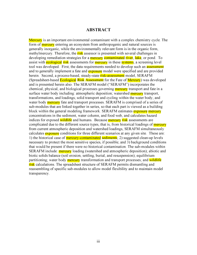
 ABSTRACT
Mercury is an important environmental contaminant with a complex chemistry cycle. The
form of mercury entering an ecosystem from anthropogenic and natural sources is
generally inorganic, while the environmentally relevant form is in the organic form,
methylmercury. Therefore, the risk assessor is presented with several challenges in
developing remediation strategies for a mercury contaminated river, lake, or pond. To
assist with ecological risk assessments for mercury in these systems, a screening level
tool was developed. First, the data requirements needed to develop such an assessment
and to generally implement a fate and exposure model were specified and are provided
herein. Second, a process-based, steady-state risk-assessment model, SERAFM
(Spreadsheet-based Ecological Risk Assessment for the Fate of Mercury) was developed
and is presented herein also. The SERAFM model ("SERAFM") incorporates the
chemical, physical, and biological processes governing mercury transport and fate in a
surface water body including: atmospheric deposition; watershed mercury transport,
transformations, and loadings; solid transport and cycling within the water body; and
water body mercury fate and transport processes. SERAFM is comprised of a series of
sub-modules that are linked together in series, so that each part is viewed as a building
block within the general modeling framework. SERAFM estimates exposure mercury
concentrations in the sediment, water column, and food web, and calculates hazard
indices for exposed wildlife and humans. Because mercury risk assessments are
complicated due to the different source types, that is, from historical loadings of mercury
from current atmospheric deposition and watershed loadings, SERAFM simultaneously
calculates exposure conditions for three different scenarios at any given site. These are:
1) the historical case of mercury-contaminated sediments; 2) suggested clean-up levels
necessary to protect the most sensitive species, if possible; and 3) background conditions
that would be present if there were no historical contamination. The sub-modules within
SERAFM include: mercury loading (watershed and atmospheric deposition); abiotic and
biotic solids balance (soil erosion, settling, burial, and resuspension); equilibrium
partitioning; water body mercury transformation and transport processes; and wildlife
risk calculations. The spreadsheet structure of SERAFM permits dismantling and
reassembling of specific sub-modules to allow model flexibility and to maintain model
transparency.
in
image:
ABSTRACT
Mercury is an important environmental contaminant with a complex chemistry cycle. The
form of mercury entering an ecosystem from anthropogenic and natural sources is
generally inorganic, while the environmentally relevant form is in the organic form,
methylmercury. Therefore, the risk assessor is presented with several challenges in
developing remediation strategies for a mercury contaminated river, lake, or pond. To
assist with ecological risk assessments for mercury in these systems, a screening level
tool was developed. First, the data requirements needed to develop such an assessment
and to generally implement a fate and exposure model were specified and are provided
herein. Second, a process-based, steady-state risk-assessment model, SERAFM
(Spreadsheet-based Ecological Risk Assessment for the Fate of Mercury) was developed
and is presented herein also. The SERAFM model ("SERAFM") incorporates the
chemical, physical, and biological processes governing mercury transport and fate in a
surface water body including: atmospheric deposition; watershed mercury transport,
transformations, and loadings; solid transport and cycling within the water body; and
water body mercury fate and transport processes. SERAFM is comprised of a series of
sub-modules that are linked together in series, so that each part is viewed as a building
block within the general modeling framework. SERAFM estimates exposure mercury
concentrations in the sediment, water column, and food web, and calculates hazard
indices for exposed wildlife and humans. Because mercury risk assessments are
complicated due to the different source types, that is, from historical loadings of mercury
from current atmospheric deposition and watershed loadings, SERAFM simultaneously
calculates exposure conditions for three different scenarios at any given site. These are:
1) the historical case of mercury-contaminated sediments; 2) suggested clean-up levels
necessary to protect the most sensitive species, if possible; and 3) background conditions
that would be present if there were no historical contamination. The sub-modules within
SERAFM include: mercury loading (watershed and atmospheric deposition); abiotic and
biotic solids balance (soil erosion, settling, burial, and resuspension); equilibrium
partitioning; water body mercury transformation and transport processes; and wildlife
risk calculations. The spreadsheet structure of SERAFM permits dismantling and
reassembling of specific sub-modules to allow model flexibility and to maintain model
transparency.
in
image:
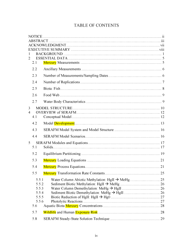
 TABLE OF CONTENTS
NOTICE ii
ABSTRACT iii
ACKNOWLEDGMENT vii
EXECUTIVE SUMMARY viii
1 BACKGROUND 1
2 ESSENTIAL DATA 5
2.1 Mercury Measurements 5
2.2 Ancillary Measurements 6
2.3 Number of Measurements/Sampling Dates 6
2.4 Number of Replications 7
2.5 Biota: Fish 8
2.6 Food Web 9
2.7 Water Body Characteristics 9
3 MODEL STRUCTURE 10
4 OVERVIEW of SERAFM 12
4.1 Conceptual Model 12
4.2 Model Development 13
4.3 SERAFM Model System and Model Structure 16
4.4 SERAFM Model Scenarios 16
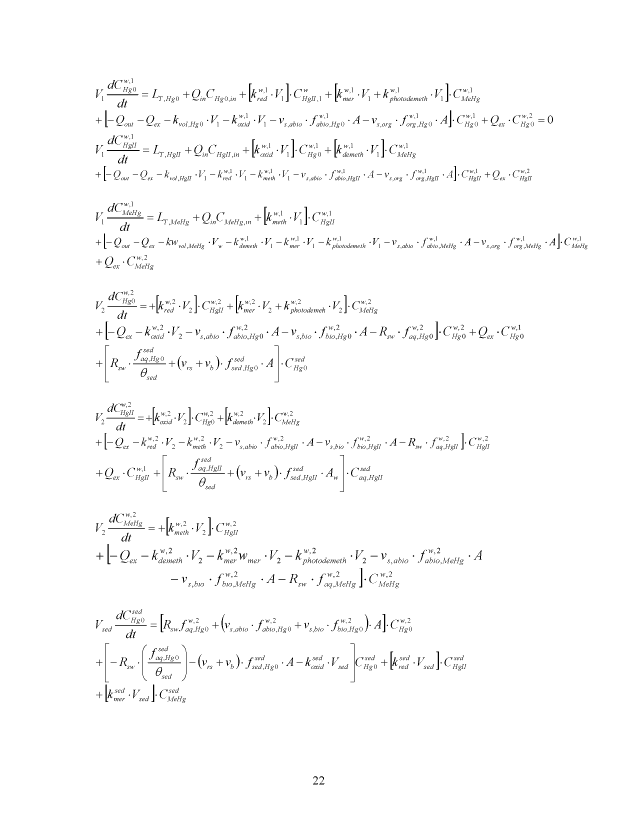
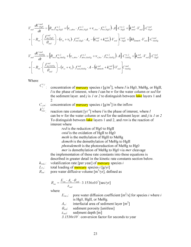
5 SERAFM Modules and Equations 17
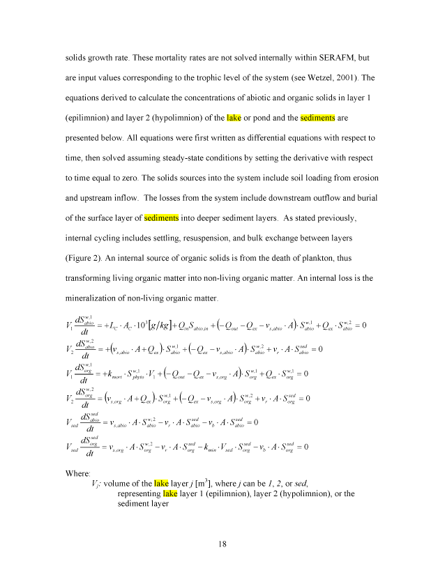
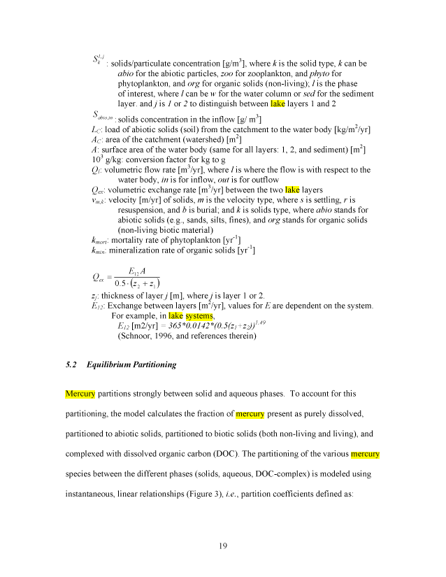
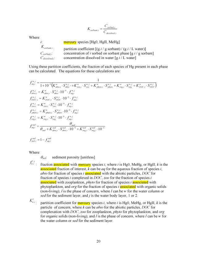
5.1 Solids 17
5.2 Equilibrium Partitioning 19
5.3 Mercury Loading Equations 21
5.4 Mercury Process Equations 21
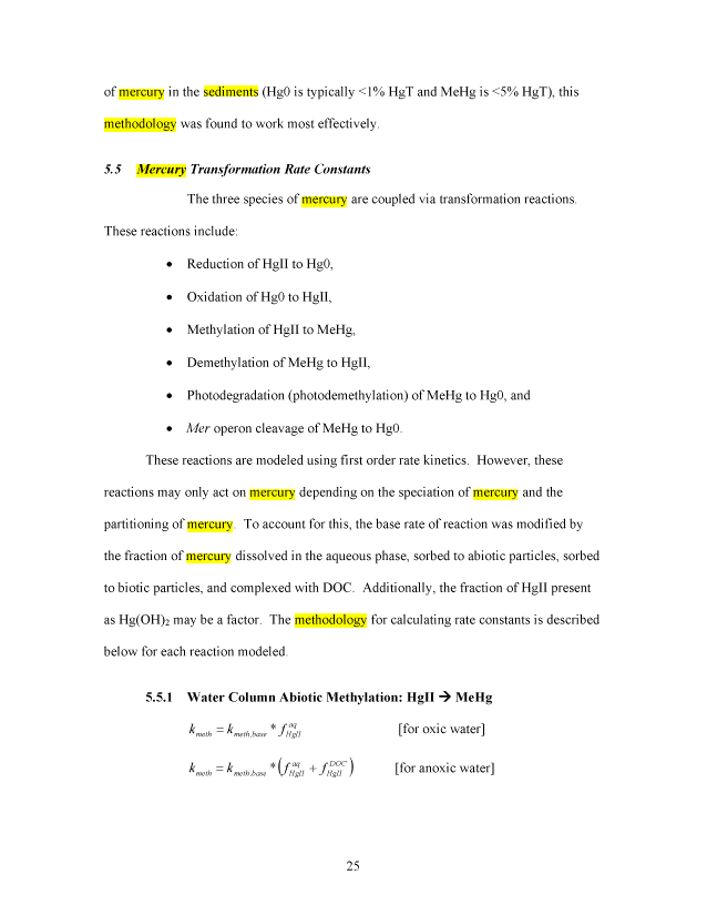
5.5 Mercury Transformation Rate Constants 25
5.5.1 Water Column Abiotic Methylation: Hgll -> MeHg 25
5.5.2 Sediment Biotic Methylation: Hgll -> MeHg 26
5.5.3 Water Column Demethylation: MeHg -> Hgll 26
5.5.4 Sediment Biotic Demethylation: MeHg -> Hgll 26
5.5.5 Biotic Reduction of Hgll: Hgll ^ HgO 27
5.5.6 Photolytic Reactions 27
5.6 Aquatic Biota Mercury Concentrations 28
5.7 Wildlife and Human Exposure Risk 28
5.8 SERAFM Steady-State Solution Technique 29
IV
image:
TABLE OF CONTENTS
NOTICE ii
ABSTRACT iii
ACKNOWLEDGMENT vii
EXECUTIVE SUMMARY viii
1 BACKGROUND 1
2 ESSENTIAL DATA 5
2.1 Mercury Measurements 5
2.2 Ancillary Measurements 6
2.3 Number of Measurements/Sampling Dates 6
2.4 Number of Replications 7
2.5 Biota: Fish 8
2.6 Food Web 9
2.7 Water Body Characteristics 9
3 MODEL STRUCTURE 10
4 OVERVIEW of SERAFM 12
4.1 Conceptual Model 12
4.2 Model Development 13
4.3 SERAFM Model System and Model Structure 16
4.4 SERAFM Model Scenarios 16
5 SERAFM Modules and Equations 17
5.1 Solids 17
5.2 Equilibrium Partitioning 19
5.3 Mercury Loading Equations 21
5.4 Mercury Process Equations 21
5.5 Mercury Transformation Rate Constants 25
5.5.1 Water Column Abiotic Methylation: Hgll -> MeHg 25
5.5.2 Sediment Biotic Methylation: Hgll -> MeHg 26
5.5.3 Water Column Demethylation: MeHg -> Hgll 26
5.5.4 Sediment Biotic Demethylation: MeHg -> Hgll 26
5.5.5 Biotic Reduction of Hgll: Hgll ^ HgO 27
5.5.6 Photolytic Reactions 27
5.6 Aquatic Biota Mercury Concentrations 28
5.7 Wildlife and Human Exposure Risk 28
5.8 SERAFM Steady-State Solution Technique 29
IV
image:
 6 MODEL INTERFACE LAYOUT 30
6.1 Input & Output Worksheet 31
6.1.1 Watershed Characteristics 31
6.1.2 Rate Constants 35
6.1.3 Exposure Concentrations 35
6.2 Human and Wildlife Exposure Risk Results 36
6.3 Wildlife Worksheet 36
6.4 Parameters Worksheet 36
6.5 Mercury Params Worksheet 37
6.6 Water Body Hg Worksheet 37
6.7 Water Body C sed Hg Worksheet 38
6.8 Target C sed Hg Worksheet 38
6.9 Hg Loading Worksheet 38
6.10 Gas Diff Loading Worksheet 39
6.11 Equilibrium Partitioning Worksheet 39
6.12 Solids Balance Worksheet 39
6.13 Rate Constants Worksheet 40
7 MODEL IMPLEMENTATION 40
7.1 Primary User Interface 40
7.2 Model Notes 41
8 REFERENCES 42
image:
6 MODEL INTERFACE LAYOUT 30
6.1 Input & Output Worksheet 31
6.1.1 Watershed Characteristics 31
6.1.2 Rate Constants 35
6.1.3 Exposure Concentrations 35
6.2 Human and Wildlife Exposure Risk Results 36
6.3 Wildlife Worksheet 36
6.4 Parameters Worksheet 36
6.5 Mercury Params Worksheet 37
6.6 Water Body Hg Worksheet 37
6.7 Water Body C sed Hg Worksheet 38
6.8 Target C sed Hg Worksheet 38
6.9 Hg Loading Worksheet 38
6.10 Gas Diff Loading Worksheet 39
6.11 Equilibrium Partitioning Worksheet 39
6.12 Solids Balance Worksheet 39
6.13 Rate Constants Worksheet 40
7 MODEL IMPLEMENTATION 40
7.1 Primary User Interface 40
7.2 Model Notes 41
8 REFERENCES 42
image:
 TABLES
Table 1. Proposed Tiers for Data Measurements for the ERASC Request No. 10:
Remediation Goals for Sediment Mercury
Table 2. Comparison of SERAFM and IEM-2M mercury concentrations using parameter
values for model ecosystem described in the Mercury Study Report to Congress
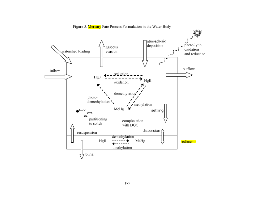
FIGURES
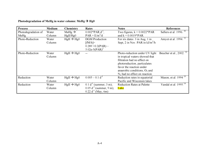
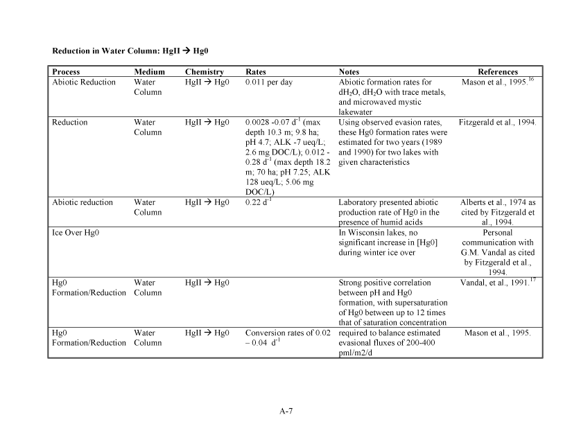
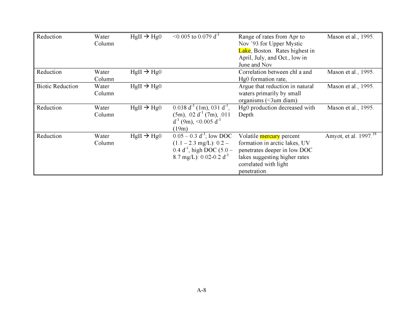
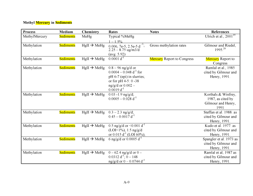
Figure 1. Mercury in the Environment
Figure 2. Solids Cycle in the Water Body
Figure 3. Equilibrium Partitioning of Mercury to Solids and DOC
Figure 4. Mercury Loading to the Water Body (Atmospheric and Watershed)
Figure 5. Mercury Processes in the Water Body'
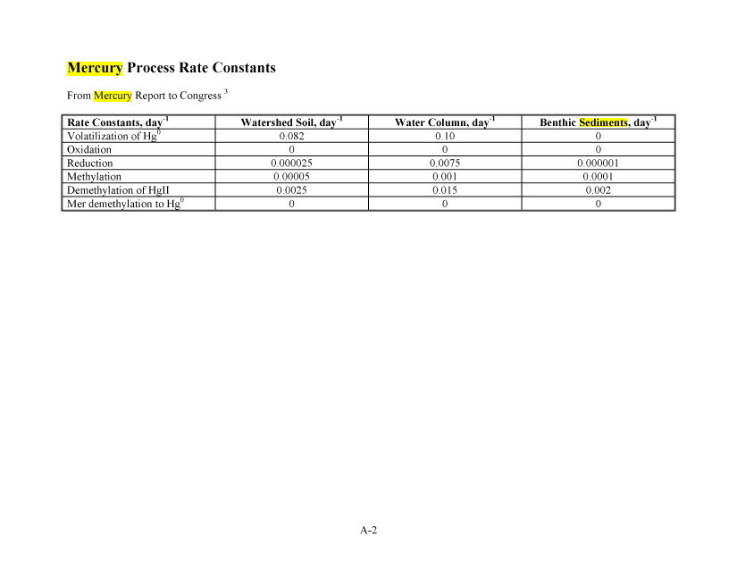
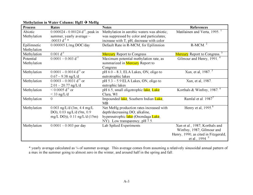
APPENDIX
Literature Mercury Process Rate Constants
VI
image:
TABLES
Table 1. Proposed Tiers for Data Measurements for the ERASC Request No. 10:
Remediation Goals for Sediment Mercury
Table 2. Comparison of SERAFM and IEM-2M mercury concentrations using parameter
values for model ecosystem described in the Mercury Study Report to Congress
FIGURES
Figure 1. Mercury in the Environment
Figure 2. Solids Cycle in the Water Body
Figure 3. Equilibrium Partitioning of Mercury to Solids and DOC
Figure 4. Mercury Loading to the Water Body (Atmospheric and Watershed)
Figure 5. Mercury Processes in the Water Body'
APPENDIX
Literature Mercury Process Rate Constants
VI
image:
 ACKNOWLEDGMENT
This work was performed in response to ERASC Request #10 (Ecological Risk
Assessment Support Center) under the direction of Michael Kravitz. The request was
made by Bart Hoskins, Region 1. Both provided suggestions in the development of both
the data requirements and the model itself. We would also like to thank Dale Hoff,
Region 8, for his review and comments.
vn
image:
ACKNOWLEDGMENT
This work was performed in response to ERASC Request #10 (Ecological Risk
Assessment Support Center) under the direction of Michael Kravitz. The request was
made by Bart Hoskins, Region 1. Both provided suggestions in the development of both
the data requirements and the model itself. We would also like to thank Dale Hoff,
Region 8, for his review and comments.
vn
image:
 EXECUTIVE SUMMARY
Mercury is of increasing environmental concern due to both its suspected toxicity and its
tendency to bioaccumulate and biomagnify in food webs. The United States
Environmental Protection Agency (US EPA) evaluated the mercury issue in 1997 in its
Mercury Study Report to Congress and targeted mercury as a primary area of research
interest. In 2003, the Ecosystems Research Division (ERD) of the National Exposure
Research Laboratory (NERL) in Athens, Georgia received Assistance Request Number
10 from the Ecological Risk Assessment Support Center (ERASC). This request was
designed specifically to target the question: How can we develop a remediation goal for
mercury in sediment when the concentration of mercury in sediment may be a poor
predictor of mercury exposure to biota? Additionally, this request also asked the related
questions: 1) What are the best ways to estimate mercury transfer (as methylmercury)
from sediment to the water column and/or the aquatic food chain, including birds and
mammals feeding upon fish and aquatic invertebrates? and 2) Should remediation goals
for mercury in sediment be developed for methylmercury only or, perhaps, total mercury
normalized for factors associated with methylation?
In an effort to address these questions, ERD developed a methodology that would assist a
regulator in deriving a remediation goal for sediments historically contaminated by
mercury in lake and river ecosystems. In this report, the process used to develop
remediation goals, including necessary data requirements, are described, and a tool is
provided to facilitate calculations of a remediation goal to protect fish and wildlife. This
Vlll
image:
EXECUTIVE SUMMARY
Mercury is of increasing environmental concern due to both its suspected toxicity and its
tendency to bioaccumulate and biomagnify in food webs. The United States
Environmental Protection Agency (US EPA) evaluated the mercury issue in 1997 in its
Mercury Study Report to Congress and targeted mercury as a primary area of research
interest. In 2003, the Ecosystems Research Division (ERD) of the National Exposure
Research Laboratory (NERL) in Athens, Georgia received Assistance Request Number
10 from the Ecological Risk Assessment Support Center (ERASC). This request was
designed specifically to target the question: How can we develop a remediation goal for
mercury in sediment when the concentration of mercury in sediment may be a poor
predictor of mercury exposure to biota? Additionally, this request also asked the related
questions: 1) What are the best ways to estimate mercury transfer (as methylmercury)
from sediment to the water column and/or the aquatic food chain, including birds and
mammals feeding upon fish and aquatic invertebrates? and 2) Should remediation goals
for mercury in sediment be developed for methylmercury only or, perhaps, total mercury
normalized for factors associated with methylation?
In an effort to address these questions, ERD developed a methodology that would assist a
regulator in deriving a remediation goal for sediments historically contaminated by
mercury in lake and river ecosystems. In this report, the process used to develop
remediation goals, including necessary data requirements, are described, and a tool is
provided to facilitate calculations of a remediation goal to protect fish and wildlife. This
Vlll
image:
 methodology is composed of two parts: Part One: essential data requirements; and Part
Two: screening-level mercury ecological risk assessment modeling framework. The
purpose of part one is to specifically provide a description of the essential data that a risk
project manager would need to obtain to establish a remediation goal for mercury in
sediments, as well as any other data that would be additionally useful. Part Two of this
project involves a description of the transport and fate processes required to derive the
remediation goal, and the creation of a modeling tool to aid in this endeavor.
In Part One, a progression of different types of data requirements is presented in three
tiers. The first tier presents the minimally essential data, the second tier presents useful
data that would increase the strength of the assessment, and the third tier presents the
most rigorous and most accurate approach for an assessment. The data requirements
specified herein include mercury measurements; ancillary measurements; number of
samples, including temporal, spatial and replication variability; fish tissue mercury
sampling; additional food web analysis measurements; and water body characteristics.
In Part Two, a spreadsheet modeling framework is presented that can be used as a risk
assessment tool for mercury contaminated surface water ecosystems. This model is the
SERAFM model ("SERAFM"), the Spreadsheet-based Ecological Risk Assessment for
the Fate of Mercury. In this tool, aprocess-based understanding of mercury is
incorporated into a steady-state modeling framework to assist with a wildlife risk
assessment.
IX
image:
methodology is composed of two parts: Part One: essential data requirements; and Part
Two: screening-level mercury ecological risk assessment modeling framework. The
purpose of part one is to specifically provide a description of the essential data that a risk
project manager would need to obtain to establish a remediation goal for mercury in
sediments, as well as any other data that would be additionally useful. Part Two of this
project involves a description of the transport and fate processes required to derive the
remediation goal, and the creation of a modeling tool to aid in this endeavor.
In Part One, a progression of different types of data requirements is presented in three
tiers. The first tier presents the minimally essential data, the second tier presents useful
data that would increase the strength of the assessment, and the third tier presents the
most rigorous and most accurate approach for an assessment. The data requirements
specified herein include mercury measurements; ancillary measurements; number of
samples, including temporal, spatial and replication variability; fish tissue mercury
sampling; additional food web analysis measurements; and water body characteristics.
In Part Two, a spreadsheet modeling framework is presented that can be used as a risk
assessment tool for mercury contaminated surface water ecosystems. This model is the
SERAFM model ("SERAFM"), the Spreadsheet-based Ecological Risk Assessment for
the Fate of Mercury. In this tool, aprocess-based understanding of mercury is
incorporated into a steady-state modeling framework to assist with a wildlife risk
assessment.
IX
image:
 A spreadsheet modeling environment was chosen for a few important reasons. A
spreadsheet provides a transparent and flexible working environment. The transparency
of the model is evident in that all the equations used for all calculations are easily viewed.
There are no hidden calculations. All manipulations that the model performs can be
easily reviewed and can readily be adapted or updated as needed. Similarly, a
spreadsheet can act as an inherent database to maintain all data and parameters.
Therefore, all parameters used and the values assigned to these parameters are presented
in a simple manner so that these can be changed or updated as needed. The modules
contained within the model itself are separated distinctly into individual worksheets.
Cross-referencing is performed across worksheets so that using the formula auditing tool
bar, all parameters can be simply traced back to their precedents and dependents. The
transparency of the model is enhanced by the flexibility it provides the user. The user
can change what is needed or let the default characteristics be used. This is a powerful
feature because the framework of this model can be used on a general, screening level
application or a more detailed and described system to investigate research questions.
The model was designed to simulate a watershed and associated water body that receives
atmospheric deposition of mercury and has had historical loadings of mercury to the
sediments, such as one associated with a facility of some kind that historically released
mercury to the watershed and/or water body. The SERAFM model runs its calculations
assuming steady-state and using process-based mathematical governing equations to
describe the fate and transport of mercury within the ecosystem. The SERAFM model
specifically calculates the mercury concentrations (Hgll, MeHg, HgO) in the water
image:
A spreadsheet modeling environment was chosen for a few important reasons. A
spreadsheet provides a transparent and flexible working environment. The transparency
of the model is evident in that all the equations used for all calculations are easily viewed.
There are no hidden calculations. All manipulations that the model performs can be
easily reviewed and can readily be adapted or updated as needed. Similarly, a
spreadsheet can act as an inherent database to maintain all data and parameters.
Therefore, all parameters used and the values assigned to these parameters are presented
in a simple manner so that these can be changed or updated as needed. The modules
contained within the model itself are separated distinctly into individual worksheets.
Cross-referencing is performed across worksheets so that using the formula auditing tool
bar, all parameters can be simply traced back to their precedents and dependents. The
transparency of the model is enhanced by the flexibility it provides the user. The user
can change what is needed or let the default characteristics be used. This is a powerful
feature because the framework of this model can be used on a general, screening level
application or a more detailed and described system to investigate research questions.
The model was designed to simulate a watershed and associated water body that receives
atmospheric deposition of mercury and has had historical loadings of mercury to the
sediments, such as one associated with a facility of some kind that historically released
mercury to the watershed and/or water body. The SERAFM model runs its calculations
assuming steady-state and using process-based mathematical governing equations to
describe the fate and transport of mercury within the ecosystem. The SERAFM model
specifically calculates the mercury concentrations (Hgll, MeHg, HgO) in the water
image:
 column (dissolved and total), in the food web (plankton, zooplankton, benthic
invertebrates, and trophic level 3 and 4 fish), and the hazard indices of exposed wildlife
and humans. The SERAFM model starts by calculating exposure concentrations for the
historical scenario, and from this case the most sensitive species (the species with the
highest hazard index) is identified. SERAFM then calculates exposure concentrations
and hazard indices for a scenario using only the effective background conditions, defined
as the conditions that the ecosystem would currently be under if it had never had
historical mercury loading. This scenario is particularly important to simulate because
ecosystems that are not receiving direct loadings of mercury still receive mercury loading
from the watershed and atmospheric deposition. Therefore, this scenario represents the
"best case" if all mercury from possible discharges or disposal practices had been
negated, and only current background conditions are influencing the system. Then, by
using the most sensitive species, the model does a simple linear approximation of what
the required sediment concentration would have to be to reduce the hazard index of the
most sensitive species to 1, and thus effectively protect all species associated with this
water body from mercury exposure. It is quite possible that because of the level of
mercury present in the current conditions that no level of remediation will recover the
system to sufficiently protect the most sensitive species. That is, current background
atmospheric and watershed loading of mercury to the water body is high enough to put
the most sensitive species at risk and until these inputs are reduced, the site will remain
above risk. All three scenarios are calculated instantaneously as parameters are changed.
XI
image:
column (dissolved and total), in the food web (plankton, zooplankton, benthic
invertebrates, and trophic level 3 and 4 fish), and the hazard indices of exposed wildlife
and humans. The SERAFM model starts by calculating exposure concentrations for the
historical scenario, and from this case the most sensitive species (the species with the
highest hazard index) is identified. SERAFM then calculates exposure concentrations
and hazard indices for a scenario using only the effective background conditions, defined
as the conditions that the ecosystem would currently be under if it had never had
historical mercury loading. This scenario is particularly important to simulate because
ecosystems that are not receiving direct loadings of mercury still receive mercury loading
from the watershed and atmospheric deposition. Therefore, this scenario represents the
"best case" if all mercury from possible discharges or disposal practices had been
negated, and only current background conditions are influencing the system. Then, by
using the most sensitive species, the model does a simple linear approximation of what
the required sediment concentration would have to be to reduce the hazard index of the
most sensitive species to 1, and thus effectively protect all species associated with this
water body from mercury exposure. It is quite possible that because of the level of
mercury present in the current conditions that no level of remediation will recover the
system to sufficiently protect the most sensitive species. That is, current background
atmospheric and watershed loading of mercury to the water body is high enough to put
the most sensitive species at risk and until these inputs are reduced, the site will remain
above risk. All three scenarios are calculated instantaneously as parameters are changed.
XI
image:
 This report is structured so that the user may take what he or she needs from it without
having to read it in its entirety. Each section presents a specific topic and can be used as
a reference. The background of the technical assistance request is presented in Section 1:
Introduction. The data requirements are presented in Section 2: Essential Data. The
structure and rationale of the model are presented in Section 3: Model Structure. In this
section, the reader will understand the compartmental structure of the model and how
each worksheet within the spreadsheet model interacts. A general overview of the
governing mercury transport and fate processes included in SERAFM and how the model
fits together is presented in Section 4: Overview of SERAFM. Section 5: SERAFM
Modules and Equations describes the general modules that fit together to comprise the
overall SERAFM modeling framework. In this section, the mathematical governing
equations are presented. The user primarily interacts with the "Input&Output" worksheet
that is described in Section 6: Model Interface Layout. This section also gives brief
details of the other worksheets. In Section 7: Model Implementation, details are
provided on how to use the model as a risk assessment tool. In this section, the user is
walked through a method of progressive calibration of the model. Since the model is
structured in module compartments, it is important to calibrate the model in a series of
steps on each level according to the module. Section 8: References lists all references
used in this work. The appendix provides a literature review of reported rate constants
for mercury transformation processes.
xn
image:
This report is structured so that the user may take what he or she needs from it without
having to read it in its entirety. Each section presents a specific topic and can be used as
a reference. The background of the technical assistance request is presented in Section 1:
Introduction. The data requirements are presented in Section 2: Essential Data. The
structure and rationale of the model are presented in Section 3: Model Structure. In this
section, the reader will understand the compartmental structure of the model and how
each worksheet within the spreadsheet model interacts. A general overview of the
governing mercury transport and fate processes included in SERAFM and how the model
fits together is presented in Section 4: Overview of SERAFM. Section 5: SERAFM
Modules and Equations describes the general modules that fit together to comprise the
overall SERAFM modeling framework. In this section, the mathematical governing
equations are presented. The user primarily interacts with the "Input&Output" worksheet
that is described in Section 6: Model Interface Layout. This section also gives brief
details of the other worksheets. In Section 7: Model Implementation, details are
provided on how to use the model as a risk assessment tool. In this section, the user is
walked through a method of progressive calibration of the model. Since the model is
structured in module compartments, it is important to calibrate the model in a series of
steps on each level according to the module. Section 8: References lists all references
used in this work. The appendix provides a literature review of reported rate constants
for mercury transformation processes.
xn
image:
 1 BACKGROUND
Mercury has been recognized as an important environmental pollutant by the United
States Environmental Protection Agency (USEPA) because of its suspected neurotoxicity
(USEPA, 1997). Mercury occurs naturally in the environment in its neutral, elemental
state (Hg°, HgO) as well as its oxidized, divalent state (Hg2+, Hgll). Mercury also exists
in the form of organometallics, such as the environmentally relevant compound
methylmercury (CH3Hg+, MeHg). The USEPA, the United States Food and Drug
Administration (FDA), and the European Food Safety Agency (EFSA) have recognized
that methylmercury is a contaminant of concern in announcing consumer advisories for
methylmercury concentrations in fish (USDHHS and USEPA, 2004; EFSA, 2004).
Methylmercury bioaccumulates (i.e.., increases in concentration in an organism
during its period of exposure) and biomagnifies (i.e., increases in concentration from
trophic level to trophic level (e.g.., from phytoplankton to zooplankton, to prey fish, to
predator fish) within a given food web. Methylmercury concentrations can increase
orders of magnitude from the aqueous methylmercury concentrations in lake water to
methylmercury tissue concentrations in higher trophic level organisms such as fish and
piscivorous birds and animals. The ingestion offish tissue contaminated with
methylmercury is the predominant exposure pathway for humans and wildlife. Wildlife
exposure to mercury can be of even greater concern than for humans because wildlife
survival sometimes relies on the exclusive consumption of aquatic organisms. The 2003
National Listing of Fish and Wildlife Advisories (NLFWA) by the USEPA reported that
there are 3,094 advisories for mercury in 48 states. These advisories represent 35% of
the nation's total lake acreage and 24% of the nation's total river miles. Approximately
1
image:
1 BACKGROUND
Mercury has been recognized as an important environmental pollutant by the United
States Environmental Protection Agency (USEPA) because of its suspected neurotoxicity
(USEPA, 1997). Mercury occurs naturally in the environment in its neutral, elemental
state (Hg°, HgO) as well as its oxidized, divalent state (Hg2+, Hgll). Mercury also exists
in the form of organometallics, such as the environmentally relevant compound
methylmercury (CH3Hg+, MeHg). The USEPA, the United States Food and Drug
Administration (FDA), and the European Food Safety Agency (EFSA) have recognized
that methylmercury is a contaminant of concern in announcing consumer advisories for
methylmercury concentrations in fish (USDHHS and USEPA, 2004; EFSA, 2004).
Methylmercury bioaccumulates (i.e.., increases in concentration in an organism
during its period of exposure) and biomagnifies (i.e., increases in concentration from
trophic level to trophic level (e.g.., from phytoplankton to zooplankton, to prey fish, to
predator fish) within a given food web. Methylmercury concentrations can increase
orders of magnitude from the aqueous methylmercury concentrations in lake water to
methylmercury tissue concentrations in higher trophic level organisms such as fish and
piscivorous birds and animals. The ingestion offish tissue contaminated with
methylmercury is the predominant exposure pathway for humans and wildlife. Wildlife
exposure to mercury can be of even greater concern than for humans because wildlife
survival sometimes relies on the exclusive consumption of aquatic organisms. The 2003
National Listing of Fish and Wildlife Advisories (NLFWA) by the USEPA reported that
there are 3,094 advisories for mercury in 48 states. These advisories represent 35% of
the nation's total lake acreage and 24% of the nation's total river miles. Approximately
1
image:
 101,818 lakes, 14,195,187 lake acres, and 846,310 river miles in the US are under
advisories. Additionally, 100% of the Great Lakes and their connecting waters are under
advisory (USEPA, 2004).
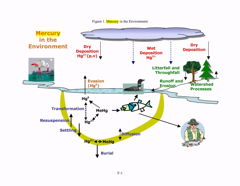
Mercury exhibits a complicated chemical cycle (see Figure 1). Mercury first
enters the global cycle through both anthropogenic and natural sources. Anthropogenic
point sources of mercury consist of combustion (e.g., utility boilers, municipal waste
combustors, commercial/industrial boilers, medical waste incinerators) and
manufacturing sources (e.g., chlor-alkali, cement, pulp and paper manufacturing)
(USEPA, 1997). Natural sources of mercury arise from geothermic emissions such as
crustal degassing in the deep ocean and volcanoes as well as dissolution of mercury from
geologic sources (Rasmussen, 1994). Because mercury has a residence time of
approximately one year in the atmosphere, emitted mercury can travel long distances
before depositing. Remote lakes that are otherwise not exposed to direct loadings of
mercury, such as those in eastern Canada, northeast and north central US, and
Scandinavia, have been reported to have high levels of mercury in both the water bodies
and fish (see Fitzgerald et al., 1998).
When mercury travels long distances through the atmosphere, it then deposits via
wet and dry deposition onto watersheds and water bodies. Deposited mercury can
undergo oxidation and reduction reactions that transform mercury from its divalent state
(Hgll) to its elemental state (HgO) and vice-versa. Additionally, bacteria can transform
mercury into the bioaccumulative and toxic form, MeHg. Once transformed, MeHg can
accumulate in aquatic vegetation and phytoplankton. Zooplankton then graze and
bioaccumulate the MeHg, which is subsequently transferred up the food chain to prey and
image:
101,818 lakes, 14,195,187 lake acres, and 846,310 river miles in the US are under
advisories. Additionally, 100% of the Great Lakes and their connecting waters are under
advisory (USEPA, 2004).
Mercury exhibits a complicated chemical cycle (see Figure 1). Mercury first
enters the global cycle through both anthropogenic and natural sources. Anthropogenic
point sources of mercury consist of combustion (e.g., utility boilers, municipal waste
combustors, commercial/industrial boilers, medical waste incinerators) and
manufacturing sources (e.g., chlor-alkali, cement, pulp and paper manufacturing)
(USEPA, 1997). Natural sources of mercury arise from geothermic emissions such as
crustal degassing in the deep ocean and volcanoes as well as dissolution of mercury from
geologic sources (Rasmussen, 1994). Because mercury has a residence time of
approximately one year in the atmosphere, emitted mercury can travel long distances
before depositing. Remote lakes that are otherwise not exposed to direct loadings of
mercury, such as those in eastern Canada, northeast and north central US, and
Scandinavia, have been reported to have high levels of mercury in both the water bodies
and fish (see Fitzgerald et al., 1998).
When mercury travels long distances through the atmosphere, it then deposits via
wet and dry deposition onto watersheds and water bodies. Deposited mercury can
undergo oxidation and reduction reactions that transform mercury from its divalent state
(Hgll) to its elemental state (HgO) and vice-versa. Additionally, bacteria can transform
mercury into the bioaccumulative and toxic form, MeHg. Once transformed, MeHg can
accumulate in aquatic vegetation and phytoplankton. Zooplankton then graze and
bioaccumulate the MeHg, which is subsequently transferred up the food chain to prey and
image:
 predator fish. These fish are then consumed by humans and wildlife, resulting in
accumulation of methylmercury in their tissue, which can result in toxic levels of
mercury. With each step up the food chain, mercury undergoes biomagnification,
resulting in higher and higher concentrations of mercury in each higher level organism.
Clearly, it is advantageous to understand the processes governing mercury cycling
so that we can adequately understand the level of risk to wildlife and humans exposed to
mercury from a given water body under various loading scenarios. There is a vast body
of literature describing the many different mercury transport and fate processes, and
recent research has furthered our understanding of the aggregate impact of watershed
loadings in addition to direct atmospheric loading. Patterns and correlations have been
investigated relating mercury concentrations in water to mercury concentrations in fish.
The USGS performed a national study investigating correlations between concentrations
of different species of mercury in a variety of media and the corresponding
concentrations of mercury in fish tissue. They found that bioaccumulation was strongly
correlated with MeHg concentration in water, but only moderately correlated with MeHg
concentration in sediment or total Hg concentration in water (Brumbaugh, 2001). These
observations provide a challenge to establish a basis adequately predicting fish mercury
concentrations. First, methylation of mercury is believed to occur predominately in the
sediments, and second, sites that have undergone direct inputs of mercury contamination
may have sediments contaminated well above background levels. The challenge then
arises as to how to handle exposure and risk assessments for aquatic ecosystems that have
had direct inputs of mercury to the water body and/or sediments. This is the crux of the
work presented in this report.
image:
predator fish. These fish are then consumed by humans and wildlife, resulting in
accumulation of methylmercury in their tissue, which can result in toxic levels of
mercury. With each step up the food chain, mercury undergoes biomagnification,
resulting in higher and higher concentrations of mercury in each higher level organism.
Clearly, it is advantageous to understand the processes governing mercury cycling
so that we can adequately understand the level of risk to wildlife and humans exposed to
mercury from a given water body under various loading scenarios. There is a vast body
of literature describing the many different mercury transport and fate processes, and
recent research has furthered our understanding of the aggregate impact of watershed
loadings in addition to direct atmospheric loading. Patterns and correlations have been
investigated relating mercury concentrations in water to mercury concentrations in fish.
The USGS performed a national study investigating correlations between concentrations
of different species of mercury in a variety of media and the corresponding
concentrations of mercury in fish tissue. They found that bioaccumulation was strongly
correlated with MeHg concentration in water, but only moderately correlated with MeHg
concentration in sediment or total Hg concentration in water (Brumbaugh, 2001). These
observations provide a challenge to establish a basis adequately predicting fish mercury
concentrations. First, methylation of mercury is believed to occur predominately in the
sediments, and second, sites that have undergone direct inputs of mercury contamination
may have sediments contaminated well above background levels. The challenge then
arises as to how to handle exposure and risk assessments for aquatic ecosystems that have
had direct inputs of mercury to the water body and/or sediments. This is the crux of the
work presented in this report.
image:
 Many sites often require that site remediation goals be developed for the
sediments instead of or in addition to those for the surface water. For these latter sites, it
is believed that the sediments are acting as a secondary source of mercury or as an
exposure medium for ecological receptors. For some contaminants, bioaccumulation
factors based on sediment contamination (e.g., BSAF: Biota-Sediment Accumulation
Factor) have been successfully developed and used as a direct correlation between the
sediment contaminant concentration and fish and/or wildlife contaminant concentrations.
The issue, therefore, remains to develop a protective remediation goal for mercury in
sediments, knowing that the concentration in the sediment may be a poor predictor of
mercury exposure to fish and wildlife. To this end, a steady-state, process-based mercury
cycling model has been created to assist a risk assessor or researcher to predict mercury
concentrations in the sediment, water column and fish in a given water body for a
specified watershed. The SERAFM, Spreadsheet-based Ecological Risk Assessment for
the Fate of Mercury, model predicts mercury concentrations for the species HgO, Hgll,
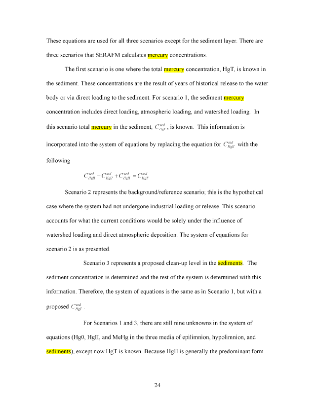
and MeHg. The model runs three simultaneous scenarios. One scenario is for
historically contaminated sediment, where the total mercury concentration in the
contaminated sediment is known. This scenario would be relevant, for example, for
modeling a Superfund site where the contaminated sediment is acting as a loading source
to the aquatic ecosystem. In this first scenario, the total mercury concentration in the
sediment is entered into the model as a known parameter. The second scenario is a
hypothetical background or reference condition, which is defined as the condition as if no
historical loading of mercury had occurred at this site. Therefore, the mercury
concentrations in both the water and sediment are calculated with no known mercury
image:
Many sites often require that site remediation goals be developed for the
sediments instead of or in addition to those for the surface water. For these latter sites, it
is believed that the sediments are acting as a secondary source of mercury or as an
exposure medium for ecological receptors. For some contaminants, bioaccumulation
factors based on sediment contamination (e.g., BSAF: Biota-Sediment Accumulation
Factor) have been successfully developed and used as a direct correlation between the
sediment contaminant concentration and fish and/or wildlife contaminant concentrations.
The issue, therefore, remains to develop a protective remediation goal for mercury in
sediments, knowing that the concentration in the sediment may be a poor predictor of
mercury exposure to fish and wildlife. To this end, a steady-state, process-based mercury
cycling model has been created to assist a risk assessor or researcher to predict mercury
concentrations in the sediment, water column and fish in a given water body for a
specified watershed. The SERAFM, Spreadsheet-based Ecological Risk Assessment for
the Fate of Mercury, model predicts mercury concentrations for the species HgO, Hgll,
and MeHg. The model runs three simultaneous scenarios. One scenario is for
historically contaminated sediment, where the total mercury concentration in the
contaminated sediment is known. This scenario would be relevant, for example, for
modeling a Superfund site where the contaminated sediment is acting as a loading source
to the aquatic ecosystem. In this first scenario, the total mercury concentration in the
sediment is entered into the model as a known parameter. The second scenario is a
hypothetical background or reference condition, which is defined as the condition as if no
historical loading of mercury had occurred at this site. Therefore, the mercury
concentrations in both the water and sediment are calculated with no known mercury
image:
 sediment concentration, but rather the total mercury concentration in the sediment is
directly calculated by the model. Mercury loadings to the water body are only from
direct atmospheric deposition to the water body and watershed, and subsequent erosion
and runoff. In this scenario, the water body sediment acts as a sink rather than a possible
source to the system. Using the calculated results of these two scenarios, a third scenario
is run to develop a proposed, possible sediment clean-up goal. This scenario uses a linear
extrapolation from the previous two scenarios to calculate the necessary sediment total
mercury concentration to protect the identified most sensitive species. Then, from this
information, the concentrations of mercury in the water body and fish tissue mercury
concentrations and the wildlife and human hazard indices are calculated as done in the
first scenario.
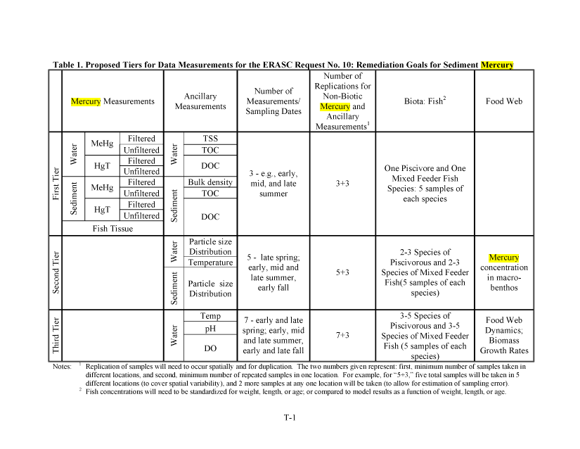
2 ESSENTIAL DATA
2.1 Mercury Measurements
There are three media of interest in these aquatic ecosystems: water column,
sediment, and fish tissue. The essential mercury data requirements in these media
consist of measuring the total mercury and methylmercury concentrations in both the
water and the sediment. For each of these measurements, both a filtered and unfiltered
sample are required. These data are required for all tiers, but the amount and extent of
samples vary tier by tier. Ancillary measurements are listed in Section 2.2. The details of
the necessary samples are presented in Sections 2.3 and 2.4. Mercury concentration in
fish tissue is also required, but this will be addressed further in Section 2.5. A summary
of the types of samples and number of suggested samples required is presented in Table
1.
image:
sediment concentration, but rather the total mercury concentration in the sediment is
directly calculated by the model. Mercury loadings to the water body are only from
direct atmospheric deposition to the water body and watershed, and subsequent erosion
and runoff. In this scenario, the water body sediment acts as a sink rather than a possible
source to the system. Using the calculated results of these two scenarios, a third scenario
is run to develop a proposed, possible sediment clean-up goal. This scenario uses a linear
extrapolation from the previous two scenarios to calculate the necessary sediment total
mercury concentration to protect the identified most sensitive species. Then, from this
information, the concentrations of mercury in the water body and fish tissue mercury
concentrations and the wildlife and human hazard indices are calculated as done in the
first scenario.
2 ESSENTIAL DATA
2.1 Mercury Measurements
There are three media of interest in these aquatic ecosystems: water column,
sediment, and fish tissue. The essential mercury data requirements in these media
consist of measuring the total mercury and methylmercury concentrations in both the
water and the sediment. For each of these measurements, both a filtered and unfiltered
sample are required. These data are required for all tiers, but the amount and extent of
samples vary tier by tier. Ancillary measurements are listed in Section 2.2. The details of
the necessary samples are presented in Sections 2.3 and 2.4. Mercury concentration in
fish tissue is also required, but this will be addressed further in Section 2.5. A summary
of the types of samples and number of suggested samples required is presented in Table
1.
image:
 2.2 Ancillary Measurements
There are several ancillary measurements that are also required for the water column
and the sediments. For tier one, the total organic carbon (TOC) and dissolved organic
carbon (DOC) concentrations must be measured in both the water and the sediment, as
well as the total suspended solids concentration in the water and the bulk density of the
sediments. For tier two, the particle size distributions in the water column and the
sediments are needed. Additionally, in tier two, the water temperature is measured. For
the third tier, water column dissolved oxygen (DO) and pH measurements are added.
2.3 Number of Measurements/Sampling Dates
The number of measurements taken affects the confidence in the measured value.
The statistical significance is increased with more samples. In the first tier, there are
three sampling dates: early, mid and late summer. The dates chosen coincide with the
greatest activity within a lake. During the summer months, the temperature in a lake
increases. This promotes faster fish growth and more bacterial activity (faster methylation
rates). Therefore, if only a few samples can be taken, it is important to at least get
samples during this most important summer time. If it is possible to take more samples,
then the breadth of sampling time frame can be increased to cover late spring and early
fall in tier two, and then early spring and late fall on into tier three. If the type of water
body that is being studied is believed to have appreciable parametric temporal variations,
then it may be important to increase the number of their measurements to capture this
variability. The number of measurements suggested here is the minimum number of
samples that would be required in our opinion.
image:
2.2 Ancillary Measurements
There are several ancillary measurements that are also required for the water column
and the sediments. For tier one, the total organic carbon (TOC) and dissolved organic
carbon (DOC) concentrations must be measured in both the water and the sediment, as
well as the total suspended solids concentration in the water and the bulk density of the
sediments. For tier two, the particle size distributions in the water column and the
sediments are needed. Additionally, in tier two, the water temperature is measured. For
the third tier, water column dissolved oxygen (DO) and pH measurements are added.
2.3 Number of Measurements/Sampling Dates
The number of measurements taken affects the confidence in the measured value.
The statistical significance is increased with more samples. In the first tier, there are
three sampling dates: early, mid and late summer. The dates chosen coincide with the
greatest activity within a lake. During the summer months, the temperature in a lake
increases. This promotes faster fish growth and more bacterial activity (faster methylation
rates). Therefore, if only a few samples can be taken, it is important to at least get
samples during this most important summer time. If it is possible to take more samples,
then the breadth of sampling time frame can be increased to cover late spring and early
fall in tier two, and then early spring and late fall on into tier three. If the type of water
body that is being studied is believed to have appreciable parametric temporal variations,
then it may be important to increase the number of their measurements to capture this
variability. The number of measurements suggested here is the minimum number of
samples that would be required in our opinion.
image:
 2.4 Number of Replications
In addition to capturing the temporal variation in the sampling, there needs to be
replication of the samples to increase the statistical significance of the measurements.
There are two types of errors associated with these types of measurements. First, there is
the spatial variability that occurs when sampling a heterogeneous media. Second, there is
the sampling error associated with any sample. To help understand the level of error
within each, it is prudent to independently account for both. To this end, we recommend
sampling in a manner that will allow estimation of these errors.
In Table 1, the column associated with the required/suggested data, the number of
replications suggested is presented as a number plus a number (i.e., m+n). The first
number, m, represents the number of different locations that should be sampled. The
second number, w, represents the number of replications suggested at any given location.
Therefore, for example, for a second tier study parameter measurement, this column
would show "5+3" samples. This designation yields a total of 7 unique samples; five
different locations are to be chosen and at four of these locations, only one sample would
be taken for each of the mercury and ancillary measurements, but at one location, a total
of three different samples would be taken, upon which the measurements will be made.
The five location samples are to assess spatial variability and the three co-located
samples provide information on the variability at any given sampling point. This scheme
helps one to determine if the range of each measured parameters is attributable to
sampling/measurement error or spatial variability. These various uncertainty factors can
then be incorporated in the model via Monte Carlo or other similar techniques
The "Replication" numbers presented in Table 1 for each of the three tiers are to be
perceived as suggested minimums. The more samples that can be taken will clearly
image:
2.4 Number of Replications
In addition to capturing the temporal variation in the sampling, there needs to be
replication of the samples to increase the statistical significance of the measurements.
There are two types of errors associated with these types of measurements. First, there is
the spatial variability that occurs when sampling a heterogeneous media. Second, there is
the sampling error associated with any sample. To help understand the level of error
within each, it is prudent to independently account for both. To this end, we recommend
sampling in a manner that will allow estimation of these errors.
In Table 1, the column associated with the required/suggested data, the number of
replications suggested is presented as a number plus a number (i.e., m+n). The first
number, m, represents the number of different locations that should be sampled. The
second number, w, represents the number of replications suggested at any given location.
Therefore, for example, for a second tier study parameter measurement, this column
would show "5+3" samples. This designation yields a total of 7 unique samples; five
different locations are to be chosen and at four of these locations, only one sample would
be taken for each of the mercury and ancillary measurements, but at one location, a total
of three different samples would be taken, upon which the measurements will be made.
The five location samples are to assess spatial variability and the three co-located
samples provide information on the variability at any given sampling point. This scheme
helps one to determine if the range of each measured parameters is attributable to
sampling/measurement error or spatial variability. These various uncertainty factors can
then be incorporated in the model via Monte Carlo or other similar techniques
The "Replication" numbers presented in Table 1 for each of the three tiers are to be
perceived as suggested minimums. The more samples that can be taken will clearly
image:
 provide more information and confidence in quantifying the variability at any given site
and in the model predictions. Ultimately, selection of the number of samples must
balance the scientific integrity of the project results with the economic feasibility and cost
of the project.
2.5 Biota: Fish
Fish tissue is the medium by which the transfer of mercury to wildlife occurs.
Therefore, to fully understand the overall transfer of mercury from the water and the
sediments, the fish tissue mercury concentration must be measured. As stated previously,
mercury bioaccumulates and species and biomagnifies with each transfer from lower
trophic level organisms to higher trophic level organisms. In this category of data
requirements, there are two types offish species (two trophic levels) for which the
mercury concentrations need to be determined, the piscivores and the mixed feeders. A
piscivore is a species offish that feeds primarily on other fish. A mixed feeder fish feeds
on fish but also on invertebrates.
For each species offish type sampled, five different measurements of mercury
concentration in the fish tissue must be made. Tier one, the simplest level, requires one
species of each type offish (i.e., piscivores and mixed feeder) be measured. For tier two,
2-3 species of each type is suggested; for tier three, 3 - 5 (or more) species of each type
is suggested (Table 1). Selecting more species of each type offish will give a more
rounded perspective of the food web and trophic transfer of mercury within the food web
itself.
An additional complication for measuring mercury in fish tissue is that there is a
direct correlation of the mercury concentration in fish with length, weight and age of the
image:
provide more information and confidence in quantifying the variability at any given site
and in the model predictions. Ultimately, selection of the number of samples must
balance the scientific integrity of the project results with the economic feasibility and cost
of the project.
2.5 Biota: Fish
Fish tissue is the medium by which the transfer of mercury to wildlife occurs.
Therefore, to fully understand the overall transfer of mercury from the water and the
sediments, the fish tissue mercury concentration must be measured. As stated previously,
mercury bioaccumulates and species and biomagnifies with each transfer from lower
trophic level organisms to higher trophic level organisms. In this category of data
requirements, there are two types offish species (two trophic levels) for which the
mercury concentrations need to be determined, the piscivores and the mixed feeders. A
piscivore is a species offish that feeds primarily on other fish. A mixed feeder fish feeds
on fish but also on invertebrates.
For each species offish type sampled, five different measurements of mercury
concentration in the fish tissue must be made. Tier one, the simplest level, requires one
species of each type offish (i.e., piscivores and mixed feeder) be measured. For tier two,
2-3 species of each type is suggested; for tier three, 3 - 5 (or more) species of each type
is suggested (Table 1). Selecting more species of each type offish will give a more
rounded perspective of the food web and trophic transfer of mercury within the food web
itself.
An additional complication for measuring mercury in fish tissue is that there is a
direct correlation of the mercury concentration in fish with length, weight and age of the
image:
 fish. Therefore, in addition to the fish tissue mercury concentration measurement, the
sampled fish's weights and lengths for each species from each type offish used must also
be measured. If possible, it would be quite useful if the age of the individual fishes
sampled could be determined as well. The modeler would then be able to account for the
variability of the measured mercury concentration due to fish weight, length, and/or age.
2.6 Food Web
The level of food web dynamics and the complications associated with it are an
important issue and concern in mercury modeling. Therefore, an increasingly more
rigorous system of modeling mercury transfer within the food web is used depending on
the assessment tier. In the first tier, correlations between the fish tissue mercury
concentration and the water and sediment concentrations are used. This is similar to a
more simplistic bioaccumulation factor approach. The bioaccumulation factor is to be
determined using site-specific data, and not simply literature data. In the second tier, a
trophic level mercury accumulation model is used. This model requires that the lower
trophic levels be modeled, and thus the mercury concentrations in the macro-benthos are
needed. For a third tier level assessment, a more rigorous food web model is used that
incorporates food web dynamics and the growth rates offish and other biota. This
approach will require calibration to the water body and ecosystem being investigated.
2.7 Water Body Characteristics
In addition to the herein specified mercury and ancillary measurements, it would be
most helpful if the parameters describing the water body were also provided. These
parameters mainly deal with the physical structure of the water body and its surrounding
environment. One important piece of information is the geometry of the water body, such
image:
fish. Therefore, in addition to the fish tissue mercury concentration measurement, the
sampled fish's weights and lengths for each species from each type offish used must also
be measured. If possible, it would be quite useful if the age of the individual fishes
sampled could be determined as well. The modeler would then be able to account for the
variability of the measured mercury concentration due to fish weight, length, and/or age.
2.6 Food Web
The level of food web dynamics and the complications associated with it are an
important issue and concern in mercury modeling. Therefore, an increasingly more
rigorous system of modeling mercury transfer within the food web is used depending on
the assessment tier. In the first tier, correlations between the fish tissue mercury
concentration and the water and sediment concentrations are used. This is similar to a
more simplistic bioaccumulation factor approach. The bioaccumulation factor is to be
determined using site-specific data, and not simply literature data. In the second tier, a
trophic level mercury accumulation model is used. This model requires that the lower
trophic levels be modeled, and thus the mercury concentrations in the macro-benthos are
needed. For a third tier level assessment, a more rigorous food web model is used that
incorporates food web dynamics and the growth rates offish and other biota. This
approach will require calibration to the water body and ecosystem being investigated.
2.7 Water Body Characteristics
In addition to the herein specified mercury and ancillary measurements, it would be
most helpful if the parameters describing the water body were also provided. These
parameters mainly deal with the physical structure of the water body and its surrounding
environment. One important piece of information is the geometry of the water body, such
image:
 as the width and length of a reach of river, or the surface area and depth of a lake or pond.
Additionally, the flow rate of a river and the lake/pond flushing rate (or hydraulic
residence time) will allow for mass balance calculations within the system. Watershed
loadings (as estimated from the size, land use, and wetland percentage) and upstream
mercury concentrations further assist in understanding the ecological impact of changes
in the studied/modeled water body sediment mercury concentration.
3 MODEL STRUCTURE
The model presented here is steady state and process based, incorporating a series
of modules such that each module fits into a scheme to simulate a comprehensive picture
of mercury exposure and risk. The model is written using Microsoft© Excel 2003
(Microsoft, Inc., 2003); it is implemented using a spreadsheet program for several
reasons. MS Excel is a program that is generally understood and used by the general
population, so it can be readily accessed and implemented by a wide audience. The user
does not need to understand higher level programming languages such as Visual Basic,
FORTRAN, or C++. Part of the expressed goal of this model development was to
incorporate the current state of the science in a readily available and easily implemented
software package to serve a greater variety of users. By being in a spreadsheet format, all
manipulations, parameters, and equations are readily available and transparent to the user.
This allows adjustments as the user sees fit. However, the model is organized with a
simple, upfront user interface so that higher level use can be performed without having to
dig into the depths of the program itself. Microsoft© Excel 2003 can act as its own
database, and the formula auditing toolbar allows tracking of precedent and dependent
cells. Additionally, a spreadsheet is a programming environment that allows each model
10
image:
as the width and length of a reach of river, or the surface area and depth of a lake or pond.
Additionally, the flow rate of a river and the lake/pond flushing rate (or hydraulic
residence time) will allow for mass balance calculations within the system. Watershed
loadings (as estimated from the size, land use, and wetland percentage) and upstream
mercury concentrations further assist in understanding the ecological impact of changes
in the studied/modeled water body sediment mercury concentration.
3 MODEL STRUCTURE
The model presented here is steady state and process based, incorporating a series
of modules such that each module fits into a scheme to simulate a comprehensive picture
of mercury exposure and risk. The model is written using Microsoft© Excel 2003
(Microsoft, Inc., 2003); it is implemented using a spreadsheet program for several
reasons. MS Excel is a program that is generally understood and used by the general
population, so it can be readily accessed and implemented by a wide audience. The user
does not need to understand higher level programming languages such as Visual Basic,
FORTRAN, or C++. Part of the expressed goal of this model development was to
incorporate the current state of the science in a readily available and easily implemented
software package to serve a greater variety of users. By being in a spreadsheet format, all
manipulations, parameters, and equations are readily available and transparent to the user.
This allows adjustments as the user sees fit. However, the model is organized with a
simple, upfront user interface so that higher level use can be performed without having to
dig into the depths of the program itself. Microsoft© Excel 2003 can act as its own
database, and the formula auditing toolbar allows tracking of precedent and dependent
cells. Additionally, a spreadsheet is a programming environment that allows each model
10
image:
 module to be separated into its own worksheet. This is effectively similar to having
distinct subroutines for each set of operations. The modules and their equations are
described in Section 5, and the details of each worksheet within the model spreadsheet
are detailed in Section 6: Model Interface Layout. Additionally, notes and equations are
provided in the spreadsheets themselves so that SERAFM can act as its own user's
manual.
The model itself consists of a series of modules; each solved independently using
a common parameter database and linked modules for input. Thereby, the model works
in a step-by-step fashion proceeding towards a solution for the desired parameters (e.g.,
fish mercury concentrations and wildlife hazard indices) in a feed-forward fashion. The
first module used in SERAFM calculates the total loading of each mercury species to the
water body. This module includes direct loading to the water body via wet and dry
deposition as well as indirect loading from watershed sources. Next, the solids balance
module calculates the concentrations of solids in the water body. Specifically, the
concentrations for abiotic, biotic, and organic solids are solved using a series of
simultaneous equations. The equations are derived as coupled differential equations that
are then solved assuming steady state conditions. Using the solutions for the solids
balances, the mercury cycling equations for the water body are solved. The mercury
equations are similarly derived as coupled differential equations that are solved
simultaneously assuming steady state conditions. Using the calculated mercury species
water column concentrations, bioaccumulation factors are used to predict mercury
concentrations in the different types of aquatic biota. Then, assuming daily ingestion
11
image:
module to be separated into its own worksheet. This is effectively similar to having
distinct subroutines for each set of operations. The modules and their equations are
described in Section 5, and the details of each worksheet within the model spreadsheet
are detailed in Section 6: Model Interface Layout. Additionally, notes and equations are
provided in the spreadsheets themselves so that SERAFM can act as its own user's
manual.
The model itself consists of a series of modules; each solved independently using
a common parameter database and linked modules for input. Thereby, the model works
in a step-by-step fashion proceeding towards a solution for the desired parameters (e.g.,
fish mercury concentrations and wildlife hazard indices) in a feed-forward fashion. The
first module used in SERAFM calculates the total loading of each mercury species to the
water body. This module includes direct loading to the water body via wet and dry
deposition as well as indirect loading from watershed sources. Next, the solids balance
module calculates the concentrations of solids in the water body. Specifically, the
concentrations for abiotic, biotic, and organic solids are solved using a series of
simultaneous equations. The equations are derived as coupled differential equations that
are then solved assuming steady state conditions. Using the solutions for the solids
balances, the mercury cycling equations for the water body are solved. The mercury
equations are similarly derived as coupled differential equations that are solved
simultaneously assuming steady state conditions. Using the calculated mercury species
water column concentrations, bioaccumulation factors are used to predict mercury
concentrations in the different types of aquatic biota. Then, assuming daily ingestion
11
image:
 rates of contaminated aquatic biota, hazard indices are estimated for the wildlife and
human receptors.
4 OVERVIEW of SERAFM
4.1 Conceptual Model
The following lists the overall conceptual model and module structure used to
simulate mercury fate and transport in this report:
• Atmospheric mercury deposition to the watershed and water body,
• Deposition processing by the watersheds followed by transport to the water
body via runoff, erosion, and tributaries,
• Mercury transformation processes in the water body:
o photolytic processes of oxidation, reduction, and degradation;
o biochemical and abiotic oxidation; and
o methylation and demethylation,
• Sorption and complexation processes to describe the partitioning of mercury
species to silts, sands, biotic solids, and dissolved and particulate organic matter,
• Settling to, resuspension from, and burial of particulates in sediments,
• Bioavailability of mercury complexes with hydroxides, chlorine, sulfide, and
dissolved organic carbon.
• Dissolved MeHg accumulation in aquatic vegetation, phytoplankton, and
benthic invertebrates, and zooplankton
• Bioaccumulation of MeHg through:
o fish predation of zooplankton and benthic invertebrates,
o fish preying on other fish.
12
image:
rates of contaminated aquatic biota, hazard indices are estimated for the wildlife and
human receptors.
4 OVERVIEW of SERAFM
4.1 Conceptual Model
The following lists the overall conceptual model and module structure used to
simulate mercury fate and transport in this report:
• Atmospheric mercury deposition to the watershed and water body,
• Deposition processing by the watersheds followed by transport to the water
body via runoff, erosion, and tributaries,
• Mercury transformation processes in the water body:
o photolytic processes of oxidation, reduction, and degradation;
o biochemical and abiotic oxidation; and
o methylation and demethylation,
• Sorption and complexation processes to describe the partitioning of mercury
species to silts, sands, biotic solids, and dissolved and particulate organic matter,
• Settling to, resuspension from, and burial of particulates in sediments,
• Bioavailability of mercury complexes with hydroxides, chlorine, sulfide, and
dissolved organic carbon.
• Dissolved MeHg accumulation in aquatic vegetation, phytoplankton, and
benthic invertebrates, and zooplankton
• Bioaccumulation of MeHg through:
o fish predation of zooplankton and benthic invertebrates,
o fish preying on other fish.
12
image:
 4.2 Model Development
SERAFM is the Spreadsheet-based Ecological Risk Assessment for the Fate of Mercury
model. The SERAFM model ("SERAFM") implements an updated set of the IEM-2M
solids and mercury fate algorithms described in detail in the Mercury Study Report to
Congress (USEPA, 1997). A comparison of SERAFM predicted results to those of IEM-
2M model using the parameter values for the model ecosystem described in the Report to
Congress is presented in Table 1. This preliminary comparison of the results of the two
models suggests that updates to the IEM-2M model incorporated into the SERAFM
model result in slightly lower predicted aqueous methylmercury concentrations and fish
tissue mercury concentrations, and slightly higher predicted aqueous total mercury
concentrations. The major differences between the SERAFM model and the IEM-2M
model are as follows:
• Watershed Loading: Both IEM-2M and SERAFM model soil erosion into the
water body using the Revised Universal Soil Loss Equation (RUSLE).
However, in SERAFM mercury loading from the watershed to the water
body is modeled using run-off coefficients. SERAFM defines and uses
four land-use types: impervious, upland, riparian, and wetland. The user
specifies the percentage of each land-use type in the watershed. The model
uses land-use specific run-off coefficients to transforms mercury loadings
to the watershed from atmospheric deposition to each land-use type into
loadings to the water body. SERAFM loadings to the watershed include
Hgll and MeHg loadings. In contrast, IEM-2M calculates the Hgll
concentrations in the watershed soils, accounts for reduction and
13
image:
4.2 Model Development
SERAFM is the Spreadsheet-based Ecological Risk Assessment for the Fate of Mercury
model. The SERAFM model ("SERAFM") implements an updated set of the IEM-2M
solids and mercury fate algorithms described in detail in the Mercury Study Report to
Congress (USEPA, 1997). A comparison of SERAFM predicted results to those of IEM-
2M model using the parameter values for the model ecosystem described in the Report to
Congress is presented in Table 1. This preliminary comparison of the results of the two
models suggests that updates to the IEM-2M model incorporated into the SERAFM
model result in slightly lower predicted aqueous methylmercury concentrations and fish
tissue mercury concentrations, and slightly higher predicted aqueous total mercury
concentrations. The major differences between the SERAFM model and the IEM-2M
model are as follows:
• Watershed Loading: Both IEM-2M and SERAFM model soil erosion into the
water body using the Revised Universal Soil Loss Equation (RUSLE).
However, in SERAFM mercury loading from the watershed to the water
body is modeled using run-off coefficients. SERAFM defines and uses
four land-use types: impervious, upland, riparian, and wetland. The user
specifies the percentage of each land-use type in the watershed. The model
uses land-use specific run-off coefficients to transforms mercury loadings
to the watershed from atmospheric deposition to each land-use type into
loadings to the water body. SERAFM loadings to the watershed include
Hgll and MeHg loadings. In contrast, IEM-2M calculates the Hgll
concentrations in the watershed soils, accounts for reduction and
13
image:
 instantaneous HgO evasion, then simulates transport of solids via erosion
and transport of Hgll via erosion and runoff to the water body.
Two-Layer: SERAFM has the capability to model a layered lake system with an
epilimnion and hypolimnion, while IEM-2M uses a single, well mixed
layer to represent the water column.
Photo-reactions: Recent research has demonstrated the importance of photolytic
transformations of mercury. These transformation processes have been
incorporated into SERAFM, but were not part of the original IEM-2M
model. In SERAFM, the photo-oxidation, photo-reduction, and photo-
degradation of mercury as functions of visible and UV-B light are
included, with specific light attenuation factors for each.
Speciation: Speciation of mercury with hydroxides, chlorides, and sulfides is
included in the SERAFM model but not in the IEM-2M model. Currently,
this difference only affects the effective oxidation rate constant of Hgll.
Future versions of SERAFM will expand its scope of modeling relative to
mercury speciation and its impact on mercury transformation rates as the
science of these processes is better understood.
Trophic status: Trophic status of the lake is taken into account in the SERAFM
model, but not the IEM-2M model. Trophic status is used to calculate
visible light attenuation in the lake, the turnover rate of biomass, and the
phytoplankton and zooplankton concentrations in the SERAFM model
framework.
14
image:
instantaneous HgO evasion, then simulates transport of solids via erosion
and transport of Hgll via erosion and runoff to the water body.
Two-Layer: SERAFM has the capability to model a layered lake system with an
epilimnion and hypolimnion, while IEM-2M uses a single, well mixed
layer to represent the water column.
Photo-reactions: Recent research has demonstrated the importance of photolytic
transformations of mercury. These transformation processes have been
incorporated into SERAFM, but were not part of the original IEM-2M
model. In SERAFM, the photo-oxidation, photo-reduction, and photo-
degradation of mercury as functions of visible and UV-B light are
included, with specific light attenuation factors for each.
Speciation: Speciation of mercury with hydroxides, chlorides, and sulfides is
included in the SERAFM model but not in the IEM-2M model. Currently,
this difference only affects the effective oxidation rate constant of Hgll.
Future versions of SERAFM will expand its scope of modeling relative to
mercury speciation and its impact on mercury transformation rates as the
science of these processes is better understood.
Trophic status: Trophic status of the lake is taken into account in the SERAFM
model, but not the IEM-2M model. Trophic status is used to calculate
visible light attenuation in the lake, the turnover rate of biomass, and the
phytoplankton and zooplankton concentrations in the SERAFM model
framework.
14
image:
 • Suspended particle types in the water column: The SERAFM model accounts
for both zooplankton and phytoplankton as biotic materials in the system;
the IEM-2M model accounts for one general biotic particle type.
• Reaction rates: The SERAFM model incorporates more recent transformation
reaction rate coefficients and understanding of the variability of these rates
under different conditions.
• Partition coefficients: The SERAFM model incorporates more recent values for
mercury partition coefficients for each mercury species. Future versions of
SERAFM will calculate site-specific partitioning as a function of sediment
organic matter and the organic carbon content of suspended materials.
State variables in both the IEM-2M and SERAFM models include three mercury
species, HgO, Hgll, and MeHg. As mentioned previously, SERAFM includes four solids
types (abiotic solids, phytoplankton solids, zooplankton solids, and detrital solids) plus
dissolved organic carbon, DOC. Both IEM-2M and SERAFM simulations are driven by
external mercury loadings delivered from the atmosphere, from watershed tributaries, and
from point sources, or by internal loadings from contaminated sediments. SERAFM
calculates the time-dependent mercury species concentrations in the water column and
sediments of the specified water body. Hgll and MeHg are partitioned to suspended and
benthic solids and complexed with DOC with user-specified or SERAFM default
partition coefficients for each sorbent type. Also, In SERAFM, mercury species are
subject to several transformation reactions, including photo-oxidation and dark oxidation
of HgO in the water column, photo-reduction and methylation of Hgll in the water
column and sediment layers, and photo-degradation and demethylation of MeHg in the
15
image:
• Suspended particle types in the water column: The SERAFM model accounts
for both zooplankton and phytoplankton as biotic materials in the system;
the IEM-2M model accounts for one general biotic particle type.
• Reaction rates: The SERAFM model incorporates more recent transformation
reaction rate coefficients and understanding of the variability of these rates
under different conditions.
• Partition coefficients: The SERAFM model incorporates more recent values for
mercury partition coefficients for each mercury species. Future versions of
SERAFM will calculate site-specific partitioning as a function of sediment
organic matter and the organic carbon content of suspended materials.
State variables in both the IEM-2M and SERAFM models include three mercury
species, HgO, Hgll, and MeHg. As mentioned previously, SERAFM includes four solids
types (abiotic solids, phytoplankton solids, zooplankton solids, and detrital solids) plus
dissolved organic carbon, DOC. Both IEM-2M and SERAFM simulations are driven by
external mercury loadings delivered from the atmosphere, from watershed tributaries, and
from point sources, or by internal loadings from contaminated sediments. SERAFM
calculates the time-dependent mercury species concentrations in the water column and
sediments of the specified water body. Hgll and MeHg are partitioned to suspended and
benthic solids and complexed with DOC with user-specified or SERAFM default
partition coefficients for each sorbent type. Also, In SERAFM, mercury species are
subject to several transformation reactions, including photo-oxidation and dark oxidation
of HgO in the water column, photo-reduction and methylation of Hgll in the water
column and sediment layers, and photo-degradation and demethylation of MeHg in the
15
image:
 water column and sediment layers. Water column oxidation, reduction and demethylation
reactions are driven by sunlight, and so their input rate constants are attenuated through
the water column using specified light extinction coefficients. HgO is subject to volatile
exchange between the water column and the atmosphere governed by a transfer rate
calculated from wind velocity and water depth, and by its Henry's Law constant.
4.3 SERAFM Model System and Model Structure
SERAFM is a steady state, process based model incorporating a series of modules, with
each module fitting into the scheme of mercury modeling to create a complete picture of
mercury exposure and risk. SERAFM is structured using Microsoft© Excel 2003
(Microsoft, Inc., 2003) to keep each sub-module separated from other sub-modules. Each
sub-module is housed on a separate worksheet within the Microsoft Excel workbook that
all together comprises SERAFM. This, in effect, is of similar design to having each sub-
module within its own subroutine in a more formal programming language. The primary
worksheet is the "Input & Output" worksheet that houses the model input and the model
base rate constants for mercury transformations in the water body and sediments.
SERAFM uses these input values and base rate constants, and calls on the remaining
worksheets within the workbook to instantaneously calculate the output results. These
output results are presented as the modeled exposure concentrations on the same
worksheet as the input parameters.
4.4 SERAFM Model Scenarios
SERAFM is structured to investigate and solve three scenarios to assist with the
development of a remediation strategy for aquatic ecosystems with mercury-
16
image:
water column and sediment layers. Water column oxidation, reduction and demethylation
reactions are driven by sunlight, and so their input rate constants are attenuated through
the water column using specified light extinction coefficients. HgO is subject to volatile
exchange between the water column and the atmosphere governed by a transfer rate
calculated from wind velocity and water depth, and by its Henry's Law constant.
4.3 SERAFM Model System and Model Structure
SERAFM is a steady state, process based model incorporating a series of modules, with
each module fitting into the scheme of mercury modeling to create a complete picture of
mercury exposure and risk. SERAFM is structured using Microsoft© Excel 2003
(Microsoft, Inc., 2003) to keep each sub-module separated from other sub-modules. Each
sub-module is housed on a separate worksheet within the Microsoft Excel workbook that
all together comprises SERAFM. This, in effect, is of similar design to having each sub-
module within its own subroutine in a more formal programming language. The primary
worksheet is the "Input & Output" worksheet that houses the model input and the model
base rate constants for mercury transformations in the water body and sediments.
SERAFM uses these input values and base rate constants, and calls on the remaining
worksheets within the workbook to instantaneously calculate the output results. These
output results are presented as the modeled exposure concentrations on the same
worksheet as the input parameters.
4.4 SERAFM Model Scenarios
SERAFM is structured to investigate and solve three scenarios to assist with the
development of a remediation strategy for aquatic ecosystems with mercury-
16
image:
 contaminated sediments. Scenario 1 is for the current conditions of a site that has been
subject to historical loading of mercury. An example of this type of site is one associated
with an industrial facility that released mercury into a nearby water body. Over time, the
mercury settled into the sediments, which resulted in increased mercury concentrations in
the sediment over background or reference conditions. This sediment concentration can
therefore act as an additional source over time to the associated water body. Scenario 2 is
the same site as if there had never been an industrial site. This is an effective background
or reference condition. In this scenario, the water body and sediments have undergone
mercury loading solely through atmospheric and watershed loading. There is still
mercury in the system, but it is not the result of industrial loading over time. Scenario 3
is a hypothetical scenario where Scenario 1 has undergone remediation to reduce the
mercury concentrations in the sediment. By using the information in Scenario 1 and 2,
Scenario 3 estimates the mercury concentration in the sediment that would be necessary
to protect the most sensitive ecological receptor.
5 SERAFM Modules and Equations
5.1 Solids
The steady-state concentrations of abiotic and organic solids in the water body are
simulated in the solids balance module that is separate from the module containing the
mercury process equations. A set of simultaneous equations were derived to calculate the
concentration of the abiotic solids, abio and organic solids, org. The abiotic solids
account for soil particles (sands, silts, and fines), and the organic solids account for the
non-living organic solids. Because SERAFM is a steady-state model, the living biota
(zooplankton and phytoplankton) turnover rate (mortality rate) is equal to the organic
17
image:
contaminated sediments. Scenario 1 is for the current conditions of a site that has been
subject to historical loading of mercury. An example of this type of site is one associated
with an industrial facility that released mercury into a nearby water body. Over time, the
mercury settled into the sediments, which resulted in increased mercury concentrations in
the sediment over background or reference conditions. This sediment concentration can
therefore act as an additional source over time to the associated water body. Scenario 2 is
the same site as if there had never been an industrial site. This is an effective background
or reference condition. In this scenario, the water body and sediments have undergone
mercury loading solely through atmospheric and watershed loading. There is still
mercury in the system, but it is not the result of industrial loading over time. Scenario 3
is a hypothetical scenario where Scenario 1 has undergone remediation to reduce the
mercury concentrations in the sediment. By using the information in Scenario 1 and 2,
Scenario 3 estimates the mercury concentration in the sediment that would be necessary
to protect the most sensitive ecological receptor.
5 SERAFM Modules and Equations
5.1 Solids
The steady-state concentrations of abiotic and organic solids in the water body are
simulated in the solids balance module that is separate from the module containing the
mercury process equations. A set of simultaneous equations were derived to calculate the
concentration of the abiotic solids, abio and organic solids, org. The abiotic solids
account for soil particles (sands, silts, and fines), and the organic solids account for the
non-living organic solids. Because SERAFM is a steady-state model, the living biota
(zooplankton and phytoplankton) turnover rate (mortality rate) is equal to the organic
17
image:
 solids growth rate. These mortality rates are not solved internally within SERAFM, but
are input values corresponding to the trophic level of the system (see Wetzel, 2001). The
equations derived to calculate the concentrations of abiotic and organic solids in layer 1
(epilimnion) and layer 2 (hypolimnion) of the lake or pond and the sediments are
presented below. All equations were first written as differential equations with respect to
time, then solved assuming steady-state conditions by setting the derivative with respect
to time equal to zero. The solids sources into the system include soil loading from erosion
and upstream inflow. The losses from the system include downstream outflow and burial
of the surface layer of sediments into deeper sediment layers. As stated previously,
internal cycling includes settling, resuspension, and bulk exchange between layers
(Figure 2). An internal source of organic solids is from the death of plankton, thus
transforming living organic matter into non-living organic matter. An internal loss is the
mineralization of non-living organic matter.
/, L. c L<J i <J j ^in abiojn \ Z--out z--ex s.abio
at
i^Mo_ = +(v -A + O \SW:1 + (-O -v .. -A]-SW:2 +v -A-S^ =0
7 V s,abio z-<ex! abio \ z-<ex s,abio / abio r abio
dSorg w,l ( \ w,l ,,1 _
^^^~^^^~ — "T~/C ,"O j f * r i "T" \ \J f \J v ' ./T /" O "T" V-/ " O — V/
/, vnoYi pnyio l \ •s-'Owr -s-^fix 5 orj? / orj? -s-^sx ory
at
org
'. 7, ~ \vs,org ' •rL~r'xiex)'^org ' \ t^ex ' s.org '•'-) "org ' 'r " ^org
- (v .A+n \^w'l+(-D -v • A\- Vw'2 +v • A- ^sed - 0
~Vs.org A+(^-ex) ^ org + \ \Lex Vs,org A! ^ org + Vr A ^ org ~U
y "•^abio _ A. C"1-2 _ v A. ?sed -v . A . <?sed - 0
y sed ,, - Vs,abio A ^abio Vr A ° abio Vb A ^ Mo ~ U
at
dSsed
y ors - v A. e*-2 _ v . A . <?sed -if .77 . <?sed - v • A • Vsed - 0
* sed , ~ Vs,org ^ ° ' org Vr ^ ° ' org ^min y sed ° org Vb ^ ° org ~V
Where:
Vf. volume of the lake layery [m3], wherey can be 7, 2, or sed,
representing lake layer 1 (epilimnion), layer 2 (hypolimnion), or the
sediment layer
18
image:
solids growth rate. These mortality rates are not solved internally within SERAFM, but
are input values corresponding to the trophic level of the system (see Wetzel, 2001). The
equations derived to calculate the concentrations of abiotic and organic solids in layer 1
(epilimnion) and layer 2 (hypolimnion) of the lake or pond and the sediments are
presented below. All equations were first written as differential equations with respect to
time, then solved assuming steady-state conditions by setting the derivative with respect
to time equal to zero. The solids sources into the system include soil loading from erosion
and upstream inflow. The losses from the system include downstream outflow and burial
of the surface layer of sediments into deeper sediment layers. As stated previously,
internal cycling includes settling, resuspension, and bulk exchange between layers
(Figure 2). An internal source of organic solids is from the death of plankton, thus
transforming living organic matter into non-living organic matter. An internal loss is the
mineralization of non-living organic matter.
/, L. c L<J i <J j ^in abiojn \ Z--out z--ex s.abio
at
i^Mo_ = +(v -A + O \SW:1 + (-O -v .. -A]-SW:2 +v -A-S^ =0
7 V s,abio z-<ex! abio \ z-<ex s,abio / abio r abio
dSorg w,l ( \ w,l ,,1 _
^^^~^^^~ — "T~/C ,"O j f * r i "T" \ \J f \J v ' ./T /" O "T" V-/ " O — V/
/, vnoYi pnyio l \ •s-'Owr -s-^fix 5 orj? / orj? -s-^sx ory
at
org
'. 7, ~ \vs,org ' •rL~r'xiex)'^org ' \ t^ex ' s.org '•'-) "org ' 'r " ^org
- (v .A+n \^w'l+(-D -v • A\- Vw'2 +v • A- ^sed - 0
~Vs.org A+(^-ex) ^ org + \ \Lex Vs,org A! ^ org + Vr A ^ org ~U
y "•^abio _ A. C"1-2 _ v A. ?sed -v . A . <?sed - 0
y sed ,, - Vs,abio A ^abio Vr A ° abio Vb A ^ Mo ~ U
at
dSsed
y ors - v A. e*-2 _ v . A . <?sed -if .77 . <?sed - v • A • Vsed - 0
* sed , ~ Vs,org ^ ° ' org Vr ^ ° ' org ^min y sed ° org Vb ^ ° org ~V
Where:
Vf. volume of the lake layery [m3], wherey can be 7, 2, or sed,
representing lake layer 1 (epilimnion), layer 2 (hypolimnion), or the
sediment layer
18
image:
 Slj 3
k : solids/particulate concentration [g/m ], where k is the solid type, k can be
abio for the abiotic particles, zoo for zooplankton, andphyto for
phytoplankton, and org for organic solids (non-living); / is the phase
of interest, where / can be w for the water column or sed for the sediment
layer, andy is 7 or 2 to distinguish between lake layers 1 and 2
o
^ *>ZM'^ l',* 1*1 J J * * J 1 * fl l~/3~l
concentration in the inflow [g/ m ]
LC'. load of abiotic solids (soil) from the catchment to the water body [kg/m2/yr]
AC', area of the catchment (watershed) [m2]
A: surface area of the water body (same for all layers: 1, 2, and sediment) [m2]
103 g/kg: conversion factor for kg to g
Qi. volumetric flow rate [m3/yr], where / is where the flow is with respect to the
water body, in is for inflow, out is for outflow
Qex: volumetric exchange rate [m3/yr] between the two lake layers
Vmfr. velocity [m/yr] of solids, m is the velocity type, where s is settling, r is
resuspension, and b is burial; and k is solids type, where abio stands for
abiotic solids (e.g., sands, silts, fines), and org stands for organic solids
(non-living biotic material)
kmort: mortality rate of phytoplankton [yr"1]
kmin. mineralization rate of organic solids [yr"1]
zf. thickness of layery [m], where y is layer 1 or 2.
£12: Exchange between layers [m2/yr], values for E are dependent on the system.
For example, in lake systems,
Ei 2 [m2/yr] = 365*0.0142*
(Schnoor, 1996, and references therein)
i 2 [m2/yr] = 365*0.0142*(0.5(Zl+z2))L49
5.2 Equilibrium Partitioning
Mercury partitions strongly between solid and aqueous phases. To account for this
partitioning, the model calculates the fraction of mercury present as purely dissolved,
partitioned to abiotic solids, partitioned to biotic solids (both non-living and living), and
complexed with dissolved organic carbon (DOC). The partitioning of the various mercury
species between the different phases (solids, aqueous, DOC-complex) is modeled using
instantaneous, linear relationships (Figure 3), i.e., partition coefficients defined as:
19
image:
Slj 3
k : solids/particulate concentration [g/m ], where k is the solid type, k can be
abio for the abiotic particles, zoo for zooplankton, andphyto for
phytoplankton, and org for organic solids (non-living); / is the phase
of interest, where / can be w for the water column or sed for the sediment
layer, andy is 7 or 2 to distinguish between lake layers 1 and 2
o
^ *>ZM'^ l',* 1*1 J J * * J 1 * fl l~/3~l
concentration in the inflow [g/ m ]
LC'. load of abiotic solids (soil) from the catchment to the water body [kg/m2/yr]
AC', area of the catchment (watershed) [m2]
A: surface area of the water body (same for all layers: 1, 2, and sediment) [m2]
103 g/kg: conversion factor for kg to g
Qi. volumetric flow rate [m3/yr], where / is where the flow is with respect to the
water body, in is for inflow, out is for outflow
Qex: volumetric exchange rate [m3/yr] between the two lake layers
Vmfr. velocity [m/yr] of solids, m is the velocity type, where s is settling, r is
resuspension, and b is burial; and k is solids type, where abio stands for
abiotic solids (e.g., sands, silts, fines), and org stands for organic solids
(non-living biotic material)
kmort: mortality rate of phytoplankton [yr"1]
kmin. mineralization rate of organic solids [yr"1]
zf. thickness of layery [m], where y is layer 1 or 2.
£12: Exchange between layers [m2/yr], values for E are dependent on the system.
For example, in lake systems,
Ei 2 [m2/yr] = 365*0.0142*
(Schnoor, 1996, and references therein)
i 2 [m2/yr] = 365*0.0142*(0.5(Zl+z2))L49
5.2 Equilibrium Partitioning
Mercury partitions strongly between solid and aqueous phases. To account for this
partitioning, the model calculates the fraction of mercury present as purely dissolved,
partitioned to abiotic solids, partitioned to biotic solids (both non-living and living), and
complexed with dissolved organic carbon (DOC). The partitioning of the various mercury
species between the different phases (solids, aqueous, DOC-complex) is modeled using
instantaneous, linear relationships (Figure 3), i.e., partition coefficients defined as:
19
image:
 f
JT^ sorbed,i
sorbant,i ^
dissolved,i
Where:
/': mercury species [HgO, Hgll, MeHg]
V
sorbant,:. partition coefficient [(g /' / g sorbant) / (g / / L water)]
Csorbed/- concentration of /' sorbed on sorbant phase [g / / g sorbant]
Cdissolved/- concentration dissolved in water [g / / L water]
Using these partition coefficients, the fraction of each species of Hg present in each phase
can be calculated. The equations for these calculations are:
J aq,i
_ _ _ _
1 i 1 (\-6(Yw CWJ' ±YW C"*1,;' i V™ C*,;' i V-™ owj , TfVi ctwj \
1 -I- 1U \J^abio,i ' '-'abio ' ~^*^zoo,i ' ^ zoo ~"~ ^ phyto, i ' ° phyto ^^org.i ' ° org ~"~ ^ DOC ,i ' ° DOC )
aq,i
fw,j — V~w _ owj _ i rv-6 _ fw.j
JDOC,i ~ DOC,i ' °DOC ' J aq,i
rW,j =K* .S».J .IQ-6. f».J
J zoo,i zoo,i zoo J aq,i
J phytoj p~hyto,i phyto J aq,i
™,j =K* .$*>] .IQ-6 . f*J
J org,i org,i org J aq,i
9
fsed _ L> sed
d cised i rv-6 . j^sed cised i rv-6
ab,o,, • ^ ab,o,, ~W +KOrg,,^ org,, ' [ °
rsed _ i rsed
J sed,i J aq,i
Where:
Osed'. sediment porosity [unitless]
fi.j
Jk-1 : fraction associated with mercury species /', where /' is HgO, MeHg, or Hgll; k is the
associated fraction of interest, k can be aq for the aqueous fraction of species /',
abio for fraction of species /' associated with the abiotic particles, DOC for
fraction of species /' complexed in DOC, zoo for the fraction of species /'
associated with zooplankton, phyto for fraction of species /' associated with
phytoplankton, and org for the fraction of species /' associated with organic solids
(non-living); / is the phase of concern, where / can be w for the water column or
sedfor the sediment layer; andy' is the water body layer, 1 or 2.
K1
kj : partition coefficient for mercury species /', where /' is HgO, MeHg, or Hgll; k is the
particle of concern, where k can be abio for the abiotic particles, DOC for
complexation with DOC, zoo for zooplankton, phyto for phytoplankton, and org
for organic solids (non-living); and / is the phase of concern, where / can be w for
the water column or sed for the sediment layer.
20
image:
f
JT^ sorbed,i
sorbant,i ^
dissolved,i
Where:
/': mercury species [HgO, Hgll, MeHg]
V
sorbant,:. partition coefficient [(g /' / g sorbant) / (g / / L water)]
Csorbed/- concentration of /' sorbed on sorbant phase [g / / g sorbant]
Cdissolved/- concentration dissolved in water [g / / L water]
Using these partition coefficients, the fraction of each species of Hg present in each phase
can be calculated. The equations for these calculations are:
J aq,i
_ _ _ _
1 i 1 (\-6(Yw CWJ' ±YW C"*1,;' i V™ C*,;' i V-™ owj , TfVi ctwj \
1 -I- 1U \J^abio,i ' '-'abio ' ~^*^zoo,i ' ^ zoo ~"~ ^ phyto, i ' ° phyto ^^org.i ' ° org ~"~ ^ DOC ,i ' ° DOC )
aq,i
fw,j — V~w _ owj _ i rv-6 _ fw.j
JDOC,i ~ DOC,i ' °DOC ' J aq,i
rW,j =K* .S».J .IQ-6. f».J
J zoo,i zoo,i zoo J aq,i
J phytoj p~hyto,i phyto J aq,i
™,j =K* .$*>] .IQ-6 . f*J
J org,i org,i org J aq,i
9
fsed _ L> sed
d cised i rv-6 . j^sed cised i rv-6
ab,o,, • ^ ab,o,, ~W +KOrg,,^ org,, ' [ °
rsed _ i rsed
J sed,i J aq,i
Where:
Osed'. sediment porosity [unitless]
fi.j
Jk-1 : fraction associated with mercury species /', where /' is HgO, MeHg, or Hgll; k is the
associated fraction of interest, k can be aq for the aqueous fraction of species /',
abio for fraction of species /' associated with the abiotic particles, DOC for
fraction of species /' complexed in DOC, zoo for the fraction of species /'
associated with zooplankton, phyto for fraction of species /' associated with
phytoplankton, and org for the fraction of species /' associated with organic solids
(non-living); / is the phase of concern, where / can be w for the water column or
sedfor the sediment layer; andy' is the water body layer, 1 or 2.
K1
kj : partition coefficient for mercury species /', where /' is HgO, MeHg, or Hgll; k is the
particle of concern, where k can be abio for the abiotic particles, DOC for
complexation with DOC, zoo for zooplankton, phyto for phytoplankton, and org
for organic solids (non-living); and / is the phase of concern, where / can be w for
the water column or sed for the sediment layer.
20
image:
 5.3 Mercury Loading Equations
Mercury loading to a water body can occur through direct mercury deposition to
the water body and through transport of deposited mercury on the watershed into the
water body. The total loading of mercury to the water body is therefore modeled as the
sum of direct loadings from wet and dry deposition plus that in runoff and erosion from
impervious, wetland, upland, and riparian zones of the catchment watershed. Mercury
load in the runoff and erosion from each land-use type is calculated by multiplying the
net flux of the wet plus dry mercury by the area of the specific land-use type times the
run-off coefficient associated with that land-use type. All of these loadings are summed
then to determine the total mercury load of each mercury species to the water body
(Figure 4).
5.4 Mercury Process Equations
In the water body, mercury is subjected to several transformation and transport
processes. Describing these results in a series of coupled equations to calculate mercury
concentrations for the different species (HgO, Hgll, MeHg) in the different media (water
and sediments). The transformation processes (oxidation, reduction, methylation,
demethylation, and photo-lytic degradation/demethylation) are modeled using first-order
rate kinetics. Transport processes are modeled with respect to the associated process.
Dissolved mercury is carried along with the corresponding flow (inflow, outflow,
exchange, dispersion, diffusion); direct loading is modeled as a mass flux input; sorbed
mercury is carried along with its specific sorbent particulate (settling, burial,
resuspension); and HgO volatilization is modeled as a first order evasion rate. These
processes are illustrated in Figure 5.
21
image:
5.3 Mercury Loading Equations
Mercury loading to a water body can occur through direct mercury deposition to
the water body and through transport of deposited mercury on the watershed into the
water body. The total loading of mercury to the water body is therefore modeled as the
sum of direct loadings from wet and dry deposition plus that in runoff and erosion from
impervious, wetland, upland, and riparian zones of the catchment watershed. Mercury
load in the runoff and erosion from each land-use type is calculated by multiplying the
net flux of the wet plus dry mercury by the area of the specific land-use type times the
run-off coefficient associated with that land-use type. All of these loadings are summed
then to determine the total mercury load of each mercury species to the water body
(Figure 4).
5.4 Mercury Process Equations
In the water body, mercury is subjected to several transformation and transport
processes. Describing these results in a series of coupled equations to calculate mercury
concentrations for the different species (HgO, Hgll, MeHg) in the different media (water
and sediments). The transformation processes (oxidation, reduction, methylation,
demethylation, and photo-lytic degradation/demethylation) are modeled using first-order
rate kinetics. Transport processes are modeled with respect to the associated process.
Dissolved mercury is carried along with the corresponding flow (inflow, outflow,
exchange, dispersion, diffusion); direct loading is modeled as a mass flux input; sorbed
mercury is carried along with its specific sorbent particulate (settling, burial,
resuspension); and HgO volatilization is modeled as a first order evasion rate. These
processes are illustrated in Figure 5.
21
image:
 rfCg(
dt
_ T-
~~
—if
*
j
—/O — /O — Z^
" L iioM< iiei "-v
dt
'MeHg
.v —
y\
+ \kw'1-V\CW +\kv'1-V+kv'1 .V\CW'1
,in ^ L red 1 J -Hg//,l L mer ' 1 ^ ^photodemeth ' 1 J ^MeHg
'•l -V -v • fw'1 -A-v • fw'1 -/ll-r*'1 -
ad 1 s,abio J abio,HgO s,org Jorg,HgO \ HgO
+ \kw'1 .V\CW'1 +\kw'1 .V\CW'1
ill,in ^ L OM'd * I J ^HgO ^ ]?demeth y 1 J ^'MeHg
fed 1 meth 1 s,abio J abio,HgII s,org J org,HgII \ Hgl
-"•' -vie-
"meth y 1 J ^Hg
^Hgll
-^TMeHg ' ii!Hv-MeHg,in ' V meth ' 1 J ^ Hgii
~ ™" w ~ ^demeth ° *1 ~~ ^ mer ''I ~ ^photodemeth ''l ~^s,abio ' J abio,MeHg '^~^s,org 'Jorg,MeHg ' "• \ ^ MeHg
,
_ J, w,2 _ y 1 Cw,2 Lw,2 _ y kw,2 _ y \ ^,2
~^[ red ' 2\ ^Hgll^V^mer y 2 ^ ^ photodemeh ' 2\ ^Me
L n —ifw'2.v—v . fw'2 .A — V . f w'2 .
L ^-ex ^oxid V2 Vs,abio J abio,HgO ^ V s,bio J bio,HgO
sed
• fw'2 ]-Cw'
w Jaq,HgO\ ^Hg
2
HgO
f
•'"
'sed,HgO
Jsed
•C
HgO
v
y
dC^'r,
j
'MeHg
- +\kv'2. V ]• Cv'2 + \kv'2 • V ]• Cv'2
^["•oxid ' 2 \ ^HgO ^ ["-demeth ' 2 \ ^Mel
/sed
jc
q,HgII
R.,..,-
iq,HgII
' (Vrs +Vb)' JSed,
d,Hgll
•C
aq,HgII
,
_ _,
~ +
[kw'2 . v 1. rw'2
^meth ' 2 J ^Hglj
Hgii
w'2 .V -Jrw-
demeth V 2 ^
mer " mer ' ' 2 ^photodemeth ' ' 2 * s,abio ' Jabio,MeHg ' •"-
_ ,. fw,2 A _ r) fw,2 /^<w.
Vs,bio ' J bio, MeHg ' ^ ^sw ' J aq,MeHg \ ' ^ Mi
,2
'eHg
y
sed
_ n r*:
5ed /, I swJ aq.
at
ed "\
w-2
q,HgQ
. fw-2 +v . fw-2 Y A\CW'2
s,abio J abio ,HgO ^ v s ,bio J bio, HgO } a\ ^ HgO
fa
_ n Jaq,HgO _ f
""I 9sed } ^
ksed -V I-1
. mer sed J
fsed .A-JfSed.V
J sed,HgO A Koxid ys
sed
-i sed . Vised -IT I /-ised
HgO + L red ' ' sed \ ^ Hgl
Hgll
JHgO
22
image:
rfCg(
dt
_ T-
~~
—if
*
j
—/O — /O — Z^
" L iioM< iiei "-v
dt
'MeHg
.v —
y\
+ \kw'1-V\CW +\kv'1-V+kv'1 .V\CW'1
,in ^ L red 1 J -Hg//,l L mer ' 1 ^ ^photodemeth ' 1 J ^MeHg
'•l -V -v • fw'1 -A-v • fw'1 -/ll-r*'1 -
ad 1 s,abio J abio,HgO s,org Jorg,HgO \ HgO
+ \kw'1 .V\CW'1 +\kw'1 .V\CW'1
ill,in ^ L OM'd * I J ^HgO ^ ]?demeth y 1 J ^'MeHg
fed 1 meth 1 s,abio J abio,HgII s,org J org,HgII \ Hgl
-"•' -vie-
"meth y 1 J ^Hg
^Hgll
-^TMeHg ' ii!Hv-MeHg,in ' V meth ' 1 J ^ Hgii
~ ™" w ~ ^demeth ° *1 ~~ ^ mer ''I ~ ^photodemeth ''l ~^s,abio ' J abio,MeHg '^~^s,org 'Jorg,MeHg ' "• \ ^ MeHg
,
_ J, w,2 _ y 1 Cw,2 Lw,2 _ y kw,2 _ y \ ^,2
~^[ red ' 2\ ^Hgll^V^mer y 2 ^ ^ photodemeh ' 2\ ^Me
L n —ifw'2.v—v . fw'2 .A — V . f w'2 .
L ^-ex ^oxid V2 Vs,abio J abio,HgO ^ V s,bio J bio,HgO
sed
• fw'2 ]-Cw'
w Jaq,HgO\ ^Hg
2
HgO
f
•'"
'sed,HgO
Jsed
•C
HgO
v
y
dC^'r,
j
'MeHg
- +\kv'2. V ]• Cv'2 + \kv'2 • V ]• Cv'2
^["•oxid ' 2 \ ^HgO ^ ["-demeth ' 2 \ ^Mel
/sed
jc
q,HgII
R.,..,-
iq,HgII
' (Vrs +Vb)' JSed,
d,Hgll
•C
aq,HgII
,
_ _,
~ +
[kw'2 . v 1. rw'2
^meth ' 2 J ^Hglj
Hgii
w'2 .V -Jrw-
demeth V 2 ^
mer " mer ' ' 2 ^photodemeth ' ' 2 * s,abio ' Jabio,MeHg ' •"-
_ ,. fw,2 A _ r) fw,2 /^<w.
Vs,bio ' J bio, MeHg ' ^ ^sw ' J aq,MeHg \ ' ^ Mi
,2
'eHg
y
sed
_ n r*:
5ed /, I swJ aq.
at
ed "\
w-2
q,HgQ
. fw-2 +v . fw-2 Y A\CW'2
s,abio J abio ,HgO ^ v s ,bio J bio, HgO } a\ ^ HgO
fa
_ n Jaq,HgO _ f
""I 9sed } ^
ksed -V I-1
. mer sed J
fsed .A-JfSed.V
J sed,HgO A Koxid ys
sed
-i sed . Vised -IT I /-ised
HgO + L red ' ' sed \ ^ Hgl
Hgll
JHgO
22
image:
 (rw 2 rw 2 i/il s~iw 2 \ / sed TT~ \ /~TJ
^s,abio ' Jabio,HgII ~^~ Vs,bio ' Jbio,HgII }' ^\ ^Hgll ~^~ \^oxid ' ^ sed \' ^f
j/^ sed
y a(^MeHg _ [D fW,2
V sed , ~~ [t^swJ aqMeHg
f rsed "\
JaqJvIeHg /
-Rsw-
.fsed . A _ (jfsed
J sed MeHg A \Kdemet
v • fw-2 +v • fw'2 \
s,abio J abioMeHg ^ v s,bio J bio MeHg J
_
Hgll ^ \rudemeth ' sed
^w,2 , \ised T/- I /~ised
-'MeHg + V^meth ' ^sed \' ^Hgll
.sed | T/- /~ised
mer)' * sed ^MeHg
Where:
C''J 3
1 : concentration of mercury species /' [g/m ], where /is HgO, MeHg, or Hgll;
/ is the phase of interest, where / can be w for the water column or sed for
the sediment layer, andy' is 7 or 2 to distinguish between lake layers 1 and
2
Ciiin: concentration of mercury species /' [g/m3] in the inflow
k'J i
™ : reaction rate constant [yr ] where / is the phase of interest, where /
can be w for the water column or sed for the sediment layer, andy is 7 or 2
To distinguish between lake layers 1 and 2, and rxn is the reaction of
interest where
redis the reduction of HgO to Hgll
oxidis the oxidation of Hgll to HgO
meth is the methylation of Hgll to MeHg
demeth is the demethylation of MeHg to Hgll
photodemeth is the photoreduction of MeHg to HgO
mer is demethylation of MeHg to HgO via mer cleavage
the implementation of these rate constants into these equations is
described in greater detail in the kinetic rate constants section below.
kvoi/. volatilization rate [per year] of mercury species /'
LT/. total loading of mercury species / [g/yr]
RSW'. pore water diffusive volume [m3/yr], defined as
R =
where
• 3. 1536x1 07 [sec/yr]
sed
E^'. pore water diffusion coefficient [m2/s] for species / where /'
is HgO, Hgll, or MeHg.
Aw: interfacial area of sediment layer [m2]
Osed'. sediment porosity [unitless]
zsed'. sediment depth [m]
3.1536x10 : conversion factor for seconds to year
23
image:
(rw 2 rw 2 i/il s~iw 2 \ / sed TT~ \ /~TJ
^s,abio ' Jabio,HgII ~^~ Vs,bio ' Jbio,HgII }' ^\ ^Hgll ~^~ \^oxid ' ^ sed \' ^f
j/^ sed
y a(^MeHg _ [D fW,2
V sed , ~~ [t^swJ aqMeHg
f rsed "\
JaqJvIeHg /
-Rsw-
.fsed . A _ (jfsed
J sed MeHg A \Kdemet
v • fw-2 +v • fw'2 \
s,abio J abioMeHg ^ v s,bio J bio MeHg J
_
Hgll ^ \rudemeth ' sed
^w,2 , \ised T/- I /~ised
-'MeHg + V^meth ' ^sed \' ^Hgll
.sed | T/- /~ised
mer)' * sed ^MeHg
Where:
C''J 3
1 : concentration of mercury species /' [g/m ], where /is HgO, MeHg, or Hgll;
/ is the phase of interest, where / can be w for the water column or sed for
the sediment layer, andy' is 7 or 2 to distinguish between lake layers 1 and
2
Ciiin: concentration of mercury species /' [g/m3] in the inflow
k'J i
™ : reaction rate constant [yr ] where / is the phase of interest, where /
can be w for the water column or sed for the sediment layer, andy is 7 or 2
To distinguish between lake layers 1 and 2, and rxn is the reaction of
interest where
redis the reduction of HgO to Hgll
oxidis the oxidation of Hgll to HgO
meth is the methylation of Hgll to MeHg
demeth is the demethylation of MeHg to Hgll
photodemeth is the photoreduction of MeHg to HgO
mer is demethylation of MeHg to HgO via mer cleavage
the implementation of these rate constants into these equations is
described in greater detail in the kinetic rate constants section below.
kvoi/. volatilization rate [per year] of mercury species /'
LT/. total loading of mercury species / [g/yr]
RSW'. pore water diffusive volume [m3/yr], defined as
R =
where
• 3. 1536x1 07 [sec/yr]
sed
E^'. pore water diffusion coefficient [m2/s] for species / where /'
is HgO, Hgll, or MeHg.
Aw: interfacial area of sediment layer [m2]
Osed'. sediment porosity [unitless]
zsed'. sediment depth [m]
3.1536x10 : conversion factor for seconds to year
23
image:
 These equations are used for all three scenarios except for the sediment layer. There are
three scenarios that SERAFM calculates mercury concentrations.
The first scenario is one where the total mercury concentration, HgT, is known in
the sediment. These concentrations are the result of years of historical release to the water
body or via direct loading to the sediment. For scenario 1, the sediment mercury
concentration includes direct loading, atmospheric loading, and watershed loading. In
this scenario total mercury in the sediment, C^T , is known. This information is
incorporated into the system of equations by replacing the equation for Cs^n with the
following
sed . /~i sed . s~i sed
Scenario 2 represents the background/reference scenario; this is the hypothetical
case where the system had not undergone industrial loading or release. This scenario
accounts for what the current conditions would be solely under the influence of
watershed loading and direct atmospheric deposition. The system of equations for
scenario 2 is as presented.
Scenario 3 represents a proposed clean-up level in the sediments. The
sediment concentration is determined and the rest of the system is determined with this
information. Therefore, the system of equations is the same as in Scenario 1, but with a
proposed C^T.
For Scenarios 1 and 3, there are still nine unknowns in the system of
equations (HgO, Hgll, and MeHg in the three media of epilimnion, hypolimnion, and
sediments), except now HgT is known. Because Hgll is generally the predominant form
24
image:
These equations are used for all three scenarios except for the sediment layer. There are
three scenarios that SERAFM calculates mercury concentrations.
The first scenario is one where the total mercury concentration, HgT, is known in
the sediment. These concentrations are the result of years of historical release to the water
body or via direct loading to the sediment. For scenario 1, the sediment mercury
concentration includes direct loading, atmospheric loading, and watershed loading. In
this scenario total mercury in the sediment, C^T , is known. This information is
incorporated into the system of equations by replacing the equation for Cs^n with the
following
sed . /~i sed . s~i sed
Scenario 2 represents the background/reference scenario; this is the hypothetical
case where the system had not undergone industrial loading or release. This scenario
accounts for what the current conditions would be solely under the influence of
watershed loading and direct atmospheric deposition. The system of equations for
scenario 2 is as presented.
Scenario 3 represents a proposed clean-up level in the sediments. The
sediment concentration is determined and the rest of the system is determined with this
information. Therefore, the system of equations is the same as in Scenario 1, but with a
proposed C^T.
For Scenarios 1 and 3, there are still nine unknowns in the system of
equations (HgO, Hgll, and MeHg in the three media of epilimnion, hypolimnion, and
sediments), except now HgT is known. Because Hgll is generally the predominant form
24
image:
 of mercury in the sediments (HgO is typically <1% HgT and MeHg is <5% HgT), this
methodology was found to work most effectively.
5.5 Mercury Transformation Rate Constants
The three species of mercury are coupled via transformation reactions.
These reactions include:
• Reduction of Hgll to HgO,
• Oxidation of HgO to Hgll,
• Methyl ati on of Hgll to MeHg,
• Demethylation of MeHg to Hgll,
• Photodegradation (photodemethylation) of MeHg to HgO, and
• Mer operon cleavage of MeHg to HgO.
These reactions are modeled using first order rate kinetics. However, these
reactions may only act on mercury depending on the speciation of mercury and the
partitioning of mercury. To account for this, the base rate of reaction was modified by
the fraction of mercury dissolved in the aqueous phase, sorbed to abiotic particles, sorbed
to biotic particles, and complexed with DOC. Additionally, the fraction of Hgll present
as Hg(OH)2 may be a factor. The methodology for calculating rate constants is described
below for each reaction modeled.
5.5.1 Water Column Abiotic Methylation: Hgll -> MeHg
kmeth = kmeth,base * fnqgll [for oxic water]
*„-* = *„-**» *(fnlu + fn°u ) [for anoxic water]
25
image:
of mercury in the sediments (HgO is typically <1% HgT and MeHg is <5% HgT), this
methodology was found to work most effectively.
5.5 Mercury Transformation Rate Constants
The three species of mercury are coupled via transformation reactions.
These reactions include:
• Reduction of Hgll to HgO,
• Oxidation of HgO to Hgll,
• Methyl ati on of Hgll to MeHg,
• Demethylation of MeHg to Hgll,
• Photodegradation (photodemethylation) of MeHg to HgO, and
• Mer operon cleavage of MeHg to HgO.
These reactions are modeled using first order rate kinetics. However, these
reactions may only act on mercury depending on the speciation of mercury and the
partitioning of mercury. To account for this, the base rate of reaction was modified by
the fraction of mercury dissolved in the aqueous phase, sorbed to abiotic particles, sorbed
to biotic particles, and complexed with DOC. Additionally, the fraction of Hgll present
as Hg(OH)2 may be a factor. The methodology for calculating rate constants is described
below for each reaction modeled.
5.5.1 Water Column Abiotic Methylation: Hgll -> MeHg
kmeth = kmeth,base * fnqgll [for oxic water]
*„-* = *„-**» *(fnlu + fn°u ) [for anoxic water]
25
image:
 In an oxic water column, the abiotic methylation base rate constant is multiplied
by the fraction of aqueous Hgll, because abiotic methylation is believed to only affect
dissolved, non-complexed aqueous mercury. In an anoxic water column, the abiotic
methylation base rate constant is multiplied by the sum of the fractions of dissolved and
DOC-complexed Hgll (Matilainen and Verta, 1995).
5.5.2 Sediment Biotic Methylation: Hgll -> MeHg
Sediment biotic methylation is modeled such that all fractions of Hgll in the
sediment are available to methylated.
k = k
meth meth,base
5.5.3 Water Column Demethylation: MeHg -> Hgll
Demethylation of MeHg in the water column has been suggested to be suppressed
by color and parti culates, and the presence of DOC was found to increase the rate of
biotic demethylation. Therefore, demethylation acts on the total dissolved MeHg
(including DOC-complexed) (Matilainen and Verta, 1995)
*(f"q, fDoc \
\J Hgll ^ J Hgll /
'demeth n/demeth,base
5.5.4 Sediment Biotic Demethylation: MeHg -> Hgll
Sediment biotic demethylation is modeled such that all fractions of Hgll in the
sediment are available to methylated.
k = k
meth meth, base
26
image:
In an oxic water column, the abiotic methylation base rate constant is multiplied
by the fraction of aqueous Hgll, because abiotic methylation is believed to only affect
dissolved, non-complexed aqueous mercury. In an anoxic water column, the abiotic
methylation base rate constant is multiplied by the sum of the fractions of dissolved and
DOC-complexed Hgll (Matilainen and Verta, 1995).
5.5.2 Sediment Biotic Methylation: Hgll -> MeHg
Sediment biotic methylation is modeled such that all fractions of Hgll in the
sediment are available to methylated.
k = k
meth meth,base
5.5.3 Water Column Demethylation: MeHg -> Hgll
Demethylation of MeHg in the water column has been suggested to be suppressed
by color and parti culates, and the presence of DOC was found to increase the rate of
biotic demethylation. Therefore, demethylation acts on the total dissolved MeHg
(including DOC-complexed) (Matilainen and Verta, 1995)
*(f"q, fDoc \
\J Hgll ^ J Hgll /
'demeth n/demeth,base
5.5.4 Sediment Biotic Demethylation: MeHg -> Hgll
Sediment biotic demethylation is modeled such that all fractions of Hgll in the
sediment are available to methylated.
k = k
meth meth, base
26
image:
 5.5.5 Biotic Reduction of Hgll: Hgll -> HgO
Reduction of Hgll is believed to only occur on Hgll in the form of Hg(OH)2. For
this reaction, the phase of Hgll is not the factor, but rather the ligands associated with
Hgll. Therefore, the fraction of Hgll as Hg(OH>2 is multiplied by the base rate constant
(Mason etal., 1995).
5.5.6 Photolytic Reactions
In a water body, deposited Hgll is reduced to HgO by ultraviolet and visible
wavelengths of sunlight as well as microbially mediated reduction pathways (Amyot et
al., 2000; Mason et al., 1995). In turn, HgO is oxidized back to Hgll, driven by sunlight as
well as by "dark" chemical or biochemical processes (Lalonde et al., 2001; Zhang and
Lindberg, 2001). Therefore, the average light intensity across the lake/pond is an
important parameter, and is modeled as a function of depth for the layer using the Beer-
Lambert Law (see, e.g., Schwarzenbach et al., 1993). The photolytic dependent rate of
photo-degradation (photo-demethylation) is a function of the intensity of the visible
radiation; photo-reduction is a function of both the intensities of visible and ultraviolet
radiation; and photo-oxidation is a function of the intensity of the ultraviolet radiation.
Ultraviolet and visible radiation have different attenuation coefficients. Visible light
attenuation coefficients are determined based on Wetzel (2001) corresponding to lake
trophic status. Ultraviolet attenuation coefficients are calculated as a function of
dissolved organic carbon concentration (Scully and Lean, 1994 as cited by LaLonde et
al., 2001) by:
riUVB=0.4415*(DOC)L86
27
image:
5.5.5 Biotic Reduction of Hgll: Hgll -> HgO
Reduction of Hgll is believed to only occur on Hgll in the form of Hg(OH)2. For
this reaction, the phase of Hgll is not the factor, but rather the ligands associated with
Hgll. Therefore, the fraction of Hgll as Hg(OH>2 is multiplied by the base rate constant
(Mason etal., 1995).
5.5.6 Photolytic Reactions
In a water body, deposited Hgll is reduced to HgO by ultraviolet and visible
wavelengths of sunlight as well as microbially mediated reduction pathways (Amyot et
al., 2000; Mason et al., 1995). In turn, HgO is oxidized back to Hgll, driven by sunlight as
well as by "dark" chemical or biochemical processes (Lalonde et al., 2001; Zhang and
Lindberg, 2001). Therefore, the average light intensity across the lake/pond is an
important parameter, and is modeled as a function of depth for the layer using the Beer-
Lambert Law (see, e.g., Schwarzenbach et al., 1993). The photolytic dependent rate of
photo-degradation (photo-demethylation) is a function of the intensity of the visible
radiation; photo-reduction is a function of both the intensities of visible and ultraviolet
radiation; and photo-oxidation is a function of the intensity of the ultraviolet radiation.
Ultraviolet and visible radiation have different attenuation coefficients. Visible light
attenuation coefficients are determined based on Wetzel (2001) corresponding to lake
trophic status. Ultraviolet attenuation coefficients are calculated as a function of
dissolved organic carbon concentration (Scully and Lean, 1994 as cited by LaLonde et
al., 2001) by:
riUVB=0.4415*(DOC)L86
27
image:
 The layer average rate constants for these processes are determined and incorporated into
the overall mercury transport and transformation process mass balance equations as
denoted in the above equations
5. 6 Aquatic Biota Mercury Concentrations
Mercury concentrations in phytoplankton, zooplankton, benthic invertebrates, and fish
(trophic levels 3 and 4) are calculated using a simple bioaccumulation factor, BAF,
approach. Default BAFs are provided within SERAFM. An average BAF for trophic
level 3 and 4 fish are provided along with 5th, 25th, 75th, and 95th percentile values. These
values are meant to provide default, defensible input values if no site-specific values are
available, however, it is preferable that site-specific BAFs are used and incorporated into
the model formulation using the "Input&Output" worksheet.
BAF=
kg fish tissue / L water
5. 7 Wildlife and Human Exposure Risk
Wildlife exposure risks, via hazard indices, are calculated using a standard
technique outlined in the Wildlife Exposure Factors Handbook (USEPA, 1993). The
calculated hazard quotient, HQ, is calculated for each wildlife species of interest using
the calculated total dose of mercury per day given the calculated concentration in the diet,
the ingestion rate, and the body weight for that species. Each species can be exposed to
mercury from all four lower trophic levels, including phytoplankton, zooplankton,
benthic invertebrates, predator fish, and prey fish, as well as via drinking the surface
water itself.
Cone • IngestionRate
Potential Dose =
BodyWeight
28
image:
The layer average rate constants for these processes are determined and incorporated into
the overall mercury transport and transformation process mass balance equations as
denoted in the above equations
5. 6 Aquatic Biota Mercury Concentrations
Mercury concentrations in phytoplankton, zooplankton, benthic invertebrates, and fish
(trophic levels 3 and 4) are calculated using a simple bioaccumulation factor, BAF,
approach. Default BAFs are provided within SERAFM. An average BAF for trophic
level 3 and 4 fish are provided along with 5th, 25th, 75th, and 95th percentile values. These
values are meant to provide default, defensible input values if no site-specific values are
available, however, it is preferable that site-specific BAFs are used and incorporated into
the model formulation using the "Input&Output" worksheet.
BAF=
kg fish tissue / L water
5. 7 Wildlife and Human Exposure Risk
Wildlife exposure risks, via hazard indices, are calculated using a standard
technique outlined in the Wildlife Exposure Factors Handbook (USEPA, 1993). The
calculated hazard quotient, HQ, is calculated for each wildlife species of interest using
the calculated total dose of mercury per day given the calculated concentration in the diet,
the ingestion rate, and the body weight for that species. Each species can be exposed to
mercury from all four lower trophic levels, including phytoplankton, zooplankton,
benthic invertebrates, predator fish, and prey fish, as well as via drinking the surface
water itself.
Cone • IngestionRate
Potential Dose =
BodyWeight
28
image:
 Total Dose = £ %Diettmphicleveli • Potential Dose, + (drinking rate • [Hgl,ater )
The Hazard Quotient (HQ) is then calculated as:
Total Dose
TRY or RfD
Where TRV is the toxicity reference value and the RfD is the reference dose. The
TRV for avian species are 13 ug/kg/d and for mammalian species it is 16 ug/kg/d. The
RfD is 0.3 ug/kg/d for a man, an adult, and a Native American, and 0. 1 ug/kg/d for a
woman and a child. Parameterization for these calculations comes from the Wildlife
Exposure Handbook and the work outlined by Nichols et al. (1999). SERAFM calculates
HQs for mink, otter, kingfisher, loon, osprey, eagle, tree swallow, hooded merganser and
wood duck. The first six species were studied specifically by Nichols et al. (1999), while
the last three were included because of the specific site for which SERAFM was created.
Additionally, human exposure risks are calculated for men, women, average adult
(including men and women), children, and Native Americans.
5. 8 SERAFM Steady-State Solution Technique
As mentioned previously, SERAFM is solved using a steady-state assumption. In order
to solve the resulting system of coupled linear algebraic equations, a solution software
function was written using Visual Basic for Applications (VBA) in Microsoft Excel.
This specific function, called LINEAR_SOLVE, uses LU Decomposition to solve the
dreived linear algebra equation: A*x=b, where A is an m x n matrix, x is an n x 1 matrix,
and b is an m x 1 matrix. By using this VBA function, the SERAFM predictions are
updated instantaneously whenever any parameter is changed.
29
image:
Total Dose = £ %Diettmphicleveli • Potential Dose, + (drinking rate • [Hgl,ater )
The Hazard Quotient (HQ) is then calculated as:
Total Dose
TRY or RfD
Where TRV is the toxicity reference value and the RfD is the reference dose. The
TRV for avian species are 13 ug/kg/d and for mammalian species it is 16 ug/kg/d. The
RfD is 0.3 ug/kg/d for a man, an adult, and a Native American, and 0. 1 ug/kg/d for a
woman and a child. Parameterization for these calculations comes from the Wildlife
Exposure Handbook and the work outlined by Nichols et al. (1999). SERAFM calculates
HQs for mink, otter, kingfisher, loon, osprey, eagle, tree swallow, hooded merganser and
wood duck. The first six species were studied specifically by Nichols et al. (1999), while
the last three were included because of the specific site for which SERAFM was created.
Additionally, human exposure risks are calculated for men, women, average adult
(including men and women), children, and Native Americans.
5. 8 SERAFM Steady-State Solution Technique
As mentioned previously, SERAFM is solved using a steady-state assumption. In order
to solve the resulting system of coupled linear algebraic equations, a solution software
function was written using Visual Basic for Applications (VBA) in Microsoft Excel.
This specific function, called LINEAR_SOLVE, uses LU Decomposition to solve the
dreived linear algebra equation: A*x=b, where A is an m x n matrix, x is an n x 1 matrix,
and b is an m x 1 matrix. By using this VBA function, the SERAFM predictions are
updated instantaneously whenever any parameter is changed.
29
image:
 6 MODEL INTERFACE LAYOUT
The layout of the SERAFM model consists of a set of distinct worksheets within
the workbook. Each worksheet is separated so that each module and component is kept
separate. This is, in effect, similar to having separate subroutines in a computer program.
Necessary parameters and equations are linked and referenced to one master cell or group
of cells so that changes can be made in one place and will be carried throughout the
workbook. Microsoft© Excel 2003 lets the user follow how cells are linked by using the
trace precedents and trace dependents function keys on the formula editing toolbar.
SERAFM also lets the user interact with the model on different levels. There is one
master worksheet where the user can work with the primary information required for the
model. This worksheet is the primary interface where the user interacts with the
program, since it also presents to the user the model results. The user can also delve
deeper into the model by working in worksheets more specific to the different modules or
different aspects of the model. The details of each worksheet are described within the
worksheet itself. In this way, the SERAFM model user is not overburdened with this
manual, but can find the details here as needed. In this section, the details of the user
interface, i.e., the "Input & Output" worksheet are described. Then, a brief discussion on
each of the remaining worksheets is given. Equations and references specific to the
calculations in each worksheet are provided on the specific worksheet. The units for each
parameter in each cell are given to the right of the cell; notes are provided according to
the reference numbers in the column right of that.
30
image:
6 MODEL INTERFACE LAYOUT
The layout of the SERAFM model consists of a set of distinct worksheets within
the workbook. Each worksheet is separated so that each module and component is kept
separate. This is, in effect, similar to having separate subroutines in a computer program.
Necessary parameters and equations are linked and referenced to one master cell or group
of cells so that changes can be made in one place and will be carried throughout the
workbook. Microsoft© Excel 2003 lets the user follow how cells are linked by using the
trace precedents and trace dependents function keys on the formula editing toolbar.
SERAFM also lets the user interact with the model on different levels. There is one
master worksheet where the user can work with the primary information required for the
model. This worksheet is the primary interface where the user interacts with the
program, since it also presents to the user the model results. The user can also delve
deeper into the model by working in worksheets more specific to the different modules or
different aspects of the model. The details of each worksheet are described within the
worksheet itself. In this way, the SERAFM model user is not overburdened with this
manual, but can find the details here as needed. In this section, the details of the user
interface, i.e., the "Input & Output" worksheet are described. Then, a brief discussion on
each of the remaining worksheets is given. Equations and references specific to the
calculations in each worksheet are provided on the specific worksheet. The units for each
parameter in each cell are given to the right of the cell; notes are provided according to
the reference numbers in the column right of that.
30
image:
 6.1 Input & Output Worksheet
The Input & Output spreadsheet is effectively the master spreadsheet. This
worksheet is broken down into the input parameters: "watershed characteristics" and
"rate constants;" and the predicted output: "exposure concentrations" and "human and
wildlife exposure risk results." Cells for input parameters on this worksheet are shaded
in the cool colors of blues and greens, and the output cells are shaded in the warm colors
of oranges and yellows. The input parameters on this worksheet represent the basic or
primary parameters that are required to run the model, other parameters are provided on
their corresponding worksheet.
6.1.1 Watershed Characteristics
The "Watershed Characteristics" section of this worksheet includes the primary
level of parameter inputs required to run the model. These parameters are set at default
values when the model is initially opened, but this is done simply to act as placeholders.
All values that are in cells B5 to B44 should be updated with actual data that describe the
water body being investigated. Most of the parameters in this worksheet are self-
explanatory, but to reduce confusion, some details of the parameters and the specification
of their values are given here.
The first set of parameters involves the structure of the catchment watershed
associated with the water body. First, the user uses the drop down menu to choose the
"Watershed Location," as either "East" or "West," to tell the model whether the
watershed is located east or west of the Mississippi River. This is used to assign Default
precipitation rates and soil erosion coefficients for the Revised Universal Soil Loss
Equation. The watershed area is entered in units of square meters. Next, the model
image:
6.1 Input & Output Worksheet
The Input & Output spreadsheet is effectively the master spreadsheet. This
worksheet is broken down into the input parameters: "watershed characteristics" and
"rate constants;" and the predicted output: "exposure concentrations" and "human and
wildlife exposure risk results." Cells for input parameters on this worksheet are shaded
in the cool colors of blues and greens, and the output cells are shaded in the warm colors
of oranges and yellows. The input parameters on this worksheet represent the basic or
primary parameters that are required to run the model, other parameters are provided on
their corresponding worksheet.
6.1.1 Watershed Characteristics
The "Watershed Characteristics" section of this worksheet includes the primary
level of parameter inputs required to run the model. These parameters are set at default
values when the model is initially opened, but this is done simply to act as placeholders.
All values that are in cells B5 to B44 should be updated with actual data that describe the
water body being investigated. Most of the parameters in this worksheet are self-
explanatory, but to reduce confusion, some details of the parameters and the specification
of their values are given here.
The first set of parameters involves the structure of the catchment watershed
associated with the water body. First, the user uses the drop down menu to choose the
"Watershed Location," as either "East" or "West," to tell the model whether the
watershed is located east or west of the Mississippi River. This is used to assign Default
precipitation rates and soil erosion coefficients for the Revised Universal Soil Loss
Equation. The watershed area is entered in units of square meters. Next, the model
image:
 carves the watershed into four different land-use types: impervious, wetland, riparian and
upland. The model does not consider the spatial resolution of these land-use types, only
the total percent of the watershed that each covers. "Percent Impervious" is assumed to
runoff directly into the water body, and is associated with the urban landscape. "Percent
Wetland" is that percentage of the watershed that is an wetland or associated with
wetland. "Percent Riparian" is the percent of the watershed associated with the rivers and
streams leading to the water body. The "Percent Upland" is the remaining part of the
watershed; SERAFM calculates this percentage by difference given the percentages
assigned to the other land-use types in the watershed. Additionally, a "% with Known
Contaminated Soil," is included for the case where the user knows the mercury
concentration in a certain percentage of the watershed soils. If the user knows the
concentration in soils for the entire watershed, then this would be 100%; if some other
percent of the watershed has known soil concentrations, then that value can be entered
here. If this feature is used, then the values must be entered in the "Known Mercury in
Contaminated Soils" cells (B40-42).
The next set of parameters to be specified involves the physical structure and
hydrology of the water body. Lake/pond area is entered in units of square meters. The
epilimnion and hypolimnion thickness are then entered next in units of meters. If the
water body is well-mixed or if the water body of interest is a river, then a hypolimnion
thickness of 0.1 m or less is recommended; this thickness value will approximate a
boundary layer at the sediment/water interface. The model approximates the water body
as a rectangular shape. Therefore, the values used for layer thickness should be a mean
length associated with the depth from the surface of the water body to the thermocline for
32
image:
carves the watershed into four different land-use types: impervious, wetland, riparian and
upland. The model does not consider the spatial resolution of these land-use types, only
the total percent of the watershed that each covers. "Percent Impervious" is assumed to
runoff directly into the water body, and is associated with the urban landscape. "Percent
Wetland" is that percentage of the watershed that is an wetland or associated with
wetland. "Percent Riparian" is the percent of the watershed associated with the rivers and
streams leading to the water body. The "Percent Upland" is the remaining part of the
watershed; SERAFM calculates this percentage by difference given the percentages
assigned to the other land-use types in the watershed. Additionally, a "% with Known
Contaminated Soil," is included for the case where the user knows the mercury
concentration in a certain percentage of the watershed soils. If the user knows the
concentration in soils for the entire watershed, then this would be 100%; if some other
percent of the watershed has known soil concentrations, then that value can be entered
here. If this feature is used, then the values must be entered in the "Known Mercury in
Contaminated Soils" cells (B40-42).
The next set of parameters to be specified involves the physical structure and
hydrology of the water body. Lake/pond area is entered in units of square meters. The
epilimnion and hypolimnion thickness are then entered next in units of meters. If the
water body is well-mixed or if the water body of interest is a river, then a hypolimnion
thickness of 0.1 m or less is recommended; this thickness value will approximate a
boundary layer at the sediment/water interface. The model approximates the water body
as a rectangular shape. Therefore, the values used for layer thickness should be a mean
length associated with the depth from the surface of the water body to the thermocline for
32
image:
 the epilimnion thickness, and a mean length associated with the depth from the
thermocline to the sediment floor for the hypolimnion thickness. The layer thicknesses
could also be specified such that they produce the actual volume of water in the layer to
which it is assigned. Because the model approximates the lake as a rectangular box, the
surface area of the epilimnion and hypolimnion are identical to the lake or pond surface
area and the volume of each layer is calculated by the model by multiplying the thickness
by the lake or pond surface area. The choice for the thickness of each layer is not
necessarily a trivial one, so the user is left the option of deciding the best option
depending on the construct or contour of the system. Next, the user must enter "YES" or
"NO" from the drop down menu for whether there is anoxia in the hypolimnion or not. If
the hypolimnion is anoxic, then the methylation rate in the hypolimnion is defaulted to
0.01 per day versus 0.001 per day. The hydraulic residence time of the system is entered
in units of years. Hydraulic residence time is the inverse of flushing rate. Using the
volume of the lake (lake area multiplied by depth), SERAFM calculates the volumetric
flow rate into and out of the lake by dividing the volume by the hydraulic residence time.
This calculated value for inflow and outflow is set as the default. The values for inflow
and outflow can be specified by the model user, if necessary.
The next set of parameters to be specified involves lake/pond water quality
characteristics. The pH of the lake is entered, as is the epilimnion and hypolimnion
temperature (in degrees Celsius). Because the model assumes steady state conditions, the
user must decide whether to use annual average or summer average values. The choice
depends on the user's needs and what is deemed to be most applicable for the assessment
being performed. The air temperature needs to be similarly defined. The annual
33
image:
the epilimnion thickness, and a mean length associated with the depth from the
thermocline to the sediment floor for the hypolimnion thickness. The layer thicknesses
could also be specified such that they produce the actual volume of water in the layer to
which it is assigned. Because the model approximates the lake as a rectangular box, the
surface area of the epilimnion and hypolimnion are identical to the lake or pond surface
area and the volume of each layer is calculated by the model by multiplying the thickness
by the lake or pond surface area. The choice for the thickness of each layer is not
necessarily a trivial one, so the user is left the option of deciding the best option
depending on the construct or contour of the system. Next, the user must enter "YES" or
"NO" from the drop down menu for whether there is anoxia in the hypolimnion or not. If
the hypolimnion is anoxic, then the methylation rate in the hypolimnion is defaulted to
0.01 per day versus 0.001 per day. The hydraulic residence time of the system is entered
in units of years. Hydraulic residence time is the inverse of flushing rate. Using the
volume of the lake (lake area multiplied by depth), SERAFM calculates the volumetric
flow rate into and out of the lake by dividing the volume by the hydraulic residence time.
This calculated value for inflow and outflow is set as the default. The values for inflow
and outflow can be specified by the model user, if necessary.
The next set of parameters to be specified involves lake/pond water quality
characteristics. The pH of the lake is entered, as is the epilimnion and hypolimnion
temperature (in degrees Celsius). Because the model assumes steady state conditions, the
user must decide whether to use annual average or summer average values. The choice
depends on the user's needs and what is deemed to be most applicable for the assessment
being performed. The air temperature needs to be similarly defined. The annual
33
image:
 precipitation rate is set at a default value of 21 cm/yr (western lakes) and 102 cm/yr
(eastern lakes). This is an important parameter because it is used along with the
concentration of mercury in rainfall to calculate the default loading rate of mercury from
wet deposition. No water balance is performed on the water body since as lake volume is
assumed to be constant (dV/dt = 0), as is consistent with a steady state assumption.
The trophic status of the water body is determined by the model based on the
DOC value specified for the epilimnion. Specifically, the trophic status in the model is
determined as being oligotrophic if DOC < 3 mg/L, mesotrophic if 3 mg/L < DOC < 5
mg/L, eutrophic if DOC > 5 mg/L, and dystrophic if DOO10mg/L and color >50 PtCo
(taken from Wetzel, 2001).
The model defaults to have no inflow mercury concentrations. If the inflowing
water has known, appreciable mercury concentrations, these values can be entered in
cells B33 - B35. Also, if, for example, the model were to be used for several water
bodies in series, then the calculated output mercury water concentration of one water
body whose outflow is the inflow for the next water body could be entered here.
Lastly, the current measured total mercury concentration in the bulk sediment is
entered in units of milligrams per kilogram (micrograms per gram) dry weight in cell
B37. For the current conditions scenario that is run first, the model does not solve for
this parameter; this parameter is fixed, but the remaining concentrations are calculated.
The model will still solve for the distribution of the mercury species in the sediment
(concentration and percent HgO, Hgll, and MeHg), but will hold the specified total
mercury concentration in sediment to the input value specified.
34
image:
precipitation rate is set at a default value of 21 cm/yr (western lakes) and 102 cm/yr
(eastern lakes). This is an important parameter because it is used along with the
concentration of mercury in rainfall to calculate the default loading rate of mercury from
wet deposition. No water balance is performed on the water body since as lake volume is
assumed to be constant (dV/dt = 0), as is consistent with a steady state assumption.
The trophic status of the water body is determined by the model based on the
DOC value specified for the epilimnion. Specifically, the trophic status in the model is
determined as being oligotrophic if DOC < 3 mg/L, mesotrophic if 3 mg/L < DOC < 5
mg/L, eutrophic if DOC > 5 mg/L, and dystrophic if DOO10mg/L and color >50 PtCo
(taken from Wetzel, 2001).
The model defaults to have no inflow mercury concentrations. If the inflowing
water has known, appreciable mercury concentrations, these values can be entered in
cells B33 - B35. Also, if, for example, the model were to be used for several water
bodies in series, then the calculated output mercury water concentration of one water
body whose outflow is the inflow for the next water body could be entered here.
Lastly, the current measured total mercury concentration in the bulk sediment is
entered in units of milligrams per kilogram (micrograms per gram) dry weight in cell
B37. For the current conditions scenario that is run first, the model does not solve for
this parameter; this parameter is fixed, but the remaining concentrations are calculated.
The model will still solve for the distribution of the mercury species in the sediment
(concentration and percent HgO, Hgll, and MeHg), but will hold the specified total
mercury concentration in sediment to the input value specified.
34
image:
 6.1.2 Rate Constants
The default mercury transformation and fate process rate constants are listed here
in units of per day. Methylation and demethylation have base default rates set for each
layer in the system: epilimnion, hypolimnion, and sediment. Biotic reduction in the water
column has one rate throughout the water column, and reduction is assumed negligible in
the sediments. Oxidation and reduction rate constants are given for both photolytic
reactions (in units of per day per Einstein per square meter per day) and dark reactions
(per day). These rate constants are an area of appreciable research, so the default values
presented here are to be taken as initial starting points. Calibration of these rate constants
will be necessary for any given water body. A literature review of reported rate constants
for these processes and supporting the default values used in the model are presented in
Appendix A. Bioaccumulation factors are also defaulted to the values presented in the
spreadsheet.
6.1.3 Exposure Concentrations
The next part of this worksheet is the model output. The model calculates the
exposure concentrations for the contaminated sediment case, the background condition,
and the proposed target-level conditions. The species of mercury concentrations
presented are HgO, Hgll and MeHg, as well as the sum of these concentrations as HgT.
These concentrations are presented as both filtered and unfiltered values in both the water
column and sediment. A column is also set up on the worksheet for the measured
concentrations to be entered. The error of the predicted model results versus the entered
measured (e.g., observed) concentrations is then calculated as absolute error and relative
error, where:
35
image:
6.1.2 Rate Constants
The default mercury transformation and fate process rate constants are listed here
in units of per day. Methylation and demethylation have base default rates set for each
layer in the system: epilimnion, hypolimnion, and sediment. Biotic reduction in the water
column has one rate throughout the water column, and reduction is assumed negligible in
the sediments. Oxidation and reduction rate constants are given for both photolytic
reactions (in units of per day per Einstein per square meter per day) and dark reactions
(per day). These rate constants are an area of appreciable research, so the default values
presented here are to be taken as initial starting points. Calibration of these rate constants
will be necessary for any given water body. A literature review of reported rate constants
for these processes and supporting the default values used in the model are presented in
Appendix A. Bioaccumulation factors are also defaulted to the values presented in the
spreadsheet.
6.1.3 Exposure Concentrations
The next part of this worksheet is the model output. The model calculates the
exposure concentrations for the contaminated sediment case, the background condition,
and the proposed target-level conditions. The species of mercury concentrations
presented are HgO, Hgll and MeHg, as well as the sum of these concentrations as HgT.
These concentrations are presented as both filtered and unfiltered values in both the water
column and sediment. A column is also set up on the worksheet for the measured
concentrations to be entered. The error of the predicted model results versus the entered
measured (e.g., observed) concentrations is then calculated as absolute error and relative
error, where:
35
image:
 Absolute Error = Observed - Predicted EQN 1
™ i .- T- Observed-Predicted __^T
Relative Error = • 100% EQN 2
Observed
These error calculation columns are provided to assist the user with the calibration
process.
6.2 Human and Wildlife Exposure Risk Results
Last on this worksheet are the "Human and Wildlife Exposure Risk Results." On
this table is a select group of wildlife with their calculated hazard indices. Details on the
calculations are presented in Section 5.7: Wildlife and Human Exposure Risk and Section
6.2 Wildlife.
6.3 Wildlife Worksheet
The "Wildlife" worksheet is where the calculations for the hazard indices for
wildlife and humans are calculated. The parameters used for these calculations are
presented for each wildlife type. The animals chosen consist of birds and mammals.
Specifically, they are: mink, otter, kingfisher, loon, osprey, eagle, tree swallow, hooded
merganser, and wood duck. Humans are also included, and are broken down into five
subgroups: man, woman, adult (regardless of sex), child, and Native American. The
mercury bioaccumulation factors for the trophic levels are also listed on this sheet.
6.4 Parameters Worksheet
The "Parameters" worksheet is where a master list of the bulk of system
parameters used in the model are maintained. Parameters consist of those describing
36
image:
Absolute Error = Observed - Predicted EQN 1
™ i .- T- Observed-Predicted __^T
Relative Error = • 100% EQN 2
Observed
These error calculation columns are provided to assist the user with the calibration
process.
6.2 Human and Wildlife Exposure Risk Results
Last on this worksheet are the "Human and Wildlife Exposure Risk Results." On
this table is a select group of wildlife with their calculated hazard indices. Details on the
calculations are presented in Section 5.7: Wildlife and Human Exposure Risk and Section
6.2 Wildlife.
6.3 Wildlife Worksheet
The "Wildlife" worksheet is where the calculations for the hazard indices for
wildlife and humans are calculated. The parameters used for these calculations are
presented for each wildlife type. The animals chosen consist of birds and mammals.
Specifically, they are: mink, otter, kingfisher, loon, osprey, eagle, tree swallow, hooded
merganser, and wood duck. Humans are also included, and are broken down into five
subgroups: man, woman, adult (regardless of sex), child, and Native American. The
mercury bioaccumulation factors for the trophic levels are also listed on this sheet.
6.4 Parameters Worksheet
The "Parameters" worksheet is where a master list of the bulk of system
parameters used in the model are maintained. Parameters consist of those describing
36
image:
 water body hydrology, watershed characteristics, and water body characteristics.
Parameters listed in the "Input & Output" worksheet are linked to this spreadsheet so that
those and other parameters are housed in the same worksheet. These parameters serve as
the source of links used in other spreadsheets where calculations are done. If parameters
are to be overridden, this worksheet is where that is accomplished.
6.5 Mercury Params Worksheet
The "Mercury Params" worksheet holds physical-chemical parameters that are
specific for the different species of mercury (HgO, Hgll, and MeHg). These parameters
include molecular weight, Henry's law constant, partition coefficients and diffusivities.
Other worksheets in the model are linked to this location of parameters.
6.6 Water Body Hg Worksheet
The "Water Body Hg" worksheet is where the calculations for the mercury
concentrations in the water body are performed for the cases where the sediment mercury
is an unknown (i.e., the site has not received direct historical loading of mercury and
where the water body sediment is a sink for mercury, second scenario). The rate
constants used in the calculations are linked to their source as are the necessary
parameters used in the equations. The coupled differential equations describing the
transformation and transport processes for each mercury species in each medium are
presented. The matrix for solving these equations is also presented along with the
solution vector. The predicted concentrations are then linked in a table format to clearly
present their values as calculated in the model [g/m3], which are then converted to more
familiar units [ng/L].
37
image:
water body hydrology, watershed characteristics, and water body characteristics.
Parameters listed in the "Input & Output" worksheet are linked to this spreadsheet so that
those and other parameters are housed in the same worksheet. These parameters serve as
the source of links used in other spreadsheets where calculations are done. If parameters
are to be overridden, this worksheet is where that is accomplished.
6.5 Mercury Params Worksheet
The "Mercury Params" worksheet holds physical-chemical parameters that are
specific for the different species of mercury (HgO, Hgll, and MeHg). These parameters
include molecular weight, Henry's law constant, partition coefficients and diffusivities.
Other worksheets in the model are linked to this location of parameters.
6.6 Water Body Hg Worksheet
The "Water Body Hg" worksheet is where the calculations for the mercury
concentrations in the water body are performed for the cases where the sediment mercury
is an unknown (i.e., the site has not received direct historical loading of mercury and
where the water body sediment is a sink for mercury, second scenario). The rate
constants used in the calculations are linked to their source as are the necessary
parameters used in the equations. The coupled differential equations describing the
transformation and transport processes for each mercury species in each medium are
presented. The matrix for solving these equations is also presented along with the
solution vector. The predicted concentrations are then linked in a table format to clearly
present their values as calculated in the model [g/m3], which are then converted to more
familiar units [ng/L].
37
image:
 6.7 Water Body C sed Hg Worksheet
The "Water Body C sed Hg" worksheet is where the calculations for the mercury
concentrations in the water body are performed for the case where the sediment mercury
acts as a source (i.e., the site has received historical contamination of mercury, causing
the sediment to act as a possible source of mercury to the water body, first scenario). The
rate constants used in these calculations are linked to their source as are all the necessary
parameters used in the equations. The coupled differential equations describing the
transformation and transport processes for each mercury species in each medium are
presented. The matrix for solving these equations is presented along with the solution
vector. The predicted concentrations are then linked in a table format to clearly present
their values.
6.8 Target CsedHg Worksheet
The "Target C sed Hg" worksheet uses the calculations from the "Water Body
Hg" and "Water Body C sed Hg" worksheets, which are used to approximate the
concentration needed in the sediment to ensure protection of the most sensitive species,
as calculated through the wildlife spreadsheet. This series of calculations also provides
the mercury species concentrations in the various media that would result given this
target level of sediment clean-up would be possible.
6.9 Hg Loading Worksheet
The "Hg Loading" worksheet calculates the total loading of mercury into the
water body. Total loading is calculated as the sum of the individual loadings. The
loadings modeled are: wet deposition, dry deposition, watershed runoff, soil erosion load,
and gaseous diffusion from the atmosphere to the water body.
38
image:
6.7 Water Body C sed Hg Worksheet
The "Water Body C sed Hg" worksheet is where the calculations for the mercury
concentrations in the water body are performed for the case where the sediment mercury
acts as a source (i.e., the site has received historical contamination of mercury, causing
the sediment to act as a possible source of mercury to the water body, first scenario). The
rate constants used in these calculations are linked to their source as are all the necessary
parameters used in the equations. The coupled differential equations describing the
transformation and transport processes for each mercury species in each medium are
presented. The matrix for solving these equations is presented along with the solution
vector. The predicted concentrations are then linked in a table format to clearly present
their values.
6.8 Target CsedHg Worksheet
The "Target C sed Hg" worksheet uses the calculations from the "Water Body
Hg" and "Water Body C sed Hg" worksheets, which are used to approximate the
concentration needed in the sediment to ensure protection of the most sensitive species,
as calculated through the wildlife spreadsheet. This series of calculations also provides
the mercury species concentrations in the various media that would result given this
target level of sediment clean-up would be possible.
6.9 Hg Loading Worksheet
The "Hg Loading" worksheet calculates the total loading of mercury into the
water body. Total loading is calculated as the sum of the individual loadings. The
loadings modeled are: wet deposition, dry deposition, watershed runoff, soil erosion load,
and gaseous diffusion from the atmosphere to the water body.
38
image:
 6.10 Gas Diff Loading Worksheet
The "Gas Diff Loading" worksheet calculates the loading (mass transfer) of
mercury from the atmosphere by gaseous diffusion. The gaseous diffusion loading is
modeled using two-film theory, accounting for liquid and gas transfer. The diffusion
between the air and the water body is separated into the two component fluxes: flux from
the air to the water body and the reverse flux from the water to the air. This separation
permits calculation of dispersion as a gaseous diffusion loading in this spreadsheet, and
the flux out as a loss term in the water body equations for the uppermost layer.
6.11 Equilibrium Partitioning Worksheet
The "Equilibrium Partitioning" worksheet uses the results from the solids balance
equations (see Section 6.11 Solids Balance and Section 5.1) and the partition coefficients
from the "Mercury Params" worksheet (see Section 6.4 Mercury Params and Section 5.2)
to calculate the fraction of mercury associated with abiotic and biotic particulates for
each mercury species in the water body layers and the sediment layer. The equations
used to calculate each fraction are presented. These are then linked to the mercury
calculation spreadsheets (see Section 6.5 Water Body Hg, Section 6.6 Water Body C Sed
Hg, and Section 6.7 Target C sed Hg).
6.12 Solids Balance Worksheet
The "Solids Balance" worksheet calculates the abiotic and dead biotic solids
concentration for each medium in the model (i.e., epilimnion, hypolimnion, and
sediment). The coupled differential equations describing the processes for solids
transport in each medium are presented. The matrix for solving these equations is
39
image:
6.10 Gas Diff Loading Worksheet
The "Gas Diff Loading" worksheet calculates the loading (mass transfer) of
mercury from the atmosphere by gaseous diffusion. The gaseous diffusion loading is
modeled using two-film theory, accounting for liquid and gas transfer. The diffusion
between the air and the water body is separated into the two component fluxes: flux from
the air to the water body and the reverse flux from the water to the air. This separation
permits calculation of dispersion as a gaseous diffusion loading in this spreadsheet, and
the flux out as a loss term in the water body equations for the uppermost layer.
6.11 Equilibrium Partitioning Worksheet
The "Equilibrium Partitioning" worksheet uses the results from the solids balance
equations (see Section 6.11 Solids Balance and Section 5.1) and the partition coefficients
from the "Mercury Params" worksheet (see Section 6.4 Mercury Params and Section 5.2)
to calculate the fraction of mercury associated with abiotic and biotic particulates for
each mercury species in the water body layers and the sediment layer. The equations
used to calculate each fraction are presented. These are then linked to the mercury
calculation spreadsheets (see Section 6.5 Water Body Hg, Section 6.6 Water Body C Sed
Hg, and Section 6.7 Target C sed Hg).
6.12 Solids Balance Worksheet
The "Solids Balance" worksheet calculates the abiotic and dead biotic solids
concentration for each medium in the model (i.e., epilimnion, hypolimnion, and
sediment). The coupled differential equations describing the processes for solids
transport in each medium are presented. The matrix for solving these equations is
39
image:
 presented along with the solution vector. The predicted solids concentrations are then
linked in a table format to clearly present the concentration values.
6.13 Rate Constants Worksheet
The "Rate Constants" worksheet links the rate constants defaulted in the "Input &
Output" worksheet and converts them into the yearly units of the model. Rate constants
that are dependent on other parameters are also calculated within this worksheet. The
rate constants considered in this sheet include: methylation (abiotic and biotic, water
column and sediment), demethylation (water column and sediment), reduction, photo-
demethylation, photo-oxidation and photo-reduction. Equations and parameters specific
to each rate constant calculation are provided in the worksheet.
7 MODEL IMPLEMENTATION
7.1 Primary User Interface
Upon opening SERAFM, a user will first need to go to the "Input&Output"
worksheet. Here the user will enter the primary input parameters. Placeholder values
currently reside in Cells B5 - B44. These should be replaced with site-specific and
region-specific values. Upon entering these values, the Output Values will be updated
automatically. In the Exposure Concentrations section, a column for the model predicted
results for Scenario 1: Historically Contaminated Sediment presents the mercury
concentrations for unfiltered and filtered species and the sediment concentrations (H5 -
H36) are calculated. The Measured Concentrations for the site can be entered in the
specific cells in column J. Then the absolute errors and relative errors are calculated for
all species of mercury, filtered and unfiltered, in all media, as well as fish tissue
40
image:
presented along with the solution vector. The predicted solids concentrations are then
linked in a table format to clearly present the concentration values.
6.13 Rate Constants Worksheet
The "Rate Constants" worksheet links the rate constants defaulted in the "Input &
Output" worksheet and converts them into the yearly units of the model. Rate constants
that are dependent on other parameters are also calculated within this worksheet. The
rate constants considered in this sheet include: methylation (abiotic and biotic, water
column and sediment), demethylation (water column and sediment), reduction, photo-
demethylation, photo-oxidation and photo-reduction. Equations and parameters specific
to each rate constant calculation are provided in the worksheet.
7 MODEL IMPLEMENTATION
7.1 Primary User Interface
Upon opening SERAFM, a user will first need to go to the "Input&Output"
worksheet. Here the user will enter the primary input parameters. Placeholder values
currently reside in Cells B5 - B44. These should be replaced with site-specific and
region-specific values. Upon entering these values, the Output Values will be updated
automatically. In the Exposure Concentrations section, a column for the model predicted
results for Scenario 1: Historically Contaminated Sediment presents the mercury
concentrations for unfiltered and filtered species and the sediment concentrations (H5 -
H36) are calculated. The Measured Concentrations for the site can be entered in the
specific cells in column J. Then the absolute errors and relative errors are calculated for
all species of mercury, filtered and unfiltered, in all media, as well as fish tissue
40
image:
 concentrations. These errors can be used to assist in any calibration of the model by
adjusting the values of the model parameters to minimize the errors. Specifically, the
generally important and sensitive parameters are the rate constants and partition
coefficients.
Next to the columns for the Scenario 1: Contaminated Sediment column are the
Scenario 2: Background Conditions and Scenario 3: Conditions at Proposed Target-
Levels. The Scenario 2 column corresponds to the concentrations that would result given
only the background loadings from watershed and the atmosphere. This is effectively the
best that one could expect if the sediments were not additionally contaminated. Scenario
3, column Q, refers to the predicted concentrations that would be required for the most
sensitive species to be protected (HI =1). The way the model is currently set up, the
Required Cleanup Levels column is approximate, using a rough linear approximation. To
find an exact result, the "Goal Seeking" tool can be used.
7.2 Model Notes
The modules written on each worksheet are summarized in this report. Details
specific to given manipulations and parameters are described as Notes within each
spreadsheet. It has been our experience that this is the most useful technique for new
user's implementing a new model. Equations used within each module are presented as
text windows, and the equations themselves are presented in the corresponding cells.
Parameters are described within the worksheet in which they are used.
41
image:
concentrations. These errors can be used to assist in any calibration of the model by
adjusting the values of the model parameters to minimize the errors. Specifically, the
generally important and sensitive parameters are the rate constants and partition
coefficients.
Next to the columns for the Scenario 1: Contaminated Sediment column are the
Scenario 2: Background Conditions and Scenario 3: Conditions at Proposed Target-
Levels. The Scenario 2 column corresponds to the concentrations that would result given
only the background loadings from watershed and the atmosphere. This is effectively the
best that one could expect if the sediments were not additionally contaminated. Scenario
3, column Q, refers to the predicted concentrations that would be required for the most
sensitive species to be protected (HI =1). The way the model is currently set up, the
Required Cleanup Levels column is approximate, using a rough linear approximation. To
find an exact result, the "Goal Seeking" tool can be used.
7.2 Model Notes
The modules written on each worksheet are summarized in this report. Details
specific to given manipulations and parameters are described as Notes within each
spreadsheet. It has been our experience that this is the most useful technique for new
user's implementing a new model. Equations used within each module are presented as
text windows, and the equations themselves are presented in the corresponding cells.
Parameters are described within the worksheet in which they are used.
41
image:
 8 REFERENCES
Amyot, M., Lean, D.R.S., Poissant, L. and Doyon, M.-R., 2000. Distribution and
transformation of elemental mercury in the St. Lawrence River and Lake Ontario.
Canadian Journal of Fisheries and Aquatic Sciences, 57 (Suppl. 1): 155-163.
Brumbaugh, W.G., Krabbenhoft, D.P., Helsel, D.R., Wiener, J.G., and Echols, K.R.
2001. A National Pilot Study of Mercury Contamination of Aquatic Ecosystems
Along Multiple Gradients: Bioaccumulation in Fish. USGS/BRD/BSR-2001-
0009, iii+25pp.
EFSA. 2004. Press Release, EFSA Provides Risk Assessment on Mercury in Fish:
Precautionary Advice Given to Vulnerable Groups. March 18.
Fitzgerald, W.F., Engstrom, D.R., Mason, R.P., Nater, E.A. 1998. The Case for
Atmospheric Mercury Contamination in Remote Areas. Environmental Science &
Technology. 23(1): 1-7.
LaLonde, J.D., Amyot, M., Kraepiel, A.M.L., Morel, F.M.M. 2001. Photooxidation of
Hg(0) in Artificial and Natural Waters. Environ. Sci. Technol. 35: 1367-1372.
Matilainen T, Verta, M. 1995. Mercury Methylation and Demethylation in Aerobic
Surface Waters. Canadian Journal of Fisheries and Aquatic Sciences. 52:1597-
1608.
Mason, R.P., Morel, F.M.M. and Hemond, H.F., 1995. The role of microorganisms in
elemental mercury formation in natural waters. Water, Air, and Soil Pollution, 80:
775-787.
Nichols, J. Bradbury, S., and Swartout, J. 1999. Derivation of Wildlife Values for
Mercury. Journal of Toxicology and Environmental Health Part B: Critical
Reviews. 2(4): 325-355. October.
Rasmussen, P.E. 1994. Current methods of estimating atmospheric mercury fluxes in
remote areas. Environmental Science and Technology, 28(13): 2233-2241.
Schnoor, J.L. 1996. Environmental Modeling: Fate and Transport of Pollutants in Water,
Air, and Soil. John Wiley & Sons, Inc. New York.
Schwarzenbach, R.P., Gschwend, P.M., Imboden, D.M. 1993. Environmental Organic
Chemistry. John Wiley & Songs, Inc. New York.
Scully, N.M. and Lean, D.R.S. Arch. Hydrobiol. Beih.1994. 43,135.
42
image:
8 REFERENCES
Amyot, M., Lean, D.R.S., Poissant, L. and Doyon, M.-R., 2000. Distribution and
transformation of elemental mercury in the St. Lawrence River and Lake Ontario.
Canadian Journal of Fisheries and Aquatic Sciences, 57 (Suppl. 1): 155-163.
Brumbaugh, W.G., Krabbenhoft, D.P., Helsel, D.R., Wiener, J.G., and Echols, K.R.
2001. A National Pilot Study of Mercury Contamination of Aquatic Ecosystems
Along Multiple Gradients: Bioaccumulation in Fish. USGS/BRD/BSR-2001-
0009, iii+25pp.
EFSA. 2004. Press Release, EFSA Provides Risk Assessment on Mercury in Fish:
Precautionary Advice Given to Vulnerable Groups. March 18.
Fitzgerald, W.F., Engstrom, D.R., Mason, R.P., Nater, E.A. 1998. The Case for
Atmospheric Mercury Contamination in Remote Areas. Environmental Science &
Technology. 23(1): 1-7.
LaLonde, J.D., Amyot, M., Kraepiel, A.M.L., Morel, F.M.M. 2001. Photooxidation of
Hg(0) in Artificial and Natural Waters. Environ. Sci. Technol. 35: 1367-1372.
Matilainen T, Verta, M. 1995. Mercury Methylation and Demethylation in Aerobic
Surface Waters. Canadian Journal of Fisheries and Aquatic Sciences. 52:1597-
1608.
Mason, R.P., Morel, F.M.M. and Hemond, H.F., 1995. The role of microorganisms in
elemental mercury formation in natural waters. Water, Air, and Soil Pollution, 80:
775-787.
Nichols, J. Bradbury, S., and Swartout, J. 1999. Derivation of Wildlife Values for
Mercury. Journal of Toxicology and Environmental Health Part B: Critical
Reviews. 2(4): 325-355. October.
Rasmussen, P.E. 1994. Current methods of estimating atmospheric mercury fluxes in
remote areas. Environmental Science and Technology, 28(13): 2233-2241.
Schnoor, J.L. 1996. Environmental Modeling: Fate and Transport of Pollutants in Water,
Air, and Soil. John Wiley & Sons, Inc. New York.
Schwarzenbach, R.P., Gschwend, P.M., Imboden, D.M. 1993. Environmental Organic
Chemistry. John Wiley & Songs, Inc. New York.
Scully, N.M. and Lean, D.R.S. Arch. Hydrobiol. Beih.1994. 43,135.
42
image:
 USDHHS and USEPA. 2004. Backgrounder for the 2004 FDA/EPA Consumer Advisory:
What You Need to Know About Mercury in Fish and Shellfish. EPA-823-F-04-
008. March.
USEPA. 1993. Wildlife Exposure Factors Handbook. Office of Research and
Development EPA/600-R-93-187. December.
USEPA. 1997. Mercury Study Report to Congress. EPA-452/R-97-003. December
available at: www.epa.gov/mercury/report.htm
USEPA.2004. Fact Sheet: National Listing of Fish Advisories. Office of Water. EPA-
823-F-04-016. August. Available at:
www.epa.gov/waterscience/fish/advisories/factsheet.pdf.
Wetzel, R.G. 2001. Limnology: Lake and River Ecosystems. Third Edition. Academic
Press. San Diego.
Zhang, H. and Lindberg, S.E., 2001. Sunlight and Iron(III)-Induced Photochemical
Production of Dissolved Gaseous Mercury in Freshwater. Environmental Science
and Technology, 35: 928-935.
43
image:
USDHHS and USEPA. 2004. Backgrounder for the 2004 FDA/EPA Consumer Advisory:
What You Need to Know About Mercury in Fish and Shellfish. EPA-823-F-04-
008. March.
USEPA. 1993. Wildlife Exposure Factors Handbook. Office of Research and
Development EPA/600-R-93-187. December.
USEPA. 1997. Mercury Study Report to Congress. EPA-452/R-97-003. December
available at: www.epa.gov/mercury/report.htm
USEPA.2004. Fact Sheet: National Listing of Fish Advisories. Office of Water. EPA-
823-F-04-016. August. Available at:
www.epa.gov/waterscience/fish/advisories/factsheet.pdf.
Wetzel, R.G. 2001. Limnology: Lake and River Ecosystems. Third Edition. Academic
Press. San Diego.
Zhang, H. and Lindberg, S.E., 2001. Sunlight and Iron(III)-Induced Photochemical
Production of Dissolved Gaseous Mercury in Freshwater. Environmental Science
and Technology, 35: 928-935.
43
image:
 TABLES
image:
TABLES
image:
 Table 1. Proposed Tiers for Data Measurements for the ERASC Req
:—
H
^H
Second Tier
H
!§
H
Mercury Measurements
A , TT Filtered
. MpHc*
£ Unfiltered
^ TT T Filtered
i±5± Unfiltered
« M-TT Fibred
g Mdlg Unfiltered
^ Filtered
00 Unfiltered
Fish Tissue
Ancillary
Measurements
:—
H
Sediment
1
Sediment
:—
TSS
TOC
DOC
Bulk density
TOC
DOC
Particle size
Distribution
Temperature
Particle size
Distribution
Temp
PH
DO
Number of
Measurements/
Sampling Dates
3 - e.g., early,
mid, and late
summer
5 - late spring;
early, mid and
late summer,
early fall
7 - early and late
spring; early, mid
and late summer,
early and late fall
uest No. 10: Remediation Goals for Sediment Mercury
Number of
Replications for
Non-Biotic
Mercury and
Ancillary
Measurements1
3+3
5+3
7+3
Biota: Fish2
One Piscivore and One
Mixed Feeder Fish
Species: 5 samples of
each species
2-3 Species of
Piscivorous and 2-3
Species of Mixed Feeder
Fish(5 samples of each
species)
3-5 Species of
Piscivorous and 3-5
Species of Mixed Feeder
Fish (5 samples of each
species)
Food Web
Mercury
concentration
in macro-
benthos
Food Web
Dynamics;
Biomass
Growth Rates
Notes: Replication of samples will need to occur spatially and for duplication. The two numbers given represent: first, minimum number of samples taken in
different locations, and second, minimum number of repeated samples in one location. For example, for "5+3," five total samples will be taken in 5
different locations (to cover spatial variability), and 2 more samples at any one location will be taken (to allow for estimation of sampling error).
2 Fish concentrations will need to be standardized for weight, length, or age; or compared to model results as a function of weight, length, or age.
T-l
image:
Table 1. Proposed Tiers for Data Measurements for the ERASC Req
:—
H
^H
Second Tier
H
!§
H
Mercury Measurements
A , TT Filtered
. MpHc*
£ Unfiltered
^ TT T Filtered
i±5± Unfiltered
« M-TT Fibred
g Mdlg Unfiltered
^ Filtered
00 Unfiltered
Fish Tissue
Ancillary
Measurements
:—
H
Sediment
1
Sediment
:—
TSS
TOC
DOC
Bulk density
TOC
DOC
Particle size
Distribution
Temperature
Particle size
Distribution
Temp
PH
DO
Number of
Measurements/
Sampling Dates
3 - e.g., early,
mid, and late
summer
5 - late spring;
early, mid and
late summer,
early fall
7 - early and late
spring; early, mid
and late summer,
early and late fall
uest No. 10: Remediation Goals for Sediment Mercury
Number of
Replications for
Non-Biotic
Mercury and
Ancillary
Measurements1
3+3
5+3
7+3
Biota: Fish2
One Piscivore and One
Mixed Feeder Fish
Species: 5 samples of
each species
2-3 Species of
Piscivorous and 2-3
Species of Mixed Feeder
Fish(5 samples of each
species)
3-5 Species of
Piscivorous and 3-5
Species of Mixed Feeder
Fish (5 samples of each
species)
Food Web
Mercury
concentration
in macro-
benthos
Food Web
Dynamics;
Biomass
Growth Rates
Notes: Replication of samples will need to occur spatially and for duplication. The two numbers given represent: first, minimum number of samples taken in
different locations, and second, minimum number of repeated samples in one location. For example, for "5+3," five total samples will be taken in 5
different locations (to cover spatial variability), and 2 more samples at any one location will be taken (to allow for estimation of sampling error).
2 Fish concentrations will need to be standardized for weight, length, or age; or compared to model results as a function of weight, length, or age.
T-l
image:
 Table 2. Comparison of SERAFM and IEM-2M mercury concentrations using parameter values for model ecosystem
described in the Mercury Study Report to Congress
"Parameter IEM-2M SERAFM
Unfiltered Aqueous MeHg 0.8 ng/L 0.31 ng/L
Unfiltered Aqueous HgT 1.16 ng/L 2.50 ng/L
Trophic Level 4 Fish 0.44 ug/g 0.21 ug/g
T-2
image:
Table 2. Comparison of SERAFM and IEM-2M mercury concentrations using parameter values for model ecosystem
described in the Mercury Study Report to Congress
"Parameter IEM-2M SERAFM
Unfiltered Aqueous MeHg 0.8 ng/L 0.31 ng/L
Unfiltered Aqueous HgT 1.16 ng/L 2.50 ng/L
Trophic Level 4 Fish 0.44 ug/g 0.21 ug/g
T-2
image:
 FIGURES
image:
FIGURES
image:
 Figure 1. Mercury in the Environment
Mercury
in the
Environment
Dry
Deposition
Hg2+(p,v)
Wet
Deposition
.2 +
Dry
Deposition
Litterfall and
Throughfall
Hg°
4
Transformation
t T *'"
Jig2f
Resuspension
Settling
sffi*^'
F-l
image:
Figure 1. Mercury in the Environment
Mercury
in the
Environment
Dry
Deposition
Hg2+(p,v)
Wet
Deposition
.2 +
Dry
Deposition
Litterfall and
Throughfall
Hg°
4
Transformation
t T *'"
Jig2f
Resuspension
Settling
sffi*^'
F-l
image:
 soil erosion load Figure 2. Solids Cycle in the Water Body
inflow
abiotic solids
organic solids
<^^> phytoplankton
/\-[ | zooplankton
mineralization
outflow
epilimnion
hypolimnion
sediments
F-2
image:
soil erosion load Figure 2. Solids Cycle in the Water Body
inflow
abiotic solids
organic solids
<^^> phytoplankton
/\-[ | zooplankton
mineralization
outflow
epilimnion
hypolimnion
sediments
F-2
image:
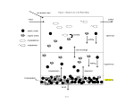 Figure 3. Equilibrium Partitioning of Mercury to Solids and DOC
-Hgll
:- Hgll
- Hgll«
abio.Hgll
Hgll
DOC,HgII
DOC-'Hgll
MeHg-i
MeHg -:
MeHg -c
- /v| I
MeHg -DOC
abiotic
organic
phytoplankto
/\-( | zooplankton
DOC dissolved organic carbon
F-2
image:
Figure 3. Equilibrium Partitioning of Mercury to Solids and DOC
-Hgll
:- Hgll
- Hgll«
abio.Hgll
Hgll
DOC,HgII
DOC-'Hgll
MeHg-i
MeHg -:
MeHg -c
- /v| I
MeHg -DOC
abiotic
organic
phytoplankto
/\-( | zooplankton
DOC dissolved organic carbon
F-2
image:
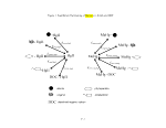 Figure 4. Mercury Loading to the Water Body (Atmospheric and Watershed)
Gaseous
Diffusion
Wet Deposition = Precipitation x Hg Cone, in Precipitation
I
Atmospheric Loading = Dry Deposition + Wet Deposition
% Known
Contaminated
Soils
Yo Riparian
% Wetlands
Water Body
F-4
image:
Figure 4. Mercury Loading to the Water Body (Atmospheric and Watershed)
Gaseous
Diffusion
Wet Deposition = Precipitation x Hg Cone, in Precipitation
I
Atmospheric Loading = Dry Deposition + Wet Deposition
% Known
Contaminated
Soils
Yo Riparian
% Wetlands
Water Body
F-4
image:
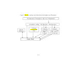 Figure 5. Mercury Fate Process Formulation in the Water Body
N^Vwatershed loading
X^
\
inflow
r-
rA
^*x^
1 ,^> HaO
U
*— '
r
s
photo-
gaseous
evasion
atmospheric r-.j
deposition (- J photo-lytic
r_j oxidation
(-J and reduction
r-J
J V <-'
^ reduction
^ _.
outflow
I-—
1 "!>
oxidation _H§n
y^ «
x
N demethylatioj? /
\ / /
demethylation \ / /
/ /methylation |-|
m (UK/
cr>
MeHg »•
* partitioning complexation
A tosohds with DOC
resuspension
U n H
J L hiirial
settling
V
dispersion A
aemetnyiation
TT ^- A /T TT
c? ^ r c?
^
methvlation
(1
u-^
sediments
V
F-5
image:
Figure 5. Mercury Fate Process Formulation in the Water Body
N^Vwatershed loading
X^
\
inflow
r-
rA
^*x^
1 ,^> HaO
U
*— '
r
s
photo-
gaseous
evasion
atmospheric r-.j
deposition (- J photo-lytic
r_j oxidation
(-J and reduction
r-J
J V <-'
^ reduction
^ _.
outflow
I-—
1 "!>
oxidation _H§n
y^ «
x
N demethylatioj? /
\ / /
demethylation \ / /
/ /methylation |-|
m (UK/
cr>
MeHg »•
* partitioning complexation
A tosohds with DOC
resuspension
U n H
J L hiirial
settling
V
dispersion A
aemetnyiation
TT ^- A /T TT
c? ^ r c?
^
methvlation
(1
u-^
sediments
V
F-5
image:
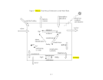 APPENDIX
Literature Mercury Process Rate Constants
image:
APPENDIX
Literature Mercury Process Rate Constants
image:
 Default Rate Constants of Mercury Transformation Processes
Process
Methylation
Demethylation
Biotic Reduction
Photo-Degradation (MeHg --> HgO)
Photo-Reduction (Hgll -> HgO) Visible Light
Photo-Reduction (Hgll -> HgO) UV-B
Photo-Oxidation (HgO -> Hgll) UV-B
Dark Oxidation
Trophic Level 1 BAF: Phytoplankton
Trophic Level 2 BAF: Zooplankton
Trophic Level 2 BAF: Benthos
Trophic Level 3 BAF: Fish
Trophic Level 4 BAF: Fish
Media
Epilimnion
Hypolimnion
Sediment
Epilimnion
Hypolimnion
Sediment
Water Column
Water Column
Water Column
Water Column
Water Column
Water Column
Phyto
Zoo
Benthos
Fish
Fish
Value
0.001
0.001
0.001
0.0001
0.001
0.002
0.03
0.002
0.03
28.25
58.85
1.44
4.94E+05
1.61E+06
2.48E+06
1.60E+06
6.80E+06
Units
per day
per day
per day
per day
per day
per day
per day
per day per
E/m2-day
per day per
E/m2-day
per day per
E/m2-day
per day per
E/m2-day
per day
(ug/kg)/(ug/L)
(ug/kg)/(ug/L)
(ug/kg)/(ug/L)
(ug/kg)/(ug/L)
(ug/kg)/(ug/L)
A-l
image:
Default Rate Constants of Mercury Transformation Processes
Process
Methylation
Demethylation
Biotic Reduction
Photo-Degradation (MeHg --> HgO)
Photo-Reduction (Hgll -> HgO) Visible Light
Photo-Reduction (Hgll -> HgO) UV-B
Photo-Oxidation (HgO -> Hgll) UV-B
Dark Oxidation
Trophic Level 1 BAF: Phytoplankton
Trophic Level 2 BAF: Zooplankton
Trophic Level 2 BAF: Benthos
Trophic Level 3 BAF: Fish
Trophic Level 4 BAF: Fish
Media
Epilimnion
Hypolimnion
Sediment
Epilimnion
Hypolimnion
Sediment
Water Column
Water Column
Water Column
Water Column
Water Column
Water Column
Phyto
Zoo
Benthos
Fish
Fish
Value
0.001
0.001
0.001
0.0001
0.001
0.002
0.03
0.002
0.03
28.25
58.85
1.44
4.94E+05
1.61E+06
2.48E+06
1.60E+06
6.80E+06
Units
per day
per day
per day
per day
per day
per day
per day
per day per
E/m2-day
per day per
E/m2-day
per day per
E/m2-day
per day per
E/m2-day
per day
(ug/kg)/(ug/L)
(ug/kg)/(ug/L)
(ug/kg)/(ug/L)
(ug/kg)/(ug/L)
(ug/kg)/(ug/L)
A-l
image:
 Mercury Process Rate Constants
From Mercury Report to Congress
Rate Constants, day *
Volatilization of Hg
Oxidation
Reduction
Methylation
Demethylation of Hgll
Mer demethylation to Hg°
Watershed Soil, day *
0.082
0
0.000025
0.00005
0.0025
0
Water Column, day *
0.10
0
0.0075
0.001
0.015
0
Benthic Sediments, day *
0
0
0.000001
0.0001
0.002
0
A-2
image:
Mercury Process Rate Constants
From Mercury Report to Congress
Rate Constants, day *
Volatilization of Hg
Oxidation
Reduction
Methylation
Demethylation of Hgll
Mer demethylation to Hg°
Watershed Soil, day *
0.082
0
0.000025
0.00005
0.0025
0
Water Column, day *
0.10
0
0.0075
0.001
0.015
0
Benthic Sediments, day *
0
0
0.000001
0.0001
0.002
0
A-2
image:
 Methylation in Water Column: Hgll -^ MeHg
Process
Abiotic
Methylation
Epilimnetic
Methylation
Methylation
Potential
Methylation
Methylation
Methylation
Methylation
Methylation
Methylation
Methylation
Rates
0.000024 - 0.00124 d'1, peak in
summer, yearly average ~
.00033 d'1 *
0.000005 L/mgDOC/day
0.001 d'1
0.0001 -0.003d'1
0.0001- 0.0014 d'1 or
0.67- 9.38 ng/L/d
0.0003-0.0031 d~l or
2.01 -20.77 ng/L/d
< 0.0005 d'1 or
< 33 ng/L/d
0
0.003 ng/L/d (3m, 4.4 mg/L
DO), 0.03 ng/L/d (9m, 0.9
mg/L DO)), 0. 1 1 ng/L/d (15m)
0.0001 -0.003 per day
Notes
Methylation in aerobic waters was abiotic;
was suppressed by color and particulates;
increase with T, pH, decrease with color
Default Rate in R-MCM, for Epilimnion
Mercury Report to Congress
Maximum potential methylation rate, as
summarized in Mercury Report to
Congress
pH 6.0 - 8.3, EL A Lakes, ON, oligo to
eutrotrophic lakes
pH 5.3 - 5.9 ELA Lakes, ON, oligo to
eutrophic lakes
pH 6.5, small oligotrophic lake, Lake
Clara, WI
Impounded lake, Southern Indian Lake,
MB
Net MeHg production rates increased with
depth/decreasing DO; alkaline,
hypereutrophic lake (Onondaga Lake,
NY). Low transparency, pH 7.5.
Lab Spiked Experiments
References
Matilainen and Verta, 1995. l
R-MCM. 2
Mercury Report to Congress.
Gilmour and Henry, 1991.
Xun, etal, 1987. 5
Xun, etal, 1987.
Korthals & Winfrey, 1987. 6
Ramlaletal. 19877
Henry etal, 1995.8
Xun et al., 1987; Korthals and
Winfrey, 1987; Gilmour and
Henry, 1990, as cited in Fitzgerald,
etal., 1994. 9
* yearly average calculated as V* of summer average. This average comes from assuming a relatively sinusoidal annual pattern of
a max in the summer going to almost zero in the winter, and around half in the spring and fall.
A-2
image:
Methylation in Water Column: Hgll -^ MeHg
Process
Abiotic
Methylation
Epilimnetic
Methylation
Methylation
Potential
Methylation
Methylation
Methylation
Methylation
Methylation
Methylation
Methylation
Rates
0.000024 - 0.00124 d'1, peak in
summer, yearly average ~
.00033 d'1 *
0.000005 L/mgDOC/day
0.001 d'1
0.0001 -0.003d'1
0.0001- 0.0014 d'1 or
0.67- 9.38 ng/L/d
0.0003-0.0031 d~l or
2.01 -20.77 ng/L/d
< 0.0005 d'1 or
< 33 ng/L/d
0
0.003 ng/L/d (3m, 4.4 mg/L
DO), 0.03 ng/L/d (9m, 0.9
mg/L DO)), 0. 1 1 ng/L/d (15m)
0.0001 -0.003 per day
Notes
Methylation in aerobic waters was abiotic;
was suppressed by color and particulates;
increase with T, pH, decrease with color
Default Rate in R-MCM, for Epilimnion
Mercury Report to Congress
Maximum potential methylation rate, as
summarized in Mercury Report to
Congress
pH 6.0 - 8.3, EL A Lakes, ON, oligo to
eutrotrophic lakes
pH 5.3 - 5.9 ELA Lakes, ON, oligo to
eutrophic lakes
pH 6.5, small oligotrophic lake, Lake
Clara, WI
Impounded lake, Southern Indian Lake,
MB
Net MeHg production rates increased with
depth/decreasing DO; alkaline,
hypereutrophic lake (Onondaga Lake,
NY). Low transparency, pH 7.5.
Lab Spiked Experiments
References
Matilainen and Verta, 1995. l
R-MCM. 2
Mercury Report to Congress.
Gilmour and Henry, 1991.
Xun, etal, 1987. 5
Xun, etal, 1987.
Korthals & Winfrey, 1987. 6
Ramlaletal. 19877
Henry etal, 1995.8
Xun et al., 1987; Korthals and
Winfrey, 1987; Gilmour and
Henry, 1990, as cited in Fitzgerald,
etal., 1994. 9
* yearly average calculated as V* of summer average. This average comes from assuming a relatively sinusoidal annual pattern of
a max in the summer going to almost zero in the winter, and around half in the spring and fall.
A-2
image:
 Photodegradation of MeHg in water column: MeHg -> HgO
Process
Photodegradation of
MeHg
Photo-Reduction
Photo-Reduction
Reduction
Reduction
Medium
Water
Column
Water
Column
Water
Column
Water
Column
Water
Column
Chemistry
Hgll/HgO
Hgll-
Hgll-
Hgll-
Hgll-
>HgO
>HgO
>HgO
>HgO
Rates
0.002*PAR d'1,
PAR = E/m2/d
DGM Production
[fM/h]=
0.289 +0.2(PAR) -
5.02e-5(PAR)2
0.005-0.1 d'1
0.1 d" (summer, 3 m);
0.05 d"1 (summer, 9 m);
0.22 d'1 (May, 6m)
Notes
Two figures, k = 0.0022*PAR
andk = 0.0019*PAR.
For six dates: 3 in Aug, 1 in
Sept, 2 in Nov. PAR in kJ/m2/h
Photo-reduction under UV light
in tropical waters showed that
filtration had no effect on
photoreduction, particulates
favor the reaction under
anaerobic conditions, C>2 and
N2 had no effect on reaction.
Reduction rates in equatorial
Pacific and Wisconsin lakes
Reduction Rates at Palette
Lake
References
Sellers etal. 1996.
Amy ot etal. 1994.
Beucher et al., 2002
Mason, etal. 1994
Vandal etal. 1995.
10
11
12
13
14
A-4
image:
Photodegradation of MeHg in water column: MeHg -> HgO
Process
Photodegradation of
MeHg
Photo-Reduction
Photo-Reduction
Reduction
Reduction
Medium
Water
Column
Water
Column
Water
Column
Water
Column
Water
Column
Chemistry
Hgll/HgO
Hgll-
Hgll-
Hgll-
Hgll-
>HgO
>HgO
>HgO
>HgO
Rates
0.002*PAR d'1,
PAR = E/m2/d
DGM Production
[fM/h]=
0.289 +0.2(PAR) -
5.02e-5(PAR)2
0.005-0.1 d'1
0.1 d" (summer, 3 m);
0.05 d"1 (summer, 9 m);
0.22 d'1 (May, 6m)
Notes
Two figures, k = 0.0022*PAR
andk = 0.0019*PAR.
For six dates: 3 in Aug, 1 in
Sept, 2 in Nov. PAR in kJ/m2/h
Photo-reduction under UV light
in tropical waters showed that
filtration had no effect on
photoreduction, particulates
favor the reaction under
anaerobic conditions, C>2 and
N2 had no effect on reaction.
Reduction rates in equatorial
Pacific and Wisconsin lakes
Reduction Rates at Palette
Lake
References
Sellers etal. 1996.
Amy ot etal. 1994.
Beucher et al., 2002
Mason, etal. 1994
Vandal etal. 1995.
10
11
12
13
14
A-4
image:
 Photo-Oxidation in Water Column: HgO -> Hgll
Process
Photo-Oxidation
Dark Oxidation
Redox
Medium
Water
Column
Water
Column
Water
Column
Chemistry
HgO ^ Hgll
HgO ^ Hgll
HgO ^ Hgll
vs Hgll -»
Hgo
Rates
0.25 ± 0.02 hr1 per 5.5
uE/m2/s, DOC 3. 5 -4.3
mg C/L, Cr4 7 _ 5 3 e-
4M.
0.06 hr" , pseudo-first
order
Notes
Lab showed oxidation of HgO
requires, Cl", a photoreactive
compound (e.g., quinine), light.
In Natural waters, Cl° was not
needed.
Oxidation of HgO in saline
water in dark
Amyot compares his reduction
rates to oxidation rates and
believes they are of similar
value because the oxidation
rates were done at 1/10 the
intensity of incident UV
radiation
References
LaLonde, etal., 2001.
15
LaLonde, et al, 2000.
LaLonde, et al., 2000
A-5
image:
Photo-Oxidation in Water Column: HgO -> Hgll
Process
Photo-Oxidation
Dark Oxidation
Redox
Medium
Water
Column
Water
Column
Water
Column
Chemistry
HgO ^ Hgll
HgO ^ Hgll
HgO ^ Hgll
vs Hgll -»
Hgo
Rates
0.25 ± 0.02 hr1 per 5.5
uE/m2/s, DOC 3. 5 -4.3
mg C/L, Cr4 7 _ 5 3 e-
4M.
0.06 hr" , pseudo-first
order
Notes
Lab showed oxidation of HgO
requires, Cl", a photoreactive
compound (e.g., quinine), light.
In Natural waters, Cl° was not
needed.
Oxidation of HgO in saline
water in dark
Amyot compares his reduction
rates to oxidation rates and
believes they are of similar
value because the oxidation
rates were done at 1/10 the
intensity of incident UV
radiation
References
LaLonde, etal., 2001.
15
LaLonde, et al, 2000.
LaLonde, et al., 2000
A-5
image:
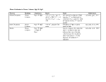 Demethylation in Water Column: MeHg -> Hgll
Process
Biotic
Demethylation
Demethylation
Demethylation
Demethylation
Demethylation
Potential
Demethylation
Medium
Water
Column
Water
Column
Water
Column
Water
Column
Water
Column
Water
Column
Chemistry
MeHg-
MeHg-
MeHg-
MeHg-
MeHg-
MeHg-
>HgII
>HgII
>HgII
>HgII
>HgII
>HgII
Rates
<0.001 to 0.132 d'1,
peak in summer,
summer avg 0.0835 d"1,
-0.021 yearly avg*
0.0020- 0.00254 d'1
0.0021-0.0238 d'1
0.001-0.005 d'1
0.015 d'1
0.001- 0.025 d'1
Notes
Experiments in dark, sterilized
&/or filtered showed no
demethylation: biotic; rates
increased with T and organic
matter
pH 6.0 - 8.3, ELA Lakes, ON,
oligo to eutrotrophic lakes
pH 5. 3 -5. 9 EL A Lakes, ON,
oligo to eutrophic lakes
pH6.5
Mercury Report to Congress
Maximum potential
demethylation rate, as
summarized in Mercury Report
to Congress
References
Matilainen and Verta,
1995.
Xun, etal, 1987.
Xun, etal, 1987.
Korthals & Winfrey,
1987,
Mercury Report to
Congress.
Gilmour and Henry,
1991.
A-6
image:
Demethylation in Water Column: MeHg -> Hgll
Process
Biotic
Demethylation
Demethylation
Demethylation
Demethylation
Demethylation
Potential
Demethylation
Medium
Water
Column
Water
Column
Water
Column
Water
Column
Water
Column
Water
Column
Chemistry
MeHg-
MeHg-
MeHg-
MeHg-
MeHg-
MeHg-
>HgII
>HgII
>HgII
>HgII
>HgII
>HgII
Rates
<0.001 to 0.132 d'1,
peak in summer,
summer avg 0.0835 d"1,
-0.021 yearly avg*
0.0020- 0.00254 d'1
0.0021-0.0238 d'1
0.001-0.005 d'1
0.015 d'1
0.001- 0.025 d'1
Notes
Experiments in dark, sterilized
&/or filtered showed no
demethylation: biotic; rates
increased with T and organic
matter
pH 6.0 - 8.3, ELA Lakes, ON,
oligo to eutrotrophic lakes
pH 5. 3 -5. 9 EL A Lakes, ON,
oligo to eutrophic lakes
pH6.5
Mercury Report to Congress
Maximum potential
demethylation rate, as
summarized in Mercury Report
to Congress
References
Matilainen and Verta,
1995.
Xun, etal, 1987.
Xun, etal, 1987.
Korthals & Winfrey,
1987,
Mercury Report to
Congress.
Gilmour and Henry,
1991.
A-6
image:
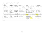 Reduction in Water Column: Hgll -> HgO
Process
Abiotic Reduction
Reduction
Abiotic reduction
Ice Over HgO
HgO
F ormati on/Reducti on
HgO
F ormati on/Reducti on
Medium
Water
Column
Water
Column
Water
Column
Water
Column
Water
Column
Chemistry Rates
Hgll ^ HgO 0.011 per day
Hgll -» HgO 0.0028 -0.07 d'1 (max
depth 10.3 m; 9.8 ha;
pH 4.7; ALK -7 ueq/L;
2.6 mgDOC/L); 0.012-
0.28 d"1 (max depth 18.2
m; 70 ha; pH 7.25; ALK
128 ueq/L; 5.06 mg
DOC/L)
Hgll -» HgO 0.22 d'1
Hgll -» HgO
Hgll -» HgO Conversion rates of 0.02
-0.04 d'1
Notes
Abiotic formation rates for
dH2O, dH2O with trace metals,
and microwaved mystic
lakewater
Using observed evasion rates,
these HgO formation rates were
estimated for two years (1989
and 1990) for two lakes with
given characteristics
Laboratory presented abiotic
production rate of HgO in the
presence of humid acids
In Wisconsin lakes, no
significant increase in [HgO]
during winter ice over
Strong positive correlation
between pH and HgO
formation, with supersaturation
of HgO between up to 12 times
that of saturation concentration
required to balance estimated
evasional fluxes of 200-400
pml/m2/d
References
Mason etal., 1995. 16
Fitzgerald et al., 1994.
Alberts et al., 1974 as
cited by Fitzgerald et
al., 1994.
Personal
communication with
G.M. Vandal as cited
by Fitzgerald et al.,
1994.
Vandal, et al., 1991. 17
Mason et al., 1995.
A-7
image:
Reduction in Water Column: Hgll -> HgO
Process
Abiotic Reduction
Reduction
Abiotic reduction
Ice Over HgO
HgO
F ormati on/Reducti on
HgO
F ormati on/Reducti on
Medium
Water
Column
Water
Column
Water
Column
Water
Column
Water
Column
Chemistry Rates
Hgll ^ HgO 0.011 per day
Hgll -» HgO 0.0028 -0.07 d'1 (max
depth 10.3 m; 9.8 ha;
pH 4.7; ALK -7 ueq/L;
2.6 mgDOC/L); 0.012-
0.28 d"1 (max depth 18.2
m; 70 ha; pH 7.25; ALK
128 ueq/L; 5.06 mg
DOC/L)
Hgll -» HgO 0.22 d'1
Hgll -» HgO
Hgll -» HgO Conversion rates of 0.02
-0.04 d'1
Notes
Abiotic formation rates for
dH2O, dH2O with trace metals,
and microwaved mystic
lakewater
Using observed evasion rates,
these HgO formation rates were
estimated for two years (1989
and 1990) for two lakes with
given characteristics
Laboratory presented abiotic
production rate of HgO in the
presence of humid acids
In Wisconsin lakes, no
significant increase in [HgO]
during winter ice over
Strong positive correlation
between pH and HgO
formation, with supersaturation
of HgO between up to 12 times
that of saturation concentration
required to balance estimated
evasional fluxes of 200-400
pml/m2/d
References
Mason etal., 1995. 16
Fitzgerald et al., 1994.
Alberts et al., 1974 as
cited by Fitzgerald et
al., 1994.
Personal
communication with
G.M. Vandal as cited
by Fitzgerald et al.,
1994.
Vandal, et al., 1991. 17
Mason et al., 1995.
A-7
image:
 Reduction
Biotic Reduction
Reduction
Reduction
Water
Column
Water
Column
Water
Column
Water
Column
Water
Column
Hgll -» HgO <0.005 to 0.079 d'1
Hgll -» HgO
Hgll -» HgO
Hgll ^ HgO 0.038 d'1 (1m), 031 d'1,
(5m), .Old'1 (7m), .011
d'1 (9m), <0.005 d'1
(19m)
Hgll -» HgO 0.05 - 0.3 d'1; low DOC
(l.l-2.3mg/L): 0.2-
0.4 d'1, high DOC (5.0-
8.7 mg/L): 0.02-0.2 d'1
Range of rates from Apr to Mason et al., 1995.
Nov '93 for Upper Mystic
Lake, Boston. Rates highest in
April, July, and Oct., low in
June and Nov
Correlation between chl a and Mason et al., 1995.
HgO formation rate,
Argue that reduction in natural Mason et al., 1995.
waters primarily by small
organisms (<3um diam).
HgO production decreased with Mason et al., 1995.
Depth
Volatile mercury percent Amyot, et al. 1997. 18
formation in arctic lakes, UV
penetrates deeper in low DOC
lakes suggesting higher rates
correlated with light
penetration.
A-8
image:
Reduction
Reduction
Biotic Reduction
Reduction
Reduction
Water
Column
Water
Column
Water
Column
Water
Column
Water
Column
Hgll -» HgO <0.005 to 0.079 d'1
Hgll -» HgO
Hgll -» HgO
Hgll ^ HgO 0.038 d'1 (1m), 031 d'1,
(5m), .Old'1 (7m), .011
d'1 (9m), <0.005 d'1
(19m)
Hgll -» HgO 0.05 - 0.3 d'1; low DOC
(l.l-2.3mg/L): 0.2-
0.4 d'1, high DOC (5.0-
8.7 mg/L): 0.02-0.2 d'1
Range of rates from Apr to Mason et al., 1995.
Nov '93 for Upper Mystic
Lake, Boston. Rates highest in
April, July, and Oct., low in
June and Nov
Correlation between chl a and Mason et al., 1995.
HgO formation rate,
Argue that reduction in natural Mason et al., 1995.
waters primarily by small
organisms (<3um diam).
HgO production decreased with Mason et al., 1995.
Depth
Volatile mercury percent Amyot, et al. 1997. 18
formation in arctic lakes, UV
penetrates deeper in low DOC
lakes suggesting higher rates
correlated with light
penetration.
A-8
image:
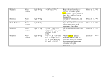 Methyl Mercury in Sediments
Process
MethylMercury
Methylation
Methylation
Methylation
Methylation
Methylation
Methylation
Methylation
Methylation
Medium
Sediments
Sediments
Sediments
Sediments
Sediments
Sediments
Sediments
Sediments
Sediments
Chemistry
MeHg
Hgn-»
Hgll^
Hgn-»
Hgll^
Hgll^
Hgll^
Hgll^
Hgll^
MeHg
MeHg
MeHg
MeHg
MeHg
MeHg
MeHg
MeHg
Rates Notes
Typical %MeHg
1 - 1 5%
0 006 7e-5 2 5e-5 d "^ Gross methylation rates
2.25 - 8.75 ug/m3/d
(avg: 5.92)
0.0001 d" Mercury Report to Congress
0.8 -96 ng/g/d or
0.0004 - 0.048 d'1 for
pH 6-7 (epi) in slurries;
or for pH 4-5: 0-38
ng/g/d or 0.002 -
0.0019 d'1
0.03 -1.9 ng/g/d;
0.0005- 0.028 d'1
0.3 - 2.3 ng/g/d;
0.45- 0.0017 d'1
0.5 ng/g/d or <0.001 d'1
(LOI<1%), 1.5 ng/g/d
or 0.015 d'1 (LOT 60%);
6 ng/g/d or 0.0005 d'1
0 - 62.4 ng/g/d or 0 -
0.0312 d'1; 0-148
ng/g/d or 0 - 0.0744 d'1
References
Ulrichetal., 2001 iy
Gilmour and Riedel,
1995.20
Mercury Report to
Congress
Ramlaletal., 1985
cited by Gilmour and
Henry, 1991.
Korthals & Winfrey,
1987, as cited by
Gilmour and Henry,
1991
Steffanetal. 1988. as
cited by Gilmour and
Henry, 1991.
Kudoetal. 1977. as
cited by Gilmour and
Henry, 1991.
Spangler et al. 1973 as
cited by Gilmour and
Henry, 1991.
Ramlaletal, 1987 as
cited by Gilmour and
Henry, 1991.
A-9
image:
Methyl Mercury in Sediments
Process
MethylMercury
Methylation
Methylation
Methylation
Methylation
Methylation
Methylation
Methylation
Methylation
Medium
Sediments
Sediments
Sediments
Sediments
Sediments
Sediments
Sediments
Sediments
Sediments
Chemistry
MeHg
Hgn-»
Hgll^
Hgn-»
Hgll^
Hgll^
Hgll^
Hgll^
Hgll^
MeHg
MeHg
MeHg
MeHg
MeHg
MeHg
MeHg
MeHg
Rates Notes
Typical %MeHg
1 - 1 5%
0 006 7e-5 2 5e-5 d "^ Gross methylation rates
2.25 - 8.75 ug/m3/d
(avg: 5.92)
0.0001 d" Mercury Report to Congress
0.8 -96 ng/g/d or
0.0004 - 0.048 d'1 for
pH 6-7 (epi) in slurries;
or for pH 4-5: 0-38
ng/g/d or 0.002 -
0.0019 d'1
0.03 -1.9 ng/g/d;
0.0005- 0.028 d'1
0.3 - 2.3 ng/g/d;
0.45- 0.0017 d'1
0.5 ng/g/d or <0.001 d'1
(LOI<1%), 1.5 ng/g/d
or 0.015 d'1 (LOT 60%);
6 ng/g/d or 0.0005 d'1
0 - 62.4 ng/g/d or 0 -
0.0312 d'1; 0-148
ng/g/d or 0 - 0.0744 d'1
References
Ulrichetal., 2001 iy
Gilmour and Riedel,
1995.20
Mercury Report to
Congress
Ramlaletal., 1985
cited by Gilmour and
Henry, 1991.
Korthals & Winfrey,
1987, as cited by
Gilmour and Henry,
1991
Steffanetal. 1988. as
cited by Gilmour and
Henry, 1991.
Kudoetal. 1977. as
cited by Gilmour and
Henry, 1991.
Spangler et al. 1973 as
cited by Gilmour and
Henry, 1991.
Ramlaletal, 1987 as
cited by Gilmour and
Henry, 1991.
A-9
image:
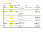 Methylation
Methylation
Methylation
Methylation
Sediments Hgll -> MeHg
Sediments Hgll -> MeHg
Sediments Hgll -> MeHg
Sediments Hgll -> MeHg
Sediments Hgll -> MeHg
1-9 ng/g/d; 0.0009-
0.01 d'1
0.05 -3.0 ng/g/d or
0.00001 -0.0003d'1;
0.19 -3. 85 ng/g/d or
0.00038- 0.0077 d'1
0.8 -6. 8 ng/g/d or 0.02
- 0. 17 d'1; and 2.8 -4
ng/g/d or 0.07 -0.1 d'1
0.001- 0.016 d'1
0.0006- 0.18 d'1
Jensen and Jernelov,
1969 as cited by
Gilmour and Henry,
1991.
Gilmour and Mitchell
1988(a,b), Gilmour et
al, ?? as cited by
Gilmour and Henry,
1991.
Jackson. 1989. as cited
by Gilmour and Henry,
1991.
Hintelmann et al.
200021 and references
therein
Stordal and Gill,
1995.22
A-10
image:
Methylation
Methylation
Methylation
Methylation
Methylation
Sediments Hgll -> MeHg
Sediments Hgll -> MeHg
Sediments Hgll -> MeHg
Sediments Hgll -> MeHg
Sediments Hgll -> MeHg
1-9 ng/g/d; 0.0009-
0.01 d'1
0.05 -3.0 ng/g/d or
0.00001 -0.0003d'1;
0.19 -3. 85 ng/g/d or
0.00038- 0.0077 d'1
0.8 -6. 8 ng/g/d or 0.02
- 0. 17 d'1; and 2.8 -4
ng/g/d or 0.07 -0.1 d'1
0.001- 0.016 d'1
0.0006- 0.18 d'1
Jensen and Jernelov,
1969 as cited by
Gilmour and Henry,
1991.
Gilmour and Mitchell
1988(a,b), Gilmour et
al, ?? as cited by
Gilmour and Henry,
1991.
Jackson. 1989. as cited
by Gilmour and Henry,
1991.
Hintelmann et al.
200021 and references
therein
Stordal and Gill,
1995.22
A-10
image:
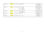 Demethylation in Sediments: MeHg -^ Hgll
Rates Notes
0.002- 0.0254 d'1;
00021 -00238H"1
0.001 -O.OOSd'1;
0.003- 0.062 d'1
0.015 d'1
0.037- 0.137 d'1;
001 H"1
0.038- 0.074 d'1;
0.0048- 0.065 d'1
0.001 d'1
0.0005 -0.0043d'1;
0.0002- 0.00025 d'1
0.390- 0.528 d'1
References
Xun et al. 1987, as cited by Gilmour and Henry, 1991.
Korthals and Winfrey, 1987, as cited by Gilmour and
Henry, 1991.
Steffan et al. 1988, as cited by Gilmour and Henry,
1991.
Kudo et al. 1977, as cited by Gilmour and Henry, 1991.
Ramlal et al. 1987, as cited by Gilmour and Henry,
1991.
Jensen and Jernelov, 1969, as cited by Gilmour and
Henry, 1991.
Jackson. 1989, as cited by Gilmour and Henry, 1991.
Hintelmann et al., 2000.
A-ll
image:
Demethylation in Sediments: MeHg -^ Hgll
Rates Notes
0.002- 0.0254 d'1;
00021 -00238H"1
0.001 -O.OOSd'1;
0.003- 0.062 d'1
0.015 d'1
0.037- 0.137 d'1;
001 H"1
0.038- 0.074 d'1;
0.0048- 0.065 d'1
0.001 d'1
0.0005 -0.0043d'1;
0.0002- 0.00025 d'1
0.390- 0.528 d'1
References
Xun et al. 1987, as cited by Gilmour and Henry, 1991.
Korthals and Winfrey, 1987, as cited by Gilmour and
Henry, 1991.
Steffan et al. 1988, as cited by Gilmour and Henry,
1991.
Kudo et al. 1977, as cited by Gilmour and Henry, 1991.
Ramlal et al. 1987, as cited by Gilmour and Henry,
1991.
Jensen and Jernelov, 1969, as cited by Gilmour and
Henry, 1991.
Jackson. 1989, as cited by Gilmour and Henry, 1991.
Hintelmann et al., 2000.
A-ll
image:
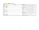 Reduction in Sediments: Hgll -> HgO
Notes References
At cone, of 65 pg/L HgO, or 10% HgT as HgO Vandal, et al. 1995.
A-12
image:
Reduction in Sediments: Hgll -> HgO
Notes References
At cone, of 65 pg/L HgO, or 10% HgT as HgO Vandal, et al. 1995.
A-12
image:
 REFERENCES
1 Matilainen, T., Verta, M. 1995. Mercury Methylation and Demethylation in Aerobic Surface Waters. Can. J. Fish Aquat. Sci. 52.
1597-1608.
2R-MCM
3 Mercury Report to Congress
4 Gilmour, C.C. and E.A. Henry (1991). Mercury Methylation in Aquatic Systems Affected by Acid
Deposition. Environmental Pollution, 71:131-169.
5 Xun, L., N Campbell, J. Rudd. 1987. Measurements of Specific Rates of Net Methyl Mercury Production in the Water Column and
Surface Sediments of Acidified and Circumneutral Lakes. 44 (4): 750-757.
6 Korthals, E.T., Winfrey, M.R., 1987. Seasonal and Spatial Variations in Mercury Methylation and Demethylation in an Oligotrophic
Lake. Appl. Environ. Microbiol. 53, 2397-2404.
7 Ramlal, P.S., C. Anema, A. Furutani, R.E. Hecky, J.W.M. Rudd. 1987. Mercury Methylation and Demethylation Studies in Southern
Indian Lake, Manitoba. Can Tech Rep Fish Aquat Sci, 1490 v + 35p.
8 Henry, E.A., LJ. Dodge-Murphy, G.N. Bigham, S.M. Klein, C.C. Gilmour. 1995. Total Mercury and Methylmercury Mass Balance
in an Alakline, Hypereutrophic Urban Lake (Onondaga Lake, NY). Water, Air, and Soil Pollution. 80: 509-518, 1995.
9 Fitzgerald, W.F., R.P. Mason, G.M. Vandal, F. Dulac. 1994. Air-Water Cycling of Mercury in Lakes. In Mercury Pollution:
Integration and Synthesis. Ed. C. J. Watras and J.W. Huckabee. Lewis Publishers, Boca Raton.
10 Sellers, P., C.A. Kelly, J.W.M Rudd, A.R. MacHutcheon. 1996. Photodegradation of Methylmercury in Lakes. Nature. 380: 694 -
697. April.
11 Amyot, M. G. Mierle, D.R.S. Lean, DJ. McQueen. 1994. Sunlight-Induced Formation of Dissolved Gaseous Mercury in Lake
Waters. Environmental Science & Technology. 28: 2366-2371.
12 Beucher, C., P. Wong-Wah-Chung, C. Richard, G. Mailhot, M. Bolte, D. Cossa. 2002. Dissolved Gaseous Mercury Formation
Under UV Irradiation of Unam ended Tropical Waters from French Guyana. The Science of the Total Environment. 290: 131-138.
13 Mason, R.P. Fitzgerald, W.F., F.M.M.Morel. 1994. The Biogeochemical Cycling of Elemental Mercury: Anthropogenic Influences.
Geochimica et Cosmochimica Acta. 58(15):3191-3198.
14 Vandal, G.M., W.F. Fitzgerald, K.R. Rolfhus, and C.H. Lamborg. 1995. Modeling the Elemental Mercury Cycle in Pallette Lake,
Wisconsin, USA. Water, Air, and Soil Pollution. 80: 789-798.
15 LaLonde, J.D., M. Amyot, A.M.L. Morel, F.M.M. Morel. 2001. Photooxidation of Hg(0) in Artificial and Natural Waters. Environ.
Sci. Technol. 35: 1367-1372.
16 Mason, R.P., F.M.M. Morel, H.F. Hemond. 1995. The Role of Microorganisms in Elemental Mercury Formation in Natural Waters.
Water, Air and Soil Pollution. 80: 775-787.
A-13
image:
REFERENCES
1 Matilainen, T., Verta, M. 1995. Mercury Methylation and Demethylation in Aerobic Surface Waters. Can. J. Fish Aquat. Sci. 52.
1597-1608.
2R-MCM
3 Mercury Report to Congress
4 Gilmour, C.C. and E.A. Henry (1991). Mercury Methylation in Aquatic Systems Affected by Acid
Deposition. Environmental Pollution, 71:131-169.
5 Xun, L., N Campbell, J. Rudd. 1987. Measurements of Specific Rates of Net Methyl Mercury Production in the Water Column and
Surface Sediments of Acidified and Circumneutral Lakes. 44 (4): 750-757.
6 Korthals, E.T., Winfrey, M.R., 1987. Seasonal and Spatial Variations in Mercury Methylation and Demethylation in an Oligotrophic
Lake. Appl. Environ. Microbiol. 53, 2397-2404.
7 Ramlal, P.S., C. Anema, A. Furutani, R.E. Hecky, J.W.M. Rudd. 1987. Mercury Methylation and Demethylation Studies in Southern
Indian Lake, Manitoba. Can Tech Rep Fish Aquat Sci, 1490 v + 35p.
8 Henry, E.A., LJ. Dodge-Murphy, G.N. Bigham, S.M. Klein, C.C. Gilmour. 1995. Total Mercury and Methylmercury Mass Balance
in an Alakline, Hypereutrophic Urban Lake (Onondaga Lake, NY). Water, Air, and Soil Pollution. 80: 509-518, 1995.
9 Fitzgerald, W.F., R.P. Mason, G.M. Vandal, F. Dulac. 1994. Air-Water Cycling of Mercury in Lakes. In Mercury Pollution:
Integration and Synthesis. Ed. C. J. Watras and J.W. Huckabee. Lewis Publishers, Boca Raton.
10 Sellers, P., C.A. Kelly, J.W.M Rudd, A.R. MacHutcheon. 1996. Photodegradation of Methylmercury in Lakes. Nature. 380: 694 -
697. April.
11 Amyot, M. G. Mierle, D.R.S. Lean, DJ. McQueen. 1994. Sunlight-Induced Formation of Dissolved Gaseous Mercury in Lake
Waters. Environmental Science & Technology. 28: 2366-2371.
12 Beucher, C., P. Wong-Wah-Chung, C. Richard, G. Mailhot, M. Bolte, D. Cossa. 2002. Dissolved Gaseous Mercury Formation
Under UV Irradiation of Unam ended Tropical Waters from French Guyana. The Science of the Total Environment. 290: 131-138.
13 Mason, R.P. Fitzgerald, W.F., F.M.M.Morel. 1994. The Biogeochemical Cycling of Elemental Mercury: Anthropogenic Influences.
Geochimica et Cosmochimica Acta. 58(15):3191-3198.
14 Vandal, G.M., W.F. Fitzgerald, K.R. Rolfhus, and C.H. Lamborg. 1995. Modeling the Elemental Mercury Cycle in Pallette Lake,
Wisconsin, USA. Water, Air, and Soil Pollution. 80: 789-798.
15 LaLonde, J.D., M. Amyot, A.M.L. Morel, F.M.M. Morel. 2001. Photooxidation of Hg(0) in Artificial and Natural Waters. Environ.
Sci. Technol. 35: 1367-1372.
16 Mason, R.P., F.M.M. Morel, H.F. Hemond. 1995. The Role of Microorganisms in Elemental Mercury Formation in Natural Waters.
Water, Air and Soil Pollution. 80: 775-787.
A-13
image:
 17 Vandal, G.M., R.P. Mason, W.F. Fitzgerald. 1991. Cycling of Volatile Mercury in Temperate Lakes. Water, Air, and Soil Pollution.
56:791-803.
18 Amyot, M. D. Lean, G. Mierle. 1997. Photochemical Formation of Volatile Mercury in High Arctic Lakes. Environmental
Toxicology and Chemistry. 16(10): 2054-2063.
19 Ulrich, S.M. T.W. Tanton, S.A. Abdrahitova. 2001. Mercury in the Aquatic Environment: A Review of Factors Affecting
Methylation. Critical Reviews in Environmental Science and Technology. 31 (3): 241-293.
20 Gilmour, C.C., Riedel, G.S. 1995. Measurement of Hg Methylation in Sediments Using High Specific-Activity 203Hg and Ambient
Incubation. Water, Air, and Soil Pollution. 80:747-756.
21 Hintelmann, H. K. Keppel-Jones, R.D.Evans. 2000. Constants of Mercury Methylation and Demethylation Rates in Sediments and
Comparison of Tracer and Ambient Mercury Availability. Environmental Toxicology and Chemistry. 19(9): 2204-2211.
22 Stordal, M.C. and G.A.Gill. 1995. Determination of Mercury Methylation Rates Using a 203-HG Radiotracer Technique. Water,
Air, and Soil Pollution. 80: 725-734.
A-14
image:
17 Vandal, G.M., R.P. Mason, W.F. Fitzgerald. 1991. Cycling of Volatile Mercury in Temperate Lakes. Water, Air, and Soil Pollution.
56:791-803.
18 Amyot, M. D. Lean, G. Mierle. 1997. Photochemical Formation of Volatile Mercury in High Arctic Lakes. Environmental
Toxicology and Chemistry. 16(10): 2054-2063.
19 Ulrich, S.M. T.W. Tanton, S.A. Abdrahitova. 2001. Mercury in the Aquatic Environment: A Review of Factors Affecting
Methylation. Critical Reviews in Environmental Science and Technology. 31 (3): 241-293.
20 Gilmour, C.C., Riedel, G.S. 1995. Measurement of Hg Methylation in Sediments Using High Specific-Activity 203Hg and Ambient
Incubation. Water, Air, and Soil Pollution. 80:747-756.
21 Hintelmann, H. K. Keppel-Jones, R.D.Evans. 2000. Constants of Mercury Methylation and Demethylation Rates in Sediments and
Comparison of Tracer and Ambient Mercury Availability. Environmental Toxicology and Chemistry. 19(9): 2204-2211.
22 Stordal, M.C. and G.A.Gill. 1995. Determination of Mercury Methylation Rates Using a 203-HG Radiotracer Technique. Water,
Air, and Soil Pollution. 80: 725-734.
A-14
image: